Munich Personal RePEc Archive

Nutrition and economic growth in SouthAfrica: A momentum thresholdautoregressive (MTAR) approach

Phiri, Andrew and Dube, Wisdom

School of Economics, Faculty of Economic and ManagementSciences, North West University (Potchefstroom Campus), School ofPhysiology, Nutrition and Consumer Sciences, Faculty of HealthScience, North West University (Potchefstroom Campus)

14 January 2014

Online at https://mpra.ub.uni-muenchen.de/52950/

MPRA Paper No. 52950, posted 16 Jan 2014 03:47 UTC

NUTRITION AND ECONOMIC GROWTH IN SOUTH AFRICA: A MOMENTUM

THRESHOLD AUTORERGESSIVE (M-TAR) APPROACH

A. Phiri

School of Economics,

Faculty of Economic and Management Sciences,

North West University (Potchefstroom Campus), South Africa

and

W. Dube

School of Physiology, Nutrition and Consumer Sciences

Faculty of Health Sciences,

North West University (Potchefstroom Campus), South Africa

ABSTRACT:

Purpose: This purpose of our paper is to examine asymmetric co-integration effects between

nutrition and economic growth for annual South African data from the period 1961-2013.

Design/methodology/approach: We deviate from the conventional assumption of linear co-

integration and pragmatically incorporate asymmetric effects in the framework through a

fusion of the momentum threshold autoregressive and threshold error correction (MTAR-

TEC) model approaches, which essentially combines the adjustment asymmetry model of

Enders and Silkos (2001); with causality analysis as introduced by Granger (1969); all

encompassed by/within the threshold autoregressive (TAR) framework, a la Hansen (2000).

Findings: The findings obtained from our study uncover a number of interesting phenomena

for the South Africa economy. Firstly, in coherence with previous studies conducted for

developing economies, we establish a positive relationship between nutrition and economic

growth with an estimated income elasticity of nutritional intake of 0.15. Secondly, we find bi-

direction causality between nutrition and economic growth with a stronger causal effect

running from nutrition to economic growth. Lastly, we find that in the face of equilibrium

shocks to the variables, policymakers are slow to responding to deviations of the variables

from their co-integrated long run steady state equilibrium.

Originality/value: In our study, we make a novel contribution to the literature by exploring

asymmetric modelling in the correlation between nutrition intake and economic growth for

the exclusive case of South Africa.

1. INTRODUCTION

Economic growth can essentially be described as the increase in the quality and

quantity of goods and services, resulting from multitudes of entrepreneurs hiring more

workers, introducing technological innovations, and improving worker productivity

(Khamfula, 2005). In practice, the concept of economic growth is used to describe the

process of allocating production factors to productive use and the allocation of such resources

is subject to the constraints of an economy‟s infrastructure. Of recent, it has become

increasingly recognized that in order to improve economic performance, qualitative aspects

of economic growth are probably more important than growth itself (Arora and Vamvakidis,

2005). In this context, the effects of nutrition as well as the channels through which it affects

or is affected by economic growth has recently received considerable attention in the

academic realm. Even though the current empirical findings on the relationship between

nutrition and economic growth have failed to produce anything but a weak consensus

concerning their co-integration properties, the general outlook, nevertheless, remains

optimistic of a „technically-determined‟ correlation existing between the two variables.

Given such a universal and unchallenged belief of a correlation between nutrition and

economic growth, one would imagine that such a strongly held conviction would be readily

demonstrable with reference to well-established empirical evidence. The unanimity of these

views, however, seems to be embodied in re-iterated political and editorial statements rather

than in the academic literature. Examples of inadequacies existing in the empirical literature

are not difficult to come across. Take for instance, Fan and Pandya-Lorch (2011) who argue

upon how existing research fails to answer the question facing several developing economies

on how to set priorities and sequence interventions in maximizing the benefits arising from

the dynamic and nonlinear relationship between nutrition and economic growth. Furthermore,

Thomas and Frankenberg (2002) have highlighted on how the current literature has failed to

identify a deterministic causal relationship between the two variables thus warranting further

research on the subject matter. Thereby motivated, to a large extent, by the empirical hiatus

existing in the standard empirical literature; which ranges from failure to take into account for

nonlinearities at a macroeconomic level (Vecchi and Coppola, 2003); to a failure to observe

causal effects between the two variables (Neeliah and Shankar, 2008), our study seeks to

develop a general econometric framework for asymmetric modelling that circumvents these

issues in a coherent manner. We pragmatically address these issues through a fusion of the

momentum threshold autoregressive and threshold error correction (MTAR-TEC) model

approaches, which essentially combines the adjustment asymmetry model of Enders and

Silkos (2001); with causality analysis as introduced by Granger (1969); all encompassed

by/within the threshold autoregressive (TAR) framework, a la Hansen (2000).

The motivation behind the choice of our empirical approach can be rationalized as

follows. Engle and Granger (1987) introduced the concept of establishing cointegration

effects amongst time-series variables as a means of ensuring that the variables of interest

follow a common long-run trend and the general estimation of the correlation between the

variables will, thereafter, not yield spurious results. In the standard literature, it is a common

and well-accepted practice for researchers to investigate the effects between nutrition and

economic growth under the implicit assumption of linear cointegration and causality effects.

However, as noted by Shimokawa (2010), the assumption of a symmetric adjustment

mechanism may be too restrictive in accounting for the dynamic and nonlinear effects in the

co-relationship between the two variables. Such a contention of an asymmetric relationship

between the variables may be plausible, for a variety of reasons, of which on the forefront of

these reasons, is that a number of empirical studies have found that economic growth, at least,

evolves as a nonlinear process over the business cycle (see Beechey and Osterholm, 2008;

and Shelly and Wallace, 2011 for examples). Thereby, in ignoring nonlinearities when

investigating the macroeconomic effects of nutrition on economic growth, researchers are

prone to ignoring underlying cointegration asymmetries in the microeconomic foundations of

business cycle theory connecting the two variables (Vecchi and Coppola, 2003). This, in turn,

can rise up a hypothetical contention of a possible nonlinear adjustment process of nutrition

and output growth towards their long-run steady-state equilibrium.

The cohesiveness of the selected MTAR-TEC approach renders it a noble candidate

for extending the current literature, particularly for an emerging economy like South Africa.

One of the principle advantages with this empirical approach is that, unlike other methods

commonly employed in the literature, the MTAR-TEC model, on account of being derived

from Hansen‟s (2000) TAR framework, can accommodate for asymmetric unit root testing,

asymmetric cointegration analysis as well as asymmetric causality analysis within a singular

framework. By mapping our obtained results towards applicable policy implications, we are

then able to extract or isolate a variation of applicable policy interventions dependent upon

different states of the business cycle. In particular, we are able to evaluate as to whether

nutrition and economic growth evolve as nonlinear processes over the business cycle, and if

so, to what extent are they asymmetrically cointegrated in a general equilibrium sense. For

instance, we are able to establish that positive and negative shocks to the time series produce

different adjustment effects of the variables to long-run their steady-state equilibrium. These

results are not only intriguing for researchers but also to offer a broader perspective for

policymaking in its “never-ending” challenge to eradicate poverty through improved nutrition

and economic growth.

The remainder of our manuscript, hereafter, is presented as follows. The following

section provides a brief review of previous literature and summarizes a range of statistical

techniques used to examine the correlation between nutrition on economic growth. Section

three outlines the MTAR-TEC model framework whilst section 4 presents the main empirical

results. We conclude our study in section 5 of our manuscript by deriving the policy-

relevance of the study‟s findings.

2. LITERATURE REVIEW

Even though it is generally accepted that economic growth is at least a necessary

precondition for reducing levels of poverty, very little is known about the relationship

between economic growth and nutrition, and, hence, very little can be deduced on how

economic policies can be geared towards improving nutritional intake. Isolating the effects of

improved nutrition on productivity and economic growth, at large, remains a novel field of

study in the academic paradigm and quantifying the effects of nutrition on economic growth

has, over time, proved to be quite a challenging task for research academics and practitioners,

alike. The available empirical research up to date has focused on nutrition-productivity

growth linkages and this field of research has been primarily carried out by nutritionists and

medical doctors, although an increasing number of economists have taken a keen interest on

the subject matter (Strauss, 2004). As conveniently noted by Salois et. al. (2010), two types

of empirical approaches been adopted so far in the existing literature; namely,

macroeconomic and microeconomic approaches. Microeconomic studies mainly make use of

data from household surveys and focus on the impact of nutrition intake upon health of

individuals, whereas the macro or aggregate alternative typically investigate gains/losses

from nutrition/malnutrition in terms of growth in national income (Karlsen and Rikardson,

2007). Most macroeconomic studies estimate the panel or single country data between gross

domestic product (GDP) (or some other closely-related measure of income) and nutritional

intake and tend to reveal a significantly positive relationship between the two variables (see

Cole, 1971; Bouis and Haddad, 1992; and Arcand, 2001 for illustrations). On the other hand,

microeconomic studies treat nutrition as being a unique dimension of human capital and tend

to find that the availability of household income does not necessarily make access to the food

available (see Deolalikar, 1988; Vecchi and Coppola, 2004; and Karlsen and Rikardson,

2007).

From a chronological perspective, the empirical frameworks used in examining the

relationship between nutrition and economic growth have undergone a variety of radical

experimental phases in the literature. In earlier empirical studies, the investigation into the

relationship between nutrition and economic growth was mainly conducted through the

specification of linear growth models, which were typically estimated using the ordinary least

squares (OLS) technique. The resulting empirical evidences presented in these earlier

empirical studies were indicative of a positive correlation between the two variables,

although some empirical works (e.g. Behrman and Deolalikar, 1987) provide little or no

evidence to validate this notion. A popular citation among this earlier literature is a study

conducted by Correa and Cummins (1970), who found that for Latin American economies,

increased calorie intake accounts for approximately 5 percent of the GDP growth, or

alternatively stated, has a 0.05 estimate of income elasticity for calorie demand, whereas for

industrialized economies an increased calorie consumption seemed to show a negligible

effect on economic growth. Similarly, Reutlinger and Selowsky (1976) come up with a

positive correlation between nutrition and income growth solely for a pool of developing

economies. However, differing from study of Correa and Cummins (1970), the authors

estimate relatively higher income elasticities of calories which ranged from 0.15 to 0.30.

Another empirical study worth taking note of is that presented by Strauss (1986), who

reported significant impacts of increased calorie consumption on farm output and wages in

Sierra Leone. The author particularly finds that an increase of 1 percent in calorie intake

increased productivity output by approximately 1.6 percent but this effect ceases to exist at

sufficiently high levels calorie consumption. In a attempt to account for the varying elasticity

estimates obtained in these previous studies, Behrman and Deolalikar (1989) conclude from

their study that as food budgets increase from very low levels, there is a very pronounced

increase in the for food variety more specifically for developing or emerging economies. An

important implication for this finding is that since the elasticity of substitution is higher

amoung poor households, any increase in food prices will cause the poor to curtail their food

consumption more dramatically than the rich.

Unfortunately, the cumulative evidence of a positive correlation between nutritional

status and output productivity found in the early literature has been prematurely

misinterpreted as been indicative of causal effects existing among the variables. As a

consequence, a number of spurious and misleading policy implications have being drawn

from these empirical findings. However, through the consolidation of appropriate statistical

tools into the empirical literature, it has been possible for more current research studies to

formally probe into cointegration and causality effects between the time series variables.

Recently, some scholars have considered the use of vector autoregression (VAR) models and

various cointegration techniques, for a more widespread interpretation of the regression

results, in the sense of adding another dimension of policy implications derived from the

empirical analysis. This cluster of studies appears to be solely responsible for reviving the

academic interest on the subject matter and, as a consequence, has resulted in an extension of

the current knowledge of nutrition-economic growth relationship in a dynamic manner. Take

for instance, Neeliah and Shankar (2008), who employ the Johansen‟s (1991) cointegration

technique as well as Granger (1969) causality tests to nutritional intake and economic growth

data for the Mauritian economy. The authors find that even though both time series variables

are first difference stationary (i.e. a preliminary indication of cointegration amoung the

variables), formal cointegration or causality tests performed on the data reveal that the

variables are neither cointegrated nor are there any causality effects among them and,

consequentially, any estimated regression between the two variables growth will be prove to

be spurious. Contrary to these findings, Taniguchi and Wang (2003) consider running granger

causality tests for Sub-Saharan, Latin American and Asian countries and report that causality

runs in both directions, even though the impact of economic growth on nutritional intake is

more significant than that of nutritional intake on economic growth. In an even more recent

study, Halicioglu (2011) employs the ADRL cointegration technique to Turkish data and

estimates an income elasticity of calorie intake of 0.22 whereby causality is established to run

uni-directional from income growth to calorie intake. Ogundari (2011) extends upon the

study of Halicioglu (2011) by utilizing a vector-autoregressive-error-correction-model (VAR-

ECM) approach to Nigerian data and establishes cointegration between nutritional demand

and GDP output growth with a 1 percent increase in GDP resulting in an increase in

nutritional demand of between 0.059 and 0.073 percent. Furthermore, the short-run dynamics

associated with the estimated error correction model (ECM) show that a shock to GDP will

result in a speed of adjustment of nutrition to the long-run steady state of approximately 26

percent to 29 percent. Notably, the authors do not perform formal granger causality tests, but

conclude that the estimated impulse response functions of the VAR-ECM system lend

support of output growth leading to increases in nutritional demand.

As previously highlighted, the empirical results drawn from studies using

cointegration techniques and causality analysis can be used to draw out several useful policy

implications. For example, if causality is established to run from nutrition intake to economic

growth, one can conclude that improvements in nutrition intake at the household level will

result in an improvement in overall output productivity. Such a causal relationship is

illustrated in a variety of microeconomic models depicting the dynamic relationship between

the two variables (see Fogel (2004) and Meng et. al. (2004)) and discourages the strict pursuit

of development strategies aimed at improving economic growth or national income since

these policies are seen to be inefficient at alleviating hunger. On the other hand, if causality is

found to run from economic growth to nutritional intake, then this indicative that

policymakers should be more concerned with improving and distributing output productivity

in a manner as to influence the nutrition intake of an economy‟s inhabitants. In this instance,

the overriding issue of poverty alleviation is relative to the level of national income and the

issue should be addressed and initiated at a macroeconomic policy level. However, as is

clearly evident from our sample review of previous studies presented so far, even with the

improved calibre of statistical methods applied in the literature, the empirical evidence still

remains inconclusive of the extent of cointegration and causal effects between nutritional

intake and productivity growth. This conclusion is further reiterated in a recent study of

Ogundari and Abdulai (2013) who, by employing meta-regression analysis to a sample of 40

studies, find that even though the positive correlation commonly found between nutrition and

income is significant, there, however, exists a publication bias of the obtained calorie-income

elasticities. One highly justifiable reason for the aforementioned inconclusiveness, as point

out by Shimokawa (2010), is that the majority of current empirical literature tends to ignore

the possibilities of asymmetries existing in the relationship between these two variables.

Surprisingly, a handful of studies have either supported the notion or have been equally

indicative of existing asymmetrical effects between the time series variables and yet little

empirical work has been formally conducted to verify this phenomenon. Despite the current

quantity of publication on the subject matter being quite limited in volume, this new wave of

empirical literature typically provides evidence of the income elasticities of nutrition varying

across a range of different economic conditions (Mondal et. al., 2005), different time periods

(Skoufias, 2009), different genders (Shimokowa, 2010) and different incomes (Salois et. al.,

2010). Generally, these studies hypothesize on the estimated income-calorie relationship

being described as a curve as opposed to straight line and conduct their estimations based on

spline functions (Skoufias et. al., 2009), quantile regressions (Salois et. al., 2010) and non-

parametric estimators (Shimokowa, 2010). Notwithstanding the efforts put by these authors

into reaching a general consensus of asymmetric behaviour governing the whole correlation

between nutrition and economic growth, this new wave of empirical literature has yet to

explore the possibility of asymmetric effects from a cointegration and causality perspective.

3. THEORETICAL AND EMPIRICAL FRAMEWORK

In spite of the existing literature, the exploration of the co-movement between

nutritional intake and economic growth in South Africa remains unknown and requires

formal investigation. From a theoretical perspective, two strands of literature are commonly

concerned with modelling the correlation between nutrition and income. The first strand of

literature, makes use of the nutrition based efficiency wage model as introduced by

Leibenstein (1957) and further developed by Mirrlees (1976) and Stiglitz (1976), and this

theory depicts that higher wage rates allow workers to improve nutritional intake, which, as

an important component of human capital, enhances productivity within an economy. This, in

turn, enables individuals to enhance their accumulation of income or wealth. According to the

nutrition-based efficiency wage model, productivity depends on nutrition and this relation can

be depicted in the following function:

𝑔𝑑𝑝 = 𝑓(𝑑𝑒𝑠) (1)

Where 𝑔𝑑𝑝 is representative of national income and 𝑑𝑒𝑠 represents a measure of

nutritional intake. The second strand of theoretical literature relies more on the Engel curve

which, in its functional form, takes the demand for food calories to be dependent upon

income. Initially, Engel curves where used to describe how household expenditure on a

particular commodity varied with the household budget, of which later modifications to this

initial specification, replaced household expenditure with demand for food calories. The

functional form for the nutrition-based Engel curve can therefore take the following

specification:

𝑑𝑒𝑠 = 𝑓(𝑔𝑑𝑝) (2)

For the simple fact that the actual causal relationship between economic growth and

nutrition is unknown a prior for South Africa, we begin our empirical analysis by specifying

two bivariate regression equations. In the first regression, we place GDP growth as the

dependent variable (i.e. nutrition-based efficiency wage model) as in Correa and Cummins

(1970) and Taniguchi and Wang (2003):

𝑔𝑑𝑝 = 𝜓10 + 𝜓11𝑑𝑒𝑠 + 𝜉𝑡1 (3)

Whereas in the second regression, we follow Strauss and Thomas (1998), Meng et. al. (2004)

and Skoufias et. al. (2009) by assuming that the annual percentage change in nutrition is

dependent upon economic growth in the regression equation (i.e. nutrition-based Engel

curve):

𝑑𝑒𝑠 = 𝜓20 + 𝜓21𝑔𝑑𝑝 + 𝜉𝑡2 (4)

From the above long-run regressions 𝑔𝑑𝑝 is output growth rate, 𝑑𝑒𝑠 is the year-on-

year percentage change in the dietary energy supplies and 𝜓𝑖 are the associated regression

coefficients. In introducing asymmetric adjustment between the observed time series

variables, we follow Enders and Siklos (2001) and allow the residual deviations from the

long-run equilibrium to behave as a TAR process. Formally, we model the residuals obtained

from regressions (3) and (4) as follows:

∆𝜉𝑡𝑖 = 𝐼𝑡𝜌1𝜉𝑡−1 + (1 − 𝐼𝑡)𝜌2𝜉𝑡−1 + 𝛽𝑖𝑝𝑖=1

∆𝜉𝑡−𝑖 + ɛ𝑡 (5)

From equation (3) asymmetric adjustment is implied by different values of 1 and 2.

If t-1 is found to be stationary, then the least squares (LS) estimates of 1 and 2 will have an

asymptotic multivariate normal distribution for any given value of a consistently estimated

threshold. Enders and Silkos (2001) demonstrate that a sufficient condition for stationary of

t-1 is that 1,2 < 0 and (1-1)(1-2) < 1. Enders and Dibooglu (2001) suggest a more formal

test of the null hypothesis of no cointegration (i.e. 1 = 2 = 0) against the alternative of

cointegration (i.e. 1 ≠ 2 ≠ 0). If the null hypothesis of no cointegration is rejected, then we

can proceed to test for the null hypothesis of symmetric adjustment (i.e. 1 = 2) against the

alternative of asymmetric adjustment (i.e.1 ≠ 2). The co-integration tests are then evaluated

using standard F-test statistics. Concerning the asymmetric modelling of the error terms of

our growth regression (3) and (4), we opt to estimate each of our regression specifications

using four types of asymmetric cointegration relations, namely; TAR with a zero threshold;

consistent-TAR with a nonzero threshold; MTAR with a zero threshold; and consistent-

MTAR with a nonzero threshold. For our TAR model with a zero threshold, we use the

following indicator function:

.𝑡 = 1, 𝑖𝑓𝑡−1≥ 0

0, 𝑖𝑓𝑡−1< 0

(6)

And for our c-TAR model with a nonzero threshold, It, is set according to:

.𝑡 = 1, 𝑖𝑓𝑡−1≥ 𝜏

0, 𝑖𝑓𝑡−1< 𝜏 (7)

The threshold variable governing asymmetric behaviour is denoted by and the

estimated threshold value is denoted as . Enders and Silkos (2001) suggest the use of a grid

search procedure to derive a consistent estimate of the threshold. Our choice of nonzero

threshold estimate follows the same procedure as that used for estimating the TAR models as

described in Hansen (1999). The TAR cointegration models, as derived by combining

equation (5) with equations (6) and (7) are designed to capture potential asymmetric deep

movements in the residuals if, for example, positive deviations are more prolonged than

negative deviations. Enders and Granger (1998) and Caner and Hansen (2001) suggest that by

permitting the Heaviside indicator function, It, to rely on the first differences of the residuals,

t-1, A MTAR version of the residual modelled in equation (5) can hence be developed. The

implication of the MTAR model is that correction mechanism dynamic since by using t-1,

it is possible to access if the momentum of the series is larger in a given direction relative to

the direction in the alternative direction. Given such a scenario, the MTAR model can

effectively capture large and smooth changes in a series. Unlike the TAR model which shows

the “depth” of the swings in equilibrium relationship, the MTAR can capture spiky

adjustments in the equilibrium relationship since it permits decay in the relationship to be

captured by t-1 instead of t-1. TAR and MTAR models allow the residuals to exhibit

different degrees of autoregressive decay depending on the behaviour of the lagged residual

and its first difference respectively. In the MTAR model with a zero threshold, It, is set as:

.𝑡 = 1, 𝑖𝑓 ∆𝑡−1≥ 0

0, 𝑖𝑓 ∆𝑡−1< 0

(8)

Whereas for the c-MTAR model with a nonzero threshold, It, is set as:

.𝑡 = 1, 𝑖𝑓 ∆𝑡−1≥ 𝜏

0, 𝑖𝑓 ∆𝑡−1< 𝜏 (9)

According to the granger representation theorem, an error correction model can be

estimated once a pair of time series variables is found to be cointegrated. When the presence

of threshold cointegration is validated, the error correction model can be modified to take into

account asymmetries as in Blake and Fombly (1997). The asymmetric error-correction model

also can exist between a pair of time series variables of ∆𝑑𝑒𝑠𝑡 and ∆𝑔𝑑𝑝𝑡 when they are

formed in an asymmetric cointegration relationship. The TAR-VEC model for a zero

threshold can be expressed as:

∆𝑑𝑒𝑠𝑡∆𝑔𝑑𝑝𝑡 = 𝑐 +

+𝑡−1

++ 𝑘𝑑𝑒𝑠+ ∆𝑑𝑒𝑠𝑡−𝑘+

𝑝𝑖=1

+ 𝑘𝑔𝑑𝑝 + ∆𝑔𝑑𝑝𝑡−𝑘+

𝑝𝑖=1

, 𝑖𝑓 𝑡−1< 0

−𝑡−1

−+ 𝑘𝑑𝑒𝑠− ∆𝑑𝑒𝑠𝑡−𝑘−𝑝

𝑖=1

+ 𝑘𝑔𝑑𝑝− ∆𝑔𝑑𝑝𝑡−𝑘−𝑝𝑖=1

, 𝑖𝑓 𝑡−1≥ 0

(10)

Whereas the c-TAR-TEC model with a nonzero threshold is given as:

∆𝑑𝑒𝑠𝑡∆𝑔𝑑𝑝𝑡 = 𝑐 +

+𝑡−1

++ 𝑘𝑑𝑒𝑠+ ∆𝑑𝑒𝑠𝑡−𝑘+

𝑝𝑖=1

+ 𝑘𝑔𝑑𝑝 + ∆𝑔𝑑𝑝𝑡−𝑘+

𝑝𝑖=1

, 𝑖𝑓 𝑡−1<

−𝑡−1

−+ 𝑘𝑑𝑒𝑠− ∆𝑑𝑒𝑠𝑡−𝑘−𝑝

𝑖=1

+ 𝑘𝑔𝑑𝑝− ∆𝑔𝑑𝑝𝑡−𝑘−𝑝𝑖=1

, 𝑖𝑓 𝑡−1≥

(11)

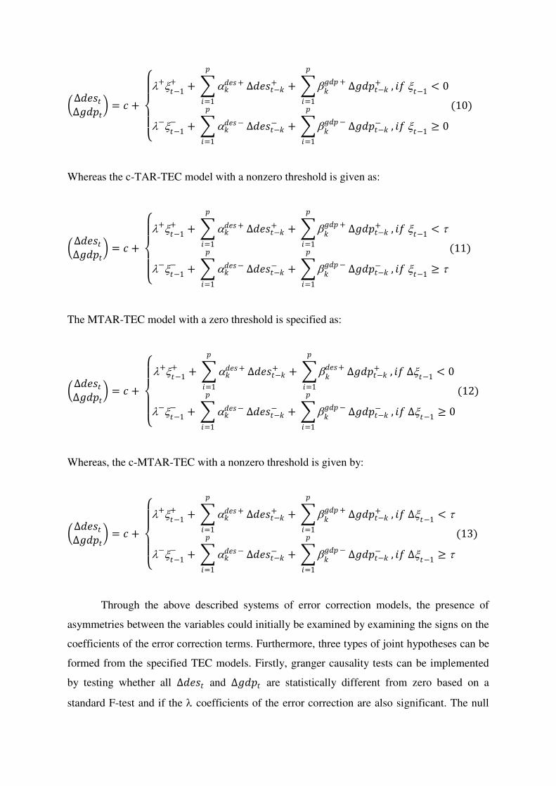
The MTAR-TEC model with a zero threshold is specified as:

∆𝑑𝑒𝑠𝑡∆𝑔𝑑𝑝𝑡 = 𝑐 +

+𝑡−1

++ 𝑘𝑑𝑒𝑠+ ∆𝑑𝑒𝑠𝑡−𝑘+

𝑝𝑖=1

+ 𝑘𝑑𝑒𝑠+ ∆𝑔𝑑𝑝𝑡−𝑘+

𝑝𝑖=1

, 𝑖𝑓 ∆𝑡−1< 0

−𝑡−1

−+ 𝑘𝑑𝑒𝑠− ∆𝑑𝑒𝑠𝑡−𝑘−𝑝

𝑖=1

+ 𝑘𝑔𝑑𝑝− ∆𝑔𝑑𝑝𝑡−𝑘−𝑝𝑖=1

, 𝑖𝑓 ∆𝑡−1≥ 0

(12)

Whereas, the c-MTAR-TEC with a nonzero threshold is given by:

∆𝑑𝑒𝑠𝑡∆𝑔𝑑𝑝𝑡 = 𝑐 +

+𝑡−1

++ 𝑘𝑑𝑒𝑠+ ∆𝑑𝑒𝑠𝑡−𝑘+

𝑝𝑖=1

+ 𝑘𝑔𝑑𝑝 + ∆𝑔𝑑𝑝𝑡−𝑘+

𝑝𝑖=1

, 𝑖𝑓 ∆𝑡−1<

−𝑡−1

−+ 𝑘𝑑𝑒𝑠− ∆𝑑𝑒𝑠𝑡−𝑘−𝑝

𝑖=1

+ 𝑘𝑔𝑑𝑝− ∆𝑔𝑑𝑝𝑡−𝑘−𝑝𝑖=1

, 𝑖𝑓 ∆𝑡−1≥

(13)

Through the above described systems of error correction models, the presence of

asymmetries between the variables could initially be examined by examining the signs on the

coefficients of the error correction terms. Furthermore, three types of joint hypotheses can be

formed from the specified TEC models. Firstly, granger causality tests can be implemented

by testing whether all ∆𝑑𝑒𝑠𝑡 and ∆𝑔𝑑𝑝𝑡 are statistically different from zero based on a

standard F-test and if the coefficients of the error correction are also significant. The null

hypothesis that ∆𝑑𝑒𝑠𝑡 dose not lead to ∆𝑔𝑑𝑝𝑡 can be denoted as: H03: k = 0, i=1, ...., k and

the null hypothesis that ∆𝑔𝑑𝑝𝑡 does not lead to ∆𝑑𝑒𝑠𝑡 is: H04: k = 0, i=1, ..., k. The second

type of hypothesis would be the cumulative symmetric effects which is relatively a long-run

test for asymmetry. The final hypothesis tests whether it is possible to get back to equilibrium

after a shock, and if it is the case, how long will it take. Since the causality tests are sensitive

to the selection of the lag length, we determine the lag lengths using the AIC criterion.

4. EMPIRICAL ANALYSIS

4.1 UNIVARIATE TIME SERIES ANALYSIS

Considering the nature of our research, the data used in the empirical analysis consists

of the annual percentage change in gross domestic product (GDP) which is gathered from the

South African Reserve Bank (SARB) website whereas nutrition is measured by calorie intake

expressed in calories/capita/day was collected from various food balance sheets (FAO, 2010).

The empirical analysis uses annually adjusted data obtained for the periods extending from

1960 to 2009. Our choice of sample period and periodicity reflects the limitations in the

availability of the time-series data on nutrition and economic growth for South Africa. We

also take into consideration the discussions of Hodge (2009) concerning the volatility

complexities associated with South African data and advocate on the use of filtering

techniques in order to smooth the data In particular, we apply the Hodrick-Prescott (HP) filter

to the time series variables prior to being incorporated into the econometric analysis.

Prior to testing for unit roots within the individual time series, we begin our analysis

by estimating self-exciting threshold autoregressive (SETAR) processes for the time series

variables as means of evaluating whether nonlinear behaviour exists amoung the observed

variables. In particular, we apply Hansen‟s (2000) conditional least squares (CLS) technique

which entails performing a grid-search over a predetermined range of threshold variable

estimates belonging to a set 𝛹 = [𝛾,𝛾, ] with the optimal estimates 𝛾 chosen by minimizing

the following objective functions 𝛾 = argmin𝛾𝜖𝛹 𝑄𝑇(𝛾). Once we obtain an estimate of 𝛾 ,

which maximizes the explanatory power of the SETAR regressions, the corresponding slope

coefficients and residual errors of the SETAR regressions are estimated via backward

substitution. As a means of validating the threshold effects, Hansen (2000) suggests the use

of a likelihood ratio (𝐿𝑅 𝜆 ) statistic which tests the null hypothesis of no threshold effects

against the alternative of threshold effects. In our empirical analysis, we obtain the following

estimates of the SETAR process for ∆𝑑𝑒𝑠𝑡: 𝑑𝑒𝑠𝑡 = 1.08 0.08 ∗𝑑𝑒𝑠𝑡−1 𝐼. 𝑑𝑒𝑠 ≤ 𝜆𝑑𝑒𝑠 + 0.36 0.07 ∗𝑑𝑒𝑠𝑡−1 𝐼. 𝑑𝑒𝑠 > 𝜆𝑑𝑒𝑠 (14) 𝜆𝑑𝑒𝑠 = 0.47; 𝐿𝑅(𝜆𝑑𝑒𝑠 ) = 12.42

(0.00)∗∗∗; 𝑅2 = 0.78; 𝐴𝐼𝐶 = −349; 𝑀𝐴𝑃𝐸 = 48.7%

Whereas for ∆𝑔𝑑𝑝 we estimate the following asymmetric data generating process:

𝑔𝑑𝑝𝑡 = 0.59 0.01 ∗∗𝑔𝑑𝑝𝑡−1 𝐼. 𝑔𝑑𝑝 ≤ 𝜆𝑔𝑑𝑝 + 1.64 0.02 ∗𝑑𝑒𝑠𝑡−1 𝐼. 𝑔𝑑𝑝 > 𝜆𝑔𝑑𝑝 (15) 𝜆𝑔𝑑𝑝 = 4.7; 𝐿𝑅(𝜆𝑔𝑑𝑝 ) = 10.67(0.00)∗∗∗; 𝑅2 = 0.76; 𝐴𝐼𝐶 = −214; 𝑀𝐴𝑃𝐸 = 3.205%

Our estimation results, as reported above, reveal that both 𝑑𝑒𝑠 and 𝑔𝑑𝑝 reject the null

hypothesis of no thresholds and are therefore rendered as SETAR (1,1) processes. Based

upon Hansen‟s (2000) SETAR modelling procedure, we obtain a threshold estimate of -

1.08% for 𝑑𝑒𝑠, whereas a threshold of 4.7% is estimated for 𝑔𝑑𝑝. In deciding the lag period

of the model, we apply the AIC and BIC rule to select the number of lag‟s to include and the

estimation results show that a lag of 1 period is optimal for the SETAR model. From the

coefficients of the lagged values in both the upper and lower regime, we find that 𝑑𝑒𝑠

behaves in a persistent manner and seems to contain a unit root above its threshold level,

whereas below this level 𝑑𝑒𝑠 is not persistent and seems to be stationary. Conversely,𝑔𝑑𝑝

tends to evolve as a stationary, non-persistent process above its threshold level and exhibits

unit root behaviour at rates of above 4.7 percent.

Distinguishing between nonlinearity and unit roots in the time series variables is

considered important since they render different dynamics over the business cycle. Unit roots,

on one hand, imply that a shock to either unemployment or output growth would lead to a

new natural rate in the long-run. On the other side of the spectrum, asymmetric behaviour in

the individual time series may be a result of hysteresis within the data generating process of

the time series. Enders and Granger (1998) and Enders and Siklos (2001) demonstrate the

problem of low power associated with traditional unit root tests when the underlying data

generating process of time series is found to be asymmetric. Therefore, in order to formally

validate our preliminary evidence of persistence amoung the variables, we proceed to apply

the nonlinear unit root test of Bec, Salem and Carrasco (2004) (BBC hereafter) in order to

test for the presence of unit roots against the null hypothesis of a stationary nonlinear SETAR

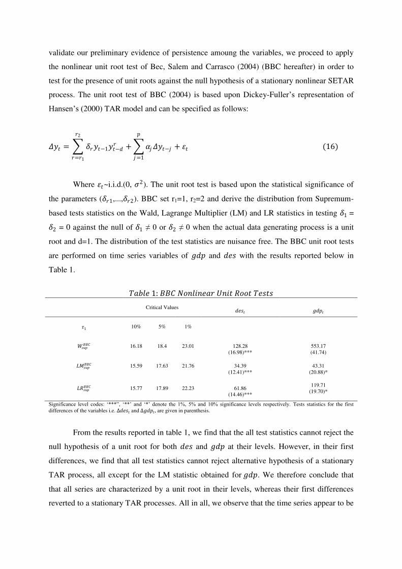
process. The unit root test of BBC (2004) is based upon Dickey-Fuller‟s representation of

Hansen‟s (2000) TAR model and can be specified as follows:

𝛥𝑦𝑡 = 𝛿𝑟𝑦𝑡−1𝑦𝑡−𝑑𝑟𝑟2

𝑟=𝑟1

+ 𝛼𝑗𝛥𝑦𝑡−𝑗𝑝𝑗=1

+ 𝜀𝑡 (16)

Where 𝜀𝑡~i.i.d.(0, 𝜎2). The unit root test is based upon the statistical significance of

the parameters (𝛿𝑟1,...,𝛿𝑟2). BBC set r1=1, r2=2 and derive the distribution from Supremum-

based tests statistics on the Wald, Lagrange Multiplier (LM) and LR statistics in testing 𝛿1 = 𝛿2 = 0 against the null of 𝛿1 ≠ 0 or 𝛿2 ≠ 0 when the actual data generating process is a unit

root and d=1. The distribution of the test statistics are nuisance free. The BBC unit root tests

are performed on time series variables of 𝑔𝑑𝑝 and 𝑑𝑒𝑠 with the results reported below in

Table 1.

𝑇𝑎𝑏𝑙𝑒 1: 𝐵𝐵𝐶 𝑁𝑜𝑛𝑙𝑖𝑛𝑒𝑎𝑟 𝑈𝑛𝑖𝑡 𝑅𝑜𝑜𝑡 𝑇𝑒𝑠𝑡𝑠

Critical Values

𝑑𝑒𝑠𝑡 𝑔𝑑𝑝𝑡 𝜏1

10% 5% 1%

𝑊𝑠𝑢𝑝𝐵𝐵𝐶

16.18 18.4 23.01

128.28

(16.98)***

553.17

(41.74)

𝐿𝑀𝑠𝑢𝑝𝐵𝐵𝐶

15.59 17.63 21.76

34.39

(12.41)***

43.31

(20.88)*

𝐿𝑅𝑠𝑢𝑝𝐵𝐵𝐶

15.77 17.89 22.23

61.86

(14.46)***

119.71

(19.70)*

Significance level codes: „***”, „**‟ and „*‟ denote the 1%, 5% and 10% significance levels respectively. Tests statistics for the first

differences of the variables i.e. Δ𝑑𝑒𝑠𝑡 and Δ𝑔𝑑𝑝𝑡 , are given in parenthesis.

From the results reported in table 1, we find that the all test statistics cannot reject the

null hypothesis of a unit root for both 𝑑𝑒𝑠 and 𝑔𝑑𝑝 at their levels. However, in their first

differences, we find that all test statistics cannot reject alternative hypothesis of a stationary

TAR process, all except for the LM statistic obtained for 𝑔𝑑𝑝. We therefore conclude that

that all series are characterized by a unit root in their levels, whereas their first differences

reverted to a stationary TAR processes. All in all, we observe that the time series appear to be

both nonlinear and non-stationary and as a result, we may (as a pre-speculation), assume that

the time-series variables tends to asymmetrically move more or less together over time, a

phenomenon that is later confirmed via formal co-integration analysis.

4.2 THRESHOLD COINTEGRATION MODEL ESTIMATES

Given evidence of all series being integrated of order I(1), we then proceed to test for

long-run equilibrium by employing the Ender and Silkos (2001) asymmetric cointegration

methodology. Table 2 below presents the results of the threshold cointegration analysis

performed for the nutrition and economic growth employing the TAR, c-TAR, MTAR and c-

MTAR model specifications.

𝑇𝑎𝑏𝑙𝑒 2: 𝑇𝑕𝑟𝑒𝑠𝑕𝑜𝑙𝑑 𝐶𝑜𝑖𝑛𝑡𝑒𝑔𝑟𝑎𝑡𝑖𝑜𝑛 𝑅𝑒𝑔𝑟𝑒𝑠𝑠𝑖𝑜𝑛𝑠 𝑑𝑒𝑝𝑒𝑛𝑑𝑒𝑛𝑡 𝑣𝑎𝑟𝑖𝑎𝑏𝑙𝑒

𝑑𝑒𝑠𝑡 𝑔𝑑𝑝𝑡 𝑚𝑜𝑑𝑒𝑙 𝑡𝑦𝑝𝑒

𝑡𝑎𝑟 𝑐 − 𝑡𝑎𝑟 𝑚𝑡𝑎𝑟 𝑐 −𝑚𝑡𝑎𝑟 𝑡𝑎𝑟 𝑐 − 𝑡𝑎𝑟 𝑚𝑡𝑎𝑟 𝑐 − 𝑚𝑡𝑎𝑟

𝜓𝑖0

-0.21

(0.00)***

-0.21

(0.00)***

-0.21

(0.00)***

-0.21

(0.00)***

1.84

(0.00)***

1.84

(0.00)***

1.84

(0.00)***

1.84

(0.00)*** 𝜓𝑖1

0.15

(0.00)***

0.15

(0.00)***

0.15

(0.00)***

0.15

(0.00)***

5.25

(0.00)***

5.25

(0.00)***

5.25

(0.00)***

5.25

(0.00)***

𝑡𝑕𝑟𝑒𝑠𝑕𝑜𝑙𝑑 𝑣𝑎𝑟𝑖𝑎𝑏𝑒/𝑣𝑎𝑙𝑢𝑒(𝜏)

0

0.038

0

0.015

0

0.07

0

-0.074

𝜌1𝜉𝑡−1

0.009

(0.00)***

0.009

(0.00)***

-0.011

(0.00)***

-0.02

(0.00)***

0.007

(0.00)***

-0.007

(0.00)***

-0.003

(0.103)*

-0.007

(0.00)***

𝜌2𝜉𝑡−1

-0.013

(0.00)***

-0.013

(0.00)***

0.009

(0.00)***

-0.01

(0.00)***

-0.008

(0.00)***

-0.008

(0.00)***

-0.011

(0.00)***

-0.004

(0.506)

𝛽𝐼𝛥𝜉𝑡−1

1.00

(0.00)***

1.00

(0.00)***

1.00

(0.00)***

1.02

(0.00)***

1.00

(0.00)***

1.00

(0.00)***

1.01

(0.00)***

0.99

(0.00)***

𝑅2

0.9895

0.9896

0.9899

0.9904

0.9851

0.9851

0.9873

0.9852

𝐻0:𝜌1 = 𝜌2 = 0

22.31

(0.00)***

22.51

(0.00)***

20.80

(0.00)***

23.19

(0.00)***

12.585

(0.00)***

12.57

(0.00)***

18.495

(0.00)***

12.699

(0.00)***

𝐻0:𝜌1 = 𝜌2

1.95

(0.169)

2.16

(0.148)

0.39

(0.535)

2.87

(0.098)*

0.21

(0.65)

0.19

(0.67)

7.76

(0.008)

0.35

(0.56)

𝑎𝑖𝑐

-495.72

-495.94

-494.10

-496.65

-336.414

-336.393

-343.828

-336.569

𝑏𝑖𝑐

-488.32

-488.54

-486.70

-489.25

-328.014

-328.992

-336.428

-329.168

𝑛𝑢𝑚𝑏𝑒𝑟 𝑜𝑓 𝑜𝑏𝑠𝑒𝑟𝑣𝑎𝑡𝑖𝑜𝑛𝑠

49

49

49

49

49

49

49

49

Asterisk (*) denotes 10% significance levels. Tests statistics for the coefficients from the threshold cointegration model and the p-values for

the hypothesis testing are all given in parenthesis.

The estimation results depict that there is indeed a long-run relationship between the

two variables as the null hypothesis of no cointegration is rejected in favour of the alternative

hypothesis of threshold cointegration for all the estimated models. This implies that the long-

run regression estimates can be interpreted with non-spurious interpretations. We find that for

the 𝑔𝑑𝑝 model regression, a one percent increase in the rate of nutrition intake is associated

with an increase in 𝑔𝑑𝑝 of roughly 5.2 percent. In terms of the nutrition-based efficiency

wage hypothesis, this result indicates that an improvement in nutritional intake will lead to an

improvement in productivity output, in terms of improved human capital input. Similar

interpretations are deduced from the 𝑑𝑒𝑠 regression, in which we find that a percentage

increase in 𝑔𝑑𝑝 results in an increase of nutritional intake of roughly 0.15 percent which

indicates an income elasticity of nutrient of 0.15 for the observed data which is significantly

different from zero. In translating this obtained result to the nutrition-based Engel curve, this

implies that improved productivity will lead to improved nutritional status of the economy. In

this sense, the above-described evidence leads to support of both the efficiency wage

hypothesis and the Engel curve for South African data. Overall, our long-run regression

elasticity estimates are in coherence with those obtained other studies like Bouis and Haddad

(1992) for the Phillipines; Babatunde (2008) for Nigeria and Reutlinger and Selowsky (1976)

for other emerging economies. It is also worth noting that all regression results have a strong

explanatory power with a general coefficient of determination (𝑅2) of 0.98 being observed.

Furthermore, all regressions passed the diagnostic tests such as the Durbin Watson (DW) for

autocorrelation.

Subsequent to estimating our long-run regression, we model the TAR and MTAR

variations of the residuals obtained from the 𝑑𝑒𝑠 and 𝑔𝑑𝑝 regressions (1) and (2). Using the

conditional least squares (CLS) method as described in Hansen (1999), we obtain threshold

values of 0.038 and 0.015, for the c-TAR and c-MTAR model when 𝑑𝑒𝑠 is employed as a

dependent variable, respectively. On the other hand, when 𝑔𝑑𝑝 is used as the dependent

variable, the estimated thresholds for the c-TAR and c-MTAR models are 0.07 and -0.074,

respectively. As previously mentioned, a sufficient condition for validating asymmetric

cointegration amoung the time series variables is that the residuals (i.e. ɛ𝑡) from equation (3)

must be stationary i.e. 1,2 < 0 and (1-1)(1-2) < 1. From table 2, we observe that only the

c-MTAR model using 𝑑𝑒𝑠 as a dependent variable and the c-TAR, MTAR and c-MTAR

model for 𝑔𝑑𝑝 as a dependent variable satisfy this condition. In the aforementioned models

where the condition of stationary residuals is satisfied, we find that the speed of adjustment

towards equilibrium is faster in the case of a shock to ɛ𝑡 . We also find that the absolute

parameter 1 is higher compared to the estimated 2 coefficient, for all estimated models with

exception of the c-MTAR models for both 𝑑𝑒𝑠 and 𝑔𝑑𝑝 regressions.

In turning to more formal asymmetric cointegration tests, we find that all estimated

models cannot reject the null hypothesis of symmetric cointegration in favour of the

alternative of asymmetric cointegration effects, with exception for the c-MTAR model with 𝑑𝑒𝑠 as a dependent variable. Therefore, as is based upon the presented empirical evidence,

the c-MTAR specification is deemed to provide the most adequate description of asymmetric

behaviour between the time series variables in contrast to the estimated TAR models.

Following this evidence, an asymmetric co-integration relationship between nutrition and

economic growth is validated and thus warrants the estimation of corresponding error

correction mechanism (ECM) with long-run asymmetric equilibrium.

4.3 THRESHOLD ERROR CORRECTION MODEL ESTIMATES

Having provided evidence supporting asymmetric adjustment, an asymmetric error

correction model can be used to investigate the movement of the time-series variables

towards their long-run equilibrium relationship. Table 3 reports the estimates of threshold

error correction (TEC) model as given by equations (8) to (11). For each of the model

specifications, the lag length was selected using the AIC information criterion. Key statistics

are reported in table 3, including the null hypothesis of granger causality tests, cumulative

asymmetric tests as well as symmetric momentum equilibrium adjustment path. It should be

noted that the estimates of our threshold error correction models for the TAR, c-TAR, MTAR

and c-MTAR models of both 𝑑𝑒𝑠 and 𝑔𝑑𝑝 as dependent variables are presented in table 3

inorder to provide a comparison between the obtained results.

𝑇𝑎𝑏𝑙𝑒 3: (𝑀)𝑇𝐴𝑅 − 𝑇𝐸𝐶 𝑅𝐸𝑆𝑈𝐿𝑇𝑆 𝑑𝑒𝑝𝑒𝑛𝑑𝑒𝑛𝑡 𝑣𝑎𝑟𝑖𝑎𝑏𝑙𝑒

∆𝑑𝑒𝑠𝑡 ∆𝑔𝑑𝑝𝑡 𝑚𝑜𝑑𝑒𝑙 𝑡𝑦𝑝𝑒

𝑡𝑎𝑟− 𝑡𝑒𝑐

𝑚𝑡𝑎𝑟− 𝑡𝑒𝑐

𝑐 − 𝑡𝑎𝑟− 𝑡𝑒𝑐

𝑐 −𝑚𝑡𝑎𝑟− 𝑡𝑒𝑐

𝑡𝑎𝑟− 𝑡𝑒𝑐

𝑚𝑡𝑎𝑟− 𝑡𝑒𝑐

𝑐 − 𝑡𝑎𝑟− 𝑡𝑒𝑐

𝑐 −𝑚𝑡𝑎𝑟− 𝑡𝑒𝑐

−𝑡−1

−

-0.036

(0.00)***

-0.036

(0.00)***

-0.0361

(0.00)***

-0.0383

(0.00)***

-0.056

(0.00)***

-0.057

(0.00)***

-0.0603

(0.00)***

-0.065

(0.00)*** ∆𝑑𝑒𝑠𝑡−𝑘−

0.8191

(0.00)***

0.8102

(0.00)***

0.8250

(0.00)***

0.7771

(0.00)***

0.2697

(0.04)*

0.5236

(0.00)***

0.2269

(0.09)*

0.3656

(0.01)* ∆𝑔𝑑𝑝𝑡−𝑘−

-0.0051

(0.84)

0.072

(0.00)***

0.0683

(0.00)***

0.083

(0.00)***

1.0332

(0.00)***

0.9657

(0.00)***

1.0474

(0.00)***

0.9983

(0.00)***

+𝑡−1

+

-0.0363

(0.02)*

-0.037

(0.00)***

-0.0326

(0.03)*

-0.0272

(0.00)***

-0.1319

(0.00)***

-0.038

(0.02)*

-0.1512

(0.00)***

-0.061

(0.00)** ∆𝑑𝑒𝑠𝑡−𝑘+

0.9163

(0.00)***

0.9144

(0.00)***

0.9336

(0.00)***

0.8676

(0.00)***

0.3059

(0.08)*

0.6761

(0.00)***

0.2147

(0.20)

0.6224

(0.00)*** ∆𝑔𝑑𝑝𝑡−𝑘+

-0.0051

(0.84)

-0.003

(0.78) -0.0116

(0.653)

-0.0029

(0.78) 0.9414

(0.00)***

0.7869

(0.00)***

0.9753

(0.00)***

0.8229

(0.00)*** 𝑅2

0.9994 0.9994 0.9994 0.9994 0.9998 0.9999 0.9999 0.9998

𝑛𝑢𝑚𝑏𝑒𝑟 𝑜𝑓 𝑜𝑏𝑠𝑒𝑟𝑣𝑎𝑡𝑖𝑜𝑛𝑠

49 49 49 49 49 49 49 49

𝐷𝑊

0.741

(0.00)***

0.75

(0.00)***

0.745

(0.00)***

0.776

(0.00)***

0.582

(0.00)***

0.65

(0.00)***

0.580

(0.00)***

0.550

(0.00)*** 𝐻1 0.000

(0.985)

0.118

(0.73)

0.066

(0.798)

3.569

(0.07)*

4.30

(0.45)**

6.13

(0.01)**

8.167

(0.00)***

0.000

(0.986) 𝐻20

19.783

(0.00)***

29.361

(0.00)***

20.877

(0.00)***

30.965

(0.00)***

396.38

(0.00)***

426.01

(0.00)***

429.99

(0.00)***

473.625

(0.00)*** 𝐻21 114.276

(0.00)***

348.71

(0.00)***

114.864

(0.00)***

206.986

(0.00)***

2.189

(0.13)*

37.67

(0.00)***

1.54

(0.23)

20.526

(0.00)*** 𝐻30 15.028

(0.00)***

58.31

(0.00)***

18.56

(0.00)***

61.909

(0.00)***

3.892

(0.05)*

59.26

(0.00)***

2.879

(0.09)*

37.127

(0.00)*** 𝐻31

3.079

(0.087)*

7.76

(0.08)*

4.267

(0.045)**

8.148

(0.00)***

0.075

(0.79)

3.03

(0.09)*

0.010

(0.920)

9.536

(0.00)*** 𝐻40

15.028

(0.00)***

58.31

(0.00)***

18.56

(0.00)***

61.909

(0.00)***

3.89

(0.06)*

59.26

(0.00)***

2.879

(0.09)*

37.127

(0.00)*** 𝐻41

3.079

(0.087)*

7.76

(0.08)*

4.267

(0.045)**

8.148

(0.00)***

0.075

(0.79)

3.03

(0.09)*

0.010

(0.920)

9.536

(0.00)***

Significance level codes: „***”, „**‟ and „*‟ denote the 1%, 5% and 10% significance levels respectively. P-values are reported in

parenthesis.

From the results presented in Table 3, the estimates of all error correction terms are

found to be significant for both the long-run and short-run regression estimates and the

predictive power of the asymmetric error-correction models as measured by the 𝑅2 statistic

are found to be encouragingly high. The sign and trend of deviations are important in

determining how quickly policymakers are likely to respond to deviations from equilibrium.

In particular, the value of the adjustment parameters determines the speed of reversion back

to steady-state equilibrium when nutrition and economic growth temporarily depart from

their underlying equilibrium relationship following either a negative or positive shock to the

variables. For instance, the p-values for the estimates of −𝑡−1

− and +𝑡−1

+ indicate that for

all econometric models, with the exception of the c-MTAR-TEC model, a positive shock to 𝑑𝑒𝑠 results in a quicker adjustment back to its long-run equilibrium in comparison to the

effect of a negative shock. Conversely, we find that for both TAR-TEC and C-TAR-TEC

models, a positive shock to 𝑔𝑑𝑝 will result in a much quicker reversion back to steady-state

equilibrium in contrast to a negative shock, whereas on the other hand, the M-TAR-TEC

model responds slightly stronger to negative shocks when compared to positive shocks. In

further taking into consideration the asymmetric cointegration tests on the TEC models, we

find that the F-statistic rejects that the null hypothesis of symmetric cointegration adjustment

(i.e. the coefficients − and +

are equal) for the TAR-TEC, MTAR-TEC and c-TAR-TEC

models on the ∆𝑔𝑑𝑝 regression whereas the same hypothesis can only be rejected for the c-

TAR-TEC model on the ∆𝑑𝑒𝑠 regression. Moreover, it should be noted that the adjustment

coefficients between the various models, and, do not appear noticeably different.

Moreover, we applied the Granger causality tests based on the TEC models to

examine causal relations between nutrition and economic growth. The hypotheses of granger

causality between nutrition and economic growth are assessed with F-tests. Generally

speaking, causality between the two time series variables is found to run bi-directional, with

the exception for the c-TAR-TEC model with ∆𝑔𝑑𝑝 as a dependent variable where causality

is found to run from 𝑔𝑑𝑝 to 𝑑𝑒𝑠. These results provide overwhelming evidence in favour of

nutritional-intake having a two-way co-relationship with wealth and income. This, in

conjunction with the significant estimates obtained from the cointegration results presented in

Table 2, strongly advocates for the existence of both the efficiency wage hypothesis and

Engel curve for the case of South Africa. However, nutrition appears to have a stronger

causal effect on 𝑔𝑑𝑝 compared to the impact of economic growth on nutritional intake, a

finding which is similar to that obtained in Tiffin and Dawson (2002) yet contrary to that

obtained in Wang and Taniguchi (2001). The threshold co-integration tests reveal significant

asymmetric co-integration for the c-MTAR-TEC with ∆𝑑𝑒𝑠 as a dependent variable and for

the TAR, M-TAR and c-TAR models with ∆𝑔𝑑𝑝 as a dependent variable. The p-values

obtained from the hypothesis testing short-run dynamics are found to be significant for all

model specifications with the exception of the TAR-TEC and MTAR-TEC models with

∆𝑔𝑑𝑝 as a dependent variable, in which only the short-run dynamics of the coefficients

associated with nutrition are found to be significant. Furthermore, the cumulative asymmetric

effects are also examined. We find strong evidence of asymmetric cumulative effects both

upwards and downwards for all estimated models. The final type of asymmetry examined is

the momentum equilibrium adjustment path asymmetries, in which all estimated models, with

the exception of the TAR models on the ∆𝑔𝑑𝑝 regression.

Several interesting facts emerge regarding the overall estimation of our asymmetric

cointegration and error correction model. In general, the results of the asymmetric co-

integration test for the TEC models as reported in table 3 are similar to those performed for

the co-integration models in table 2, in the sense of the c-MTAR model with ∆𝑑𝑒𝑠 as a

dependent variable, being the only regression which cannot reject alternative hypothesis of

asymmetric co-integration among the time series variables. Therefore our results indicate that

the 𝑑𝑒𝑠 (and not 𝑔𝑑𝑝) is responsible for asymmetric cointegration adjustments between the

two variables. In contrasting the four estimated models, the MTAR with consistent threshold

estimate is clearly the best model based upon the cointegration tests. According to the

presented empirical evidence, MTAR model has a better explanatory ability of asymmetric

cointegration between nutrition and economic growth in South Africa in comparison to their

counterpart TAR specifications. We, therefore, conclude our empirical analysis by declaring

that a smooth adjustment co-integration relation exists between nutritional intake and

economic growth in South Africa.

5. CONCLUSION OF THE STUDY

The United Nations Millennium Development Goals (MDG) deem that income

poverty and malnutrition, as indicators of poverty, should be halved by the year 2015 whereas

the Accelerated and Shared Growth of South Africa (ASGISA) have a set an economic

growth target of 6 percent as planned to be achieved by 2014. By analysing the asymmetric

cointegration effects between nutrition and economic growth for annual South African data,

our study presents a number of intriguing policy implications. In particular, we find strong

empirical evidence in support of both the efficiency wage hypothesis and the Engel curve for

South African data. We take this finding to be of considerable importance since it draws the

implication that the health status of the South African economy, through its nutritional intake,

bears a two-way relationship with productivity and ultimately income wealth. While the

common yet sole use of the income-elasticity of calorie intake, as obtained from the Engel

curve, may reveal how nutritional intake is affected income, it infers little to policymakers on

how productivity output affects the diet consumption within the economy. This result may

produce limitations on the efficiency of policy formulation, as it places policymakers under

the impression that the sole reliance on development strategies through nutritional programs

aimed at improving economic growth may be sufficient for overall economic development.

Our study therefore adheres that whatever the implied individual merits of

implemented developments policies are, they are consequentially of limited value if

policymakers do not directly address nutritional issues within economic development

programs. With specific reference to policymakers in developing or emerging economies and

for international aid agencies, an important conclusion which can be drawn from our study is

that all policies- including food aid – which enhance food security and reduce

undernourishment in developing countries can account for improvements in economic

growth. In advocating for improved policies which strengthen food security by focusing on

their humanitarian benefits, the implications drawn from our study may serve as a reminder

that the direct focus on nutrition policies should neither be ignored or be planned in isolation

but should be implemented in conjunction with economic growth policies. On the other end

of the spectrum, relying solely upon labour markets interventions and economic growth

strategies is not sufficient enough to eradicate current poverty problems. We conclude that

the economic returns to investing in nutritional programs far outweigh their costs and policy

reforms supporting productivity growth need to be accompanied by strategic investment

programs aimed at tackling the overriding problem of poverty via nutrition- specific

development programs.

While we are able to establish a significant, positive correlation between nutrition and

economic growth we, however, interpret our overall findings with extreme caution as the

asymmetries found in the cointegration relation between nutritional intake and economic

growth in South Africa present reservations with regards to interpreting our obtained

empirical results. Specifically, we find that the cointegration asymmetries in the nutrition-

productivity co-relation are a result of slow adjustments back to the long-run steady-state

equilibrium in the face of negative and positive shocks to both nutrition and productivity

output. In other words, policy-induced shocks to either nutritional intake or productivity

output, as implemented through various development policies, will result in slow reversion or

responses to the counter variable as they deviate from cointegrated long-run steady state

equilibrium. A plausible explanation for such a long delay in the equilibrium adjustment

process following a shock to the variables, may be that policymakers have not yet identified

and thus explored other possible “avenues” which directly link nutritional programs towards

improved economic growth and vice-versa. Identifying and exploring the use these

intermediary channels between nutrition intake and economic growth may serve well as a

candidate for potential future research.

REFERENCES

Arcand J. (2001), “Undernourishment and economic growth: The efficacy cost of hunger”,

FAO Economic and Social Development Paper, 147, Rome, Italy.

Arora V. and Vamvakidis A. (2005), “The implications of South African growth for the rest

of Africa”, IMF Working Papers No. 05-58, March.

Blake N. and Fombly T. (1997), “Threshold co-integration”, International Economic Review,

38, 627-645.

Babatunde R. (2008), “Empirical analysis of the impact of income on dietary calorie intake in

Nigeria, European Journal of Social Sciences, 5(4), 174-181.

Bec F., Salem M. and Carrasco M. (2004), “Tests for unit root versus threshold specification

with an application to purchasing power parity relationship”, Journal of Business and

Economic Statistics, 22, 382-395.

Beechey M. and Osterholm P. (2008), “Revisiting the uncertain unit root in GDP and CPI:

testing for nonlinear trend reversion”, Economic Letters, 100, 221-223.

Behrman J. and Deolalikar A. (1987), “Will developing country nutrition improve with

income? A case study for rural South India”, Journal of Political economy, 95(3), 492-507.

Behrman J. and Deolalikar A. (1989), “Is variety the spice of life? Implications for calorie

intake”, The Review of Economics and Statistics, 71(4), 666-672.

Bouis H. and Haddad L. (1992), “Are estimates of calorie-income elasticities too high?”,

Journal of Development Economics, 39, 333-364.

Crespo-Cuaresma J. (2000), “Forecasting European GDP using a self-exciting threshold

autoregressive models. A warning”, Economic Series 79, Institute for Advanced Studies,

March.

Cole W. (1971), “Investment in nutrition as a factor of economic growth of developing

countries”, Land Economics, 47, 139-149.

Correa and Cummins (1970), “Contribution of nutrition to economic growth”, The American

Journal of Clinical Nutrition, 23(5), 560-565.

Deolalikar A. (1988), “Nutrition and labour productivity in agriculture: Estimates for rural

South India”, The Review of Economics and Statistics, 70(3), 406-413.

Enders and Dibooglu (2001), “Long-run purchasing power parity with asymmetric

adjustment”, Southern Economic Journal, 68(2), 433-445.

Enders W. and Silkos P. (2001), “Cointegration and threshold adjustment”, Journal of

Business and Economic Statistics, 19, 166-176.

Engle R. and Granger C. (1987), “Co-integration and error correction: Representation,

estimation and testing”, Econometrica, 55(2), 251-276.

Fan S. and Pandya-Lorch R. (2011), “Reshaping agriculture for nutrition and health”,

International Food Policy Research Institute, Washington, D.C.

Fogel R. (2004), “Health, nutrition and economic growth”, Economic Development and

Cultural Change, 52(3), 643-658.

Granger C. (1969), “Investigating causal relations by econometric models and cross-spectral

methods”, Econometrica, 37(3), 424-438.

Halicioglu F. (2011), “The demand for calories in Turkey”, MPRA Paper No. 41807,

October.

Hansen B. (2000), “Sample splitting and threshold estimation”, Econometrica, 68(3), 575-

604.

Heltberg (2009), “Malnutrition, poverty and economic growth”, Health Economics, 18. 77-

88.

Johansen S. (1991), “Estimation and hypothesis testing of co-integration vectors in gaussain

vector autoregressive models, Econometrica, 59, 1551-1580.

Khamfula Y. (2005), “Macroeconomic policies, shocks and economic growth in South

Africa”, Paper presented at the Macroeconomic Policy Challenges in Low Income Countries

Conference, IMF Headquarters, Washington: DC.

Leibenstein H. (1957), “The theory of underemployment in backward economies”, Journal of

Political Economy, 65(2), 91-103.

Meng X., Gong X. and Wang Y. (2004), “Impact of income growth and economic reform on

nutrition intake in urban China”, IZA Discussion Papers No. 1448, December.

Mirrlees J. (1976), “A pure theory of underdevelopment economies”, In L.G. Reynolds (ed)

Agriculture in Development Theory, Yale University Press: New Haven CT.

Mondal B, Chattopadhyay M. And Gupta R. (2005), “Economic condition and nutritional

status: A micor level study amoung tribal population in rural West Bengal, India”, Malaysian

Journal of Nutrition, 11(2), 99-109.

Ogundari K. (2011),” Estimating demand for nutrients in Nigeria: A vector error correction

model”, MPRA Paper No. 28930, February.

Ogundari K. And Abdulai A. (2013), “Examining the heterogeneity in calorie-income

elasticity: A meta-analysis”, Food Policy, 40, 119-128.

Neeliah H. and Shankar B. (2008), “Is nutritional improvement a cause or a consequence of

economic growth? Evidence from Mauritius”, Economics Bulletin, 17(8), 1-11.

Reutlinger S. and Selowsky M. (1976), “Malnutrition and poverty”, World Bank Staff

Occasional Papers No. 23, John Hopkins, Baltimore and London.

Salois M., Tiffin R. and Balcombe K. (2010), “Calorie and nutrient consumption as a

function of income: A cross country”, MPRA Paper No. 24726, August.

Shelly G. and Wallace F. (2011), “Further evidence regarding nonlinear trend reversion of

real GDP and the CPI”, Economic Letters, 112(1), 56-59.

Shimokawa S. (2010), “Asymmetric intra-household allocation of calories in China”,

American Journal of Agricultural Economics, 92(3), 873-888.

Skoufias E., Di Maro V., Gonzalez-Cossio T. and Ramirez S. (2009), “Nutrient consumption

and household income in rural Mexico”, Agriculture Economics, 40, 657-675.

Strauss J. (1986), “Does better nutrition raise farm productivity”, Journal of Political

Economy, 94(2), 297-320.

Strauss J. and Thomas D. (1997), “Health and wages: Evidence on men and women in urban

Brazil”, Journal of Econometrics, 77(1), 159-185.

Strauss J. and Thomas D. (1998), “Health, nutrition and economic growth”, Journal of

Economic Literature, 36(2), 766-817.

Stiglitz J. (1976), “The efficiency wage hypothesis, surplus labour and the distribution of

income in LDC‟s”, Oxford Economic Papers, 28, 185-207.

Svedberg P. (1999), “841 million undernourished”, World Development, 27, 2081-2098.

Taniguchi K. and Wang X. (2003), “Nutrition intake ad economic growth: Studies on the cost

of hunger, Food and Agriculture Organization of the United States, Rome, Italy.

Thomas D. and Frankenberg E. (2002), “Health, nutrition and prosperity”, Bulletin of the

World Health Organization, 80, 106-113.

Tiffin R. and Dawson P. (2002), “The demand for calories: Some further estimates from

Zimbabwe, Journal of Agriculture Economics, 53(2), 221-232.

Vecchi G. and Coppola M. (2003), “Nutrition and economic growth in Italy, 1861-1911.

What macroeconomic data hide”, Explorations in Economic History, 43(3), 438-464.