Astrophys. J. in press

Numerical Study on GRB-Jet Formation in Collapsars

Shigehiro Nagataki1,2, Rohta Takahashi3, Akira Mizuta4, Tomoya Takiwaki5

ABSTRACT

Two-dimensional magnetohydrodynamic simulations are performed using the

ZEUS-2D code to investigate the dynamics of a collapsar that generates a GRB

jet, taking account of realistic equation of state, neutrino cooling and heating

processes, magnetic fields, and gravitational force from the central black hole

and self gravity. It is found that neutrino heating processes are not so efficient

to launch a jet in this study. It is also found that a jet is launched mainly by

Bφ fields that are amplified by the winding-up effect. However, since the ratio of

total energy relative to the rest mass energy in the jet is not so high as several

hundred, we conclude that the jets seen in this study are not be a GRB jet. This

result suggests that general relativistic effects, which are not included in this

study, will be important to generate a GRB jet. Also, the accretion disk with

magnetic fields may still play an important role to launch a GRB jet, although

a simulation for much longer physical time (∼ 10 − 100 s) is required to confirm

this effect. It is shown that considerable amount of 56Ni is synthesized in the

accretion disk. Thus there will be a possibility for the accretion disk to supply

sufficient amount of 56Ni required to explain the luminosity of a hypernova. Also,

it is shown that neutron-rich matter due to electron captures with high entropy

per baryon is ejected along the polar axis. Moreover, it is found that the electron

fraction becomes larger than 0.5 around the polar axis near the black hole by

νe capture at the region. Thus there will be a possibility that r-process and

r/p−process nucleosynthesis occur at these regions. Finally, much neutrons will

1Yukawa Institute for Theoretical Physics, Kyoto University, Oiwake-cho Kitashirakawa Sakyo-ku, Kyoto

606-8502, Japan, E-mail: nagataki@yukawa.kyoto-u.ac.jp

2KIPAC, Stanford University, P.O.Box 20450, MS 29, Stanford, CA, 94309

3Graduate School of Arts and Sciences, The University of Tokyo, Tokyo 153-8902, Japan

4Max-Planck-Institute fur Astrophysik, Karl-Schwarzschild-Str. 1, 85741 Garching, Germany

5Department of Physics, The University of Tokyo, Bunkyo-ku, Tokyo 113-0033, Japan

– 2 –

be ejected from the jet, which suggests that signals from the neutron decays may

be observed as the delayed bump of the light curve of the afterglow or gamma-

rays.

Subject headings: gamma rays: bursts — accretion, accretion disks — black hole

physics — MHD — supernovae: general — nucleosynthesis

1. INTRODUCTION

There has been growing evidence linking long gamma-ray bursts (GRBs; in this study,

we consider only long GRBs, so we refer to long GRBs as GRBs hereafter for simplicity)

to the death of massive stars. The host galaxies of GRBs are star-forming galaxies and

the positions of GRBs appear to trace the blue light of young stars (Vreeswijk et al. 2001;

Bloom et al. 2002; Gorosabel et al. 2003). Also, ’bumps’ observed in some afterglows can be

naturally explained as contribution of bright supernovae (Bloom et al. 1999; Reichart 1999;

Galama et al. 2000; Garnavich et al. 2003). Moreover, direct evidence of some GRBs ac-

companied by supernovae have been reported such as the association of GRB 980425 with SN

1998bw (Galama et al. 1998; Iwamoto et al. 1998), that of GRB 030329 with SN 2003dh (Hjorth et al. 2003

Price et al. 2003; Stanek et al. 2003), and that of GRB 060218 and SN 2006aj (Mirabal et al. 2006;

Mazzali et al. 2006).

It should be noted that these supernovae (except for SN 2006aj) are categorized as a

new type of supernovae with large kinetic energy (∼ 1052 ergs), nickel mass (∼ 0.5M), and

luminosity (Iwamoto et al. 1998; Woosley et al. 1999), so these supernovae are sometimes

called hypernovae. The total explosion energy of the order of 1052 erg is too important to be

emphasized, because it is generally considered that a normal core-collapse supernova cannot

cause such an energetic explosion. Thus another scenario has to be considered to explain

the system of a GRB associated with a hypernova. One of the most promising scenarios is

the collapsar scenario (Woosley 1993). In the collapsar scenario, a black hole is formed as

a result of gravitational collapse. Also, rotation of the progenitor plays an essential role.

Due to the rotation, an accretion disk is formed around the equatorial plane. On the other

hand, the matter around the rotation axis freely falls into the black hole. MacFadyen and

Woosley (1999) pointed out that the jet-induced explosion along the rotation axis may occur

due to the heating through neutrino anti-neutrino pair annihilation that are emitted from

the accretion disk (see also Fryer and Meszaros 2000).

It is true that the collapsar scenario is the breakthrough on the problem of the cen-

tral engine of GRBs. However, there are many effects that have to be involved in order

– 3 –

to establish the scenario firmly. First of all, neutrino heating effects have to be investi-

gated carefully by including microphysics of neutrino processes in the numerical simula-

tions. It is true that MacFadyen and Woosley (1999) have done the numerical simulations

of the collapsar, in which a jet is launched along the rotation axis, but detailed micro-

physics of neutrino heating is not included in their simulations. Secondly, it was pointed

out that effects of magnetic fields and rotation may play an important role to launch

the GRB jets (Proga et al. 2003; Mizuno et al. 2004a; Mizuno et al. 2004b; Proga 2005;

Shibata and Sekiguchi 2005; Sekiguchi and Shibata 2005; Fujimoto et al. 2006), although

neutrino heating effects are not included in their works. Recently, Rockefeller et al (2006)

presented 3-dimensional simulations of collapsars with smoothed particle hydrodynamics

code. In their study, 3-flavor flux-limited diffusion package is used to take into account neu-

trino cooling and absorption of electron-type neutrinos, although neutrino anti-neutrino pair

annihilation is not included. They have shown that alpha-viscosity drives energetic explosion

through 3-dimensional instabilities and angular momentum transfer, although the jet is not

launched and magnetic fields (source of the viscosity) are not included in their study. Thus

it is not clear which effects are most important to launch a GRB jet, that is, what process

is essential as the central engine of GRBs.

Due to the motivation mentioned above, we have performed two-dimensional magne-

tohydrodynamic simulations of collapsars with magnetic fields, rotation, and neutrino cool-

ing/heating processes. In our simulations, the realistic equation of state (EOS) of Blinnikov

et al. (1996) and effects of photo-disintegration of nuclei are also included. We investigated

influence of magnetic fields on the dynamics of collapsars by changing initial amplitude of

the magnetic fields. In section 2, models and numerical methods are explained. Results are

shown in section 3. Discussions are described in 4. Summary and conclusion are presented

in section 5.

2. MODELS AND NUMERICAL METHODS

Our models and numerical methods of simulations in this study are shown in this section.

First we present equations of ideal MHD, then initial and boundary conditions are explained.

Micro physics included in this study (equation of state (EOS), nuclear reactions, and neutrino

processes) is also explained.

– 4 –

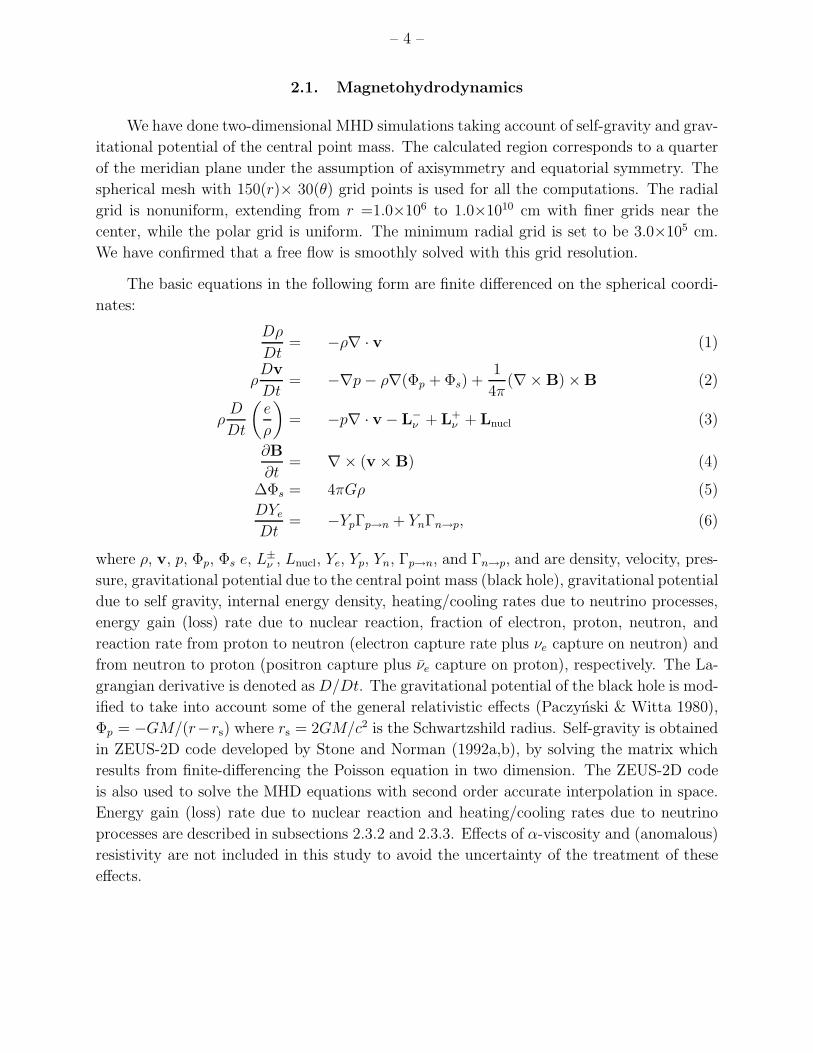
2.1. Magnetohydrodynamics

We have done two-dimensional MHD simulations taking account of self-gravity and grav-

itational potential of the central point mass. The calculated region corresponds to a quarter

of the meridian plane under the assumption of axisymmetry and equatorial symmetry. The

spherical mesh with 150(r)× 30(θ) grid points is used for all the computations. The radial

grid is nonuniform, extending from r =1.0×106 to 1.0×1010 cm with finer grids near the

center, while the polar grid is uniform. The minimum radial grid is set to be 3.0×105 cm.

We have confirmed that a free flow is smoothly solved with this grid resolution.

The basic equations in the following form are finite differenced on the spherical coordi-

nates:

Dρ

Dt= −ρ∇ · v (1)

ρDv

Dt= −∇p− ρ∇(Φp + Φs) +

1

4π(∇× B) ×B (2)

ρD

Dt

(

e

ρ

)

= −p∇ · v − L−ν + L+

ν + Lnucl (3)

∂B

∂t= ∇× (v × B) (4)

∆Φs = 4πGρ (5)

DYe

Dt= −YpΓp→n + YnΓn→p, (6)

where ρ, v, p, Φp, Φs e, L±ν , Lnucl, Ye, Yp, Yn, Γp→n, and Γn→p, and are density, velocity, pres-

sure, gravitational potential due to the central point mass (black hole), gravitational potential

due to self gravity, internal energy density, heating/cooling rates due to neutrino processes,

energy gain (loss) rate due to nuclear reaction, fraction of electron, proton, neutron, and

reaction rate from proton to neutron (electron capture rate plus νe capture on neutron) and

from neutron to proton (positron capture plus νe capture on proton), respectively. The La-

grangian derivative is denoted as D/Dt. The gravitational potential of the black hole is mod-

ified to take into account some of the general relativistic effects (Paczynski & Witta 1980),

Φp = −GM/(r−rs) where rs = 2GM/c2 is the Schwartzshild radius. Self-gravity is obtained

in ZEUS-2D code developed by Stone and Norman (1992a,b), by solving the matrix which

results from finite-differencing the Poisson equation in two dimension. The ZEUS-2D code

is also used to solve the MHD equations with second order accurate interpolation in space.

Energy gain (loss) rate due to nuclear reaction and heating/cooling rates due to neutrino

processes are described in subsections 2.3.2 and 2.3.3. Effects of α-viscosity and (anomalous)

resistivity are not included in this study to avoid the uncertainty of the treatment of these

effects.

– 5 –

2.2. Initial and Boundary Conditions

We adopt the model E25 in Heger et al. (2000). This model corresponds to a star that

has 25M initially with solar metallicity, but loses its mass and becomes to be 5.45M of a

Wolf-Rayet star at the final stage. This model seems to be a good candidate as a progenitor

of a GRB since losing their envelope will be suitable to be a Type Ic-like supernova and

to make a baryon poor fireball. The mass of the iron core is 1.69M in this model. Thus

we assume that the iron core has collapsed and formed a black hole at the center. This

treatment is same with Proga et al. (2003). The Schwartzshild radius of the black hole is

5.0×105 cm initially.

We explain how the angular momentum is distributed initially. At first, we performed

1-D simulation for the spherical collapse of the progenitor for 0.1 s when the inner most

Si-layer falls to the inner most boundary (=106 cm). After the spherical collapse, angular

momentum was distributed so as to provide a constant ratio of 0.05 of centrifugal force to the

component of gravitational force perpendicular to the rotation axis at all angles and radii,

except where that prescription resulted in j16 greater than a prescribed maximum value, 10.

This treatment is similar to the one in MacFadyen and Woosley (1999). The total initial

rotation energy is 2.44×1049 erg that corresponds to 1.3×10−2 for initial ratio of the rotation

energy to the gravitational energy (T/W ).

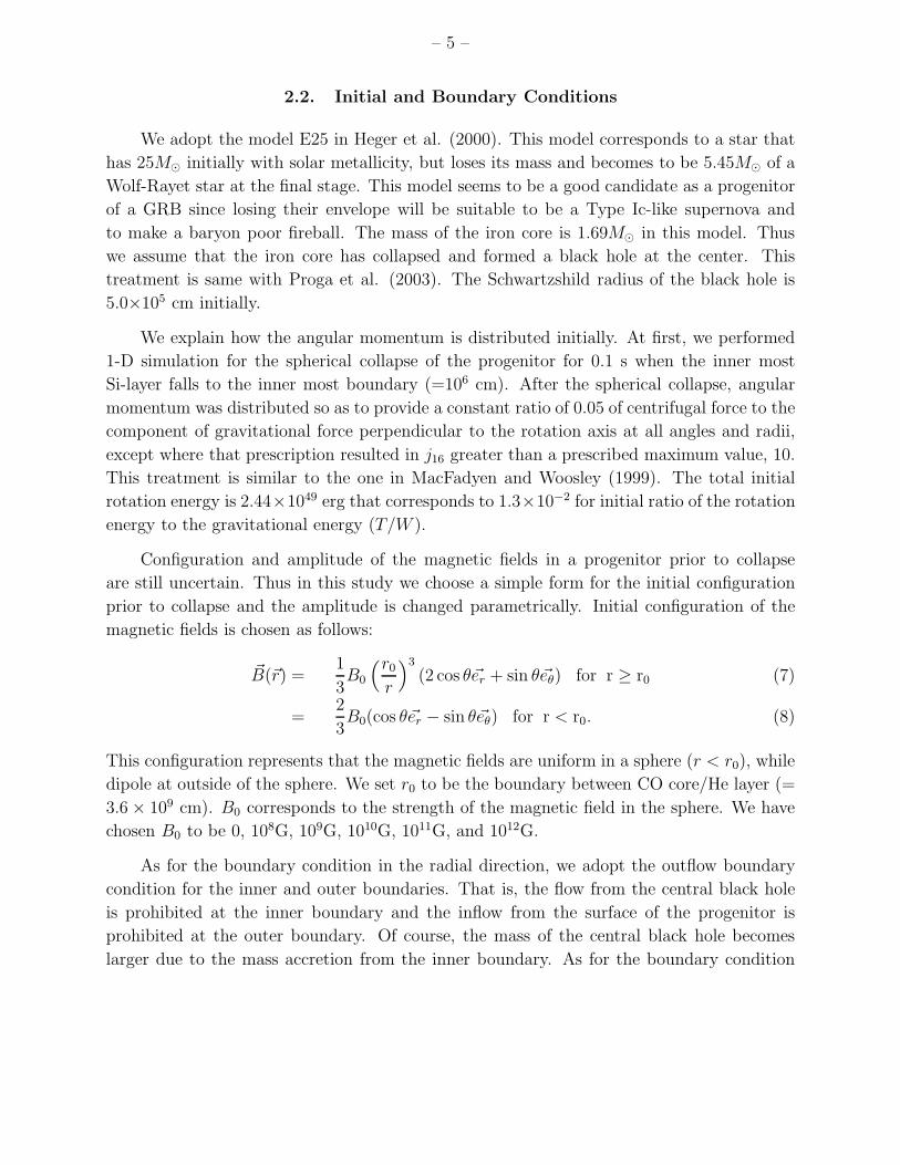
Configuration and amplitude of the magnetic fields in a progenitor prior to collapse

are still uncertain. Thus in this study we choose a simple form for the initial configuration

prior to collapse and the amplitude is changed parametrically. Initial configuration of the

magnetic fields is chosen as follows:

~B(~r) =1

3B0

(r0r

)3

(2 cos θ~er + sin θ~eθ) for r ≥ r0 (7)

=2

3B0(cos θ~er − sin θ~eθ) for r < r0. (8)

This configuration represents that the magnetic fields are uniform in a sphere (r < r0), while

dipole at outside of the sphere. We set r0 to be the boundary between CO core/He layer (=

3.6 × 109 cm). B0 corresponds to the strength of the magnetic field in the sphere. We have

chosen B0 to be 0, 108G, 109G, 1010G, 1011G, and 1012G.

As for the boundary condition in the radial direction, we adopt the outflow boundary

condition for the inner and outer boundaries. That is, the flow from the central black hole

is prohibited at the inner boundary and the inflow from the surface of the progenitor is

prohibited at the outer boundary. Of course, the mass of the central black hole becomes

larger due to the mass accretion from the inner boundary. As for the boundary condition

– 6 –

in the zenith angle direction, axis of symmetry boundary condition is adopted for the rota-

tion axis, while the reflecting boundary condition is adopted for the equatorial plane. As

for the magnetic fields, the equatorial symmetry boundary condition, in which the normal

component is continuous and the tangential component is reflected, is adopted.

2.3. Micro Physics

2.3.1. Equation of State

The equation of state (EOS) used in this study is the one developed by Blinnikov et

al. (1996). This EOS contains an electron-positron gas with arbitrary degeneracy, which is

in thermal equilibrium with blackbody radiation and ideal gas of nuclei. We used the mean

atomic weight of nuclei to estimate the ideal gas contribution to the total pressure, although

its contribution is negligible relative to those of electron-positron gas and thermal radiation

in our simulations.

2.3.2. Nuclear Reactions

Although the ideal gas contribution of nuclei to the total pressure is negligible, ef-

fects of energy gain/loss due to nuclear reactions are important. In this study, nuclear

statistical equilibrium (NSE) was assumed for the region where T ≥ 5 × 109 [K] is satis-

fied. This treatment is based on the assumption that the timescale to reach and maintain

NSE is much shorter than the hydrodynamical time. Note that complete Si-burning oc-

curs in explosive nucleosynthesis of core-collapse supernovae for the region T ≥ 5 × 109

[K] (Thielemann et al. 1996). The hydrodynamical time in this study, ∼ s (as shown in

Figs 3, 4, and 10, the nuclear reaction occurs at ∼ (107 − 108)cm where the radial velocity

is of the order of (107 − 108) cm s−1), is comparable to the explosive nucleosynthesis in core-

collapse supernovae, so the assumption of NSE adopted in this study seems to be well. 5

nuclei, n, p,4 He,16 O, and 56Ni were used to estimate the binding energy of ideal gas of nuclei

in NSE for given (ρ, T , Ye). Ye is electron fraction that is obtained from the calculations of

neutrino processes in section 2.3.3. On the other hand, we assumed that no nuclear reaction

occurs for the region where T < 5 × 109 [K].

– 7 –

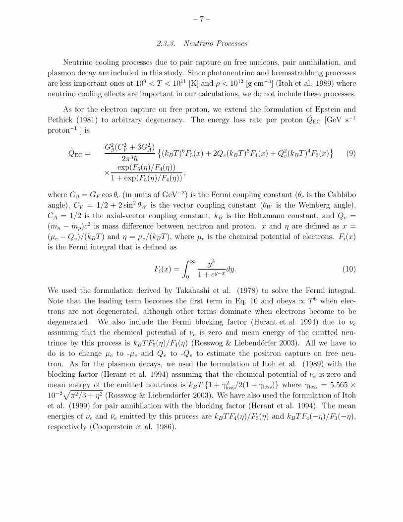
2.3.3. Neutrino Processes

Neutrino cooling processes due to pair capture on free nucleons, pair annihilation, and

plasmon decay are included in this study. Since photoneutrino and bremsstrahlung processes

are less important ones at 109 < T < 1011 [K] and ρ < 1012 [g cm−3] (Itoh et al. 1989) where

neutrino cooling effects are important in our calculations, we do not include these processes.

As for the electron capture on free proton, we extend the formulation of Epstein and

Pethick (1981) to arbitrary degeneracy. The energy loss rate per proton QEC [GeV s−1

proton−1 ] is

QEC =G2

β(C2V + 3G2

A)

2π3~

(kBT )6F5(x) + 2Qv(kBT )5F4(x) +Q2v(kBT )4F3(x)

(9)

× exp(F5(η)/F4(η))

1 + exp(F5(η)/F4(η)),

where Gβ = GF cos θc (in units of GeV−2) is the Fermi coupling constant (θc is the Cabbibo

angle), CV = 1/2 + 2 sin2 θW is the vector coupling constant (θW is the Weinberg angle),

CA = 1/2 is the axial-vector coupling constant, kB is the Boltzmann constant, and Qv =

(mn − mp)c2 is mass difference between neutron and proton. x and η are defined as x =

(µe − Qv)/(kBT ) and η = µe/(kBT ), where µe is the chemical potential of electrons. Fi(x)

is the Fermi integral that is defined as

Fi(x) =

∫

∞

0

yk

1 + ey−xdy. (10)

We used the formulation derived by Takahashi et al. (1978) to solve the Fermi integral.

Note that the leading term becomes the first term in Eq. 10 and obeys ∝ T 6 when elec-

trons are not degenerated, although other terms dominate when electrons become to be

degenerated. We also include the Fermi blocking factor (Herant et al. 1994) due to νe

assuming that the chemical potential of νe is zero and mean energy of the emitted neu-

trinos by this process is kBTF5(η)/F4(η) (Rosswog & Liebendorfer 2003). All we have to

do is to change µe to -µe and Qv to -Qv to estimate the positron capture on free neu-

tron. As for the plasmon decays, we used the formulation of Itoh et al. (1989) with the

blocking factor (Herant et al. 1994) assuming that the chemical potential of νe is zero and

mean energy of the emitted neutrinos is kBT 1 + γ2loss/2(1 + γloss) where γloss = 5.565 ×

10−2√

π2/3 + η2 (Rosswog & Liebendorfer 2003). We have also used the formulation of Itoh

et al. (1999) for pair annihilation with the blocking factor (Herant et al. 1994). The mean

energies of νe and νe emitted by this process are kBTF4(η)/F3(η) and kBTF4(−η)/F3(−η),respectively (Cooperstein et al. 1986).

– 8 –

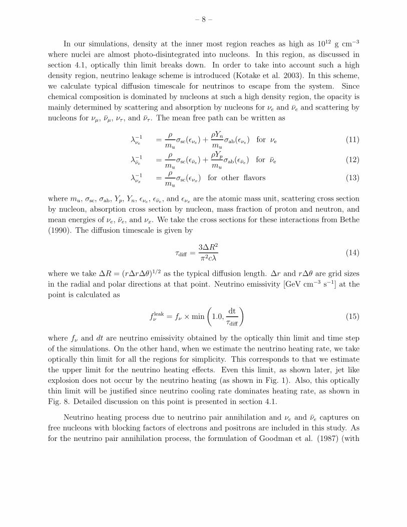
In our simulations, density at the inner most region reaches as high as 1012 g cm−3

where nuclei are almost photo-disintegrated into nucleons. In this region, as discussed in

section 4.1, optically thin limit breaks down. In order to take into account such a high

density region, neutrino leakage scheme is introduced (Kotake et al. 2003). In this scheme,

we calculate typical diffusion timescale for neutrinos to escape from the system. Since

chemical composition is dominated by nucleons at such a high density region, the opacity is

mainly determined by scattering and absorption by nucleons for νe and νe and scattering by

nucleons for νµ, νµ, ντ , and ντ . The mean free path can be written as

λ−1νe

=ρ

mu

σsc(ενe) +

ρYn

mu

σab(ενe) for νe (11)

λ−1νe

=ρ

mu

σsc(ενe) +

ρYp

mu

σab(ενe) for νe (12)

λ−1νx

=ρ

muσsc(ενx

) for other flavors (13)

where mu, σsc, σab, Yp, Yn, ενe, ενe

, and ενxare the atomic mass unit, scattering cross section

by nucleon, absorption cross section by nucleon, mass fraction of proton and neutron, and

mean energies of νe, νe, and νx. We take the cross sections for these interactions from Bethe

(1990). The diffusion timescale is given by

τdiff =3∆R2

π2cλ(14)

where we take ∆R = (r∆r∆θ)1/2 as the typical diffusion length. ∆r and r∆θ are grid sizes

in the radial and polar directions at that point. Neutrino emissivity [GeV cm−3 s−1] at the

point is calculated as

f leakν = fν × min

(

1.0,dt

τdiff

)

(15)

where fν and dt are neutrino emissivity obtained by the optically thin limit and time step

of the simulations. On the other hand, when we estimate the neutrino heating rate, we take

optically thin limit for all the regions for simplicity. This corresponds to that we estimate

the upper limit for the neutrino heating effects. Even this limit, as shown later, jet like

explosion does not occur by the neutrino heating (as shown in Fig. 1). Also, this optically

thin limit will be justified since neutrino cooling rate dominates heating rate, as shown in

Fig. 8. Detailed discussion on this point is presented in section 4.1.

Neutrino heating process due to neutrino pair annihilation and νe and νe captures on

free nucleons with blocking factors of electrons and positrons are included in this study. As

for the neutrino pair annihilation process, the formulation of Goodman et al. (1987) (with

– 9 –

blocking factors) is adopted. The νe and νe captures on free nucleons are inverse processes

of electron/positron captures. The calculation of neutrino heating is the most expensive in

the simulation of this study. Thus, to save the CPU time, the neutrino heating processes

are calculated only within the limited regions (r < 109 cm). Moreover, we adopt some

criterions as follows in order to save CPU time. We have to determine the energy deposition

regions and emission regions to estimate the neutrino heating rate. As for the neutrino pair

annihilation process, We adopt no criterion for the energy deposition regions other than

r < 109 cm, while the emission regions satisfy the criterion of T ≥ 3 × 109 K. As for the

neutrino capture process, we adopt the criterions as follows: The absorption regions should

satisfy the criterion of ρ ≥ 104 g cm−3, while the emission regions satisfy the criterion of (i)

ρ ≥ 103 g cm−3 and (ii) T ≥ 109 K. Also, these heating rate had to be updated every 100

time steps to save CPU time. Of course this treatment has to be improved in the future.

However, this treatment seems to be justified as follows: The total time step is of the order

of 106 steps. The final physical time is of the order of seconds, so the typical time step is

∼ 10−6 s. This means that heating rate is updated every ∼ 10−4 s, which will be shorter

than the typical dynamical timescale. This point is discussed in detail in section 4.1

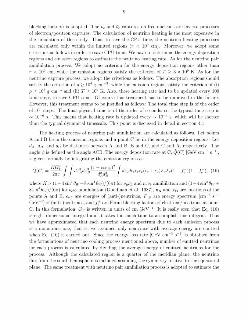
The heating process of neutrino pair annihilation are calculated as follows. Let points

A and B be in the emission regions and a point C be in the energy deposition regions. Let

dA, dB, and dC be distances between A and B, B and C, and C and A, respectively. The

angle ψ is defined as the angle ACB. The energy deposition rate at C, Q(C) [GeV cm−3 s−1],

is given formally by integrating the emission regions as

Q(C) =KG2

F

2πc

∫ ∫

dx3Adx

3B

(1 − cosψ)2

d2Ad

2B

∫

dενdενενεν(εν + εν)FνFν(1 − f−e )(1 − f+

e ), (16)

where K is (1−4 sin2 θW +8 sin4 θW )/(6π) for νµνµ and ντντ annihilation and (1+4 sin2 θW +

8 sin4 θW )/(6π) for νeνe annihilation (Goodman et al. 1987), xA and xB are locations of the

points A and B, εν,ν are energies of (anti-)neutrinos, Fν,ν are energy spectrum [cm−3 s−1

GeV−1] of (anti-)neutrinos, and f±e are Fermi blocking factors of electrons/positrons at point

C. In this formulation, GF is written in units of cm GeV−1. It is easily seen that Eq. (16)

is eight dimensional integral and it takes too much time to accomplish this integral. Thus

we have approximated that each neutrino energy spectrum due to each emission process

is a monotonic one, that is, we assumed only neutrinos with average energy are emitted

when Eq. (16) is carried out. Since the energy loss rate [GeV cm−3 s−1] is obtained from

the formulations of neutrino cooling process mentioned above, number of emitted neutrinos

for each process is calculated by dividing the average energy of emitted neutrinos for the

process. Although the calculated region is a quarter of the meridian plane, the neutrino

flux from the south hemisphere is included assuming the symmetry relative to the equatorial

plane. The same treatment with neutrino pair annihilation process is adopted to estimate the

– 10 –

heating rate due to νe and νe capture processes, that is, average energy of (anti-)electron-type

neutrinos is used.

Neutrinos are emitted isotropically in the fluid-rest frame, so strictly speaking, neutrinos

are emitted unisotropically in the coordinate system due to the beaming effect (Rybicki and Lightman 1979).

In fact, the angular frequency is found to become as large as 104 s−1 at the inner most region

(Figs. 3 and 10) and the rotation velocity, vφ reaches ∼ 1010 cm s−1 at most. Thus the

beaming effect may be important although we did not take into account the effect in this

study.

Finally the models considered in this study are summarized in Table 1. The digit in the

name of each model represents the power index of B0.

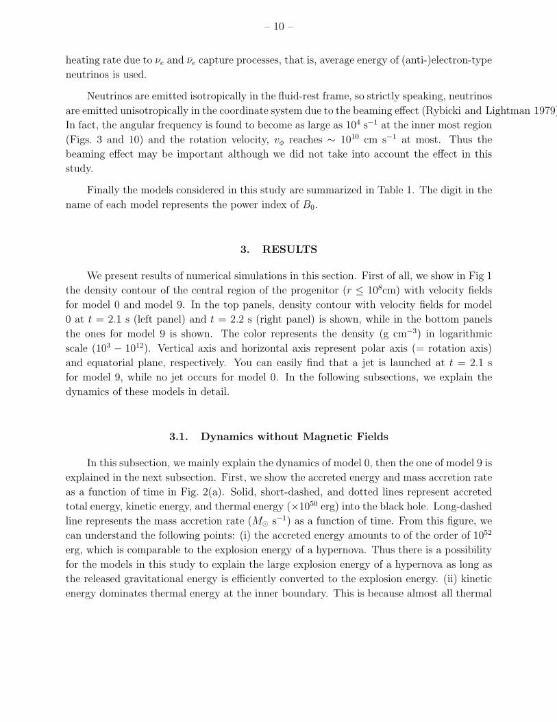
3. RESULTS

We present results of numerical simulations in this section. First of all, we show in Fig 1

the density contour of the central region of the progenitor (r ≤ 108cm) with velocity fields

for model 0 and model 9. In the top panels, density contour with velocity fields for model

0 at t = 2.1 s (left panel) and t = 2.2 s (right panel) is shown, while in the bottom panels

the ones for model 9 is shown. The color represents the density (g cm−3) in logarithmic

scale (103 − 1012). Vertical axis and horizontal axis represent polar axis (= rotation axis)

and equatorial plane, respectively. You can easily find that a jet is launched at t = 2.1 s

for model 9, while no jet occurs for model 0. In the following subsections, we explain the

dynamics of these models in detail.

3.1. Dynamics without Magnetic Fields

In this subsection, we mainly explain the dynamics of model 0, then the one of model 9 is

explained in the next subsection. First, we show the accreted energy and mass accretion rate

as a function of time in Fig. 2(a). Solid, short-dashed, and dotted lines represent accreted

total energy, kinetic energy, and thermal energy (×1050 erg) into the black hole. Long-dashed

line represents the mass accretion rate (M s−1) as a function of time. From this figure, we

can understand the following points: (i) the accreted energy amounts to of the order of 1052

erg, which is comparable to the explosion energy of a hypernova. Thus there is a possibility

for the models in this study to explain the large explosion energy of a hypernova as long as

the released gravitational energy is efficiently converted to the explosion energy. (ii) kinetic

energy dominates thermal energy at the inner boundary. This is because almost all thermal

– 11 –

energy is extracted in the form of neutrinos, which is seen in Fig. 6(a). (iii) mass accretion

rate drops almost monotonically from ∼ 10−1M s−1 to ∼ 10−3M s−1, which is discussed

in sections 3.2 and 4.2.

Next, we show in Fig. 3 profiles of physical quanta of the accretion disk around the

equatorial plane. Profiles of density, absolute value of radial velocity, angular frequency,

temperature, density scale height, and specific angular momentum in the accretion disk are

shown for model 0 at t = 2.2 s. From the figure, we can understand the following points: (i)

the density reaches as high as 1012 g cm−3 around the central region. (ii) the inflow velocity

(vr) becomes as low as 106 cm s−1 at the central region, by which the mass accretion rate

becomes as low as 10−3M s−1, as shown in Fig. 2(a) (Note that the mass accretion mainly

comes from the region between the rotational axis and the disk. See also Igumenshchev and

Abramowicz 2000; Proga and Begelman 2003).

We show in Fig. 4 profiles of mass fraction for nuclear elements at the equatorial plane

for model 0 at t = 2.2 s. Dot-dashed, dotted, short-dashed, long-dashed, and solid lines

represent mass fraction of n, p, 4He, 16O, and 56Ni, respectively. From this figure, we can

easily see that oxygen is photo-dissociated into helium at 2× 108cm, while helium is photo-

dissociated into nucleons at 3× 107cm. It is also noted, some 56Ni is seen at r ≤ 3× 107 cm

(solid line), which may explain the luminosity of a hypernova as long as it is ejected. This

point is discussed in section 4.3. The discontinuity of temperature at 3 × 107 cm in Fig. 3

will come from the cooling effect due to the photo-disintegration of helium into nucleons.

From now on we show the results on neutrino processes. In Fig. 5, we show contour

of neutrino cooling rate with velocity fields for model 0 at t = 2.2 s. The color represents

the emissivity of neutrinos (erg cm−3 s−1) in logarithmic scale (1010 − 1034). This emissivity

of neutrinos is almost explained by pair-captures on free nucleons, as shown in Fig. 6. We

can easily see that emissivity of neutrinos is high at the region where the accretion disk is

formed.

We show the results on neutrino cooling for every neutrino process. We show in Fig. 6(a)

cumulative energy (×1050 erg) of emitted neutrinos for each process as a function of time for

model 0. Dot-dashed, long-dashed, solid, short-dashed, and dotted lines represent plasmon

decay, electron-positron pair annihilation, positron capture, electron capture, and summation

of all processes. It is clearly seen that almost all emitted energy comes from pair captures on

free nucleons. Also, the emitted energy amounts to of the order of 1052 erg (strictly speaking,

3.44×1052erg), which is comparable to the accreted kinetic energy and much higher than the

accreted thermal energy (see Fig. 2(a)). Thus we consider that almost all thermal energy,

which was comparable to the kinetic energy in the accretion disk, is extracted by neutrino

emission. Note that time evolution of electron fraction is mainly determined by positron and

– 12 –

electron capture processes in the accretion disk.

In Fig. 7, we show contour of neutrino heating rate with velocity fields for model 0 at t

= 2.2 s. The color represents the energy deposition rate (erg cm−3 s−1) in logarithmic scale

(1010 − 1034). Left panel shows the energy deposition rate due to νe and νe captures on free

nucleons, while right panel shows the energy deposition rate due to ν and ν pair annihilation.

In the pair annihilation, contributions from three flavors are taken into account. It is, of

course, that contour of energy deposition rate due to νe and νe captures traces the number

density of free nucleons, so the energy deposition rate is high around the equatorial plane

where the accretion disk is formed. On the other hand, energy deposition rate due to ν and ν

pair annihilation occurs everywhere, including the region around the polar axis. This feature

will be good to launch a jet along the polar axis, as pointed by MacFadyen and Woosley

(1999). However, this heating effect is too low to launch a jet in this study (see Fig. 1).

In Fig. 8(a), we show neutrino luminosity (solid line), energy deposition rate due to ν

and ν pair annihilation (dotted line), and energy deposition rate due to νe and νe captures

on free nucleons (dashed line) as a function of time for model 0. It is clearly seen that energy

deposition rate is much smaller than the neutrino luminosity, which supports our assumption

that the system is almost optically thin to neutrinos. Also, we can see that νe and νe captures

on free nucleons dominates ν and ν pair annihilation process as the heating process. It is

also noted that neutrino luminosity and energy deposition rate decreases along with time,

which reflects that the mass accretion rate also decreases along with time (Fig. 2(a)).

Finally, we show in Fig. 9(a) the integrated deposited energy (×1050 erg ) due to ν

and ν pair annihilation (solid line) and νe and νe captures on free nucleons (dashed line)

as a function of time. It is confirmed that νe and νe captures on free nucleons dominate

ν and ν pair annihilation process as the heating process. However, as shown in Figs. 5

and 7, νe and νe captures on free nucleons occur mainly in the accretion disk, where neutrino

cooling effect dominates neutrino heating effect. Thus νe and νe captures on free nucleons

is not considered to work for launching a jet. As for the ν and ν pair annihilation process,

although this process deposit energy everywhere, including the region around the polar axis,

the deposited energy amounts to only of the order of 1049 erg. This is 10−3 times smaller

than the explosion energy of a hypernova. In fact, as shown in Fig. 1, the jet is not launched

in model 0. Thus we conclude that the efficiency of neutrino heating is too low to launch a

jet in this study.

– 13 –

3.2. Dynamics with Magnetic Fields

In this subsection, we explain the dynamics of model 9 as an example of a collapsar

with magnetic fields. Dependence of dynamics on the initial amplitude of magnetic fields is

shown in section 3.3.1.

First, the accreted energy and mass accretion rate as a function of time are shown in

Fig. 2(b). The meaning of each line is same with Fig. 2(a), although dot-dashed line, which

is not in Fig. 2 (a), represents accreted electro-magnetic energy (×1050 erg) into the black

hole as a function of time. The reason why the final time of the simulation for model 9 is

2.23 s is that the amplitude of the magnetic field (in particular, Bφ) becomes so high at the

inner most region that the Alfven crossing time at the region make the time step extremely

small. Also, it seems that the mass accretion rate does not decrease so much in model 9.

Rather, it seems to keep ∼ 0.05M s−1. We guess this is because magnetic fields play a role

to transfer the angular momentum from inner region to outer region, which makes matter

fall into the black hole more efficiently. This point is also discussed with Figs. 8—12.

Next, we show in Fig. 10 profiles of physical quanta of the accretion disk around the

equatorial plane for model 9 at t = 2.2 s. When we compare these profiles with the ones in

Fig. 3, we can see that the radial velocity is higher in model 9 at small radius. This may

reflect that the mass accretion rate is higher in model 9 than model 0 (as stated in section

3.1, the mass accretion mainly comes from the region between the rotational axis and the

torus. So we have to note that this feature does not explain the mass accretion rate directly.

see also Fujimoto et al. 2006). As for the other profiles, there seems no significant difference

between the two models.

In Fig. 11, we show profiles of amplitude of magnetic fields as a function of radius on

the equatorial plane for model 9 at t = 2.2 s. Dotted, solid, and dashed lines represent

the amplitude of Br, Bθ, and Bφ, respectively. It is clearly seen that Bφ dominates within

r = 108cm. Thus we can conclude that magnetic pressure from Bφ drives the jet along the

rotation axis (see Fig. 1). This point is also discussed with Figs. 13—15. Also, these magnetic

fields may play a role to transfer the angular momentum. Since the viscosity parameter α

can be estimated as (Balbus & Hawley 1998; Akiyama et al. 2003)

α ∼ BrBφ

4πP, (17)

we plot in Fig. 11 the estimated viscosity parameter (×10−20) (long-dashed line). This figure

suggests that α-viscosity coming from the magnetic fields may play a role to transfer the

angular momentum at inner most region effectively. However, the angular momentum cannot

be transfered to infinity along the radial direction. This is confirmed by the Alfven Mach

– 14 –

number (×10−10) in the radial direction (≡ vr/vr,A; dot-dashed line in Fig. 11). At only

the inner most region, the flow becomes marginally sub-Alfvenic where the viscous force

due to magnetic stress can bring the angular momentum outward. Thus we consider that

the outflow (including the jet) in the polar direction (see Fig. 1 bottom) should bring the

angular momentum from the inner most region.

As additional information, we found that the velocity of the slow magnetiosonic wave is

almost same with the Alfven velocity. On the other hand, we found that the fluid is subsonic

against the fast magnetiosonic wave in the simulated region.

We show in Fig. 12 the profiles of specific angular momentum (cm2 s−1) on the equatorial

plane for model 0 (dotted line) and model 9 (short-dashed line) at t = 2.2 s. The profiles of

angular momentum density (g cm−1 s−1) for model 0 (long-dashed line) and model 9 (solid

line) are also shown in the figure. We confirmed that the specific angular momentum is

not so different between model 0 and model 9, but it is found that the angular momentum

density is lower in model 9 compared with model 0 at the inner region. This feature might

reflect that the matter falls into the black hole efficiently in model 9 at small radius (see

Fig. 11). This picture seems to be consistent with the almost constant accretion rate in

model 9 (Figs. 2(b)).

Cumulative energy (×1050 erg) of emitted neutrinos for each process as a function of

time for model 9 is shown in Fig. 6(b), neutrino luminosity, energy deposition rate due to ν

and ν pair annihilation, and energy deposition rate due to νe and νe captures on free nucleons

as a function of time for model 9 are shown in Fig. 8(b), and integrated deposited energy due

to ν and ν pair annihilation and νe and νe captures on free nucleons as a function of time for

model 9 are shown in Fig. 9(b) The meaning of each line in each figure is same with the one

used for model 0. We can derive a similar conclusion for the role of neutrino heating effect

in model 9 as in model 0. As for the νe and νe captures on free nucleons, the cumulative

deposited energy becomes as high as 1052 ergs that is comparable to the explosion energy of a

hypernova. However, this heating process occurs mainly in the accretion disk, where neutrino

cooling effect dominates neutrino heating effect. Thus νe and νe captures on free nucleons is

not considered to work for launching a jet. As for the ν and ν pair annihilation process, the

deposited energy amounts to no more than 1050 erg. Thus we conclude that the neutrino

heating effect in model 9 is too inefficient to launch a GRB jet and cause a hypernova. It has

to be noted that the energy deposition rate due to pair captures on free nucleon sometimes

becomes larger than the neutrino luminosity in Fig. 8(b). This means that the optically

thin limit breaks down at that time. This point is also discussed in section 4.1. We also

found that the neutrino luminosity, energy deposition rate, and integrated deposited energy

seem to be higher in model 9 than in model 0. We consider that this feature comes from

– 15 –

the high mass accretion rate (high rate of release of gravitational energy) caused by angular

momentum transfer due to magnetic fields.

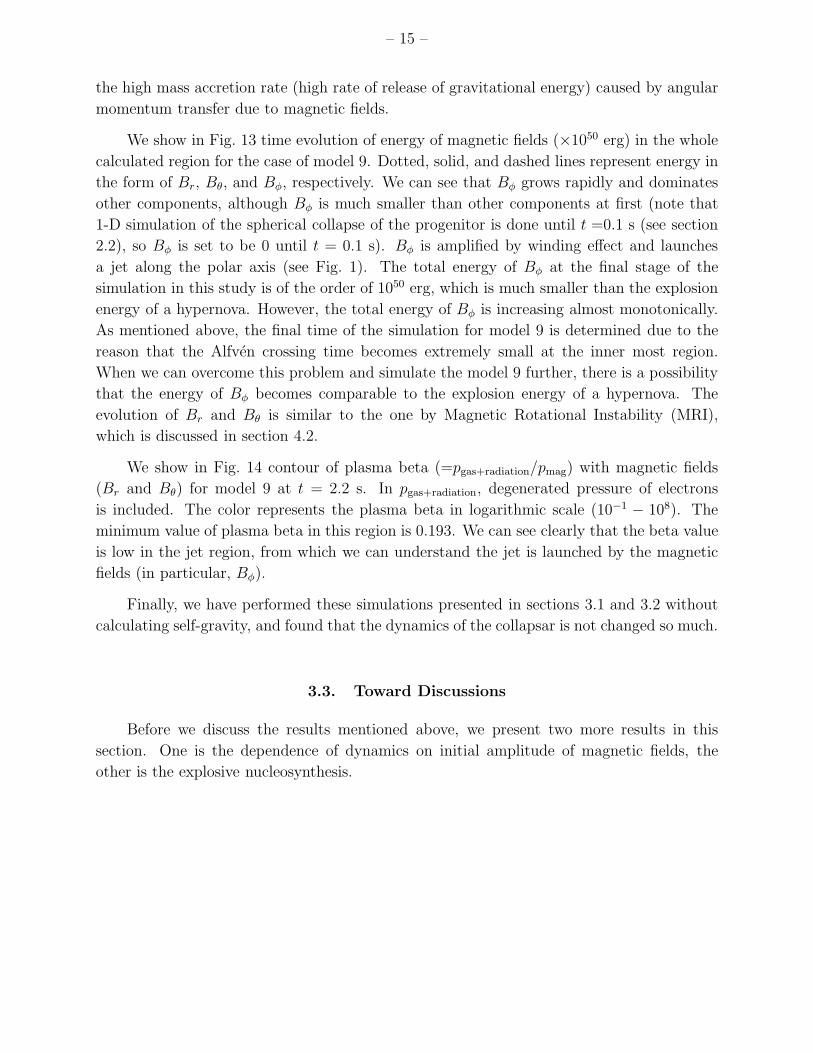
We show in Fig. 13 time evolution of energy of magnetic fields (×1050 erg) in the whole

calculated region for the case of model 9. Dotted, solid, and dashed lines represent energy in

the form of Br, Bθ, and Bφ, respectively. We can see that Bφ grows rapidly and dominates

other components, although Bφ is much smaller than other components at first (note that

1-D simulation of the spherical collapse of the progenitor is done until t =0.1 s (see section

2.2), so Bφ is set to be 0 until t = 0.1 s). Bφ is amplified by winding effect and launches

a jet along the polar axis (see Fig. 1). The total energy of Bφ at the final stage of the

simulation in this study is of the order of 1050 erg, which is much smaller than the explosion

energy of a hypernova. However, the total energy of Bφ is increasing almost monotonically.

As mentioned above, the final time of the simulation for model 9 is determined due to the

reason that the Alfven crossing time becomes extremely small at the inner most region.

When we can overcome this problem and simulate the model 9 further, there is a possibility

that the energy of Bφ becomes comparable to the explosion energy of a hypernova. The

evolution of Br and Bθ is similar to the one by Magnetic Rotational Instability (MRI),

which is discussed in section 4.2.

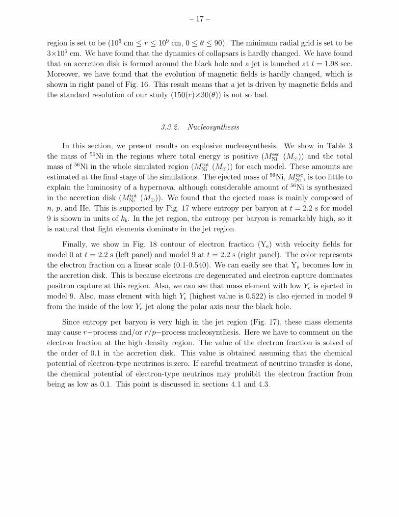
We show in Fig. 14 contour of plasma beta (=pgas+radiation/pmag) with magnetic fields

(Br and Bθ) for model 9 at t = 2.2 s. In pgas+radiation, degenerated pressure of electrons

is included. The color represents the plasma beta in logarithmic scale (10−1 − 108). The

minimum value of plasma beta in this region is 0.193. We can see clearly that the beta value

is low in the jet region, from which we can understand the jet is launched by the magnetic

fields (in particular, Bφ).

Finally, we have performed these simulations presented in sections 3.1 and 3.2 without

calculating self-gravity, and found that the dynamics of the collapsar is not changed so much.

3.3. Toward Discussions

Before we discuss the results mentioned above, we present two more results in this

section. One is the dependence of dynamics on initial amplitude of magnetic fields, the

other is the explosive nucleosynthesis.

– 16 –

3.3.1. Dependence on Initial Amplitude of Magnetic Fields and on Resolution of Grids

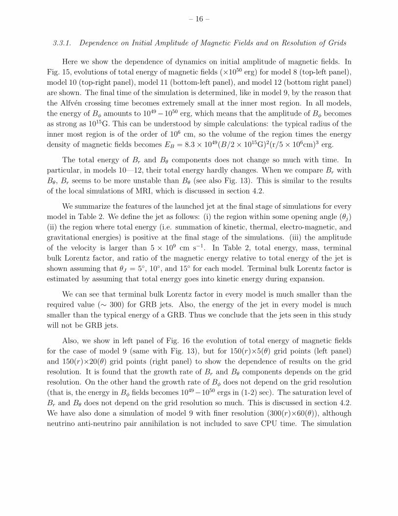
Here we show the dependence of dynamics on initial amplitude of magnetic fields. In

Fig. 15, evolutions of total energy of magnetic fields (×1050 erg) for model 8 (top-left panel),

model 10 (top-right panel), model 11 (bottom-left panel), and model 12 (bottom right panel)

are shown. The final time of the simulation is determined, like in model 9, by the reason that

the Alfven crossing time becomes extremely small at the inner most region. In all models,

the energy of Bφ amounts to 1049−1050 erg, which means that the amplitude of Bφ becomes

as strong as 1015G. This can be understood by simple calculations: the typical radius of the

inner most region is of the order of 106 cm, so the volume of the region times the energy

density of magnetic fields becomes EB = 8.3 × 1049(B/2 × 1015G)2(r/5 × 106cm)3 erg.

The total energy of Br and Bθ components does not change so much with time. In

particular, in models 10—12, their total energy hardly changes. When we compare Br with

Bθ, Br seems to be more unstable than Bθ (see also Fig. 13). This is similar to the results

of the local simulations of MRI, which is discussed in section 4.2.

We summarize the features of the launched jet at the final stage of simulations for every

model in Table 2. We define the jet as follows: (i) the region within some opening angle (θj)

(ii) the region where total energy (i.e. summation of kinetic, thermal, electro-magnetic, and

gravitational energies) is positive at the final stage of the simulations. (iii) the amplitude

of the velocity is larger than 5 × 109 cm s−1. In Table 2, total energy, mass, terminal

bulk Lorentz factor, and ratio of the magnetic energy relative to total energy of the jet is

shown assuming that θJ = 5, 10, and 15 for each model. Terminal bulk Lorentz factor is

estimated by assuming that total energy goes into kinetic energy during expansion.

We can see that terminal bulk Lorentz factor in every model is much smaller than the

required value (∼ 300) for GRB jets. Also, the energy of the jet in every model is much

smaller than the typical energy of a GRB. Thus we conclude that the jets seen in this study

will not be GRB jets.

Also, we show in left panel of Fig. 16 the evolution of total energy of magnetic fields

for the case of model 9 (same with Fig. 13), but for 150(r)×5(θ) grid points (left panel)

and 150(r)×20(θ) grid points (right panel) to show the dependence of results on the grid

resolution. It is found that the growth rate of Br and Bθ components depends on the grid

resolution. On the other hand the growth rate of Bφ does not depend on the grid resolution

(that is, the energy in Bφ fields becomes 1049−1050 ergs in (1-2) sec). The saturation level of

Br and Bθ does not depend on the grid resolution so much. This is discussed in section 4.2.

We have also done a simulation of model 9 with finer resolution (300(r)×60(θ)), although

neutrino anti-neutrino pair annihilation is not included to save CPU time. The simulation

– 17 –

region is set to be (106 cm ≤ r ≤ 109 cm, 0 ≤ θ ≤ 90). The minimum radial grid is set to be

3×105 cm. We have found that the dynamics of collapsars is hardly changed. We have found

that an accretion disk is formed around the black hole and a jet is launched at t = 1.98 sec.

Moreover, we have found that the evolution of magnetic fields is hardly changed, which is

shown in right panel of Fig. 16. This result means that a jet is driven by magnetic fields and

the standard resolution of our study (150(r)×30(θ)) is not so bad.

3.3.2. Nucleosynthesis

In this section, we present results on explosive nucleosynthesis. We show in Table 3

the mass of 56Ni in the regions where total energy is positive (M escNi (M)) and the total

mass of 56Ni in the whole simulated region (M totNi (M)) for each model. These amounts are

estimated at the final stage of the simulations. The ejected mass of 56Ni, M escNi , is too little to

explain the luminosity of a hypernova, although considerable amount of 56Ni is synthesized

in the accretion disk (M totNi (M)). We found that the ejected mass is mainly composed of

n, p, and He. This is supported by Fig. 17 where entropy per baryon at t = 2.2 s for model

9 is shown in units of kb. In the jet region, the entropy per baryon is remarkably high, so it

is natural that light elements dominate in the jet region.

Finally, we show in Fig. 18 contour of electron fraction (Ye) with velocity fields for

model 0 at t = 2.2 s (left panel) and model 9 at t = 2.2 s (right panel). The color represents

the electron fraction on a linear scale (0.1-0.540). We can easily see that Ye becomes low in

the accretion disk. This is because electrons are degenerated and electron capture dominates

positron capture at this region. Also, we can see that mass element with low Ye is ejected in

model 9. Also, mass element with high Ye (highest value is 0.522) is also ejected in model 9

from the inside of the low Ye jet along the polar axis near the black hole.

Since entropy per baryon is very high in the jet region (Fig. 17), these mass elements

may cause r−process and/or r/p−process nucleosynthesis. Here we have to comment on the

electron fraction at the high density region. The value of the electron fraction is solved of

the order of 0.1 in the accretion disk. This value is obtained assuming that the chemical

potential of electron-type neutrinos is zero. If careful treatment of neutrino transfer is done,

the chemical potential of electron-type neutrinos may prohibit the electron fraction from

being as low as 0.1. This point is discussed in sections 4.1 and 4.3.

– 18 –

4. DISCUSSIONS

In this section, we discuss our numerical results and prospect for future works. We

discuss neutrino physics, effects of magnetic fields, nucleosynthesis, general relativistic effects,

initial conditions, and prospect for improvements of our numerical code.

4.1. Neutrino Physics

In this study, we found that deposited energy due to neutrino pair annihilation are too

small to explain the explosion energy of a hypernova and a GRB (Fig. 9). Even though

the deposited energy by electron-type neutrino capture on free nucleons can be comparable

to the explosion energy of a hypernova in model 9 (Fig. 9), the deposition region is the

high density region (Fig. 7) where cooling effect dominates the heating effect (Fig. 5). In

particular, no jet was found in the numerical simulations of model 0 (Fig. 1). The energetics

of this system can be understood from Figs. 2, 6, and 9. The released gravitational energy

by collapse is the energy source of accreted energy and neutrinos. From Figs. 2 and 6, we

can understand that the kinetic energy and thermal energy share the released gravitational

energy almost equally, then almost thermal energy was extracted in the form of neutrinos.

The total energies of accreted energy and neutrinos are of the order of 1052 erg, then the

emitted neutrino energy was deposited into matter through weak interactions. Its efficiency

is less than 1% for neutrino pair annihilation, as can be seen in Figs. 6 and 9. As for the

efficiency of electron-type neutrino capture it amounts to ∼ 10 − 20%. This means that

the inner most region of the accretion disk becomes to optically thick against neutrinos and

∼ 10 − 20% of neutrinos are absorbed.

The deposited energy by neutrino pair annihilation is of the order of (1049 − 1050 erg,

which is much smaller than the explosion energy of a hypernova and a GRB. In order to

enhance the deposited energy by neutrino pair annihilation, there will be two ways. One

is to enhance the released gravitational energy, the other is to enhance the efficiency of

energy deposition. The former corresponds to enhance the mass accretion rate, which will

be realized if effective angular momentum transfer is realized. From Figs. 2, 8, and 12, it

was inferred that magnetic fields seem to work efficiently so that high mass accretion rate

is realized. Of course, the mass accretion rate also depends on the distribution of initial

angular momentum. We should investigate these effects further in the future. As for the

efficiency of energy deposition, it will be enhanced when the general relativistic effects are

taken into account. This is because neutrinos are trapped around the black hole, so that the

possibilities of neutrino pair annihilation and neutrino capture become enhanced. This effect

is investigated in detail by using a steady solution of an accretion disk in the forth-coming

– 19 –

paper. Of course, we are planning to include this effect in our numerical code in the future.

Although we believe that our conclusion on the energetics mentioned above will be

unchanged, we have to improve our treatment on the neutrino heating for further study. In

this study, we took the optical thin limit to estimate the neutrino heating rate. This will

be justified by Figs. 6 and 9. However, for further study, we have to investigate the cases in

which mass accretion rate is higher than in this study to achieve energetic explosion enough

to explain the explosion energies of a hypernova and a GRB. In fact, we consider that the

optically thin limit breaks down even the models in this study at the highest density region.

This is estimated as follows: The cross section of νe and νe captures on free nucleons is given

by σ ∼ σ0(εν/mec2)2 where σ0 = 1.76×10−44 cm2. Since the highest density in the accretion

disk is of the order of 1012 g cm−3 at r ∼ 106 cm (the scale hight is also of the order of

106cm) and typical energy of neutrinos are of the order of 10 MeV (see Figs. 3 and 10), the

optical depth at this region is τ = σ(ρ/mp)L ∼ 4.2(εν/10MeV)2(ρ/1012g cm−3)(L/106cm).

Thus, at the highest density region, the optically thin limit must break down. This picture is

also confirmed in Fig. 8(b). In Fig. 8(b), as stated in section 3.2, the energy deposition rate

due to pair captures on free nucleon sometimes becomes larger than the neutrino luminosity.

This reflects that the optically thin limit breaks down at that time. Although we believe that

our conclusion on the energetics will not be changed so much, we are planning to develop

the careful neutrino transfer code that includes emissions, absorptions, and scattering of

neutrinos for further study. We also note four points that have to be improved for the

treatments of neutrino heating. One is that we did not take into account the light-crossing

time of the system and assumed that the system is almost steady during the light-crossing

time when we estimate the neutrino heating rate. From Figs. 5 and 7, the neutrino cooling

and heating occur efficiently within several times of 107cm. Thus the typical light crossing

time will be of the order of 1ms. For comparison, the rotation period at the inner most region

is ∼ 6.3 × 10−4 s. Since the system forms an accretion disk and the viscosity parameter α

is 0.1 at most (Fig. 11), the system will be treated steady at least ten times of the rotation

period, 6.3 × 10−3 s. Thus the treatment to neglect the light crossing time will be fairly

justified. Second is that we update the neutrino heating rate every 100 timesteps to save

the CPU time. The inner most radius is set to be 106 cm, so the typical time step is

estimated to be 106 × ∆θ/c s, where c is the speed of light and ∆θ = π/60. Thus 100

time steps corresponds to 1.74 ∼ 10−4 s, which will be comparable to free-fall timescale

(τff = 1/√

24πGρ ∼ 4.5 × 10−4(1012g cm−3/ρ)1/2 s (Woosley 1986)) and rotation period.

Thus we believe that this treatment will be fairly justified. Third, we have approximated

that each neutrino energy spectrum due to each emission process is monotonic, that is,

we assumed only neutrinos with average energy are emitted when Eq. (16) is carried out.

However, the cross section of neutrino pair annihilation is proportional to square of the total

– 20 –

energy in the center of mass, and that for electron-type neutrino absorption on free nucleons

is proportional to square of neutrino’s energy. Thus the contribution of neutrinos with

high energy will enhance the efficiency of neutrino heating. These points will be improved

when we can include a careful neutrino transfer code in future. The last point is related

with the nuclear reactions. In this study, the NSE was assumed for the region where T ≥5 × 109 [K]. Thus, the reactions to maintain NSE occur suddenly when the temperature

becomes so high as to satisfy the criterion. However, in reality, NSE might break down at

low density region, where cooling effect due to photo-disintegration will be not so strong

as in this simulation. It should be also noted that the photo-dissociation from He into

nucleons is strong cooling effect and absorb thermal energy when this reaction is switched

on. Thus the thermal energy suddenly absorbed by nuclear reactions. That is seen as the

discontinuities of temperature in Figs. 3 and 10. Although we believe these discontinuities do

not change our conclusion on the energetics mentioned above (because much more neutrinos

come from the inner region; Fig. 5), the profile of temperature will be solved smoothly when

we use a nuclear reaction network instead of using the NSE relation. Since the emissivity

of neutrinos depends very sensitively on the temperature (Bethe 1990; Herant et al. 1992;

Lee & Ramirez-Ruiz 2006), estimation of temperature should be treated carefully. We are

planning to check the dependence of temperature on the nuclear reaction network and several

EOS in the forth coming paper.

Finally, we discuss the detectability of neutrinos from collapsars. Since the event rate is

much smaller than the normal core-collapse supernova, the chance probability to detect neu-

trino signals from a collapsar will be very small. However, if it occurs nearby our galaxy, the

neutrino signal from a collapsar will be distinguished from normal core-collapse supernova.

As for the normal core-collapse supernovae, the time evolution of the luminosity of neutrino

of each flavor is determined firmly by the binding energy of a neutron star and opacity of

neutron star against neutrinos. On the other hand, in the case of a collapsar, the time

evolution of neutrino luminosity will depend on the time evolution of mass accretion rate,

which in turn should depend on the initial distribution of angular momentum and magnetic

fields. Thus there should be much varieties of time evolution for the luminosity of neutrinos

in the case of collapsars. Also, in the case of collapsars, the dominant process to generate

neutrinos is pair captures on free nucleons (see Fig. 6), so in the case of a collapsar, the

electron-type neutrinos will be much more produced compared with other flavors. This is in

contrast with the normal core-collapse supernovae(e.g. Buras et al. 2006, and see references

therein). Of course, we have to take vacuum and matter oscillation effects into account to

estimate the spectrum of neutrinos from a collapsar precisely. In particular, in the case of a

collapsar, the density distribution is far from spherically symmetric, so we have to be careful

about viewing angle to estimate the matter oscillation effect. It is true that the event rate

– 21 –

of collapsars is smaller than normal core collapse supernovae, but the released gravitational

energy can be larger if considerable amount of mass of the progenitor falls into the central

black hole (Nagataki et al. 2002). Thus we consider that there will be also a possibility to

detect a neutrino background from collapsars.

4.2. Effects of Magnetic Fields

We have seen that the mass accretion rate seems to be enhanced in model 9, compared

with model 0 (Fig. 2), which enhances the luminosity of neutrinos (Fig. 6) and energy depo-

sition rate due to weak interactions (Fig. 8). This seems to be because magnetic viscosity is

effective at inner most region (Fig. 11 and Fig. 12) and multi-dimensional outflow (Fig. 1)

carries angular momentum outward. Thus amplification of magnetic fields is important not

only for launching a jet by magnetic pressure, but also for enhancing mass accretion rate and

energy deposition rate through weak interactions. In our study, we assume the axisymmetry

of the system to save CPU time. In this case, the field built up by the effect of magnetoro-

tational instability (MRI) decays due to Cowling’s anti-dynamo theorem (Shercliff 1965).

However, the plasma beta becomes lower than unity in the jet region (Fig. 14), which is

embodied by the amplification of Bφ fields (Figs. 13 and 15). Thus we consider that Bφ

field is not amplified by MRI effects, but by winding-up of poloidal fields due to differential

rotation. The typical timescale of winding-up at the inner most region will be (see Figs. 3

and 10)

τwind ∼ 2πd ln r

dΩ∼ 2π ln 10

104∼ 1.45 × 10−3 s. (18)

This timescale will correspond to the steep rising of energy of Bφ around t = 0.1 s in

Figs. 13 and 15. After the steep growth, when the strength of Bφ becomes comparable

to the poloidal component, the growth rate declines since Bφ grows by winding the ’weak’

poloidal component (Takiwaki et al. 2004). The final time of the simulation is determined

when the Alfven speed reaches to the order of the speed of light. This is understood as

follows: Alfven crossing time in the θ-direction at the innermost region becomes r∆θ/vA =

106 × (π/60)/c = 1.74×10−6s. Since the total timestep is several times of 106, the final time

is estimated to be several time, which is consistent with our results. The Alfven speed is

estimated to be

vA =B√4πρ

∼ 2.82 × 108

(

B

1015G

) (

1012g cm−3

ρ

)1/2

cm s−1 (19)

∼ 2.82 × 1010

(

B

1015G

) (

108g cm−3

ρ

)1/2

cm s−1, (20)

– 22 –

which means that the final time is determined not by the time when the amplitude of Bφ

reaches to 1015G around the equatorial plane, but by the time when the amplitude of Bφ

reaches to 1015G at low density region, that is, around the polar region where the jet is

launched.

As for Br and Bθ fields, from Fig. 13, some instabilities seem to grow and saturate,

which is similar to the behavior of MRI (Hawley & Balbus 1991; Balbus & Hawley 1998).

At present, we consider that these instabilities are MRI modes with a wavelength of maximum

growth mode unresolved. However, we can not conclude that these instabilities are really

unresolved MRI modes. This is due to the reason as follows: The dispersion relation of the

linear MRI modes is obtained analytically by assuming that the accretion disk is supported

by rotation (that is, in Kepler motion). On the other hand, as shown in Figs. 3 and 10, the

radial velocity is non-zero in the accretion disks in this study. Moreover, the radial flow speed

is super-slow magnetosonic (the speed of slow magnetosonic wave is almost same with that

of Alfven wave in this study: Fig. 11). Since MRI is the instability of the slow-magnetosonic

waves in a magnetized and differentially rotation plasma, the dispersion relation may be

changed considerably for such a super-slow magnetosonic flow. However, there is no analytic

solution for such a flow at present, so we use the dispersion relation of MRI for the discussion

here.

Ignoring entropy gradients, the condition for the instability of the slow-magnetosonic

waves in a magnetized, differentially rotation plasma is (Balbus & Hawley 1991)

dΩ2

d ln r+ (k · vA)2 < 0, (21)

where k is the vector of the wave number. The wavelength of maximum growth of the linear

instability is

λ0 =2πvA

Ω∼ 1.77 × 103

(

104s−1

Ω

) (

B

1013G

)(

1012g cm−3

ρ

)1/2

cm. (22)

Since λ0 is much smaller than the grid size of the inner most region (∆r = 3 × 105cm), the

linear MRI mode of maximum growth is not resolved in this study (note that the amplitudes

of Br and Bθ are of the order of 1013G and much smaller than Bφ; see Fig. 11). However, MRI

grows as long as Eq. (21) holds. Since the value of the first term of Eq. (21) at the inner most

region is ∼ −108/ ln 10 ∼ −4.34× 107, it is confirmed that inner most region is unstable for

MRI mode with the wave length longer than ∼ 103(B/1013G)(1012g cm−3/ρ)1/2cm. The char-

acteristic growing timescale is (Balbus & Hawley 1998; Akiyama et al. 2003; Proga et al. 2003)

τMRI ∼ 2π

∣

∣

∣

∣

dΩ2

d ln r

∣

∣

∣

∣

−1/2

∼ 6.74 × 10−4 s, (23)

– 23 –

which is seen in model 9 (Fig. 13) and model 8 (Fig. 15). The saturation level of Br seems to

be slightly higher than that of Bθ, which is similar to the results of the local simulations of

MRI (Sano et al. 2004). Also, as shown in Fig. 16, the growth rate of Br and Bθ components

depends on the grid resolution, while the growth rate of Bφ does not depend on the grid

resolution. In fact, the growth rate becomes smaller for a coarse mesh case (Fig. 16(a)).

This is similar to the picture that Br and Bθ are amplified by MRI, while Bφ is amplified

by winding effect. The saturation level of Br and Bθ seems not to be sensitive to the grid

resolution. As stated above, in order to prove firmly that Br and Bθ are amplified by MRI-

like instability, dispersion relation of linear growing modes for super-slow magnetosonic flow

has to be obtained analytically and the dispersion relation has to be reproduced by numerical

simulations with finer grid resolution, which is outscope of this study.

As shown in Fig. 11, the estimated viscosity parameter becomes larger than 10−3 at

almost all region in r ≤ 4 × 104 cm. Since the angular velocity becomes larger than 103 for

r ≤ 6 × 106 cm (Fig. 10), this viscosity becomes effective in a timescale of second, which

is comparable to our simulations. Thus we think this viscosity drives high mass accretion

rate in the models with magnetic fields. However, as stated in section 3.2, the angular

momentum cannot be transfered to infinity along the radial direction. As shown in Fig. 11,

the flow is super-Alfvenic except for the inner most region. Thus angular momentum cannot

be conveyed outward by Alfven wave in the radial direction. At present, we consider that

the outflow (including the jet) in the polar direction in model 9 should bring the angular

momentum from the inner most region (see Fig. 1 bottom). This picture is similar to

CDAF (Narayan et al. 2001). We are planning to present further analysis of this feature in

the forth-coming paper.

Since the plasma beta can be of the order of unity at the inner most region (Fig. 14)

and Bφ dominates Br and Bθ at the region (r ≤ 7 − 8 × 107cm), we can understand that

the magnetic pressure from Br and Bθ is much smaller than the radiation pressure (from

photons, electrons, and positrons) and degenerate pressure. Thus, the jet cannot be launched

by the effects of Br and Bθ only. The winding-up effect is necessary to amplify Bφ field so

that the magnetic pressure becomes comparable to the radiation and degenerate pressure.

We saw that MRI-like instability seems to occur from the beginning of the simulations (see

model 8 in Fig. 15). However, since the saturation level is not so high, the amplified energy

of magnetic fields for Br and Bθ cannot be seen well at first (see model 9 in Fig. 13 and model

10 in Fig. 15). This is because at the early phase the steady accretion disk is not formed

and released gravitational energy is not so much (see Fig. 2). In model 11 and model 12,

the initial total energies of magnetic fields are so high that the effect of MRI-like instability

cannot be seen (Fig. 15).

– 24 –

As stated above, the axisymmetry of the system is assumed in this study. So wind-

ing up effect only amplifies m = 0 mode of Bφ. Usually, it is pointed out that saturation

level of the winding up effects becomes lower when three dimensional simulations are per-

formed (Hawley et al. 1995). Thus Bφ may not be amplified as strong as 1015G. Also, at the

present study, the timescale for Bφ fields at the inner most region to be amplified to ∼ 1015G

depends on the initial amplitude of the magnetic fields (see Figs. 13 and 15). However, if

three dimensional simulations are performed, instabilities due to MRI(-like) modes do not

decay due to Cowling’s anti-dynamo theorem. Also, the MRI(-like) modes with wave vec-

tors whose φ components are non-zero, which amplify Bφ are included (Masada et al. 2006).

If such MRI(-like) modes that amplify Bφ are included, the dependence of the dynamics

on the initial amplitude of the magnetic fields may be diluted. We have to perform three

dimensional calculations to see what happens in more realistic situations.

As stated above, the timestep becomes so small when the Alfven crossing time becomes

so small. Since this calculation is Newtonian, the speed of light is not included in the basic

equations for macro physics (Eq. (1)-Eq. (6)). In fact, we found that the Alfven speed

becomes larger than the speed of light at some points by a factor of two or so at the final

stage of simulations. Thus it will be one of the solutions to overcome this problem is to

develop the special relativistic MHD code, in which the Alfven speed is, of course, solved to

be smaller than the speed of light.

In this study, we considered the ideal MHD without dissipation (it is, of course, numer-

ical viscosity is inevitably included due to finite gridding effects). When resistive heating

is efficient, considerable amount of energy in magnetic fields will be transfered to thermal

energy by ohmic-like dissipation and reconnection, which will change the dynamics of collap-

sars so much. The problem is, however, that the properties of resistivity of high density and

high temperature matter with strong magnetic fields are highly uncertain (it is noted that

artificial resistivity is included in Proga et al. (2003) in order to account of the dissipation

in a controlled way instead of allowing numerical effects to dissipate magnetic fields in an

uncontrolled manner (see also Stone and Pringle 2001)).

Finally, we discuss the total explosion energy and bulk Lorentz factor of the jet. From

Table 2, we can see that there seems to be a tendency that the mass of the jet becomes

heavier when the initial amplitude of the magnetic fields are stronger (model 10, model

11, and model 12), although this tendency is not monotonic (model 8 and model 9). This

will reflect that the jet is launched earlier and the density is still higher for a case with

stronger initial magnetic fields. There seems to be also tendency that the energy of the jet

becomes also larger when the initial amplitude of the magnetic fields is set to be stronger,

although this tendency is not also monotonic (model 8 and model 9). This tendency is not

– 25 –

so remarkable since the mass of the jet is heavier for a stronger magnetic field case and the

mass should have some amount of kinetic, thermal, and magnetic field energies. As for the

models 8 and 9, the information of initial condition might be lost considerably since it takes

much time to launch jets. From these results, we can conclude that no GRB jet is realized

even if strong magnetic fields is assumed. We consider that there will be a possibility that

a GRB jet is realized if we can perform numerical simulations for much longer physical time

(say, ∼ 10 − 100s). In such long timescale simulations, the energy of Bφ fields should be

much more than 1050 erg (see Figs. 13 and 15). Also, the density in the jet may become lower

along with time, because considerable mass will falls into the black hole along the polar axis.

Thus the terminal bulk Lorentz factor may be enhanced at later phase. In order to achieve

such a simulation, the special relativistic code will be helpful, as mentioned above.

4.3. Prospect for Nucleosynthesis

It is radioactive nuclei, 56Ni and its daughter nuclei, 56Co, that brighten the super-

nova remnant and determine its bolometric luminosity. 56Ni is considered to be synthesized

through explosive nucleosynthesis because its half-life is very short (5.9 days). Thus it is

natural to consider that explosive nucleosynthesis occurs in a hypernova that is accompanied

by a GRB. However, it is not clearly known where the explosive nucleosynthesis occurs (e.g.

Fryer et al. 2006a, Fryer et al. 2006b).

Maeda et al. (2002) have done a numerical calculation of explosive nucleosynthesis

launching a jet by depositing thermal and kinetic energy at the inner most region. They

have shown that a mass of 56Ni sufficient to explain the observation of hypernovae (∼ 0.5M)

can be synthesized around the jet region. In their calculation, all the explosion energy was

deposited initially. Thus Nagataki et al. (2006) investigated the dependence of explosive

nucleosynthesis on the energy deposition rate. They have shown that sufficient mass of56Ni can be synthesized as long as all the explosion energy is deposited initially, while the

synthesized mass of 56Ni is insufficient if the explosion energy is deposited for 10 s (that is,

the energy deposition rate is 1051 erg s−1). This is because matter starts to move outward

after the passage of the shock wave, and almost all of the matter moves away from the central

engine before the injection of thermal energy (= 1052 erg) is completed, so the amount of

mass where complete burning to synthesize 56Ni becomes little for such a long-duration

explosion (see also Nagataki et al (2003)).

On the other hand, it is pointed out the possibility that a substantial amount of 56Ni is

produced in the accretion disk and a part of it is conveyed outward by the viscosity-driven

wind by some authors (MacFadyen & Woosley 1999; Pruet et al. 2003). However, there is

– 26 –

much uncertainty how much 56Ni is ejected from the accretion disk. This problem depends

sensitively on the viscosity effects. Further investigation is required to estimate how much56Ni is ejected.

In this study, we have found that mass of 56Ni in the accretion disk (see Fig. 4) at the

final stage of simulations is of the order of 10−3M (M totNi in Table 3). Thus if considerable

fraction of the synthesized 56Ni is ejected without falling into the black hole, there will

be a possibility to supply sufficient amount of 56Ni required to explain the luminosity of a

hypernova. However, in the present study, the ejected mass of 56Ni was found to be only

10−11−10−6M (M escNi in Table 3). This is because the entropy per baryon in the jet is so high

(Fig. 17) that the light elements such as n, p, and He dominate in the jet. Thus we could not

show that sufficient mass of 56Ni was ejected from the accretion disk in the present study.

There will be two possibilities to extract enough amount of 56Ni from the accretion disk.

One is that 56Ni might be extracted efficiently from the accretion disk at later phase. Since

typical temperature of the accretion disk will be lower when the mass of the central black hole

becomes larger, the entropy per baryon in the jet will be decreased (Nagataki et al. 2002).

This feature should suggest that 56Ni dominates in the jet component at the late phase. The

other one is that some kinds of viscosities might work to convey the matter in the accretion

disk outward efficiently. In MacFadyen and Woosley (1999), they included α-viscosity and

showed that considerable amount can be conveyed. Since α viscosity is not included in

this study, such a feature was not seen. However, when three dimensional simulations with

higher resolution than in this study are done, much more modes of magnetic fields should

be resolved, and some of them might be responsible for viscosities and work like α-viscosity.

We discuss the possibility to synthesize heavy elements in collapsars. We have shown

that neutron-rich matter with high entropy per baryon is ejected along the jet axis (Figs. 17

and 18). This is because electron capture dominates positron capture in the accretion

disk (Fig. 6). Thus there is a possibility that r-process nucleosynthesis occurs in the

jet (Nagataki et al. 1997; Nagataki 2000; Nagataki 2001; Nagataki & Kohri 2001; Wanajo et al. 2002;

Suzuki & Nagataki 2005; Fujimoto et al. 2006). Moreover, we found that mass element with

high Ye (∼ 0.522) appears around the polar axis near the black hole. This is because νe cap-

ture dominates νe capture at the region. This is because flux of νe from the accretion disk

(note that νe comes from electron capture) is sufficiently large to enhance Ye at the region.

In such a high Ye region, there will be a possibility that r/p−process nucleosynthesis oc-

curs (Wanajo 2006). We are planning to perform such a numerical simulations in the very

near future. Also, there is a possibility that much neutrons are ejected from the jet since

the entropy per baryon amounts to the order of 104. If so, there may be a possibility that

signals from the neutron decays may be observed as the delayed bump of the light curve

of the afterglow (Kulukarni 2005) or gamma-rays (Razzaque & Meszaros 2006a). Also, GeV

– 27 –

emission may be observed by proton-neutron inelastic scattering (Meszaros & Rees 2000;

Rossi et al. 2006; Razzaque & Meszaros 2006b) Finally, note that a careful treatment of

neutrino transfer is important for the r- and r/p-process nucleosynthesis. As stated in sec-

tion 4.1, the optically thin limit may break down at the high density region. When the matter

becomes to be opaque to neutrinos, the neutrinos becomes to be trapped and degenerate. In

the high density limit, the chemical equilibrium is achieved as µe+µp = µn+µνewhere µe, µp,

µn, and µνeare chemical potentials of electrons, protons, neutrons, and electron-type neu-

trinos. When the chemical potential of electron-type neutrinos is not negligible, the electron

capture do not proceed further and electron fraction does not decrease so much (Sato 1975),

which should be crucial to the r- and r/p-process nucleosynthesis.

4.4. General Relativistic Effects

In this section, we discuss general relativistic effects that we are planning to include in

our magnetohydrodynamic simulation code.

First, we still believe that effects of energy deposition due to weak interactions (espe-

cially, neutrino anti-neutrino pair annihilation) can be a key process as the central engine

of GRBs. In fact, the temperature of the accretion disk becomes higher especially for a

Kerr black hole since the gravitational potential becomes deeper and much gravitational

energy is released at the inner most region and the radius of the inner most stable orbit

becomes smaller for a Kerr black hole (Popham et al. 1999; MacFadyen & Woosley 1999).

This effect will enhance the luminosity of the neutrinos from the accretion disk (Popham et

al. 1999), and the neutrino pair annihilation (Asano & Fukuyama 2000; Miller et al. 2003;

Kneller et al. 2006; Gu et al. 2006). In the vicinity of the black hole, most of neutrinos and

anti-neutrinos come shadows due to the bending effects of the neutrino geodesics. Since

the shape and position of the black hole shadow depend on the physical parameters of the

black hole (Bardeen 1973; Takahashi 2004, 2005), the effective area emitting the most of the

neutrino flux just outside of the black hole shadows is also determined by the black hole

parameters. These effects are included only when geodesics and disk structures are precisely

calculated.

Since according to our simulations the plasma beta (= pgas+radiation/pmag) in the

polar region is lower than the plasma beta in other regions and the minimum values of the

plasma beta is 0.193. This means that the polar region is magnetically dominated. In such

regions where the magnetic energy is dominated such as a force-free field, the extraction of the

rotational energy of the black hole is expected as Poynting flux (Blandford & Znajek 1977)

and the negative energy (Blandford & Payne 1982; Takahashi et al. 1990). Although these

– 28 –

effects have been confirmed numerically by many authors (Koide 2003; Mizuno et al. 2004b;

Komissarov 2005; Hawley & Krolic 2006; McKinney 2006), there are many unsolved issues

on the central engine of GRBs. Especially, the neutrino radiation from the negative energy

fluid in the realistic general relativistic accretion flow is one of the unsolved issue. The

past studies roughly estimate the extraction energy due to the Blandford-Znajek process to

become non-negligible amount to the explosion of the long GRSs (e.g. Lee et al. 2000a,

2000b; Di Matteo et al. 2002).

4.5. Variety of Initial Conditions

The properties of a progenitor of GRBs are still unknown. There are much uncertainties

on mass loss rate, final mass, angular momentum distribution, amplitude and configuration

of magnetic fields prior to collapse. These properties will depend not only on initial mass and

metallicity of progenitors but also on the presence (or absence) and properties of companion

stars (Maeder & Meynet 2001; Woosley & Heger 2006; MacFadyen et al. 2005). Thus it is

necessary to perform numerical simulations with many models of progenitors to ensure the

validity of the mechanism to launch a GRB jet from progenitors. In particular, we consider

that the initial angular momentum distribution should be important since the mass accretion

rate depends on it very sensitively.

4.6. Prospects for Improvements of Numerical Scheme

As shown in Eq. (22), the critical wavelength of maximum growth of the linear MRI

instability is quite short, so adaptive mesh refinement method (e.g. Norman 2005; Zhang

and MacFadyen 2006; Morsony et al. 2006) is inevitably required to resolve the critical

wavelength in a collapsar. Of course, much CPU time is required to perform three dimen-

sional calculation with adaptive mesh refinement method. Moreover, when we try to include

neutrino transfer code, three dimensions are required additionally for the momentum space.

However, people will be able to realize such an expensive simulation in the near future with

a help of rapidly growing power of super-computers. Of course, we are planning to devote

ourselves to developing such a numerical code.

– 29 –

5. SUMMARY AND CONCLUSION

We have performed two-dimensional magnetohydrodynamic simulations by the ZEUS-

2D code to investigate the dynamics of a collapsar that generates a GRB jet, taking account

of realistic equation of state (contribution of electrons, positrons, radiation, and ideal gas of

nuclei), neutrino cooling and heating processes, magnetic fields, and gravitational force from

the central black hole and self gravity.

We have found that neutrino heating processes (neutrino and anti-neutrino pair annihi-

lation, and νe and νe captures on free nucleons) are not so efficient to launch a jet. We have

found that a jet is launched by magnetic fields (in particular, Bφ fields that are amplified by

the winding-up effect). However, the ratio of total energy relative to the rest mass energy in

the jet at the final stage of simulations suggests that the bulk Lorentz factor of the jet will

not reach to as high as several hundred, so we conclude the jet seen in this study will not be

a GRB jet. We also found that the mass accretion rate seems to be enhanced in the models

with magnetic fields. This might be because angular momentum is efficiently transfered by

the viscosity due to the magnetic fields and multi-dimensional flow.

Since GRB jets are not obtained in this study, we consider that general relativistic ef-

fects, by which the efficiency of energy deposition through weak interactions will be enhanced

and rotation energy of the black hole will be transfered to matter through the magnetic fields,

will be important to generate a GRB jet. Thus we are planning to develop a general rela-

tivistic magnetohydrodynamics code in the very near future. Also, the accretion disk with

magnetic fields may still play an important role to launch a GRB jet, and it may be seen

if we can perform numerical simulations for much longer physical time (say, ∼ 10 − 100 s).

To realize such a simulation, the special relativistic code will be helpful because the Alfven

velocity is limited to the speed of light.

We have shown that considerable amount of 56Ni is synthesized in the accretion disk.

Thus if some fraction of the synthesized 56Ni is ejected without falling into the black hole,

there will be a possibility for the accretion disk to supply sufficient amount of 56Ni required

to explain the luminosity of a hypernova. Also, we have shown that neutron-rich matter with

high entropy per baryon is ejected along the rotation axis. This is because electron capture

dominates positron capture. Moreover, we found that the electron fraction becomes larger

than 0.5 around the polar axis near the black hole. This is because νe capture dominates

νe capture at the region. Thus there will be a possibility that r-process and r/p−process

nucleosynthesis occur at these regions. Finally, much neutrons will be ejected from the jet,

which suggests that signals from the neutron decays may be observed as the delayed bump

of the light curve of the afterglow or gamma-rays.

– 30 –

S.N. is grateful to S. Akiyama, R. Blandford, S. Fujimoto, S. Inutsuka, S. Mineshige, T.

Sano, S. Yamada, T. Yamasaki and M. Watanabe for useful discussion. The computation was

carried out on NEC SX-5 and SX-8, SGI Altix3700 BX2, and Compaq Alpha Server ES40 at

Yukawa Institute for Theoretical Physics, Kyoto University. This work is in part supported

by a Grant-in-Aid for the 21st Century COE “Center for Diversity and Universality in

Physics” from the Ministry of Education, Culture, Sports, Science and Technology of Japan.

S.N. is partially supported by Grants-in-Aid for Scientific Research from the Ministry of

Education, Culture, Sports, Science and Technology of Japan through No. 16740134. R.T.

is partially supported by Japan Society for the Promotion of Science No. 1710519. T.T is

partially supported by Japan Society for the Promotion of Science.

REFERENCES

Akiyama, S., et al. 2003, ApJ, 584, 954

Aloy, M.A., et al. 2000, ApJ, 531, L119

Asano, K., Fukuyama, T. 2000, ApJ, 531, 949

Balbus, S.A., Hawley, J.F. 1991, ApJ, 376, 214

Balbus, S.A., Hawley, J.F. 1998, Rev. Mod. Phys., 70, 1

Bardeen, J.M., 1973, in Black Holes, ed. C. DeWitt and B. DeWitt (Gordon and Breach,

New York)

Bethe, H.A. 1990, Rev. Mod. Phys., 62, 801

Blandford, R.D., Znajek, R.L. 1977, MNRAS, 179, 433

Blandford, R.D., Payne, D.G. 1982, MNRAS, 199, 883

Blinnikov, S.I., Dunina-Barkovskaya, N.V., Nadyozhin, D.K. 1996, ApJ, 106, 171

Bloom, J.S., et al. 1999, Nature, 401, 453

Bloom, J.S., Kulkarni, S.R., Djorgovski, S.G. 2002, AJ, 123, 1111

Buras, R., et al. 2006, A&A, 447, 1049

Chen, W.-X., Beloborodov, A.M. 2006, ApJ, accepted (astro-ph/0607145)

Cooperstein, J., van den Horn, L.J., Baron, E.A. 1986, ApJ, 309, 653

– 31 –

Di Matteo, T., Perna, R., Narayan, R. 2002, ApJ, 579, 706

Fryer, C., Meszaros, P. 2000, ApJ, 588, L25

Fryer, C.L., et al. 2006, ApJ, 646, L131

Fryer, C.L., Young, P.A., Hungerford, A.L. 2006, astro-ph/0604471

Fujimoto, S., et al. 2006, ApJ, 644, 1040

Galama, T.J., et al. 1998, Nature, 395, 670

Galama, T.J., et al. 2000, ApJ, 536, 185

Garnavich, P.M., et al. 2003, ApJ, 582, 924

Goodman, J., Dar, A., Nussinov, S. 1987, ApJ, 314, L7

Gorosabel, J. et al. 2003, A&A, 409, 123

Gu, W.-M., Liu, T., Lu, Ju-Fu, 2006, ApJL, 643, 87

Hawley, J.F., Balbus, S.A. 1991, ApJ, 376, 223

Hawley, J.F., Gammie, C.F., Balbus, S.A. 1995, ApJ, 440, 742

Hawley, J.F., Krolik, J.H. 2006, ApJ, 641, 103

Heger, A., Langer, N., Woosley, S.E. 2000, ApJ, 528, 368

Herant, M.E., Benz, W., Colgate, S.A. 1992, ApJ, 395, 642

Herant, M.E., et al. 1994, ApJ, 435, 339

Hjorth, J., et al. 2003, Nature, 423, 847

Igumenshchev, I.V., Abramowicz, M.A. 2000, ApJS, 130, 463

Itoh, N., et al. 1989, ApJ, 339, 354

Iwamoto, K., et al., 1998, Nature, 395, 672

Kneller, J.P., McLaughlin, G.C., Surman, R.A. 2006, JPhG, 32, 443

Koide, S. 2003, Phys. Rev. D., 67, 104010

Komissarov, S.S. 2005, MNRAS, 359, 801

– 32 –

Kotake, K., et al. 2003, ApJ, 595, 304

Kulkarni, S.R. 2005 (astro-ph/0510256)

Lee, H. K., Wijers, R. A. M. J., Brown, G. E., 2000, Physics Reports, 325, 83

Lee, H. K., Brown, G. E., Wijers, R. A. M. J., 2000, ApJ, 536, 416

Lee, W.H., Ramirez-Ruiz, E. 2006, ApJ, 641, 961

MacFadyen, A.I., Woosley, S.E., ApJ, 1999, 524, 262

MacFadyen, A.I., Ramires-Ruiz, E., Zhang, W. 2005, astro-ph/0510192

Maeda, K., et al., 2002, ApJ, 565, 405

Maeder, A., Meynet, G. 2001, A&A, 373, 555

Masada, Y., Sano, T., Takabe, H. 2006, ApJ, 641, 447

Mazzali, P.A., et al. 2006, astro-ph/0603567

McKinney, J.C. 2006, MNRAS, accepted (astro-ph/0603045)

Mestel, L., Spruit, H.C. 1967, MNRAS, 226, 57

Meszaros, P., Rees, M. 2000, ApJ, 541, L5

Miller, W. A., George, N. D., Kheyeets, A., McGhee, J. M., 2003, ApJ, 583, 833

Mirabal, N., et al. 2006, ApJ, 643, L99

Mizuno, Y. et al. 2004a, ApJ, 606, 395

Mizuno, Y. et al. 2004b, ApJ, 615, 389

Morsony, B.J., Lazzati, D., Begelman, M.C. 2006, astro-ph/0609254

Nagataki, S., Hashimoto, M., Sato, K., Yamada, S. 1997, ApJ, 486, 1026

Nagataki, S., 2000, ApJS, 127, 141

Nagataki, S. 2001, ApJ, 551, 429

Nagataki, S., Kohri, K. 2001, PASJ, 53, 547

Nagataki, S. et al. 2002, Aph, 18, 551

– 33 –

Nagataki, S., et al. 2003, ApJ, 596, 401

Nagataki, S., Mizuta, A., Sato, K. 2003, ApJ, accepted (astro-ph/0601111).

Narayan, R., Piran, T., Kumar, P. 2001, ApJ, 557, 949

Nishimura, S., et al. 2006, ApJ, 642, 410

Norman, M.L. 2005, in Adaptive Mesh Refinement: Theory and Applications, ed. T. Plewa,

T. Linde, V.G. Weirs (Berlin: Springer)

Paczynski, B., Witta, P.J. 1980, A&A, 88, 23

Popham, R., Woosley, S.E., Fryer, C. 1999, ApJ, 518, 356

Price, P.A., et al. 2003, Nature, 423, 843

Proga, D., MacFadyen, A.I., Armitage, P.J., Begelman, M.C. 2003, ApJ, 599, L5

Proga, D., Begelman, M.C. 2003, ApJ, 582, 69

Proga, D. 2005, ApJ, 629, 397

Pruet, J., Woosley, S.E., Hoffman, R.D. 2003, ApJ, 586, 1254

Razzaque, S., Meszaros, P. 2006, JCAP, 0606 006

Razzaque, S., Meszaros, P. 2006, astro-ph/0601652

Reichart, D.E. 1999, ApJ, 521, L111

Rockefeller, G., Fryer, C.L., Li, H. 2006, astro-ph/0608028

Rossi, E.M., Beloborodov, A.M., Rees, M.J. 2006, MNRAS, 369, 1797

Rosswog, S., Liebendorfer 2003, MNRAS, 342, 673

Rybicki, G. B., Lightman, A. P., 1979, Radiative Process in Astrophysics (New York: John

Wiley & Sons)

Sano, T., Inutsuka, S., Turner, N.J., Stone, J.M. 2004, ApJ, 605, 321

Sato, K. 1975, PThPh, 54, 1325

Sekiguchi, Y., Shibata, M. 2005, Phys. Rev. D, 71, 084013

Shercliff, J.A. 1965, A textbook of magnetohydrodynamics (Pergamon, Oxford)

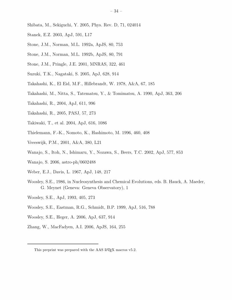
– 34 –

Shibata, M., Sekiguchi, Y. 2005, Phys. Rev. D, 71, 024014

Stanek, E.Z. 2003, ApJ, 591, L17

Stone, J.M., Norman, M.L. 1992a, ApJS, 80, 753

Stone, J.M., Norman, M.L. 1992b, ApJS, 80, 791

Stone, J.M., Pringle, J.E. 2001, MNRAS, 322, 461

Suzuki, T.K., Nagataki, S. 2005, ApJ, 628, 914

Takahashi, K., El Eid, M.F., Hillebrandt, W. 1978, A&A, 67, 185

Takahashi, M., Nitta, S., Tatematsu, Y., & Tomimatsu, A. 1990, ApJ, 363, 206

Takahashi, R., 2004, ApJ, 611, 996

Takahashi, R., 2005, PASJ, 57, 273

Takiwaki, T., et al. 2004, ApJ, 616, 1086

Thielemann, F.-K., Nomoto, K., Hashimoto, M. 1996, 460, 408

Vreeswijk, P.M., 2001, A&A, 380, L21

Wanajo, S., Itoh, N., Ishimaru, Y., Nozawa, S., Beers, T.C. 2002, ApJ, 577, 853

Wanajo, S. 2006, astro-ph/0602488

Weber, E.J., Davis, L. 1967, ApJ, 148, 217

Woosley, S.E., 1986, in Nucleosynthesis and Chemical Evolutions, eds. B. Hauck, A. Maeder,

G. Meynet (Geneva: Geneva Observatory), 1

Woosley, S.E., ApJ, 1993, 405, 273

Woosley, S.E., Eastman, R.G., Schmidt, B.P. 1999, ApJ, 516, 788

Woosley, S.E., Heger, A. 2006, ApJ, 637, 914

Zhang, W., MacFadyen, A.I. 2006, ApJS, 164, 255

This preprint was prepared with the AAS LATEX macros v5.2.

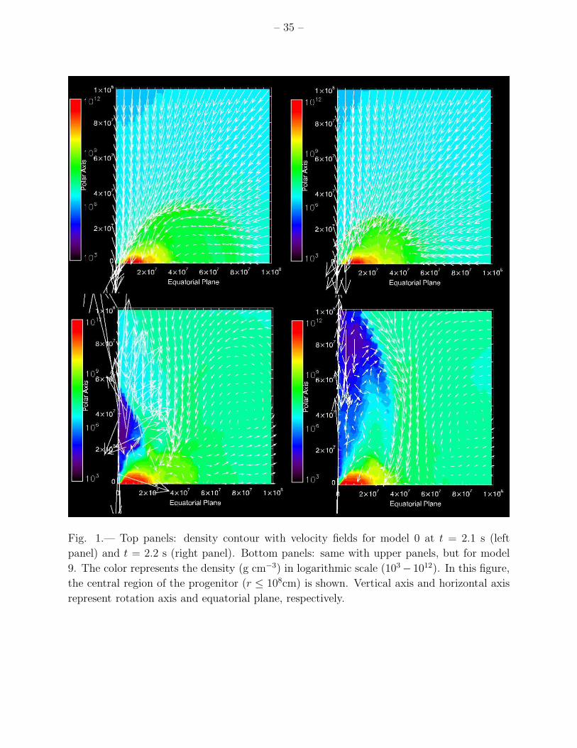
– 35 –

Fig. 1.— Top panels: density contour with velocity fields for model 0 at t = 2.1 s (left

panel) and t = 2.2 s (right panel). Bottom panels: same with upper panels, but for model

9. The color represents the density (g cm−3) in logarithmic scale (103 − 1012). In this figure,

the central region of the progenitor (r ≤ 108cm) is shown. Vertical axis and horizontal axis

represent rotation axis and equatorial plane, respectively.

– 36 –

Fig. 2.— Solid, short-dashed, dotted, dot-dashed lines represent accreted total energy, kinetic

energy, thermal energy, and electro-magnetic energy (×1050 erg) into the black hole as a

function of time, respectively. Long-dashed lines represent the mass accretion rate (M s−1)

as a function of time. Left panel shows the case for model 0, while right panel represents

the case for model 9. Note that in the case of model 0, the electro-magnetic energy is set to

be zero.

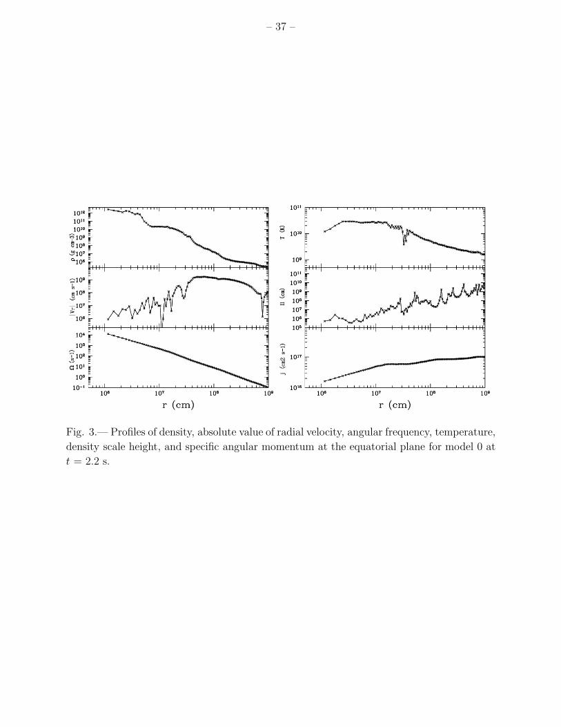
– 37 –

Fig. 3.— Profiles of density, absolute value of radial velocity, angular frequency, temperature,

density scale height, and specific angular momentum at the equatorial plane for model 0 at

t = 2.2 s.

– 38 –

Fig. 4.— Profiles of mass fraction for nuclear elements at the equatorial plane for model 0

at t = 2.2 s. Dot-dashed, dotted, short-dashed, long-dashed, and solid lines represent mass

fraction of n, p, 4He, 16O, and 56Ni, respectively.

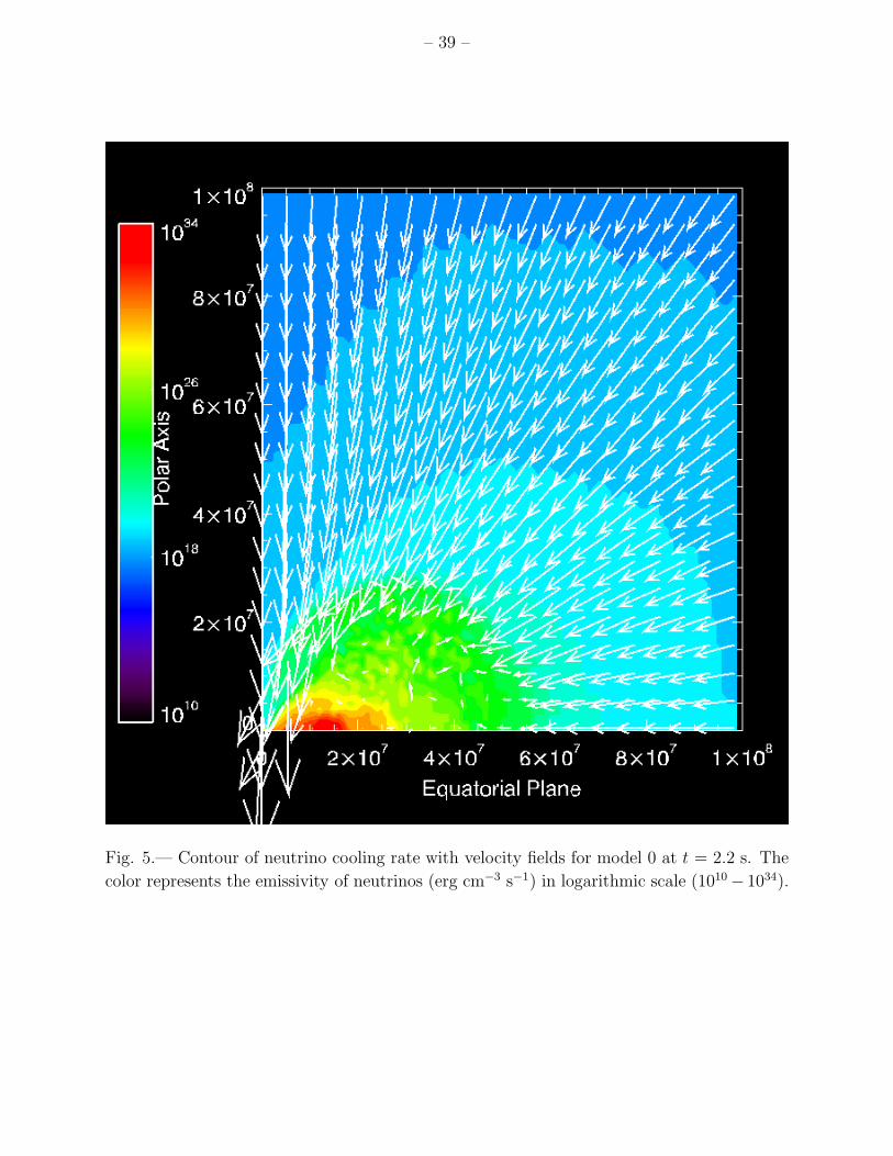
– 39 –

Fig. 5.— Contour of neutrino cooling rate with velocity fields for model 0 at t = 2.2 s. The

color represents the emissivity of neutrinos (erg cm−3 s−1) in logarithmic scale (1010 − 1034).

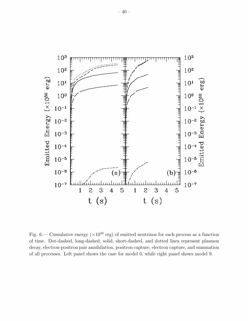
– 40 –

Fig. 6.— Cumulative energy (×1050 erg) of emitted neutrinos for each process as a function

of time. Dot-dashed, long-dashed, solid, short-dashed, and dotted lines represent plasmon

decay, electron-positron pair annihilation, positron capture, electron capture, and summation

of all processes. Left panel shows the case for model 0, while right panel shows model 9.

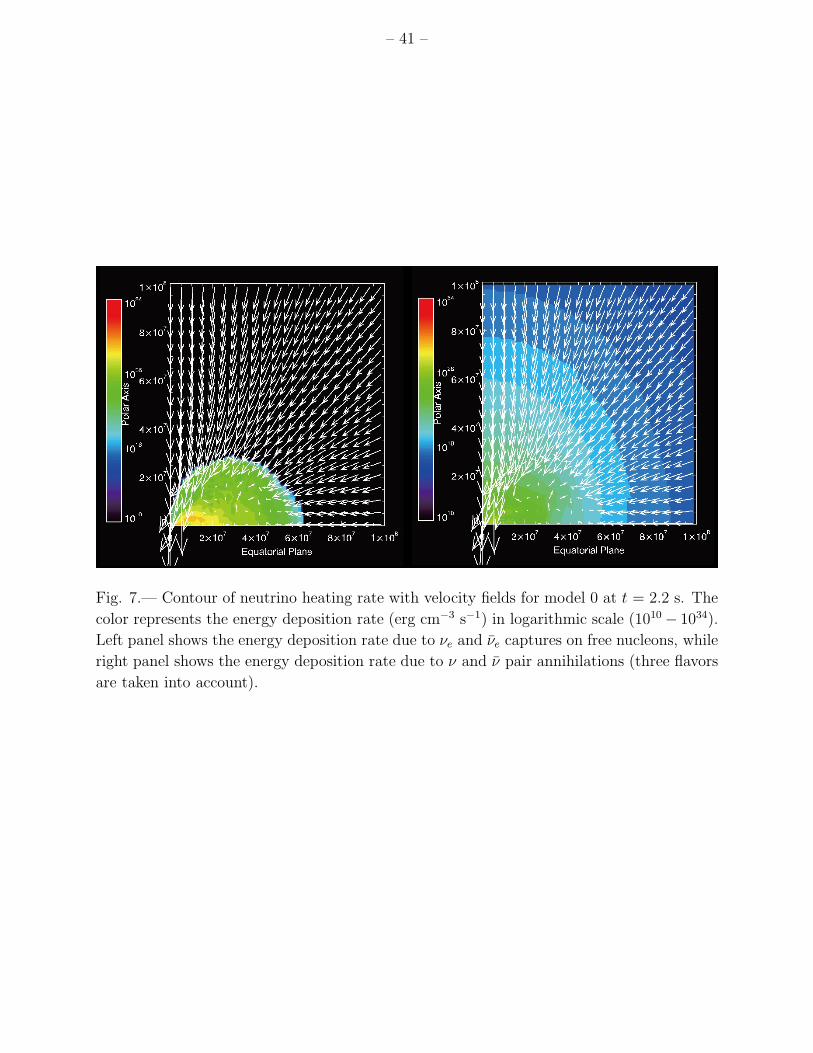
– 41 –

Fig. 7.— Contour of neutrino heating rate with velocity fields for model 0 at t = 2.2 s. The

color represents the energy deposition rate (erg cm−3 s−1) in logarithmic scale (1010 − 1034).

Left panel shows the energy deposition rate due to νe and νe captures on free nucleons, while

right panel shows the energy deposition rate due to ν and ν pair annihilations (three flavors

are taken into account).

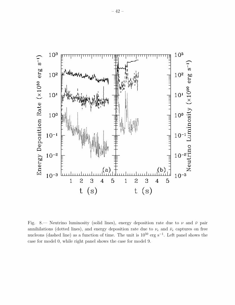
– 42 –

Fig. 8.— Neutrino luminosity (solid lines), energy deposition rate due to ν and ν pair

annihilations (dotted lines), and energy deposition rate due to νe and νe captures on free

nucleons (dashed line) as a function of time. The unit is 1050 erg s−1. Left panel shows the

case for model 0, while right panel shows the case for model 9.

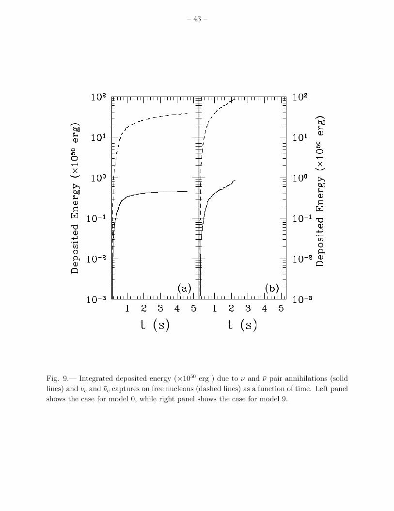
– 43 –

Fig. 9.— Integrated deposited energy (×1050 erg ) due to ν and ν pair annihilations (solid

lines) and νe and νe captures on free nucleons (dashed lines) as a function of time. Left panel

shows the case for model 0, while right panel shows the case for model 9.

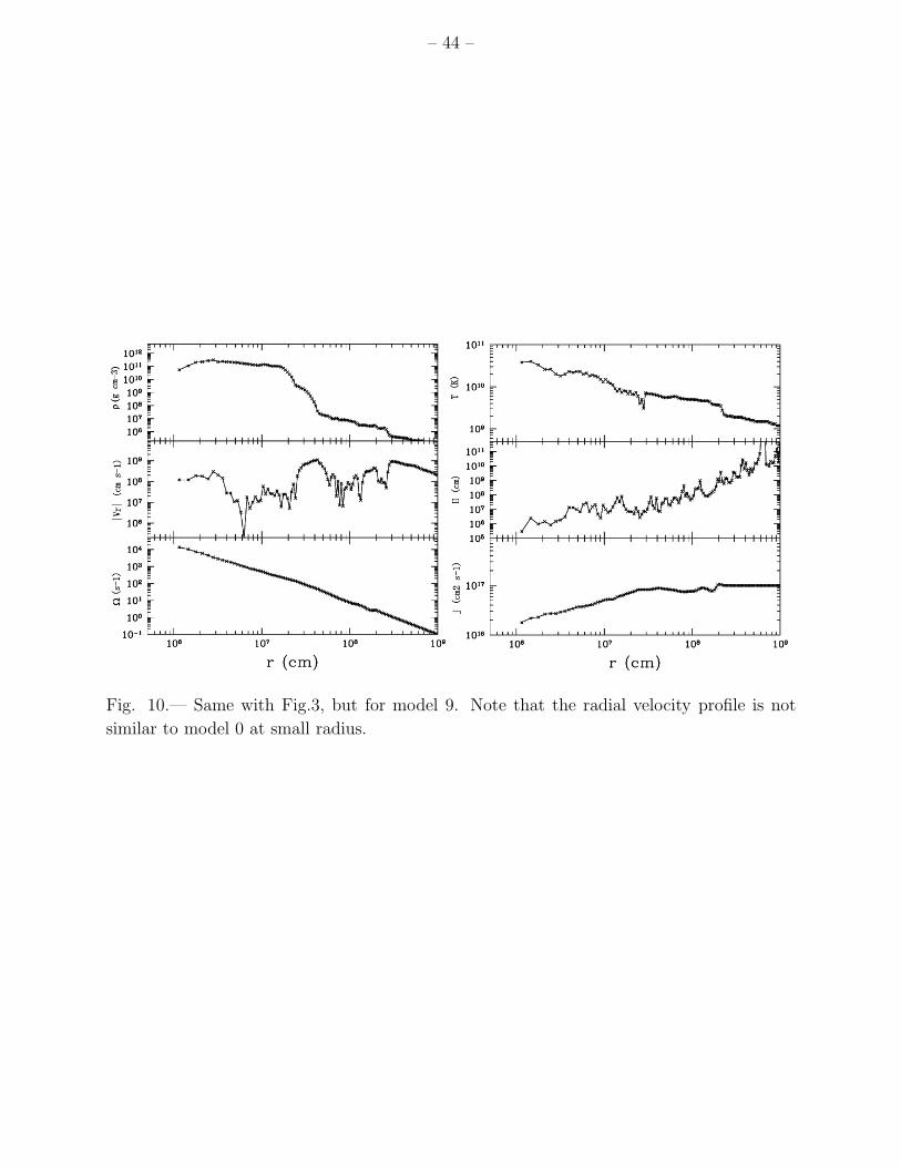
– 44 –

Fig. 10.— Same with Fig.3, but for model 9. Note that the radial velocity profile is not

similar to model 0 at small radius.

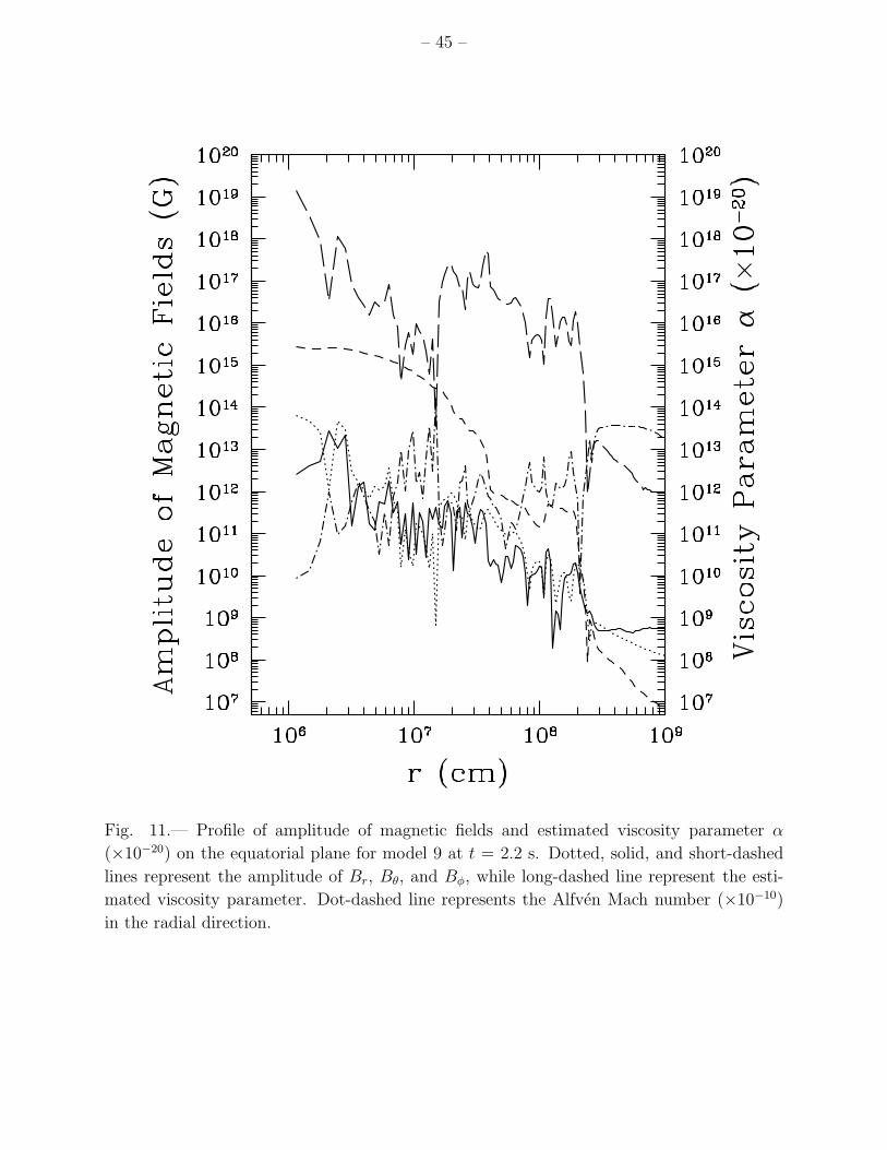
– 45 –

Fig. 11.— Profile of amplitude of magnetic fields and estimated viscosity parameter α

(×10−20) on the equatorial plane for model 9 at t = 2.2 s. Dotted, solid, and short-dashed

lines represent the amplitude of Br, Bθ, and Bφ, while long-dashed line represent the esti-

mated viscosity parameter. Dot-dashed line represents the Alfven Mach number (×10−10)

in the radial direction.

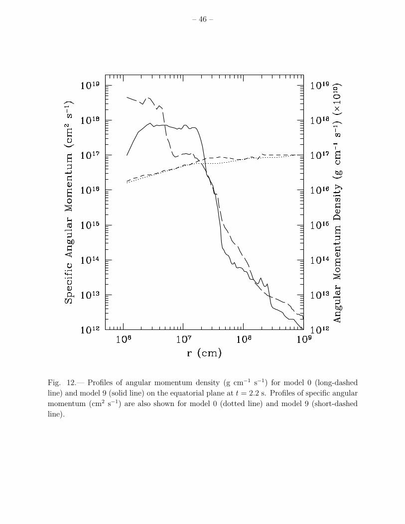
– 46 –

Fig. 12.— Profiles of angular momentum density (g cm−1 s−1) for model 0 (long-dashed

line) and model 9 (solid line) on the equatorial plane at t = 2.2 s. Profiles of specific angular

momentum (cm2 s−1) are also shown for model 0 (dotted line) and model 9 (short-dashed

line).

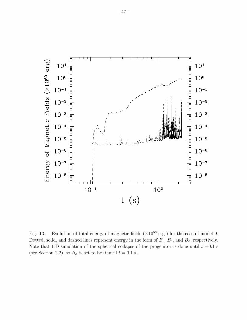
– 47 –

Fig. 13.— Evolution of total energy of magnetic fields (×1050 erg ) for the case of model 9.

Dotted, solid, and dashed lines represent energy in the form of Br, Bθ, and Bφ, respectively.

Note that 1-D simulation of the spherical collapse of the progenitor is done until t =0.1 s

(see Section 2.2), so Bφ is set to be 0 until t = 0.1 s.

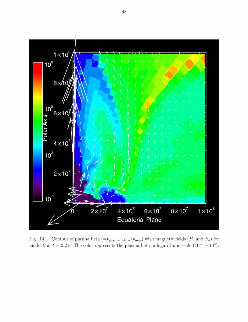
– 48 –

Fig. 14.— Contour of plasma beta (=pgas+radiation/pmag) with magnetic fields (Br and Bθ) for

model 9 at t = 2.2 s. The color represents the plasma beta in logarithmic scale (10−1 −108).

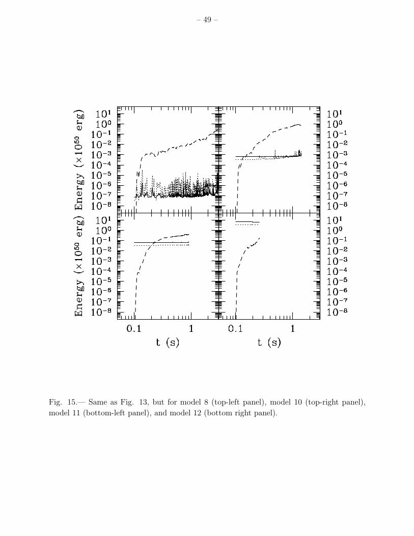
– 49 –

Fig. 15.— Same as Fig. 13, but for model 8 (top-left panel), model 10 (top-right panel),

model 11 (bottom-left panel), and model 12 (bottom right panel).

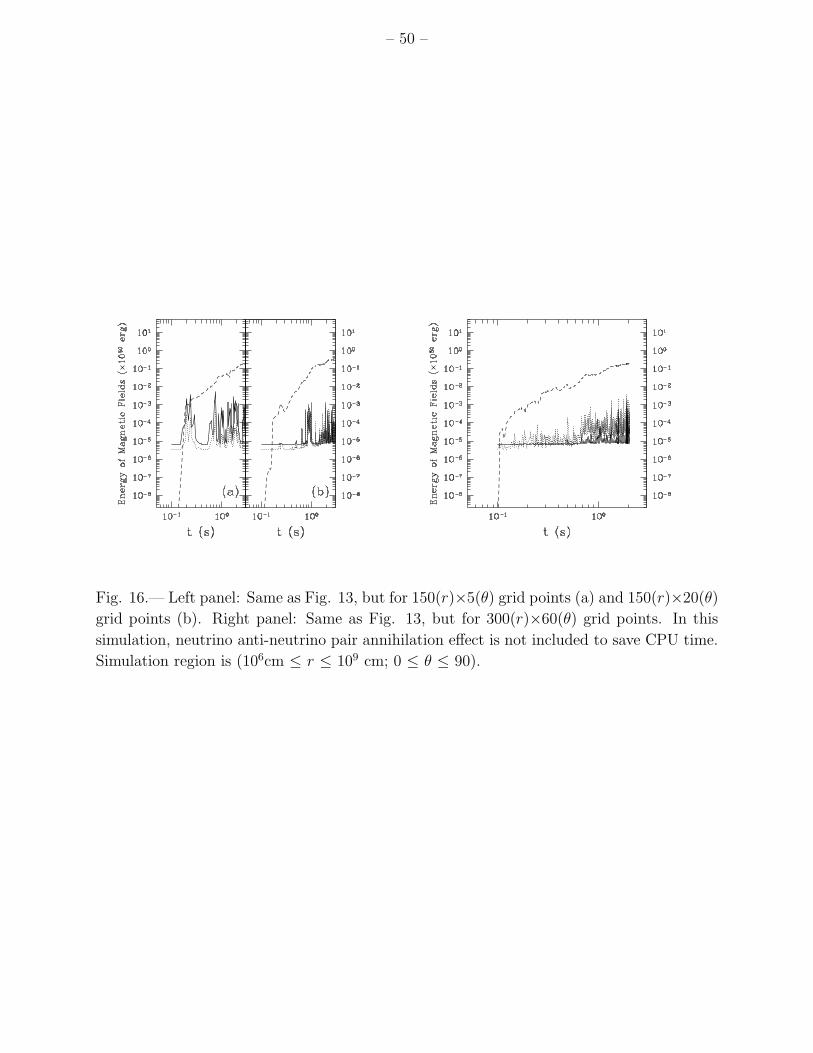
– 50 –

Fig. 16.— Left panel: Same as Fig. 13, but for 150(r)×5(θ) grid points (a) and 150(r)×20(θ)

grid points (b). Right panel: Same as Fig. 13, but for 300(r)×60(θ) grid points. In this

simulation, neutrino anti-neutrino pair annihilation effect is not included to save CPU time.

Simulation region is (106cm ≤ r ≤ 109 cm; 0 ≤ θ ≤ 90).

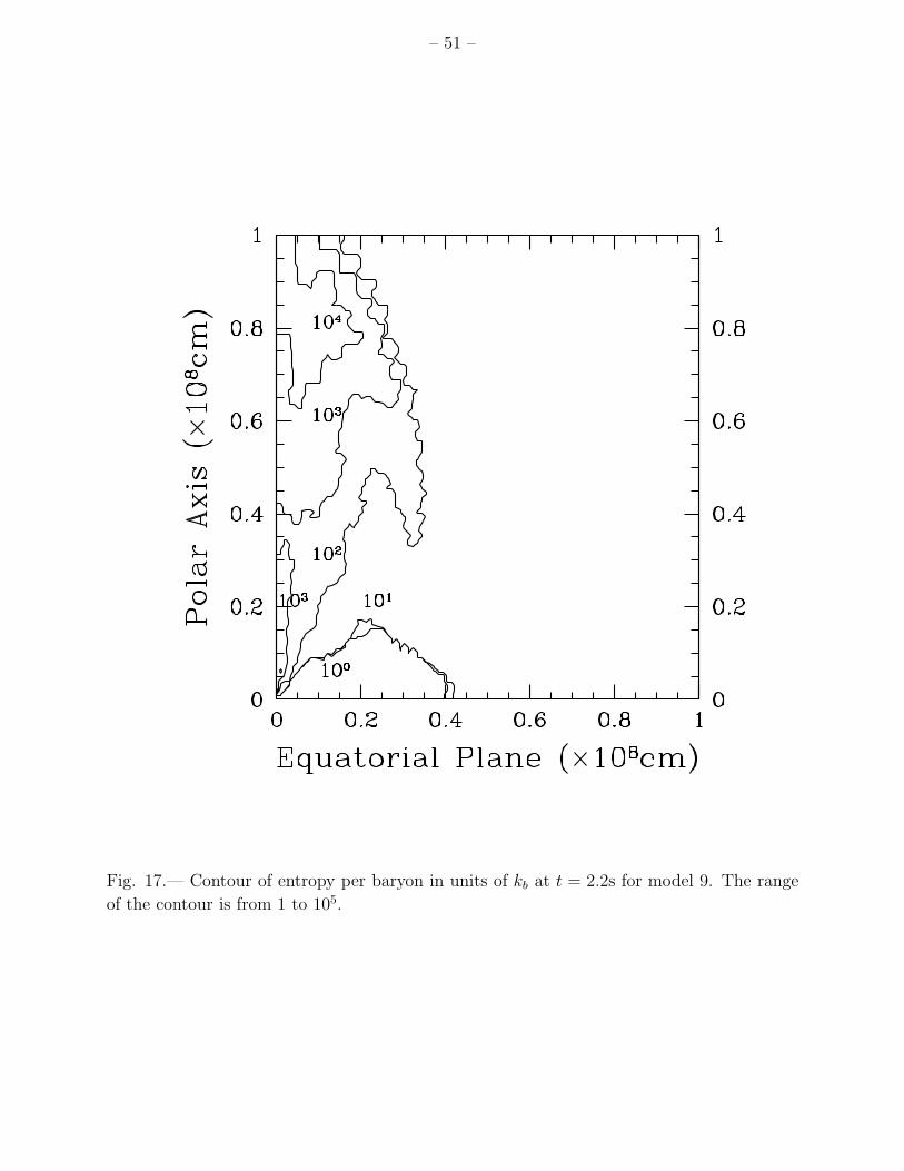
– 51 –

Fig. 17.— Contour of entropy per baryon in units of kb at t = 2.2s for model 9. The range

of the contour is from 1 to 105.

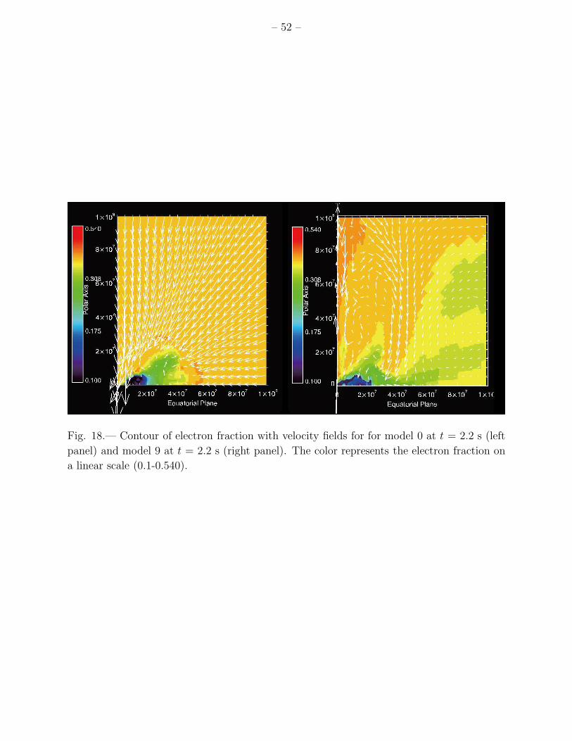
– 52 –

Fig. 18.— Contour of electron fraction with velocity fields for for model 0 at t = 2.2 s (left

panel) and model 9 at t = 2.2 s (right panel). The color represents the electron fraction on

a linear scale (0.1-0.540).

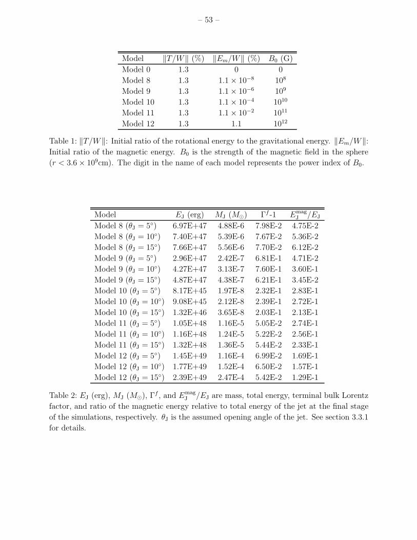
– 53 –

Model ‖T/W‖ (%) ‖Em/W‖ (%) B0 (G)

Model 0 1.3 0 0

Model 8 1.3 1.1 × 10−8 108

Model 9 1.3 1.1 × 10−6 109

Model 10 1.3 1.1 × 10−4 1010

Model 11 1.3 1.1 × 10−2 1011

Model 12 1.3 1.1 1012

Table 1: ‖T/W‖: Initial ratio of the rotational energy to the gravitational energy. ‖Em/W‖:Initial ratio of the magnetic energy. B0 is the strength of the magnetic field in the sphere

(r < 3.6 × 109cm). The digit in the name of each model represents the power index of B0.

Model EJ (erg) MJ (M) Γf -1 EmagJ /EJ

Model 8 (θJ = 5) 6.97E+47 4.88E-6 7.98E-2 4.75E-2

Model 8 (θJ = 10) 7.40E+47 5.39E-6 7.67E-2 5.36E-2

Model 8 (θJ = 15) 7.66E+47 5.56E-6 7.70E-2 6.12E-2

Model 9 (θJ = 5) 2.96E+47 2.42E-7 6.81E-1 4.71E-2

Model 9 (θJ = 10) 4.27E+47 3.13E-7 7.60E-1 3.60E-1

Model 9 (θJ = 15) 4.87E+47 4.38E-7 6.21E-1 3.45E-2

Model 10 (θJ = 5) 8.17E+45 1.97E-8 2.32E-1 2.83E-1

Model 10 (θJ = 10) 9.08E+45 2.12E-8 2.39E-1 2.72E-1

Model 10 (θJ = 15) 1.32E+46 3.65E-8 2.03E-1 2.13E-1

Model 11 (θJ = 5) 1.05E+48 1.16E-5 5.05E-2 2.74E-1

Model 11 (θJ = 10) 1.16E+48 1.24E-5 5.22E-2 2.56E-1

Model 11 (θJ = 15) 1.32E+48 1.36E-5 5.44E-2 2.33E-1

Model 12 (θJ = 5) 1.45E+49 1.16E-4 6.99E-2 1.69E-1

Model 12 (θJ = 10) 1.77E+49 1.52E-4 6.50E-2 1.57E-1

Model 12 (θJ = 15) 2.39E+49 2.47E-4 5.42E-2 1.29E-1

Table 2: EJ (erg), MJ (M), Γf , and EmagJ /EJ are mass, total energy, terminal bulk Lorentz

factor, and ratio of the magnetic energy relative to total energy of the jet at the final stage

of the simulations, respectively. θJ is the assumed opening angle of the jet. See section 3.3.1

for details.

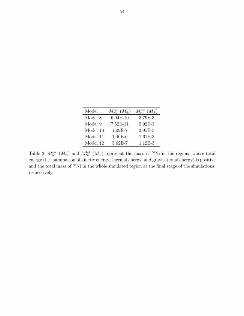
– 54 –

Model M escNi (M) M tot

Ni (M)

Model 8 6.04E-10 3.79E-3

Model 9 7.52E-11 5.92E-3

Model 10 1.09E-7 3.95E-3

Model 11 1.40E-6 1.61E-3

Model 12 5.62E-7 1.12E-3

Table 3: M escNi (M) and M tot

Ni (M) represent the mass of 56Ni in the regions where total

energy (i.e. summation of kinetic energy, thermal energy, and gravitational energy) is positive

and the total mass of 56Ni in the whole simulated region at the final stage of the simulations,

respectively.