1 © 2015 IOP Publishing Ltd Printed in the UK

1. Introduction

The Korringa–Kohn–Rostoker Green function method (KKR)in the framework of density functional theory [1] has been a powerful tool for electronic structure calculations in the past decades. Although it is based on the early work of Korringa [2] and Kohn and Rostoker [3] in 1947 and 1954, respectively, an active development of the method is present also today [4]. Originally, the KKR method was formulated for non-relativ-istic approximations using muffin-tin spheres for the descrip-tion of the potentials. Significant extensions of the original method are given by the relativistic KKR method [5, 6], by the full-potential KKR method [7, 8] and by the combination of both, the fully-relativistic full-potential KKR method [9]. These developments allow for precise calculations of total energies and forces including relativistic effects. This opens new perspectives for many applications [4] such as structure optimisations, equations of states and phonons.

The KKR method is based on the multiple scattering theory, whereas a periodic system is separated into disjoint atomic regions which represent scattering centres. Since the Green function is constructed from the regular and irregular single-site scattering solutions at each lattice site, an accurate numerical solution of the underlying differential equations is crucial. Within the non-relativistic full-potential KKR method, it was suggested by Drittler [7], to solve the underlying single-site scattering problem by means of a Lippmann–Schwingerequation, i.e. in terms of integral equations. In general, these integral equations can be solved iteratively via Born series. Later it was suggested to reformulate the original approach by means of integral equations of Volterra type to achieve better convergence properties [10, 11]. Huhne et al [9] showed that the original approach of Drittler can be used as well in the relativistic KKR method, where instead of the Schrödingerequation, the Dirac equation has to be solved. One of the dis-advantages of the original implementation is given by the fact

Journal of Physics: Condensed Matter

Numerical solution of the relativistic single-site scattering problem for the Coulomb and the Mathieu potential

Matthias Geilhufe1, Steven Achilles2, Markus Arthur Köbis3, Martin Arnold3, Ingrid Mertig1,2, Wolfram Hergert2 and Arthur Ernst1

1 Max Planck Institute of Microstructure Physics, Weinberg 2, D-06120 Halle (Saale), Germany2 Martin Luther University Halle-Wittenberg, Institute of Physics, Von-Seckendorff-Platz 1, D-06120 Halle (Saale), Germany3 Martin Luther University Halle-Wittenberg, Institute for Mathematics, Theodor-Lieser-Str. 5, D-06120 Halle (Saale), Germany

E-mail: geilhufe@mpi-halle.de

Received 26 June 2015, revised 17 August 2015Accepted for publication 1 September 2015Published 8 October 2015

AbstractFor a reliable fully-relativistic Korringa–Kohn–Rostoker Green function method, an accuratesolution of the underlying single-site scattering problem is necessary. We present an extensive discussion on numerical solutions of the related differential equations by means of standard methods for a direct solution and by means of integral equations. Our implementation is tested and exemplarily demonstrated for a spherically symmetric treatment of a Coulomb potential and for a Mathieu potential to cover the full-potential implementation. For the Coulomb potential we include an analytic discussion of the asymptotic behaviour of irregular scattering solutions close to the origin ( r 1).

Keywords: Korringa–Kohn–Rostoker Green function method, irregular solution, full-potential,relativistic, Mathieu potential, Coulomb potential, single-site scattering

(Some figures may appear in colour only in the online journal)

M Geilhufe et al

Numerical solution of the relativistic single-site scattering problem for the Coulomb and the Mathieu potential

Printed in the UK

435202

JCOMEL

© 2015 IOP Publishing Ltd

2015

27

J. Phys.: Condens. Matter

CM

0953-8984

10.1088/0953-8984/27/43/435202

Papers

43

Journal of Physics: Condensed Matter

IOP

0953-8984/15/435202+10$33.00

doi:10.1088/0953-8984/27/43/435202J. Phys.: Condens. Matter 27 (2015) 435202 (10pp)

TH-2015-38

M Geilhufe et al

2

that a certain cut-off radius R0 close to the origin has to be introduced in order to avoid problems arising from the treat-ment of the irregular single-site scattering solutions. Recently, it was shown by Zeller [12], that this approximation might be inconvenient for materials like NiTi and that the cut-off radius can be chosen arbitrarily small by using an analytical decou-pling scheme and a subinterval procedure with Chebyshev interpolations in each subinterval.

In the present paper we follow a different approach and discuss besides the solution via integral equations, the direct solution of the fully relativistic full-potential single-site scat-tering problem by means of standard methods for ordinary differential equations. We demonstrate that both the regular as well as the irregular scattering solutions can be obtained with high accuracy. To demonstrate this, we first discuss the solution of the spherical Coulomb potential. Furthermore, we derive the asymptotic behaviour of the relativistic irregular scattering solutions and show that within the limit towards a non-relativistic description their asymptotic behaviour dif-fers significantly from the non-relativistic irregular scattering solutions. Second, we discuss the solution of the fully relativ-istic full-potential single-site scattering problem for a Mathieu potential in simple cubic lattice and compare different applied solvers. The Mathieu potential is highly anisotropic and thus, it is an ideal test system. Moreover, this potential is not of purely academic type since it can be seen as an approxima-tion to the potential in empty spheres that have to be included in the description of non-close-packed structures, e.g. for semiconductors or oxides [13–15]. Additionally, the Mathieu potential allows to evaluate all quantities analytically and is therefore ideal for a comparison with numerical results. For illustrative purposes we show the bandstructure represented by the Bloch spectral function.

2. Single-site scattering

In this section we focus on the Dirac or Kohn–Sham–Dirac

equation [16, 17] in atomic Rydberg units ( = 1, =m 1

2,

= ≈α

c 2742 ) applied to non-magnetic systems,

⎡⎣⎢

⎤⎦⎥c c I V r r W ri

1

2,2

4 eff→ ( ) ( ) ( )

→ → → → → →α β φ φ− = ⋅ ∇ +=

+ = =Λ Λ (1)

where the index Λ denotes a combined index ( )κ µ, . According to Huhne et al [9] the equation above can be solved via expanding the solution ( )φΛ

→ →r , which is a four component spinor-function, into so called spin-angular functions ( ˆ)χΛ′

→ r ,

∑φχχ

=ΛΛ

ΛΛ Λ

ΛΛ Λ′

′ ′

′ ′

⎛

⎝⎜

⎞

⎠⎟r

g r r

f r ri.( )

( ) ( ˆ)( ) ( ˆ)

→ →→

→ (2)

The spin-angular functions, ( ˆ) ( ˆ)χ ξ= ∑ µΛ Λ

−→ →r C Y rm

ml

mms

s ss,

are given by a linear combination of complex spherical har-

monics ( ˆ)Y rlm and the Pauli spinors ξ

→

ms, whereas the expan-

sion coefficients ΛCms denote the Clebsch–Gordan coefficients

( )( )µ−C l j m m, s s1

2 [18]. Using the orthogonality of the

spin-angular functions and by defining the matrix V r( )= with

components χ χ=ΛΛ Λ Λ′ ′→ →V Veff the following system of

coupled first-order ordinary differential equations can be obtained:

⎛⎝⎜

⎞⎠⎟c

r r rf

cg V g Wg

1

2,

2

∑κ−

∂∂

+ − + + =′

″″ ″ΛΛ ΛΛ

ΛΛΛ Λ Λ ΛΛ′ ′ ′ ′

(3)

∑κ∂

∂+ + − + =

′

″″ ″ΛΛ ΛΛ

ΛΛ Λ Λ Λ ΛΛ′ ′ ′ ′⎜ ⎟

⎛⎝

⎞⎠c

r r rg

cf V f Wf

1

2.

2

(4)

By definition, the potential ( )→V reff is constructed such that it is non-zero within the Wigner–Seitz cell of a certain atomic site and zero outside. To obtain this behaviour ( )→V reff is given as the product of a non-spherical potential ( )→U reff and the shape-truncation function ( )Θ →r [19, 20],

( ) ( ) ( )= Θ→ → →V r U r r .eff eff (5)

The elements of the potential matrix of the effective potential ( )→V reff , based on an expansion in terms of complex spherical

harmonics, are given by

( ) ( ) ( ) ( )∑ ∑=″ ″

″ ″ ″″µ µ

ΛΛ Λ Λ− −

′ ′ ′′V r C C V r G .

l m m

m ml m l l l

m m m,

s

s s s s

(6)

For the construction of the Green function, it is necessary to obtain two linearly independent solutions ( )φΛ

→ →r . First, a solution ( )Λ

→ →R r , which is regular at the origin, and second, a solution ( )Λ

→ →H r , which is singular at the origin. Outside of the Wigner–Seitz cell both solutions can be constructed from the spherical Bessel functions jl(r) and the spherical Hankel functions ( ) ( ) ( )= +h r j r in rl l l , which are a linear combina-tion of the spherical Bessel and the spherical Neumann func-tions nl(r). By introducing the single-site scattering t-matrix

=t , the regular single-site scattering solution outside of the Wigner–Seitz cell can be written in the following way [8, 9],

⎡

⎣⎢⎢

⎛

⎝⎜⎜

⎞

⎠⎟⎟

⎛

⎝⎜⎜

⎞

⎠⎟⎟

⎤

⎦⎥⎥R r

j kr r

e j kr rk

h kr r

e h kr rti ,l

l

l

l

outside( )

( ) ( ˆ)

( ) ( ˆ)

( ) ( ˆ)

( ) ( ˆ)→ →

→ →

→ →

→ →

→ →∑χ

χδ

χ

χ= −Λ

Λ

Λ

Λ ΛΛΛ

Λ

Λ ΛΛΛ

′

′ ′

′ ′ ′′

′ ′

′ ′ ′′

(7)

by using the abbreviations ( )κ=Λ +e signck

E c

i2 , ( )κ= −l l sign ,

and the relativistic momentum ( )ε= + εk 1c2 with . ε =

W − c2 The associated irregular single-site scattering solution is given by

( )( ) ( ˆ)( ) ( ˆ)χ

χ=Λ

Λ

Λ Λ

→ →→ →

→ →

⎛

⎝⎜⎜

⎞

⎠⎟⎟H r

h kr r

e h kr r.

l

l

outside (8)

In the following we will discuss two different approaches for the numerical solution of equations (3) and (4) inside the Wigner–Seitz cell.

2.1. Numerical solution of the differential equations

For a numerical treatment of equations (3) and (4) it is common to transform the large and the small component of the solution according to

J. Phys.: Condens. Matter 27 (2015) 435202

M Geilhufe et al

3

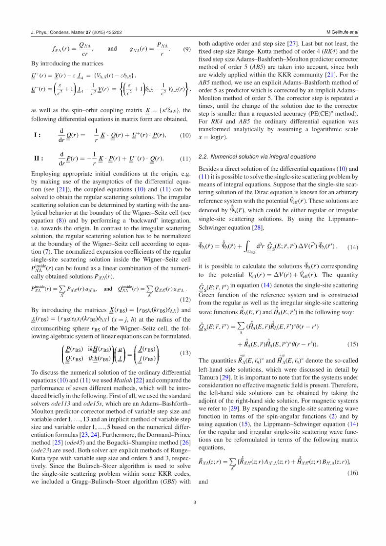
( ) ( )= =ΛΛΛΛ

ΛΛΛΛ

′′

′′f r

Q

crg r

P

r, and . (9)

By introducing the matrices

⎜ ⎟ ⎜ ⎟⎛⎝

⎞⎠

⎧⎨⎩

⎛⎝

⎞⎠

⎫⎬⎭

U r V r I V r

U rc

Ic

V rc c

V r

,

11

11

,

4 ,

2 4 2 2 2 ,

( ) ( ) ( )

( ) ( ) ( )

ε εδ

ε εδ

= = = − = = −

= = + = − = = + −

+Λ Λ ΛΛ

−ΛΛ Λ Λ

′ ′

′ ′

as well as the spin–orbit coupling matrix κ δ= = ′ ΛΛ′K , the following differential equations in matrix form are obtained,

( ) ( ) ( ) ( )=

= = ⋅=

+ = ⋅ =+

rQ r

rK Q r U r P rI :

d

d

1, (10)

rP r

rK P r U r Q rII :

d

d

1.( ) ( ) ( ) ( )= = − = ⋅ = + = ⋅

=− (11)

Employing appropriate initial conditions at the origin, e.g. by making use of the asymptotics of the differential equa-tion (see [21]), the coupled equations (10) and (11) can be solved to obtain the regular scattering solutions. The irregular scattering solution can be determined by starting with the ana-lytical behavior at the boundary of the Wigner–Seitz cell (see equation (8)) and by performing a ‘backward’ integration, i.e. towards the origin. In contrast to the irregular scattering solution, the regular scattering solution has to be normalized at the boundary of the Wigner–Seitz cell according to equa-tion (7). The normalized expansion coefficients of the regular single-site scattering solution inside the Wigner–Seitz cell

( )ΛΛ′P rinside can be found as a linear combination of the numeri-cally obtained solutions ( )ΛΛ′P r ,

( ) ( ) ( ) ( ) ∑ ∑= =″

″ ″″

″ ″ΛΛΛ

ΛΛ Λ Λ ΛΛΛ

ΛΛ Λ Λ′ ′ ′ ′P r P r a Q r Q r a, and .inside inside

(12)

By introducing the matrices ( ) ( ) δ= = ΛΛ′X r r x krlBS BS BS and ( ) ( ) δ= = Λ ΛΛ′x r r ce x krlBS BS BS (x = j, h) at the radius of the

circumscribing sphere rBS of the Wigner–Seitz cell, the fol-lowing algebraic system of linear equations can be formulated,

⎛

⎝⎜⎜

⎞

⎠⎟⎟⎛⎝⎜

⎞⎠⎟

⎛

⎝⎜⎜

⎞

⎠⎟⎟

P r kH r

Q r k h r

at

J r

j r

i

i.

BS BS

BS BS

BS

BS

( ) ( )( ) ( )

( )( )

= =

= ===

= =

= (13)

To discuss the numerical solution of the ordinary differential equations (10) and (11) we used Matlab [22] and compared the performance of seven different methods, which will be intro-duced briefly in the following. First of all, we used the standard solvers ode113 and ode15s, which are an Adams–Bashforth–Moulton predictor-corrector method of variable step size and variable order …1, , 13 and an implicit method of variable step size and variable order …1, , 5 based on the numerical differ-entiation formulas [23, 24]. Furthermore, the Dormand–Prince method [25] (ode45) and the Bogacki–Shampine method [26] (ode23) are used. Both solver are explicit methods of Runge–Kutta type with variable step size and orders 5 and 3, respec-tively. Since the Bulirsch–Stoer algorithm is used to solve the single-site scattering problem within some KKR codes, we included a Gragg–Bulirsch–Stoer algorithm (GBS) with

both adaptive order and step size [27]. Last but not least, the fixed step size Runge–Kutta method of order 4 (RK4) and the fixed step size Adams–Bashforth–Moulton predictor corrector method of order 5 (AB5) are taken into account, since both are widely applied within the KKR community [21]. For the AB5 method, we use an explicit Adams–Bashforth method of order 5 as predictor which is corrected by an implicit Adams–Moulton method of order 5. The corrector step is repeated n times, until the change of the solution due to the corrector step is smaller than a requested accuracy (PE(CE)n method). For RK4 and AB5 the ordinary differential equation was transformed analytically by assuming a logarithmic scale

( )=x rlog .

2.2. Numerical solution via integral equations

Besides a direct solution of the differential equations (10) and (11) it is possible to solve the single-site scattering problem by means of integral equations. Suppose that the single-site scat-tering solution of the Dirac equation is known for an arbitrary reference system with the potential ( )→V reff . These solutions are

denoted by ( )ΨΛ→ →r˚ , which could be either regular or irregular

single-site scattering solutions. By using the Lippmann–Schwinger equation [28],

r r r G E r r V r r˚ d ˚ ; , ,3S

WS

( ) ( ) ( ) ( ) ( ) → → → → → → → → →∫Φ = Ψ + = ∆ Φ′ ′ ′Λ Λ

ΩΛ (14)

it is possible to calculate the solutions ( )ΦΛ→ →r corresponding

to the potential ( ) ( ) ( )= ∆ +→ → →V r V r V r˚eff eff . The quantity

G E r r˚ ; ,S( )→ →

= ′ in equation (14) denotes the single-site scattering

Green function of the reference system and is constructed from the regular as well as the irregular single-site scattering

wave functions ( )Λ→ →R E r˚ , and ( )′Λ

→ →H E r˚ , in the following way:

( ) ( ( ) ( ) ( )

( ) ( ) ( ))

→ → → → → →

→ → → →

∑ θ

θ

= = −

+ −

′ ′ ′

′ ′

ΛΛ Λ

×

Λ Λ×

G E r r H E r R E r r r

R E r H E r r r

˚ ; , ˚ , ˚ ,

˚ , ˚ , .

S

(15)

The quantities ( )Λ×→ →R E r˚ ,

n

n and ( )Λ×→ →H E r˚ ,

n

n denote the so-called

left-hand side solutions, which were discussed in detail by Tamura [29]. It is important to note that for the systems under consideration no effective magnetic field is present. Therefore, the left-hand side solutions can be obtained by taking the adjoint of the right-hand side solution. For magnetic systems we refer to [29]. By expanding the single-site scattering wave function in terms of the spin-angular functions (2) and by using equation (15), the Lippmann–Schwinger equation (14) for the regular and irregular single-site scattering wave func-tions can be reformulated in terms of the following matrix equations,

( ) [ ( ) ( ) ( ) ( )]→ → →

∑= +″

″ ″ ″ ″ΛΛΛ

ΛΛ Λ Λ ΛΛ Λ Λ′ ′ ′R z r R z r A z r H z r B z r; ˚ ; ; ˚ ; ; ,, ,

(16)and

J. Phys.: Condens. Matter 27 (2015) 435202

M Geilhufe et al

4

( ) [ ( ) ( ) ( ) ( )]∑= +″

″ ″ ″ ″ΛΛΛ

ΛΛ Λ Λ ΛΛ Λ Λ′ ′ ′→ → →H z r R z r C z r H z r D z r; ˚ ; ; ˚ ; ; ., ,

(17)

The matrices ( )=A z r, , B z r,( )= , C z r,( )= and D z r,( )= contain the integrals over the radial amplitudes ( )ΛΛ′g rR H, and ( )ΛΛ′f rR H, as well as the functions ( )ΛΛ′x rR H, and ( )ΛΛ′y rR H, , which include the solutions of the reference system and the change of the potential ( )∆ →V r ,

( )

( ( ) ( )

( ) ( ))

∫∑

δ=

+

+

′ ′ ′ ′

′ ′

Λ Λ Λ Λ

ΛΛ Λ Λ Λ

Λ Λ Λ Λ

′ ′

′

′

A z r

r r x z r g z r

y z r f z r

;

d ; ;

; ; ,

r

RH R

H R

, ,

2, ,

, ,

2

BS

2 2

2 2

(18)

( ) ( ( ) ( )

( ) ( ))

∫ ′∑=

+

′ ′ ′

′ ′

Λ ΛΛ

Λ Λ Λ Λ

Λ Λ Λ Λ

′ ′

′

B z r r r x z r g z r

y z r f z r

; d ; ;

; ; ,

rR R

R R

, 02

, ,

, ,

22 2

2 2

(19)

C z r r r x z r g z r

y z r f z r

; d ; ;

; ; ,

r

RH H

H H

,2

, ,

, ,

2

BS

2 2

2 2

( ) ( ( ) ( )

( ) ( ))

∫ ′∑=

+

′ ′ ′

′ ′

Λ ΛΛ

Λ Λ Λ Λ

Λ Λ Λ Λ

′ ′

′

(20)

( ) ( ( ) ( )

( ) ( ))

∫ ′∑δ= −

+

′ ′ ′

′ ′

Λ Λ Λ ΛΛ

Λ Λ Λ Λ

Λ Λ Λ Λ

′ ′ ′

′

D z r r r x z r g z r

y z r f z r

; d ; ;

; ; .

r

RR H

R H

, ,2

, ,

, ,

2

BS

2 2

2 2

(21)

The explicit expressions of ( )ΛΛ′x rR H, and ( )ΛΛ′y rR H, are given by

( ) ( ) ( ) ∑= − ∆′ ′ ′Λ ΛΛ

Λ Λ Λ Λ′ ′x z r p g z r V r; i ˚ ; ,H H, , ,2

1

1 1 2 (22)

( ) ( ) ( ) ∑= − ∆′ ′ ′Λ ΛΛ

Λ Λ Λ Λ′ ′y z r p f z r V r; i ˚ ; ,H H

, , ,2

1

1 1 2 (23)

( ) ( ) ( ) ∑= − ∆′ ′ ′Λ ΛΛ

Λ Λ Λ Λ′ ′x z r p g z r V r; i ˚ ; ,R R, , ,2

1

1 1 2 (24)

( ) ( ) ( ) ∑= − ∆′ ′ ′Λ ΛΛ

Λ Λ Λ Λ′ ′y z r p f z r V r; i ˚ ; .R R

, , ,2

1

1 1 2 (25)

In general, the Lippmann–Schwinger equation (14) is solved

iteratively in terms of Born series by starting with the reference

solution ( ) ( )( )Φ = ΨΛ Λ→ → → →r r˚0

on the right hand side of equation (14) and by calculating a better approximation ( )( )

ΦΛ→ →r

1 by integration.

This scheme is repeated, until the difference between two succes-

sive approximations, ( )( )ΦΛ→ →r

n and ( )( )

ΦΛ−→ →r

n 1, is reasonably small.

3. The Coulomb potential

3.1. Asymptotic behaviour

The Coulomb potential is spherically symmetric and hence, the expansion into spherical harmonics only consists of one (spherically symmetric) component V00(r),

( )πδ δ= −V r

Z

r

1.lm l m,0 ,0 (26)

The associated ordinary differential equations are independent of the relativistic magnetic quantum number μ and diagonal in κ, but coupled with respect to κg and κf ,

( ) ( )κ− − + − =κ κ

⎡⎣⎢

⎤⎦⎥

⎡⎣⎢

⎤⎦⎥

c Z

rW g r

c

r

c

r rr f r

2

2 d

d0

2

(27)

( ) ( )κ+ − + + =κ κ

⎡⎣⎢

⎤⎦⎥

⎡⎣⎢

⎤⎦⎥

c

r

c

r rr g r

c Z

rW f r

d

d 2

20.

2

(28)

It was pointed out by Swainson and Drake [30] that equa-tions (27) and (28) can be decoupled by transforming the radial solutions according to

( )˜ ( )˜ ( )

( )( )

= ⋅κ

κ

κ

κ

⎛

⎝⎜

⎞

⎠⎟

⎛⎝⎜

⎞⎠⎟

g r

f rX

X

g r

f r1

1. (29)

Here, the newly introduced quantities are given by ( )= γ κ−XcZ

2

and γ κ= − Z

c2 4 2

2 . By using the abbreviations =ε W

c,

( )ω = −c W

c2

2

2, and by combining equation (29) together with

(27) and (28), two differential equations of second order can be obtained, which are similar to the form of the radial Schrödinger equation,

( )˜ ( )γ γ α

ω+ −+

+ − =κε⎡

⎣⎢⎤⎦⎥r r r r

Z

rg r

d

d

2 d

d

1 20,

2

2 22 (30)

( ) ˜ ( )γ γ αω+ −

−+ − =κ

ε⎡⎣⎢

⎤⎦⎥r r r r

Z

rf r

d

d

2 d

d

1 20.

2

2 22 (31)

Close to the origin ( r 1), in the asymptotic limit, only the angular momentum terms (∼ −r 2) have to be taken into account, whereas the potential (∼ −r 1) and the constant factor ω2 can be neglected. The solution of the resulting dif-ferential equations are rational functions of the following form,

˜ = +κγ γ− −g c r c r ,1 2

1 (32)

˜ = +κγ γ− −f c r c r .3

14 (33)

Since both solutions κg and κf are linear combinations of

κg and κf , it can be verified, that the leading term for the irregular solutions is given by γ− −r 1. In the non-relativistic

limit ( ≈ 0Z

c

4 2

2 ) the asymptotic behaviour of an irregular

s-wave function (κ = −1, l = 0) close to the origin is given by

=κ− − −r r1 2 which is in contradiction to the non-relativistic solution =− − −r rl 1 1. Since the relativistic quantum number κ takes on values either κ = l or l 1κ = − − , this disagree-ment can be generalized for all irregular wave functions with

l 1κ = − − . To verify the solution behaviour for r 1, a double

logarithmic plot of the numerical solution for Z = 79 and

=α

c 2 and various values for κ is illustrated in figure 1. The

predicted asymptotic behaviour is clearly revealed.

J. Phys.: Condens. Matter 27 (2015) 435202

M Geilhufe et al

5

3.2. Numerical accuracy

For the discussion of the numerical accuracy for the solu-tion of the differential equation (equations (30) and (31)), a Coulomb potential with an atomic number of Z = 79 was used since it represents the element gold (Au). Due to the large atomic mass and non-negligible spin–orbit coupling, which causes the typical golden colour, it is a prominent example for relativistic effects. Solutions were obtained up to a maximal angular momentum quantum number of l = 5. To obtain a scattering state, the energy of the scattering solution was chosen to be ε = 1. In the following test, a spherical cell was constructed including a minimal radius of = −r 100

4 and a maximal radius of =r 3BS .

The numerical solutions obtained by using different solvers were compared with a reference solution, which was obtained by using ode113 and very high accuracy goals. For the solvers taken from the Matlab ode-suite absolute

and relative tolerances were chosen to be equal and values between 10−1 and 10−10 were used. The maximal relative error of the numerically obtained solutions as a function of the number of right-hand side evaluations of the differential equa-tion is shown in figure 2. First of all, it can be verified that the numerical accuracy of the solution of the regular single-site scattering solution (figure 3(a)) is similar to the results of the irregular single-site scattering solution (figure 3(b)), which is a first indication for non-stiff problems [31]. As pointed out by Söderlind et al [32] a rigorous mathematical definition of stiffness is difficult and a lot of controversy exists [33, 34]. Following the historical definition of stiffness [35] an ordinary differential equation is called stiff, if the numerical solution via implicit methods performs much better than the solution via explicit methods. However, for the present example it can be verified that the method ode113, which is a method for non-stiff equations, performs better than the implicit method ode15s. Since we observed poor performance for other

Figure 1. Double-logarithmic plot of the real part of relativistic irregular single-site scattering solutions for a Coulomb potential (Z = 79) close to the origin.

10−6 10−5 10−4 10−310−1

103

107

1011

1015

1019

Radius r

g κ|

κ = −1κ = 1κ = −2κ = 2κ = −3

Figure 2. Maximal relative error versus number of right-hand side (RHS) evaluations of the Dirac equation for a Coulomb potential using different methods for the solution.

102 103 104 105

10−9

10−7

10−5

10−3

10−1

101

a) Regular solution

Number of RHS evaluations

Max

imal

rela

tive

erro

r

103 104 105

b) Irregular solution

Number of RHS evaluations

ode113ode15sode45ode23RK4AB5GBS

J. Phys.: Condens. Matter 27 (2015) 435202

M Geilhufe et al

6

implicit methods, we conclude that the underlying differential equations for the Coulomb potential are non-stiff. The perfor-mance of the Dormand–Prince method (ode45) is very good for crude tolerances and becomes comparable to ode15s for fine tolerances. The Adams–Bashforth–Moulton predictor-corrector method of order 5 with fixed step size (AB5) is rather expensive for high tolerances. But, due to the higher order, the performance is better in comparison to the methods of the Runge–Kutta type ode23 and RK4, if high accuracy goals are demanded. Also in comparison to ode45, which has the same order, less evaluations of the right-hand side of the differen-tial equation for high accuracy goals are necessary; it is there-fore more efficient. The implemented Gragg–Bulirsch–Stoer method with both adaptive order and step-size (GBS) [27] is able to solve the differential equations with very high orders. But, for the accuracy goals in practice (≈10−8) it needs about five times as many evaluations of the right hand side of the differential equation in comparison to ode113.

In many implementations of the KKR method, solvers with fixed step size are used for spherically symmetric atomic potentials, whereas a logarithmic mesh of type ( )=x rlog or similar is employed [21]. The reason for this is that the wave functions are highly oscillating close to the nucleus, and are smooth for larger values of r. To verify that a logarithmic mesh is a reasonable choice, the step size for adaptive methods close the origin was investigated (see figures 3(a) and (b)). The step size during the numerical solution of the Coulomb–Dirac problem using ode113, ode15s, and ode45 is illustrated in figure 3(a) and compared with the step size of a logarithmic mesh. It can be verified that the step size used by ode45 is similar to the characteristic of a logarithmic mesh. However, the stair-case-like behaviour of ode113 and ode15s occurs due to the step-size strategy of the method itself, i.e. the change of the step-size is avoided as much as possible [23]. Analogously, it is possible to transform the differential equations (30) and (31) to a logarithmic scale ( )=x rlog and to investigate the

varying step size of the methods ode113, ode15s and ode45 for the numerical solution of the transformed equations (see figure 3(b)). It can be verified, that all three solvers adopt a constant step size close to the origin (x < −5), which again reassures the choice of a logarithmic scale for methods with fixed step size.

4. The Mathieu potential

4.1. Evaluation of the potential

A suitable test system for our full-potential implementation is given by a Mathieu potential [36],

( ) ( ( ) ( ) ( )) = − + +→V r U ax ay azcos cos cos ,0 (34)

that is periodic and represents here a simple cubic crystal structure. Moreover, it is highly anisotropic with respect to dif-ferent crystallographic directions and thus, it is ideal to serve as a test system. For our method it is necessary to express equations (34) in terms of complex spherical harmonics (see section 2). By using the exponential form of the cosine func-tion and by applying Bauer’s theorem,

( ) ( ˆ) ( ˆ) ∑ ∑π=⋅

=

∞

=−

→ → → →i j kr Y r Y ke 4 * ,k r

l m l

ll

l lm

lmi

0 (35)

we end up with the following equation,

( ) [ ] ( ) ( ˆ)→ →∑ ∑ππ

δ= − + +=

∞

=−

⎜ ⎟⎛⎝

⎞⎠V r U l l f j kr Y r4 cos

22 1 ,

l m l

l

m lm l lm

00

,0

(36)with coefficients f lm given by

⎧⎨⎪

⎩⎪f

l m

l m

l m

l mm

m

(( 1 1 11 ! !

! !

1 ! !

! !is even

0 is odd

.lm

m l2 2) ) ( ) ( )

( )( )

( )

= − + −

+ −+

− −−

(37)

Figure 3. Step size for the solution of the Coulomb–Dirac problem using adaptive methods. (a) Solution on a radial mesh. (b) Solution using a logarithmic scale.

−10 −5 0

0

0:02

0:04

0:06

0:08

0:1

x = ln(r)

Step

size

ode113ode15sode45

10−5 10−4 10−3

10−7

10−6

10−5

10−4

Radius

(a) (b)

r

Step

size

ode113ode15sode45log. mesh

J. Phys.: Condens. Matter 27 (2015) 435202

M Geilhufe et al

7

4.2. Numerical accuracy

Analogously to section 3.2, where the numerical accuracy was discussed for the Coulomb potential, our numerical test envi-ronment was used to solve the differential equations (10) and (11) for the Mathieu potential. According to Yeh et al [36], the lattice constant was chosen to be π=a 2 and the pre-factor U0 was set to U0 = −0.5. The expansion of the solution in terms of spin-angular functions was evaluated up to a max-imal angular momentum quantum number of =l 5max . Due to

the high value of lmax the matrices =P and Q= in (3) and (4) are of dimension ×72 72.

The maximal relative error between a very precise ref-erence solution and the numerically obtained solution of different solvers versus the number of evaluations of the right-hand side of the differential equations are shown in figure 4. The general behaviour using different methods is similar for regular and irregular single-site scattering solutions. It can be

verified that for a particular method and for the same number of evaluations of the right-hand side of the differential equa-tion the maximal relative error for the regular solution is by approximately 2 orders of magnitude smaller compared to the irregular solution. This is due to very large absolute values of the irregular single-site scattering solutions close to the origin. As shown in the example for the Coulomb potential, we conclude that the underlying differential equations for the Mathieu potential can be regarded as non-stiff, since the per-formance of the method ode113 is much better than the per-formance of the method ode15s [32]. Again, the performance of the Adams–Bashforth–Moulton predictor-corrector method of order 5 (AB5) is worse than the explicit Runge–Kutta methods RK4 and ode45 for crude tolerances. However due to the higher order it is more efficient if high accuracy goals are required. Especially for the irregular solutions ode23 fails to give a reasonable solution for an appropriate amount of evalu-ations of the right-hand side of the differential equations.

Figure 4. Maximal relative error versus number of right-hand side (RHS) evaluations of the Dirac equation for a Mathieu potential using different methods for the solution.

102 103 104

10−9

10−7

10−5

10−3

10−1

101

Number of RHS evaluations

Max

imal

rela

tive

erro

r

103 104

Number of RHS evaluations

ode113ode15sode45ode23RK4AB5GBS

a) Regular solution b) Irregular solution

Figure 5. Maximal relative error versus number of iterations within the Born series for the solution of the Dirac equation for an Mathieu potential by means of integral equations.

1 2 3 4 5 6

10−6

10−5

10−4

Iterations

Max

imal

rela

tive

erro

r

Trapezoidal rule100 points200 points500 points

Simpson rule100 points

J. Phys.: Condens. Matter 27 (2015) 435202

M Geilhufe et al

8

The differential equations (10) and (11) are characterized by the effective potential and since the Mathieu potential is analyti-cally known, methods with adaptive step-size like ode113 are a reasonable choice. In general, the effective potential within each iteration of the KKR method is given on a discrete mesh and, hence, a method with fixed step size is appropriate, since interpolations of the potential between mesh points are avoided. For the Mathieu potential, it can be verified (see figure 4) that the numerical solution of the full-potential single-site scattering problem can be obtained by linear multi-step methods for non-stiff equations, e.g. by applying an Adams–Bashforth–Moulton predictor-corrector method. Therefore, the method AB5 was implemented within the computer code Hutsepot [37].

Besides the direct solution of the differential equation, the solution of the Dirac equation for a Mathieu potential was investigated by means of integral equations. For the integration, the trapezoidal rule as well as the Simpson rule was used. In figure 5 the maximal relative error of the solu-tion is plotted versus the number of iterations within the Born series for the solution of the Lippmann–Schwinger

equation for an irregular single-site scattering solution. It can be verified that the maximal relative error saturates quickly and the Born series converges after three iterations. This is in perfect agreement with the observation of Drittler [7] for the non-relativistic method. Since the deviation from the exact solution is dominated by the error of the numerical quadrature, the accuracy of the solution can be improved by either increasing the number of mesh points for the quadra-ture or by improving the integration scheme, e.g. using the Simpson rule instead of the trapezoidal rule. In this way the maximal relative error can be decreased by about one order of magnitude for the same number of points, where the inte-grand is evaluated.

4.3. Band structure

After the solution of the Dirac equation at each atomic site n, the regular and the irregular single-site scattering solutions

( )Λ→ →R E r,

nn and ( )Λ

→ →H E r,n

n can be used to construct the relativistic multiple-scattering Green function,

Figure 6. Comparison of the relativistic Bloch spectral function calculated with Hutsepot (black, solid line) and a band structure calculated by means of a plane-wave approach (blue, stars) for the Mathieu potential. (a) =l 2max . (b) =l 3max . (c) =l 4max . (d) Brillouin zone.

ky

kz

kxX

M

Γ

R

(a) (b)

(c) (d)

J. Phys.: Condens. Matter 27 (2015) 435202

M Geilhufe et al

9

G E r R r R R E r g E R E r

G E r r

; ,,

, ,

; , .

n n m mn

nnm m

m

nm n mS

( ) ( ) ( ) ( )

( )

→ → → → → → → →

→ →

∑

δ

= + + =Λ Λ =

− =

′

′

Λ ΛΛ Λ×

′′

(38)

Analogously to the single-site scattering Green function (15), ( )Λ

×→ →R E r,n

n and ( )Λ×→ →H E r,

nn denote the left-hand side solutions

[29]. The matrix ( )=ΛΛ′g Enm is called structural Green function

matrix and can be obtained from the structure constants G E0( )=

of the free space and the single-site scattering t-matrices

T E t En( ) ( )= = = at each site n,

( ) ( )[ ( ) ( )]=

= = = − = =−g E G E I T E G E .0 0 1 (39)

Since the Green function has a singularity if the energy hits an eigenvalue of the Dirac Hamiltonian, the band structure of a system can be calculated by means of the Bloch spectral func-tion, which is given by the imaginary part of the

→k-resolved

multiple-scattering Green function [38],

⎡

⎣

⎢⎢

⎤

⎦

⎥⎥A k W

R Lr G r r R W,

1ImTr e d , , .

j

k Rj j j jB

i 3j( ) ( )→

→

→ →→ → →

∫∑π= −

∈= +⋅

(40)The summation in the last expression belongs to all lattice vectors

→Rj of the lattice denoted by L. The trace is a summa-

tion of the diagonal components of the ×4 4 dimensional Green function. The great advantage of the Mathieu poten-tial is given by the fact, that the band structure can be calcu-lated analytically and, therefore, it is a good test system for our numerical implementation. In general, a large number of terms are necessary within the angular momentum expansion of the Green function to obtain the correct energy bands. For illustrative purposes, the Bloch spectral functions obtained for different maximal angular momentum ( =l 2, 3, 4max ) within the expansion (38) together with the analytically obtained result are compared in figure 6. As can be seen, high values of lmax are necessary to achieve a reasonable agreement between the band structures. However, the numerical result for =l 4max reflects the general behaviour of the analytical band structure quite nicely.

5. Conclusion

An elaborate discussion of the numerical accuracy for the solution of the spherical Coulomb potential and the Mathieu potential is presented. The solutions were obtained, first, by various standard methods for the solution of ordinary differ-ential equations and, second, by means of an iterative solu-tion of the associated Lippmann–Schwinger equation. From the performance of the solvers for stiff and non-stiff problems we conclude that the differential equations are non-stiff for both systems. The numerical solution can be obtained by using linear multi-step methods like the Adams–Bashforth–Moulton predictor corrector method. For the Coulomb poten-tial the asymptotic behaviour close to the origin ( r 1) was investigated and it could be shown, that the non-relativistic

limit of the irregular single-site scattering solution shows a different asymptotic behaviour in comparison to the associ-ated non-relativistic irregular single-site scattering solution for the case κ = − −l 1.

Acknowledgments

We are grateful for financial support by Deutsche Forschungsgemeinschaft in the framework of SFB762 ‘Functionality of Oxide Interfaces’. Furthermore, we acknowl-edge helpful discussions with Dr R Zeller, Dr J Henk, Dr H Podhaisky and Prof R Weiner.

References

[1] Hohenberg P and Kohn W 1964 Inhomogeneous electron gas Phys. Rev. 136 B864–71

[2] Korringa J 1947 On the calculation of the energy of a Bloch wave in a metal Physica 13 392–400

[3] Kohn W and Rostoker N 1954 Solution of the Schrödinger equation in periodic lattices with an application to metallic lithium Phys. Rev. 94 1111–20

[4] Ebert H, Ködderitzsch D and Minár J 2011 Calculating condensed matter properties using the KKR-Green’s function method—recent developments and applications Rep. Prog. Phys. 74 096501

[5] Feder R, Rosicky F and Ackermann B 1983 Relativistic multiple scattering theory of electrons by ferromagnets Z. Phys. B 52 31–6

[6] Strange P, Staunton J and Gyorffy B L 1984 Relativistic spin-polarised scattering theory—solution of the single-site problem J. Phys. C: Solid State Phys. 17 3355

[7] Drittler B 1991 KKR-Greensche Funktionsmethode für das volle Zellpotential PhD Thesis Forschungszentrum Jülich

[8] Drittler B, Weinert M, Zeller R and Dederichs P H 1991 Vacancy formation energies of fcc transition metals calculated by a full potential Green’s function method Solid State Commun. 79 31–5

[9] Huhne T, Zecha C, Ebert H, Dederichs P H and Zeller R 1998 Full-potential spin-polarized relativistic Korringa–Kohn–Rostoker method implemented and applied to bcc Fe, fcc Co, and fcc Ni Phys. Rev. B 58 10236–47

[10] Zeller R 2004 An elementary derivation of Lloyd’s formula valid for full-potential multiple-scattering theory J. Phys.: Condens. Matter 16 6453

[11] Ogura M and Akai H 2005 The full potential Korringa–Kohn–Rostoker method and its application in electric field gradient calculations J. Phys.: Condens. Matter 17 5741

[12] Zeller R 2014 Large scale supercell calculations for forces around substitutional defects in NiTi Phys. Status Solidi b 251 2048–54

[13] Hughes I D, Däne M, Ernst A, Hergert W, Lüders M, Staunton J B, Szotek Z and Temmerman W M 2008 Onset of magnetic order in strongly-correlated systems from ab initio electronic structure calculations: application to transition metal oxides New J. Phys. 10 063010

[14] Maznichenko I V et al 2009 Structural phase transitions and fundamental band gaps of −Mg Zn Ox x1 alloys from first principles Phys. Rev. B 80 144101

[15] Fischer G, Däne M, Ernst A, Bruno P, Lüders M, Szotek Z, Temmerman W and Hergert W 2009 Exchange coupling in transition metal monoxides: electronic structure calculations Phys. Rev. B 80 014408

J. Phys.: Condens. Matter 27 (2015) 435202

M Geilhufe et al

10

[16] MacDonald A H and Vosko S H 1979 A relativistic density functional formalism J. Phys. C: Solid State Phys. 12 2977

[17] Ramana M V and Rajagopal A K 1979 Relativistic spin-polarised electron gas J. Phys. C: Solid State Phys. 12 L845

[18] Strange P 1998 Relativistic Quantum Mechanics: with Applications in Condensed Matter and Atomic Physics (Cambridge: Cambridge University Press)

[19] Stefanou N, Akai H and Zeller R 1990 An efficient numerical method to calculate shape truncation functions for Wigner-Seitz atomic polyhedra Comput. Phys. Commun. 60 231–8

[20] Stefanou N and Zeller R 1991 Calculation of shape-truncation functions for Voronoi polyhedra J. Phys.: Condens. Matter 3 7599

[21] Zabloudil J, Hammerling R, Szunyogh L and Weinberger P 2006 Electron Scattering in Solid Matter: A Theoretical and Computational Treatise vol 147 (Berlin: Springer)

[22] MATLAB 2012 version 7.14.0 (R2012a) The MathWorks Inc., Natick, Massachusetts

[23] Shampine L F and Reichelt M W 1997 The MATLAB ode suite SIAM J. Sci. Comput. 18 1–22

[24] Ashino R, Nagase M and Vaillancourt R 2000 Behind and beyond the MATLAB ODE suite Comput. Math. Appl. 40 491–512

[25] Dormand J R and Prince P J 1980 A family of embedded Runge–Kutta formulae J. Comput. Appl. Math. 6 19–26

[26] Bogacki P and Shampine L F 1989 A 3 (2) pair of Runge–Kutta formulas Appl. Math. Lett. 2 321–5

[27] Fiedler R 2010 Extrapolationsmethoden mit Ordnungs- und Schrittweitensteuerung Diploma Thesis Martin-Luther-Universität Halle-Wittenberg

[28] Lippmann B A and Schwinger J 1950 Variational principles for scattering processes. I Phys. Rev. 79 469

[29] Tamura E 1992 Relativistic single-site Green function for general potentials Phys. Rev. B 45 3271–8

[30] Swainson R A and Drake G W F 1991 A unified treatment of the non-relativistic and relativistic hydrogen atom I: the wavefunctions J. Phys. A: Math. Gen. 24 79

[31] Dekker K and Verwer J G 1984 Stability of Runge–Kutta Methods for Stiff Nonlinear Differential Equations vol 984 (Amsterdam: North-Holland)

[32] Söderlind G, Jay L and Calvo M 2015 Stiffness 1952–2012: sixty years in search of a definition BIT Numer. Math. 55 531–58

[33] Spijker M N 1996 Stiffness in numerical initial-value problems J. Comput. Appl. Math. 72 393–406

[34] Wanner G and Hairer E 1991 Solving Ordinary Differential Equations II vol 1 (Berlin: Springer)

[35] Curtiss C F and Hirschfelder J O 1952 Integration of stiff equations Proc. Natl Acad. Sci. USA 38 235

[36] Yeh C-Y, Chen A-B, Nicholson D M and Butler W H 1990 Full-potential Korringa–Kohn–Rostoker band theory applied to the Mathieu potential Phys. Rev. B 42 10976–82

[37] Lüders M, Ernst A, Temmerman W M, Szotek Z and Durham P J 2001 Ab initio angle-resolved photoemission in multiple-scattering formulation J. Phys.: Conden. Matter 13 8587

[38] Weinberger P 1990 Electron Scattering Theory for Ordered and Disordered Matter (Oxford: Clarendon)

J. Phys.: Condens. Matter 27 (2015) 435202