Numerical Solution of Ordinary Differential Equations Greenspan Numerical Solution of Ordinary Differential Equations for Classical, Relativistic and Nano Systems WILEY-VCH Verlag

Donald Greenspan

Numerical Solution of Ordinary Differential Equations

for Classical, Relativistic and Nano Systems

WILEY-VCH Verlag GmbH & Co. KGaA

This Page Intentionally Left Blank

Donald GreenspanNumerical Solution of Ordinary Differential Equations

Related Titles

Sewell, G.

The Numerical Solution of Ordinary and Partial Differential Equationsapprox. 352 pages2005HardcoverISBN 0-471-73580-9

Hunt, B. R., Lipsman, R. L., Osborn, J. E., Rosenberg, J. M.

Differential Equations with Matlab295 pagesSoftcoverISBN 0-471-71812-2

Butcher, J.C.

Numerical Methods for Ordinary Differential Equations440 pages2003SetISBN 0-470-86827-9

Markley, N.G.

Principles of Differential Equations340 pages2004HardcoverISBN 0-471-64956-2

Donald Greenspan

Numerical Solution of Ordinary Differential Equations

for Classical, Relativistic and Nano Systems

WILEY-VCH Verlag GmbH & Co. KGaA

The Author

Donald GreenspanUniversity of TexasMathematics Dept.Arlington, Texas 76019USA

CoveraktivComm GmbH, Weinheim

All books published by Wiley-VCH are carefullyproduced. Nevertheless, authors, editors, andpublisher do not warrant the information contained inthese books, including this book, to be free of errors.Readers are advised to keep in mind that statements,data, illustrations, procedural details or other itemsmay inadvertently be inaccurate.

Library of Congress Card No.: applied for.

British Library Cataloging-in-Publication Data:A catalogue record for this book is available from theBritish Library.

Bibliographic information published by Die Deutsche BibliothekDie Deutsche Bibliothek lists this publication in theDeutsche Nationalbibliografie; detailed bibliographicdata is available in the Internet at <http://dnb.ddb.de>.

© 2006 WILEY-VCH Verlag GmbH & Co. KGaA,Weinheim

All rights reserved (including those of translation intoother languages). No part of this book may be repro-duced in any form – nor transmitted or translated intomachine language without written permission fromthe publishers. Registered names, trademarks, etc.used in this book, even when not specifically markedas such, are not to be considered unprotected by law.

Printed in the Federal Republic of GermanyPrinted on acid-free paper

Typesetting Uwe Krieg, BerlinPrinting Strauss GmbH, MörlenbachBinding Litges & Dopf Buchbinderei GmbH,Heppenheim

ISBN-13: 978-3-527-40610-4ISBN-10: 3-527-40610-7

V

Contents

Preface IX

1 Euler’s Method 11.1 Introduction 11.2 Euler’s Method 11.3 Convergence of Euler’s Method* 51.4 Remarks 81.5 Exercises 9

2 Runge–Kutta Methods 112.1 Introduction 112.2 A Runge–Kutta Formula 112.3 Higher-Order Runge–Kutta Formulas 152.4 Kutta’s Fourth-Order Formula 222.5 Kutta’s Formulas for Systems of First-Order Equations 232.6 Kutta’s Formulas for Second-Order Differential Equations 262.7 Application – The Nonlinear Pendulum 282.8 Application – Impulsive Forces 312.9 Exercises 34

3 The Method of Taylor Expansions 373.1 Introduction 373.2 First-Order Problems 373.3 Systems of First-Order Equations 403.4 Second-Order Initial Value Problems 413.5 Application – The van der Pol Oscillator 433.6 Exercises 45

Numerical Solution of Ordinary Differential Equations for Classical, Relativistic and Nano Systems. Donald GreenspanCopyright © 2006 WILEY-VCH Verlag GmbH & Co. KGaA, WeinheimISBN: 3-527-40610-7

VI Contents

4 Large Second-Order Systems with Application to Nano Systems 494.1 Introduction 494.2 The N-Body Problem 494.3 Classical Molecular Potentials 504.4 Molecular Mechanics 524.5 The Leap Frog Formulas 524.6 Equations of Motion for Argon Vapor 534.7 A Cavity Problem 544.8 Computational Considerations 564.9 Examples of Primary Vortex Generation 564.10 Examples of Turbulent Flow 594.11 Remark 614.12 Molecular Formulas for Air 624.13 A Cavity Problem 634.14 Initial Data 644.15 Examples of Primary Vortex Generation 654.16 Turbulent Flow 664.17 Colliding Microdrops of Water Vapor 704.18 Remarks 724.19 Exercises 74

5 Completely Conservative, Covariant Numerical Methodology 775.1 Introduction 775.2 Mathematical Considerations 775.3 Numerical Methodology 785.4 Conservation Laws 795.5 Covariance 825.6 Application – A Spinning Top on a Smooth Horizontal Plane 855.7 Application – Calogero and Toda Hamiltonian Systems 1035.8 Remarks 1085.9 Exercises 109

6 Instability 1116.1 Introduction 1116.2 Instability Analysis 1116.3 Numerical Solution of Mildly Nonlinear Autonomous Systems 1226.4 Exercises 130

7 Numerical Solution of Tridiagonal Linear Algebraic Systems and RelatedNonlinear Systems 133

7.1 Introduction 1337.2 Tridiagonal Systems 133

Contents VII

7.3 The Direct Method 1367.4 The Newton–Lieberstein Method 1377.5 Exercises 140

8 Approximate Solution of Boundary Value Problems 1438.1 Introduction 1438.2 Approximate Differentiation 1438.3 Numerical Solution of Boundary Value Problems Using Difference

Equations 1448.4 Upwind Differencing 1488.5 Mildly Nonlinear Boundary Value Problems 1508.6 Theoretical Support* 1528.7 Application – Approximation of Airy Functions 1558.8 Exercises 156

9 Special Relativistic Motion 1599.1 Introduction 1599.2 Inertial Frames 1609.3 The Lorentz Transformation 1619.4 Rod Contraction and Time Dilation 1619.5 Relativistic Particle Motion 1639.6 Covariance 1639.7 Particle Motion 1659.8 Numerical Methodology 1669.9 Relativistic Harmonic Oscillation 1699.10 Computational Covariance 1709.11 Remarks 1749.12 Exercises 175

10 Special Topics 17710.1 Introduction 17710.2 Solving Boundary Value Problems by Initial Value Techniques 17710.3 Solving Initial Value Problems by Boundary Value Techniques 17810.4 Predictor-Corrector Methods 17910.5 Multistep Methods 18010.6 Other Methods 18010.7 Consistency* 18110.8 Differential Eigenvalue Problems 18210.9 Chaos* 18410.10 Contact Mechanics 184

VIII Contents

Appendix

A Basic Matrix Operations 187

Solutions to Selected Exercises 191

References 197

Index 203

IX

Preface

The study and application of ordinary differential equations has been a majorpart of the history of mathematics. In recent years, new applications in suchareas as molecular mechanics and nanophysics have simply added to theirsignificance.

This book is intended to be used as either a handbook or a text for a one-semester, introductory course in the numerical solution of ordinary differen-tial equations. Theory, methodology, intuition, and applications are interwo-ven throughout. The choice of methods is guided by applied, rather thantheoretical, interests. Throughout, nonlinearity and determinism are empha-sized.

Chapter 1 develops Euler’s method and fundamental convergence theory.Chapter 2 develops Runge–Kutta formulas through the highest order avail-able, that is, order 10. Chapter 3 develops Taylor expansion methodology ofarbitrary orders. Chapter 4 develops conservative numerical methodology.Chapter 5 is concerned with very large systems of differential equations, suchas those used in molecular mechanics. Chapter 6 studies practical aspects ofinstability. Chapters 7 and 8 are concerned with boundary value problems.Chapter 9 presents, in an entirely self-contained fashion, fundamentals of spe-cial relativistic dynamics, in which the differential equations and the relatedconstraints are truly unique. Chapter 10 is a survey with references of themany other topics available in the literature.

Flexibility is incorporated by providing programs generically. Computertechnology is in such a rapid state of growth that the use of a specific pro-gramming language can become outdated in a very short time. In addition,the individual who wishes to use a graphics routine is free to use whicheveris most readily available to him or her.

Relatively difficult sections are marked with an asterisk and may be omittedwithout disturbing the book’s continuity.

Finally, it should be noted that this book contains materials of interest in en-gineering and science which are not available elsewhere. For example, Chap-


X Preface

ter 5 develops numerical methodology which conserves exactly the same en-ergy, linear momentum and angular momentum as does a conservative con-tinuous system.

I wish to thank the Institute of Mathematics and Its Applications for per-mission to reproduce Table 2.2.

Donald Greenspan

Arlington, Texas, 2005

1

1Euler’s Method

1.1Introduction

In this chapter, we will consider a numerical method for a basic initial valueproblem, that is, for

y′ = F(x, y), y(0) = α. (1.1)

We will use a simplistic numerical method called Euler’s method. Becauseof the simplicity of both the problem and the method, the related theory isrelatively transparent and will be provided in detail. Though we will not doso, the theory developed in this chapter does extend to the more advancedmethods to be introduced later, but only with increased complexity.

With respect to (1.1), we assume that a unique solution exists, but that ana-lytical attempts to construct it have failed.

1.2Euler’s Method

Consider the problem of approximating a continuous function y = f (x) onx ≥ 0 which satisfies the differential equation

y′ = F(x, y) (1.2)

on x > 0, and the initial condition

y(0) = α, (1.3)

in which α is a given constant. In 1768 (see the Collected Works of L. Euler,vols. 11 (1913), 12 (1914)), L. Euler developed a method to prove that the ini-tial value problem (1.2), (1.3) had a solution. The method was numerical in


2 1 Euler’s Method

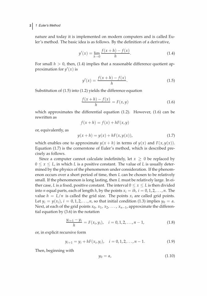
nature and today it is implemented on modern computers and is called Eu-ler’s method. The basic idea is as follows. By the definition of a derivative,

y′(x) = limh→0

f (x + h) − f (x)h

. (1.4)

For small h > 0, then, (1.4) implies that a reasonable difference quotient ap-proximation for y′(x) is

y′(x) =f (x + h) − f (x)

h. (1.5)

Substitution of (1.5) into (1.2) yields the difference equation

f (x + h) − f (x)h

= F(x, y) (1.6)

which approximates the differential equation (1.2). However, (1.6) can berewritten as

f (x + h) = f (x) + hF(x, y)

or, equivalently, asy(x + h) = y(x) + hF(x, y(x)), (1.7)

which enables one to approximate y(x + h) in terms of y(x) and F(x, y(x)).Equation (1.7) is the cornerstone of Euler’s method, which is described pre-cisely as follows.

Since a computer cannot calculate indefinitely, let x ≥ 0 be replaced by0 ≤ x ≤ L, in which L is a positive constant. The value of L is usually deter-mined by the physics of the phenomenon under consideration. If the phenom-enon occurs over a short period of time, then L can be chosen to be relativelysmall. If the phenomenon is long lasting, then L must be relatively large. In ei-ther case, L is a fixed, positive constant. The interval 0 ≤ x ≤ L is then dividedinto n equal parts, each of length h, by the points xi = ih, i = 0, 1, 2, . . . , n. Thevalue h = L/n is called the grid size. The points xi are called grid points.Let yi = y(xi), i = 0, 1, 2, . . . , n, so that initial condition (1.3) implies y0 = α.Next, at each of the grid points x0, x1, x2, . . . , xn−1, approximate the differen-tial equation by (3.6) in the notation

yi+1 − yi

h= F(xi, yi), i = 0, 1, 2, . . . , n − 1, (1.8)

or, in explicit recursive form

yi+1 = yi + hF(xi, yi), i = 0, 1, 2, . . . , n − 1. (1.9)

Then, beginning withy0 = α, (1.10)

1.2 Euler’s Method 3

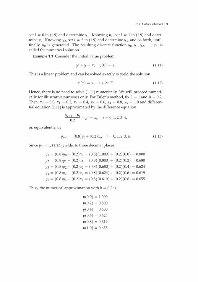
set i = 0 in (1.9) and determine y1. Knowing y1, set i = 1 in (1.9) and deter-mine y2. Knowing y2, set i = 2 in (1.9) and determine y3, and so forth, until,finally, yn is generated. The resulting discrete function y0, y1, y2, . . . , yn iscalled the numerical solution.

Example 1.1 Consider the initial value problem

y′ + y = x, y(0) = 1. (1.11)

This is a linear problem and can be solved exactly to yield the solution

Y(x) = x − 1 + 2e−x. (1.12)

Hence, there is no need to solve (1.11) numerically. We will proceed numeri-cally for illustrative purposes only. For Euler’s method, fix L = 1 and h = 0.2.Then, x0 = 0.0, x1 = 0.2, x2 = 0.4, x3 = 0.6, x4 = 0.8, x5 = 1.0 and differen-tial equation (1.11) is approximated by the difference equation

yi+1 − yi

0.2+ yi = xi, i = 0, 1, 2, 3, 4,

or, equivalently, by

yi+1 = (0.8)yi + (0.2)xi, i = 0, 1, 2, 3, 4. (1.13)

Since y0 = 1, (1.13) yields, to three decimal places

y1 = (0.8)y0 + (0.2)x0 = (0.8)(1.000)+ (0.2)(0.0) = 0.800

y2 = (0.8)y1 + (0.2)x1 = (0.8)(0.800)+ (0.2)(0.2) = 0.680

y3 = (0.8)y2 + (0.2)x2 = (0.8)(0.680)+ (0.2)(0.4) = 0.624

y4 = (0.8)y3 + (0.2)x3 = (0.8)(0.624)+ (0.2)(0.6) = 0.619

y5 = (0.8)y4 + (0.2)x4 = (0.8)(0.619)+ (0.2)(0.8) = 0.655.

Thus, the numerical approximation with h = 0.2 is

y(0.0) = 1.000

y(0.2) = 0.800

y(0.4) = 0.680

y(0.6) = 0.624

y(0.8) = 0.619

y(1.0) = 0.655.


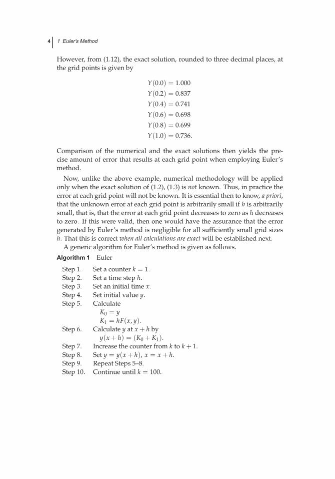
However, from (1.12), the exact solution, rounded to three decimal places, atthe grid points is given by

Y(0.0) = 1.000

Y(0.2) = 0.837

Y(0.4) = 0.741

Y(0.6) = 0.698

Y(0.8) = 0.699

Y(1.0) = 0.736.

Comparison of the numerical and the exact solutions then yields the pre-cise amount of error that results at each grid point when employing Euler’smethod.

Now, unlike the above example, numerical methodology will be appliedonly when the exact solution of (1.2), (1.3) is not known. Thus, in practice theerror at each grid point will not be known. It is essential then to know, a priori,that the unknown error at each grid point is arbitrarily small if h is arbitrarilysmall, that is, that the error at each grid point decreases to zero as h decreasesto zero. If this were valid, then one would have the assurance that the errorgenerated by Euler’s method is negligible for all sufficiently small grid sizesh. That this is correct when all calculations are exact will be established next.

A generic algorithm for Euler’s method is given as follows.

Algorithm 1 Euler

Step 1. Set a counter k = 1.Step 2. Set a time step h.Step 3. Set an initial time x.Step 4. Set initial value y.Step 5. Calculate

K0 = yK1 = hF(x, y).

Step 6. Calculate y at x + h byy(x + h) = (K0 + K1).

Step 7. Increase the counter from k to k + 1.Step 8. Set y = y(x + h), x = x + h.Step 9. Repeat Steps 5–8.Step 10. Continue until k = 100.

1.3 Convergence of Euler’s Method* 5

1.3Convergence of Euler’s Method*

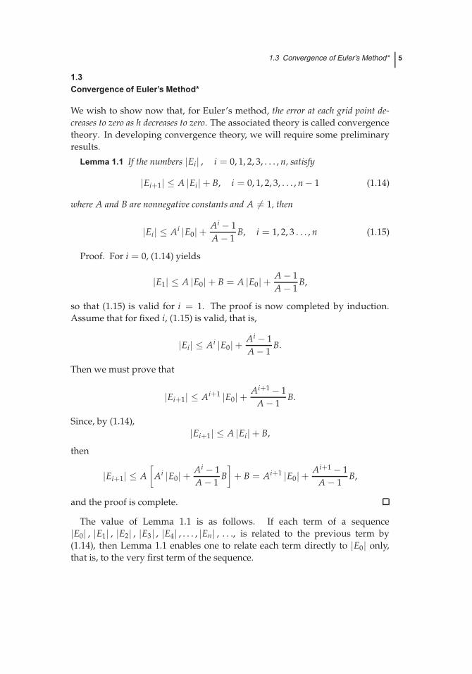
We wish to show now that, for Euler’s method, the error at each grid point de-creases to zero as h decreases to zero. The associated theory is called convergencetheory. In developing convergence theory, we will require some preliminaryresults.

Lemma 1.1 If the numbers |Ei| , i = 0, 1, 2, 3, . . . , n, satisfy

|Ei+1| ≤ A |Ei|+ B, i = 0, 1, 2, 3, . . . , n − 1 (1.14)

where A and B are nonnegative constants and A �= 1, then

|Ei| ≤ Ai |E0|+ Ai − 1A − 1

B, i = 1, 2, 3 . . . , n (1.15)

Proof. For i = 0, (1.14) yields

|E1| ≤ A |E0|+ B = A |E0|+ A − 1A − 1

B,

so that (1.15) is valid for i = 1. The proof is now completed by induction.Assume that for fixed i, (1.15) is valid, that is,

|Ei| ≤ Ai |E0|+ Ai − 1A − 1

B.

Then we must prove that

|Ei+1| ≤ Ai+1 |E0|+ Ai+1 − 1A − 1

B.

Since, by (1.14),|Ei+1| ≤ A |Ei|+ B,

then

|Ei+1| ≤ A[

Ai |E0| + Ai − 1A − 1

B]

+ B = Ai+1 |E0|+ Ai+1 − 1A − 1

B,

and the proof is complete.

The value of Lemma 1.1 is as follows. If each term of a sequence|E0| , |E1| , |E2| , |E3| , |E4| , . . . , |En| , . . ., is related to the previous term by(1.14), then Lemma 1.1 enables one to relate each term directly to |E0| only,that is, to the very first term of the sequence.


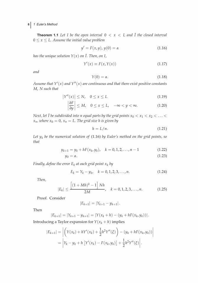
Theorem 1.1 Let I be the open interval 0 < x < L and I the closed interval0 ≤ x ≤ L. Assume the initial value problem

y′ = F(x, y), y(0) = α (1.16)

has the unique solution Y(x) on I. Then, on I,

Y′(x) ≡ F(x, Y(x)) (1.17)

andY(0) = α. (1.18)

Assume that Y′(x) and Y′′(x) are continuous and that there exist positive constantsM, N such that ∣∣Y′′(x)

∣∣ ≤ N, 0 ≤ x ≤ L (1.19)∣∣∣∣ ∂F∂y

∣∣∣∣ ≤ M, 0 ≤ x ≤ L, −∞ < y < ∞. (1.20)

Next, let I be subdivided into n equal parts by the grid points x0 < x1 < x2 < . . . <xn, where x0 = 0, xn = L. The grid size h is given by

h = L/n. (1.21)

Let yk be the numerical solution of (1.16) by Euler’s method on the grid points, sothat

yk+1 = yk + hF(xk, yk), k = 0, 1, 2, . . . , n − 1 (1.22)

y0 = α. (1.23)

Finally, define the error Ek at each grid point xk by

Ek = Yk − yk, k = 0, 1, 2, 3, . . . , n. (1.24)

Then,

|Ek| ≤[(1 + Mh)k − 1

]Nh

2M, k = 0, 1, 2, 3, . . . , n. (1.25)

Proof. Consider|Ek+1| = |Yk+1 − yk+1| .

Then|Ek+1| = |Yk+1 − yk+1| = |Y(xk + h) − (yk + hF(xk, yk))| .

Introducing a Taylor expansion for Y(xk + h) implies

|Ek+1| =∣∣∣∣(

Y(xk) + hY′(xk) +12

h2Y′′(ξ))− (yk + hF(xk, yk))

∣∣∣∣=

∣∣∣∣Yk − yk + h[Y′(xk) − F(xk, yk)

]+

12

h2Y′′(ξ)∣∣∣∣ .

1.3 Convergence of Euler’s Method* 7

From (1.17), then

|Ek+1| =∣∣∣∣Yk − yk + h [F(xk, Yk) − F(xk, yk)] +

12

h2Y′′(ξ)∣∣∣∣ ,

which, by the mean value theorem for a function of two variables, implies

|Ek+1| =∣∣∣∣Yk − yk + h

[(Yk − yk)

∂F∂y

(xk, η)]

+12

h2Y′′(ξ)∣∣∣∣

=∣∣∣∣(Yk − yk)

(1 + h

∂F∂y

)+

12

h2Y′′(ξ)∣∣∣∣ .

Hence, by the rules for absolute values,

|Ek+1| ≤ |Yk − yk|(

1 + h∣∣∣∣∂F

∂y

∣∣∣∣)

+12

h2 ∣∣Y′′(ξ)∣∣ ,

which, by (1.19), (1.20) yields

|Ek+1| ≤ |Yk − yk| (1 + Mh) +12

h2N.

Thus, since |Yk − yk|=|Ek|, one has

|Ek+1| ≤ |Ek| (1 + Mh) +12

h2N. (1.26)

Application of Lemma 1.1 to (1.26) with A = (1 + Mh), B = 12 h2N then im-

plies

|Ek| ≤ (1 + Mh)k |E0|+ (1 + Mh)k − 1(1 + Mh) − 1

(12

h2N)

. (1.27)

However, since Y(0) = y(0) = α, one has E0 = 0, so that (1.27) simplifies to

|Ek| ≤[(1 + Mh)k − 1

]Nh

2M, k = 0, 1, 2, 3, . . . , n, (1.28)

and the theorem is proved.

Theorem 1.2 Under the assumptions of Theorem 1.1, one has that at each gridpoint

limh→0

|Ek| = 0, k = 0, 1, 2, 3, . . . , n.

Proof. Since (1 + Mh) > 1, the largest value of (1 + Mh)k results whenk = n. Thus, from (1.28),

|Ek| ≤ [(1 + Mh)n − 1] Nh2M

, (1.29)


which, by (1.21), implies

|Ek| ≤[(1 + Mh)L/h − 1

]Nh

2M. (1.30)

By the laws of exponents, then,

|Ek| ≤

{[(1 + Mh)

1Mh

]ML − 1}

Nh

2M. (1.31)

Note now that if Mh = γ, then

limh→0

Mh = limγ→0

γ = 0.

Thus,

limh→0

[(1 + Mh)

1Mh

]ML= lim

γ→0

[(1 + γ)

1γ

]ML.

But, limγ→0

[(1 + γ)

1γ

]= e. Thus,

limh→0

{[(1 + Mh)

1Mh

]ML − 1}

Nh

2M= lim

h→0

{eML − 1

}Nh

2M= 0.

Thus, from (1.31), limh→0 |Ek| = 0 for all values of k, and the theorem isproved.

1.4Remarks

In practice, as will be shown soon, numerical methods which are more eco-nomical and more accurate than Euler’s method can be developed easily.However, convergence proofs for these methods are more complex than forEuler’s method.

Note that the essence of Theorem 1.2 is that if one wishes arbitrarily high ac-curacy, one need only choose h sufficiently small. Unfortunately, such remarksare purely qualitative. Indeed, if one has a prescribed accuracy, Theorems 1.1and 1.2 do not allow one to determine the precise h, a priori, since the constantN in (1.19) is rarely known exactly and the practical matter of roundoff errorin actual calculations has not been included in the theorems. The determina-tion of accuracy is often estimated in an a posteriori manner as follows. Onecalculates for both h and 1

2 h and takes those figures which are in agreementfor the two calculations. For example, if at a point x and for h = 0.1 one finds

1.5 Exercises 9

y = 0.876 532 while for h = 0.05 one finds at the same point that y = 0.876 513,then one assumes that the result y = 0.8765 is an accurate result.

As noted above, Theorems 1.1 and 1.2 do not consider roundoff error, whichis always present in computer calculations. At the present time there is nouniversally accepted method to analyze roundoff error after a large numberof time steps. The three main methods for analyzing roundoff accumulationare the analytical method (Henrici (1962), (1963)), the probabilistic method(Henrici (1962), (1963)) and the interval arithmetic method (Moore (1979)),each of which has both advantages and disadvantages.

1.5Exercises

1.1 With h = 0.1, find the numerical solution on 0 ≤ x ≤ 1 by Euler’s methodfor

y′ = y2 + 2x − x4, y(0) = 0.

and compare your results with the exact solution y = x2.


y′ = y3 − 8x3 + 2, y(0) = 0

and compare your results with the exact solution y = 2x.


y′ = xy2 − 2y, y(0) = 1.

Find the exact solution and compare the numerical results with it.


y′ = −2xy2, y(0) = 1,

and compare your results with the exact solution y = 11+x2 .


y′ = ey − ex2+ 2x, y(0) = 0,

and compare your results with the exact solution y = x2.


1.6 With h = 0.01, find the numerical solution on 0 ≤ x ≤ 10 by Euler’smethod for

y′ = y − 2 + x(1 + x)2 , y(0) = 1

and compare your results with the exact solution y = 11+x .

1.7 Estimate the value M in Theorem 1.1 for each of the following. If possible,also estimate the value of N.

(a) y′ = x + sin y, 0 < x < 1

(b) y′ = x2 cos y, 0 < x < 2

(c) y′ = x + y, 0 < x < 3.

Documents

Numerical Solution of Ordinary Differential Equations Greenspan Numerical Solution of Ordinary Differential Equations for Classical, Relativistic and Nano Systems WILEY-VCH Verlag