Embed Size (px)
Citation preview

Numerical Solutionof the Navier-Stokes Equations*
By Alexandre Joel Chorin
Abstract. A finite-difference method for solving the time-dependent Navier-
Stokes equations for an incompressible fluid is introduced. This method uses the
primitive variables, i.e. the velocities and the pressure, and is equally applicable to
problems in two and three space dimensions. Test problems are solved, and an ap-
plication to a three-dimensional convection problem is presented.
Introduction. The equations of motion of an incompressible fluid are
dtUi 4- UjdjUi = — — dip + vV2Ui + Ei} ( V2 = Yl d2 ) , djUj = 0 ,PO \ 3 '
where Ui are the velocity components, p is the pressure, p0 is the density, Ei are
the components of the external forces per unit mass, v is the coefficient of kinematic
viscosity, t is the time, and the indices i, j refer to the space coordinates Xi, x¡, i, j =
1, 2, 3. d, denotes differentiation with respect to Xi, and dt differentiation with
respect to the time t. The summation convention is used in writing the equations.
We write
, Uj , Xj , _ ( d \
Ui - u ' Xi " d ' p - \povur
e/ = ($)eí, f-(£),
where 77 is a reference velocity, and d a reference length. We then drop the primes.
The equations become
(1) dtu, 4- RujdjUi = —dip 4- V2u, + E, ,
(2) dfij = 0 ,
where R = Ud/v is the Reynolds number. It is our purpose to present a finite-
difference method for solving these equations in a bounded region 3), in either two-
or three-dimensional space. The distinguishing feature of this method lies in the
use of Eqs. (1) and (2), rather than higher-order derived equations. This makes it
possible to solve the equations and to satisfy the imposed boundary conditions
while achieving adequate computational efficiency, even in problems involving
three space variables and time. The author is not aware of any other method for
which such claims can be made.
Received February 5, 1968.
* The work presented in this report is supported by the AEC Computing and Applied Mathe-
matics Center, Courant Institute of Mathematical Sciences, New York University, under Con-
tract AT(30-1 )-1480 with the U. S. Atomic Energy Commission.
745
License or copyright restrictions may apply to redistribution; see http://www.ams.org/journal-terms-of-use

746 ALEXANDRE JOEL CHORIN
Principle of the Method. Equation (1) can be written in the form
(1)' dtUi + dip = <5nt ,
where CF.-w depends on u, and Ei but not on p; Eq. (2) can be differentiated to
yield
(2)' diidtUi) = 0.
The proposed method can be summarized as follows: the time t is discretized; at
every time step í¿ií is evaluated; it is then decomposed into the sum of a vector
with zero divergence and a vector with zero curl. The component with zero diver-
gence is dtUi, which can be used to obtain u,- at the next time level; the component
with zero curl is 3,-p. This decomposition exists and is uniquely determined when-
ever the initial value problem for the Navier-Stokes equations is well posed; it has
also been extensively used in existence and uniqueness proofs for the solution of
these equations (see e.g. [1]).
Let Ui, p denote not only the solution of (1) and (2) but also its discrete ap-
proximation, and let Du be a difference approximation to djU¡. It is assumed that
at time t = nAt a velocity field m," is given, satisfying Du" = 0. The task at hand
is to evaluate «<n+1 from Eq. (1), so that Dun+l — 0.
Let Tu i = buin+1 — Bu i approximate d¡w¿, where b is a constant and Bui a
suitable linear combination of Uin~>, j è 0. An auxiliary field w;aux is first evaluated
through
(3) &w¿aux — Buí = F{u
where F{u approximates íF.-w. w¿aux differs from utn+l because the pressure term
and Eq. (2) have not been taken into account. «,aux may be evaluated by an im-
plicit scheme, i.e. F At, may depend on u<n, w,aux and intermediate fields, say u*,
Ui**. bu?** — Bui now approximates í¿m to within an error which may depend
on Ai.Let Gip approximate dip. To obtain u¡n+l, p"+1 it is necessary to perform the
decomposition
Fíu = bus™ - But = Tut + Gipn+l, DQTu) = 0 .
It is, however, assumed that Dun~> = 0, j ^ 0. It is necessary therefore only
to perform the decomposition
(4) w¿aux = Uin+1 + b~lGipn+l,
where Duin+l = 0, and m,-"+1 satisfies the prescribed boundary conditions. Since
p" is usually available and is a good first guess for the values of pn+l, the decom-
position (4) is probably best done by iteration. For that purpose we introduce the
following iteration scheme :
(5a) u*+i.i*h - Miaux _ i)-'Gimp , m ^ 1 ,
(5b) p»+l,m+l _ pn+X,m _ \QUn+l,m+l ^ WI ä 1 ,
where X is a parameter, M,n+Im+1 and p"+1.™+1 are successive approximations to
Uin+l, pn+1, and Gimp is a function of pn+x-m+1 and p"+lm which converges to Gipn+l
as |pn+1.">+1 — p»+i.m| tends to zero. We set
License or copyright restrictions may apply to redistribution; see http://www.ams.org/journal-terms-of-use

NUMERICAL SOLUTION OF THE NAVIER-STOKES EQUATIONS 747
The iterations (5a) are to be performed in the interior of 2D, and the iterations
(5b) in 20 and on its boundary.
It is evident that (5a) tends to (4) if the iterations converge. We are using
dmp instead of dp in (5a) so as to be able to improve the rate of convergence of
the iterations. This will be discussed in detail in a later section. The form of Eq.
(5b) was suggested by experience with the artificial compressibility method [2]
where, for the purpose of finding steady solutions of Eqs. (1) and (2), p was re-
lated to Ui by the equation
dtp = constant • (âj-My) .
When for some I and a small predetermined constant e
„, n+X,l+X „n+l,î| ^max \p — p á £
we set
The iterations (5) ensure that Eq. (1), including the pressure term, is satisfied in-
side 3D, and Eq. (2) is satisfied in 3D and on its boundary.
The question of stability and convergence for methods of this type has not
been fully investigated. I conjecture that the over-all scheme which yields w,-n+1 in
terms of w," is stable if the scheme
Tu i = F ai
is stable. The numerical evidence lends support to this conjecture.
We shall now introduce specific schemes for evaluating tt¿aux and specific rep-
resentations for Du, dp, Gjmp. Many other schemes and representations can be
found. The ones we shall be using are efficient, but suitable mainly for problems
in which the boundary data are smooth and the domain 3D has a relatively simple
shape.
Evaluation of waux. We shall first present schemes for evaluating waux, defined
by (3).Equation (3) represents one step in time for the solution of the Burgers equation
dtUi = 3,-u ,
which can be approximated in numerous ways. We have looked for schemes which
are convenient to use, implicit, and accurate to 0(A7) + 0(Aa;2), where Ax is one
of the space increments Ax¿, i = 1, 2, 3. Implicit schemes were sought because
explicit ones typically require, in three space dimensions, that
At < iAx2
which is an unduly restrictive condition. On the other hand, implicit schemes of
accuracy higher than 0(Ai) would require the solution of nonlinear equations at
every step, and make it necessary to evaluate w,aux and ui"+1 simultaneously
License or copyright restrictions may apply to redistribution; see http://www.ams.org/journal-terms-of-use

748 ALEXANDRE JOEL CHORIN
rather than in succession. Since we assume throughout that Ai = 0(Aa;2), the gain
in accuracy would not justify the effort.
Two schemes have been retained after some experimentation. For both of them
Tu i = iuin+l - Uin)/At, Qj-1 = At, Buí = «¿"/Ai) .
They are both variants of the alternating direction implicit method.
(A) In two-dimensional problems we use a Peaceman-Rachford scheme, as
proposed by Wilkes in [3] in a different context. This takes the form
UHq,t) — Ui(q.r) — K . Wl(g,r)(M»(3+i,r) — Ui(q-X.r))
— ¿I ^ U2(1,r){Ui(q,r+X) — Ui{q,r-X))
(6a) +-~2 iu%+i,r) + M*(3-i,r) - 2u%,r))2Aii
+ T 2 iUi(,q,r+X) + Wi(,,r_l) — 2-U¿(3lI.))2Aa;2
aux _ * r> * / * * \Ui(z,r) — U¿(5,r) — 4Ar Ml^'r>^MiÍ9+1'rt ~~ Ui(q-l,r))
Ä^-t $ / aux aux \AAX M2(«'r'l-M''(«'r+1> — M«ï.r-1);
(6b) + T" h iu*(q+1,r) + M*(g-l,r) — M*(,,r))2Aa;i
+ &t / aux . aux r, aux \2 \M»"(í.r+l) I UHq,r-X) ~ ¿Unq,r))
2A^2
+ -£;,
where w¿* are auxiüary fields, and w,-(4,r) = UiiqAxx, rAx2). As usual, the one-
dimensional systems of algebraic equations can be solved by Gaussian elimination.
(B) In two-dimensional and three-dimensional problems we use a variant of
the alternating direction method analyzed by Samarskii in [4]. This takes the form
1t>i(qlT,s) — ^¿(q.r.s) O A'v ^1(3» r,s) V^'tif+l»»",«) ^i'(g— l,r,a))
~T" 2 V^íííf+l.r.s) ~T ^i(q-~l,r,s) ^Hq,r,8)) j
Mi(t,r,i) = tt¡to,r,j) — Ä ^T~T W2(«,r,«)lW,'(g,r+l,s) M ¿(3,r_l, s) J
_1_ * (■,,** J_ 1,** 9,/** "\"T 2 V.«*»(8,r+l,s) "T »¿(?,r-l,s) — ¿i*i(«,r,s);
Ax2
License or copyright restrictions may apply to redistribution; see http://www.ams.org/journal-terms-of-use
NUMERICAL SOLUTION OP THE NAVIER-SROKES EQUATIONS 749
aux _ jjcjs p &t £.£ . aux aux \
Mi(3,r,s) — Ui(gtT,s) Ä„, ít3(í,r,«) \MHq,T.t+l) Mj(5l,-,g_l)^
+ ^t / aux t aux q aux \2 lMí(9,r,s+l) "t" »¿(s,r,s-l) ¿W¿(9,,.,„))
Ax3
+ AtEi(q¡r¡a) ,
Ui(q,r,s) = Mi(gAxi, rAx2, sAz3),
Ei(Q,r,S) = EiiqAxx, rAx2, sAx3).
Ui*, U** are auxiliary fields. These equations can be written in the symbolic form
(7 - AiQiK*
(7) (7 - AÍQ,)«***(7 - AiQ3)Wiaux
where 7 is the identity operator, and Q¡ involves differentiations with respect to
the variable xi only.
It can be verified that when R = 0 scheme (6) is accurate to 0(Ai2) 4- 0(Ax2).
When Ä ^ 0 however, they are both accurate to the same order. Scheme (7) is
stable in three-dimensional problems; the author does not know of a simple ex-
tension of scheme (6) to the three-dimensional case. Scheme (7) has two useful
properties: It requires fewer arithmetic operations per time step than scheme (6),
and because of the simple structure of the right-hand sides, the intermediate fields
Ui*, ui** do not have to be stored separately.
If either scheme is to be used in a problem in which the velocities m¿"+1 are
prescribed at the boundary, values of u*, w¿**, w,aux at the boundary have to be
provided in advance so that the several implicit operators can be inverted. Con-
sider the case of the scheme (7). We have
Uin+1 = (7 + AtQx + AtQ2 4- AiQ3)u," 4- AtEi - AíG.-p» 4- 0(Aí2) ,
Ui* = (7 + AtQx)uin + 0(Ai2) ,
Ui** = (7 + AiQi + AtQ2)uin + 0(Ai2) ,
M.aux = (/+ AiQi 4- AíQ2 4- AtQ3)Uin + AtEt 4- 0(A<2) .
From these relations it can be deduced that if we set at the boundary
Ui* = Uin+X - AtQ2Uin+i - AtQsUin+1 - AtEi 4- AtGip ,
(8) ui** = Ui»+1 - AtQ3Uin+1 - AtEi + AtGip ,
ít¿aux = Uin+1 4- AtGip ,
the scheme will remain accurate to 0(A¿). Here Gi does not have to be identical
with d; all we need is
Gip" = dp" + O(Ai) .
The reason for introducing the new operator (?< is that at the boundary the normal
component of (?» has to be approximated by one-sided differences, while this is
not necessary in the interior of the domain 3D where Eq. (4) is assumed to hold.
More accurate expressions for the auxiliary fields at the boundaries can be
= uf,
= Ui* ,
= Ui** 4- AtEi,
License or copyright restrictions may apply to redistribution; see http://www.ams.org/journal-terms-of-use

750 ALEXANDRE JOEL CHORIN
used, provided one is willing to invest the additional programming effort required
to implement them on the computer. Appropriate expressions for u*, u?ux at the
boundary can be derived for use with the scheme (6).
It should be noted that for problems in which the viscosity is negligible, it is
possible to devise explicit schemes accurate to 0(A¿2) 4- 0(A.r2) and stable when
At = OiAx). Such schemes will be discussed elsewhere.
The Dufort-Frankel Scheme and Successive Point Over-Relaxation. In order
to explain our construction of D, G,m and our choice of X for use in (5a) and (5b),
we need a few facts concerning the Dufort-Frankel scheme for the heat equation
and its relation to the relaxation method for solving the Laplace equation.
Consider the equation
(9) -V2w = /, (V2 = dx2 + dx2)
in some nice domain 3D, say a rectangle, u is assumed known on the boundary of
3D. We approximate this equation by
(10) -Lu=f,where L is the usual five-point approximation to the Laplacian, and u and / are
now m-component vectors, m is the number of internal nodes of the resulting dif-
ference scheme. For the sake of simplicity we assume that the mesh spacings in the
Xx and x2 directions are equal, Axx = Ax2 — Ax; this implies no essential restric-
tion. The operator—L is represented by an m X m matrix A.
We write
A = A' - E - E'
where E, E' are respectively strictly upper and lower triangular matrices, and Ah
is diagonal. The convergent relaxation iteration scheme for solving (10) is defined
by
(11) (A' - co7>"+' = !(1 - u)A' + wE'}u» 4- uf
(see e.g. Varga [5]). co is the relaxation factor, 0 < w < 2, and the u" arc the suc^
cessive iterates. The evaluation of the optimal relaxation factor a!opt depends on
the fact that A satisfies "Young's condition (A)," i.e. that there exists a permuta-
tion matrix P such that
(12) P-lAP = A - A ,
where A is diagonal, and A has the normal form
(° °)\G' 0/
the zero submatrices being square. Under this condition, coopt can be readily de-
termined.
The matrix A depends on the order in which the components of w"+1 are com-
puted from un. Changing that order is equivalent to transforming A into I'~lAP,
where P is a permutation matrix.
We now consider the solution of (14) to be the asymptotic steady solution of
License or copyright restrictions may apply to redistribution; see http://www.ams.org/journal-terms-of-use

NUMERICAL SOLUTION OF THE NAVIER-STOKES EQUATIONS 751
(13) dTU=V2U+f
and approximate the latter equation by the Dufort-Frankel scheme
n+l n—X ¿il^T , n , n . n . n 0 «+1 on_1\ i o a tUq,r — Uq.r = -2 (."s+l.r + M«-l,r + W,i>r+i -f- M,,r_l — ¿Uq¡r — Zq,r ) + ¿At} ,
Ax
uq,T = u{qAxx, rAx2, nAr)
which approximates (13) when Ai = o(Ax). Grouping terms, we obtain
(14) Ar= 2- (Mg+l.r + Ma-I.r + Uq.r+l + Uq.r-x) + 2At/ .
Ax
Since m",, does not appear in (14), the calculation separates into two inde-
pendent calculations on intertwined meshes, one of which can be omitted. When
this is done, we can write
7Jn+1 = ( 2n+i ) (7J"+1 has m components) .
If we then write
(15) • r--§^/^1 4- 4Ar/ Ax
we see that the iteration (14) reduces to an iteration of the form (11) where the
new components of Un+l are calculated in an order such that A has the normal
form (12). The Dufort-Frankel scheme appears therefore to be a particular order-
ing of the over-relaxation method whose existence is equivalent to Young's con-
dition (A).
The best value of Ar, Aropt, can be determined from coopt and relation (15).
We find that Aropt = O(Ax), therefore for At = Aropt the Dufort-Frankel scheme
approximates, not Eq. (13), but rather the equation
dTu = V2u - 2 \~) d2u + f.
This is the equation which Garabedian in [6] used to estimate coopt. It can be used
here to estimate ATopt- These remarks obviously generalize to problems where
Azi 9e Ax2 or where there are more than two space variables.
The following remark will be of use: We could have approximated Eq. (13)
by the usual explicit formula
(16) uYr — Uq,r = -; (W«+I,r 4- K-l.r + K.r+X + w",r-l — 4:Uq,r) + Ar/Ax
and used this formula as an iteration procedure for solving (10). The resulting
iteration converges only when At/ Ax2 < 1/4, and the convergence is very slow.
The rapidly converging iteration procedure (14) can be obtained from (16) by
splitting the term w",r on the right-hand side into hiuYr + U"Y^-
License or copyright restrictions may apply to redistribution; see http://www.ams.org/journal-terms-of-use

752 ALEXANDRE JOEL CHORIN
Representation of D, d and 67, and the Iteration Procedure for Determining
w"+1, p"+1. For the sake of clarity we shall assume in this section that the domain
3D is two-dimensional and rectangular, and that the velocities are prescribed at the
boundary. Extension of the procedure to three-dimensional problems is immedi-
ate, and extension to problems with other types of boundary conditions often pos-
sible. Stress-free boundaries and periodicity conditions in particular offer no dif-
ficulty. Domains of more complicated shape can be treated with the help of ap-
propriate interpolation procedures.
Our first task is to define D. Let (B denote the boundary of 3D and Q the set of
mesh nodes with a neighbor in (B. In 3D — (B we approximate the equation of con-
tinuity by centered differences, i.e. we set
(17) Du =1
iUl(q+l,r) — Ux(q-X.r)) + («2(8,r+1) — M2(a,r-1)) — 02Azi ^i«"1'" ~™-"» i 2Az2
At the points of (B we use second-order one-sided differences, so that Du is
accurate to 0(Az2) everywhere. Consider the boundary line x2 = 0, represented
by j = 1 (Fig. 1). We have on that line
(18)
- -T~ [«2(5,2) — «2(5,1) — Ï («2(8,3) — «2(5,1))]
1
(mi(«+i,i) — «ks-i.d) — 0
Ax2
+2Azi
with similar expressions at the other boundaries. Equation (17) states that the
total flow of fluid into a rectangle of sides 2Axi, 2Az2 is zero. Equation (18) does
not have this elementary interpretation.
Figure 1. Mesh Near a Boundary.
We now define G ip at every point of 3D — (B by
GxV = 2^¡T (Pq+l.r - Pl-l.r) ,
G2p = 1^7 iVq,r+X - Pq.r-x) ,
Vq.r = piqAxx,rAx2) ,
i.e. dip is approximated by centered differences. It should be emphasized that
these forms of dp and Du are not the only possible ones.
License or copyright restrictions may apply to redistribution; see http://www.ams.org/journal-terms-of-use

NUMERICAL SOLUTION OF THE NAVIER-STOKES EQUATIONS 753
It is our purpose now to perform the decomposition (4). «"+1 is given on the
boundary (B, «¿aux is given in 3D — (B (the values of «¿aux on 03, used in (6) or (7),
are of no further use). pn+1 is to be found in 3D (including the boundary) and un+1
in 3D — 63, so that in 3D — 03
«¿aux = Uin+i 4- Atdp
and in 3D (including the boundary)
Dun+1 = 0 .
This is to be done using the iterations (5), where the form of dmp has not yet been
specified.
At a point (g, r) in 3D — 03 — C, i.e. far from the boundary, one can substitute
Eq. (5a) into Eq. (5b), and obtain
(19) pn+l,m+l _ pn+l.m = -\£)uau* _|_ M\DGmp .
This is an iterative procedure for solving the equation
(20) Lp = j^Ean \
where Lp = DGp approximates the Laplacian of p. With our choice of D and d,
Lp is a five-point formula using a stencil whose nodes are separated by 2 Axx, 2 Ax2.
Equation (20) is of course a finite-difference analogue of the equation
(21) V2p = didjUiUj 4- djEj,
which can be obtained from Eq. (1) by taking its divergence. At points of 03 or e
if it is not possible to substitute (5a) into (5b) because at the boundary «¿n+1 is
prescribed, w"+1"I+1 = wn+1 for all m, (5a) does not hold and therefore (19) is not
true. Near the boundary the iterations (5) provide boundary data for (20) and
ensure that the constraint of incompressibility is satisfied. We proceed as follows :
dmp and X are chosen so that (19) is a rapidly converging iteration for solving
(20); Gimp at the boundary are then chosen so that the iterations (5) converge
everywhere.
Let iq, r) again be a node in 3D — 03 — C. utn+l-m and pn+l'm are assumed
known. We shall evaluate simultaneously pY1,m+i and the velocity components
involved in the equation 7>u"+1 = 0 at iq, r), i.e. «h¿T,o, Ktl'ZtV) (FiS- 2)-These velocity components depend on the value of p at (q, r) and on the values
of p at other points. Following the spirit of the remark at the end of the last sec-
tion, the value of p at iq, r) is taken to be
UpZUm+1 + pZUm)
while at other points we use p"+Im.
This leads to the following formulae
(22a) pZUm+1 = pZUm - X7>w"+1'm+1
(7) given by (17))
/nrvu\ n+l,m+l aux ^t , nA~l,m \ / n-f-l.m-f-1 i n+l,m\\(22b) «1(8+1.r) = «1(8+1,r) - 2^T iPq+l.r - \iPq.r 4" Pq.r )) ,
License or copyright restrictions may apply to redistribution; see http://www.ams.org/journal-terms-of-use

754 ALEXANDRE JOEL CHORIN
(22c)
(22d)
(22e)
7i+l,m+] _ aux«1(9-1, r) — «1(8-1, r)
n+1,771+1
«2(5,7-+!)
aux«2(5,r+1) —
7i+l,77i+l aux«2(8, r-1) — «2(8, r-
At
2A.)j]
A¿
2Ax2
At
2Ax2
(iGC1'"*1+ „n-r-l,»n\ n+l,m\
Pq.r ) - Pq-i.r) ,
/ n+l,m i/ n+l,m+l , n+l,jn\\iPq.r+2 - hiPq.r 4- pq,r )) ,
i\iptr'm+l + pZUm) n-\-l,m\Pq.r-Y .
These equations define Gimp. Clearly, dmp —> G,p.
Equations (22) can be solved for p'Y/'m+l, yielding
71+1,771+1
(23a)p4,V" = (1 + ax + a2) '[(1 — ai — a2)pn+1,m — \Duu*
+ / n+l,m i n+l,»i\ ■ / n+l,m . n+l,m\iai(P8+2,r 4- Pg_2,r) 4- a2(pg,r+l 4- Pg,r_2)J ,
where a, = XA¿/4Aa,\, i = 1, 2. This can be seen to be a Dufort-Frankel relaxa-
tion scheme for the solution of (20), as was to be expected. The At of the preced-
ing section is replaced here by \At/2. Corresponding to Aropt (or coopt) wTe find
Xopt- If p were known on 03 and C, convergence of the iterations (23a) would follow
from the discussion in the preceding section, and X = Xopt would lead to the highest
rate of convergence.
ui(q-i,r)
9U2(q,r+l)
Pq.r>-°uKq+i,r)
°U2(q,r-i)
Figure 2. Iteration Scheme
In 03 and C formulae (22) are modified by the use of the known values of «,™+1
at the boundary whenever necessary. This leads to the formulae, for iq, r) in e :
(23b)pn+X.m+X = {l + ai+ la2)-'[(l _ ai _ ia2)pYYm - XD«a
+ / n+l,m | n+l,m\ ■ n+l,mi<*l(P5+2.2 4" Pq-i.i) + a2pqA ] ,
and for iq, r) on 03 :
71+1,771+1 /-, | \— If/, \ 71+1,771 -. 7-, BÜX
(23c) V"-1 (! + ai) Kl - ai)P8.i - >^7>m
2a2(P8.3 - \iPq.i — Pq.1 ))J
etc. In (23b) Du is given by (17), and in (23c) by (18). w,aux at the boundary is
interpreted as Uin+1. Although no proof is offered, a heuristic argument and the
numerical evidence lead us to state that the whole iteration system—Eqs. (23a),
(23b), (23c)—converges for all X > 0 and converges fastest when X ~ Xopt. None
of the boundary instabilities which arise in two-dimensional vorticity-stream func-
tion calculation has been observed.
It can be seen that because our representation of Du = 0 expresses the balance
of mass in a rectangle of sides 2Ax,, i = 1, 2, the pressure iterations split into
License or copyright restrictions may apply to redistribution; see http://www.ams.org/journal-terms-of-use

NUMERICAL SOLUTION OF THE NAVIER-STOKES EQUATIONS 755
two calculations on intertwined meshes, coupled at the boundary. The most effi-
cient orderings for performing the iterations are such that the resulting over-all
scheme is a Dufort-Frankel scheme for each one of the intertwined meshes. This
involves no particular difficulty; a possible ordering for a rectangular grid is shown
in Fig. 3. The iterations are to be performed until for some I
I 71+1, ¡+1 71+1, ¡I ^max \pYr + - pYr I Ú £
5.1-
for a predetermined e.
The new velocities W;n+I, i = 1, 2, are to be evaluated using (22b), (22c), (22d),
(22e). This has to be done only after the pn+l<m have converged. There is no need
to evaluate and store the intermediate fields «¿n+1'm+1. A saving in computing time
can be made by evaluating 7)«aux at the beginning of each iteration. We notice
two advantages of our iteration procedure: Dun+l can be made as small as one
wishes independently of the error in Dun; and when p"+li+1 and pn+1'1 differ by
less than e, Dun+1 = 0(f/X); it can be seen that Xopt = OiAxr1), hence Dun+1 =
0(£Ax). A gain in accuracy appears, which can be used to relax the convergence
criterion for the iterations. This gain in accuracy is due to the fact that the «¿"+1
are evaluated using an appropriate combination of pn+1-1 and p»+i.'+lt rather than
only the latest iterate p"+i,H-i<
F J D
I C K G A
The domain is swept in the order AB,CD,EF, GH,IJ,K
Figure 3. An Ordering for the Iteration Scheme
Solution of a Simple Test Problem. The proposed method was first applied to
a simple two-dimensional test problem, used as a test problem by Pearson in [7]
for a vorticity-stream function method. 3D is the square 0 í= x¿ ^ tt, i = 1, 2;
Ex — E2 = 0; the boundary data are
«i = —cos Xx sin x2e~~2', «2 = sin Xx cos x2e~2'.
The initial data are
License or copyright restrictions may apply to redistribution; see http://www.ams.org/journal-terms-of-use

756 ALEXANDRE JOEL CHORIN
ux = —cos xx sin x2, u2 = sin xx cos x2.
The exact solution of the problem is
«i = —cos xx sin x2e~2', u2 = sin xx cos x2e~2t,
p = —R Kcos 2xi 4- cos 2x2)e~u ,
where R is the Reynolds number. This solution has the property
dip = —RujdjUi ;
hence curl (w¿) satisfies a linear equation. Nevertheless, this problem is a fair test
of our method because 7)«aux ^ 0.
We first evaluate Xopt- For the equation
—Lu = f
in 3D, with a grid of mesh widths 2 Axx, 2 Ax2, and « known on the boundary, we
have
"opt-1 + (i-ay/2'
where a = |(cos 2Axi 4- cos 2Ax2) is the largest eigenvalue of the associated
Jacobi matrix (see [5]).
We put
q~ 2 \Axx2 Ax,2)'
Equation (15) can be written as
^1wopt — .
therefore
COopt ~ 14- 4g '
(X 2\l/2(1 - a )
and
iAt/Axx2 + Ai/Ace^) (1 - a2)1'2 '
We now assume Axx = A.r2 = Ax, obtaining
2Ax2«ont —
At sin (2Ax) '
In Tables I, II, and III we display results of some sample calculations, n is
the number of time steps; e(«¿), i = 1, 2, are the maxima over 3D of the differences
between the exact and the computed solutions w,-. It is not clear how the error in
the pressure is to be represented; pn is defined at a time intermediate between
(n — l)At and nAt; it is proportional to R in our nondimensionalization. There
License or copyright restrictions may apply to redistribution; see http://www.ams.org/journal-terms-of-use
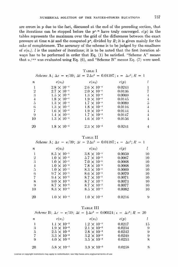
NUMERICAL SOLUTION OF THE NAVIER-STOKES EQUATIONS 757
are errors in p due to the fact, discussed at the end of the preceding section, that
the iterations can be stopped before the pn-m have truly converged. e(p) in the
tables represents the maximum over the grid of the differences between the exact
pressure at time nAt and the computed pn, divided by R; it is given mainly for the
sake of completeness. The accuracy of the scheme is to be judged by the smallness
of e{ui). I is the number of iterations; it is to be noted that the first iteration al-
ways has to be performed in order that Eq. (1) be satisfied. "Scheme A" means
that Miaux was evaluated using Eq. (6), and "Scheme B" means Eq. (7) were used.
Table I
Scheme A; Ax = tt/39; Ai = 2 Ax2 = 0.01397; e = Ax2; It = 1
n e(«i) e(w2) e(p) I
1 2.8 X 10⁻⁴ 2.6 X 10"4 0.0243 12 2.7 X 10⁻⁴ 2.0 X 10⁻⁴ 0.0136 73 1.5 X lO"4 1.3 X 10⁻⁴ 0.0069 44 1.8 X 10⁻⁴ 1.9 X lO"4 0.0145 45 1.3 X 10"4 1.7 X 10-' 0.0089 56 1.3 X 10⁻⁴ 1.8 X lO4 0.0116 47 1.6 X 10⁻⁴ 1.9 X 10⁻⁴ 0.0144 49 1.4 X 10⁻⁴ 1.7 X 10-" 0.0147 4
10 1.3 X 10"4 1.6 X 10 l 0.0156 4
20 1.8 X lO"4 2.3 X 10"4 0.0241 4
Table II
Scheme A; Ax = tt/39; Ai = 2A.r.2 = 0.01397; e = Ax3; R = 1
n eiux) e(«2) e(p) I
1 8.5 X 10⁻⁵ 3.8 X 10~5 0.0059 102 1.0 X 10"4 5.7 X 10⁻⁵ 0.0067 103 1.0 X 10⁻⁴ 7.0 X 10⁻⁶ 0.0068 104 1.0 X 10⁻⁴ 7.8 X 10⁻⁵ 0.0068 105 1.0 X 10⁻⁴ 8.3 X 10"5 0.0069 106 9.7 X 10⁻⁵ 8.6 X 10~5 0.0070 107 9.4 X lO"5 8.7 X 10"5 0.0071 108 9.0 X 10⁻⁵ 8.7 X 10⁻⁵ 0.0073 109 8.7 X 10"5 8.7 X lO"6 0.0077 10
10 8.3 X 10⁻⁵ 8.5 X 10"5 0.0082 10
20 1.0 X10⁻⁴ 1.0 X 10"4 0.0216 9
Table III
Scheme B; Ax = tt/39; At = ¿A.r2 = 0.00324; e = A.u2; R = 20
n e(«i) e(w2) e(p) I
1 1.1 X 10"3 1.2 X lO-3 0.0217 153 1.9 X 10"3 2.1 X 10"3 0.0234 95 2.5 X lO"3 2.8 X 10"3 0.0242 97 3.3 X lO"3 3.2 X 10"3 0.0249 99 4.0 X 10⁻³ 3.5 X lO"3 0.0253 8
20 5.8 X 10"3 3.9 X 10~3 0.0258 8
License or copyright restrictions may apply to redistribution; see http://www.ams.org/journal-terms-of-use

758 ALEXANDRE JOEL CHORIN
Tables I and II describe computations which differ only in the value of e.
They show that £ = Ax2 is an adequate convergence criterion. Table III indicates
that fair results can be obtained even when RAt is fairly large; when R = 20,
Ax = 7r/39, Ai = 2 A.r2, we have
£~ 1.5 Aar1.
The errors are of the order of 1 %. Additional computational results were presented
in [8].
Application to Thermal Convection. Suppose a plane layer of fluid, in the field
of gravity, of thickness d and infinite lateral extent, is heated from below. The
lower boundary x3 = 0 is maintained at a temperature T0, the upper boundary
Xi = d at a temperature Tx < T0. The warmer fluid at the bottom expands and
tends to move upward ; this motion is inhibited by the viscous stresses.
In the Boussinesq approximation (see e.g. [9]) the equations describing the
possible motions are
dtUi 4- UjdjUi = — —dip 4- eVV¿ - çy(l - (7 — 7'0))<5,-,Po
âtT 4- UjdjT = kV2T , d,Uj = 0 ,
where T is the temperature, k the coefficient of thermal conductivity, a the co-
efficient of thermal expansion, and 5, the components of the unit vector pointing
upwards.
We write
ut \v^> *■ To_ Ti , «
n> LÍ ±\n . (Tx - Tp)dgxi* ~ d ' P - p, \'y J P +
_C32
V
and drop the primes. The equations now are
R*dtUi 4- UjdjUi = —dip 4- VV¿ 4- — (7 — 1)5, ,
a
d,T-\-UjdjT = — Y2T , djUi = 0,
where R* = agd3irT0 — Tx)kv is the Rayleigh number, and <r = v/k the Prandtl
number. The rigid boundaries are now situated at x3 — 0 and xz = 1, where it is
assumed that w¿ = 0, i = 1, 2, 3.
It is known that for R* < R*, the state of rest is stable and no steady con-
vection can arise, where R* = 1707.762.
When R* = R*, steady infinitesimal convection can first appear, and the field
quantities are given by
us = CWixs)<t>,
CUi = -2 id3Wix3))di<t>, i = 1,2 ,
a
T = CTix3)<p
License or copyright restrictions may apply to redistribution; see http://www.ams.org/journal-terms-of-use

NUMERICAL SOLUTION OF THE NAVIER-STOKES EQUATIONS 759
where <p = <f>ixx, x2) determines the horizontal planform of the motion and satisfies
Oi2 + dt* 4- a2)tf» = 0 ,
Wix3), Tix3) are fully determined functions of x3, a = 3.117, and C is a small but
undetermined amplitude.
In two-dimensional motion ux = 0 and the motion does not depend on xx. We
then have
<p = cos ax2.
The motion is periodic in x2 with period 2-ir/a.
The Nusselt number Nu is defined as the ratio of the total heat transfer to the
heat transfer which would have occurred if no convection were present. For R*
^ R*, Nu = 1. In our dimensionless variables
A« = #- / * " (u3T - d3T)dx2.¿IT J 0
A similar expression holds in the three-dimensional case. When the convection is
steady A« does not depend on x3.
When R* > R* steady cellular convection sets in. It is of interest to determine
its magnitude and its spatial configuration. The problem of its magnitude, and in
particular the dependence of A« on R* and a, when the motion is steady, has been
studied by the author in previous work [2], [10]. As to the shape of the convection
cells, it is known that flows may exist in which the cells, when viewed from above,
look like hexagons, or like rectangles with various ratios of length to width, or like
rolls, i.e. two-dimensional convection cells (see [11]). However, only cellular struc-
tures which are stable with respect to small perturbations can persist in nature or
be exhibited by our method. It has been shown, numerically by the author [10],
experimentally by Koschmieder [12] and Rossby [13], theoretically, in the case of
infinite o- and small perturbations, by Busse [14], that for R*/Rc* < 10 the pre-
ferred cellular mode is a roll. Busse showed that the rolls are stable for wave num-
bers in a certain range. We shall now demonstrate numerically the impermanence
of hexagonal convection and the emergence of a roll.
Consider the case R*/R* = 2, o- = 1. We assume the motion to be periodic
in the xx and x% directions, with periods respectively 4tt/cz V 3 and 4tt/« (the first
period is apparently in the range of stable periods for rolls as predicted by Busse).
These are the periods of the hexagonal cells which could arise when R* = R*.
The state of rest is perturbed by adding to the temperature in the plane x3 = Aj3
a multiple of the function <f>ixx, x2) which corresponds to a hexagonal cell, and
adding a small constant to the temperature on the line xx — (3/4)(4x/a V3),
x2 = (3/4)(4,r/a). We then follow the evolution of the convection in time, using a
net of 24 X 24 X 25, i.e.
Axi = (4Tr/a V 3)/24 , A.r2 = (4Tr/a)/24 , Ax3 = 1/24 .
We choose e = Ax22, Ai = 3Ax32. The convection pattern is visualized as fol-
lows: the velocities in the plane x3 — 17A^3 are examined. If «3(8,r,is) > 0 an * is
printed, if u3iq,,,xs) ^ 0, a 0 is printed.
License or copyright restrictions may apply to redistribution; see http://www.ams.org/journal-terms-of-use

ALEXANDRE JOEL CHORIN
Figure 4. Evi
****** *000000000000000 * ******* *00000000000000000*******0000000000000**********00000000000000*0*** * * *00000000000000000 * * *
0000000000000000000000000000000000000000000000000000000000000000000000000000000000*0*00000000000000000000000000000000000000000 * * * * *0*000000000000000000000000000000000000000000000000000000000000000000000000000000000000000000000000000000000000000000000000000000000000000000000000000* * *000000000000000000000 * * *000000000000000000000 * * *00000000000000000000000000000000000000000000000000000000000000000000000000000000000000000000000000000000000000000000000000000
4a. After 1 step (Nu = 1)
********* *00000000000000***********000000000000************000000000000*
********** *ooooooooo * * * *
* * *0000000 **************
************* *ooooooo * * ************ *000000000000***********0000000000000
0********* *000000000000000 ********0000000000000000000 * * *00000000000000000000000000000 ****** *oooo00000000000***********0000000000000************00000000000 **************0000000000 **************0000000000 **************00000000000 *************000000000000**********0000000000000000000000000000* * * * * *00000000000000000******** *00000000000000
4c. After 125 steps (Nu = 1.25)
of a Convection Cell
******** *0000000000000 * *
********* *ooooooooo ************** *ooooooo ************** *ooooooooo ************ *000000000000 ******* * *000000000000000000 * * *
000000000000000000000000000000000 ****** *0000000000000************00000000000***********000000000000**********00000000000000********0000000000000oooo * * * * *00000000000000000000000000000000000000000000000000000000000000000000000000000* * * * * * *0000000000000000*********000000000000000 *********oo0000000000000*********0000000000000000 ****** *ooo00000000000000000000000000000*00000000000000000000**** *00000000000000000******* *0000000000000000
4b. After 10 steps (Nu = 1)
********* *00000000000000***********000000000000*
*********** *nooooooooo * ************* *qoooooooo * ************** *oooooooo * ***************oooooooo* ************** *oooooooo * ************* *oooooooooo ** * ** * ******* *QQQQQf)00000
00**********0000000000000000********0000000000000000000 * * * * *00000000000000000000 ****** *00000000000000000**********00000000000000 ************ *ooo00000000 ************* *Q()00000000 ************** *q00000000 ************** *n00000000 ************** *n
000000000 ************* *q00000000000***********0000000000000000000000000000000000000000000000000000 * * * * *00000000000000000
4d. After 225 steps (Nu = 1.72)
License or copyright restrictions may apply to redistribution; see http://www.ams.org/journal-terms-of-use

NUMERICAL SOLUTION OF THE NAVIER-STOKES EQUATIONS 761
0000 ******* *00000000000000************ooooooooooo************* *oooooooooo************** *ooooooooo************** *ooooooooo************** *oooooooo00**************00000000oo************ *000000000000************0000000000000***********00000000000000**********00000000000000**********00000000000000***********0000000000000* * ********* *000000000000 ************ *00000000000 ************ *0000000000 ************** *ooooo00000 ************* *0000000000 ************* *ooooo000000************0000000000000**********0000000000000000 ***** *000000000000000000000000000000000000000000000000000000000
4e. After 325 steps (Nu = 1.76)
0000***********0000000000000***********0000000000000***********0000000000000************00000000000 ************ *00000000000 ************ *00000000000 ************ *00000000000 ************ *000000000000***********0000000000000***********0000000000ooo***********ooooooooo0ooo***********ooooooooo0000***********0000000000000********** *000000000000************000000000000 ************ *oooooooo000 ************ *00000000000 ************ *000000000000***********0000000000000***********00000000000oo***********ooooooooo0000***********00000000000000*********000000000000000 ******** *0000000000
4f. After 430 steps (Nu = 1.77)
The evolution of the convection is shown in Figs. 4a, 4b, 4c, 4d, 4e, and 4f.
The hexagonal pattern introduced into the cell is not preserved. The system evolves
through various stages, and finally settles as a roll with period 4x/a V 3. The value
of Nu evaluated at the lower boundary is printed at the bottom of each figure.
The steady state value for a roll is 1.76. The final configuration of the system is
independent of the initial perturbation. The calculation was not pursued until a
completely steady state had been achieved because that would have been ex-
cessively time consuming on the computer. It is known from previous work that
steady rolls can be achieved, and that the mesh used here provides an adequate
representation.
Conclusion and Applications. The Benard convection problem is not considered
to be an easy problem to solve numerically even in the two-dimensional case. The
fact that with our method reliable time-dependent results can be obtained even
in three space dimensions indicates that the Navier-Stokes equations do indeed
lend themselves to numerical solution. A number of applications to convection
problems, with or without rotation, can be contemplated; in particular, it appears
to be of interest to study systematically the stability of Benard convection cells
when o- ¿¿ t», and when the perturbations have a finite amplitude.
Other applications should include the study of the finite amplitude instability
of Poiseuille flow, the stability of Couette flow, and similar problems.
Acknowledgements. The author would like to thank Professors Peter D. Lax
and Herbert B. Keller for their interest and for helpful discussions and comments.
License or copyright restrictions may apply to redistribution; see http://www.ams.org/journal-terms-of-use

762 ALEXANDRE JOEL CHORIN
New York University
Courant Institute of Mathematical Sciences
New York, New York 10012
1. H. Fujita & T. Kato, "On the Navier-Stokes initial value problem. I," Arch. RationalMech. Anal, v. 16, 1964, pp. 269-315. MR 29 #3774.
2. A. J. Chorin, "A numerical method for solving incompressible viscous flow problems,"J. Computational Physics, v. 2, 1967, p. 12.
3. J. O. Wilkes, "The finite difference computation of natural convection in an enclosedcavity," Ph.D. Thesis, Univ. of Michigan, Ann Arbor, Mich., 1963.
4. A. A. Samarskii, "An efficient difference method for solving a multi-dimensional para-bolic equation in an arbitrary domain," Z. Vycisl. Mat. i Mat. Fiz., v. 2, 1962, pp. 787-811 =U.S.S.R. Comput. Math, and Math. Phys., v. 1963, 1964, no. 5, pp. 894-926. MR 32 #609.
5. R. Varga, Matrix Iterative Analysis, Prentice-Hall, Englewood Cliffs, N. J., 1962.6. P. R. Garabedian, "Estimation of the relaxation factor for small mesh size," Math.
Comp., v. 10, 1956, pp. 183-185. MR 19, 583.7. C. E. Pearson, "A computational method for time dependent two dimensional incom-
pressible viscous flow problems," Report No. SBRC-RR-64-17, Sperry Rand Research Center,Sudbury, Mass., 1964.
8. A. J. Chorin, "The numerical solution of the Navier-Stokes equations for incompressiblefluid," AEC Research and Development Report No. NYO-1480-82, New York Univ., Nov. 1967.
9. S. Chandrasekhar, Hydrodynamic and Hydromagnetic Stability, Internat. Series of Mono-graphs on Physics, Clarendon Press, Oxford, 1961. MR 23 #1270.
10. A. J. Chorin, "Numerical study of thermal convection in a fluid layer heated from below,"AEC Research and Development Report No. NYO-1480-61, New York Univ., Aug. 1966.
11. P. H. Rabinowitz, "Nonuniqueness of rectangular solutions of the Benard problem,"Arch. Rational Mech. Anal. (To appear.)
12. E. L. Koschmieder, "On convection on a uniformly heated plane," Beitr. Physik. Ahn.,v. 39, 1966, p. 1.
13. H. T. Rossby, "Experimental study of Benard convection with and without rotation,"Ph.D. Thesis, Massachusetts Institute of Technology, Cambridge, Mass., 1966.
14. F. Busse, "On the stability of two dimensional convection in a layer heated from below,"J. Math. Phys., v. 46, 1967, p. 140.
License or copyright restrictions may apply to redistribution; see http://www.ams.org/journal-terms-of-use