Embed Size (px)
Citation preview

Drag Minimization Based on the Navier-Stokes
Equations Using a Newton-Krylov Approach
Lana Osusky1, Howard Buckley 2, Thomas Reist 3, and David W. Zingg4
University of Toronto, Toronto, Ontario, M3H 5T6, Canada
A methodology is presented for performing numerical aerodynamic shape optimiza-
tion based on the three-dimensional Reynolds-averaged Navier-Stokes (RANS) equa-
tions. An initial multi-block structured mesh is first fit with B-spline volumes which
form the basis for a hybrid mesh movement scheme that is tightly integrated with the
geometry parameterization based on B-spline surfaces. The RANS equations and the
one-equation Spalart-Allmaras turbulence model are solved in a fully coupled manner
using an efficient parallel Newton-Krylov algorithm with approximate-Schur precondi-
tioning. Gradient evaluations are performed using the discrete-adjoint approach with
analytical differentiation of the discrete flow and mesh movement equations. The over-
all methodology remains robust even in the presence of large shape changes. Several
examples of lift-constrained drag minimization are provided, including a study of the
Common Research Model (CRM) wing geometry, a wing-body-tail geometry with a
prescribed spanwise load distribution, and a Blended-Wing-Body (BWB) configura-
tion. An example is provided that demonstrates that a wing optimized based on the
Euler equations exhibits substantially inferior performance when subsequently ana-
lyzed based on the RANS equations relative to a wing optimized based on the RANS
equations.
1 Member AIAA (currently Mechanical Engineer, GE Global Research)2 Research Associate, University of Toronto Institute for Aerospace Studies3 Ph.D. Candidate, University of Toronto Institute for Aerospace Studies4 Professor and Director, Tier 1 Canada Research Chair in Computational Fluid Dynamics and Environmentally
Friendly Aircraft Design, J. Armand Bombardier Foundation Chair in Aerospace Flight, AIAA Associate Fellow.
1

Nomenclature
A flow Jacobian matrix
b vector of control point coordinates (volume)
Bijk control point coordinates (local node)
c vector of constraints
CD coefficient of drag
CL coefficient of lift
CM coefficient of pitching moment
Cp coefficient of pressure
d distance to closest surface boundary
E Young’s modulus
E, F, G inviscid flux vectors
Ev, Fv, Gv viscous flux vectors
f force vector
g vector of computational mesh coordinates
J objective function
K stiffness matrix
L Lagrangian function
m number of mesh movement increments
m vector of metric terms
M Mach number
M mesh movement residual vector
Ni, Nj , Nk number of B-spline control points in each coordinate direction
N B-spline basis function
q vector of conservative flow variables (mesh volume)
Q vector of conservative flow variables (local node)
R flow residual vector
Re Reynolds number
T knot vector
v,X design variable vectors
λ(i) vector of mesh adjoint variables at increment i
ψ vector of flow adjoint variables
2

ν Poisson’s ratio
ν turbulence variable
ξ, η, ζ computational coordinate axes
I. Introduction
RISING fuel prices, along with stricter environmental regulations, have contributed to a push
within the airline industry for more efficient aircraft that will alleviate fuel costs and reduce green-
house gas emissions. The next generation of more fuel-efficient aircraft may be the result of in-
cremental improvements to the conventional tube-and-wing configuration [1, 2] or a novel design
not yet discovered. In either case, numerical analysis and optimization will be a powerful tool in
the design of new aircraft with a reduced environmental footprint. Numerical methods are already
being used in the design of the unconventional blended wing-body, double-bubble, and joined-wing
configurations [3–7].
The earliest examples of numerical aerodynamic shape optimization can be found in the work of
Hicks and Henne [8], who employed finite-difference gradient evaluations and inviscid flow analysis.
The use of finite-difference approximations to compute the gradient limited their optimizations to a
relatively low number of design variables. The size of the design problem was able to be increased
substantially with the advent of adjoint-based methods [9, 10], which make the cost of the gradient
evaluation virtually independent of the number of design variables. Since this pioneering work,
numerical aerodynamic optimization has become a growing area of research, encompassing a wide
variety of design problems with varying degrees of geometric variation relative to an initial geom-
etry. For example, in aerodynamic optimization typical of the detailed design phase, incremental
improvements are sought by implementing small-scale changes in the initial geometry. In high-
fidelity aerostructural and multidisciplinary optimization, for which an effective aerodynamic shape
optimization methodology is an essential component, a wing or aircraft will typically encounter
large changes in twist and planform. Finally, in exploratory optimization, the designer often has
no knowledge of the types of geometries the optimizer may produce; consequently, very large shape
changes can be encountered, and the optimization methodology must be capable of handling them.
The discrete-adjoint approach has been successfully used in a wide range of two-dimensional
3

aerodynamic shape optimization problems based on the Reynolds-averaged Navier-Stokes (RANS)
equations. Anderson and Bonhaus [11] applied the discrete-adjoint gradient evaluation approach
to airfoil section optimization problems on unstructured grids in fully turbulent flow; the one-
equation Spalart-Allmaras turbulence model was coupled with the Navier-Stokes equations and was
fully linearized. Nemec and Zingg [12, 13] developed an efficient gradient-based Newton-Krylov
scheme which has been applied to a wide range of two-dimensional turbulent aerodynamic shape
optimization problems [14]. Laminar-turbulent transition prediction was incorporated into this tool
by Driver and Zingg [15] and used to design a series of natural-laminar-flow airfoils.
Gradient-based three-dimensional turbulent aerodynamic shape optimization is also an active
and growing area of research. Hicken and Zingg [16] previously demonstrated the performance of
a gradient-based optimization tool based on the three-dimensional Euler equations but pointed out
the importance of considering viscous and turbulent effects in order to design under more realistic
flow conditions. Elliott made similar assertions in his thesis on optimization based on the two- and
three-dimensional Euler and laminar Navier-Stokes equations [17, 18]. Jameson et al. [19] used the
continuous adjoint approach in the development of SYN107 to optimize wings and wing-body config-
urations based on the compressible Navier-Stokes equations. Nielsen and Anderson [20] presented
examples of discrete-adjoint based optimization based on the three-dimensional RANS equations
and the Spalart-Allmaras turbulence model and showed the negative impact that certain simplifi-
cations of the linearization have on the gradient accuracy, including freezing the turbulence model.
Brezillon et al. [21] demonstrated improved performance of the DLR-F6 wing-body configuration
with an approach based on the unstructured parallel RANS solver, TAU, and discrete-adjoint gra-
dients; this work was extended to show how the optimization algorithm can be used to reduce the
area of flow recirculation at a wing-body junction and to optimize the slat and flap positions for a
three-dimensional high-lift configuration [22].
A good summary of the state of the art of RANS-based aerodynamic shape optimization is
provided by Epstein et al. [23], who applied three state-of-the-art optimization methodologies to
the same constrained design problem and demonstrated similar improvements in drag at the main
design point and good performance at off-design conditions. Note, however, that the shape changes
4

in the design problem used in their study are quite small, and no indication is given as to how
the methodologies would perform in an optimization with larger shape changes. Overall, RANS-
based aerodynamic shape optimization usually involves small changes typical of optimization in the
detailed design phase; RANS-based optimization involving large shape changes is still quite rare
and requires further research.
Aerostructural and multidisciplinary optimization have been in use for many years [24, 25];
however, the computational costs associated with RANS-based optimization make examples of high-
fidelity RANS-based aerostructural and multidisciplinary optimization quite rare. Jameson’s work
was extended to aero-structural wing planform optimizations [26]. Martins et al. [27] applied an
aerodynamics model based on the Euler equations and a finite-element structures model to the op-
timization of a natural-laminar-flow supersonic business jet. Kenway and Kennedy [28, 29] demon-
strated a parallelized high-fidelity multidisciplinary algorithm based on an Euler-based flow analysis
tool and a finite-element structures model to optimize the CRM aircraft configuration for minimum
fuel burn and, separately, minimized maximum take-off weight. Multi-point optimizations were also
presented. Recently, Barcelos et al. demonstrated the performance of an aerostructural optimiza-
tion methodology based on the RANS equations [30]. Ghazlane et al. [31] applied an aerostructural
adjoint method to aerodynamic, aeroelastic, and structural optimizations of the Airbus XRF1 wing-
body configuration at a single manoeuvre condition. A multidisciplinary methodology capable of
small- and large-scale shape changes based on high-fidelity analysis of aerodynamics, aeroelasticity,
structures, and acoustics is in development by Brezillon et al. [32] and has been demonstrated for
a regional jet configuration with rear fuselage-mounted engines.
This paper describes a methodology for performing aerodynamic shape optimization in tur-
bulent flow. By coupling an integrated geometry parameterization and mesh movement technique
with an efficient parallel Newton-Krylov-Schur method for solving the three-dimensional RANS
equations, this methodology is effective not only in optimizations typical of the detailed design
phase in which incremental improvements are sought, but also in cases with large shape changes.
The geometric flexibility and robustness that enables the optimizer to accommodate such a wide
range of shape changes will make this methodology a powerful tool as part of a future aerostructural
5
and multidisciplinary framework, as well as in exploratory optimization.
The paper is divided into the following sections. Section II outlines the integrated geometry
parameterization and mesh movement scheme, Section III describes the Newton-Krylov-Schur flow
solution algorithm, and Section IV provides details of the discrete-adjoint gradient evaluation. Re-
sults are presented in Section V for several optimization studies, including an optimization of the
Common Research Model wing geometry, an example in which large geometry changes are encoun-
tered, a wing-body-tail configuration where a prescribed spanwise loading constraint is imposed,
and a blended wing-body configuration. Conclusions are given in Section VI.
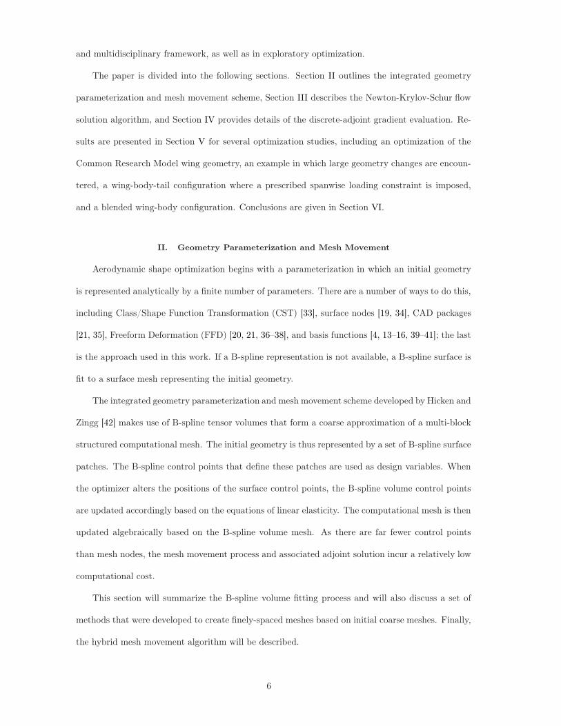
II. Geometry Parameterization and Mesh Movement
Aerodynamic shape optimization begins with a parameterization in which an initial geometry
is represented analytically by a finite number of parameters. There are a number of ways to do this,
including Class/Shape Function Transformation (CST) [33], surface nodes [19, 34], CAD packages
[21, 35], Freeform Deformation (FFD) [20, 21, 36–38], and basis functions [4, 13–16, 39–41]; the last
is the approach used in this work. If a B-spline representation is not available, a B-spline surface is
fit to a surface mesh representing the initial geometry.
The integrated geometry parameterization and mesh movement scheme developed by Hicken and
Zingg [42] makes use of B-spline tensor volumes that form a coarse approximation of a multi-block
structured computational mesh. The initial geometry is thus represented by a set of B-spline surface
patches. The B-spline control points that define these patches are used as design variables. When
the optimizer alters the positions of the surface control points, the B-spline volume control points
are updated accordingly based on the equations of linear elasticity. The computational mesh is then
updated algebraically based on the B-spline volume mesh. As there are far fewer control points
than mesh nodes, the mesh movement process and associated adjoint solution incur a relatively low
computational cost.
This section will summarize the B-spline volume fitting process and will also discuss a set of
methods that were developed to create finely-spaced meshes based on initial coarse meshes. Finally,
the hybrid mesh movement algorithm will be described.
6

A. Fitting Geometries and Multi-Block Meshes Using B-Spline Surfaces and Volumes
A B-spline tensor volume is defined by a set of control points, Bijk, and basis functions of order
p = 4, N , and can be expressed as
x(ξ) =
Ni∑
i=1
Nj∑
j=1
Nk∑
k=1
BijkNi (ξ)Nj (η)Nk (ζ) , (1)
where x (ξ) represents the set of Cartesian coordinates of the nodes of the mesh volume as a function
of the set of curvilinear coordinates ξ = (ξ, η, ζ) ∈ R3|ξ, η, ζ ∈ [0, 1]. The basis functions in the
ξ-direction, holding the η and ζ parameters constant, are expressed as
N(1)i (ξ; η, ζ) =
1 if Ti(η, ζ) ≤ ξ < Ti+1(η, ζ),
0 otherwise
(2)
N(p)i (ξ; η, ζ) =
(
ξ − Ti(η, ζ)
Ti+p−1(η, ζ)− Ti(η, ζ)
)
N(p−1)i (ξ; η, ζ)
+
(
Ti+p(η, ζ)− ξ
Ti+p(η, ζ)− Ti+1(η, ζ)
)
N(p−1)i+1 (ξ; η, ζ).
Similar expressions exist for the basis functions in the η- and ζ-directions, N(p)j (η; ζ, ξ) and
N(p)k (ζ; ξ, η), respectively. The parameter values (ξ, η, ζ) are determined using a chord length pa-
rameterization.
The spatially-varying knot values, Ti(η, ζ), in the interior of the B-spline volume are obtained
from
Ti(η, ζ) = [(1− η)(1 − ζ)]Ti,(0,0) + [η(1 − ζ)]Ti,(1,0) + [(1− η)ζ]Ti,(0,1) + [ηζ]Ti,(1,1), (3)
with similar expressions used for Ti(ζ, ξ) and Ti(ξ, η). The edge knot values, Ti,(0,0), Ti,(1,0), Ti,(0,1),
and Ti,(1,1) are constants and, since they are calculated based on the chord-length-based parameter
values, also possess a chord-length parameterization.
The initial locations of the B-spline control points are determined using a least-squares fitting
routine, which sequentially fits block edges, followed by surfaces and, finally, the internal volume
control points. The subset of B-spline control points associated with the aerodynamic surface are
7

typically used as design variables in an optimization.
B-spline curves obey a strong convex hull property which dictates that a point on a curve of
order p must be contained within the convex hull formed by p of its neighbouring control points.
Additionally, the movement of a particular control point will produce only localized changes in the
curve, which provides local shape control [43]. These properties result in a set of B-spline control
points that not only define the computational volume mesh, but also form an approximation of it.
This is an important principle that forms the basis for the mesh movement algorithm.
B. Mesh Refinement Techniques for Turbulent Flow Analysis and Optimization
A computational mesh used in a RANS-based analysis requires fine spacings, particularly in the
off-wall direction, in order to accurately capture turbulent flow features, such as the boundary layer.
In an Euler-based analysis, the computational mesh may have an off-wall spacing of approximately
10−3 reference units, whereas that of a mesh used in a RANS-based analysis is approximately 10−6
reference units. Some additional refinement (approximately one order of magnitude compared to
a coarser Euler mesh) is required in the tangential directions on the aerodynamic surfaces as well.
Problems arise when fitting the finer computational meshes due to the use of the spatially-varying
knot vectors based on the chord length-based parameter values, which cause the B-spline control
points to bunch together, and even cross over, in areas near the aerodynamic surface, where the
spacings are very fine or where there is a high amount of curvature, and produces a mesh of poor
quality. A balance must be struck between creating a well-spaced control-volume mesh and a fitted
computational mesh with a sufficient degree of refinement for modelling turbulent flow.
To this end, a dual-option refinement process has been developed that enables grid refinement
and redistribution by exploiting the parametric space associated with the B-spline volume. For
a given geometry, a computational mesh with coarser spacing is generated. At the beginning of
an optimization, each block of the computational mesh is fit with B-spline volumes using a least-
squares fitting routine, as previously discussed in Section II A. The coarser computational mesh
spacing eliminates bunching and cross-over in the resulting B-spline control-volume mesh. After the
B-spline control-volume mesh has been generated, the mesh can be refined using a node-insertion
8

method, which is referred to as grid refinement. The grid refinement option increases the number
of nodes in each coordinate direction by user-specified scaling factors. The entire set of parameter
values is re-evaluated using the chord-length based parameterization such that the existing nodes
are redistributed to account for the additional nodes.
The second option, which is referred to as grid redistribution, involves the targeted modification
of the spacing-control function parameters along specific grid edges. Starting with any fitted compu-
tational mesh (which may or may not have already made use of the grid refinement option), the edge
spacing parameters corresponding to specific blocks can be adjusted by a set of user-defined scaling
factors. This effectively creates spacing refinement by altering the distribution of the nodes along
an edge, rather than by inserting additional nodes. The parameter values ξ = (ξ, η, ζ) throughout
the remainder of the grid volume are re-evaluated based on the updated edge parameters so that
only the block edge spacing parameters need to be altered in order to achieve a distributed grid
spacing modification.
A third method, referred to as parameter extraction, has also been implemented. It makes
use of a finely-spaced turbulent computational mesh that is canonically equivalent to the coarser
mesh and already contains the desired mesh spacing. The grid is read in and the parameter values
extracted and applied to the coarser initial mesh; this serves as a variation on the grid redistribution
scheme. Instead of manually refining the edge parameter spacings, the nodes of the entire mesh are
effectively redistributed based on the turbulent mesh. The cases presented in this work make use
of both the grid redistribution method and the parameter extraction method; the method used in
each case presented in this work will be explicitly stated.
Since the refinement strategies presented here are all performed in parametric space after the
B-spline control-volume mesh has been calculated, any refinement that is performed on the coarse
mesh in order to obtain the desired grid spacings has no effect on the control mesh.
C. Hybrid Mesh Movement
A set of design variables will be updated at each iteration of the optimization. The design
variables are typically the coordinates of the surface B-spline control points, referred to as section
9

shape variables, as well as the angle of attack and planform variables, such as sweep. Planform
variables are formed by coupling the coordinates of the B-spline control points; for example, the
x-coordinates of the surface control points can be coupled to form a single sweep planform variable.
Any changes in the control-point coordinates due to the modification of planform variables are
independent of the section shape variable changes so that, even if the sections are fixed, the planform
variables can still change. Modifications to the surface geometry specified by the optimizer must
subsequently be propagated through the B-spline volumes. To achieve this, a method based on
the principles of linear elasticity was adapted from the work of Truong et al. [44] by Hicken and
Zingg [42]. This type of method is computationally expensive; however, the size of the control mesh
is typically two orders of magnitude smaller than the flow mesh and thus its movement requires
minimal computational time compared to the time required to perform a flow analysis.
The control volumes are modelled as homogeneous, isotropic linear elastic solids, The movement
of the control points is governed by
∂τij∂xj
+ fi = 0, (4)
where fi is a force vector. The stress tensor, τij , and the Cauchy strain tensor eij , are related by
the linear expression
τij =E
1 + ν
(
eij +νekkδij1− 2ν
)
(5)
eij =1
2
(
∂ui
∂xj
+∂uj
∂xi
)
(6)
where u represents displacement, E is the spatially-varying Young’s modulus, and ν = −0.2 is
Poisson’s ratio. This approach assumes that the displacements are small; however, to accommodate
larger shape changes, the mesh movement is performed in increments, improving the robustness of
the method. Five mesh movement increments of equal size are used (m = 5). The choice of five
increments is neither necessary nor sufficient to ensure that high quality meshes are obtained in
all cases. However, we have found this value to be a good balance between speed and robustness
10

for many optimization problems of interest. The spatially-varying Young’s modulus for a given
mesh element, ε, at mesh movement increment i is expressed as a function of cell volume and cell
orthogonality, or skewness:
E(i)ε =
Φ(i−1)ε
Φ(0)ε V
(i−1)ε
, i = 1, 2, . . . ,m, (7)
where Vε is the element volume and Φε is a cell orthogonality measure. The Young’s modulus is
based on the cells of the control mesh. In order for this approach to be effective, these must reflect
those of the flow mesh.
Equation (4) is discretized on the control mesh using a finite-element method with trilinear
elements. Incorporating the incremental mesh movement results in the linear system
M(i)(b(i−1),b(i)) = K(i)(b(i−1))[b(i) − b(i−1)]− f (i) = 0, i = 1, . . . ,m, (8)
where M(i) is the mesh movement residual at increment i, K(i) is the sparse, symmetric, positive-
definite stiffness matrix, b(i) is a block-column vector containing the control-point coordinates at
increment i, and f (i) is a force vector that is defined implicitly based on the movement of the
control points on the aerodynamic surfaces. A node associated with a deformed boundary has a
force contribution equal to the product of its element stiffness and its displacement. The remaining
entries in the force vector are zero. Note that the term Bijk in (1) represents a set of coordinates for a
single control point, a lower-case b term in (8) represents a block-column vector of the coordinates
for all control points within a B-spline volume, and bs represents a subset of b, containing the
surface control-point coordinates.
The linear system (8) is solved using the conjugate gradient method preconditioned with ILU(1)
[45]. The convergence criterion is a reduction in the L2 norm of the residual to a relative tolerance
of 10−12. The fine mesh is updated using an algebraic approach based on the B-spline volume
basis functions in (1). This integrated approach remains efficient even for large multi-block meshes,
requiring minimal CPU time for the mesh movement and mesh adjoint systems relative to the time
required to solve the flow and compute the gradient, while maintaining good mesh quality. The
11
mesh adjoint system will be discussed in more detail in Section IV.
III. Newton-Krylov-Schur Flow Solver
At its core, an optimization algorithm must have an efficient, accurate method of analyzing the
flow around an aerodynamic body. Given inaccurate data from the flow solver, the optimizer can
not produce a valid optimum for the specified flow conditions. Efficiency and robustness are key
attributes of the flow solver, since the flow analysis is carried out many times over the course of
an optimization, and the geometry can be expected to undergo large changes in many cases. The
Newton-Krylov-Schur method used to obtain the flow solutions for the high-fidelity aerodynamic
shape optimization algorithm will be summarized briefly in this section. The parallel implicit flow
solution algorithm was developed by Hicken and Zingg [46] for the solution of the three-dimensional
Euler equations and adapted by Osusky and Zingg [47] to solve the three-dimensional Reynolds-
Averaged Navier-Stokes equations.
The algorithm solves the three-dimensional Reynolds-averaged Navier-Stokes (RANS) equa-
tions, given in curvilinear coordinates by [48]
∂tQ+ ∂ξE+ ∂ηF+ ∂ζG =1
Re
(
∂ξEv + ∂ηFv + ∂ζGv
)
, (9)
where the inviscid fluxes are represented by E, F, and G, and the viscous fluxes by Ev, Fv, and Gv.
The vector Q represents the set of conservative flow variables. The Spalart-Allmaras turbulence
model adds an additional variable and partial differential equation; it is treated in a fully-coupled
manner.
The governing equations are discretized on multi-block structured grids using second-order-
accurate summation-by-parts (SBP) operators. Boundary conditions and inter-block coupling are
enforced weakly using simultaneous approximation terms (SATs) [49–52]; this approach requires
only boundary information from neighbouring blocks, minimizing computational overhead. Further
details of the SBP-SAT implementation can be found in references [46, 47, 53–58].
Applying an implicit-Euler time-marching scheme with local time linearization to the system
of ordinary differential equations resulting from the spatial discretization produces a large, sparse
12

system of linear equations, which is solved using flexible GMRES (FGMRES). Preconditioning is
performed using an approximate-Schur preconditioner [59]. The time step is increased as the residual
is reduced such that an inexact-Newton method is obtained. An approximate-Newton start-up phase
is used to determine a suitable initial iterate for the inexact-Newton phase, which then reduces the
residual to a prescribed relative tolerance of 10−10. A complete description of the flow solver can
be found in [47].
IV. Gradient Evaluation
The optimization problem can be expressed in the general form
min J (v,b(m),q)
w.r.t v
s.t. ci(v,b(m),q) ≤ 0, ce(v,b
(m),q) = 0,
where J represents the objective function to be minimized (typically drag), v represents a set of
design variables, q is a vector of flow variables, and ci and ce represent sets of inequality and
equality constraints, respectively. Included in the constraints are the discrete flow equations and
mesh movement equations, as well as other nonlinear aerodynamic and geometric constraints, such
as lift and volume. When v contains section variables, it represents a subset of b(m), the volume
control points. The angle of attack, as well as planform design variables like sweep, may also be
included in the vector of design variables.
The optimizer requires the gradient of the objective function and constraints. Gradients are
obtained in a sequential manner. The equations governing the flow are first solved as described in
Section III. The next step is the solution of the flow and mesh adjoint systems.
A. Flow Adjoint System
The flow adjoint variables, ψ, are obtained from the system
ATψ = −
(
∂J
∂q
)T
, (10)
13

where the flow Jacobian matrix A = ∂R∂q
is obtained analytically, as is the ∂J∂q
term on the right-hand
side. The global flow residual vector is represented by R.
In order to capture shocks in transonic flow conditions, a shock sensor is included within the
artificial dissipation model. The shock sensor is active in regions where the flow experiences large
pressure changes. Due to the complexity of the shock sensor formulation and the increase in storage
requirements that a full linearization produces, the shock sensor is often treated as a constant in
the evaluation of the flow Jacobian. It was found that, while omitting the shock sensor linearization
introduces small errors in inviscid cases [60] and two-dimensional viscous cases [13], the amount of
error was determined to be acceptable when the final solutions were shock-free. Such errors in the
total gradient are much more problematic for cases in which the final solution is not shock-free.
Consequently, a full linearization of the shock sensor was implemented as part of this work [61].
The flow adjoint system is preconditioned with ILU(2) and solved to a relative tolerance of
10−10 using a simplified and flexible variant of GCROT (Generalized Conjugate Residual with
Orthogonalization and Truncation), a nested GMRES-type solver that recycles Krylov subspaces
in order to reduce memory requirements [62–64]. This method is preferred over restarted GMRES
when deep convergence is required.
B. Mesh Adjoint System
The mesh adjoint equation corresponding to the final increment of mesh movement, given by
(
∂M(m)
∂b(m)
)T
λ(m) = −
(
∂J
∂b(m)
)T
−
(
∂R
∂b(m)
)T
ψ, (11)
is solved for the mesh adjoint variables λ(m). In order to make (11) easier to solve, the right-hand
side is expanded using the chain rule, resulting in the modified equation
−
(
∂J
∂b(m)
)T
−
(
∂R
∂b(m)
)T
ψ = −
(
∂g
∂b(m)
)T[
∂J
∂g
∣
∣
∣
∣
m
+
(
∂J
∂m
∣
∣
∣
∣
g
+ψT ∂R
∂m
)
∂m
∂g+ψT ∂R
∂g
∣
∣
∣
∣
m
]T
.
(12)
This reformulation results in a system that requires the storage of only vector-matrix and matrix-
vector products. Neither the ∂J∂b(m) term nor the ∂R
∂b(m) term is formed explicitly. The vectors
14

g and b represent the Cartesian grid coordinates and B-spline volume control-point coordinates,
respectively. The metric terms arising from the coordinate transformation are represented by m.
The linearizations that constitute the right-hand side of (12) are obtained analytically, and the
left-hand side of (11) can be expressed as the symmetric stiffness matrix at increment m, K(m),
which is also derived analytically.
The system (12) is solved to a relative tolerance of 10−12 using the conjugate gradient method
preconditioned with ILU(1). Once the vector of mesh adjoint variables at the last mesh movement
increment has been computed, the mesh adjoint variables corresponding to the remaining increments,
λ(i)|m−1i=1 , can be obtained sequentially from
(
∂M(i)
∂b(i)
)T
λ(i) = −
(
∂M(i+1)
∂b(i)
)T
λ(i+1), i ∈ {m− 1,m− 2, . . . , 1}. (13)
The left-hand side of (13) is the symmetric stiffness matrix at increment i, K(i). The right-hand
side matrix is obtained using the complex-step method due to the dependence of M(i+1) on b(i),
the vector of control point coordinates at increment i of the mesh movement. The complex-step
evaluation requires minimal computational time, as it is only applied to the coarse control mesh.
The system (13) is also solved to a tolerance of 10−12 using the preconditioned conjugate gradient
method preconditioned with ILU(1).
C. Lagrangian Merit Function
The flow and mesh adjoint equations are incorporated into a Lagrangian function of the form
L(v,b(m),q,λ(i)|mi=1,ψ) = J (v,b(m),q) +
m∑
i=1
λ(i)TM
(i)(v,b(i−1),b(i)) +ψTR(v,b(m),q). (14)
The gradient of the Lagrangian function, L, with respect to the design variables, v, is of the form
G =∂L
∂v=
∂J
∂v+
m∑
i=1
(
λ(i)T ∂M(i)
∂v
)
+ ψT ∂R
∂v. (15)
15
D. Gradient-Based Constrained Optimization
Optimizations are carried out using the sparse sequential quadratic programming (SQP) algo-
rithm SNOPT [65], which is capable of handling linear and nonlinear constraints. Linear constraints
can be used to couple B-spline control points to a smaller subset of control points, effectively re-
ducing the number of geometric degrees of freedom. For example, the x-coordinates of the control
points can be coupled to the movement of a single leading-edge coordinate at the wing tip. SNOPT
is able to satisfy linear constraints exactly.
Nonlinear constraints, such as lift, volume, or area, are solved to a user-specified tolerance,
typically 1 × 10⁻⁶. In the case of nonlinear aerodynamic constraints, the gradient evaluation,
including the solution of the flow and mesh adjoint equations, must be repeated for each constraint.
The nonlinear constraints are included in SNOPT’s Lagrangian merit function, which is not to be
confused with (14); if the constraints are satisfied, then the merit function is equal to the objective
function, J .
The use of a gradient-based optimization method means that the results presented in this paper
are local optima and are not guaranteed to be the global optimum. A gradient-based approach does,
however, have the benefit of lower computational cost and convergence times compared to many
gradient-free methods [66]. Hybrid methods have the potential to combine the desirable character-
istics of both gradient-based and gradient-free methods and enable the designer to obtain a global
optimum at a lower computational cost relative to a purely gradient-free approach. Chernukhin
and Zingg [67] developed two novel gradient-based global optimization strategies and applied them
to multi-modal three-dimensional aerodynamic design problems based on the Euler equations. The
first approach makes use of Sobol sequencing to explore the design space and obtain a set of ini-
tial geometries which are then optimized with a gradient-based algorithm. The second is a hybrid
approach combining features of both genetic and gradient-based optimization algorithms; offspring
resulting from the genetic algorithm are further improved with a gradient-based optimization before
the next generation of offspring are determined. The present methodology can be used with either
of these two approaches.
Following the gradient evaluation, SNOPT updates the design variables. The B-spline control
16

volume mesh and computational mesh are updated accordingly, as described in Section II C. The
sequence of steps described in this section constitute one design iteration. The methodology then
returns to the solution of the flow equations to begin another design iteration.
E. Planform Variables
Another method of coupling the B-spline control points to reduce the number of geometric
degrees of freedom is the use of planform design variables. These variables are defined in a similar
manner to the linear constraints in that the equations coupling the control points are the same.
Planform variables, however, not only reduce the number of degrees of freedom, but also reduce the
total number of design variables seen by SNOPT, which can help improve the speed and final level
of convergence.
Consider the leading-edge sweep design variable, ∆ΓLE, which is given by
∆ΓLE = tan−1 ∆xLE
∆yLE, (16)
where the LE subscript refers to the leading-edge, ∆yLE = (ytip − yroot)∣
∣
LEis the semi-span of the
wing, and ∆xLE is a translation of the control point at the leading-edge wing tip in the x-direction.
Note that the changes in the planform variables are applied to the B-spline control mesh; thus, the
x and y coordinates in this example refer to the coordinates of the B-spline control points. The
x-direction translation can be expressed as
∆xLE = ∆yLE tan∆ΓLE. (17)
If the trailing-edge sweep angle is also a design variable, a similar expression exists for ∆ΓTE. The
locations of the interior surface control points are determined using a linear interpolation based on
the leading-edge and trailing-edge control points. The translation in the x-direction of a control
point, represented by xp, can be expressed as
∆x = ∆xLExTE − xp
xTE − xLE+∆xTE
xp − xLE
xTE − xLE. (18)
17

The use of planform design variables necessitates the use of an extra term in (15) that com-
municates the relationship between the planform variables and the control points that form them
within the context of the objective gradient. This term is of the form
∂J
∂Xpdv=
∂J
∂b(m)
∂b(m)
∂Xpdv, (19)
where ∂b(m)
∂Xpdvis a sparse matrix containing the derivatives of the offsets with respect to the planform
variables.
Similar expressions can be derived for the leading-edge and trailing-edge dihedral angles, linear
twist angle, and semi-span. Sweep, dihedral, twist, and angle of attack design variables are defined
in terms of radians during the optimization.
F. Region Design Variables
In addition to the design variables previously described in Section IVE, an alternative design
variable definition is implemented, termed ‘region design variables’ (RDVs). This formulation is
used for the cases presented in Sections VD and VE. This definition aims to provide variables
which can be easily and intuitively defined and whose definition for a wide range of surface patch
geometries and topologies is transparent to the user.
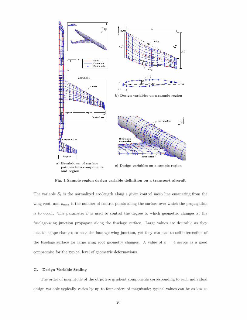
The surface patches are grouped into ‘regions’, with regions being grouped to form ‘components’.
This subdivision is shown in Fig. 1a) for a sample transport aircraft. The design variables of each
region are defined in a coordinate system local to that region. This allows for better control of
local parameters, such as airfoil sections, while global geometric changes occur, such as dihedral.
Figure 1b) shows a sample region and some of the variables which control the shape within the
local coordinate system. These variables allow for the definition and control of planform and section
parameters. The variables shown in Fig. 1b) are non-intuitive to the user, who is primarily concerned
with parameters such as taper, sweep, twist, etc. Instead of using these intuitive parameters as design
variables directly, the non-intuitive set of Fig. 1b) is used, as this allows for as many constraints
as possible to be expressed as linear constraints, which SNOPT can satisfy exactly at the start of
the optimization. These non-intuitive RDVs are coupled through a series of relations to provide
18

intuitive parameters, such that the designer can specify intuitive parameters and their bounds, and
the expression of these in terms of regions variables is transparent to the user.
The RDVs in each region, R, define the control point coordinates of that region in the local
space (XR), and these are transformed to the corresponding control point locations in global space
(X) via the transform
X =
R−1∑
r=1
xtip
LE
b cos Γ
b sin Γ
r
+ φx(ΓR) XR
where Γ is the dihedral angle of each region, and φx is the rotation matrix about the global stream-
wise axis.
For full aircraft configurations, two additional geometric control features are required. The first
is the definition and control of distinct features which are to be designed, such as the wing and
tail of the transport aircraft in Fig. 1a). This introduces the concept of ‘components’, which are
simply groupings of regions which form topologically distinct geometric entities. Global translation
and rotation variables are associated with each component, such that changes in location and pitch
of the wing and tail are handled. The second geometric control feature is a method for handling
the interaction of free and fixed surfaces, such as a wing and fuselage, during the optimization.
Currently, no design variables are associated with the fuselage surface, and the fuselage surface is
driven by geometric changes made to the wing surface. Changes at the wing root are propagated
along the fuselage surface via the relation
xk = x0k + (x1 − x0
1)
[
1 + cos(πSk)
2
]β
for k = 2 . . . kmax
where x is the 3-vector of control point coordinates, and k is the control point index along control
mesh grid lines emanating from the component root as shown in Fig. 1c). The case of k = 1
corresponds to the control points at the fuselage-wing junction that are controlled by design variables
on the wing region. The ‘0’ superscript corresponds to the geometry at the start of the optimization.
19
a) Breakdown of surfacepatches into componentsand region
b) Design variables on a sample region
c) Design variables on a sample region
Fig. 1 Sample region design variable definition on a transport aircraft
The variable Sk is the normalized arc-length along a given control mesh line emanating from the
wing root, and kmax is the number of control points along the surface over which the propagation
is to occur. The parameter β is used to control the degree to which geometric changes at the
fuselage-wing junction propagate along the fuselage surface. Large values are desirable as they
localize shape changes to near the fuselage-wing junction, yet they can lead to self-intersection of
the fuselage surface for large wing root geometry changes. A value of β = 4 serves as a good
compromise for the typical level of geometric deformations.
G. Design Variable Scaling
The order of magnitude of the objective gradient components corresponding to each individual
design variable typically varies by up to four orders of magnitude; typical values can be as low as
20

10−5 and can be as high as 100. It has been found that using design variable scaling can improve
convergence [68], particularly in cases with large numbers of geometric design variables, such as a
case that allows the z-coordinates of the B-spline control points to vary. If a gradient component
is very small and close to the convergence tolerance, the optimizer will focus on varying the control
points with higher gradient components in order to reduce the total gradient.
There are three groups of design variables, each of which can be scaled by a different factor. The
subset of B-spline control point coordinates which are free to move, referred to as geometric design
variables, are typically scaled by a factor of 100.0. Planform design variables are scaled by a factor of
5.0. The angle of attack design variable is not typically scaled. The choice of design variable scaling
can have a significant effect on optimization convergence [68] and is difficult to analyze. Hence it is
suggested that more work be done in this area. The present choices are based on a limited amount
of experimentation, and it is not to be inferred that they are in any sense optimal.
H. Spanwise Lift Distribution Constraint
The substantial computational expense associated with high-fidelity aerostructural optimization
and the current-era scarcity of algorithms with this capability motivates an alternative approach to
wing design that addresses both aerodynamic and structural requirements and can be implemented
in an algorithm with only aerodynamic shape optimization capability. In the optimization case
presented in Section VD a prescribed spanwise lift distribution on the wing of an aircraft is enforced
to ensure that the optimal wing design is feasible with respect to structural considerations. The
prescribed lift distribution may be obtained from a less expensive design tool such as a medium-
fidelity aerostructural optimization algorithm. In the absence of a lift-distribution constraint an
aerodynamic shape optimization can be expected to produce an elliptical lift-distribution that is
not optimal once wing weight is taken into consideration.
A prescribed lift distribution can be enforced by subjecting an aerodynamic shape optimization
to a constraint function given by
C (X) =n∑
i=1
[L∗(yi)− L (X, yi)]2 = 0 (20)
21

where the prescribed lift distribution is represented by a discrete set of target sectional lift values
L∗(yi) defined over a range of spanwise locations given by yi. Sectional lift values at the current
design iteration are given by L (X, yi), where X represents a set of geometric and local angle-of-
attack design variables. In practice the spanwise locations yi used in the constraint function are
coincident with the spanwise locations of geometric design variables that control section shapes.
I. Optimization Convergence Criteria
A successful optimization using SNOPT will satisfy the KKT conditions to within a certain
tolerance. The nonlinear constraints must be satisfied to a user-specifed tolerance such that
‖c‖∞
‖v‖2≤ ε, (21)
where c represents the constraint equations, and v are the scaled design variables. The tolerance
parameter ε is typically set to 1× 10⁻⁶ for the cases presented in this work.
The gradient of the Lagrangian function must also be sufficiently small, satisfying
‖g‖∞
‖ϕ‖2≤ ε, (22)
where g represents the gradient, and ϕ are the adjoint variables within SNOPT’s internal La-
grangian merit function. The tolerance ε for the gradient is typically 1 × 10⁻⁵; however, this level
of convergence is often not achieved.
V. Results
Results are presented in this section which demonstrate the performance of the optimization
methodology in a variety of conditions. A study of the Common Research Model (CRM) wing
geometry in turbulent transonic flow conditions presents optimizations typical of the detailed design
phase and seeks incremental improvements to a given initial geometry such that drag is minimized
at a target lift coefficient. A single-point drag minimization is presented for a blended wing-body
configuration at cruise conditions in order to demonstrate the performance of the methodology when
22

XY
Z
Fig. 2 Blunt trailing-edge CRM wing geometry
considering unconventional geometries.
A. Common Research Model Wing Geometry
A lift-constrained drag minimization is undertaken for the Common Research Model (CRM)
wing-only geometry, shown in Fig. 2, which was obtained from the full wing-body configuration
studied at the Fourth and Fifth Drag Prediction Workshops [69, 70]. This wing features a blunt
trailing edge. The wing-only geometry was obtained by starting with the full wing-body configu-
ration and deleting the fuselage. This leaves the wing root a distance of 120.52 inches from the
original symmetry plane. The leading edge of the wing root is then translated to the origin and
all grid coordinates are scaled by the mean aerodynamic chord (MAC), which has a value of 275.8
inches. At this stage, the entire root chord does not lie exactly on the symmetry plane; additionally,
grid generation can also introduce non-zero symmetry plane coordinates. Consequently, after the
computational mesh is generated using ICEM [71], a post-processing script is applied to all nodes
on the symmetry plane to ensure that they are at y = 0.
The O-O topology computational mesh used for parameterization and mesh movement is made
up of 18 blocks and 3.38 million nodes. Flow analysis is performed on a mesh that is created by
splitting each block of the parameterization mesh into 8 sub-blocks, resulting in a 144-block, 3.57
23

million-node mesh. The MAC is used as the reference length. Applying the grid redistribution
technique produces an off-wall spacing of 2.56 × 10⁻⁶ reference units, resulting in an average y+
value of 1.0 at the first node off of the surface.
The wing geometry has 9 surface patches: 2 each on the upper and lower surfaces, 2 each along
the leading edge and blunt trailing edge, and one cap patch at the wing tip. The leading-edge
patches (one for the inboard section and one for the outboard) are required in order to match with
the blunt trailing-edge patches, and also serve as a method of better capturing the curvature of the
leading edge. Each surface patch is parameterized with 7 control points in the chordwise direction
and 5 in the spanwise direction, with the exception of the patches along the leading and trailing
edges, which have 5 control points in the chordwise direction. The control points at the trailing
edge are fixed, as is the control point at the leading-edge root, while the remaining control points
are allowed to move vertically. Along with the angle of attack, this results in 150 design variables.
For comparison, two additional wings are included in this study. The first is the CRM wing
geometry with a sharp trailing edge, as opposed to a blunt trailing edge, which allows for a compar-
ison between an Euler-based optimization and a RANS-based optimization (the flow near a blunt
trailing edge is unsuited to the inviscid approximation). The second wing has the same planform
as the CRM wing, but is given NACA0012 sections (with a sharp trailing edge) rather than the
section shapes of the original CRM geometry. In order to obtain the sharp trailing edge, a B-spline
representation of the original CRM wing geometry is obtained from the IGES file and modified using
an external script. The B-spline control points are linearly tapered at each spanwise station over the
last 10% of the chord to create a sharp trailing edge located at the average z-coordinate between the
upper and lower edges of the original blunt trailing edge. This alteration to the geometry requires a
different blocking structure in the computational mesh compared to that of the blunt trailing-edge
geometry, as an O-O topology is not feasible with the introduction of the sharp trailing edge. The
two additional geometries consequently use a C-H topology mesh which is made up of 10 surface
patches; the upper surface, lower surface, and cap each have two patches. The inboard and outboard
sections of the leading edge now also have two patches each. The leading-edge and cap patches are
parameterized with 5 control points in the chordwise direction and 5 in the spanwise direction, while
24
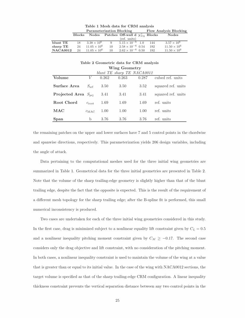
Table 1 Mesh data for CRM analysis
Parameterization Blocking Flow Analysis Blocking
Blocks Nodes Patches Off-wall d y+avg Blocks Nodes
(ref. units)blunt TE 18 3.38× 10
6 9 5.15× 10⁻⁶ 1.0 144 3.57× 10
6
sharp TE 24 11.05× 10⁶ 10 2.58× 10⁻⁶ 0.54 192 11.50× 10⁶
NACA0012 24 11.05× 10⁶ 10 2.62× 10⁻⁶ 0.50 192 11.50× 10⁶
Table 2 Geometric data for CRM analysis
Wing Geometryblunt TE sharp TE NACA0012
Volume V 0.262 0.263 0.287 cubed ref. units
Surface Area Ssrf 3.50 3.50 3.52 squared ref. units
Projected Area Sprj 3.41 3.41 3.41 squared ref. units
Root Chord croot 1.69 1.69 1.69 ref. units
MAC cMAC 1.00 1.00 1.00 ref. units
Span b 3.76 3.76 3.76 ref. units
the remaining patches on the upper and lower surfaces have 7 and 5 control points in the chordwise
and spanwise directions, respectively. This parameterization yields 206 design variables, including
the angle of attack.
Data pertaining to the computational meshes used for the three initial wing geometries are
summarized in Table 1. Geometrical data for the three initial geometries are presented in Table 2.
Note that the volume of the sharp trailing-edge geometry is slightly higher than that of the blunt
trailing edge, despite the fact that the opposite is expected. This is the result of the requirement of
a different mesh topology for the sharp trailing edge; after the B-spline fit is performed, this small
numerical inconsistency is produced.
Two cases are undertaken for each of the three initial wing geometries considered in this study.
In the first case, drag is minimized subject to a nonlinear equality lift constraint given by CL = 0.5
and a nonlinear inequality pitching moment constraint given by CM ≥ −0.17. The second case
considers only the drag objective and lift constraint, with no consideration of the pitching moment.
In both cases, a nonlinear inequality constraint is used to maintain the volume of the wing at a value
that is greater than or equal to its initial value. In the case of the wing with NACA0012 sections, the
target volume is specified as that of the sharp trailing-edge CRM configuration. A linear inequality
thickness constraint prevents the vertical separation distance between any two control points in the
25

Table 3 Initial lift, drag, and moment data for CRM analysis
Wing GeometryBlunt TE Sharp TE NACA0012
CL 0.500 0.500 0.500
CD 0.0212 0.0205 0.0681
CM -0.1740 -0.1628 -0.0114
α (◦) 2.32 2.41 5.40
same vertical plane from going below 25% of its initial value.
Case 1 refers to the lift-constrained drag minimization with the nonlinear inequality pitching
moment constraint. Case 2 refers to the optimization run as a lift-constrained drag minimization
problem with no consideration of the pitching moment. Apart from the use of the pitching moment
constraint, the two cases are identical.
Flow analyses are performed at a Mach number of 0.85, a Reynolds number of 5 million (based
on the reference length), and an initial angle of attack of 2.2◦. Pitching moments are taken about the
point (1.2077, 0.0, 0.007669) MAC units relative to an origin located at the leading-edge root. These
conditions and conventions are consistent with those used in the Drag Prediction Workshop analysis.
The lift, drag, and pitching moment coefficients corresponding to the three initial geometries at the
specified Mach and Reynolds numbers are presented in Table 3. The angles of attack have been
adjusted so that each geometry can be compared at the target lift coefficient of CL = 0.5. All
coefficients are calculated using the projected area as the reference area, Sref = Sprj = 3.407 squared
reference units.
The coefficients of lift, drag, and pitching moment are displayed in Table 4 for the three initial
geometries and the corresponding optimization results from Cases 1 and 2. The lift-to-drag ratio
improves by 7-10% in the blunt trailing-edge and sharp trailing-edge cases, while the ratio improved
by over 200% over the initial geometry with NACA0012 sections. In each case, the constraints on lift
and volume are satisfied, as is the pitching moment constraint for the Case 1 results. The geometries
produced in the Case 2 optimizations produce slightly lower drag coefficients compared to the Case
1 geometries and produce larger nose-down positive pitching moment coefficients. Convergence
histories for the three initial geometries are presented in Figs. 3, 4, and 5. In these plots, feasibility
26

Table 4 Lift, drag, and moment data for CRM wing optimizations
Blunt TE Sharp TE NACA0012Initial Case 1 Case 2 Initial Case 1 Case 2 Initial Case 1 Case 2
CL 0.500 0.500 0.500 0.500 0.500 0.500 0.500 0.500 0.500
CD 0.0212 0.0193 0.0192 0.0205 0.0191 0.0189 0.0681 0.0190 0.0189
CL
CD23.6 25.9 26.0 24.4 26.2 26.5 7.34 26.3 26.4
CM -0.1740 -0.1700 -0.2090 -0.1628 -0.1699 -0.1927 -0.0114 -0.1695 -0.1994
α (◦) 2.32 2.70 1.93 2.41 2.48 2.28 5.40 2.49 2.01
function evaluations
feas
ibili
ty
0 20 40 60 80 100
10-6
10-5
10-4
CM & CL constraints (Case 1)CL constraint (Case 2)
a) feasibility
function evaluations
optim
ality
0 50 100
10-4
10-3
CM & CL constraints (Case 1)CL constraint (Case 2)
b) optimality
function evaluations
mer
it fu
nctio
n
0 20 40 60 80
0.066
0.068
0.070
0.072
0.074
CM & CL constraints (Case 1)CL constraint (Case 2)
c) merit function
Fig. 3 Convergence histories of blunt trailing-edge CRM cases
represents the ability of the optimizer to meet the nonlinear constraints, optimality is a measure of
the gradient of SNOPT’s Lagrangian merit function, and the merit function represents the objective
function and any nonlinear constraint violations. In each case, the feasibility is improved by at least
two orders of magnitude. Optimality is reduced by a maximum of one order of magnitude; deeper
convergence is difficult to achieve without either reducing the number of design variables or imposing
tighter constraints on them.
Contour plots of the coefficient of pressure are presented for the initial and optimized results
from all three initial geometries in Figs. 6, 7, and 8. In the case of the wing with the blunt trailing
edge, the results of Cases 1 and 2 have done a good job of removing the shocks present on the
surface of the initial geometry. A spike in the coefficient of pressure is present near the leading edge
of the initial geometry; this is caused by the fitting of the computational mesh, which is not able
to perfectly capture the curvature of the leading edge. However, it is interesting to note that the
optimizer is able to reduce this effect. The results of the optimizations of the sharp trailing-edge
configuration and the geometry with NACA0012 sections are shock-free.
27

function evaluations
feas
ibili
ty
5 10 15 20 2510-7
10-6
10-5
10-4
CL & CM constraints (Case 1)CL constraint (Case 2)
a) feasibility
function evaluations
optim
ality
0 10 20 30 40
10-4
10-3
CL & CM constraints (Case 1)CL constraint (Case 2)
b) optimality
function evaluations
mer
it fu
nctio
n
5 10 15 20 25
0.064
0.065
0.065
0.066
0.066
0.067
CL & CM constraints (Case 1)CL constraint (Case 2)
c) merit function
Fig. 4 Convergence histories of sharp trailing-edge CRM cases
function evaluations
feas
ibili
ty
0 20 40 60 80 100
10-7
10-6
10-5
10-4
10-3
CL & CM constraints (Case 1)CL constraint (Case 2)
a) feasibility
function evaluations
optim
ality
0 20 40 60 80 100
10-4
10-3
10-2
CL & CM constraints (Case 1)CL constraint (Case 2)
b) optimality
function evaluations
mer
it fu
nctio
n
0 20 40 60 80 100
0.040
0.045
0.050
0.055
0.060
0.065
0.070
0.075
CL & CM constraints (Case 1)CL constraint (Case 2)
c) merit function
Fig. 5 Convergence histories of NACA0012 CRM cases
The spanwise lift distributions of the initial geometry and the results of Cases 1 and 2 are com-
pared to an elliptical distribution in Fig. 9 for each of the geometries considered. The optimized
blunt trailing-edge cases show distributions much closer to elliptical than the distribution corre-
sponding to the initial geometry. In the case of the sharp trailing edge, Case 2 was able to achieve
a near-elliptical distribution, while the distribution resulting from Case 1 was not, although there
is visible improvement compared to the initial geometry. For the initial geometry with NACA0012
sections, Case 2 is able to achieve a nearly elliptical distribution. Maintaining the pitching mo-
ment constraint in Case 1, however, may be preventing the optimizer from achieving the tip loading
necessary to produce an overall elliptical distribution.
The optimization of the wing with NACA0012 sections applied to the initial CRM wing planform
produces similar drag data at the target lift to those initialized with blunt and sharp trailing-edge
CRM wing geometries, even though the optimizer appears to produce a different shape for each
of the three geometries, particularly for the moment-constrained cases. The section geometries are
28

X
Y
Z
Cp
10.70.40.1
-0.2-0.5-0.8-1.1
Flow direction
a) Initial geometry
X
Y
Z
Cp
10.70.40.1
-0.2-0.5-0.8-1.1
Flow direction
b) CL and CM constraints
X
Y
Z
Cp
10.70.40.1
-0.2-0.5-0.8-1.1
Flow direction
c) CL constraint
Fig. 6 Surface pressure coefficient contours on the upper surface for the blunt trailing-edgeCRM cases
X
Y
Z
Cp
10.70.40.1
-0.2-0.5-0.8-1.1
Flow direction
a) Initial geometry
X
Y
Z
Cp
10.70.40.1
-0.2-0.5-0.8-1.1
Flow direction
b) CL and CM constraints
X
Y
Z
Cp
10.70.40.1
-0.2-0.5-0.8-1.1
Flow direction
c) CL constraintn
Fig. 7 Surface pressure coefficient contours on the upper surface for the sharp trailing-edgeCRM cases
compared for the cases using the lift and pitching moment constraints in Fig. 10 and for the cases
with no moment constraint in Fig. 11. With the exception of the 2.35% span location, the blunt
and sharp trailing-edge geometries appear to be producing similar results at the inboard sections.
As the sections are observed further outboard, however, there is more similarity between the sharp
trailing-edge and NACA0012-sectioned geometries. The fact that the NACA0012-sectioned wing
was able to achieve the same lift and drag as the two CRM wings, despite starting from a very
different initial geometry, while also producing a final geometry that differs substantially from the
results of the sharp and blunt trailing-edge CRM wings, suggests that the design space for this
problem is either multi-modal or contains a flat valley.
For the blunt trailing edge case shown in Fig. 10, the final geometry contains a sharp feature
at the leading edge that is most noticeable near the wing tip. This feature is likely the result of
the high degree of geometric flexibility at the leading edge, which the optimizer exploits to improve
the load distribution while satisfying the pitching moment constraint. This effect is reduced when
29

X
Y
Z
Cp
10.70.40.1
-0.2-0.5-0.8-1.1
Flow direction
a) Initial geometry
X
Y
Z
Cp
10.70.40.1
-0.2-0.5-0.8-1.1
Flow direction
b) CL and CM constraints
X
Y
Z
Cp
10.70.40.1
-0.2-0.5-0.8-1.1
Flow direction
c) CL constraint
Fig. 8 Surface pressure coefficient contours on the upper surface for the NACA0012 CRMcases
Y
Lift
0 0.5 1 1.5 2 2.5 3 3.5
0
0.1
0.2
0.3
0.4
0.5
0.6
Elliptical distributionInitial geometryCL & CM constrained resultCL constrained result
a) Blunt TE
Y
Lift
0 1 2 30
0.1
0.2
0.3
0.4
0.5
0.6
Elliptical distributionInitial geometryCL & CM constrained resultCL constrained result
b) Sharp TE
Y
Lift
0 0.5 1 1.5 2 2.5 3 3.50
0.1
0.2
0.3
0.4
0.5
0.6
0.7
0.8
0.9
Elliptical distributionInitial geometryLift and moment constrained resultLift constrained result
c) NACA0012
Fig. 9 Lift distribution comparison for CRM wing optimizations
multiple operating conditions are considered, and could be eliminated if dive constraints are used
[14]. Introducing additional constraints limiting the geometric flexibility near the leading edge
could also prevent this. Moreover, the optimized wings have thinner outboard sections with thicker
sections near the wing root relative to the original CRM geometry. We emphasize that this is a test
problem to characterize the performance of an aerodynamic shape optimization methodology, not
a practical wing design study. A high degree of geometric flexibility has been permitted in order to
provide a stiff test of the optimization methodology.
To obtain a better understanding of the nature of the design space for the CRM study, several
different sets of perturbations were applied to the CRM planform wing with NACA0012 sections
initially. The drag minimization with constrained lift and pitching moment was run for each of
the new initial geometries. To create the modified geometries, the sharp trailing-edge CRM wing
geometry is used initially; the z-coordinates of the CRM planform wing with NACA0012 sections
are then applied to isolated sections of the initial geometry, creating a family of initial designs. The
30

X/c
Z/c
0 0.2 0.4 0.6 0.8 1-0.12
-0.1
-0.08
-0.06
-0.04
-0.02
0
0.02
0.04
blunt TE moment constraintsharp TE moment constraintNACA0012 moment constraint
a) 2.35% span
X/c
Z/c
0 0.2 0.4 0.6 0.8 1
-0.04
-0.02
0
0.02
0.04
0.06
blunt TE moment constraintsharp TE moment constraintNACA0012 moment constraint
b) 26.7% span
X/c
Z/c
0 0.2 0.4 0.6 0.8 10.06
0.08
0.1
0.12
0.14
0.16
blunt TE moment constraintsharp TE moment constraintNACA0012 moment constraint
c) 55.7% span
X/c
Z/c
0 0.2 0.4 0.6 0.8 1
0.18
0.2
0.22
0.24
0.26
0.28
blunt TE moment constraintsharp TE moment constraintNACA0012 moment constraint
d) 69.5% span
X/c
Z/c
0 0.2 0.4 0.6 0.8 1
0.36
0.38
0.4
0.42
0.44
0.46
blunt TE moment constraintsharp TE moment constraintNACA0012 moment constraint
e) 82.8% span
X/c
Z/c
0 0.2 0.4 0.6 0.8 1
0.62
0.64
0.66
0.68
0.7
0.72
blunt TE moment constraintsharp TE moment constraintNACA0012 moment constraint
f) 94.4% span
Fig. 10 Section shape comparison for three CRM wing geometries, drag objective with liftand moment constraints
X/c
Z/c
0 0.2 0.4 0.6 0.8 1-0.12
-0.1
-0.08
-0.06
-0.04
-0.02
0
0.02
0.04
blunt TE dragsharp TE dragNACA0012 drag
a) 2.35% span
X/c
Z/c
0 0.2 0.4 0.6 0.8 1
-0.04
-0.02
0
0.02
0.04
0.06
blunt TE dragsharp TE dragNACA0012 drag
b) 26.7% span
X/c
Z/c
0 0.2 0.4 0.6 0.8 10.06
0.08
0.1
0.12
0.14
0.16
blunt TE dragsharp TE dragNACA0012 drag
c) 55.7% span
X/c
Z/c
0 0.2 0.4 0.6 0.8 1
0.18
0.2
0.22
0.24
0.26
0.28
blunt TE dragsharp TE dragNACA0012 drag
d) 69.5% span
X/c
Z/c
0 0.2 0.4 0.6 0.8 1
0.36
0.38
0.4
0.42
0.44
0.46
blunt TE dragsharp TE dragNACA0012 drag
e) 82.8% span
X/c
Z/c
0 0.2 0.4 0.6 0.8 10.62
0.64
0.66
0.68
0.7
0.72
blunt TE dragsharp TE dragNACA0012 drag
f) 94.4% span
Fig. 11 Section shape comparison for three CRM wing geometries, drag objective with liftconstraint
31

Table 5 Summary of initial geometries for CRM wing design space investigation
Initial Design # NACA0012 Data Applied To:
1 Inboard patches only
2 Outboard patches only
3 Upper surface patches only
4 Lower surface patches only
5 Upper inboard patches only
6 Lower inboard patches only
7 Upper outboard patches only
8 Lower outboard patches only
Table 6 Coefficient data from design space study of CRM wing with sharp trailing edge
Initial Design # CL CD CM
1 0.500 0.0189 -0.1698
2 0.500 0.0189 -0.1700
3 0.500 0.0190 -0.1698
4 0.500 0.0191 -0.1699
5 0.497 0.0188 -0.1685
6 0.500 0.0190 -0.1699
7 0.500 0.0189 -0.1700
8 0.500 0.0189 -0.1698
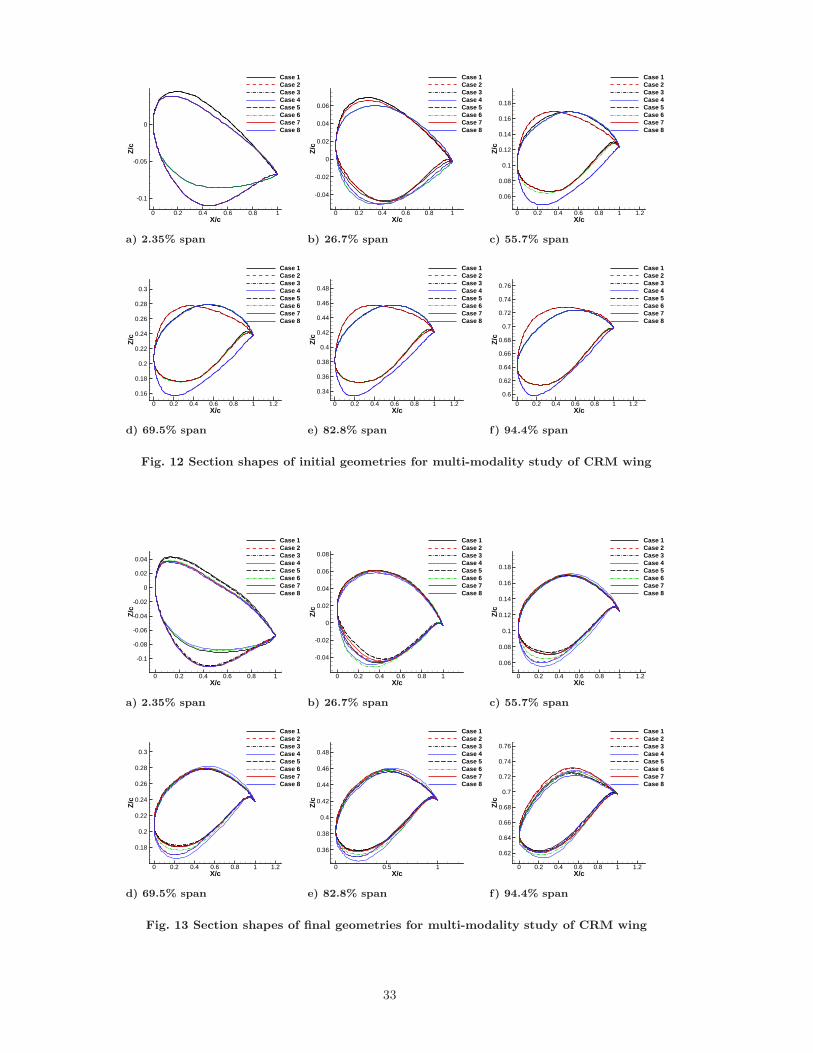
initial designs are summarized in Table 5, which lists the regions of the initial geometry to which
the NACA0012 data are applied. The section shapes of the set of initial geometries are shown in
Fig. 12. The optimizer achieved at least one order reduction in optimality in each case. Despite
the comparison of the eight final geometries in Fig. 13 showing that the optimizer produces visibly
different results for the different initial geometries, each of the results exhibits comparable drag and
pitching moment coefficients at the target lift coefficient, as shown in Table 6. This indicates that
the design space for this problem is relatively flat and provides an explanation as to why the sharp
trailing-edge CRM wing and the CRM planform wing with NACA0012 sections produced different
geometries. However, the possibility of a multi-modal design space cannot be completely discounted;
deeper convergence of the optimizer would allow for a more definitive conclusion as to whether the
design space contains a flat valley or is multi-modal.
32
X/c
Z/c
0 0.2 0.4 0.6 0.8 1
-0.1
-0.05
0
Case 1Case 2Case 3Case 4Case 5Case 6Case 7Case 8
a) 2.35% span
X/c
Z/c
0 0.2 0.4 0.6 0.8 1
-0.04
-0.02
0
0.02
0.04
0.06
Case 1Case 2Case 3Case 4Case 5Case 6Case 7Case 8
b) 26.7% span
X/c
Z/c
0 0.2 0.4 0.6 0.8 1 1.2
0.06
0.08
0.1
0.12
0.14
0.16
0.18
Case 1Case 2Case 3Case 4Case 5Case 6Case 7Case 8
c) 55.7% span
X/c
Z/c
0 0.2 0.4 0.6 0.8 1 1.2
0.16
0.18
0.2
0.22
0.24
0.26
0.28
0.3
Case 1Case 2Case 3Case 4Case 5Case 6Case 7Case 8
d) 69.5% span
X/c
Z/c
0 0.2 0.4 0.6 0.8 1 1.2
0.34
0.36
0.38
0.4
0.42
0.44
0.46
0.48
Case 1Case 2Case 3Case 4Case 5Case 6Case 7Case 8
e) 82.8% span
X/c
Z/c
0 0.2 0.4 0.6 0.8 1 1.2
0.6
0.62
0.64
0.66
0.68
0.7
0.72
0.74
0.76
Case 1Case 2Case 3Case 4Case 5Case 6Case 7Case 8
f) 94.4% span
Fig. 12 Section shapes of initial geometries for multi-modality study of CRM wing
X/c
Z/c
0 0.2 0.4 0.6 0.8 1
-0.1
-0.08
-0.06
-0.04
-0.02
0
0.02
0.04
Case 1Case 2Case 3Case 4Case 5Case 6Case 7Case 8
a) 2.35% span
X/c
Z/c
0 0.2 0.4 0.6 0.8 1
-0.04
-0.02
0
0.02
0.04
0.06
0.08
Case 1Case 2Case 3Case 4Case 5Case 6Case 7Case 8
b) 26.7% span
X/c
Z/c
0 0.2 0.4 0.6 0.8 1 1.2
0.06
0.08
0.1
0.12
0.14
0.16
0.18
Case 1Case 2Case 3Case 4Case 5Case 6Case 7Case 8
c) 55.7% span
X/c
Z/c
0 0.2 0.4 0.6 0.8 1 1.2
0.18
0.2
0.22
0.24
0.26
0.28
0.3
Case 1Case 2Case 3Case 4Case 5Case 6Case 7Case 8
d) 69.5% span
X/c
Z/c
0 0.5 1
0.36
0.38
0.4
0.42
0.44
0.46
0.48
Case 1Case 2Case 3Case 4Case 5Case 6Case 7Case 8
e) 82.8% span
X/c
Z/c
0 0.2 0.4 0.6 0.8 1 1.2
0.62
0.64
0.66
0.68
0.7
0.72
0.74
0.76
Case 1Case 2Case 3Case 4Case 5Case 6Case 7Case 8
f) 94.4% span
Fig. 13 Section shapes of final geometries for multi-modality study of CRM wing
33

Table 7 Coefficients for CRM wing with blunt trailing edge on optimization mesh and finemesh
Initial Geometry Optimized GeometryMesh Size (nodes) 3.4× 10⁶ 39.8× 10⁶ 3.4× 10⁶ 39.8× 10⁶
CL 0.500 0.500 0.500 0.500
CD 0.0212 0.0197 0.0193 0.0186
CM -0.1740 -0.1862 -0.1700 -0.1730
Table 8 Coefficients for CRM wing with sharp trailing edge on optimization mesh and finemesh
Initial Geometry Optimized GeometryMesh Size (nodes) 11.0× 10⁶ 35.5× 10⁶ 11.0× 10⁶ 35.5× 10⁶
CL 0.500 0.500 0.500 0.500
CD 0.0205 0.0203 0.0191 0.0188
CM -0.1628 -0.1640 -0.1699 -0.1711
To ensure that the improvement in the drag coefficient carries over to a very fine grid level, the
initial and optimized geometries were evaluated on meshes made up of over 35 million nodes in Tables
7, 8, and 9. The coefficients obtained on the fine mesh are compared to those obtained from the mesh
used in the optimization with lift and pitching moment constraints. At the target lift coefficient,
the largest discrepancy is in the drag coefficient for the initial blunt trailing-edge geometry, which
exhibits a difference of 7.6% relative to the drag coefficient on the fine mesh. The pitching moment
coefficient differs by 6.6% relative to the fine mesh. For the optimized blunt trailing-edge geometry,
the drag coefficient and pitching moment coefficient differ by 3.8% and 0.02%, respectively, between
the mesh used in the optimization and the fine mesh. A 5.6% relative improvement in drag is
demonstrated on the fine mesh between the initial and final geometries. This demonstrates that
the geometry produced by the optimizer significantly reduces the objective function relative to the
original geometry, even on a finer mesh than that used for the optimization. Good agreement in the
lift and pitching moment coefficients is also demonstrated between the coarser and fine meshes for
the sharp trailing-edge and NACA0012 configurations. However, if strict satisfaction of a constraint
such as the pitching moment is desired, then a finer mesh should be used for the optimization.
34

Table 9 Coefficients for CRM wing with NACA0012 sections on optimization mesh and finemesh
Initial Geometry Optimized GeometryMesh Size (nodes) 11.0× 10⁶ 35.5× 10⁶ 11.0× 10⁶ 35.5× 10⁶
CL 0.500 0.500 0.500 0.500
CD 0.0681 0.0611 0.0191 0.0190
CM -0.0114 -0.0400 -0.1700 -0.1699
B. Optimization with Section Shape and Planform Design Variables
Since structures are not considered in the cases presented in this paper, the wing planform
shapes are typically fixed. However, the aerodynamic shape optimization algorithm will eventually
be incorporated with a structural solver so that aerostructural optimization can be performed.
Consequently, it is important to ensure that the aerodynamic optimization algorithm is capable of
accommodating large planform changes as well as section shape changes. Here we present such an
optimization problem. It is intended solely to demonstrate the ability of the methodology to handle
large geometric changes such as can be encountered in an aerostructural optimization; it is not a
practical example.
The initial geometry is a rectangular wing initially fit with NACA0012 sections. The root
chord is used as the reference length. The initial wing has a semi-span of 2.0 reference units and
a projected area of 2.0 squared reference units. The computational mesh is made up of 12 blocks
and 8.46 million nodes; each block of the mesh is parameterized with a 9 × 9 × 9 B-spline control
volume. Flow analysis is performed on a 96-block equivalent mesh that is obtained by subdividing
each block of the 12-block mesh into 8 blocks. The parameter extraction method is used to obtain
an average off-wall spacing of 2.53× 10⁻⁶ reference units, resulting in an average y+ value of 0.4.
The z-coordinates of the B-spline control points on the aerodynamic surface are used as section
and twist variables, along with the angle of attack. The trailing-edge control points are fixed.
Additionally, the leading-edge and trailing-edge sweep angles are allowed to vary, creating taper.
The span can also increase. In total, this problem has 131 design variables. A minimum volume
constraint is enforced based on the initial geometry. The sweep angles have an upper bound of 45.0◦,
while the semi-span has an upper bound of 5.0 reference units. We reiterate that the geometries
produced in this study are not meant to represent practical aerodynamic configurations; rather, the
35

function evaluations
feas
ibili
ty
0 20 40 60 80
10-5
10-4
10-3
10-2
a) Feasibility
function evaluations
optim
ality
0 20 40 60 8010-3
10-2
10-1
100
b) Optimality
function evaluations
mer
it fu
nctio
n
0 20 40 60 80
0.06
0.08
0.1
0.12
0.14
0.16
c) Merit function
Fig. 14 Convergence history for optimization of rectangular wing in transonic flow
purpose of this study is to demonstrate the geometric flexibility and robustness of the presented
methodology in the presence of large shape changes.
The objective of this design problem is to minimize drag at a Mach number of 0.84 and a
Reynolds number of 5 million, subject to a lift constraint, where the constrained lift quantity is
defined as the product of the lift coefficient and the reference area, CL ∗ Sref . The projected area is
used as the reference area. Note that the initial geometry cannot satisfy the CL ∗ Sref constraint.
Convergence data are presented in Fig. 14, where, after 120 hours on 108 processors, a reduction
of between one and two orders of magnitude is observed in the optimality. The spikes in the
convergence plots show where the optimizer must work to minimize the lift constraint penalty; after
the lift approaches the target, the merit function decreases and eventually levels off. The lift and
drag data corresponding to the initial and optimized geometries are compared in Table 10, where
the coefficients corresponding to the initial geometry are obtained using the initial projected area
of 2.0 squared reference units as the reference area, and the coefficients for the final geometry use
the projected area of the final geometry, Sref = 3.7 squared reference units. The data show that the
lift-to-drag ratio has improved by a factor of four.
The changes in the planform variables are illustrated in Fig. 15, which shows a three-dimensional
view of the initial and final surface geometries, with the positions of the B-spline control points
represented as spheres. The wing is swept back and the span is increased by approximately 60% to
3.2 reference units. The minimum volume constraint is not active for the final geometry. The final
leading-edge and trailing-edge sweep angles are 25.6◦ and 29.8◦, respectively; neither angle reached
36

Table 10 Lift, drag, and moment data for optimization of rectangular wing in transonic flow
Initial geometry Optimized geometryCL ∗ Sref 0.2888 0.9650
CL 0.1444 0.2594
CD ∗ Sref 0.0561 0.0472
CD 0.0280 0.0127
CL/CD 5.1 20.4
X
Y
ZInitial geometryOptimized geometry
Fig. 15 3D comparison of geometries from optimization of rectangular wing in transonic flow
its upper bound of 45.0◦, nor did the span reach its upper bound of 5.0 reference units. Section
geometries at three spanwise stations, along with corresponding plots of coefficient of pressure, are
presented in Figs. 16 and 17, respectively. Span percentages are specified relative to the initial
geometry so that the locations of the sections (i.e. the y-coordinates corresponding to each spanwise
section) remain consistent between the initial and optimized geometries. Additionally, noting the
varying chord lengths along the span, the leading-edge coordinates are aligned in the images in
order to facilitate a visual comparison. The coefficient of pressure data are obtained for the initial
geometry at the initial lift coefficient of CL = 0.1444 (where Sref = 2.0 squared reference units)
and the optimized geometry at the final lift coefficient, CL = 0.2594 (Sref = 3.72 squared reference
units). The final geometry comprises thinner section shapes with a cambered trailing-edge, and the
optimizer has significantly reduced the strength of the shock, although it was not able to eliminate
37

X/c
Z/c
0 0.2 0.4 0.6 0.8 1
-0.06
-0.04
-0.02
0
0.02
0.04
0.06
Initial geometry, 2% span 0
Optimized geometry, 2% span 0
a)
X/c
Z/c
0 0.2 0.4 0.6 0.8 1-0.06
-0.04
-0.02
0
0.02
0.04
0.06
Initial geometry, 65% span 0
Optimized geometry, 65% span 0
b)
X/c
Z/c
0 0.2 0.4 0.6 0.8 1-0.06
-0.04
-0.02
0
0.02
0.04
0.06
Initial geometry, 90% span 0
Optimized geometry, 90% span 0
c)
Fig. 16 Section shapes for optimization of rectangular wing in transonic flow
X/c
Cp
0 0.2 0.4 0.6 0.8 1
-1
-0.5
0
0.5
1
Initial geometry, 2% span 0
Optimized geometry, 2% span 0
a)
X/c
Cp
0 0.2 0.4 0.6 0.8 1
-1
-0.5
0
0.5
1
Initial geometry, 65% span 0
Optimized geometry, 65% span 0
b)
X/c
Cp
0 0.2 0.4 0.6 0.8 1
-1
-0.5
0
0.5
1
Initial geometry, 90% span 0
Optimized geometry, 90% span 0
c)
Fig. 17 Surface pressure coefficient data for optimization of rectangular wing in transonic flow
it entirely. The large improvement in lift-to-drag ratio results primarily from the reduction of wave
drag from the near-elimination of shock waves and the induced drag reduction associated with the
span increase.
The initial and final geometries were analyzed on a 30 million-node mesh, and the results are
compared to the data obtained from the optimization on the 8.5 million-node mesh in Table 11.
Although the force coefficients are not fully grid converged, the improvement in the lift-to-drag
ratio is also seen on the fine mesh. Overall, this problem demonstrates the ability of the flow solver
and mesh movement methodology to handle a wide variety of geometries. Thus, the optimization
methodology is capable of addressing problems where large shape changes are encountered.
38

Table 11 Coefficients for rectangular wing on optimization mesh and fine mesh
Initial Geometry Optimized GeometryMesh Size (nodes) 8.5× 10⁶ 30.2× 10⁶ 8.5× 10⁶ 30.2× 10⁶
CL ∗ Sref 0.2888 0.2888 0.9650 0.9650
CL 0.1444 0.1444 0.2594 0.2594
CD ∗ Sref 0.0561 0.0562 0.0472 0.0461
CD 0.0280 0.0281 0.0127 0.0124
CL/CD 5.1 5.1 20.4 20.9
C. Comparison of Optimization Based on the Euler Equations with that Based on the RANS
Equations
Optimization based on inviscid analysis is a popular approach based on its low computational
cost and high degree of robustness compared to viscous analysis. There are certainly situations in
which a designer would be tempted to rely on inviscid analysis, and others in which viscous effects
are too significant to ignore or approximate. For example, optimizations of high-lift, multi-element
configurations, or geometries near their maximum lift, would require viscous analysis. However, in
cases where the flow is fully attached and any shocks present are weak, inviscid analysis can predict
lift and surface pressure distributions relatively accurately. In such cases, particularly within a mul-
tidisciplinary framework where the computational cost and potentially limited robustness associated
with viscous analysis can be prohibitive, inviscid analysis is an attractive option. Approximations
of the viscous drag can be obtained based on surface area.
To investigate the effect of relying on inviscid analysis in aerodynamic shape optimization, the
drag minimization of the sharp trailing-edge CRM wing configuration with lift and pitching moment
constraints presented in Section VA is repeated, this time based on the Euler equations. A RANS
analysis is performed on the resulting geometry at the lift coefficient of CL = 0.50 to compare the
result of the optimization based on the Euler equations to that based on the RANS equations.
The section shapes produced by the Euler and RANS optimizations at six spanwise locations
are presented in Fig. 18, followed by the corresponding distributions of coefficient of pressure based
on a RANS computation in Fig. 19. While the geometry resulting from the RANS optimization is
shock-free, a strong surface shock is present near the mid-chord for the Euler-optimized geometry.
Note that, based on an inviscid analysis, the Euler-optimized geometry is shock-free; the shock arises
39
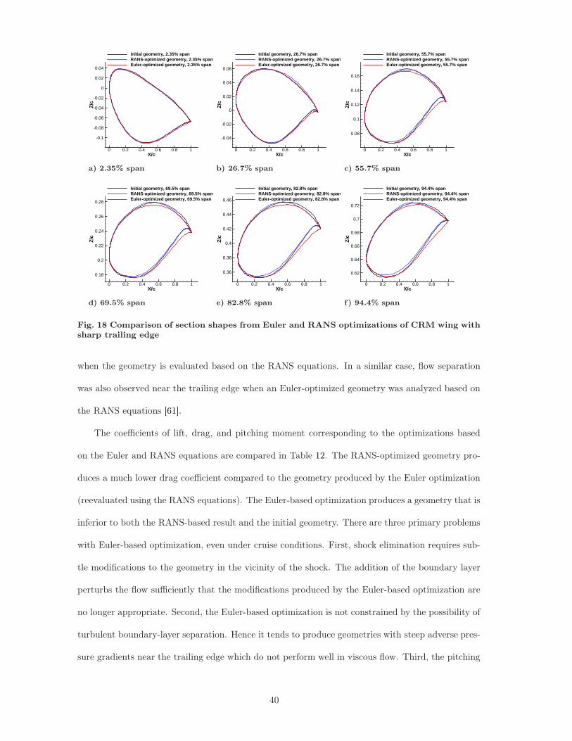
X/c
Z/c
0 0.2 0.4 0.6 0.8 1
-0.1
-0.08
-0.06
-0.04
-0.02
0
0.02
0.04
Initial geometry, 2.35% spanRANS-optimized geometry, 2.35% spanEuler-optimized geometry, 2.35% span
a) 2.35% span
X/c
Z/c
0 0.2 0.4 0.6 0.8 1
-0.04
-0.02
0
0.02
0.04
0.06
Initial geometry, 26.7% spanRANS-optimized geometry, 26.7% spanEuler-optimized geometry, 26.7% span
b) 26.7% span
X/c
Z/c
0 0.2 0.4 0.6 0.8 1
0.08
0.1
0.12
0.14
0.16
Initial geometry, 55.7% spanRANS-optimized geometry, 55.7% spanEuler-optimized geometry, 55.7% span
c) 55.7% span
X/c
Z/c
0 0.2 0.4 0.6 0.8 1
0.18
0.2
0.22
0.24
0.26
0.28
Initial geometry, 69.5% spanRANS-optimized geometry, 69.5% spanEuler-optimized geometry, 69.5% span
d) 69.5% span
X/c
Z/c
0 0.2 0.4 0.6 0.8 1
0.36
0.38
0.4
0.42
0.44
0.46
Initial geometry, 82.8% spanRANS-optimized geometry, 82.8% spanEuler-optimized geometry, 82.8% span
e) 82.8% span
X/c
Z/c
0 0.2 0.4 0.6 0.8 1
0.62
0.64
0.66
0.68
0.7
0.72
Initial geometry, 94.4% spanRANS-optimized geometry, 94.4% spanEuler-optimized geometry, 94.4% span
f) 94.4% span
Fig. 18 Comparison of section shapes from Euler and RANS optimizations of CRM wing withsharp trailing edge
when the geometry is evaluated based on the RANS equations. In a similar case, flow separation
was also observed near the trailing edge when an Euler-optimized geometry was analyzed based on
the RANS equations [61].
The coefficients of lift, drag, and pitching moment corresponding to the optimizations based
on the Euler and RANS equations are compared in Table 12. The RANS-optimized geometry pro-
duces a much lower drag coefficient compared to the geometry produced by the Euler optimization
(reevaluated using the RANS equations). The Euler-based optimization produces a geometry that is
inferior to both the RANS-based result and the initial geometry. There are three primary problems
with Euler-based optimization, even under cruise conditions. First, shock elimination requires sub-
tle modifications to the geometry in the vicinity of the shock. The addition of the boundary layer
perturbs the flow sufficiently that the modifications produced by the Euler-based optimization are
no longer appropriate. Second, the Euler-based optimization is not constrained by the possibility of
turbulent boundary-layer separation. Hence it tends to produce geometries with steep adverse pres-
sure gradients near the trailing edge which do not perform well in viscous flow. Third, the pitching
40

X/c
Cp
0 0.2 0.4 0.6 0.8 1
-0.5
0
0.5
Initial geometry, 2.35% spanRANS-optimized geometry, 2.35% spanEuler-optimized geometry, 2.35% span
a) 2.35% span
X/c
Cp
0 0.2 0.4 0.6 0.8 1
-1
-0.5
0
0.5
Initial geometry, 26.7% spanRANS-optimized geometry, 26.7% spanEuler-optimized geometry, 26.7% span
b) 26.7% span
X/c
Cp
0 0.2 0.4 0.6 0.8 1
-1
-0.5
0
0.5
Initial geometry, 55.7% spanRANS-optimized geometry, 55.7% spanEuler-optimized geometry, 55.7% span
c) 55.7% span
X/c
Cp
0 0.2 0.4 0.6 0.8 1
-1
-0.5
0
0.5
Initial geometry, 69.5% spanRANS-optimized geometry, 69.5% spanEuler-optimized geometry, 69.5% span
d) 69.5% span
X/c
Cp
0 0.2 0.4 0.6 0.8 1
-1
-0.5
0
0.5
Initial geometry, 82.8% spanRANS-optimized geometry, 82.8% spanEuler-optimized geometry, 82.8% span
e) 82.8% span
X/c
Cp
0 0.2 0.4 0.6 0.8 1
-1
-0.5
0
0.5
Initial geometry, 94.4% spanRANS-optimized geometry, 94.4% spanEuler-optimized geometry, 94.4% span
f) 94.4% span
Fig. 19 Comparison of surface pressure coefficient data from Euler and RANS optimizationsof CRM wing with sharp trailing edge (RANS analysis)
Table 12 Force coefficient data from RANS analyses of Euler-based and RANS-based CRMoptimizations with pitching moment constraint
Geometry CL CD CM
Initial 0.500 0.0205 -0.1628
Euler result (RANS analysis) 0.500 0.0224 -0.1260
RANS result 0.500 0.0191 -0.1700
moment constraint is over-satisfied when the geometry optimized based on the Euler equations is
analyzed based on the RANS equations.
D. Wing-Fuselage-Tail Aircraft Optimization
A T-tail conventional aircraft configuration is considered for wing aerodynamic shape optimiza-
tion in the presence of a fuselage and tail. The operating condition for a single-point optimization
is at Mach number 0.82, CL = 0.513, and Reynolds Number 19.1 × 10⁶ based on wing mean-
aerodynamic-chord. The design objective is to minimize the coefficient of drag subject to the
following aerodynamic and geometric constraints. The optimized aircraft geometry must achieve a
total lift corresponding to the aircraft weight. In addition to the total lift requirement, a prescribed
41

spanwise lift distribution is enforced on the wing as described in Section IVH. The lift distribution
fixes the lift generated by the wing, while the fuselage and tail must generate the remaining lift to
achieve the total lift constraint. Furthermore, it is critical that the wing location and its prescribed
share of total lift be carefully specified to ensure optimal load balancing with respect to the fuselage
and tail. A lower-fidelity conceptual design tool can be employed to achieve an aircraft configuration
that reasonably satisfies this objective. The trim constraint, CM = 0, is evaluated at the aircraft
center of gravity. The region design variable approach described in Section IVF is used to handle
geometric design variables and constraints. Geometric constraints are imposed on wing volume,
sectional areas, and sectional thicknesses to ensure the wing outer mold line is sufficient to accom-
modate the internal wing structure and fuel volume. Sectional areas and wing volume are prevented
from decreasing below their initial values. Local sectional thickness values cannot decrease by more
that 25% of their initial values. The optimizer is only given the freedom to vary wing sectional
shapes and twist while maintaining a fixed planform. In addition to the above geometric flexibility,
wing, tail, and aircraft angle of attack are allowed to vary. The total number of design variables is
508. The initial wing geometry has a planform and lift distribution obtained from a medium-fidelity
aerostructural optimization and uses RAE 2822 airfoil sections. The tail geometry is fixed.
The mesh used for the optimization has an average off-wall spacing of 2.5 × 10⁻⁶ reference
chords. The reference chord is the wing mean-aerodynamic-chord, which has a value of 12.8 feet.
The blocking topology consists of 7.5×10⁶ nodes partitioned over 620 blocks, each of size 23×23×23
nodes. Figure 20 shows the aircraft geometry and illustrates the blocking topology.
At the end of the optimization, the performance of the optimized T-tail aircraft configuration
does not change significantly between iterations, all constraints are satisfied, and optimality has been
reduced by more than two orders of magnitude. Figure 21 shows the convergence history. Table 13
summarizes the aerodynamic performance of the initial and optimized T-tail configurations. The
optimized wing geometry achieves a 27% reduction in CD. To obtain a more accurate prediction
of performance, the optimized geometry is analysed on a 24-million-node fine grid with the same
blocking topology as the coarse grid used for optimization. At the target lift coefficient the value of
CL
CDobtained on the fine grid is 16.60. This result is not fully grid converged; the grid-converged lift
42

Fig. 20 T-tail aircraft geometry and CFD mesh blocking topology
function evaluations
feas
ibili
ty
50 100 150
10-8
10-7
10-6
10-5
10-4
10-3
a) feasibility
function evaluations
optim
ality
50 100 150
10-5
10-4
10-3
10-2
b) optimality
function evaluations
mer
it fu
nctio
n
0 50 100 1500.000
0.500
1.000
1.500
2.000
2.500
3.000
3.500
c) merit function
Fig. 21 Convergence history for the wing-body-tail optimization case
to drag ratio is likely somewhat higher. Figure 22 shows that the spanwise lift distribution of the
optimized wing matches the prescribed lift distribution. A comparison of pressure distributions and
sections at spanwise locations on the initial and optimized wings is shown in Fig. 23. The optimized
wing geometry eliminates the shock at mid-span that is evident on the initial wing geometry. These
results demonstrate the capability of the aerodynamic shape optimization methodology to design a
wing for minimum drag at turbulent, transonic operating conditions for a trimmed T-tail aircraft
configuration by eliminating shocks on the wing while maintaining a prescribed lift distribution.
E. Blended Wing-Body Optimization
The blended wing-body (BWB) aircraft concept has the potential to offer significant fuel-burn
reductions compared to conventional transport aircraft. We demonstrate the optimization algorithm
43
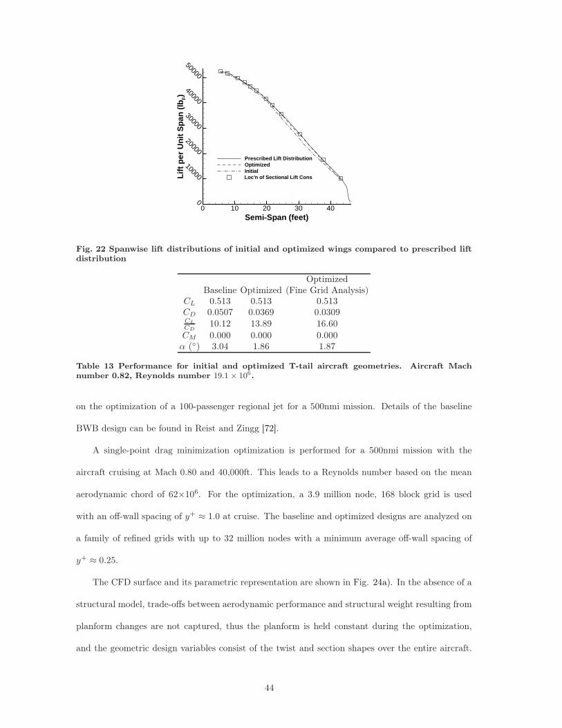
Semi-Span (feet)
Lift
per
Uni
t Spa
n (lb
F)
0 10 20 30 400
10000
20000
30000
40000
50000
Prescribed Lift DistributionOptimizedInitialLoc’n of Sectional Lift Cons
Fig. 22 Spanwise lift distributions of initial and optimized wings compared to prescribed liftdistribution
OptimizedBaseline Optimized (Fine Grid Analysis)
CL 0.513 0.513 0.513CD 0.0507 0.0369 0.0309CL
CD10.12 13.89 16.60
CM 0.000 0.000 0.000α (◦) 3.04 1.86 1.87
Table 13 Performance for initial and optimized T-tail aircraft geometries. Aircraft Machnumber 0.82, Reynolds number 19.1 × 10
6.
on the optimization of a 100-passenger regional jet for a 500nmi mission. Details of the baseline
BWB design can be found in Reist and Zingg [72].
A single-point drag minimization optimization is performed for a 500nmi mission with the
aircraft cruising at Mach 0.80 and 40,000ft. This leads to a Reynolds number based on the mean
aerodynamic chord of 62×106. For the optimization, a 3.9 million node, 168 block grid is used
with an off-wall spacing of y+ ≈ 1.0 at cruise. The baseline and optimized designs are analyzed on
a family of refined grids with up to 32 million nodes with a minimum average off-wall spacing of
y+ ≈ 0.25.
The CFD surface and its parametric representation are shown in Fig. 24a). In the absence of a
structural model, trade-offs between aerodynamic performance and structural weight resulting from
planform changes are not captured, thus the planform is held constant during the optimization,
and the geometric design variables consist of the twist and section shapes over the entire aircraft.
44

X/c
Cp
Z/c
0 0.2 0.4 0.6 0.8 1
-1
-0.5
0
0.5
1
1.5 -0.1
0
0.1
0.2
0.3
0.4
0.5
OptimizedBaseline
a) 10% Span
X/c
Cp
Z/c
0 0.2 0.4 0.6 0.8 1
-1
-0.5
0
0.5
1
1.5 -0.1
0
0.1
0.2
0.3
0.4
0.5
OptimizedBaseline
b) 26% Span
X/c
Cp
Z/c
0 0.2 0.4 0.6 0.8 1
-1
-0.5
0
0.5
1
1.5 -0.1
0
0.1
0.2
0.3
0.4
0.5
OptimizedBaseline
c) 42% Span
X/c
Cp
Z/c
0 0.2 0.4 0.6 0.8 1
-1
-0.5
0
0.5
1
1.5 -0.1
0
0.1
0.2
0.3
0.4
0.5
OptimizedBaseline
d) 58% Span
X/c
Cp
Z/c
0 0.2 0.4 0.6 0.8 1
-1
-0.5
0
0.5
1
1.5 -0.1
0
0.1
0.2
0.3
0.4
0.5
OptimizedBaseline
e) 74% Span
X/c
Cp
Z/c
0 0.2 0.4 0.6 0.8 1
-1
-0.5
0
0.5
1
1.5 -0.1
0
0.1
0.2
0.3
0.4
0.5
OptimizedBaseline
f) 90% Span
Fig. 23 T-tail aircraft wing sections and pressure distributions for initial and optimized ge-ometries
In addition, the angle-of-attack of the aircraft is a design variable and is constrained to be within
±3.0◦ such that the deck angle at cruise does not inhibit cabin operations. In order to maintain the
required space for a passenger compartment, a polyhedron representing the passenger compartment,
shown in Fig. 24b), forms a constraint such that the outer mold line cannot encroach upon the cabin.
In addition, the wing volume is constrained such that the required 4500gal fuel volume can fit within
80% of the wing outer mold line volume. The t/c of the sections over the entire aircraft are prevented
from decreasing by more than 25% of their initial value. In total there are 495 design variables.
Finally, the aircraft must be trimmed, that is at cruise CL = Wq∞S
= 0.23 and CM = 0 about the
center of gravity.
An Euler-based optimization is first performed in order to eliminate shocks in the inviscid design
space and obtain a more suitable starting point for the RANS-based optimization. While the Euler
optimized design is shock free, when analyzed with RANS the shocks return, but are weaker than
on the unoptimized baseline. From here on, “the baseline” shall refer to the Euler-optimized design
from which the RANS-based optimization is started. The optimization convergence history for the
45

a) Baseline BWB surface grids. B-splinecontrol points are shown as blue spheres
b) Polyhedron forming the cabin shapeconstraint
Fig. 24 The baseline BWB design
RANS-based optimization is shown in Fig. 25. At the end of the optimization the reduction in
the objective between iterations is insignificant, all constraints are satisfied, and the optimality has
been reduced by one order of magnitude. A 13.8% drag reduction is achieved over the baseline
design, as shown in Table 14. Most of this drag reduction comes from the elimination of the shock
as well as the reduction of separated flow, both of which are evident from the sectional pressure
distributions shown in Fig. 26. The shock on the baseline is evident from 50% of the span outboard,
as is its absence on the optimized design. While the initial Euler-based optimization achieved an
elliptic lift-distribution on the wing in the Euler design space, this is lost in the RANS space, as
seen in Fig. 27, due to the change in sectional loading caused by the reemergence of shocks and the
introduction of separation in the RANS solution. The lift distribution resulting from the RANS-
based optimization becomes more elliptical on the wing, but does not become perfectly elliptical.
The imposition of the cabin shape and trim constraint affect the load-carrying capacity of the
centerbody, which causes a deviation from the elliptical distribution. In addition, one would not
expect a perfectly elliptical spanload, which is a result of linear aerodynamics, in the RANS-based
optimization of a full-configuration for which the lifting surface is responsible for trim and whose
planform has significant sweep and chord changes, essentially leading to a nonplanar wake.
A grid convergence study is performed on both the baseline and optimized designs with a three-
member grid family of 8, 16, and 32 million node grids. The angle-of-attack is varied for each
grid to achieve the target lift. The pitching moment target is satisfied during the optimization,
but is not satisfied when the design is analyzed on the fine mesh. The results on both the finest
46
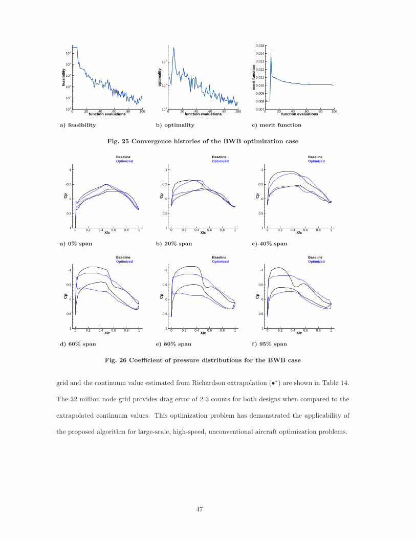
function evaluations
feas
ibili
ty
0 20 40 60 80 10010-8
10-7
10-6
10-5
10-4
10-3
a) feasibility
function evaluations
opti
mal
ity
0 20 40 60 80 10010-5
10-4
10-3
b) optimality
function evaluations
mer
it f
unct
ion
0 20 40 60 80 1000.007
0.008
0.009
0.010
0.011
0.012
0.013
0.014
0.015
c) merit function
Fig. 25 Convergence histories of the BWB optimization case
X/c
Cp
0 0.2 0.4 0.6 0.8 1
-1
-0.5
0
0.5
1
BaselineOptimized
a) 0% span
X/c
Cp
0 0.2 0.4 0.6 0.8 1
-1
-0.5
0
0.5
1
BaselineOptimized
b) 20% span
X/c
Cp
0 0.2 0.4 0.6 0.8 1
-1
-0.5
0
0.5
1
BaselineOptimized
c) 40% span
X/c
Cp
0 0.2 0.4 0.6 0.8 1
-1
-0.5
0
0.5
1
BaselineOptimized
d) 60% span
X/c
Cp
0 0.2 0.4 0.6 0.8 1
-1
-0.5
0
0.5
1
BaselineOptimized
e) 80% span
X/c
Cp
0 0.2 0.4 0.6 0.8 1
-1
-0.5
0
0.5
1
BaselineOptimized
f) 95% span
Fig. 26 Coefficient of pressure distributions for the BWB case
grid and the continuum value estimated from Richardson extrapolation (•∗) are shown in Table 14.
The 32 million node grid provides drag error of 2-3 counts for both designs when compared to the
extrapolated continuum values. This optimization problem has demonstrated the applicability of
the proposed algorithm for large-scale, high-speed, unconventional aircraft optimization problems.
47

2Y/b
Lift
0 0.2 0.4 0.6 0.8 10
0.05
0.1
0.15
0.2
Elli ptical distributionBaselineOptimized
Fig. 27 Lift distributions of the baseline and optimized BWB
Baseline OptimizedCL 0.230 0.230CD 0.0135 0.0118C∗
D 0.0132 0.0116CL
C∗
D
17.4 19.8
CM 0.0234 -0.0090α (◦) 4.65 2.40
Table 14 Performance of the baseline and optimized BWB designs. Continuum values areindicated with an asterisk, while remaining values are presented for the finest grid level.
VI. Conclusions
A methodology is presented for performing high-fidelity aerodynamic shape optimization in
steady turbulent flows. The integrated geometry parameterization and mesh movement methodology
is based on B-spline tensor volumes and produces a subset of B-spline control points on the surface
of the geometry that are used as design variables. High-fidelity numerical analysis based on the
three-dimensional RANS equations is performed using a parallel Newton-Krylov-Schur flow solver.
Constrained gradient-based optimization is carried out using SNOPT. The discrete-adjoint gradient
evaluation was developed by hand and treats the turbulence model in a fully coupled manner. The
evaluation includes a full hand linearization of the shock sensor.
Examples are presented to demonstrate the performance of the methodology for various aerody-
namic configurations in turbulent flow conditions, including conventional wing geometries, a wing-
body-tail configuration, and a blended wing-body configuration. The results show that geometries
produced in optimizations based on inviscid flow analysis are inferior to designs obtained based on
48

viscous analysis. A spanwise lift distribution constraint is imposed for the wing-body-tail configu-
ration. With this approach, the aerodynamic shape optimization reduces wave drag while having a
minimal effect on wing structure and hence its weight. The methodology is also shown to be capable
of robustly accommodating large changes in the geometry. Therefore the algorithm presented can
be used in the context of detailed design, exploratory aerodynamic shape optimization, or as the
aerodynamic module in a multidisciplinary optimization framework.
Acknowledgments
The authors gratefully acknowledge financial assistance from the Natural Sciences and Engineer-
ing Research Council (NSERC), the Ontario Graduate Scholarship program, the Canada Research
Chairs program, Bombardier Aerospace, and the University of Toronto.
Computations were performed on the GPC supercomputer at the SciNet HPC Consortium, part
of Compute Canada.
References
[1] “Boeing 787 Dreamliner provides new solutions for airlines, passengers,” Tech. rep., Boeing, Seattle,
WA, USA, 2013.
[2] “A350 XWB: Shaping efficiency,” Tech. rep., Airbus, Toulouse, France, 2013.
[3] “X-48 Research: All good things must come to an end,” Tech. rep., NASA, Edwards, CA, USA, 2013.
[4] Reist, T. A. and Zingg, D. W., “Aerodynamic shape optimization of a Blended-Wing-Body regional
transport for a short range mission,” 31st AIAA Applied Aerodynamics Conference, AIAA–2013–2414,
San Diego, CA, USA, June 2013.
[5] Drela, M., “Simultaneous optimization of the airframe, powerplant, and operation of transport aircraft,”
In RAeS 2nd Aircraft Structural Design Conference, Hamilton Place, London, 2010.
[6] Rogers, M. M., “Technical challenges to reducing subsonic transport drag,” 50th AIAA Aerospace Sci-
ences Meeting , Nashville, TN, USA, Jan. 2012, http://ntrs.nasa.gov/search.jsp?R=20120006660.
[7] Gallman, J. W. and Kroo, I. M., “Structural optimization for joined-wing synthesis,” Journal of Aircraft,
Vol. 33, No. 1, 1996, pp. 214–223.
[8] Hicks, R. M. and Henne, P. A., “Wing design by numerical optimization,” Journal of Aircraft, Vol. 15,
No. 7, July 1978, pp. 407–412.
49

[9] Pironneau, O., “On optimum design in fluid mechanics,” Journal of Fluid Mechanics, Vol. 64, No. 1,
1974, pp. 97–110.
[10] Jameson, A., “Aerodynamic design via control theory,” Journal of Scientific Computing , Vol. 3, No. 3,
1988, pp. 233–260.
[11] Anderson, W. K. and Bonhaus, D. L., “Airfoil design on unstructured grids for turbulent flows,” AIAA
Journal , Vol. 37, No. 2, Feb. 1999, pp. 185–191.
[12] Nemec, M. and Zingg, D. W., “Newton-Krylov algorithm for aerodynamic design using the Navier-
Stokes equations,” AIAA Journal , Vol. 40, No. 6, 2002, pp. 1146–1154.
[13] Nemec, M., Zingg, D. W., and Pulliam, T. H., “Multipoint and multi-objective aerodynamic shape
optimization,” AIAA Journal , Vol. 42, No. 6, 2004, pp. 1057–1065.
[14] Buckley, H. P. and Zingg, D. W., “An approach to aerodynamic design through numerical optimization,”
AIAA Journal , Vol. 51, No. 8, 2013, pp. 1972–1981.
[15] Driver, J. and Zingg, D. W., “Numerical aerodynamic optimization incorporating laminar-turbulent
transition prediction,” AIAA Journal , Vol. 45, No. 8, Aug. 2007, pp. 1810–1818.
[16] Hicken, J. and Zingg, D., “Induced drag minimization of nonplanar geometries based on the Euler
equations,” AIAA Journal , Vol. 48, No. 11, 2010, pp. 2564–2575.
[17] Elliott, J. and Peraire, J., “Aerodynamic optimization on unstructured meshes with viscous effects,”
13th AIAA Computational Fluid Dynamics Conference, AIAA–97–1849, Snowmass, Colorado, June
1997.
[18] Elliott, J. K., Aerodynamic optimization based on the Euler and Navier-Stokes equations using un-
structured grids, Ph.D. thesis, Massachusetts Institute of Technology, Cambridge, Massachusetts, USA,
1998.
[19] Jameson, A., Martinelli, L., and Pierce, N. A., “Optimum aerodynamic design using the Navier-Stokes
equations,” Theoretical and Computational Fluid Dynamics, Vol. 10, 1998, pp. 213–237.
[20] Nielsen, E. J. and Anderson, W. K., “Aerodynamic design optimization on unstructured meshes using
the Navier-Stokes equations,” AIAA Journal , Vol. 37, No. 11, Nov. 1999, pp. 1411–1419.
[21] Brezillon, J., Brodersen, O., Dwight, R., Ronzheimer, A., and Wild, J., “Development and application
of a flexible and efficient environment for aerodynamic shape optimisation,” Proceedings of the ONERA-
DLR Aerospace Symposium (ODAS), Toulouse, 2006.
[22] Brezillon, J. and Dwight, R. P., “Applications of a discrete viscous adjoint method for aerodynamic
shape optimisation of 3D configurations,” CEAS Aeronautical Journal , Vol. 3, No. 1, 2012, pp. 25–34.
[23] Epstein, B., Jameson, A., Peigin, S., Roman, D., Harrison, N., and Vassberg, J., “Comparative study
50

of 3D wing drag minimization by different optimization techniques,” 46th AIAA Aerospace Sciences
Meeting and Exhibit, AIAA–2008–326, Reno, Nevada, Jan. 2008.
[24] Sobieszczanski-Sobieski, J. and Haftka, R. T., “Multidisciplinary aerospace design optimization: survey
of recent developments,” Structural optimization, Vol. 14, No. 1, 1997, pp. 1–23.
[25] Alexandrov, N. M. and Hussaini, M. Y., Multidisciplinary design optimization: State of the art, Vol. 80,
SIAM, 1997.
[26] Leoviriyakit, K., Kim, S., and Jameson, A., “Aero-structural wing planform optimization using the
Navier-Stokes equations,” 10th AIAA/ISSMO Multidisciplinary Analysis and Optimization Conference,
AIAA–2004–4479, Albany, New York, Aug. 2004.
[27] Martins, J. R. R. A., Alonso, J. J., and Reuther, J. J., “High-fidelity aerostructural design optimization
of a supersonic business jet,” Journal of Aircraft, Vol. 41, No. 3, May 2004, pp. 863–873.
[28] Kenway, G. K. W. and Martins, J. R. R. A., “Multi-point high-fidelity aerostructural optimization of a
transport aircraft configuration,” Journal of Aircraft, 2014, (In press).
[29] Kenway, G. K. W., Kennedy, G. J., and Martins, J. R. R. A., “A scalable parallel approach for high-
fidelity steady-state aeroelastic analysis and derivative computations,” AIAA Journal , 2014, (In press).
[30] Barcelos, M. and Maute, K., “Aeroelastic design optimization for laminar and turbulent flows,” Com-
puter Methods in Applied Mechanics and Engineering, Vol. 197, No. 19–20, 2013, pp. 1813–1832.
[31] Ghazlane, I., Carrier, G., Dumont, A., and Désidéri, J., “Aerostructural adjoint method for flexible wing
optimization,” 53rd AIAA/ASME/ASCE/AHS/ASC Structures, Structural Dynamics, and Materials
Conference, AIAA–2012–1924, Honolulu, HI, April 2012.
[32] Brezillon, J., Ronzheimer, A., Haar, D., Abu-Zurayk, M., Lummer, K., Krugër, W., and Nattere,
F. J., “Development and application of multi-disciplinary optimization capabilities based on high-fidelity
methods,” 53rd AIAA/ASME/ASCE/AHS/ASC Structures, Structural Dynamics, and Materials Con-
ference, AIAA–2012–1757, Honolulu, HI, April 2012.
[33] Kulfan, B. M., “A universal parametric geometry representation method — “CST”,” The 45th AIAA
Aerospace Sciences Meeting and Exhibit, AIAA–2007–0062, Reno, Nevada, 2007.
[34] Mohammadi, B., “A new optimal shape design procedure for inviscid and viscous turbulent flows,”
International Journal for Numerical Methods in Fluids, Vol. 25, No. 2, July 1997, pp. 183–203.
[35] Nemec, M. and Aftosmis, M. J., “Aerodynamic shape optimization using a Cartesian adjoint method
and CAD geometry,” 24th AIAA Applied Aerodynamics Conference, AIAA–2006–3456, San Francisco,
California, United States, June 2006.
[36] Sederberg, T. W. and Parry, S. R., “Free-form deformation of solid geometric models,” SIGGRAPH
51

’86: Proceedings of the 13th annual conference on Computer graphics and interactive techniques, ACM,
New York, NY, USA, 1986, pp. 151–160.
[37] Gagnon, H. and Zingg, D. W., “Geometry generation of complex unconventional aircraft with appli-
cation to high-fidelity aerodynamic shape optimization,” 21st AIAA Computational Fluid Dynamics
Conference, AIAA–2013–2850, San Diego, CA, United Sates, June 2013.
[38] Anderson, W. K., Karman, S. L., and Burdyshaw, C., “Geometry parameterization method for multi-
disciplinary applications,” AIAA Journal , Vol. 47, No. 6, 2009, pp. 1568–1578.
[39] Burgreen, G. W. and Baysal, O., “Three-dimensional aerodynamic shape optimization using discrete
sensitivity analysis,” AIAA Journal , Vol. 34, No. 9, Sept. 1996, pp. 1761–1770.
[40] Osusky, L. and Zingg, D. W., “Application of an efficient Newton-Krylov algorithm for aerodynamic
shape optimization based on the Reynolds-averaged Navier-Stokes equations,” 21st AIAA Computa-
tional Fluid Dynamics Conference, AIAA–2013–2584, San Diego, CA, United States, June 2013.
[41] Lépine, J., Guilbault, F., Trépanier, J.-Y., and Pépin, F., “Optimized nonuniform rational B-spline
geometrical representation for aerodynamic design of wings,” AIAA Journal , Vol. 39, No. 11, Nov.
2001, pp. 2033–2041.
[42] Hicken, J. E. and Zingg, D. W., “Aerodynamic optimization algorithm with integrated geometry pa-
rameterization and mesh movement,” AIAA Journal , Vol. 48, No. 2, Feb. 2010, pp. 400–413.
[43] Rogers, D. F. and Adams, J. A., Mathematical Elements for Computer Graphics, McGraw–Hill, Inc.,
New York, NY, 1990.
[44] Truong, A. H., Oldfield, C. A., and Zingg, D. W., “Mesh movement for a discrete-adjoint Newton-Krylov
algorithm for aerodynamic optimization,” AIAA Journal , Vol. 46, No. 7, July 2008, pp. 1695–1704.
[45] Meijerink, J. A. and van der Vorst, H. A., “An iterative solution method for linear systems of which
the coefficient matrix is a symmetric M-matrix,” Mathematics of Computation, Vol. 31, No. 137, Jan.
1977, pp. 148–162.
[46] Hicken, J. E. and Zingg, D. W., “A parallel Newton-Krylov solver for the Euler equations discretized
using simultaneous approximation terms,” AIAA Journal , Vol. 46, No. 11, Nov. 2008, pp. 2773–2786.
[47] Osusky, M. and Zingg, D. W., “Parallel Newton-Krylov-Schur flow solver for the Navier-Stokes equations
discretized using summation-by-parts operators,” AIAA Journal , Vol. 51, No. 12, 2013, pp. 2833–2851.
[48] Pulliam, T. H. and Zingg, D. W., Fundamental Algorithms in Computational Fluid Dynamics, Springer,
2014.
[49] Carpenter, M. H., Gottlieb, D., and Abarbanel, S., “Time-stable boundary conditions for finite-
difference schemes solving hyperbolic systems: methodology and application to high-order compact
52

schemes,” Journal of Computational Physics, Vol. 111, No. 2, 1994, pp. 220–236.
[50] Hesthaven, J. S., “A stable penalty method for the compressible Navier-Stokes equations: III. Multi-
dimensional domain decomposition schemes,” SIAM Journal on Scientific Computing , Vol. 20, No. 1,
1998, pp. 62–93.
[51] Carpenter, M. H., Nordström, J., and Gottlieb, D., “A stable and conservative interface treatment of
arbitrary spatial accuracy,” Journal of Computational Physics, Vol. 148, No. 2, 1999, pp. 341–365.
[52] Nordström, J. and Carpenter, M. H., “High-order finite difference methods, multidimensional linear
problems, and curvilinear coordinates,” Journal of Computational Physics, Vol. 173, No. 1, 2001,
pp. 149–174.
[53] Osusky, M. and Zingg, D. W., “A parallel Newton-Krylov-Schur flow solver for the Navier-Stokes
equations using the SBP-SAT approach,” 50th AIAA Aerospace Sciences Meeting , AIAA–2012–0442,
Nashville, TN, United States, Jan. 2012.
[54] Svärd, M., Carpenter, M. H., and Nordström, J., “A stable high-order finite difference scheme for
the compressible Navier-Stokes equations, far-field boundary conditions,” Journal of Computational
Physics, Vol. 225, No. 1, July 2007, pp. 1020–1038.
[55] Svärd, M. and Nordström, J., “A stable high-order finite difference scheme for the compressible Navier-
Stokes equations, no-slip wall boundary conditions,” Journal of Computational Physics, Vol. 227, No. 10,
May 2008, pp. 4805–4824.
[56] Nordström, J., Gong, J., van der Weide, E., and Svärd, M., “A stable and conservative high order
multi-block method for the compressible Navier-Stokes equations,” Journal of Computational Physics,
Vol. 228, No. 24, 2009, pp. 9020–9035.
[57] Kreiss, H. O. and Scherer, G., “Finite element and finite difference methods for hyperbolic partial dif-
ferential equations,” Mathematical Aspects of Finite Elements in Partial Differential Equations, edited
by C. de Boor, Mathematics Research Center, the University of Wisconsin, Academic Press, 1974.
[58] Strand, B., “Summation by parts for finite difference approximations for d/dx,” Journal of Computa-
tional Physics, Vol. 110, No. 1, 1994, pp. 47–67.
[59] Saad, Y. and Sosonkina, M., “Distributed Schur complement techniques for general sparse linear sys-
tems,” SIAM Journal of Scientific Computing , Vol. 21, No. 4, 1999, pp. 1337–1357.
[60] Hicken, J. E., Efficient algorithms for future aircraft design: Contributions to aerodynamic shape opti-
mization, Ph.D. thesis, University of Toronto, Toronto, Ontario, Canada, 2009.
[61] Osusky, L., A numerical methodology for aerodynamic shape optimization in turbulent flow enabling
large geometric variation, Ph.D. thesis, University of Toronto, Toronto, Ontario, Canada, 2014.
53
[62] de Sturler, E., “Nested Krylov methods based on GCR,” Journal of Computational and Applied Math-
ematics, Vol. 67, 1996, pp. 15–41.
[63] de Sturler, E., “Truncation strategies for optimal Krylov subspace methods,” SIAM Journal on Numer-
ical Analysis, Vol. 36, No. 3, 1999, pp. 864–889.
[64] Hicken, J. E. and Zingg, D. W., “A simplified and flexible variant of GCROT for solving nonsymmetric
linear systems,” SIAM Journal on Scientific Computing , Vol. 32, No. 3, June 2010, pp. 1672–1694.
[65] Gill, P. E., Murray, W., and Saunders, M. A., “SNOPT: an SQP algorithm for large-scale constrained
optimization,” SIAM Journal on Optimization, Vol. 12, No. 4, 2002, pp. 979–1006.
[66] Zingg, D. W., Nemec, M., and Pulliam, T. H., “A comparative evaluation of genetic and gradient-
based algorithms applied to aerodynamic optimization,” European Journal of Computational Mechanics,
Vol. 17, 2008, pp. 103–126.
[67] Chernukhin, O. and Zingg, D. W., “Multimodality and global optimization algorithms for aerodynamic
shape optimization,” AIAA Journal , Vol. 51, No. 6, 2013, pp. 1342–1354.
[68] Zingg, D., Leung, T., Diosady, L., Truong, A., Elias, S., and Nemec, M., “Improvements to a Newton-
Krylov algorithm for aerodynamic shape optimization,” 43rd AIAA Aerospace Sciences Meeting and
Exhibit , AIAA–2005–4857, Reno, Nevada, 2005.
[69] Vassberg, J. C., Tinoco, E. N., Mani, M., Rider, B., Zickuhr, T., Levy, D. W., Brodersen, O. P.,
Eisfeld, B., Crippa, S., Wahls, R. A., Morrison, J. H., Mavriplis, D. J., and Murayama, M., “Summary
of the Fourth AIAA CFD Drag Prediction Workshop,” 28th AIAA Applied Aerodynamics Conference,
AIAA–2010–4547, Chicago, Illinois, United States, June 2010.
[70] Levy, D. W., Laflin, K. R., Tinoco, E. N., Vassberg, J. C., Mani, M., Rider, B., Rumsey, C. L., Wahls,
R. A., Morrison, J. H., Brodersen, O. P., Crippa, S., Mavriplis, D. J., and Murayama, M., “Summary of
data from the Fifth AIAA CFD Drag Prediction Workshop,” 51st AIAA Aerospace Sciences Meeting
and Aerospace Exposition, AIAA–2013–0046, Grapevine, Texas, United States, Jan. 2013.
[71] “ANSYS ICEM CFD Tutorial Manual,” Tech. Rep. ANSYS ICEM CFD 14.0, ANSYS, Inc., 2011,
http://www.ansys.com.
[72] Reist, T. A. and Zingg, D. W., “Aerodynamically Optimal Regional Aircraft Concepts: Conventional
and Blended Wing-Body Designs,” 52nd AIAA Aerospace Sciences Meeting , AIAA-2014-0905, National
Harbor, MD, January 2014.
54