Embed Size (px)
Citation preview
MCAT Institute
Final Report94-004
NASA-CR-195094/ J,
/
DEVELOPMENT OF ADVANCEDNAVIER-STOKES SOLVER
Seokkwan Yoon
(NASA-CR-195094) DEVELOPMENT
ADVANCED NAVIeR-STOKES SOLVER
(MCAT Inst.) 20 p
OF N94-37449
unclas
G3/64 0016036
June 1994 NCC2-505
MCAT Institute3933 Blue Gum Drive
San Jose, CA 95127
https://ntrs.nasa.gov/search.jsp?R=19940032941 2019-02-21T20:30:17+00:00Z

I. Introduction
Scope
The objective of research was to develop and validate new computational algorithms for
solving the steady and unsteady Euler and Navier-Stokes equations. The end-products are
new three-dimensional Euler and Navier-Stokes codes that are faster, more reliable, more
accurate, and easier to use.
Approach
The three-dimensional Euler and full/thin-layer Reynolds-averaged Navier-Stokes equa-
tions for compressible/incompressible flows are solved on structured hexahedral grids. The
Baldwin-Lomax algebraic turbulence model is used for closure. The space discretization is
based on a cell-centered finite-volume method augmented by a variety of numerical dissi-
pation models with optional total variation diminishing limiters. The governing equations
are integrated in time by an implicit method based on lower-upper factorization and sym-
metric Gauss-Seidel relaxation. The algorithm is vectorized on diagonal planes of sweep
using two-dimensional indices in three dimensions. Convergence rates and the robustness
of the codes are enhanced by the use of an implicit full approximation storage multigridmethod.
II. Previous Results
Previous results obtained under this cooperative agreement were reported in MCAT Progress
Reports submitted in Feb. '93, Oct. '92, Apr. '92, and Oct. '89.
III. Current Work
A new computer program named CENS3D-MG has been developed for compressible flows
with discontinuities. Details of the code are described in Appendix A and Appendix B.
IV. Summary and Conclusions
The improved computational efficiency of the Navier-Stokes solvers by the use of a highly
vectorizable and unconditionally stable algorithm makes fine grid calculations affordable.
The resulting code is fast enough to be used as an aerodynamic design tool for advanced
subsonic and supersonic transport aircrafts.

APPENDIX- A

Multigrid Convergence of an ImplicitSymmetric Relaxation Scheme
Seokkwan YoonandDochan KwakMCAT InstituteMoffett FieldCalifornia

AIAA JOURNAL
Vol. 32, No. 5, May 1994
Multigrid Convergence of an Implicit SymmetricRelaxation Scheme
Seokkwan Yoon* and Dochan Kwak?
NASA Ames Research Center, Moffett Field, California 94035
The multigrid method has been applied to an existing three-dimensional compressible Euler solver toaccelerate the convergence of the implicit symmetric relaxation scheme. This lower-upper symmetric Gauss-Seidel implicit scheme is shown to be an effective multigrid driver in three dimensions. A grid refinement studyis performed including the effects of large cell aspect ratio meshes. Performance figures of the present multigrid
code on Cray computers including the new C90 are presented. A reduction of three orders of magnitude in theresidual for a three-dimensional transonic inviscid flow using 920 k grid points is obtained in less than 4 min ona Cray C90.
I. Introduction
LTHOUGH unstructured grid methods have been usedsuccessfully in solving the Euler equations for complex
geometries, structured grid solvers still remain useful for the
Navier-Stokes equations because of their natural advantages
in dealing with the highly clustered meshes in the viscous
boundary layers. Structured grid methods not only handle
reasonably complex geometries using multiple blocks but also
offer a hybrid grid scheme to alleviate difficulties which un-structured grid methods have often encountered. Recent de-
velopments in structured grid solvers have been focused on
efficiency, as well as accuracy, since most existing three-di-
mensional Navier-Stokes codes are still not efficient enough to
be used routinely for aerodynamic design.
Multigrid methods have been useful for accelerating the
convergence of iterative schemes. Efficient Euler codes havebeen developed by Jameson t using a full approximation stor-
age method of Brandt z in conjunction with the explicit Runge-
Kutta scheme. The explicit multigrid method has demon-
strated impressive convergence rates by taking large time steps
and propagating waves fast on coarse meshes. The explicitmultigrid method has been extended to the Navier-Stokes
equations by Martinelli. 3 Several explicit multigrid codes for
the three-dimensional Navier-Stokes equations have been de-
veloped successfully by Vatsa and Wedan, 4 Radespiel et al., 5and Turkel et al.6
It does not seem to be pr(afit-able to consider an unfactored
implicit scheme for a multigrid driver since the implicit scheme
can take large time steps which are limited by the physics rather
than the grid. However, the multigrid method can improve the
convergence rates of factored implicit schemes in two dimen-sions as demonstrated by Yoon 7 and in Refs. 8-10. The im-
plicit multigrid method has been implemented by Caughey ]2 to
the diagonalized alternating direction scheme, i t and by Ander-son et alY to the three-dimensional alternating direction
scheme. Yoon 7 has introduced an implicit algorithm based on
a lower-upper (LU) factorization and symmetric Gauss-Seidel
(SGS) relaxation. The scheme has been used successfully in
Received May 17, 1993; presented as Paper 93-3357 at the AIAAComputational Fluid Dynamics Conference, Orlando, FL, July 6--9,1993; revision received Oct. 4, 1993; accepted for publication Oct. 13,1993. Copyright © 1993 by the American Institute of Aeronautics andAstronautics, Inc. No copyright is asserted in the United States underTitle 17, U.S. Code. The U.S. Government has a royalty-free licenseto exercise all rights under the copyright claimed herein for Govern-mental purposes. All other rights are reserved by the copyright owner.
*Research Scientist, Computational Algorithms and ApplicationsBranch.
t-Chief, Computational Algorithms and Applications Branch.
computing chemically reacting flows due in part to the al-
gorithm's property which reduces the size of the left-hand sidematrix for nonequilibrium flows with finite rate chemis-
try. t4-t6 A recent study t7 shows that the three-dimensional
extension of the method using a single grid requires less com-
putational time than most existing codes on a Cray YMP
computer. One of the objectives of the present work is to
accelerate the convergence of the lower-upper symmetricGauss-Seidel relaxation scheme in three dimensions by intro-
ducing a multigrid technique. The performance of the code is
demonstrated for an inviscid transonic flow past an ONERA
M6 wing on highly clustered grids.
II. Governing Equations
Let t be time; _ the vector of conserved variables;/_, P', and(_ the convective flux vectors; and -_, Pv, and (_, the flux
vectors for the viscous terms. Then the three-dimensional
Navier-Stokes equations in generalized curvilinear coordinates
(/_, 71, _') can be written as
atL)+ a_(_"- $.)+ o.(P-t'.)+ ago - 0,) = o (1)
where the flux vectors are defined in Ref. 17. The Euler
equations are obtained by neglecting the viscous terms.
950
III. Lower-Upper Symmetric Gauss-SeidelImplicit Scheme
An unfactored implicit scheme can be obtained from a
nonlinear implicit scheme by linearizing the flux vectors about
the previous time step and dropping terms of the second and
higher order.
[I + ez%t(Di_t + D_]3 + D_')I6Q = -_t_ (2)
where the residual/_ is
(3)
and I is the identity matrix. The correction _Y' + 1 _ _, is _.,
where n denotes the time level. DI, D r, and D r are differenceoperators that approximate a t, a_, and a¢, respectively. ,,_,/),and _7 are the Jacobian matrices of the convective flux vectors.
For a = IA, the scheme is second-order accurate in time. For
other values of _, the time accuracy drops to first order.
An efficient implicit scheme can be derived by combining
the advantages of LU factorization and Gauss-Seidel relaxation.
LD - ' U6_ = - At2_ (4)
HMliK;IU, Ww4i PAGE BLANK NOT FILMED

Here,
L = I + c_At(D_-_* +D_-B ÷ +DF_ + -.?4- -B--O-)
D= l + ou_t(_l ÷ - 21- + [3* -[3- + _* -dr-) (5)
U = I +_z_t(D_+71- + D;[3- +D(O- +A * +[3+ + _*)
where D(, D,-, and D:- are backward difference operators,
while D(, D_+, and D_+ are forward difference operators.
In the framework of the LU-SGS algorithm, a variety ofschemes can be developed by different choices of numerical
dissipation models and Jacobian matrices of the flux vectors.
Jacobian matrices leading to diagonal dominance are con-
structed so that + matrices have non-negative eigenvalues
whereas - matrices have nonpositive eigenvalues. For example,
(6)
where typically T_ and 7"_- 1 are similarity transformation ma-
trices of the eigenvectors of ,4. Another possibility is to con-
struct the Jacobian matrices of the flux vectors approximatelywhich yield diagonal dominance.
,21* = ½[.21 + k(_l)ll
[3- = ,/2[[3+ k([3)II (7)
dr* = ½ [dr + _(d3II
Here, the conserved variables are averaged at the cell faces to
evaluate the fluxes. The dissipative flux d is added to theconvective flux in a conservative manner.
+ _i.j.k+ !,: -- _i.j.k-'.':)-- ( di÷ :.:.j.k -- di-:.j.l¢
+di.j+v_.k-di.j-v,.k +di, j.,.,/_-di.j.,__/:) (13)
For simplicity, d_÷ ,/,.j., is denoted by d_. ,/, hereafter.
-(_ ._(0.,., - 0.)di+ ,/: = ei+
.(4) ,/,(_.i + 2 30.i +, + 3Oi Oi- 1) (14)-- _l+ -- --
The coefficients of the dissipative terms are the directionallyscaled spectral radii of the Jacobian matrices. The use of
directional scaling provides anisotropic dissipation to eachdirection, resulting in improved performance on meshes with
high aspect ratio cells. Third-order terms formed from fourth
differences provide the background damping. First-orderterms are added by second differences near shock waves underthe control of a sensor _.
vi÷ '/: = max(;'i+ t, ui) (15)
where
"i = max(vf, _r) (16)
uPi = Ipi*l--2pi+Pi-II/(P_+t+2pi+pi-O (17)
vf= IT,+_-2T,+T_-tl/(Ti+t+2Ti+Ti_O (18)
where
_(_) = _ maxllX(,71)ll (8)
Here X(,4) represents eigenvalues of the Jacobian matrix .21,
and _ is a constant that is greater than or equal to 1. A typical
value of _ is 1. However, stability and convergence can be
controlled by adjusting x as the flowfield develops.
Here p and T are the pressure and the temperature. The
low-order dissipative coefficient is proportional to the sensoras
_I;_ ) vl = K_2)r(/l)i+ v_÷ '/_ (19)
where r(,21) denotes the spectral radius of the Jacobian matrix
,21. The high-order dissipative coefficient is controlled by thesensor.
IV. Vectorization
The algorithm is completely vectorizable on i+j +k =
const diagonal planes of sweep. This is achieved by reorderingthe arrays.
_(ipoint, /plane) = _.(i, j, k) (9)
where/plane is the serial number of the diagonal plane, and
/point is the address on that plane. The number of diagonalplanes is given by
nplane = imax +jmax + kmax - 5
with the maximum vector length of
(10)
npoint = (jmax- 1)*(kmax- 1) (11)
V. Numerical Dissipation
The cell-centered finite-volume method is augmented by a
numerical dissipation model based on blended first- and third-order terms. _a-2_ The finite volume method is based on the
local flux balance of each mesh cell. For example,
(12)
e(4) = max[0,x(4)r (_[)i + ,/_ _(2)i+ '/, - _i+ ,_] (20)
Here _¢2) and x,4_are constants which are different from other
in Eq. (8).
Dissipative terms for the coarse grids in the multigrid levelsare formed from second differences with constant coefficients.
Since the constant total enthalpy is not preserved in general
except for the Euler equations, the dissipation for the energyequation is based on the total energy rather than the total
enthalpy. To reduce the amount of dissipation in the direction
normal to the body surface inside boundary layers, Swanson
and Turkeff ° provided additional scaling by multiplying a
spectral radius in the normal direction by a function of the
local Mach number. Although the Math number scaling tech-nique may improve the accuracy of the Navier-Stokes solu-
tions, it has not been used for the Euler solutions. It has been
shown that the convergence rate on high cell aspect ratio
meshes can be enhanced by multiplying Martinelli's 3 scaling
factor based on local cell aspect ratio to the dissipative coeffi-cients. However, this technique has not been used here be-
cause the aspect ratio based scaling factor seems to compro-mise the accuracy of the solution, z2
VI. Multigrid Method
In the present multigrid method, part of the task of tracking
the evolution of the solution is transferred through a sequence
of successively coarser meshes. The use of larger control vol-
umes on the coarser meshes tracks the large-scale evolution,

withtheconsequencethatglobalequilibriumcanbemorerapidlyattained.This evolution on the coarse grid is driven by
the solution of the fine grid equations. The solution vector on
a coarse grid is initialized as
Q¢O_= _,ShQh / S_ (21)2h
where the subscripts denote values of the mesh spacing param-
eter h, S is the cell volume, and the sum is over the eight cells
of the fine grid which compose each cell of the coarse grid.After updating the fine grid solution, the values of the con-
served variables are transferred to the coarse grid using Eq.
(21). The pressure is calculated on the coarse grid using the
transferred variables. Then a forcing function is defined as
---(0))P:h = _.Rh(Q^) - R2,(_2_,. (22)
The residual on the coarse grid is given by
Rz_ = R2h(Q2h) + P_ (23)
For the next coarser grid, the residual is calculated as
R_ = R4h(Q4h) + Pah (24)
where
P4h = _R_ - R4h(Q_°h )) (25)
2
o 10 ]
4.J
10' ............................
<
10 60 80 100 120 140
Streamwise Grid Index i
Fig. l Distribution of cell aspect ratios (CAR) for the low CAR grid(140 k grid points).
l°°l i
t ii i i -.- I levilO , I.... I" ! _ -- 4 level V'2
-2. ,......_.................i.........................:,.........................;.........................
to t: ', i ! i
lO_ i..............?:_"".__ ..... i; i x i i
-4 .......':............i......................2:.:.,.........................i......................
l0 "i
10 0 500 lO00 1500 2000
Iterations
Fig. 2 Convergence histories on the low CAR grid.
O
r_
<
10
5
10
4
10
3
l0
10 100 150 200 250 300
Streamwise Grid Index i
Fig. 3 Distribution of cell aspect ratios for the high CAR grid (920 kgrid points).
-| .....................................................................................................
lO i i
-5
10 0 500 1000 1500 2000
Iterations
Fig. 4 Convergence histories for the Euler and Navier-Stokes equa-tions.
The process is repeated on successively coarser grids. Multiple
iterations can be done on each coarse grid. Finally, the correc-
tion calculated on each grid is interpolated back to the next
finer grid. Let _.2, be the final value of Q_ resulting from both
the correction calculated on grid 2h and the correction trans-
ferred from the grid 4h. Then
_ = Qh + l_(_2h - Q_) (26)
where Q_ is the solution on grid h before the transfer to the
grid 2h, and I is a trilinear interpolation operator. Since theevolution on a coarse grid is driven by residuals collected from
the next finer grid, the final solution on the fine grid is
independent of the choice of boundary conditions on the
coarse grids.
VII. Results
To investigate the effectiveness of the full approximation
storage multigrid method in conjunction with the lower-upper
symmetric Ganss-Seidel relaxation scheme, transonic flow cal-culations have been carried out for an ONERA M6 wing. The
frees(ream conditions are at a Mach number of 0.8395, and a
3.06-deg angle of attack. Since this is an unseparated flow
case, only the solution of the three-dimensional Euler equa-tions is considered.
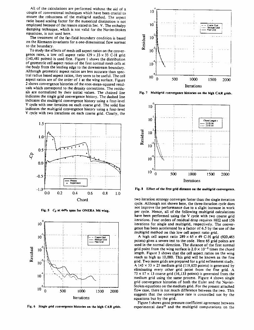
All ofthecalculationsareperformedwithouttheaidof acoupleofconventionaltechniqueswhichhavebeencrucialtoensuretherobustnessof themultigridmethod.The aspectratio based scaling factor for the numerical dissipation is not
employed because of the reason stated in Sec. V. The enthalpydamping technique, which is not valid for the Navier-Stokesequations, is not used here.
The treatment of the far-field boundary condition is based
on the Riemann invariants for a one-dimensional flow normal
to the boundary.
To study the effects of mesh cell aspect ratios on the conver-
gence rates, a low cell aspect ratio 129 x 33 x 33 C-H grid
(140,481 points) is used first. Figure 1 shows the distributionof geometric cell aspect ratios of the first normal mesh cells at
the body from the leading edge to the downstream boundary.
Although geometric aspect ratios are less accurate than spec-
tral radius based aspect ratios, they seem to be useful. The cell
aspect ratios are of the order of 1 at the wing surface. Figure
2 shows convergence histories of the root-mean-squared resid-
uals which correspond to the density corrections. The residu-
als are normalized by their initial values. The chained line
indicates the single grid convergence history. The dashed line
indicates the multigrid convergence history using a four-level
V cycle with one iteration on each coarse grid. The solid line
indicates the muitigrid convergence history using a four-level
V cycle with two iterations on each coarse grid. Clearly, the
1511.0-
0.5-
0.0-
-0.5
-1.00.0 0'.2
-- Prl_nt [• Exl_tirnent
014 0'.6 0.8 1.0
Chord
Fig. 5 Cp at 44% span for ONERA M6 wing.
i0°i
-4
10
-5
10
,"................................................ [ ....... -.- Coarse Grkl ...........
l _ _ .... Meditan Grid I I
.................i....................!....................!......................
2
0 500 1000 1500 2000
Iterations
Fig. 6 Single grid convergence histories on the high CAR grids.
_J
Fig. 7
10
-I.
10
lO_
103!
-4
10
-5
10
J-. - Ctwase Grid.... M¢_mri Grid-- Free Grid
0 500 1000 1500 2000
Iterations
Multigrid convergence histories on the high CAR grids.
10_
-| .....................................................
10 c_-_ t_, I2.0 E-06
.... 2.0 E-05
10 2 .......................................................................................................
lO.;la .............i..................................................i........................10 0 500 1000 1500 2000
Iterations
Fig. 8 Effect of the first grid distance on the multigrld convergence.
two iteration strategy converges faster than the single iteration
cycle. Although not shown here, the three-iteration cycle doesnot improve the performance due to a slight increase in work
per cycle. Hence, all of the following multigrid calculations
have been performed using the V cycle with two coarse griditerations. Four orders of residual drop requires 1022 and 156
iterations for single and multigrid, respectively. The conver-
gence has been accelerated by a factor of 6.5 by the use of the
multigrid method on this low cell aspect ratio grid.
A high cell aspect ratio 289 x 65 x 49 C-H grid (920,465
points) gives a severe test to the code. Here 65 grid points areused in the normal direction. The distance of the first normal
grid point from the wing surface is 2.0 x 10 -6 times the chord
length. Figure 3 shows that the cell aspect ratios on the wing
reach as high as 10,000. This grid will be known as the finegrid. Two more grids are prepared for a grid refinement study.
A 145 × 33 × 25 medium grid (119,625 points) is generated byeliminating every other grid point from the fine grid. A
73 × 17 x 13 coarse grid (16,133 points) is generated from the
medium grid using the same process. Figure 4 shows single
grid convergence histories of both the Euler and the Navier-
Stokes equations on the medium grid. For the present attachedflow case, there is not much difference between the two. This
suggests that the convergence rate is controlled not by the
equations but by the grid.
Figure 5 shows good pressure coefficient agreement betweenexperimental data 23 and the multigrid computations on the

Y()()N ;_NI) K'_r,_K - IMPLICtFSv',.t',,tFg_C_,EL.:,,.:._TO_'SCuE_,_rE ..................
Fig. 9
10
10.1
°-_
10 _-
lO.3
-410
10
................................................. p .................................................
500 1000 1500 200
Iterations
Convergence histories on the fine grid (Iterations).
Table 1 Performance on Cray computers (single processor)
Computer Grid CPU a Mflops Note
YMP Single 7.4 i70 EulerYMP Multiple I 1.1 160 Euler
C90 Single 3.1 410 Euler
C90 Multiple 4.7 390 Euler
*CPU as per grid point per iteration.
Fig. 10YMP).
10 °
-I10
lO.2
lO.3
-4
10
10
ii.....................!...........................................................................
,._..," 4
0 60 120 180 240
CPU min (Cray YMP)
Convergence histories on the fine grid (CPU time on a Cray
fine grid at the 44% semispan station. Single grid convergencehistories are compared in Fig. 6 and show that the convergencerate slows down significantly as the number of grid pointsincreases. Figure 7 shows that multigrid convergence historiesof the three grids are almost identical. Here, the coarse,medium, and fine grids use two-, three-, and four-level Vcycles, respectively. The results demonstrate grid independentconvergence rates which are achieved by the multigrid method.
To study the effect of grid stretching on the convergence,another fine grid whose first grid distance is 2.0 x 10 -_ isgenerated. Figure 8 shows that the present numerical methodis insensitive to grid clustering despite the fact that cell aspectratios differ by an order of magnitude. The convergence rateon the highly stretched grid appears to be slightly better thanthe less stretched one for this case. Although not shown here,the rate of convergence slows down significantly after the
Fig. I1C90).
10_
-I
10
lOz
10 .3.
10 .4.
105 0
-J_ '
r
60 120 180 240
CPU min (Cray C90)
Convergence histories on the fine grid (CPU time on a Cray
residual drops about five orders of magnitude on the highlystretched grid.
Figure 9 shows that the convergence on the multigrid isabout 6.5 times faster than on the single grid in terms ofiterations. However, a muitigrid cycle requires more time periteration than a single grid cycle not only because of additionaloperations for transfer and interpolation but because of theshort vector lengths on the coarse grids. As presented in Table1, the overhead for the multigrid cycle is approximately 50°70.Nevertheless, the present CENS3D code requires less than 5 _sper grid point per iteration on a Cray C90 computer. With thesingle grid mode, the code needs only 3/_s at the sustained rateof 410 Mflops. The CPU times on a Cray YMP and a CrayC90 are compared in Figs. 10 and l 1, respectively. The CPUtime is reduced by a factor of four by the use of the multigridmethod. Figure 11 shows that the residuals for the multigriddrop three orders of magnitude in 50 iterations or 4 CPU minand four orders in 160 iterations or 13 CPU rain on a CrayC90.
Conclusions
An efficient three-dimensional multigrid code has been de-veloped for inviscid compressible flows. The lower-upper sym-metric Gauss-Seidel implicit scheme is shown to be an effectivemultigrid driver in three dimensions. The present numericalmethod appears to be insensitive to grid refinement or tohighly clustered grids with high mesh cell aspect ratios. Gridindependent convergence rates are achieved by the multigridmethod. A reduction of three orders of magnitude in theresidual for a three-dimensional transonic inviscid flow using920 k grid points is obtained in less than 4 rain on a Cray C90.
References
JJameson, A., "Solution of the Euler Equations for Two-Dimen-
sional Transonic Flow by a Multigrid Method," Applied Mathematics
and Computation, Vol. 13, Nov. 1983, pp. 327-356.
ZBrandt, A., "Multi-Level Adaptive Solutions to Boundary Value
Problems," Mathematics of Computation, Vol. 31, No. 138, 1977,pp. 333-390.
3Martinelli, L., "Calculation of Viscous Flows with a MultigridMethod," Princeton Univ., MAE Rept. 1754T, Princeton, NJ, June1987.
4Vatsa, V. N., and Wedan, B.W., "Development of an EfficientMultigrid Code for 3-D Navier-Stokes Equations," AIAA Paper 89-1791, June 1989.
5Radespiel, R., Rossow, C., and Swanson, R.C., "An EfficientCell-Vertex Multigrid Scheme for the Three-Dimensional Navier-Stokes Equations," AIAA Paper 89-1953, June 1989.
6Turkel, E., Swanson, R.C., Vatsa, V.N., and White, J.A.,

Y_)_)NANDKWAK: !MPL!C!TSYMMETR!CRELAXAT!ONSCHEME ...........
"Multigrid for Hypersonic Viscous Two- and Three-Dimensional
Flows," AIAA Paper 91-1572, June 1991.
7Yoon, S., "Numerical Solution of the Euler Equations by Implicit
Methods with Multiple Grids," Princeton Univ., MAE Rept. 1720T,
Princeton, N J, Sept. 1985.
8Jameson, A., and Yoon, S., "Multigrid Solution of the Euler
Equations Using Implicit Schemes," AIAA Journal, Vol. 24, No. 11,
1986, pp. 1737-1743.
9Jameson, A., and Yoon, S., "Lower-Upper Implicit Schemes with
Multiple Grids for the Euler Equations," AIAA Journal, Vol. 25, No.
7, 1987, pp. 929-935.
l°Yoon, S., and Jameson, A., "Lower-Upper Symmetric-Gauss-
Seidel Method for the Euler and Navier-Stokes Equations," AIAA
Journal, Vol. 26, No. 9, 1988, pp. 1025-1026.
nPulliam, T. H., and Chaussee, D. S., "A Diagonal Form of an
Implicit Approximate Factorization Algorithm," Journal of Compu-
tational Physics, Vol. 39, No. 2, 1981, pp. 347-363.
IZCaughey, D., "Diagonal Implicit Multigrid Algorithm for the
Euler Equations," AIAA Journal, Vol. 26, No. 7, 1988, pp. 841-851.
13Anderson, W. K., Thomas, J. L., and Rumsey, C. L., "Exten-
sion and Applications of Flux Vector Splitting to Unsteady Calcula-
tions on Dynamic Meshes," AIAA Paper 87-1152, June 1987.
14Shuen, J.S., and Yoon, S., "Numerical Study of Chemically
Reacting Flows Using a Lower-Upper Symmetric Successive Overre-
laxation Scheme," AIAA Journal, Vol. 27, No. 12, 1989, pp.1752-1760.
15Park, C., and Yoon, S., "Calculation of Real-Gas Effects on
Blunt-Body Trim Angles," AIAA Journal, Vol. 30, No. 4, 1992, pp.999-1007.
16Park, C., and Yoon, S., "A Fully Coupled Implicit Method for
Thermo-Chemical Nonequilibrium Air at Suborbital Flight Speeds,"
Journal of Spacecraft and Rockets, Vol. 28, No. 1, 1991, pp. 31-39.17Yoon, S., and Kwak, D., "Implicit Navier-Stokes Solver for
Three-Dimensional Compressible Flows," AIAA Journal, Vol. 30,
No. 11, 1992, pp. 2653-2659.lSJameson, A., Schmidt, W., and Turkel, E., "Numerical Solution
of the Euler Equations by Finite Volume Methods Using Runge-Kutta
Time Stepping Schemes," AIAA Paper 81-1259, July 1981.
19pulliam, T.H., "Artificial Dissipation Models for the Euler
Equations," AIAA Journal, Vol. 24, No. 12, 1986, pp. 1931-1940.
Z°Swanson, R. C., and Turkel, E., "Artificial Dissipation and Cen-
tral Difference Schemes for the Euler and Navier-Stokes Equations,"
AIAA Paper 87-1107, June 1987.
2tYoon, S., and Kwak, D., "Artificial Dissipation Models for
Hypersonic Internal Flow," AIAA Paper 88-3277, July 1988.
_Jou, W. H., Wigton, L. B., Allmaras, S. R., Spalart, P. R., and
Yu, N.J., "Towards Industrial-Strength Navier-Stokes Codes,"
Fifth Symposium on Numerical and Physical Aspects of Aerodynamic
Flows, Long Beach, CA, Jan. 1992.23Schmitt, V., and Charpin, F., "Pressure Distributions on the
ONERA M6 Wing at Transonic Math Numbers," AGARD AR-138-BI, 1979.

APPENDIX- B

AIAA 93-2965
Multi-Zonal Compressible Navier-StokesCode With the LU-SGS Scheme
Seokkwan Yoonand
G.H. KlopferMCAT InstituteMoffett FieldCalifornia

MULTI-ZONAL NAVIER-STOKES CODE
with the LU-SGS SCHEME
G.H. Klopfer" and S. Yoon"NASA Ames Research Center
Moffett Field, CA 94035-1000
Abstract
The LU-SGS (lower upper symmetric Gauss Seidel)a/gorithm has been implemented into the Compressible
Navier-Stokes, Finite Volume (CNSFV) code and validatedwith a multizonal Navier-Stokes simulation of a transonic
turbulent flow around an Onera M6 transport wing. Theconvergence rate and robustness of the code have been im-
proved and the computational cost has been reduced by
at least a factor of 2 over the diagonal Beam-Warmingscheme.
Introduction
The numerical simulation of the Navier-Stokes equa-
tions about complex and realisticaerodynamic configu-rations with a structured grid requires the use of zonal
methods. A popular and fairlye_qcientnumerical scheme
used to solve the Navier-Stokes equations is the diagonal
implicit Beam-Warming algorithm [1,2]. A finitevolumemulti-zonal Navier-Stokes code, CNSFV, was developed
using this scheme. However the Beam-Warming scheme
uses approximate factorization to simplify the matrix in-
version process. As a result the convergence properties of
the scheme are dependent on the time step and time step
scaling chosen, and much user input is required to deter-
mine the optimum time step and time step scaling. For a
numerical simulation of a realistic aerodynamic configura-
tion, several dozen zones may be required. Choosing theoptimum time step and scaling for each of these zones be-
comes a tedious and time consuming process. For reasonsnot understood yet, the finite volume formulation of the
diagonal Beam-Warming scheme suffers a severe time step
reszriction. Typically for constant time steps, the largestCFL number that could be exercised were less than ten
and much less than that for the initial transients. With a
judicious time step scaling, the maximum CFL can be as
high as 50 to 75. The time step restriction is not so severe
with the finite difference formulation of the diagonal Beam-Warming scheme, where the maximum CFL numbers can
be as high as 500. The time step restriction for the finite
volume form of the diagonal Beam-Warming scheme is se-
vere enough that the time step is too small to be practicalfor an unsteady Navier-Stokes code.
* Senior Research Scientist, MCAT Institute, SanJose, CA 95127
Copyright (_ 1991 by the American Instituteof Aeronau-
ticsand Astronautics. Inc. No copyright is asserted in theUnited States under Title17, U.S. Code. The U.S. Govern-
ment has a royalty-freelicenseto exerciseallrightsunder
the copyright claimed herein for Government purposes. All
other rightsare reserved by the copyrightowner.
A numerical scheme without the above mentioned
time step restrictions is the LU-SGS (lower upper symmet-
ric Gauss Seidel) algorithm [3,4]. This scheme has been im-plemented into the CNSFV code and v'Midated with a mul-
tizonal Navier-Stokes simulation of a transonic flow around
an Onera ._I6 transport wing.
Navier-Stokes Equations
The three-dimensional thin-layer Navier-Stokes equa-tions in strong conservation law form in curvilineax coor-dinates are
O,._ZQ + O(F + O,G + OeH
(i)
where
I pU
p,,u÷ _._p 1
+ ,vpI 'p_,U+ _:vp l
(e+p)U - _,Vp)
G =
pV I pW
puV+_'p I PuW+GV. p I
,,,,v I ,H= ,>,,w+c,vp Ipwv+_:v_ / ;_w+c:_'p ]
(_+ p)Y- v,vpi (_+ p)w - C,Vp}(2)
The contravariant velocity components are defined as
U = Q(& + f:u + £_v+ ,,:_),V = 13"(,/, + r/,u + ,/iv + r/,w),
W = _'(C,+ C.u+ C,v+ C:w)
and the viscous fluxes are given by
(3)
0
rnlu_ + rn2_
F_ = pTv" rnl u_ + rn_v
rnlw_ + m_,
rnirno_ + rn2(_=u + _v + _,w)
orn3u. ÷ rn477z
rn3un + rn4uy
rnlwn ÷ rn4r?=
m3rno, -_ m4(r/,u + rlyv + n,w)

with
/ ° /msu¢ + m6(,msv< + m6_v
msw¢ + m6(..
msmo< + m6(Gu + Qv -_ Gw)
2 omz = r]_ + r]_ + r];,
m_ = (_:u_ + %v. + r],w,7)/3.
m6 = (Gu¢ + Qv< + Gw<)/3
The pressure is _ven by the equation of state
(4)
p = (7 - 1)(e - p(,,: + ,_ + _)/2) (6)
where 7 is the ratio of specific heats. The sound speedis denoted by a. The nondimensional parameters are theReynolds number Re and the Prandtl number Pr. Thecoefficientof viscosity# and thermal conductivityk aredecomposed intolaminar and turbulentcontributionsasfollows:
g = #t _ #t
k - # -( #I #_ )Pr Pr fi'_rl = Pr_
where Pr_ and Prt are the laminar and turbulent Prandttnumbers and k = # with the nondimensionalization used inthis paper. The standard Baldwin-Lomax turbulent eddyviscositymodel [5]ischosenfor thisstudy.
The nondimensionalparameterschosenforthiscode
are the same as thoseinthe CNS code [6].Denoting di-
mensionalquantitieswith a (i,the normalizingparameters
arethe freestreamdensitypoo,thefreestreamsound speedaoc,the freestrea_nviscositycoefficient/_,and a charac-
teristiclengthI.
The metricsused abovehave adifferentmeaning forafinitevolume formulationcompared tothefinitedifference
formulation of [6]. Referring to a typical finite volume cellas shown in figure l, the finite volume metrics are defined(see, for example, Vinokur :rl) a_
s,+z =s -_.,i+ "+s,,÷.;k• .,.. _ sy,_÷ zJ .
1= _[(rr- r2)x (ra- r2)+ (r6- r2)× (r-- r2)]
s_+} = s,.t+½i + %a+½J + s.j_.}k (7)
1= _[(rv- rs)x (r_- rs)+ (re- rs)x (rr- rs)]
The finite volume metrics represent the ce_ face areanormals in each of the curvilinear coordinates (_, V, r).The)" are related to the metrics introduced in equations(1 - 5) as follows
G,V = s,,j+½
,7:,V = s,,,,+½ (S)
_:_V = st,j+ ½
where z, = z,!l,z for i = 1,2,3. The volume of the com-putational cell is given by
1?"= _[(r4- r=) x (rz- rl).(rr- r_)
+(r= - rs) x (re - rl). (rr- re)
+(rs - r4) x (rs- rx)-(rr- rs)] (9)
and isthe finitevolume equivalentof the inverseJacobianof the coordinatetransformationin the finitedifference
formulation of [6].
Numerical Method
The governing equations are integrated in time forboth steady and time accurate calculations. The unfac-tored linear implicit scheme is obtained by lineaxizing theflux vectors about the previous time and dropping secondand higher order terms. The resulting scheme in finitevolume form is given by
_,:,;+ _ ] _- %.;._ ._j + s:o.',_k
1= _[(r- - r4)× (rs- r,)÷ (r3- r,)x (r7- r4)]
[I+ I)-_ h(£_ A" ÷6,_B" +_¢C '_-Re -_ (6_L " +_,M" ÷6¢N" ))]
•a_" = -P-_hR- (_0)

where the residual R" is
R" = {&F" + 6.G"+ QH" - a_-'(6_F$+ 6.G_+ QH_")](II)
The convective flux jacob\arts A, B, C and the viscous flux
jacobians L, M and N are defined in the appendix of [1].
Solving the above equation set by a direct matrix in-version is still not practical for three dimensional problems.
However there are several indirect or approximate methods
available, including the diagonal Beam-Warming scheme
and the lower-upper (LU) factorized scheme of Yoon andJameson. In a previous study [8,9], the diagonal Beam-
Warming scheme was the basic flow solver algorithm for
the multi-zonal compressible Navier- Stokes finite volume
code, CNSFV. While the scheme worked well for finite dif-
ference codes, the performance deteriorated for the finitevolume code. The cause of the deterioration is not known,
but it is not isolated to the CNSFV code; several other
finite volume codes using ADI schemes seem to suffer from
the same type of deterioration. Because of this problem, aLU scheme which does not seem to suffer the same problem
as the ADI schemes is incorporated into the CNSFV code.
A brief description of both the diagonal Beam-Wanning
and the LU scheme is presented.
Diaconal Beam-Warming; Algorithm..
With the use of approximate factodzation and diag-
onalization of the flux jacob\an matrices, a scalar pentadi-
agonai algorithm [2] can be derived from eqn (10) as
T,[z+ f-_hae&]x[z - ¢-_ha,a,]p[z + _,'-_ha¢&]
•TC'_,Q" = R" (1'2_)
where 6_ is a central difference operator and AQ" =
Q,--I _ Q, with Q-+I = Q(t" + h)" The viscous terms
are not included in the implicit side. The artificial dissi-
pation is included in both sides and is derived below.
The inviscid flux jacobians axe diagonalized as fol-
lows:
a&" = A = T,,&T_-1
aQG = B = T,A.Tj_
= = __;:\,-..¢.OcH C _ _'-:
The T_. 7",. TC are :he eigenvec:or matrices of A. B, C.
respectively with .\,, .\,, .\( as the respeczive eigenvalues.
Vv'e a/so have
.V =T["T.
p= T_'IT(
Each of the factors of the implicit operator of equa-
tion (12) has an artificial dissipation term added to sta-
bilize the central difference operator. The added term is
based on Jameson's nonlinear second and fourth order dis-
sipation and for the _-operator takes the form
_,_.-1 V_ [#;+_r(e(2) /%., .- e{4) A_ V_ A_ .)]AQ" (13)
with
e (2) = '_2rnax(w+l, 7i, 7j-1 ) (14)
IPj+_ - 2Pi + Pi-x]
7i = [p_+_ + 2p i +pj_xl(15)
_(4) = maz(O,_:4 - e(2)) (16)
where _¢_.,1¢4 are constants of o(1), and A{, _7_ are the for-
ward and backward difference operators. 5i+ ½ is a modi-
fied spectral radius defined as
ai = ,_(1 + _/m,=(,_*l,;j,'_,/'_i)), (17)
,,, = [IUl+ ,_/4 + 4 + s_'] (18)2
and where cell centered surface areas are used. e.g.
1
_,,_ = _(s,:..i+½+ *,j-i) (19)
The modified form of the spectral radius, equation
(17), is suggested by Turkel [10] to account for large aspect
ratio computational cells as for example in a viscous layer.
Similar dissipation terms are obtained for the ,7- and _-
operators. The dissipation terms added to the right hand
side of equation (10) are identical to those given above
except _hat AQ" is replaced by Q".
LU-SGS Scheme
The un/actored scheme of eqn (I0) is _ven in terms
of central differences for the implicit operator. It can also
be represented in terms of upwinded differences. Dropping

theviscoustermsintheimplicitoperator,equation(10)isin terms Of upwind differences as follows:
ri.a-'_,-i, h(6[.4", -67.4-.< +6_B" -6_B- +6_C+ +6-_C-)1
•,',Q" = -9-=hR ° (20)
where 6,+ and 67 are the forward and backward difference
oper_tor__ Similarly, A + and A- are the aacobian matrices
which contain non-negative and non-positive eigenvalues,
respectively.
The Yoon and Jameson version of the LU scheme can
be obtained from the above equation by a simple reordering
of the matrix elements and approximately factoring into
two matrices. Define D, L, and b" to be matrices which
contain the diagonal, sub-diagonal and super-diagonal el-
ements of the implicit operator of equation (20), respec-
tively.
[D + £ + O]AQ- = -_'-lhR"
which can be factored into
[D + T]D-I[D + O]AQ" = -V-IhR"
Redefine L = D + L and U = D + b" to wield the final form
of the LU-SGS scheme.
LD-IUAQ" = -9-IhR" (21)
where
L = I+ _-I/(ff.4+ + 67B+ + _C + - A- - B- - C-)
D= I + f/-Ii(A-- A- + B'+- B- +C÷-C -) (22)
_"= _"+ e-'/,(ff.4 - + a:B- + a_c- + a+ + B÷ + c+)
A variety of LU-SGS schemes can be obtained by differ-
ent choices of the numerical dissipation models and aaco-
bian matrices of the flux vectors. In this study we use the
same artificial dissipation described for the diagonal Beam-
W'arming scheme. For robustness and to ensure that the
scheme converges to a steady state, the matrices should
be diagonally dominant. To ensure diagonal dominance,the aacobian matrices can be constructed so that 4- ma-
trices have nonnegative eigenvalues and - matrices have
nonpositive eigenvalues. For example, the diagonalization
used for the Beam-Warming scheme can be used to obtainthe m matrices.
._: = T_A_._-_
s= =r,a_T;' (2a)
c_-= z_,ttr;'
Another method to obtain diagonal dominance is to con-struct approximate Jacobian matrices:
A ± = [A ± _(A)I]/2
B ± = [.B ± ,5(B)1"]/2 (24)
c ± =[c ± _(c)z]/2
where _(A) = maz[lA(A)l] and represent a spectral
radius of the Jacobian matrix A with the eigenvalues
A(A). These eigenvalues are, e.g., A(A) = [U, U, U, U ±
_/S S 2 "a _ 4- s_ 4- =].,, where the metric terms are again de-
fined at cell centers by Eq. (19). Other methods ofincrea.s-
ing the diagonal dominance of the LU operator include the
addition some approximation of the viscous terms and the
artificial dissipation in the implicit operator [11].
The inversion of equation (21) is done in three steps.
The block inversionalong the diagonal iseliminated ifthe
approximate Jacobian of Eqn (24) are used instead of Eqn
(23). A Newton-type of iterationisobtained simply by set-
ring h = oo. Eliminating the time step from the algorithm
provides the practicaladvantage of side-steppingthe needto find an optimal CFL number or the time stepscalingto
reduce the overallcomputational effortto achieve steady
state solutions. As mentioned previously, thisis an im-
portant consideration for a multizonal code. Iffirst-order
one-sided differencesare used, Eq. (22) reduces to
L = _3I- A + - B + - C ÷j-l,k,I j,k-1 ,! j,k,l-I
D= _I (25)
U = fir 4- A'_+1,k, t + B_,k+l,t + C_k.t+I
where
= k(A) + _(B)+ _(c)
This algorithm requires only scalar diagonal inversions
since the diagonal of L or U = D. The true Jacobians
matrices of Eq. (23) may permit better convergence rates.
but require block diagonal inversions with approximately
twice the computational effort per iteration. This studyconsiders the scalar version without the viscous or artifi-
cial dissipation only.
The scheme is completely vectorizable on j 4- k 4- l =
constant oblique planes of sweep, Fig. 2. This can be
achieved by reordering the three dimensional arrays into
two-dimensional arrays as follows:

P(ip,p)--P(j,k,l)
where ip is the serial number of the oblique plane of sweepand p is the address of point (j, k.l) in _ha_ plane. Thespecific _lue of p in terms of (J, k, I) is
p=j+k+l-2
and the number of points in the plane p is
1_, = _p(p- 1)
1[ . , .
-_L(P - jm_=)(p-3_.= - I)(I_-isign(1,p -3m_ - I))
+(p - k,_a_ )(p - k,,.z + 1)(1 + isign(1, p - k,,,z - 1))
+(p - l.,.=)(p- l,_=+ I)(I+ isign(l,p - l,._=- I))
-(p - k,.._ - 1,._z)(p - k_,_ - z..._ + 1)
•(I+ isign(1,p- k,,_az- l,,_:- I))
-(p - j_, - I,,,.,)(p - j=.z - l,,,._ + 1)
•(1 + isiqn(1,p - jm.z - l,n.: - 1))
-(P -- j,,_az - k,nat)(p - jm.z - k_z + 1)
•(l+isign(1,p-j_._ - km.: - 1)) l
The maximum number of points in the planes is n,,,_z =
np(p_), where P_t = (P'_: + 1)/2. The vector lengths
change from 1 at the beginning of the inversion sweep to amaximum of np,,_., at the center of the sweep and bare to1 at the end. While np,m.z can be large, the vector lengthsat the beginning and end of the sweep are very small andinhibit efficient vectorization. Neverthelessfor reasonably-sized zones, np,,,,_, is sufficiently large so that good vec-torization can be ar.hieved. Other reordering sequences arepossible, but additional sweeps will then be necessary andthe overall performance of the LU-SGS inversion is less. Inaddition, the oblique planes of sweep allow for very efficientautotasking procedures on multi-processor computers; theefficiency is less with other sweep directions.
Boundary Conditions and Zonal Interfaces
To complete the equation set boundary conditionsmust be specified. With the use of curvillnear coordi-nates the physical boundaries have been mapped into com-putational boundaries, which simplifies the application ofboundary conditions. The boundary, conditions to be im-plemented for external viscous or inviscid flows include (1)inflow or far field. (2) outflow, (3) inviscid and (4) viscous
impermeable wall, and (5) symmetry conditions. For ex-ternal tlxree-dimensional flow fields about closed bodies,the topology of the grid usually introduces (6) grid singu-larities which require special boundary conditions. The useof zonal methods can avoid the generation of grid singu-larities, but requires (7) special zonal interface boundary.conditions. For compressible flows these zonal boundaryconditions must be conservative to maintain global con-servation. In this study we consider nonconservafive in-terfaces. However, conservative interzonal communication
has been developed and reported in a previous study [8].
A patched zonal procedure is used for the grid sys-tem. The zonal interfaces are general three-dimensionalsurfaces. The zoning procedure has a general capabilityso that a face of one zone can be in contact with severalother zones. Information is translated between zones with
a bilinear interpolation procedure. The search method fordetermining the interpolation coefficients is automatic inthat no user input is required other than identifying thezonal faces in contact with each other. The grid topologyof the various zones is arbitrary and the zonal interfacesare not, in general, mesh continuous. In this study we usethe ghost cell concept to obtain boundary, and interfacefluxes. Although there is no grid overlap at the zonal in-terfaces, the ceil-centered conserved variables are reflectedacross surface and zonal boundaries and are determined byinterpolating from the the adjacent zonal values. To deter-mine the dissipative fluxes for the fourth-order dissipationrequires two ghost ceils. However, here we simply reducethe fourth-order dissipation to second-order so that onlyone ghost cell is needed.
Results
The test case chosen to validate the LU-SGS schemeand the code is the attached turbulent transonic flow over
an ONERA M6 wing. This case has good experimen-tal data [12] available and has been used extensively forNavier-Stokes code validation. The reason for choosingan attached flow case instead of a separated flow is thatthe emphasis of this study is to validate the flow solver andnot the turbulence model. For attached flows the Baldwin-Lomax model [3] is sufficiently accurate. The flow condi-tons are M'o_ = 0.84, c_ = 3.06 °, Re,,oc = 11.72 x 10e. Thewing surfaces axe adiabatic and the fluid is a perfect gaswith "y = 1.4. The computational grid consists of a C-Omesh split into four zones. There are two zones around thewing, one each on the upper and lower surface of the wing.Similarly, the wake region is split into an upper and lowergrids. This grid, in the single zone version, seems to be thestandard grid used for various validations of Navier-Stokescodes, see, e.g., ref. 13. Figure 3 shows a partial view ofthe grids and the zones. The total grid size is 193 x 34 x 49points, and the individual zones consist of 73 x 34 x 49 and25 x 34 x 49 points for the wing and wake zones, respec-tively. The wall normal grid spacing at the surface is onthe order of _,+ = 4. This is sufficient to properly resolvethe boundary layer.
The converged results in terms of pressure contourson the upper surface of the wing are compared with ex-perimental data [12] are shown in Fig. 4. The agreementbetween computation and experiment is good for the fourspan stations shown. These results are comparable to theresults reported in ref. 13. The numerical predicted shocksare slightly smeared as compared to experiment. This is to

be expected since the numerical scheme uses centrnl differ-
encing with nonlinear scalar dissipation. Increased mesh
resolution or an upwind scheme will shaxpen the shock
wave structure.
Figure 5 presents the performance comparison be-
tween the diagonal Bea_n-Warming scheme and the LU-
SGS scheme. These views show the convergence rate for
the upper wing zone with the two schemes. The first viewshows that the LU-SGS scheme is not that much faster
than the diagonal Beam-Waz'ming scheme in terms of iter-
ations required to reach convergence. However, in terms of
cpu times, the LU-SGS scheme is at least twice as efficient,
as shown in the second view.
Most of the gains in efficiency with the LU-SGS
scheme is in the reduced operation count. Table 1 shows
the unit cpu time (_sec/ gridpoint/ iteration) for both
schemes, as measured on the NASA-.,Lmes Cray C90 com-
puter. The unit cpu time for the right hand side (KHS) in-
cludes the calculation required for the KI-IS fluxes, bound-
ary conditions, interface interpolation, swapping data
in/out of machine core for each zone at each time step,
writeout of convergence data, and other miscellaneous op-erations. This unit time is the same for both schemes at
4.5#set. The left hand side (implicit) unit cpu time is sub-
stantinny different. The times are 5.9/asec for the diagonal
Beam-Warming and 2.2/_sec for the LU-SGS scheme. The
total times are 6.7gsec and 10.4#see for the LU-SGS and
diagonal Beam-Wa.rming schemes, respectively. Further-
more, the diagonal Beam-Warming scheme required user
intervention to obtain the optimum time step size as well
as the time step scaling. The LU-SGS scheme uses no time
step scaling and an infinitely large time step as explainedin LU-SGS section above.
Conclusions
A multi-zonal compressible Navier-Stokes code has
been improved by replacing the implicit diagonal Beam-
Warming algorithm with the lower-upper symmetric GaussSeide[ scheme. With the new scheme the code is now much
more robust, requires no user intervention to determine the
optimum time step or time step scaling, converges faster,and requires only half the cpu time to obtain the same levelof convergence. Most of the gain in efficiency is due to the
lower operation count required by the LU-SGS algorithm.
The algorithm and code have been validated with a tur-bulent simulation of an attached transonic flow around an
Onera M6 wing.
Acknowledgements
The first author's work was supported by NASA
Grant NCC 2-61(5 and the second author's by NCC 2-505.
References
1. Beam, R. and Warming, K. F.; "An Implicit Fac-
tored Scheme for the Compressible Navier-Stokes Equa-
tions." AIAA Journal, VoI. 16, Apr. 1978, pp. 393-402.
2. Pulliam. T. H. and Chaussee. D. S.: "A Diago-
nal Form of an Implicit Approximate Factorization Algo-
rithm." Journal of Computational Physics, Voi. 39, 1981,
pp. 34:-363.
3. Yoon. S. and Jameson. A.: "Lower-Upper Sym-
metric Gauss Seidet Method for the Euler and Navier-
Stokes Equations," AIAA Journal, Vol. 26, Sept. 1987,
pp. 1025-1026.
4. Yoon, S. and Kwak, D.; "An Implicit Three-
Dimensional Navier-Stokes Solver for Compressible Flow,"
AIAA Paper 91-1555-CP, June 1991.
5. Baldwin. B. S. and Lomax, H.; "Thin-Layer Ap-
pro.vimation and Algebraic Model for Separated Turbulent
Flow," AIAA Paper 78-0257, Jan. 1978.
6. Flores, J. and Chaderjian, N. M.; "Zonal Navier-
Stokes Methodology for Flow Simulations about Complete
Aircraft," Journal of Aarcraft, Vol. 27, No. 7, July 1990,
pp. 583-590.
7. Vinokur, M.; "An Analysis of Finite Difference
and Finite Volume Formulation of Conservation Laws,"
NASA CR-177416, June 1986.
8. Klopfer, G. H. and Motvik, G. A.; "Conservative
Multizonal Interface Algorithm for the 3-D Navier-Stokes
Equations," AIAA Paper 91-1601-CP, June 1991.
9. Chaussee, D. S. and Klopfer, G. H.; "The Nu-
merical Study fo 3-D Flow Past Control Surfaces," AIAA
Paper 92-4650, August 1992.
10. TurkeL E. and Vatsa, V. N.; "Effect of Artificial
Viscosity on Three-Dimensional Flow Solutions," AIAA
Paper 90-1444, June 1990.
11. Shih, T. I-P., Steinthorsen, E., and Chyu, W. J.;
"Implicit Treatment of Diffusion Terms in Lower-Upper
Algorithms," AIAA J., Vol. 31. No. 4, 1993, pp. 788-791.
12. Schmitt, V. and Charpin, F.; "Pressure Dis-
tributions on the ONERA M6 Wing at Transonic Math
Numbers," AGARD-AR-138, R.eport of the Fluid Dynam-
ics Panel, May 1979.
13. Rumsey, C. L. and Vatsa, V. N.; "A Comparison
of the Predictive Capabilities of Several Turbulent Models
Using Upwind and Central-Difference Computer Codes,"
AIAA Paper 93-0192, Jan. 1993.
Scheme CNSFV - dlag BW CNSFV - LUSGS
Total 10.4psec {340 mflofl) 8.7_se¢ (330 mflop}"
LHS 5.9_sec 2.2_se¢
xlinv
etainv
zetalnv
vpenta, etc
lusgs
(oDllque
ptanes of
sweeps)
RHS, 4.5_sec 4.51_sec
etc.
* average vector length ",,70, optimum length ,,,128
Table 1. Perftrace performance comparison of diag-
onal Beam-Warming and LU-SGS schemes on Cray C90
computer. (unit cpu time _sec/grid point/iteration)

n,k
!
S_+_
3
.5
k
kmax J+ k + I = constant plane
i_x J
I
Fig. 1. Finite volume cell nomenclature. Fig. 2. Oblique plane of sweep for vectorization.
Fig. 3. Four zone C-O Grid for the ONERA M6wing; only the two zones on the upper surface of wing andwake are shown.
\

-Ii__%, SEMI-SPANPRESSURE CONTOURS Cp0 ......"...............- " " , 20%
fill\\\\\--"""0 !'J
locations. Turbulent M'_ 0.84,transonic flow at = e = ....
3.06, and Re,_,¢ = 11.72 x 10⁶. Baldwin-Lomax turbulent 0 CHORD 1algebraic eddy viscosity model [5] used for the numericalprediction.
i
¢..q
.J
101
i£
,£
IN"G¸
i, ilg ADI
Iteration
i0"_!
104]
4.
I_1 I04
i0_
_''_.,":...\"/"....., Diag ADI
LU-SG$
160 1 2 3 4 5
CPU TIME (RELATIVE UNITS)
Fig. 5. Comparison of the convergence rates ver-sus iteration and cou times between the diagonal Beam-Warming and LU-SGS schemes.