Embed Size (px)
Citation preview

Engineering Computation 1
Numerical Solution of Ordinary Differential
Equations

Engineering Computation 2
Ordinary Differential Equations
Most fundamental laws of Science are based on models that explain variations in physical properties and states of systems described by differential equations.
Several examples of laws appear in C&C PT 7.1 and are applied inCh. 28 --
• Newton's 2nd law:
• Fourier's heat law:
• Fick's diffusion law
• Faraday's law:
velocity(v), force (F), and mass (m)
heat flux (q), temperature (T), and thermal conductivity (k ')
mass flux (j), concentration (c) and diffusion coefficient (D)
voltage drop (ΔV), inductance (L) and current (i)
dv Fdt m
=
dTq k 'dx
= −
dcj Ddx
= −
idiV Ldt
Δ =

Engineering Computation 3
Differential Equation Basics
ODE's Ordinary Differential EquationsOnly one independent variable, i.e., x as in y(x):2
22
d y y g(x)dx
+ ω =
dy f (y, t)dt
=
1-dimensional problem in space x
time-dynamics problem
PDE's Partial Differential EquationsMore than one independent variable, i.e., x and y as in T(x,y):
2 2
2 2T T 0
x y∂ ∂
+ =∂ ∂2 2
22 2u uc 0
t x∂ ∂
= =∂ ∂
Laplace Equation
Wave Equation u = u(x,t)

Engineering Computation 4
Auxiliary Conditions
Auxiliary ConditionsBecause we are integrating an indefinite integral, we need additional information to obtain a unique solution. Note that an nth order equations generally requires n auxiliary conditions.
• Initial Value Problem (IV)Information at a single value of the independent variable, typically at the beginning of the interval:
y(0) = yo
• Boundary Value Problem (BV)Information at more that one value of the independent variable, typically at both ends of the interval:
y(0) = yo and y(1) = yf

Engineering Computation 5
Outline of our Study of ODE's
I. Single-Step Methods for IV Problems (C&C Ch. 25)a. Eulerb. Heun and Midpoint/Improved Polygonc. General Runge-Kuttad. Adaptive step-size control
II. Stiff ODEs (C&C 26.1)
III. Multi-Step Methods for IV Problems (C&C 26.2)a. Non-Self-Starting Heunb. Newton-Cotesc. Adams
IV. Boundary Value (BV) Problems (C&C Ch. 27.1 & 27.2)a. Solution Methods
1. Shooting Method2. Finite Difference Method
b. Eigenvalue Problems { [A] – λ [I ] } {x} = {0}

Engineering Computation 6
ODE's: One-step methods
One-Step Methods for IV ProblemsConsider the generic first-order initial value (IV) ODE problem:
dy f (x, y)dx
= where (xo,yo) are given and we wish to find y = y(x)
The independent variable x may be space x,
or time t.

Engineering Computation 7
ODE's: One-step methods
We can solve higher-order IV ODE'sby transforming to a set of 1st-order ODE's,
2
2d y dy 5y 0
dxdx+ + =
Now solve a SYSTEM of two linear, first order ordinary differential equations:
dy zdx
= dzand z 5ydx
= − −
dy dzLet z & substitute z 5y 0dx dx
= → + + =

Engineering Computation 8
ODE's: first order IV problem - One-step methods
The basic approach to numerical solution is stepwise:Start with (xo,yo) => (x1,y1) => (x2,y2) => etc.Next Value = Previous Value + slope × step size
yi+1 = yi + φi × h
h = xi+1 – xi = step size
Key to the various one-step methods is how the slope is obtained.This slope represents a weighted average of the slope over the entire interval and may not be the tangent at (xi, yi)
dy f (x, y)dx
= where (xo,yo) are given and we wish to find y = y(x).

Engineering Computation 9
Using an estimate of the slope to guess f(xi+1 )
Predicted
h
x i x i+1 x
y
True
h
y

Engineering Computation 10
Euler's Method
Given (xi,yi), need to determine (xi+1,yi+1)
xi+1 = xi + h yi+1 = yi + φi h
Estimate the slope as φi = f(xi,yi)
yi+1 = yi + f(xi,yi) h
Analysis Local Error for the Euler MethodTaylor series of true solution: yi+1 = yi + yi' h + yi" h2/2 + …
where yi' = f(xi,yi) = fiEuler rule:
Truncation error:
Global Error: Ea = G(n,h) O (h2) = O (h)
i 1 i iy y f h+ = +
The slope at the beginning of the step is applied across the entire interval
22
a i 1 i 1 ihˆE y y y " O(h )2+ += − = =
(local)

Engineering Computation 11
Euler's Method: Graphic example
True solution
Euler's method solutiony(xi+1) = y(xi) + y'(xi)h
y' = - 2x3 + 12x2 - 20x + 8.5y(xo) = a
a
x
y
hxo x1
y1
Matlab demo

Engineering Computation 12
Error Analysis1. Truncation Error (Truncating Taylor Series)
[large step size large errors]2. Rounding Error (Machine precision)
[very small step size roundoff errors]
Two kinds of Truncation Error:Local – error within one step due to application of the
numerical methodPropagation – error due to previous local errors.
Global Truncation Error = Local + Propagation
Generally if the local truncation error is O (hn+1) then, as with numerical quadrature formulas, the global truncation error is O(hn). (Proof is more difficult.)
General Error Notes:1. For stable systems, error is reduced by decreasing h2. If method is O (hn) globally, then it is exact for (n-1)th order
polynomial in x

Engineering Computation 13
Improved One-Step MethodsHeun's Method (simple predictor-corrector)
Notes: 1. Local Error O (h3) and Global Error O (h2)2. Corrector step can be iterated using εa as stop criterion3. If derivative is only f(x) and not f(x,y), then the predictor
has no effect and
Predict: yi+1 o = yi + f(xi,yi)h
Estimate the avg. slope as:
Correct: xi+1 = xi + h
oi i i 1 i 1f (x , y ) f (x , y )f
2+ ++
=
i i 1i 1 i
f (x ) f (x )y y h2
++
+= +
which is the Trapezoid Rule.
i+1 iy = y + f h

Engineering Computation 14
Euler's Method: Graphic example
True solution
Heun's method solutiony(xi+1) = y(xi) + h [y'(xi)+y'(xi+1)]/2
y' = - 2x3 + 12x2 - 20x + 8.5y(xo) = a
a
x
y
hxo x1
y1
Matlab demo

Engineering Computation 15
Midpoint Method (Improved Polygon, Modified Euler)
i 1/ 2 i i ihy y f (x , y )2+ = +
• Predict yi+1/2 with a half step:
• Estimate the slope:
slope = f(xi+1/2,yi+1/2) with i+1/2 ihx = x + 2
• Correct yi+1: yi+1 = yi + f(xi+1/2,yi+1/2) h
Note: Local Error O (h3) and Global Error O (h2) Error same order as Heun.
Matlab demo

Engineering Computation 16
General Runge-Kutta (RK) MethodsEmploying single-step
yi+1 = yi + φ(xi ,yi, h) hIncrement function or slope, φ(xi ,yi,h), is a weighted average:
φ = a1k1i + a2k2i + … + ajkji + … + ankni (nth order method)where: aj = weighting factors (that sum to unity)
kji = slope at point xji such that xi < xji < xi+1
k1i = f (xi ,yi)k2i = f ( xi + p1h, yi + q11k1ih) k3i = f ( xi + p2h, yi + q21k1ih + q22k2ih)
•••
kni = f ( xi + pn-1h, yi + qn-1,1k1ih + qn-1,2k2ih + . . . + qn-1,n-1kn-1,ih)

Engineering Computation 17
Runge-Kutta (RK) Methods
First-order Runge-Kutta Method: Euler's Methodyi+1 = yi + k1 h k1 = f(xi ,yi) a1=1Has a global truncation error, O (h)
Second-order Runge-Kutta Methods: Assume a2 = 1/2; Heun's w/ Single Corrector: no iteration
k1 = f(xi ,yi)k2 = f( xi + h, yi + hk1)
Assume a2 = 1; Midpoint (Improved Polygon)yi+1 = yi + k2 h same k1
Assume a2 = 2/3; Ralston's Method (minimum bound on Et)same k1
All have global truncation error, O (h2)
( )1 1i 1 i 1 22 2y y k k h+ = + +
( )1 12 i i 12 2k f x h, y hk= + +
( )1 2i 1 i 1 23 3y y k k h+ = + + ( )3 3
2 i i 14 4k f x h, y hk= + +

Engineering Computation 18
Classical Fourth-order Runge-Kutta Method
Classical Fourth-order Runge-Kutta MethodEmploying single-step:
yi+1 = yi + (1/6) [ k1 + 2k2 + 2k3 + k4 ] h
where k1 = f(xi , yi) Euler stepk2 = f(xi + h/2 , yi + k1h/2) Midpointk3 = f(xi + h/2 , yi + k2h/2) Better midpointk4 = f(xi + h , yi + k3h) Full step
1. Global truncation error, O (h4) 2. If the derivative, f, is a function of only x, this
reduces to Simpson's 1/3 Rule.
yi+1 = yi + h (k1 + 2k2 + 2k3 + k4)/6 where k2 = k3Matlab demo

Engineering Computation 19
Examples of Frequently Encountered, Simple ODE's
2. Exponential decaydischarge of a capacitor, decomposition of material in a river, wash-out of chemicals in a reactor, and radioactive decay
1. Exponential growthunconstrained growth of biological organisms, positive feedback electrical systems, and chemical reactions generating their own catalyst)
dy = λ ydt
with solution y(t) = y0 e λ t
dy = -λ ydt
with solution y(t) = y0 e - λ t

Engineering Computation 20
Classical Fourth-order Runge-Kutta Method -- ExampleNumerical Solution of the simple differential equation
y’ = + 2.77259 y with y(0) = 1.00; Solution is y = exp( +2.773 x) = 16x
Step sizes vary so that all methods use the same number of functions evaluations to progress from x = 0 to x = 1.
4th-orderExact Heun Runge- h * ki
x Solution Euler w/o iter Kutta for R-K0.000 1.000 1.000 1.000 1.0000.125 1.414 1.347 1.3860.250 2.000 1.813 1.933 2.3470.375 2.828 2.442 3.0130.500 4.000 3.288 3.738 3.945 5.5640.625 5.657 4.427 5.4690.750 8.000 5.962 7.227 9.2600.875 11.31 8.028 11.891.000 16.00 10.81 13.97 15.56 21.95
h = 0.125 0.25 0.5

Engineering Computation 21
Classical Fourth-order Runge-Kutta Method – Example (cont.)4th-order
Exact Heun Runge- h * kix Solution Euler w/o iter Kutta for R-K
0.0000 1.0000 1.0000 1.00000.0625 1.1892 1.1733 0.69310.1250 1.4142 1.3766 1.4066 0.93340.1875 1.6818 1.6151 1.01660.2500 2.0000 1.8950 1.9786 1.9985 1.39780.3125 2.3784 2.2234 1.38530.3750 2.8284 2.6087 2.7832 1.86530.4375 3.3636 3.0608 2.03170.5000 4.0000 3.5911 3.9149 3.9940 2.79350.5625 4.7568 4.2134 2.76840.6250 5.6569 4.9436 5.5068 3.72790.6875 6.7272 5.8002 4.06040.7500 8.0000 6.8053 7.7460 7.9820 5.58290.8125 9.5137 7.9846 5.53270.8750 11.314 9.3683 10.8958 7.45020.9375 13.454 10.992 8.11471.0000 16.000 12.896 15.326 15.952 11.157
h = 0.0625 0.125 0.25 Matlab demo

Engineering Computation 22
Classical Fourth-order Runge-Kutta Method
In each case, all three RK methods used the same number of function evaluations to move from 0.00 to 1.00.
Which was able to provide the more accurate estimate of y(1)?

Engineering Computation 23
Higher-Order ODEs and Systems of Equations (C&C 25.4, p.711)• An nth order ODE can be converted into a system of n, coupled 1st-
order ODEs.• Systems of first order ODEs are solved just as one solves a single
ODE.
Consider the 4th-order ODE:f(x) = y'''' + a(x) y''' + b(x) y'' + c(x) y' + d(x) y
Let: y''' = v3; y'' = v2; and y' = v1
Write this 4th order ODE as a system of four coupled 1st order ODEs:
1
1 2
2 3
3 3 2 1
y vv vdv vdxv f (x) a(x)v b(x)v c(x)v d(x)y
⎛ ⎞ ⎛ ⎞⎜ ⎟ ⎜ ⎟⎜ ⎟ ⎜ ⎟=⎜ ⎟ ⎜ ⎟⎜ ⎟ ⎜ ⎟− − − −⎝ ⎠ ⎝ ⎠

Engineering Computation 24
Higher-Order ODEs and Systems of Equations (C&C 25.4, P. 711)
Given the initial conditions @ x = 0: y(0); v1 = y'(0); v2 = y''(0); v3 = y'''(0),
a numerical scheme can be used to integrate this system forward in
time.
1
1 2
2 3
3 3 2 1
dy / dx vdv / dx vdv / dx vdv / dx f (x) a(x)v b(x)v c(x)v d(x)y
⎛ ⎞ ⎛ ⎞⎜ ⎟ ⎜ ⎟⎜ ⎟ ⎜ ⎟=⎜ ⎟ ⎜ ⎟⎜ ⎟ ⎜ ⎟− − − −⎝ ⎠ ⎝ ⎠

Engineering Computation 25
Example: Harmonically Driven Oscillator
Example: Single-degree-of-freedom, undamped, harmonically driven oscillator (see also C&C 28.4, p. 797)
ODE is 2nd order:2
22
d x P(t)xmdt
+ ω =2
2d xm kx P(t)dt
+ = or
2T π=
ω = natural period
m = massk = spring constantP(t) = forcing function = P sin(γt)
i.e., harmonically driven
km
ω = = circular frequency

Engineering Computation 26
Example: Harmonically Driven Oscillator
= (homogeneous soln.) + (particular soln.)
22
2d x P(t)x
mdt+ ω =
Analytical solution:
Initial conditions: x(0) = 0 and dx (0) 0dt
=
2 2 2 2P Px(t) sin( t) sin( t)
m( ) m( )− γ
= ω + γω ω − γ ω − γ

Engineering Computation 27
Example: Harmonically Driven Oscillator
with x(0) = 0
with v(0) = 0
22
2d x P(t)x
mdt+ ω =
Recast the 2nd-order ODE as two 1st-order ODEs):
dx v f (t, x, v)dt
= =
2dv Psin( t) x g(t, x, v)dt m
γ= − ω =

Engineering Computation 28
Example: Harmonically Driven Oscillator – Euler Method
We can solve these two 1st-order ODE's sequentially.Let m = 0.25, k = 4π2, P = 20, γ = 8, Thus g = 80 sin(8t) - 16π2x. Solve from t = 0 until t = 1.
For example, by the Euler method, with h = 0.01:
22
2d x P(t)x
mdt+ ω = dx v f (t, x, v)
dt= =
2dv Psin( t) x g(t, x, v)dt m
γ= − ω =
t x vt0 = 0 x0 = 0 v0 = 0t1 = t0 + h = 0.01 x1 = x0 + f(t0,x0,v0)h = 0 v1 = v0 + g(t0,x0,v0)h = 6.39
t2 = t1 + h = 0.02 x2 = x1 + f(t1,x1,v1)h = 0.0639 v2 = v1 + g(t1,x1,v1)h = 12.75
... ... ...tn = tn-1 + h xn = xn-1 + f(tn-1,xn-1,vn-1)h vn = vn-1 + g(tn-1,xn-1,vn-1)hMatlab demo

Engineering Computation 29
Adaptive Step-size Control (C&C 25.5, p. 710)
Goal: with little additional effort estimate (bound) magnitude of local truncation error at each step so that step size can be reduced/increased if local error increases/decreases.
1. Repeat analysis at each time step with step length h and h/2. Compare results to estimate local error. (C&C 25.5.1) Use Richardson extrapolation to obtain higher order result.
2. Use a matched pair of Runge-Kutta formulas of order r and r+1 which use common values of ki, and yield estimate or bound local truncation error.
C&C 25.5.2 discuss 4th-5th-order Runge-Kutta-Fehlberg pair.

Engineering Computation 30
A 2nd – 3rd order RK pair yielding local truncation error estimate:2nd-order Midpoint Method O(h2):
k1 = f(xi ,yi); k2 = f(xi + 1/2h, yi + 1/2hk1)yi+1 = yi + k2 h
Third-order RK due to Kutta O(h3) (C&C 25.3.2)k3 = f(xi + h, yi +h(2k2– k1) )yi+1* = yi + h(k1 +4k2+ k3)
Estimate of truncation error for midpoint formula isEi = yi+1 – yi+1* = – h(k1 - 2k2+ k3)
This is a central difference estimate of (const.) h3 y'''which describes the local truncation error for midpoint method.
Use more accurate values yi+1*, but Ei provides estimate of the local error that can be used for step-size control.

Engineering Computation 31
Stiff Differential Equations (C&C 26.1, p. 719)
A stiff system of ODE’s is one involving rapidly changing components together with slowly changing ones. In many cases, the rapidly varying components die away quickly, after which thesolution is dominated by the slow ones.
Even simple first-order ODE’s can be stiff. C&C gives the example:
1000 3000 2000 tdy y edt
−= − + −
With initial conditions y(0) = 0 and with solution
1000( ) 3 0.998 2.002t ty t e e− −= − −Fast term Slow term

Engineering Computation 32
Stiff Differential Equations
In the solution
We would need a very small time step h = Δt to capture the
behavior of the rapid transient and to preserve a stable and accurate
solution, and this would then make it very laborious to compute the
slowly evolving solution.
the middle term damps out very quickly and after it does, the slow
solution closely follows the path:
1000( ) 3 0.998 2.002t ty t e e− −= − −
( ) 3 2 ty t e−≈ −
Matlab demo

Engineering Computation 33
Stiff Differential Equations A stability analysis of this equation provides important insights. For a solution to be stable means that errors at any stage of computation are not amplified but are attenuated as computations proceed. Toanalyze for stability, we consider the homogeneous part of the ODE
Assume some small error exists in the initial condition y0 or in an early stage of the solution. Then we see that after n steps,
Euler's method yields
dy aydt
= − with solution 0( ) aty t y e−=
1 (1 )ii i i i i
dyy y h y ay h y ahdt+ = + = − = −
0 (1 )nny y ah= − Bounded iff |(1-ah) | < 1, i.e., h < 2/a
Matlab demo

Engineering Computation 34
Stiff Differential Equations
Euler’s method is known as an explicit method because the derivative is taken at the known point i. An alternative is to use an implicitapproach, in which the derivative is evaluated at a future step i+1. The simplest method of this type is the backward Euler method that yields
11 1 1 1
i ii i i i i
dy yy y h y ay h ydt ah
++ + += + = − ⇒ =
+Because 1/(1+ah) will remain bounded for any (positive) value of h, this method is said to be unconditionally stable.
Implicit methods always entail more effort than explicit methods, especially for nonlinear equations or sets of ODE’s, so the stability is gained at a price. Moreover, accuracy still governs the step size.

Engineering Computation 35
Systems of Stiff Differential Equations What to do?Need to be aware of the potential for encountering stiff ODE’s.Use special codes for solving stiff differential equations whichare generally implicit multistep methods. For example, MATLAB has some methods specifically designed to solve stiff ODE’s, e.g., ode23S.

Engineering Computation 36
Predictor-Corrector Multi-Step Methods for ODE's • Utilize valuable information at previous points.• For increased accuracy, use a predictor that has truncation of
same order as corrector. In addition iterate corrector to minimize truncation error and improve stability.
Non-Self Starting (NSS) Heun MethodO (h3)-Predictor – yi+1
o = yi-1m + f(xi,yi
m) 2hHigher order predictor than the self-starting Heun.This is an open integration formula (midpoint).
O (h3)-Corrector –ii 1
m j 1j m i i i 1 i 1f (x , y ) f (x , y )y y h
2+
−+ ++
= +
Notes: 1. Corrector is applied iteratively for j=1, ..., m2. yi
m is fixed (from previous step iterations)3. This is a closed integration formula (Trapezoid)

Engineering Computation 37
Multi-step methodsTwo general schemes solving ODE's:1. Newton-Cotes Formulas
n 1n 1
i n k i kk 0
i 1 n 1n 1
i n 1 k i k 1k 0
y h c f O(h ) open predictory
y h c f O(h ) closed corrector
−+
− −=
+ −+
− + − +=
⎧+ +⎪
⎪= ⎨⎪ + +⎪⎩
∑
∑
with ck from Table 21.4, and from Table 21.2 of C&C.
2. Adams Formulas (Generally more stable)n 1
n 1k i k
k 0i 1 i n 1
n 1k i k 1
k 0
open predictorh f O(h )
Adams - Bashforthy y
closed correctorh f O(h )
Adams - Moulton
−+
−=
+ −+
− +=
⎧β +⎪
⎪= + ⎨⎪ β +⎪⎩
∑
∑with βk and determined from Tables 26.1 and 26.2, respectively.
kc
kβ

Engineering Computation 38
Popular Multi-Step Methods
1. Heun non-self starting –– Newton-Cotes with n=1
2. Milne's –– Newton-Cotes with n=3 (but use Hamming’scorrector for better stability properties)
3. 4th-Order Adams • Predictor 4th-Order Adams-Bashforth• Corrector 4th-Order Adams-Moulton
If predictor and corrector are of same order, we can obtain estimates of the truncation error during computation.

Engineering Computation 39
Improving Accuracy and Efficiency (use of modifiers)1. provide criterion for step size adjustment (Adaptive Methods)2. employ modifiers determined from error analysis
For Non-self-Starting (NSS) Heun:• Final Corrector Modifier
( )m 0c i 1 i 1
1 ˆE y y5 + += − −
m 0m m i 1 i 1i 1 i 1
ˆy yy y5
+ ++ +
−← −
• Predictor Modifier (excluding 1st step)
( )m 0p i i
4 ˆE y y5
= − ( )0 0 m 0i 1 i 1 i i
4ˆ ˆ ˆy y y y5+ +← + −
with = unmodified from previous step
= unmodified from previous step
0iymiy
0i+1ymi+1y

Engineering Computation 40
General Predictor-Corrector SchemesErrors cited are local errors. Global errors order h smaller.
Predictors:
Euler: = yi + hƒ(xi, yi) + O(h2)
Midpoint (same as Non-Self-Starting Heun):= yi-1 + 2hƒ(xi, yi) + O(h3)
Adams-Bashforth 2nd-Order:= yi + h/2{3ƒ(xi, yi) –ƒ(xi-1, yi-1)} + O(h3)
Adams-Bashforth 4th-Order:= yi + h/24{55ƒ(xi, yi) –59ƒ(xi-1, yi-1) +37ƒ(xi-2, yi-2) –9ƒ(xi-3, yi-3) } + O(h5)
Hamming (and Milne's Method):= yi-3 + 4h/3{2ƒ(xi, yi) –ƒ(xi-1, yi-1) +ƒ(xi-2, yi-2)} + O(h5)
1yi+
1yi+
1yi+
1yi+
1yi+

Engineering Computation 41
Correctors:• refine value of yi+1 given a • more stable numerically – no spurious solutions which go out
of control
Adams-Moulton 2nd-Order closed (Non-self starting Heun):yi+1 = yi + h/2{ƒ(xi+1, ) +ƒ(xi, yi)} + O(h3)
Adams-Moulton 4th-Order closed (relatively stable):yi+1 = yi + h/24{9ƒ(xi+1, ) –19ƒ(xi, yi) – 5ƒ(xi-1, yi-1) + ƒ(xi-2, yi-2) } + O(h5)
Milne's (N.C. 3-point, Simpson's 1/3 Rule, not always stable!!!):yi+1 = yi-1 + h/3{ƒ(xi+1, ) + 4ƒ(xi, yi) +ƒ(xi-1, yi-1)} + O(h5)
Hamming (modified Milne, stable): yi+1 = 9/8 yi – 1/8 yi-2 + 3h/8{ƒ(xi+1, ) + 2ƒ(xi, yi) +ƒ(xi-1, yi-1)} + O(h5)
1yi+
1yi+
1yi+
1yi+
1yi+

Engineering Computation 42
Predictor-Corrector solution
Example: Undamped, harmonically driven oscillator2
2d xm kx P(t)dt
+ =
2T π=
ω= natural period
m = massk = spring constantP(t) = forcing function = P sin(γ t)γ = driving frequency
km
ω = = circular frequency
Analytical solution:
Initial conditions: x(0) = 0 and dx (0) 0dt
=
2 2 2 2P Px(t) sin( t) sin( t)
m( ) m( )− γ
= ω + γω ω − γ ω − γ

Engineering Computation 43
Predictor-Corrector solution: Undamped, harmonic oscillator2
2d xm kx P(t)dt
+ =
Recast 2nd-order ODE as two 1st-order ODE's:
Let m = 0.25, k = 4π2, P = 20, γ = 8, thus: g = 80 sin(8t) - 16π2x
Use 4th-ord. Adams Method to solve from t=0 until t=1 w/ h=0.1
with x(0) = 0
with v(0) = 0
dx v f (t, x, v)dt
= =
2dv Psin( t) x g(t, x, v)dt m
γ= − ω =

Engineering Computation 44
Predictor-Corrector solution: Undamped, harmonic oscillator2
2d xm kx P(t)dt
+ =
First, we need start-up values. Use 4th-order RK to get 4 points:
0.49490.86920.35.14010.53240.22.62340.10380.10.00000.00000.0
y(t)x(t)t

Engineering Computation 45
Predictor-Corrector solution: Undamped, harmonic oscillator
Second, the Adams-Bashforth 4th-order predictor is:
Example :
We apply this predictor to both x and v:
x(0.4) = x(0.3) + [55(0.4949) - 59(5.1401) + 37(2.6234) - 9(0.0)] =
= 0.1235
v(0.4) = v(0.3) + (0.1/24) [55 g(0.3, 0.8692, 0.4949)
– 59 g(0.2, 0.5324, 5.1401)
+ 37 g(0.1, 0.1038, 2.6234) – 9 g(0,0,0)] = – 11.2492
where dv/dt = g(t, x, v) = 80 sin 8t – 16π2 x
{ } 5i 1 i i i i 1 i 1 i 2 i 2 i 3 i 3
hy y 55f (x , y ) 59f (x , y ) 37 f (x , y ) 9f (x , y ) O(h )24+ − − − − − −= + − + − +

Engineering Computation 46
Predictor-Corrector solution: Undamped, harmonic oscillator
Third, the Adams-Moulton 4th-order corrector is:
We apply the corrector to both x and v to obtain the 1st iteration:
x(0.4) = x(0.3) + (0.1/24) [9 (-11.2492) + 19(0.4949)
– 5(5.1401) + (2.6234)] = 0.8169
v(0.4) = v(0.3) + (0.1/24) [9 g(0.4, 0.1235, -11.2492)
+ 19 g(0.3,...) ...] = -6.7435
where dv/dt = g(t, x, v) = 80 sin 8t – 16π2 x
We then can iterate until convergence:
x(0.4) = 0.8169, 0.842862, 0.843847, 0.843834,...
v(0.4) = -6.7435, -10.84973, -11.00371, -11.00949,...
Do the Second and Third tasks for each successive step.
{ } 5i 1 i i 1 i 1 i i i 1 i 1 i 2 i 2
hy y 9f (x , y ) 19f (x , y ) 5f (x , y ) f (x , y ) O(h )24+ + + − − − −= + + − + +

Engineering Computation 47
Numerical Methods for ODE's
Advantages of Runge-Kutta [such as O(h4) formula]· simple to apply· self-starting (single-step)· easy to change step size· always stable (all h)· can use matched pairs of different order to estimate local
truncation error
Advantages of Predictor-Correctors [such as Adams-Moulton Formula of O(h4)]• without iteration is twice as efficient as Runge-Kutta 4th-Order
• local truncation error is easily estimated from difference so wecan adjust step sizes and apply modifiers
For same step sizes, error terms are reasonably similar.

Engineering Computation 48
Summary
Single-stepEulerHeunMid-pointRK4
Multi-step (predictor-corrector)Non-self-starting HeunMilne (Newton-Cotes n=3)Adams (Adams-Bashford, Adams-Moulton)
Stiffness - stability
Adaptive methods – local error estimates – modifiersHalf stepRK Fehlberg

Engineering Computation 49
Outline of our Study of ODE'sI. Single-Step Methods for I.V. Problems (C&C Ch. 25)
a. Eulerb. Heun and Improved Polygonc. General Runge-Kuttad. Adaptive step-size control
II. Stiff ODEs (C&C 26.1)
III. Multi-Step Methods for I.V. Problems (C&C 26.2)a. Non-Self-Starting Heunb. Newton-Cotesc. Adams
IV. Boundary Value Problems (C&C Ch. 27.1 & 27.2)a. Solution Methods
1. Shooting Method2. Finite Difference Method
b. Eigenvalue Problems { [A] – l [I ] } {x} = {0}

Engineering Computation 50
ODE's – Boundary Value Problems
Recall: Unique solution to an nth-order ODE requires n given conditions
Conditions for a 2nd-order ODE (requires 2 given conditions):Initial value problem
y(xo) = yoy'(xo) = y'o
Boundary value problemy(xo) = yoy(xf) = yf
Beam Equation:

Engineering Computation 51
Beam Equation
Sailboat mast deflection problem 4
4d v f (z)
EIdz= (Euler-Bernoulli Law of Bending)
at the base of mast: v(0) = 0; v'(0) = 0;at the top of mast: v''(L) = 0; v'''(L) = 0
where: E = Modulus of Elasticity (material property)I = Moment of Inertia (geometry of material)
f(z) = wind pressure at height zv(x) = deflection (displacement) from vertical
z = heightE I v'' = momentE I v''' = shear (applied force)

Engineering Computation 52
ODE's – Boundary Value Problem
Solve for the steady-state temperature distribution in the rod
For a given TL and TR < TL
TL TR
Ta
(C&C 27.1)
( )2
2 ad T h T Tdx
′= −

Engineering Computation 53
ODE's – Boundary Value Problem – Shooting Method
Solve =2
2d y f (x, y, y ')dx
=
1. Convert 2nd-Order ODE to two 1st-Order ODE's dy zdx
=dz f (x, y, z)dx
=
given y(xo) = yo and y(xf) = yf
2. Given initial condition, y(xo) = yo, estimate (best guess) the initial condition z(xo) = zo
(1)
3. Solve ODE using the assumed initial values from x = xo to x = xfusing stepping methods. Because we estimated the initial conditions for z(xo); will find y(xf) ≠ yf

Engineering Computation 54
ODE's – Boundary Value Problem – Shooting Method
4. Re-estimate initial condition z(xo) = zo(2), and again solve the
assumed initial value ODE from x = xo to x = xf.
Because we estimated the I.C. z(xo), y(xf) ≠ yf.
5. Interpolate or extrapolate to find the "correct" z(xo) = zo
Given yf, (yf(1), z0
(1) ), and (yf(2), z0
(2)):
( )(2) (1)
(1) (1)o oo o f f(2) (1)
f f
z zz z y yy y
−= + −
−
If ODE is linear, zo is the correct solution
If ODE in nonlinear, iterate until yf(h) ≈ yf
[This equation
is not in C&C
in general form]

Engineering Computation 55
Boundary Value Problem: Classical Shooting Method
Example: Single-degree-of-freedom, undamped, harmonically driven oscillator (see also C&C 28.4, p. 797)
ODE is 2nd order:2
22
d x P(t)xmdt
+ ω =2
2d xm kx P(t)dt
+ = or
2T π=
ω = natural period
m = massk = spring constantP(t) = forcing function = P sin(γ t)
km
ω = = circular frequency
Now, we are given boundary conditions:
x(0) = 0 and x(1) = 0.5
(that is, the initial condition v = dx/dt at t = 0 is unknown, v0 )
Engineering Computation 56
Boundary Value Problem: Classical Shooting Method
Use the Shooting Method by employing a 4th-order RK2
22
d x P(t)xmdt
+ ω =
with x(0) = 0
with v(0) = v0
Recast the 2nd-order ODE as two 1st-order ODEs:
dx v f (t, x, v)dt
= =
2dv Psin( t) x g(t, x, v)dt m
γ= − ω =
Let m = 0.25, k = 4π2, P = 20, γ = 8, and thus g(t, x, v) = 80 sin(8t) - 16π2x.
Engineering Computation 57
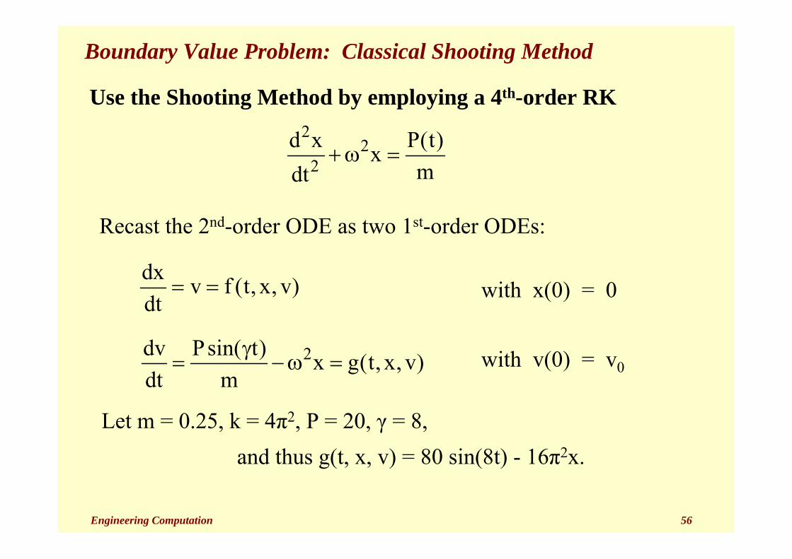
Boundary Value Problem: Classical Shooting Method
Use 4th-ord. RK Method to solve from t=0 until t=1 w/ h=0.1.1. Guess v(0) = 1.02. Find x(1) = 0.91687 (Note: not equal to 0.5)3. Guess v(0) = 1004. Find x(1) = 0.093325. Because our ODE is linear, we can always interpolate yields
the required initial value.
100 1.0v(0) (0.5 0.91687)0.09332 0.91687
−= − =
−51.113
6. With v(0) = 51.113, check for x(1) = 0.5000 OK

Engineering Computation 58
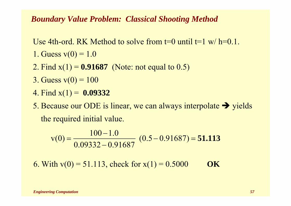
Finite Difference Method
• The shooting method is inefficient for higher-order equations with several boundary conditions.
• Finite Difference method has advantage of being direct (not iterative) for linear problems, but requires the solution of simultaneous algebraic equations.
• • • • • • •• •1 2 30 ii-1 i+1 nn+1. . .
xo x fΔx = h
x. . .
Engineering Computation 59
Finite Difference Method
Approach:1. Divide domain to obtain n interior discrete points
(usually evenly spaced @ h).2. Write a finite difference expression for the ODE at each
interior point.3. Use known values of y at x = xo and x = xf
4. Set up n linear equations with n unknowns. System is banded and often symmetric, so solve with an efficient method.
Note: If higher-order FDD equations and/or centered differences are used, you may need to employ imaginary or "phantom" points outside of domain to express B.C.'s (together with appropriate FD versions of B.C.'s).

Engineering Computation 60
Finite Difference Method
Sailboat mast deflection problem 4
4d v f (z)
EIdz= (Euler-Bernoulli Law of Bending)
at the base of mast: v(0) = 0; v'(0) = 0;at the top of mast: v''(L) = 0; v'''(L) = 0
where: E = Modulus of Elasticity (material property)I = Moment of Inertia (geometry of material)
f(z) = wind pressure at height zv(x) = deflection (displacement) from vertical
z = heightE I v'' = momentE I v''' = shear (applied force)

Engineering Computation 61
Finite Difference Method
Sailboat mast deflection problem: 4
4d v f (z)v
EIdz′′′′= =
at the base (z = 0): v(0) = 0; v'(0) = 0;at the top (z = L): v''(L) = 0; v'''(L) = 0
4i 2 i 1 i i 1 i 2
4 4d v v 4v 6v 4v vv ''''dx h
− − + +− + − += ≈
3i 2 i 1 i 1 i 2
3 3d v v 2v 2v vv '''dx 2h
− − + +− + − += ≈
2i 1 i i 1
2 2d v v 2v vv ''dx h
− +− += ≈
i 1 i 1dv v vv 'dx 2h
−− += ≈
[dist. load,f(z)]/EI
(shear)/EI
(bending moment)/EI
(slope)

Engineering Computation 62
Finite Difference Method
Sailboat mast deflection problem: 4
4d v f (z)
EIdz=
at the base: v(0) = 0; v'(0) = 0;at the top: v''(L) = 0; v'''(L) = 0
Mast with 11 Nodes
v(0)given
Use equation:
ImaginaryNode
Use v'(0) to get in terms
of v(1)
4
4d v f (z)
E Idz=
Imaginary Nodes
Use v''(L) = 0 to get in terms of v(9) & (10)
Use v'''(L) = 0 to get in terms
of other v's
0 1 2 3 4 5 6 7 8 9 10

Engineering Computation 63
Finite Difference Method
@ pt. i: vi-2 – 4 vi-1 + 6 vi – 4 vi+1 + vi+2 = h4 f(xi)/EI
Using h = L/10, write the FD equations at points 1, 2, 9 and 10:
@ i = 1 v-1 – 4 v0 + 6 v1 – 4 v2 + v3 = h4 f(x1)/EI (1)
@ i = 2 v0 – 4 v1 + 6 v2 – 4 v3 + v4 = h4 f(x2)/EI (2)
@ i = 9 v7 – 4 v8 + 6 v9 – 4 v10 + v11 = h4 f(x9)/EI (3)
@ i = 10 v8 – 4 v9 + 6 v10 – 4 v11 + v12 = h4 f(x10)/EI (4)
We now need to eliminate v–1, v0, v11, and v12
with the four boundary conditions
4
4d v f (z)
EIdz=

Engineering Computation 64
Finite Difference Method4
4d v f (z)
EIdz=
8 9 11 123
v 2v 2v v 02h
− + − +=
9 10 112
v 2v v 0h
− +=
1 1v v 02h
−− =
Eliminating v–1, v0, v11, and v12 with the four Boundary conditions
v(0) = 0: v0 = 0
v'(0) = 0: v-1 = v1
v''(L) = 0: v11 = 2v10 + v9
v'''(L) = 0: v12 = v8 - 4v9 + 4v10

Engineering Computation 65
Finite Difference Method4
4d v f (z)
EIdz= We substitute these into equations (1) to (4) to
eliminate the unknowns at the “imaginary” points
v0 = 0 v-1 = v1v11 = 2v10 + v9 v12 = v8 - 4v9 + 4v10
@ i = 1 7 v1 – 4 v2 + v3 = h4f(x1) / EI (1a)
@ i = 2 – 4 v1 + 6 v2 – 4 v3 + v4 = h4 f(x2)/ EI (2a)
@ i = 9 v7 – 4 v8 + 5 v9 – 2 v10 = h4f(x9) / EI (3a)
@ i = 10 v8 – 4 v9 + 2 v10 = h4f (x10)/ EI (4a)

Engineering Computation 66
Finite Difference Method
v f (x )1 1v f (x )2 2v f (x )3 3v f (x )4 4
4v f (x )5 5v f (x )6 6v f (x )7 7v f (x )8 8v f (x )9 9v10
7 -4 14 6 -4 1
1 4 6 4 11 -4 6 -4 1
1 -4 6 -4 1 h f1 -4 6 -4 1 EI
1 -4 6 -4 11 -4 6 -4 1
1 -4 5 -21 -4 2
⎧ ⎫⎡ ⎤⎪ ⎪⎢ ⎥− ⎪ ⎪⎢ ⎥
− − ⎪ ⎪⎢ ⎥⎪ ⎪⎢ ⎥⎪ ⎪⎢ ⎥⎪ ⎪⎢ ⎥ ⎪ ⎪ =⎨ ⎬⎢ ⎥⎪ ⎪⎢ ⎥⎪ ⎪⎢ ⎥⎪ ⎪⎢ ⎥⎪ ⎪⎢ ⎥⎪ ⎪⎢ ⎥⎪ ⎪⎢ ⎥
⎢ ⎥ ⎪ ⎪⎣ ⎦ ⎩ ⎭ f (x )10
⎧ ⎫⎪ ⎪⎪ ⎪⎪ ⎪⎪ ⎪⎪ ⎪⎪ ⎪⎪ ⎪⎨ ⎬⎪ ⎪⎪ ⎪⎪ ⎪⎪ ⎪⎪ ⎪⎪ ⎪⎪ ⎪⎩ ⎭

Engineering Computation 67
Finite Difference Method
Once we have solved for all the vi, we can obtain secondary results such as bending moments and shear forces by substitutingthe finite-divided-difference operators and the values of the viinto such equations as:
M = EI v''V = EI v'''
For more refined results, we can use a smaller h and more segments.

Engineering Computation 68
Merits of Different Numerical Methods for ODE Boundary Value Problems
• Shooting method
Conceptually simple and easy.Inefficient for higher-order systems w/ many boundary
conditions. May not converge for nonlinear problems.Can blow up for bad guess of initial conditions.
• Finite Difference methodStable Direct (not iterative) for linear problems.Requires solution of simultaneous algebraic eqns.More complex.
FD better suited for eigenvalue problems.

Engineering Computation 69
Engineering Applications of Eigenvalue ProblemsNatural periods and modes of vibration of structures and dynamical systems.
(C&C Ex. 27.4, p. 761)
Application: determination of the natural frequencies of a system
Example: A mass-spring system with three identical (frictionless) masses connected by three springs with different spring constants.
M M M
x1 x2 x33k 2k k
The displacement of each spring is measured relative to its own local coordinate system with an origin at the spring's equilibrium position.
21
1 1 22d xm 3kx 2k(x x )dt
= − − −2
22 1 2 32
d xm 2k(x x ) k(x x )dt
= − − − −2
33 22
d xm k(x x )dt
= − −

Engineering Computation 70
Engineering Applications of Eigenvalue Problems
If one assumes that x has the form:
xi = ai cos ω t ; d2x/dt2 = - ω2 ai cos ω t
Then, with λ = m ω2 / k , the governing equations become:
2
1 1 2 1 2 1m a 5a 2a 5a 2a a
kω
− = − + ==> − = λ
2
2 1 2 3 1 2 3 2m a 2a 3a a 2a 3a a a
kω
− = − + ==> − + − = λ
2
3 2 3 2 3 3m a a a a a a
kω
− = − ==> − + = λ

Engineering Computation 71
Engineering Applications of Eigenvalue Problems
1 2 1 1 1
1 2 3 2 2 2
1 2 3 3 3
5a 2a a 5 2 0 a a2a 32a a a 2 3 1 a a
a a a 0 1 1 a a
− = λ −⎡ ⎤ ⎧ ⎫ ⎧ ⎫⎪ ⎪ ⎪ ⎪⎢ ⎥− + − = λ ==> − − = λ⎨ ⎬ ⎨ ⎬⎢ ⎥ ⎪ ⎪ ⎪ ⎪− + = λ −⎣ ⎦ ⎩ ⎭ ⎩ ⎭
[A] {x} =λ {x}
1
2
3
5 2 0 aor 2 3 1 a 0
0 1 1 a
− λ −⎡ ⎤ ⎧ ⎫⎪ ⎪⎢ ⎥− − λ − =⎨ ⎬⎢ ⎥ ⎪ ⎪− − λ⎣ ⎦ ⎩ ⎭
[A – I λ] {x} = 0

Engineering Computation 72
Engineering Applications of Eigenvalue Problems
For a non-trivial solution:
det [A – I λ ] = 0 find5 2 0
det 2 3 1 00 1 1
− λ −⎡ ⎤⎢ ⎥− − λ − =⎢ ⎥− − λ⎣ ⎦
(5 – λ) [(3 – λ)(1 – λ) – (–1)(–1)] – 2 [(–1)(0) – (–2)(1 – λ)] = 0
(5 – λ) [2 – 4 λ + λ2] – 2 [ 2 – 2 λ] = 0
6 – 18 λ + 9 λ2 – λ3 = 0
The three solutions of the cubic equation are the three eigenvalues:
λ1 = 6.29 λ2 = 2.29 λ3 = 0.42
Fast oscillation Slow oscillation
The determinant yields a cubic equation for λ:

Engineering Computation 73
Engineering Applications of Eigenvalue Problems
i 1i
i 2i
i 3i
5 2 0 a2 3 1 a 0
0 1 1 a
− λ −⎡ ⎤ ⎧ ⎫⎪ ⎪⎢ ⎥− − λ − =⎨ ⎬⎢ ⎥ ⎪ ⎪− − λ⎣ ⎦ ⎩ ⎭
Because this is a homogeneous equation, we can only find the relative values of the ai's. For λ1 = 6.29
The corresponding eigenvectors {ai} are found by solving:
1i
2i
3i
5 6.29 2 0 a2 3 6.29 1 a 0
0 1 1 6.29 a
− −⎡ ⎤ ⎧ ⎫⎪ ⎪⎢ ⎥− − − =⎨ ⎬⎢ ⎥ ⎪ ⎪− −⎣ ⎦ ⎩ ⎭
2
1
a 0.645a
= − 3
1
a 0.122a
=

Engineering Computation 74
Engineering Applications of Eigenvalue Problems
Only the relative values of the ai's are significant. Thus setting a1 = 1.00 we have:
2
1
a 0.645a
= − 3
1
a 0.122a
=
{ }1
for = 6.29
1.000a 0.645
0.122
λ
⎧ ⎫⎪ ⎪= −⎨ ⎬⎪ ⎪⎩ ⎭
Fast
{ }
2
2
for = 2.29
0.74a 1.000
0.77
λ
⎧ ⎫⎪ ⎪= ⎨ ⎬⎪ ⎪−⎩ ⎭
{ }
2
2
for = 0.42
0.25a 0.55
1.000
λ
⎧ ⎫⎪ ⎪= ⎨ ⎬⎪ ⎪⎩ ⎭
Slow

Engineering Computation 75
Engineering Applications of Eigenvalue Problems
Thus, there are 3 possible natural frequencies.
Recall that the frequency is defined as
[A] {x} = λ {x}
[A – I λ] {x} = 0
det [A – I λ] = 0 ==> find λ
• If [A] is n x n, there are n eigenvalues λ iand n eigenvectors {x}i
• If [A] is symmetric, the eigenvectors are orthogonal:
kmλ
ω =
{x}iT {x}j = 0 if j ≠ i
= 1 if j = i

Engineering Computation 76
POWER METHOD for Eigenvector Analysis(An iterative approach for solving for eigenvalues & eigenvectors)
Assume that a vector {y} can be expressed as a linear combination of the eigenvectors:
{ }n
1 1 2 2 n n i ii 1
{y} = b {x } + b {x } + . . . + b {x } = b x=∑
Multiplying the above equation by [A] yields:
{ } { }n n
i i i i ii 1 i 1
[A] {y} = b [A] x = b x= =
λ∑ ∑Ordering the λ i so that | λ 1| > | λ 2| > | λ 3| > . . . > | λ n|
{ } { }n
i i1 1 1 i i
1 1i 2
Then [A] {y} = b x b x where 1=
⎛ ⎞⎛ ⎞λ λ⎜ ⎟λ + <⎜ ⎟⎜ ⎟λ λ⎝ ⎠⎝ ⎠∑

Engineering Computation 77
POWER METHOD for Eigenvector AnalysisMultiplying the equation by [A] again, we have:
Repeating this process m times:
{ } { }2n
22 i1 1 1 i i
1i 2
[A] {y} = b x b x =
⎛ ⎞⎛ ⎞λ⎜ ⎟λ + ⎜ ⎟λ⎜ ⎟⎝ ⎠⎝ ⎠∑
{ } { }mn
mm i1 1 1 i i
1i 2
[A] {y} = b x b x =
⎛ ⎞⎛ ⎞λ⎜ ⎟λ + ⎜ ⎟λ⎜ ⎟⎝ ⎠⎝ ⎠∑
i
1Since 0 for all i 1 as m ==> ,
⎛ ⎞λ==> ≠ ∞⎜ ⎟λ⎝ ⎠
then [A]m {y} λ1m b1{x1}
Since we can only know the relative values of the elements of {x}, we may normalize {x}. If {x} is normalized such that the largest element is equal to {1}, then is the first eigenvalue, λ1

Engineering Computation 78
POWER METHOD Numerical Example
Find the maximum eigenvector. Initial guess: {y}T = {1 1 1}
1 1
2 2
3 3
3 7 9 x x9 4 3 x x9 3 8 x x
⎡ ⎤ ⎧ ⎫ ⎧ ⎫⎪ ⎪ ⎪ ⎪⎢ ⎥ = λ⎨ ⎬ ⎨ ⎬⎢ ⎥⎪ ⎪ ⎪ ⎪⎢ ⎥⎣ ⎦ ⎩ ⎭ ⎩ ⎭
3 7 9 1 19 0.95[A]{y} 9 4 3 1 16 20 0.80
9 3 8 1 20 1.00
⎡ ⎤ ⎧ ⎫ ⎧ ⎫ ⎧ ⎫⎪ ⎪ ⎪ ⎪ ⎪ ⎪⎢ ⎥= = ==>⎨ ⎬ ⎨ ⎬ ⎨ ⎬⎢ ⎥⎪ ⎪ ⎪ ⎪ ⎪ ⎪⎢ ⎥⎣ ⎦ ⎩ ⎭ ⎩ ⎭ ⎩ ⎭
Approx. eigen-eigenvalue vector

Engineering Computation 79
POWER METHOD Numerical Example
Approximate error, εa:
23 7 9 0.95 0.92084
[A] {y} 9 4 3 0.80 18.95 0.778369 3 8 1.00 1.00
⎡ ⎤ ⎧ ⎫ ⎧ ⎫⎪ ⎪ ⎪ ⎪⎢ ⎥= =⎨ ⎬ ⎨ ⎬⎢ ⎥⎪ ⎪ ⎪ ⎪⎢ ⎥⎣ ⎦ ⎩ ⎭ ⎩ ⎭
2nd iteration
i, j i 1, j
j i, j
(e e 0.92084 0.95max *100% *100% 4.2%e 0.92084
−− −= =
33 7 9 0.92084 0.92420
[A] {y} 9 4 3 0.77836 18.623 0.773319 3 8 1.00 1.00
⎡ ⎤ ⎧ ⎫ ⎧ ⎫⎪ ⎪ ⎪ ⎪⎢ ⎥= =⎨ ⎬ ⎨ ⎬⎢ ⎥⎪ ⎪ ⎪ ⎪⎢ ⎥⎣ ⎦ ⎩ ⎭ ⎩ ⎭
3rd iteration
a0.92084 0.95 *100% 0.75%
0.92084−
ε = =

Engineering Computation 80
POWER METHOD Numerical Example
After 10 iterations:
0.92251{x} 0.77301
1.00
⎧ ⎫⎪ ⎪= ⎨ ⎬⎪ ⎪⎩ ⎭
a 0.00033%ε =18.622λ =

Engineering Computation 81
Engineering Applications of Eigenvalue Problems
1. Natural periods & modes of vibration of dynamic systems and structures. Boundary-value problem from separation of variables:
2
2 2y(x, t) ym a force m(x) k(x)
t x∂ ∂
∗ = ⇒ =∂ ∂
If one assumes y(x,t) = exp(iωt) u(x)
then displacement function u(x) satisfies ODE:
– ω2 u(x) = [k(x)/m(x)] d2u/dx2
which may be written: a(x) d2u/dx2 + ω2 u(x) = 0
With a FD approximation of u,xx = d2u/dx2 this becomes:
[A] {ui} = – ω2 {ui}

Engineering Computation 82
Engineering Applications of Eigenvalue Problems
2. Buckling loads and modes of structures (C&C 27.2.3, p. 762)
Deflection of vertically loaded beam with horizontally constrained end:
EI y'' – Py = 0; y(0) = 0; y(L) = 0.
Is there deflection?
3. Directions and values of principal stresses.
4. Directions and values of principal moments of inertia.
5. Condition numbers linear systems of equations.
6. Stability criteria for numerical solution of PDE’s.
7. Other problems in which "principal values" are sought.

Engineering Computation 83
Engineering Applications of Eigenvalue Problems
Matrix Form of Eigenvalue Problem
[A] {x} = λ {x}
( [A] – λ [I] ) {x} = 0 but want {x} ≠ 0
Computation of Eigenvalues and Eigenvectors
1. Power and Inverse Power method for largest and smallest eigenvalues. (C&C 27.2.5, p. 767)
2. Direct numerical algorithms: Jacobi, Given, Householder, and
QR factorization. (C&C 27.2.6, p. 770)
3. Use of characteristic polynomial for “toy” problems. (C&C 27.2.4, p. 765)

Engineering Computation 84
Engineering Applications of Eigenvalue Problems
Power Method for the largest Eigenvalue
Compute xt+1 = A xt / || xt ||
for larger and larger t to estimate largest λ(A).
Always works for Symmetric A.

Engineering Computation 85
Eigenvalue Problems: Power Method
Inverse Power Method for the smallest Eigenvalue
Compute xt+1 = B xt / || xt ||
for larger and larger t to estimate largest λ(B).
Here B = A-1. Eigenvalues of B are inverse of those of A.
BUT WE DO NOT COMPUTE A-1 ! (Don’t do it.)
Instead use LU decomposition of A.

Engineering Computation 86
Engineering Applications of Eigenvalue Problems
Shifting method for any Eigenvalue:
Suppose we want to compute eignvector whose eigenvalue is about δ.
Let B = (A – δ I)-1 and compute xt+1 = B xt / || xt ||
for larger and larger t to estimate largest λ[ (A – δ I) -1].
This will compute the eignvalue nearest to δ !But we DO NOT COMPUTE INVERSE. Use LU decomposition.
If A has eigenvector-value pairs (ei, λi),
(A – δ I) ei = A ei – δ I eI = λi ei– δ ei = ( λi – δ ) ei
Thus shifted matrix has same eignvectors ei as A with shifted eigenvalues ( λi – δ ).
Hence (A – δ I)-1 has eigenvalues ( λi – δ )-1.