Numerical Solution of Ordinary Differential Equationslya.fciencias.unam.mx/gfgf/pa20081/data/material/chap4_engineerin… · Numerical Solution of Ordinary Differential Equations

Numerical Solution of Ordinary Differential Equations

In this chapter we shall consider numerical solution of ordinary differential equations, ODEs. Here we will experience the real power of numerical analysis for engineering applications, as we will be able to tackle some real problems. We will consider both single and systems of differential equations. Since high- order ODEs can be converted to a system of first-order differential equations, our concentration will be on first-order ODEs. The extension to systems will be straightfonvard. We will consider al1 classes of ordinary differential equations: initial, boundary and eigenvalue problems. However, we will emphasize techniques for initial value problems because they are used extensively as the basis of methods for the other types of differential equations. The material in this chapter constitutes the core of this first course in numerical analysis; as we shall see in Chapter 5, numerical methods for partial differential equations are rooted in the methods for ODEs.

4.1 Initial Value Problems

Consider the first-order ordinary differential equation

We would like to find y( t ) for O < t 5 t f . The aim of al1 numerical methods for solution of this differential equation is to obtain the solution at time tn+l = tn + At, given the solution for O 5 t 5 tn. This process, of course, continues; i.e., once y,?+, = y(tn+,) is obtained, then yn+z is calculated and so on until the final time, i/.

We begin by considering the so-called Taylor series methods. Let's expand the solution at t,,,, about the solution at tn

h2 h3 111

~ h + l = yn +Ay; + -y: + zYn + 2

(4.2)

43

44 NUMERICAL SOLUTION OF ORDINARY DIFFERENTIAL EQUATIONS

where h = At. From the differential equation (4.1), we have

which can be substituted in the second term in (4.2). We can, in principle, stop at this point, drop the higher order terms in (4.2), and get a second-order approximation to y,+i using y,. To get higher order approximations to y,+, , we need to evaluate the higher order derivatives in (4.2) in terms of the known quantities at t = t,. We will use the chain rule to obtain

Since f is a known function of y and t, al1 the above partial derivatives can, in principle, be computed. However, it is clear that the number of terms increases rapidly, and the method is not very practica1 for higher than third order.

The ik thod based on the first two terms in the expansion is called the Euler method:

In using the Euler method, one simply starts from the initial condition, yo, and marches fonvard using this formula to obtain y,, y2,. . .. We will study the properties of this method extensively as it is a very simple method to analyze. From the Taylor series expansion it is apparent that the Euler method is second- order accurate for one time step. That is, if the exact solution is known at time step n, the numerical solution at time step n + 1 is second-order accurate. However, as with the quadrature formulas, in multi-step calculations, the errors accumulate, and the global error for advancing from the initial condition to the final time tf is only$rst-order accurate.

Among the more accurate methods that we will discuss are the Runge-Kutta formulas. With explicit Runge-Kutta methods the solution at time step t,+, is obtained in terms of y,, f (y,, t,), and f (y, t) evaluated at the intermediate steps between t, and t,+, = t, + At (not including t,+,). The higher accuracy is achieved because more information about f is provided due to the intermediate evaluations of f . This is in contrast to-the Taylor series method where we provided more information about f through the higher derivatives of f at t,.

wc mi the wh

Higher accuracy can also be obtained by providing information about f at times t < tn . That is, the corresponding formulas involve y,- 1 , y,-2, . . . , and fn-l, fn-2, . . . . These methods are called mtllti-step methods.

We will also distinguish between explicit and implicit methods. The preced- ing methods were al1 explicit. The formulas that involve f (y, t) evaluated at y ,+~ , tn+i belong to the class of implicit methods. Since f may be a non-linear function of y , to obtain the solution at each time step, implicit methods usually require solution of non-linear algebraic equations. Although the computational cost per time step is higher, implicit methods offer the advantage of numerical stability, which we shall discuss next.

4.2 Numerical Stability

So far, in the previous chapters, we have been concerned only with the accuracy of numerical methods and the work required to implement them. In this section the concept of numerical stability in numerical analysis is introduce4 which is a more critica1 property of numerical methods for solving differential equations. It is quite possible for the numerical solution to a differential equation to grow unbounded even though its exact solution is well behaved. Of course, there are cases for which the exact solution grows unbounded, but for our discussion of stability, we shall concentrate only on the cases in which the exact solution is bounded. Given a differential equation

Y' = f(y, t) (4.1)

and a numerical method, in stability analysis we seek the conditions in terms of the parameters of the numerical method (mainly the step size h ) for which the numerical solution remains bounded. In this context we have three classes of numerical methods:

Stable nzlmerical scheme: Numerical solution does not grow unbounded (blow up) with any choice of parameters such as the step size. We will have to see what the cost is for such robustness.

Unstable numerical scheme: Numerical solution blows up with any choice of parameters. Clearly, no matter how accurate they may be, such numerical schemes would not be useful.

Conditionall' stable: With certain choices of parameters the numerical solution remains bounded. Hopefully, the cost of the calculation does not become ~rohibitivel~ large.

would apply the so-called stability anabsis to a numerical method to deter- e its stability properties, i.e., to determine to which of the above categories

ethod belongs. The analysis is performed for a simpler equation than (4. l), ~ h h o ~ e f u l l ~ retains some of the features of the general equation. Consider

the two-dimensional Taylor series expansion of f (y, t):

Collecting only the linear terms and substituting in (4. l), we formally get

where A, al, a;! are constants. For example,

Discarding the non-linear terms (those involving higher powers of (y - yo), (t - to) or their product) on the right-hand side of (4.4) yields the linearization of (4.1) about (yo, to). For convenience and feasibility of analytical treatment, stability analysis is usually performed on the modelproblem, consisting of only the first term on the right-hand side of (4.4),

y' = Ay, (4.5)

instead of the general problem (4.1). Here, h is a constant. It turns out that the inhomogeneous terms in the linearized equation (4.4) do not significantly affect the results of the stability analysis. Note that the model equation has an exponential solution, which is the most dangerous part of the full solution of (4.1).

In our treatment of ( 4 9 , we will allow A to be complex

h = hR + ihz

with the real part hR 5 O to ensure that the solution does not grow with t. This generalization will allow us to readily apply the results of our analysis to systems of ordinary differential equations and partial differential equations. To illustrate this point, consider the second-order differential equation

The exact solution is sinusoidal

y = cl coswt + c2 sinot.

We can convert this second-order equation to two first-order equations

The eigenvalues of the 2 x 2 matrix A,

ar

le;

wl

wi. sol

4.3 STABlLlN ANALYSIS FOR 'THE EULER METHOD

1 : are h = f iw. Diagonalizing A with the matrix of its eigenvectors S,

I* leads to the uncoupled set of equations

I a

3 t

where

2' = Az,

1 " and A is the diagonal matrix with eigenvalues of A on the diagonal. The differ-

i ential equations for the components of z are

This simple example illustrates that higher order linear differential equations or systems of first-order linear differential equations can reduce to uncoupled ordinary differential equations of the form of (4.5) with complex coefficients. The imaginary part of the coefficient results in oscillatory solutions of the forrn e""', and the real part dictates whether the solution grows or decays. For our stability analysis we will be concerned onZy with cases where h has a zero or

u

negative real part. I

4.3 Stability Analysis for the Euler Method

Applying the Euler method (4.3),

Yn+i = Yn + h f (yn tn),

to the model problem (4.5) leads to

Yn+i = Yn + hhyn = yn(l + AA).

Thus, the solution at time step n can be written as

Yn = yo(1 + hh)n -

For complex h, we have

y, = yo(l + h ~ h + ihlh)" = yoon,

where a = (1 + hRh + i h I h ) is called the amplification factor. The numerical 01ution is stable (i.e., remains bounded as n becomes large) if

lol 5 l . (4.7)

Region of stability for the exact solution A Im(hh)

Figure 4.1 Stability diagram for the exact solution in the A R ~ - Alh plane.

Note that for hR 5 O (which is the only case we consider) the exact solution, yoeh', decays. That is, in the (hRh - hIh) plane, the region of stability of the exact solution is the left-hand plane as illustrated in Figure 4.1.

However, only a portion of this plane is the region of stability for the Euler method. This portion is inside the circle

For any value of hh in the left-hand plane and outside this circle the numerical solution blows up while the exact solution decays (see Figure 4.2). Thus, the Euler method is conditionally stable. To have a stable numerical solution, we must reduce the step size h so that hh falls within the circle. If h is real (and negative), then the maximum step size for stability is 2/)h(. That is, to get a stable solution, we must limit the step size to

Note that for real (and negative) A, (4.7) is enforced for hh as low as -2. The main consequence of this limitation on h is that it would require more time steps, and hence more work, to reach the final time of integration, t f . The circle (4.8)

Region of stability for Explicit Euler

Figure 4.2 Stability diagram for the explicit Euler method.

4.3 STABlLlTY ANALYSIS FOR THE EULER METHOD 49

is only tangent to the imaginary axis. Therefore, the Euler method is always unstable (irrespective of the step size) for pzirely imaginary h. If h is real and the numerical solution is unstable, then we must have

which means that (1 + hh) is negative with magnitude greater than 1. Since

the numerical solution exhibits oscillations with change of sign at every time A t e p . This oscillatory behavior of the numerical solution is usually a good indi-

cation of numerical instability.

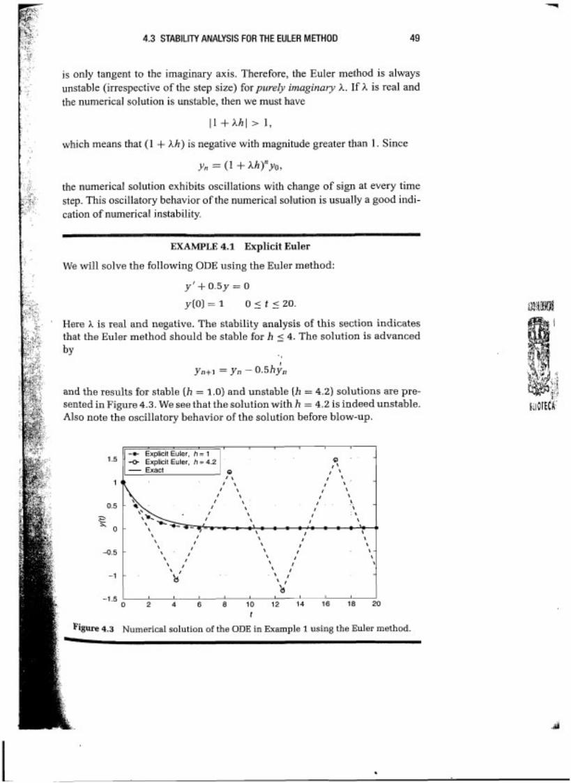
Ir EXAMPLE 4.1 Explicit Euler

l We will solve the following ODE using the Euler method:

y' + 0 . 5 ~ = O

y ( 0 ) = 1 O 5 t ( 20.

Here h is real and negative. The stability analysis of this section indicates that the Euler method should be stable for h 5 4. The solution is advanced

. ,

yn+i = yn - 0-5hj .n

and the results for stable (h = 1.0) and unstable (h = 4.2) solutions are presented in Figure 4.3. We see that the solution with h = 4.2 is indeed unstable. Also note the oscillatory behavior of the solution before blow-up.

3,

I

O 2 4 6 8 10 12 14 16 18 20 t

Figure 4.3 Numerical solution of the ODE in Example 1 using the Euler method.

O " - l \

Q 1 1

- -+ Explicit Euler, h = 1 -C+ Explicit Euler, h = 4.2 - Exact

\ 1 \ . \ I \

1 \ 1 1 \ 1

1 \ - 1

1 . \. \ \ 1

1 \ 1 : \ 1

1 * - - ; \ * * = * = = \ \ =

-0.5

-1

-1.5

\ \

\ 1

1

\ \ \

1 1

\ \ 1 \

- 1 \ / \ r . \ -

' 1 \ 1 \

1 1 \

\ 1 1 - . 'd . 1 -

\ I

'd 1 1 I 1 1 1 1 I I

NUMERICAL SOLUTION OF ORDINARY UIFFERENTIAL EQUATIONS

4.4 lmplicit or Backward Euler

The implicit Euler scheme is given by the following formula:

Note that in contrast to the exp1ici.t Euler, the implicit Euler does not allow us to easily obtain the solution at the next time step. If f is non-linear, we must solve a non-linear algebraic equation at each time step to obtain y,+¡, which usually requires an iterative algorithm. Therefore, the computational cost per time step for this scheme is, apparently, much higher than that for the explicit Euler. However, as we shall see below, the implicit Euler method has a much better stability property. Moreover, Section 4.7 will show that at each step, the requirement for an iterative algorithm may be avoided by the linearization technique.

Applying the backward Euler scheme to the model equation (4.5), we obtain

Solving for yn+l produces

where

Considering complex h, we have

The denominator is a complex number and can be written as the product of its modulus and phase factor,

where

For stability, the modulus of o must be less than or equal to 1; Le.,

4.5 IUUMERICAL ACCURACY REVlSlTED 51

This is always true because hR is negative and hence A > 1. Thus, the backward Euler scheme is unconditionally stable. Unconditional stability is the usual characteristic of implicit methods. However, the price is higher computational cost per time step for having to solve a non-linear equation.

It should be pointed out that one can construct conditionally stable implicit methods. Obviously, such methods are not very popular because of the higher cost per step without the benefit of unconditional stability. Also note that numerical stability does not necessarily imply accuracy. A method can be stable but inaccurate. From the stability point of view, our objective is to use the maximum step size h to reach the final destination at time t = t f . Large time steps translate to a lower number of finction evaluations and lower computational cost. Large time steps may not be optiinum for acceptable accuracy, but are strived for from the stability point of view.

EXAMPLE 4.2 Implicit (Backward) Euler

We now solve the ODE of Example 1 using the implicit Euler method. The stability analysis for the implicit Euler indicated that the numerical solution should be unconditionally stable. The solution is advanced by

and the results for h = 1.0 and h = 4.2 ar,b presented in Figure 4.4. Both solutions are now seen to be stable, as expected. The solution with h = 1.0 is more accurate. Note that the usual difficulty in obtaining the solution at each time step inherent with implicit methods is not encountered here because the differential equation in this example is linear.

t

4.5 Numerical Accuracy Revisited

ave shown that the numerical solution to the model problem

y' = Ay (4.5)

52 NLlMERlCAL SOLLITION CIF ORDINARY DIFFERENTIAL EQUATIONS

is of the form

Yn = yoan. (4.1 1 )

The exact solution is

In analogy with the modified wavenumber approach of Chapter 2, one can often determine the order of accuracy of a method by comparing the numerical and exact solutions for a model problem, i.e., (4.1 1) and (4.12). That is, we compare the amplification factor a with

For example, the amplification factor of the explicit Euler is

and the amplification factor for the backward Euler is

Thus, both methods are able to reproduce only up to the hh term in the exponential expansion. Each method is second-order accurate for one time step, but globally first order. From now on, we will cal1 a method a th order if its amplification factor matches al1 the terms up to and including the hah'"/a!! term in the exponential expansion. The order of accuracy derived in this manner from the linear analysis (i.e., from application to (4.5)) should be viewed as the upper limit on the order of accuracy. A method may have a lower order of accuracy for non-linear equations.

Often the order of accuracy by itself is not very informative. In particular, in problems with oscillatory solutions, one is interested in the phase and amplitude errors separately. To understand this type of error analysis, we will consider the model equation with pure imaginary A:

The exact solution is e'"', which is oscillatory. The frequency of oscillations is o and its amplitude is 1. The numerical solution with the explicit Euler is

where a = 1 + ioh. It is clear that the amplitude of the numerical solution,

is greater than 1, which reconfirms that the Euler method is unstable for purely imaginary h. o is a complex number and can be written as

! 4.6 TRAPEZOIDAL METHOD

Phase lag

iC):

f , Figure 4.5 A schematic showing the arnplitude and phase errors in the numerical solution.

where

1 1 lm\a) e = tan- o h = tan- - Re(a) '

f A measure of the phase error (PE) (see Figure 4.5) is obtained from comparison ;: with the phase of the exact solution

P E = wh - 0 = o h - tan-'wh.

the power series

tan-' /.rh

1

for tan- ' , (oh13 (wh)' (wh

- h - - A- - - -

1 which corresponds to a phase lag. This is the phase error encountered at each ! Step. The phase error after n time steps is nPE.

4.6 Trapezoidal Method

e formal solution to the differential equation (4.1) with the condition y(&) =

t

Y@) = Yn + f (y, tf)dtf .

Yn+i =yn + [+' f (y, tf) dtf .

Approximating the integral with the trapezoidal method leads to

h yn+i = yn + 2 [ f ( ~ n + ~ . tn+l) + f(y.7 tn)I. (4.14)

This is the trapezoidal method for the solution of ordinary differential equations. When applied to certain partial differential equations it is often called the Crank- Nicolson method. Clearly the trapezoidal method is an implicit scheme.

Applying the trapezoidal method to the model equation yields

Expanding the amplification factor o leads to

which indicates that the method is second-order accurate. The extra accuracy is obtained at virtually no extra cost over the backward Euler method.

Now, we will examine the stability properties of the trapezoidal method by computing the modulus of o for complex h =' hR + ihr. The amplification factor becomes

Both the numerator and denominator are complex and can be written as Aeie and Beia, respectively, where

and

Thus,

4.6 TRAPEZOIDAL METHOD 55

Since we are only interested in cases where hR < 0, and for these cases A < B,

la( < l .

Thus, the trapezoidal method is unconditionally stable, which is expected since it is an implicit method. Note, however, that for real and negative A,

lim o = -1, h 4 o o

which implies that for large time steps, the numerical solution onyo oscillates between yo and -yo from one time step to the next, but the solution will not

Let us examine the accuracy of the trapezoidal method for oscillatory solutions, h = iw. In this case (AR = O), A = B, and

1 0 1 = l.

Thus, there is no amplitude error associated with the trapezoidal method. Since

o = e 2ie 6 = tan-' (T) , the phase error is given by

wh P E = o h - 2 t a n - 1 = w h - 2 ... =-+ . . . 2 [ "213 1 'y":'

which is about four times better than that for the explicit Euler but of the same

EXAMPLE 4.3 A Second-Order Equation

We now consider the second-order equation

y"+wZy=O t > O

y (01 = yo ~ ' ( 0 ) = 0,

and investigate the numerical solutions by the explicit Euler, implicit Eu- ler, and trapezoidal methods. In Section 4.2 it was dernonstrated how this equation could be reduced to a coupled pair of first-ordw equations:

2 y ; = y2 y; = -o y1.

[; 1' = [-"o Z ] [Y: .] . en decoupled, giving

z í = iwzl z2 = -ioz2.

e stability of the numerical solution depends upon the eigenvalues i w d -io that decouple the system. We see that here the eigenvalues are

I . . lmplicit Euler I Trapezoidal

Exact

Figure 4.6 Numerical solution of the ODE in Example 3.

imaginary and therefore predict the Euler solution to be unconditionally unstable. We have also seen that both backward Euler and trapezoidal methods are unconditionally stable. We will show this to be the case by numerical simulation of the equations. Solution advancement proceeds as follows. For explicit Euler:

t

For implicit Euler:

For trapezoidal:

[ : h 2 -.] [y:] n + l = [ -w lZh 5 4 1 [Y'] Y2 n

Numerical results are plotted in Figure 4.6 for y, = 1, w = 4, and time step h = 0.15.

We see that the explicit Euler rapidly blows up as expected. The implicit Euler is stable, but decays very rapidly. The trapezoidal method performs the best and has zero amplitude error as predicted in the analysis of Section 4.6; however, its phase error is evident and is increasing as the solution proceeds.

Although the numerical methods used in the previous example were introduced in the context of a single differential equation, their application to a system was a straightfonvard generalization of the corresponding single equation formulas. It is also important to emphasize that the decoupling of the equations using eigenvalues and eigenvectors was performed solely for the purpose of stability analysis. The equations are never decoupled in actual numerical solutions.

4.7 LlNEARiZATlON FOR IMPLlClT METHODS

4.7 Linearization for lmplicit Methods

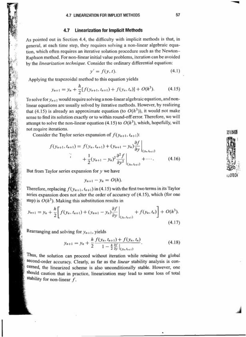
As pointed out in Section 4.4, the difficulty with implicit methods is that, in general, at each time step, they requires solving a non-linear algebraic equation, which often requires an iterative solution procedure such as the Newton- Raphson method. For non-linear initial value problems, iteration can be avoided by the linearization technique. Consider the ordinary differential equation:

Y' = f(y7 t). (4.1)

Applying the trapezoidal method to this equation yields h

Yn+i = Yn + Z [ f ( ~ n + i , tfi+i) + f(yn, tn)] + 0(h3). (4.15)

To solve f ~ r y , + ~ would require solving a non-linear algebraic equation, and non- linear equations are usually solved by iterative methods. However, by realizing that (4.15) is already an approximate equation (to 0(h3)), it would not make sense to find its solution exactly or to within round-off error. Therefore, we will attempt to solve the non-linear equation (4.15) to 0(h3), which, hopefully, will not require iterations.

Consider the Taylor series expansion of f (yn+17 tn+l):

f ( ~ n + i 7 tn+i) = f ( ~ n 7 tn+i) + ( ~ n + i - ~ n ) - . ,

l ay ( y n . t n + i )

I + 2(yn+1 1 - Yn)'-ii/ 1 + - (4.1 6)

ay ( , . tn+ l )

But from Taylor series expansion for y we have

Yn+i - Yn = O(h).

Therefore, replacing f (y,+i, tn+i) in (4.15) with the first two terms in its Taylor series expansion does not alter the order of accuracy of (4.15), which (for one step) is O(h3). Making this substitution results in

[ " 1 +f(yn, tn) l+0(h3)- n + l = Y n + 5 f(yn, tn+i) f (yn+i -Y,)-

'Y ( f i ? t n + i )

(4.1 7)

Rearranging and solving for yn+i7 yields

h f(yn7tn+i) + f ( ~ n , t n ) Yn+i = Yn + - h af

(4.18) 2 1- - -1

2 ay ( y n , t , , + i )

bus, the solution can proceed without iteration while retaining the global econd-order accuracy. Clearly, as far as the linear stability analysis is con- eme4 the linearized scheme is also unconditionally stable. However, one hould caution that in practice, linearization may lead to some loss of total tability for non-linear f .

EXAMPLE 4.4 Linearization

We consider the non-linear ordinary differential equation

and its numerical solution by the trapezoidal method:

This, of course, is a non-linear algebraic equation for yn+l. Using the linearization method developed in this section, where f is now y (y - l), we arrive at the following linearized trapezoidal method:

Since the non-linearity is quadratic, we may also solve the resulting non- linear algebraic equation directly and compare the direct implicit solution with the linearized solution. The direct implicit solution is given by

These equations were advanced from time t = O to t = 1. The error in the solution at t = 1 is plotted in Figure 4.7 versiis the number of steps taken. The slopes for both the trapezoidal and linearized trapezoidal methods clearly show a second-order dependence upon number of steps, demonstrating that second-order accuracy is maintained with linearization. The directly solved trapezoidal method is slightly more accurate, but this is a problem-specific phenomenon (for example, the linearized trapezoidal solution for y ' + y ' = O yields the exact solution for any h while the accuracy of the direct implicit solution is dependent on h).

. . T . .. - Trapezoidal - Linearized Trapezoidal

1 0 ' ~ - l

1 o0 101 18 1 o3 N -- Nurnber of Steps

Figure 4.7 Error in the solution of the ODE in Example 4.

4.8 RUNGE-KUllA METHODS

4.8 Runge-Kutta Methods

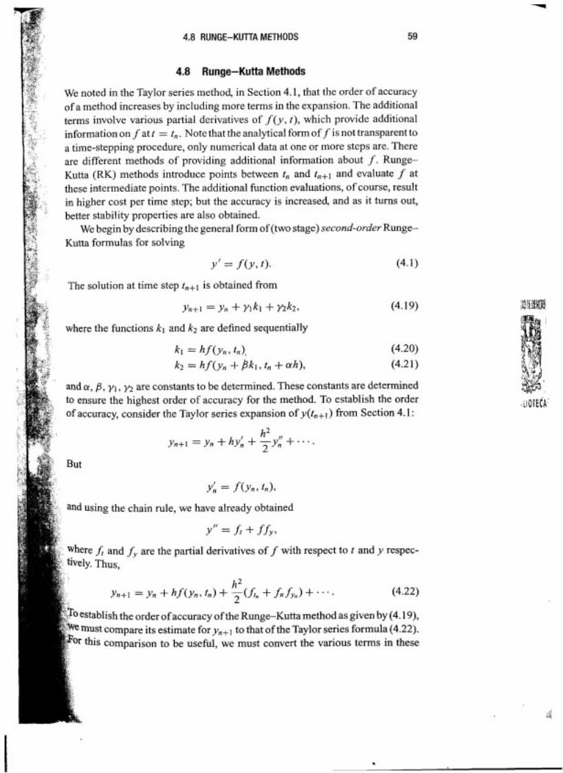
We noted in the Taylor series method, in Section 4.1, that the order of accuracy of a method increases by including more terms in the expansion. The additional terms involve various partial derivatives of f (y, t), which provide additional information on f at t = t, . Note that the analytical form of f is not transparent to a time-stepping procedure, only numerical data at one or more steps are. There are different methods of providing additional information about f . Runge- Kutta (RK) methods introduce points between tn and t,+~ and evaluate f at these intermediate points. The additional function evaluations, of course, result in higher cost per time step; but the accuracy is increased, and as it turns out, better stability properties are also obtained.

We begin by describing the general form of (two stage) second-order Runge- Kutta formulas for solving

The solution at time step t,+l is obtained from

where the functions kl and k2 are defined sequentially

anda, /3, yl , y2 are constants to be determined. These constants are determined to ensure the highest order of accuracy for the method. To establish the order of accuracy, consider the Taylor series expansion of y(tn+,) from Section 4.1:

Y:, = f (Y, 7 tn),

and using the chain rule, we have already obtained

y" = ft + ffr, where f, and f, are the partial derivatives of f with respect to t and y respec-

h2 Yn+i = Y n + h f ( ~ n , f n ) + + f n f f i ) f (4.22)

the order of accuracy of the Runge-Kuttamethod as given by (4.19), pare its estimate for y,+, to that of the Taylor series formula (4.22).

this comparison to be usehl, we must convert the various terms in these


expressions into common forms. Two-dimensional Taylor series expansion of k2 (4.21) leads to

Noting that kl = h f (y,, tn,) and substituting in (4.19) yields

Comparison of (4.22) and (4.23) and matching coefficients of similar terms leads to

These are three non-linear equations for the four unknowns. Using a as a free parameter, we have

With three out of the four constants chosen, we have a one-paramqter family of second-order Runge-Kutta formulas:

k2 = h f ( y n + a k i , tn + ah ) (4.24b)

Thus, we have a second-order Runge-Kutta formula for each value of a chosen. The choice a = 112 is made frequently. In actual computations, one calculates k l using (4.24a); this value is then used to compute k2 using (4.24b) followed by the calculation of yn+1 using (4.24~).

Runge-Kutta formulas are often presented in a different but equivalent form. For example, the popular forrn of the second-order Runge-Kutta formula ( a = 112) is presented in the following (predictor-corrector) format:

Here, one'calculates thepredicted value in (4.25a) which is then used in (4.25b) to obtain the corrected value, yn+l.

4.8 RUNGE-KUTTA METHODS 61

. Now, let's use linear analysis to gain insight into the stability and accuracy of the second order Runge-Kutta method discussed above. Applying the Runge- Kutta method in (4.24) to the model equation y' = Ay results in

k* = hhy,

k2 = h(hyn + ah2hyn) = hh(1 + ahh)yn

Thus, we have a confirmation that the method is second-order accurate. For stability, we must have la 1 ( 1, where

A convenient way to obtain the stability boundary, i.e., lo 1 = 1, of the method

and find the complex roots hh of this polynomial for different values of 8. Recall that \eie 1 = 1 for al1 values of 8 . The resulting stability region is shown in Figure 4.8. On the real axis the stability boundary is the same as that of explicit Euler ( ( A R h ( 5 2); however, there is significant improvement for complex h. The method is also unstable for purely imaginary h. In this case, substituting h = i o into (4.27) results in

i.e., the method is unconditionally unstable for purely imaginary h. However, note that for small values of wh, this method is less unstable than explicit Euler.

Let's consider numerical solution of

~ i n g the explicit Euler method and a second-order Runge-Kutta scheme. ose the differential equation is integrated for 100 time steps with 0.2; that is, the integration time is from t = Oto t = 20/w. Each numerical

62 NLlNlERlCAL SOLUTION OF ORDINARY DlFFERENTlAL EQUATIONS

solution after 100 time steps can be written as a 100 y = y o ,

where a is the corresponding amplification factor for each method. For the Euler scheme, la 1 = 4- = 1.0198, and for the RK method, from (4.28), we have la1 = 1.0002. Thus, after 100 time steps, for the RK method we have y = 1.02, i.e., there is only 2% amplitude error, whereas for the Euler method we have y = 7.10!

The phase error for the second-order RK scheme is easily calculated from the real and imaginary parts of a for the case h = iw:

But

w2h2 w4h4 t a n ( = wh (1 + +--+...

1 - - 4

Hence,

which is only a factor of 2 better than Euler, but of opposite sign. Negative phase error corresponds to phase lead (see Example 6).

The most widely used Runge-Kutta method is the fourth-order formula. This is perhaps the most popular numerical scheme for initial value problems. The fourth-order formula can be presented in a typical RK format:

where

4.8 RUNGE-KUTTA ME'THODS

Figure 4.8 Stability diagrams for second- and fourth-order Runge-Kutta methods.

I

Note that four function evaluations &e required at each time step. Applying the method to the model equation, y ' = Ay, leads to

L O

"'i i which confirms the fourth-order accuracy of the method. Again, the stability di-

agram is obtained by finding the roots of the following fourth-order polynomial & t with com~lex coefficients:

r different values of O 5 0 5 n. This requires a root-finder for polynomials ith complex coefficients. The resulting region of stability (Figure 4.8) shows a

ignificant improvement over that obtained by the second-order Runge-Kutta. Particular, it has a large stability region on the imaginary axis. In fact there

e two small stable regions corresponding to positive Re@), where the exact lution actually grows; that is, the method is artificially stable for the parameters rresponding to these regions.


EXAMPLE 4.6 Runge-Kutta

We solve the problem of Example 3 using second- and fourth-order Runge- Kutta algorithms. The details for the second-order Runge-Kutta advancement are

Fourth-order Runge-Kutta advancement proceeds similarly. Again numerical results are plotted in Figure 4.9 for y, = 1, u = 4, and time step h = 0.15.

- - - - - .. . .*. ..

. . . . . . . . . Exact . .. ... .. .:. . . . . . . . :. . .. . . . . ... . . . .. . . . . . .

Figure 4.9 Numerical solution of the ODE in Example 3 using Runge-Kutta methods.

It can be seen that the second-order scheme is mildly unstable as predicted by the linear stability analysis. The fourth-order Runge-Kutta solution is stable as predicted and is highly accurate, showing to plotting accuracy, virtually no phase or amplitude errors.

The most expensive part of numerical solution of ordinary differential equations is the function evaluations. The number of steps (or the step size h ) required to reach the final integration time t f is therefore directly related to the cost of the computation. Hence, both the stability characteristics and the accuracy come into play in establishing the cost-effectiveness of a numerical method. The fourth-order Runge-Kutta scheme requires four function evaluations per time step. However, it also has superior stability as well as excellent accuracy properties. These characteristics, together with its ease of programming, have made the fourth-order RK one of the most popular schemes for the solution of ordinary and partial differential equations.

4.9 MULTI-STEP METHODS 65

Finally, note that the order of accuracy of the second- and fourth-order Runge-Kutta formulas, discussed in this section, also corresponded to their respective number of function evaluations (stages). It turns out that this trend does not continue beyond fourth order. For example, a fifth-order Runge-Kutta formula requires six function evaluations.

4.9 Mi.ilti-Step Methods

The Runge-Kutta formulas obtained higher order accuracy through the use of severa1 function evaluations. However, higher order accuracy can also be achieved by using data from prior to t,,; that is, if the solution andlor f at tn-, , tn-2, . . are used. This is another way of providing additional information about f . Methods that use information from prior to step n are called multi- step schemes. The apparent price for the higher order of accuracy is the use of additional computer memory, which can be of concern for partial differential equations, as discussed in Chapter 5. Multi-step methods are not self-starting. Usually another method such as the explicit Euler is used to start the calculations for the first or the first few time steps.

A classical multi-step method is the leapfrog method:

~ n + i = yn-I + 2hf (Y,, tn) + 0(h3). (4.32)

This rnethod is derived by applying the second-order central difference formula for y ' in (4.1). Thus, the leapfrog method is a second-order method. Starting with an initial condition yo, a self-starting method like Euler is used to obtain yl, and then leapfrog is used for steps two and higher. Applying leapfrog to the model equation, y ' = Ay, leads to

Yn+i - Yn-i = 2hhyn.

This is a difference equation for y, that cannot be solved as readily as the schemes discussed up to this point. To solve it, we assume a solution of the

Y n = onyo.

Substitution in the difference equation leads to

an+l - = 2hhon.

Dividing by a"-' , we will get a quadratic equation for o

o2 - 2hho - 1 = 0,

ich can be solved to yield

o1,2 = I h i- ,/m.


Having more than one root is the key characteristic of multi-step methods. For comparison with the exponential solution to the model problem, we expand the roots in powers of hh

The first root shows that the method is second-order accurate. The second root is spurious and often is a source of numerical problems. Note that even for h = 0, the spurious root is not equal to l . It is also apparent that for h real and negative, the spurious root has a magnitude greater than 1 which leads to instability.

Since the difference equation for y, is linear, its general solution can be written as a linear combination of the roots, i.e.,

That is, the solution is composed of contributions from both physical and spurious roots. The constants cl and c2 are obtained from the starting conditions yo and y1 by letting n = O and n = 1, respectively, in (4.33):

Solving for cl and c~ leads to . , 1

C1 = Y i - Y002 0lY0 - Y1 C2 =

01 - 0 2 01 - 0 2

Thus, for the model problem, if we choose y1 = olyo, the spurious root is completely suppressed. In general, we can expect the starting scheme to play a role in determining the leve1 of contribution of the spurious root. Even if the spurious root is suppressed initially, round-off errors will restart it again, In the case of leapfrog, the spurious root leads to oscillations from one step to the next.

Application of leapfrog to the case where h = iw is pure imaginary leads to

01,~ = i o h & Jq. If (wh( 5 1, then

In this case leapfrog has no amplitude error. This is the main reason for the use of leapfrog method. If (wh ( > 1, then

and the method is unstable. Finally, we present the widely used second-order Adams-Bashforth method.

This method can be easily derived by using the Taylor series expansion of :

4.9 MULTI-STEP METHODS

Substituting

and a first-order finite difference approximation for y{

Thus, the Adams-Bashforth method is second-order accurate globally. Ap-

, , plying the method to the model problem leads to the following second-order

& difference equation for y, :

?,

Once again assuming solutions of the form yn = o" results in a quadratic equa- with roots

Using the power series expansion for the square root

9 2

h2hh') - ; (hh + ?h2h2)

The spurious root for the Adams-Bashforth method appears to be less gerous. Observe that it approaches zero if h + O. The stability region of

e Adams-~ashforth method is shown in Figure 4.10. It is oval-shaped in the h - hIh plane. It crosses the real axis at - 1, which is more limiting than the plicit Euler and second-order Runge-Kutta methods. It is also only tangent to

imaginary axis. Thus, strictly speaking, it is unstable for pure imaginary A,

-'.O 1 Figure 4.10 Stability diagram for the second-order Adams-Bashforth method.

but it turns out that the instability is very mild. For example, if we use Adams- Bashforth in the problem discussed in Example 5, we obtain la1 1'0° = 1.04, which is only slightly worse than the second-order Runge-Kutta.

-- -

f W EXAMPLE 4.7 Multi-Step Methods

fu We solve the problem of Example 3 with the leapfrog and Adams-Bashforth multi-step methods. The details for the leapfrog advancement are given as

2 n = y;-' - 2ho y, .

Implementation of the second-order Adams-Bashforth is similar. These multi-step methods are not self-starting and require a single step method to calculate the first time level. Explicit Euler was chosen for the start-up. Once again, numerical results are plotted in Figure 4.11 for y, = 1, o = 4,

and time step h = 0.15. We see that the leapfrog method is stable and with very little ampli-

tude error. There is a slight amplitude error attributed to the explicit Eu- ler calculation for the first time level. This error is not increased by the leapfrog advancement as predicted by our analysis of the model problem. The phase error for leapfrog is seen to be Significant and increasing with time. Adams-Bashforth gives a slowly growing numerical solution, which is expected as it is mildly unstable for al1 problems with purely imaginary eigenvalues.

?! 4.10 SYSTEM OF FIRST-ORDER ORDINARY DIFFERENTIAL EQUATIONS 69

Figure 4.11 Nurnerical solution of the ODE in Exarnple 3 using rnulti-step methods.

4.1 0 Systern of First-Order Ordinary Differential Equations

Recall that a higher order ordinary differential equations can be converted to a system of first-order ODEs. Systems of ODEs also naturally appear in many

z , . physical situations such as chemical reactions among severa1 species or vibra- tion of a complex structure with severa1 elements. A system of ODEs can be written in the generic form

where y is a ;ector with elements y, and f ( y i , y*, y j , . . . , yni , t ) is a vector function with elements J ; ( y l , y2, y3, . . . , ym , t), i = 1,2, . . . , m.

From the applications point of view, numerical solution of a system of ODEs, is a straightfonvard extension of the techniques used for a single ODE. For example, application of the explicit Euler to (4.35) yields

The right-hand side can be calculated using data from the previous time step and each equation can be advanced fonvard.

From the conceptual point of view, there is only one fundamental difference between numerical solution of one ODE and that of a system. This is the stiffness Property that leads to some numerical problems in systems, but it is not an issue With a single ODE. We shall discuss stiffness in connection with the system of equations with constant coefficients

Where A is an m x m constant matrix. Equation (4.36) is the model problem for SYstems of ODEs. In the same manner that the model equation was helpful in aalyzing numerical methods for a single ODE, (4.36) is useful for analyzing numerical methods for systems. From linear algebra we know that this system will have a bounded solution if al1 the eigenvalues of A have negative real parts.

This is analogous to the single-equation model problem, y ' = Ay, where the real part of h was negative. Applying the Euler method to (4.36) leads to

To have a bounded numerical solution, the matrix Bn = (1 + h A)n should approach zero for large n. A very important result from linear algebra states:

The powers of a matrix approach zero for large values of the ex- ponent if the moduli of its eigenvalues are less than 1. That is, if C is a matrix and the moduli of its eigenvalues are less than 1, then

lim Cn -+ O. n - + w

Therefore, the magnitudes of the eigenvalues of B must be less than 1. The eigenvalues of B are

where hi are the eigenvalues of the matrix A . Thus, for numerical stability, we must have

The eigenvalue with the largest modulus places the most restriction on h. If the eigenvalues are real (and negative), then

If the range of the magnitudes of the eigenvalues is large (JhlmaX/JhJmin » 1) and the solution is desired over a large span of the independent variable t, then the system of differential equations is called a stiffsystem. Stifiess arises in physical situations with many degrees of freedom but with widely different rates of responses. Examples include a system composed of two springs, one very stiff and the other very flexible; a mixture of chemical species with very different reaction rates; and a boundary layer (with two disparate length scales).

Stiff systems are associated with numerical difficulties. Problems arise if the system of equations is to be integrated to large values of the independent variable t. Since the step size is limited by -the part of the solution with the "fastest" response time (Le., with the largest eigenvalue magnitude), the number of steps required can become enormous. In other words, even if one is interested only in the long-term behavior of the solution, the time step must still be very

4.10 SYSTEM OF FIRST-ORDER ORDINARY DIFFERENTIAL EQUATIONS 71

small. In practice, to circumvent stiffness, implicit methods are used. With implicit methods there is no restriction on the time step due to numerical stability. For high accuracy, one can choose small time steps to resolve the rapidly varying portions of the solution (fast parts) and large time steps in the slowly varying portions. There are stiff ODE solvkrs (such as Nt~merical Recipes' S tif b s , MATLAB's ode2 3 S, or 1 sode*) that have an adaptive time-step selection mechanism. These are based on implicit methods and automatically reduce or increase the time step depending on the behavior of the solution. Note that with explicit methods one cannot use large time steps in the slowly varying part of the solution. Round-off error will trigger numerical instability associated with the fast part of the solution, even if it is not a significant part of the solution during any portion of the integration period.

EXAMPLE 4.8 A Stiff System (Byrne and Hindmarsh)

The following pair of coupled equations models a ruby laser oscillator

d n - d t - - -n(@ +B1+ Y

- = $ [ p n - u) + ~ ( 1 + nl d t

a = 1.5 x 10-l8 B = 2.5 x y = 2.1 x p = 0.6 a = 0.18 t = 0.016

n ( O ) = - 1 @ ( 0 ) = 0 .

The variable n represents the population inversion and the variable $ repre- nts the photon density. This problem is known to be stiff. We will compare e performance of a stiff equation solution package ( l s o d e ) with a standard urth-order Runge-Kutta algorithm. The solution using l s o d e is plotted in igures 4.12 and 4.13.

Solving the same problem to roughly the same accuracy using a fourth- der Runge-Kutta routine required about 6 0 times more computer time an the stiff solver. We were unable to use large time steps to improve

solution because stability is limited by the quickly varying modes in the tion even when they are not very active. The eigenvalue with the highest

gnitude still dictates the stability limit even when the modes supported the smaller eigenvalues are dominating the solution.

ailable on the World Wide Web; check for example, http: / /www. n e t l i b . orgl.

NUMERICAL SOLUI'ION OF ORDINARY DIFFERENTIAL EQUATIONS

0.5 Y 1

Time

Figure 4.12 Numerical solution of the ODE system in Example 8 using lsode.

. . . . . . . . . . . .

. . . . . . . . . . . . . . . . . .

O 1e+05 2e+05 3e+05 4e+05 5e+05 6e+05 7e+05 Time

Figure 4.13 Numerical solution of the ODE system in Example 8 using lsode.

We have pointed out that the difficulty with implicit methods is that, in general, at each time step, they require solving a non-linear algebraic equation that often requires an iterative solution procedure such as the Newton-Raphson method. It was shown in Section 4.7 that for a single non-linear differential equation, iteration can be avoided by the Iinearization technique. Linearization can also be applied in conjunction with application of implicit methods to a system of ODEs. Consider the system

where bold letters are used for vectors. Applying the trapezoidal method results in

4.1 1 BOUNDARY VALUE PROBLEMS 73

We would like to linearize f (u("+'), tn+i). Taylor series expansion of the elements of f denoted by f; yields

ni

We can write this in matrix form as follows:

is the Jacobian matrix. We now substitute this linearization of f (U("+'), tn+]) into (4.37). It can be seen that, at each time step, instead of solving a non-linear systern of algebraic equations, we would sblve the following system of linear

;. algebraic equations:

: Note that the matrix A is not constant (its elements are functions of t) and should ' be updated at every time step. 8 $3 L i

1 4.1 1 Boundary Value Problems b

When data associated with a differential equation are prescribed at more than one value of the independent variable, then the problem is a boundary value problem. ln initial value problems al1 the data (y(O), yf(0), . . .) are prescribed at one value of the independent variable (in this case at t = O). To have a boundary value problem, we must have at least a second-order differential equation

U where f is an arbitrary function. Note that here the data are prescribed at x = O

and at x = L. The same differential equation, together with data y(0) = yo and ~ ' ( 0 ) = y,, would be an initial value problem.

l- There are two techniques for solving boundary value problems: 8' f l. Shooting method Shooting is an iterative technique which uses the standard

methods for initial value problems such as Runge-Kutta methods.

74 IUUMERICAL SOLUTION OF ORDINARY DIFFERENTIAL EQUATIONS

2 . Direct Methods. These methods are based on straightforward finite- differencing of the derivatives in the differential equation and solving the resulting system of algebraic equations.

We shall begin with the discussion of the shooting method.

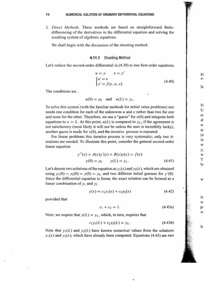
4.1 1.1 ~hoot ing Method

Let's reduce the second-order differential in (4.39) to two first-order equations

The conditions are , \

u(0) = yo and u(L) = y~ .

To solve this systei (with the familiar rnethods for initial value problems) one needs one condition for each of the unknowns u and v rather than two for one and none for the other. The~;efore, we use a "guess" for v(0) and integrate both equations to x = L. At this point, u(L) is compared to y ~ ; if the agreement is not satisfactory (most likely it will not be unless the user is incredibly lucky), another guess is mahe for v(O), and the iterative process is repeated.

For linear problems this iterative process is very systematic; only two iterations are needed. To illustrate this point, consider the general second-order linear equation

Let's denote two solutions of the equation as y1 (x) and y2(x), which are obtained using yl(0) = y2(0) = y(0) = yo, and two different initial guesses for y'(0). Since the differential equation is linear, the exact solution can be formed as a linear combination of y l and y2

provided that

Next, we require that y(L) = y ~ , which, in turn, requires that

Note that yl(L) and y2(L) have known numerical values from the solutions yi(x) and y2(x), which have already been computed. Equations (4.43) are two

4.1 1 BOUNDARY VALUE PROBLEMS

Y(L)A

1 1 1 1 1 1 1 1 1 -

Y; (0) Y; (0) Y; (0) Y' @)

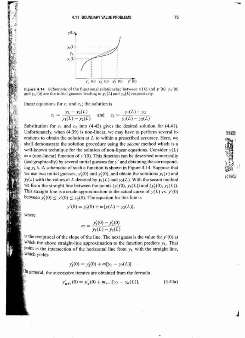
Figure 4.14 Schematic of the functional relationship between y (L) and ~ ' ( 0 ) . y1 '(0) and y, ' ( O ) are the initial guesses leading to yl (L) and yz(L) respectively.

ar equations for cl and c2; the solution is

C] = YL - y2(L) and c2 = Yl(Q - YL

YI(L) - Y2(L) ydL) - y2(L)'

stitution for cl and c2 into (4.42) gives the desired solution for (4.41). rtunately, when (4.39) is non-linear, we may have to perform severa1 it- ns to obtain the solution at L to within a prescribed accuracy. Here, we emonstrate the solution procedure using the secant method which is a own technique for the solution of non-linear equations. Consider y(L) n-linear) function of yf(0). This function can be deskribed numerically

hically) by several initial guesses for y ' and obtaining the correspond- schematic of such a function is shown in Figure 4.14. Suppose that initial guesses, y; (O) and y;(O), and obtain the solutions y , (x) and he values at L denoted by y1 (L) and y2(4). With the secant method

straight line between the points (y;(O), y, (L)) and (y;(O), y2(L)). line is a crude approximation to the actual curve of y(L) vs. yf(0) ) ( yf(0) ( y;(O). The equation for this line is

~ ' ( 0 ) = Y;(O) + m[y(L) - Y2(L)IY

m = Yí(0) - Y;@) YI(L) - y2(L)

al of the slope of the line. The next guess is the value for yt(0) at e straight-line approximation to the function predicts y ~ . That

Point is the intersection of the horizontal line from y~ with the straight line,

Y;(O) = Y;(O) + ~ L Y L - Y2(L)1.

uccessive iterates are obtained frorn the formula

YL+JO) = Y~(O) + ~ U - I L Y L - Y&)], (4.44a)

76 NLlMERlCAL SOLUTION OF ORDINARY DIFFERENTIAL EQUAIIONS

where a = 1,2, 3, . . . is the iteration index and

are the reciprocals of the slopes of the successive straight lines (secants). Iter- ations are continued until y ( L ) is sufficiently close to y ~ . One may encounter difficulty in obtaining a converged solution if y (L ) is a very sensitive function of y'(0).

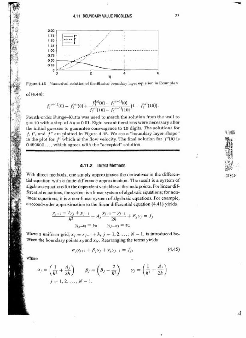
EXAMPLE 4.9 Shooting to Solve the Blasius Boundary Layer

A laminar boundary layer on a flat plate is self-similar and is governed by

f"'+ f f " = 0

where f = f ( q ) and q is the similarity variable. f and its derivatives are pro- portional to certain fluid mechanical quantities: f a i I r , the stream function; f ' = u / U , where u is the local fluid velocity and U is the free stream fluid velocity; and f " a t, the shear stress. Boundary conditions for the equations are derived from the physical boundary conditions on the fluid: "no-slip" at the wall and free stream conditions at large distances from the wall. They are summarized as

. ,

f ' ( o ) = f ( o ) = 0 f l ( o o ) = l .

We wish to solve for f and its derivatives throughout the boundary layer. Since one of the boundary conditions is prescribed at r ] = oo we are required to solve a non-linear boundaly value problem. Solution proceeds by breaking the third-order problem into a coupled set of first-order equations. Taking f i = f ", f 2 = f 1 and f3 = f gives the following set of ordinary differential equations for the solution:

The solution will be advanced from a prescribed condition at the wall, r ] = 0 , to r ] = m. Solutions have been found to converge very quickly for large r ] and marching from r ] = O to r] = 10 has been shown to be sufficient for accurate solution. Two conditions are specified at the wall: f i = O and f3 = O. We must repeatedly solve the whole system and iterate to find the value of fl (O) that gives the required condition, 2 = 1 at r] = m. Two initial guesses were

(f 1 made for f l ( 0 ) : f J o ) ( 0 ) = 1.0 and f l (O) = 0.5. From these two initial guesses two values for f2 at "infinity" were calculated: f P ( 1 0 ) and f P 1 ( 1 0 ) . Starting from these two calculations the secant method may be used to iterate toward an arbitrarily accurate value for f l ( 0 ) based on the following adaptation

4.1 1 BOUNDARY VALUE PROBLEMS

. I

I

4.1 1.2 Direct Methods

With direct methods, one simply approximates the derivatives in the differen-

y(j=O) = YO y(j=N) = 'YL

where a uniform gri4 x j = x j V i + h , j = 1,2, . . . , N - 1, is introduced be-

ajYj+l + Pjy j + yjyj-i = f,, (4.45)

-

j = 1 , 2 , . . . , N - l .


This is a tridiagonal system of linear algebraic equations. The only special treatment comes at the points next to the boundaries j = 1 and j = N - 1. At j = 1, we have

Note that yo, which is known, is moved to the right-hand side. Similarly, yN appears on the right-hand side. Thus, the unknowns y1 , y2, . . . , YN- I are obtained from the solution of

lmplementation of mixed boundary conditions such as

is also straightfonvard. For example, one can simply approximate yf(0) with a finite difference approximation such as

add solve for yo in terms of y l , y2, and g. The result is then substituted in the finite difference equation 4.45 evaluated at j = 1. Because yo now depends on y1 and y2, the matrix elements in %he first row are also modified. Higher order finite difference approximations can also be used. The only difficulty with higher order methods is that near the boundaries they require data from points outside the domain. The standard procedure is to use lower order approximations for points near the boundary. Moreover, higher order finite differences lead to broader banded matrices instead of a tridiagonal matrix. For example, a pen- tadiagonal system is obtained with the standard fourth-order central difference approximation to equation (4.41).

Often the solution of a boundary value problem varies rapidly in a part of the domain, and it has a mild variation elsewhere. In such cases it is wasteful to use a fine grid capable of resolving the rapid variations everywhere in the domain. One should use a non-uniform grid spacing (see Section 2.5). In some problems, such as boundary layers in fluid flow problems, the regions of rapid variation are known a priori, and grid points can be clustered where needed. There are also (adaptive) techniques that estimate the grid requirements as the solution progresses and place additional grid points in the regions of rapid variation.

With non-uniform grids one can either use finite difference formulas written explicitly for non-uniform grids or use a coordinate transformation. Both

EXERCISES 79

techniques were discussed in Section 2.5. Finite difference formulas for first and second derivatives can be substituted, for example, in (4.41), and the resulting system of equations can be solved. ~ l t e r n a t h e l ~ , the differential equation can be transforme4 and the resulting equation can be solved using uniform mesh

EXERCISES

1. Consider the equation

y' + (2 + 0 . 0 1 ~ ~ ) ~ = O

y(0) = 4 o S X ( 10.

(a) Solve this equation using the following numerical schemes: i) Euler, ii) backward Euler, iii) trapezoidal, iv) second-order Runge-Kutta and v) fourth-order Runge-Kutta. Use Ax = 0.1,0.5, 1 .O and compare to the exact solution.

(b) Discuss the stability and accuracy of each scheme. (c) For each scheme, estimate the maximum Ax for stable solution (over the

given domain) and discuss your estimate in terms of results of part (a).

2. A physical phenomenon is governed by the differential equation

d v - = - 0 . 2 ~ - 2 cos(2t)v 2

dt

subject to the initial condition v(0) = 1.

(a) Solve this equation analytically. (b) Write a program to solve the equation for O < t 5 7 using the Euler explicit

scheme with the following time steps: h = 0.2,0.05,0.025,0.006. Plot the four numerical solutions along with the exact solution on one graph. Set the x axis from O to 7 and the y axis from O to 1.4. Discuss your results.

(c) In practica1 problems, the exact solution is not always available. To obtain an accurate solution, we keep reducing the time step (usually by a factor of 2) until two consecutive numerical solutions are nearly the same. Assuming that you do not know the exact solution for the present equation, do you think that the solution corresponding to h = 0.006 is accurate (to plotting accuracy)? Justify your answer. In case you find it not accurate enough, obtain a better one.

r ,>- ?*@*?

3. A physical phenomena is governed by a simple differential equation: f h i L ~ f JsL,3 (j::+$<l$i E ! & .: , v d v : . '1 ., a:<,$, ' " - - r 2 ..

- = -a(t)v + B(t), .:: - >, *j :c.. .32,&. 2% dt bi ',Y;-?< --'A

, , & .$$: ". - pq4 \'i".li.l ~ $ J 2 2

! .-;; >,.*.; 3t 4 ':\..'\. 5 :' :*y . ' r- ,E<* i.'

B(t) = 2(1 + t13e-'. ,, 1,s. ;:%J

a(t) = - 7 -29

(1 + t) \F?&54&23 ,.%F. ,>- Assume an initial value v(0) = 1 .O, and solve the equation for O < t < 15 ~ s i ~ 1 1 0 E e= a the following numerical methods

f


(a) Euler (b) Backward Euler (c) Trapezoidal method (d) Second-order Runge-Kutta (e) Fourth-order Runge-Kutta

Try time steps, h = 0.2, 0.8, 1.1.0n separate plots, compare your results with the exact solution. Discuss the accuracy and stability of each method. For each scheme, estimate the maximum At for stable solution (over the given time domain and over a very long time).

4. Considera simple pendulum consisting of mass m attached to a string of length l. The equation of motion for the mass is

where positive 8 is counterclockwise. For small angles 8, sin 8 6' and the linearized equation of motion is

The acceleration due to gravity is g = 9.81 rn/sec2, and 1 = 0.6 m. Assume that the pendulum starts from rest with B( t = 0) = 10".

(a) Solve the linearized equation for O i: t 5 6 using the following numerical methods:

(i) Euler (ii) Backward Euler

(iii) Second-order Runge-Kutta (iv) Fourth-order Runge-Kutta (v) Trapezoidal method

Try time steps, h = 0.15, 0.5, 1. Discuss your results in terms of what you know about the accuracy and stability of these schemes. For each case, and on separate plots, compare your results with the exact solution.

(b) Suppose mass m is placed in a viscous fluid. The linearized equation of motion now becomes

g 8" + ~ 6 ' ' + -6' = O. 1

Let c = 4 sec-' . Repeat part (a) with methods (i) and (iii) for this problem. Discuss quantitatively and in detail the stability of your computations as compared to part (a).

(c) Solve the non-linear undampedproblem with 0(t = 0) = 60" with a method of your choice, and compare your results with the corresponding exact

linear solution. What steps have you taken to be certain of the accuracy of your results? That is, why should your results be believable? How does the maximum time step for the non-linear problem compare with the prediction of the linear stability analysis?

5 . Consider the pendulum problem of Exercise 4. Recall that the linearized equation of motion is

g 0" = - - O . I

The pendulum starts from rest with O(t = 0) = 10".

(a) Solve the linearized equation for O ( t 5 6 using the following multi-step methods:

(i) Leapfrog (ii) Second-order Adams-Bashforth

Try time steps, h = 0.1, 0.2, 0.5. Discuss youriresults in terms of what you know about the accuracy and stability of these schemes. For each case, and on separate plots, compare your results with the exact solution.

(b) The linearized damped equation of motion is

g 0" + c0' + -e = o. 1

Let c = 4 sec-'. Repeat part (a) for this problem. Discuss quantitatively ., and in detail the stability of your computations as compared to part (a). I

Do your results change significantly using different start-up schemes (e.g., explicit Euler vs. second-order Runge-Kutta)?

6. Double Pendulum (N. Rott) A double pendulum is shown in the figure. One of the pendulums has a space fixed pivot (SFP) and the pivot for the other pendulum (BFP) is attached to the body of the first pendulum. The line connecting the two pivots is of length b and forms an angle Po with the vertical, in equilibrium. The total mass of the two elements is m,, while the BFP pendulum has a mass m, with a distance c between its center of gravity and its pivot. With m, concentrated at BFP, the distance of the center of gravity of the total mass from the SFP is a and the moment of inertia of the two bodies is Ir. The moment of inertia of the BFP

,, pendulum about its pivot is I,. The position angles of the two pendulums with respect to the vertical are a and y , as shown in the figure. The equations of motion are (neglecting friction):

Ir& + am,g sin a + bcrn,[Cp + sp2] = O

I,p + cm,gsin y + bcm,[C& - S&'] = O

C = cos Po cos(a - y) - sin Po sin(a - y )

S = sin Po cos(<r - y ) + cos Po sin(a - y).

NUMERICAL SOLUTION OF ORDINARY DIFFERENTIAL EQULTIONS

Double pendulum: SFP = space-fixed pivot; BFP = body-fixed pivot.

The following nomenclature is introduced:

bcm, w2 -- bcm, h2 cm, - - b = t -- - -b- = 1, g / Il g amt

17.

Here h and w are the frequencies of the uncoupled modes, while ,$ and q are two interaction parameters. Let

Exchange of Energy The pendulum system exhibits an interesting coupling when properly "tuned." In a tuned state the moda1 frequencies are in the ratio 1 :2 (heryo = 2h). Then for particular sets of initial conditions, some special interaction takes place in which the two pendulums draw energy from each other at a periodic rate. In that case, when one pendulum oscillates with maximum amplitude, the other stands almost still and the process reverses itself as the energy passes frorn one pendulum to the other. This phenomenon of energy exchange is periodic if the pendulums are properly tuned. Note that this peculiar motion happens only for well-chosen initial conditions and is usually associated with low energy. Try

Use either your own program, or a canned routine (e.g. Numerical Recipes' odeint or MATLAB's ode4 5) to solve this system. It is important to exper- iment with different time steps or tolerance settings (in the canned routines)

EXERCISES 83

to ensure that the solution obtained is independent of time step (to plotting accuracy).

Plot the angular deflections (a, y) and velocities (&, y). Determine the period of energy exchange. Now, pick another set of initial conditions for which periodic energy exchange occurs and find out if the period of energy exchange remains the same. In either case, you should plot the two angles versus time on the same graph in order to reveal the phenomenon of energy exchange. Note that the equations of motion should be solved for a sufficiently long time to exhibit the global periodic nature of the solution.

Chaotic Solution This system has three degrees of freedom (two angles and two angular velocities inake four, but since the system is conservative, the four states are linked in the total energy conservation equation). It is possible for such a system to experience chaotic behavior. Chaotic or unpredictable behavior is usually associated with sensitivity to the initial data. In other words, chaotic behavior implies that two slightly different initial conditions give rise to solutioiis that differ greatly. In our problem, chaotic solutions are associated with high-energy initial conditions. Try

n a o = - , ko=5rad / s , y,-,=O, yo=O.

2

Simulate the system and plot the two angles versus time. How is the solution different from that ofthe previous section? Now vary the initial angular velocity ciO by 1/2%, i.e. try

n ao=-, cio=5.025rad/s, yo=O, yo=O.

2

Plot the angles versus time for the two cases on the same graph and comment on the effect of the small change in the initial conditions. Sensitivity to initial conditions implies sensitivity to truncation and round-off errors as well. Continue your simulations to a sufficiently large time, say t = 100 sec, and comment on whether your solution is independent of time step (and hence reliable for large times).

7. Consider the following family of implicit methods for the initial value problem, Y' = f (Y)

Y n + i = Yn + h[ef(yn+l) + (1 - @)f(yn)l,

where 8 is a parameter O 5 e 5 1. The value of 8 = 1 yields the backward Euler scheine, and 8 = 112 yields the trapezoidal method. We have pointed Out that not al1 implicit methods are unconditionally stable. For example, this scheme is conditionally stable for O 5 0 < 112. For the case 0 = 114, show that the method is conditionally stable, draw its stability diagram, and compare the diagram with the stability diagram of the explicit Euler scheme. Also, plot the stability diagram of the method for 0 = 314, and discuss possible features ~f the numerical solution when this method is applied to a problem with a

ing exact solution.

8: Non-linear differential equations with several degrees of freedom often exhibit chaotic solutions. Chaos is associated with sensitive dependence to initial conditions; however, numerical solutions are often confined to a so-called strange attractor, which attracts solutions resulting from different initial conditions to its vicinity in the phase space. It is the sensitive dependence on initial conditions that makes many physical systems (such as weather patterns) unpredictable, and it is the attractor that does not allow physical parameters to get out of hand (e.g., very high or low temperatures, etc.) An example of a strange attractor is the Lorenz attractor, which results from the solution of the following equations:

The values of o and b are usually fixed (a = 10 and b = 813 in this problem) leaving r as the control parameter. For low values of r , the stable solutions are stationary. When r exceeds 24.74, the trajectories in xyz space become irregular orbits about two particular points.

(a) Solve these equations using r = 20. Start from point (x, y , z) = (1, 1, l), and plot the solution trajectory for O _( t 5 25 in the xy, xz, and yz planes. Plot also x , y, and z versus t . Comment on your plots in terms of the previous discussion.

(b) Observe the change in the solution by repeating (a) for r = 28. In this case, plot also the trajectory of the solution in the three-dimensional xyz space (let the z axis be in the horizontal plane; you can use the MATLAB command p l o t 3 ( z , y, x ) for this). Compare your plots to (a).

(c) Observe the unpredictability at r = 28 by overplotting two solutions versus . time starting from two initially nearby points: (6,6,6) and (6, 6.01, 6).

9. In this problem we will numerically examine vortex dynamics in two dimensions. We assume that viscosity is negligible, the velocity field is solenoidal (V . u = O), and the vortices may be modeled as potential point vortices. Such a system ofpotential vortices is governed by a simple set of coupled equations:

where (xj, y,) is the position of the j th vortex, o, is the strength and rotational direction of the j th vortex (positive o indicates counter-clockwise rotation),

r i j is the distance between the jth and i th vortices,

(2)

and N is the number of vortices in the system. For example, in the case of N = 2 and wl = w2 = 1, the equations (1 a, b) become

dx 1 - 1 (Y1 - Y2) dy1 1 (XI - x2) - - -- -- - dt 2n r2 d t 2n r2

dx2 - 1 (y2 - ~ i ) dy2 1 (x2 - x1) - - -- - - - d t 2 n r2 d t 2n r 2

= J(xi - x2) + (Y, - ~ 2 ) .

Equations (la) and (lb) rnay be combined into a more compact form if written for a complex independent variable z, with x, = Real[zj] and y j = Imag[zj]:

dz; 1 N -- - dr % z ~ ' (3)

IZi

The * indicates complex conjugate. The system has 2N degrees of freedom (each vortex has two coordinates that

rnay vary independently). There exist four constraints on the motion of the vortices that rnay be derived from the flow physics. They are (at'? very basic level) conservation of x and y linear momentums, conservation of angular momen- tum, and conservation of energy. Conservation of energy is useful as it can give a simple measure of the accuracy of a numerical solution. It rnay be posed as

N N

= const. n n ~ ; ; (4) j i ; ,

For N = 4 there are four unconstrained degrees of freedom or two unconstrained two-dimensional points of the form (p, q). Such a system rnay poten- tially behave chaotically. We will now explore this.

(a) Take N = 4 and numerically solve the evolution of the vortex positions. You rnay solve either Equation (1) or (3). Equation (3) is the more el- egant way of doing it but requires a complex ODE solver to be written (same as a real solver but with complex variables). A high-order explicit scheme is recommended (e.g. fourth-order Runge-Kutta). Numerical Recipes' odeint or MATLAB 'S ode4 5 might be useful. Use as an initial condition (x, y) = (f 1 , f 1); that is, put the vortices on the corners of a Square centered at the origin. Take wj = 1 for each vortex. Solve for a sufficiently long time to see if the vortex motion is "regular." Use the energy constraint equation (4) to check the accuracy of the solution. Plot the time history of the position of a single vortex in the xy plane.

(b) Perturb one of the initial vortex positions. Move the (x, y) = (1, 1) point to (x, y) = (1, 1.01) and repeat part (a).

NUMERICAL SOLUTION OF ORDINARY DIFFERENTIAL EQUATIONS

(c) Consider a case now where the vortices start on the corners of a rectangle with aspect ratio 2: (x, y ) = (f 2, f 1). Repeat (a).

(d) Again perturb one initial position. Move the (x , y) = (2, 1) point to (x , y) =

(2, 1 .O 1 ) and repeat part (a). (e) Chaotic systems usually demonstrate a very high dependence upon initial

conditions. The solutions from similar but distinct initial conditions often diverge exponentially. Place al1 vortices in a line: (x, y)k = (- 1, O), (E, O), (1, O), (2,O) and accurately solve the problem from time O to 4 for E = O and E = 1 Make a semi-log plot of the distance between the vortices starting at (O, 0) and (E, O) versus time for these two runs. Justify the accuracy of the solutions.

10. The following scheme has been proposed for solving y ' = f (y):

Yn+i = ~n + ~ k i + 02k2,

where

with h being the time step.

(a) Determine the coefficients wl , 'a2, Po, and DI that would maximize the order of accuracy of the method. Can you name this method?

(b) Applying this method to y' = ay , what is the maximum step size h for cr pure imaginary?

(c) Applying this method to y ' = ay , what is the maximum step size h for a real negative?

(d) With the constraints derived in part (a) draw the stability diagram in the (hhR, hhI) plane for this method applied to the model problem y ' = Ay.

The following scheme has been proposed for solving y ' = f (y):

where

with h being the time step.

(a) Give a word description of the method in terms used in this chapter. (b) What is the order of accuracy of this method? (c) Applying this method to y ' = ay , what is the maximum step size h for a

pure imaginary and for a negative real?

EXERCISES 87

(d) Draw a stability diagram in the (hhR, hh,) plane for this method applied to the model problem y' = Ay.

Chemical reactions often give rise to stiff systems of coupled rate equations. The time history of a reaction of the following form:

is governed by the following rate equations

where kl , k2, and k3 are reaction rate constants given as

and the Ci are the concentrations of species Ai. Initially, CI (O) = 0.9, Cz(0) = 0.1, and C3(0) = 0. . ! (a) What is the analytical steady state solution? ~ o t e that thdse equations should

conserve mass, that is, Ci + C2 + C3 = 1. (b) Evaluate the eigenvalues of the Jacobian matrix at t = O. 1s the problem

stiff? (c) Solve the given system to a steady state solution ( t = 3000 represents steady

state in this problem) using

(i) Fourth-order Runge-Kutta (use (b) to estimate the maximum time step).

(ii) A stiff solver such as Numerical Recipes' s t i f b s , l s o d e , or MATLAB's o d e 2 3 s.

Make a log-log plot of the concentrations Ci vs: time. Compare the computer time required for these two methods.

(d) Set up the problem with a linearized trapezoidal method. What advantages would such a scheme have over fourth-order RK?

In this problem, we will consider a chemical reaction taking place in our bodies during food digestion. Such chemical reactions are mediated by enzymes, which are biological catalysts. In such a reaction, an enzyme (E) combines with a substrate (S) to form a complex (ES). The ES complex has two possible fates. It can dissociate to E and S or it can proceed to form product P. Such chemical reactions often give rise to stiff systems of coupled rate equations. The time history of this reaction

is governed by the following rate equations

where kl , k2, and k3 are reaction rate constants. The constants for this reaction are

and the Ci are the concentrations. Initially, Cs = 1, CE = 5.0 x lop5, CES = 0.0, Cp = 0.0.

(a) Solve the given system of equations to the steady state using:

(i) Fourth-order Runge-Kutta. (ii) A stiff solver such as Numerical Recipes' S t i f b s , l s o d e , or MAT-

LAB's o d e 2 3 s .

Make a log-log plot of the results. Compare the computer time required for these two methods.

(b) Set up and solve the problem with a linearized trapezoidal method. What advantages would such a scheme have over fourth-order RK?

14. Consider the following three-tube model of a kidney (Ivo Babuska)

where

Solute and water are exchanged through the walls of the tubes. y,, y5, and y3 represent the concentration of the solute in tubes 1, 2, and 3, respectively. y2 and y4 represent the flow rates in tubes 1 and 3. The initial data are

(a) Use a stiff ODE solver (such as Numerical Recipes' S t i f b s , l s o d e , or MATLAB's ode2 3 S) to find the solution for O 5 t 5 1. What kind of gradient inforrnation did you specik if any?

(b) Use an explicit method such as the fourth-order Runge-Kutta method and compare the computational effort to that in part (a).

(c) Set up the problem with a second-order implicit scheme with linearization to avoid iterations at each time step.

(d) Solve your setup ofpart (c). Compare with the other methods. It is advisable to make al1 your plots on a log-linear scale for this problem.

Consider the problem of deflection of a cantilever beam of varying cross section under load P. The differential equation for the deflection y is

where x is the horizontal distance along the beam, E is Young's modulus, and l(x) is the moment of inertia of the cross section. The fixed end of the beam at x = O implies y(0) = yt(0) = O. At the other end, x = 1, the bending and shearing moinents are zero, that is y"(1) = y"'(1) = O. For the beam under consideration the following data are given:

I (x) = 6 x 10-~e-~' ' m4

E = 230 x 1 o9 Pa

Z = 5 m

P = 104x N/m. I

Compute the vertical deflection of the Ileam, y(x). What is the maximum deflection? Where is the maximum curvature in the beam?

It is recommended that you solve this problem using a shooting method. The fourth-order problem should be reduced to a system of four first-order equations in

The general solution can be written as

where + is the particular solution obtained by shooting with homogeneous conditions. The are the solutions of the homogeneous equation with initial conditions ei , where the ei are the Cartesian unit vectors in four dimensions. Show that only three "shots" are necessary to solve the problem and that one only needs to solve a 2 x 2 system of equations to get c3 and cq. In addi- tion, explain why with this procedure only one shot will be necessary for each additionai P that may be used.

The goal of this problem is to compute the self-similar velocity profile of a corn- Pressible viscous flow. The flow is initiated as two adjacent parallel streams that mix as they evolve. After some manipulation and a similarity transformation,

NUMERICAL SOLUTION OF ORDINARY DIFFERENTIAL EQUATIONS

the thin shear layer equations (the boundary layer equations) may be written as the third-order ordinary differential equation:

where f = f (q), q being the similarity variable. The velocity is given by f ' = u / U1, U, being the dimensional velocity of the high-speed fluid. U2 is the dimensional velocity of the low-speed fluid. The boundary conditions are

This problem is more difficult than the flat-plate boundary layer example in the text because the boundary conditions are specified at three different loca- tions. A very accurate solution, however, may be calculated if you shoot in the following manner:

(a) Guess values for f'(0) and f"(0). These, with the given boundary condition f (O) = O, specify three necessary conditions for advancing the solution numerically from q = O. Choose f'(0) = (U1 + U2)/(2Ul), the average of the two streams.

(b) Shoot to q = m . (For the purposes of this problem m is 1 O. This can be shown to be sufficient by asymptotic analysis of the equations.)

(c) Now here's where we get around the fact that we have a three-point boundary value problem. We observe that g(aq) = f (q)/a also satisfies Equation (1). If we choose a = f (1 O), which was obtained in (b), the equ'ation recast in g and the corresponding boundary conditions at zero and m are satisfied.

(d) Now take the initial guesses, divide by a and solve for the lower half of the shear layer in the g variable. You have g(0) = O, gf(0) = f'(O)/a, and g"(0) = f"(O)/a giving the required initial condition for advancing the solution in g from q = O to q = - 10.

(e) Compare the value ofgl(- 1 O) to the boundary condition f'(-m) = U2/ U,. Use this difference in a secant method iteration specifying new values of f"(0) until gl(-10) = U2/ U1 is within some error tolerance.

As iteration proceeds, fixing gl(- 10) to the boundary condition for f'(- 10) in (e) forces a to approach 1 thus making g f , the solution. However, a will not actually reach 1, because we do not allow our f'(0) guess to vary. The solution for g, though accurate, may be further refined using step (f).

(f) Use your final value for gr(0) as the fixed f'(0) value in a new iteration. Repeat until you have converged to a = 1 and evaluate.

Take Ul = 1 .O and U2 = 0.5, solve, and plot f'(q). What was your final value of a ? Use an accurate ODE solver for the shooting. (First reproduce the Blasius boundary layer results given in Example 9 in the text. Once that is setup, then try the shear layer.) How different is the solution after (f) than before with f'(0) = (U1 + U2)/(2Ul)?

17. The diagram shows a body of conical section fabricated from stainless steel immersed in air at a temperature T, = O. It is of circular cross section that varies

with x . The large end is located at x = O and is held at temperature TA = 5. The small end is located at x = L = 2 and is held at TB = 4.

Conservation of energy can be used to develop a heat balance equation at any cross section of the body. When the body is not insulated along its length and the system is at a steady state, its temperature satisfies the following ODE:

where a(x), b(x), and f (x) are functions of the cross-sectional area, heat trans- fer coefficients, and the heat sinks inside the body. In the present example, they are given by

x + 3 a(x) = - - b(x) =

x + 3 and f(x) = 2(x + 1)+3b(x).

x + l l (X + 1)2 '

(a) In this part, we want to solve (1). using the shooting method.

(i) Convert the second-order differential equation (1) to a system of 2 first-order differential equations.

(ii) Use the shooting method to solve the system in (i). Plot the temperature distribution along the body.

(iii) If the body is insulated at the x = L end, the boundary condition becomes dT/dx = O. In this case use the shooting method to find T ( x ) and in particular the temperature at x = L. Plot the temperature distribution along the body.

(b) We now want to solve (1) directly by approximating the derivatives with finite difference approximations. The interval from x = O to x = L is discretized using N points (including the boundary points):

The temperature at point j is denoted by 7''. (i) Discretize the differential equation (1) using the central difference

formulas for the second and first derivatives. The discretized equation is valid for j = 2 , 3 , . . . , N - 1 and therefore yields N - 2 equations for the unknowns TI, T2, . . . , TN.

(ii) Obtain two additional equations from the boundary conditions (TA = 5 and TB = 4) and write the system of equations inmatrix form A T = f . Solve this system with N = 21. Plot the temperature using symbols on the same plot of part (a)(ii).

92 NllMERlCAL SOLUTION OF ORDINARY DIFFERENTIAL EQUATIONS

FURTHER READlNG

Dahlquist, G., and Bjorck, A. Nurnerical Methods. Prentice-Hall, 1974, Chapter 8. Forsythe, G. E., Malcolm, M. A., and Moler, C. B. Computer Methods for Mathe-

matical Computations. Prentice-Hall, 1977, Chapter 6. Gear, C. W. Numerical lnitial Yalue Problems in Ordinary Dzflerential Equations.

Prentice-Hall, 197 1. Press, W. H., Teukolsky, S. A., Vetterling, W. T., and Flannery, B. P. Numerical

Rec@es: The Art of Scientijc Computing, Second Edition. Cambridge University Press, 1992, Chapters 16 and 17.

Documents

Numerical Solution of Ordinary Differential Equationslya.fciencias.unam.mx/gfgf/pa20081/data/material/chap4_engineerin… · Numerical Solution of Ordinary Differential Equations