UPTEC F 17056

Examensarbete 30 hpNovember 2017

Numerical simulations of the power supply to a tidal compensation system for wave energy converters

Camilla Tumlin

Teknisk- naturvetenskaplig fakultet UTH-enheten Besöksadress: Ångströmlaboratoriet Lägerhyddsvägen 1 Hus 4, Plan 0 Postadress: Box 536 751 21 Uppsala Telefon: 018 – 471 30 03 Telefax: 018 – 471 30 00 Hemsida: http://www.teknat.uu.se/student

Abstract

Numerical simulations of the power supply to a tidalcompensation system for wave energy converters

Camilla Tumlin

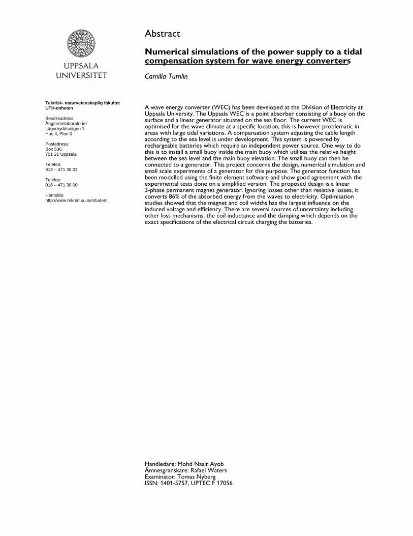
A wave energy converter (WEC) has been developed at the Division of Electricity atUppsala University. The Uppsala WEC is a point absorber consisting of a buoy on thesurface and a linear generator situated on the sea floor. The current WEC isoptimised for the wave climate at a specific location, this is however problematic inareas with large tidal variations. A compensation system adjusting the cable lengthaccording to the sea level is under development. This system is powered byrechargeable batteries which require an independent power source. One way to dothis is to install a small buoy inside the main buoy which utilises the relative heightbetween the sea level and the main buoy elevation. The small buoy can then beconnected to a generator. This project concerns the design, numerical simulation andsmall scale experiments of a generator for this purpose. The generator function hasbeen modelled using the finite element software and show good agreement with theexperimental tests done on a simplified version. The proposed design is a linear3-phase permanent magnet generator. Ignoring losses other than resistive losses, itconverts 86% of the absorbed energy from the waves to electricity. Optimisationstudies showed that the magnet and coil widths has the largest influence on theinduced voltage and efficiency. There are several sources of uncertainty includingother loss mechanisms, the coil inductance and the damping which depends on theexact specifications of the electrical circuit charging the batteries.

ISSN: 1401-5757, UPTEC F 17056Examinator: Tomas NybergÄmnesgranskare: Rafael WatersHandledare: Mohd Nasir Ayob

Contents

Popularvetenskaplig sammanfattning 1

1 Introduction 31.1 Wave power . . . . . . . . . . . . . . . . . . . . . . . . . . . . 31.2 Uppsala University WEC . . . . . . . . . . . . . . . . . . . . . 51.3 Problem statement . . . . . . . . . . . . . . . . . . . . . . . . 9

2 Theory 112.1 Water wave theory . . . . . . . . . . . . . . . . . . . . . . . . 112.2 WEC model for a point absorber . . . . . . . . . . . . . . . . 122.3 Electromagnetism . . . . . . . . . . . . . . . . . . . . . . . . . 142.4 Permanent magnet generators . . . . . . . . . . . . . . . . . . 152.5 Electrical damping circuits . . . . . . . . . . . . . . . . . . . . 172.6 Finite element method . . . . . . . . . . . . . . . . . . . . . . 20

3 Numerical modelling 223.1 COMSOL Multiphysics . . . . . . . . . . . . . . . . . . . . . . 223.2 Simulink: Electrical circuit model . . . . . . . . . . . . . . . . 26

4 Prototype experiment 274.1 Experimental set up . . . . . . . . . . . . . . . . . . . . . . . 274.2 Numerical model . . . . . . . . . . . . . . . . . . . . . . . . . 284.3 Experimental results . . . . . . . . . . . . . . . . . . . . . . . 294.4 Stator iron . . . . . . . . . . . . . . . . . . . . . . . . . . . . . 33

5 Full size generator model 355.1 Magnetic fields and induced voltage . . . . . . . . . . . . . . . 355.2 Power, damping and efficiency . . . . . . . . . . . . . . . . . . 405.3 Parameter dependence . . . . . . . . . . . . . . . . . . . . . . 42

6 Discussion and conclusions 486.1 Future research . . . . . . . . . . . . . . . . . . . . . . . . . . 50

Acknowledgements 51

References 52

Popularvetenskaplig sammanfattning

Utvecklandet av alternativa fornyelsebara energikallor ar en nodvandighetfor att stalla om vart nuvarande fossilbaserade energisystem. En till storadelar outnyttjad resurs finns i haven dar vattnets naturliga rorelser, sa somvagor och strommar, kan anvandas for att utvinna energi. Vid avdelnin-gen for elektricitetslara pa Uppsala Universitet har en vagenergiomvandlareutvecklats som utnyttjar havsvagors vertikal rorelser genom att lata en bojvid vattenytan driva en linjargenerator som star pa botten. Generatorn om-vandlar den mekaniska rorelsen fran bojen till elektrisk energi. Generatornbestar av en translator med permamentmagneter som ror sig upp och nerinuti en stator med spolar. Det varierande magnetfaltet fran translatornsrorelse inducerar strom i dessa enligt Faradays induktionslag.

Vagenergiomvandlaren dimensioneras for ett specifikt vagklimat, detta ardock problematiskt pa platser dar havsnivan varierar flera meter pa grund avtidvattnet. For att generatorn ska prestera optimalt behover translatorn varacentrerad vertikalt i statorn for att absorbera all energi fran vagorna. Denkabel som kopplar samman bojen och translatorn ar i nulaget fix, sa storatidvattenvariationer innebar betydande forluster i form av minskad energiab-sorption. Ett kompensationssystem ar darfor under utveckling vid avdelnin-gen for elektricitetslara. En vinsch vevar upp eller ner en kedja och kanpa sa satt justera langden pa forbindelsen mellan boj och translator utefterhavsnivan. For att driva vinschen anvands en motor och laddningsbara bat-terier. For att ladda batterierna behovs ett separat energiutvinningssystem.Solceller kan tacka delar av behovet, men ett komplementterande systembehovs. Ett forslag ar att konstruera en mindre version av ett vagkraftverkinuti vagkraftverkets huvudboj. Skillnaden mellan vattennivan och huvud-bojens position i vattnet kan utnyttjas genom att ha en cylindrisk halighetoch en mindre boj pa undersidan av den storre bojen. Den mindre bojen rorsig darfor aven den upp och ner och kan pa sa satt kopplas till en generatorfor att utvinna energi.

Detta examensarbete undersoker en mojlig konstruktion av generatorgivet ett visst vagklimat och begransningar i storlek och vikt for generatorn.Projektet bestar i huvudsak av numeriska berakningar for dimensioneringenav en linjar generator. Dessa har gjorts i COMSOL Multiphysics, ett simuler-ingsprogram baserat pa finita elementmetoden. Experiment har aven utforts

1

med en mindre, enklare version av generatorn for att delvis kunna verifieraden numeriska modellen. De experimentella testerna stamde over lag valoverens med modellen. For att fa en indikation pa effekten av jarnet i sta-torn sa utfordes aven ett test med en smal bit jarn utanpa spolen. Det hadeen markbar effekt pa translatorns rorelse, vilken tenderade att da stanna avinuti spolen.

Modellen for den fullskaliga generatorn har anvants for att simulera dessfunktion och identifiera vilka designparametrar som paverkar mest. Denforeslagna generatorn ar linjar med tre faser, bestaende av en translator medpermanentmagneter fastsatt pa ett metallror och en stator med sex spo-lar omgivna av jarn. Spolarna kopplas till en elektrisk krets som likriktarstrommen och driver en last, har ett motstand. Den foreslagna designenkonverterar 86% av den inkommande energin i vagorna till elektrisk en-ergi. Detta tar dock enbart hansyn till kopparforluster i spolarna. Storaosakerheter i spolarnas induktans samt andra forluster i form av friktion ochvirvelstrommar i jarnet i statorn betyder att detta sannolikt ar en ovre grans.

Ett antal olika parametrar varierades for att undersoka deras inverkanpa effektiviteten. Magneternas och spolarnas bredd hade storst paverkan paden inducerade spanningen. Storlek och antal kablar som anvands i spolarnahar ocksa en inverkan, fler antal varv inducerar mer spanning samtidigt somdet okar resistansen och induktansen i spolarna.

Denna modell baseras pa ett antal forenklade antaganden, ignorerar flerakallor till forluster och har undersokt langt ifran alla fria variabler. En bety-dande begransning i modellen ar att den antar att den mindre bojen kommeratt rora sig pa ett visst satt (ha en fordefinierad dampning) och sedan an-passas lasten sa att det overensstammer. Modellen kan anvandas som ettdimensioneringsverktyg vid sidan av konstruktionen snarare an att ge enfardig design. For den faktiska konstruktionen behover sannolikt ytterligareett antal restriktioner tas i beaktan.

2

1 Introduction

1.1 Wave power

The wave power group at the Division of Electricity at Uppsala Universitystudies the possibilities of harnessing the energy contained in ocean wavesand converting it to electrical energy. Wave energy is an active area of re-search and remains a largely untapped renewable energy resource. Albeit nota new concept, it has not yet seen the rapid development and deploymentof some other renewable energy resources in the recent years, namely windand solar power. The theoretical energy contained in ocean waves globallyreaches the scale of PWh (1012 kWh) per year, but is greatly reduced whenconsidering the technical and economical limitations [1]. The energy flux forocean waves is predominantly given as average power per meter of wave crest.The wave resource at the coast naturally varies around the world but canreach up to 100 kW/m, while the Swedish west coast has an average energyflux of just over 5 kW/m [2].

One of the main disadvantages of wave energy is the random motion ofthe waves, requiring energy conversion and storage systems to smooth thepower output [3]. In addition, the harsh sea environment puts high demandson the structural mechanics and materials of a wave energy converter. Thusit is also challenging to make power from ocean waves economically feasible[1]. Wave power does however have the advantage of higher energy densitycompared to wind due to higher density of water, the power density is 2-3kW/m2, which is around 5 times the energy density of wind power [4]. Inaddition, it has a higher utility grade (up to 90%) compared to wind and so-lar (20-30%) [5]. The wave power resource is also easier to predict comparedto wind and has little environmental impact. Furthermore, it can be placednear demand since over a third of the world population lives within 90 kmof the coast [3].

A large number of wave energy converter (WEC) prototypes have beensuggested with different working principles and uses. The devices can be cat-egorised in several different ways, for example by location such as onshore,near shore or off shore. Alternatively, by working principle such as oscillat-ing bodies, pressure differential or overtopping devices. The most commondevice is the point absorber, floating devices which are small compared to

3

the wave length. These use the heaving or pitching motion of the waves toharness the energy. This is the type of device studied at Uppsala University(see more in the next section). Reviews of the different technologies can befound in for example Refs. [3] and [5].

Converting the energy absorbed from the waves is done by a power take-offsystem (PTO). There are several different ways to do this: pneumatically,hydraulically or mechanically, and in one or several conversion stages [3].Pneumatic and hydraulic systems use a pressurised medium to convert thelow frequency wave motion to high-speed motion driving a conventional ro-tational generator. This does however incur conversion losses and increasesthe complexity [6]. Mechanical PTO systems can be either direct-driven orhave one or several conversion stages. A comparison of different direct-driveand linear-to-rotary PTO systems is found in Ref.[7]. In this study, mod-elling and lab tests showed that linear generators had highest potential interms of energy production and cost of energy. However, material and com-ponent cost and availability are also important factors, e.g. the ability topurchase standard rotary permanent magnet generator might be more im-portant. An alternative direct-driven energy capture system using so calleddielectric elastomers is studied and tested in Ref.[8]. This systems works asa reverse ”artificial muscle”, where mechanical stretching of an elastomer-electrode sandwich can amplify an applied voltage (working as a capacitorwith varying capacitance).

Wave energy devices exists for both electricity supply for the grid andfor stand-alone applications. Small scale autonomous WECs have differentrequirements compared to high-power, large-scale devices. These are oftenstudied in the context of ocean monitoring, in particular remote sensor buoyscarrying various measuring equipment. These typically rely on solar panelsand battery systems and/or are designed to sink when the batteries are unus-able [9–11]. There are different types of autonomous WECs, for example onesconverting energy using an oscillating water column (OWC) [10] or a pointabsorber. They can also be direct driven [12] or have a system convertinglinear to rotary motion [9, 11, 13].

4

1.2 Uppsala University WEC

The WEC developed at Uppsala University (and Seabased Industry AB) isa point absorber with a floating buoy moving with the heave of the waves.It is connected to a linear generator stationary on the sea floor, see Figure1. A cable connects the buoy to a translator with permanent magnets on itand a voltage is induced in the windings of the stator when the buoy movesup and down. The WEC has been tested at a research site outside of Lysekilsince 2004 and a large number of doctoral theses has contributed to the de-velopment, from mechanical design to grid connection [14].

Figure 1: Sketch of the Uppsala University WEC [15].

One of the latest developments for the Uppsala WEC is studying thepower absorption losses due to tidal effects, this is evaluated in Ref.[16]. Thelength of the cable connecting the translator to the buoy is determined by the

5

deployment site. However, if the site is subject to large variations in sea leveldue to the tide, the WEC will perform sub-optimally for large parts of theday when the cable is either slack or the buoy submerged. Areas with lossesover 50% (compared to WEC without tidal compensation system) includethe west coast of England and Wales, the south coast of Argentina and thenorth-west coast of Australia [16].

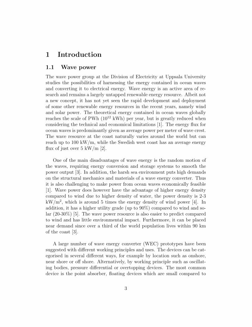
A tidal compensation system for tidal ranges up to 8 m is under develop-ment in the wave power group where a 1.5kW DC motor powers a winch usedto retract or release a cable depending on the sea level [17]. The motor runsoff rechargeable 12V lead acid batteries and the system requires an averageof 38 W for a tidal range of 8 m. An initial study by the supervisor inves-tigates solar panels, an oscillating water column (OWC) WEC and a smallheaving point absorber WEC. This study revealed that an OWC would notbe able to provide sufficient power, while the small point absorber togetherwith solar panels could. The idea of the small point absorber WEC is thatit utilises the relative difference between the wave height and the position ofthe main buoy, see Figure 2. The incoming wave and resulting motion of themain and small buoy is calculated numerically in MATLAB, the result canbe seen Figure 3. The script was provided by the supervisor and is describedin more detail in Section 2. The motion is calculated for specific wave climateand the power absorbed depends on the damping of the system. The mostpower absorbed by the small buoy was found to occur for a generator damp-ing coefficient of 400 Ns/m for the most common wave, with little variationin power output above that. Figure 4 shows the average power output fordifferent damping coefficients.

6

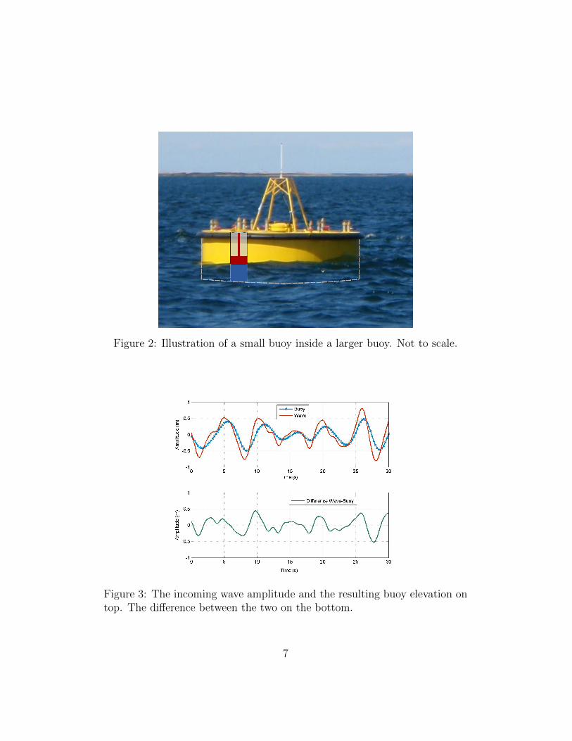
Figure 2: Illustration of a small buoy inside a larger buoy. Not to scale.

Figure 3: The incoming wave amplitude and the resulting buoy elevation ontop. The difference between the two on the bottom.

7

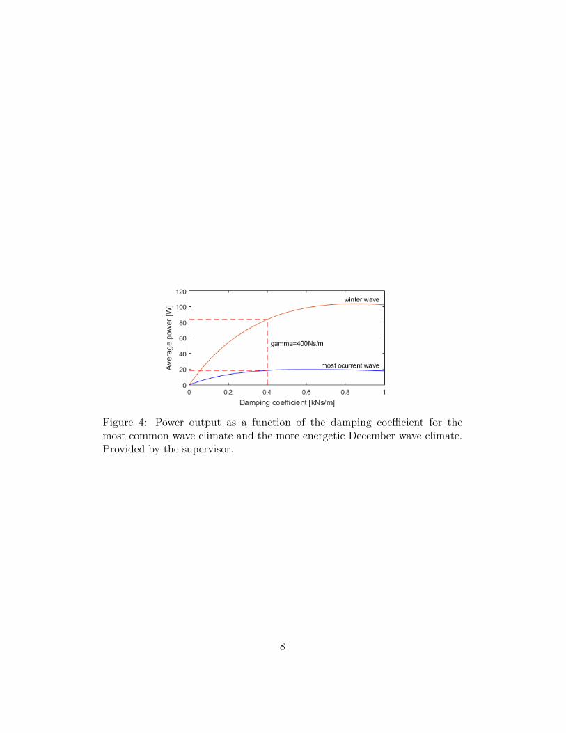
Figure 4: Power output as a function of the damping coefficient for themost common wave climate and the more energetic December wave climate.Provided by the supervisor.

8

1.3 Problem statement

This project concerns the energy supply for the rechareable batteries for thetidal compensation system. It focuses on designing a generator for the smallbuoy set-up that fits the following specifications: a maximum diameter of 35cm, total mass of 20 kg and stroke length of 1 m. In addition, a minimumdamping coefficient of 400 Ns/m is desired. In Ref.[11], a similar scale pointabsorber WEC in similar wave conditions was demonstrated to generate 20-50 W of power. The authors chose a rotary generator over the direct drivelinear generator for efficiency reasons across different sea states. It does nev-ertheless show that it is feasible to obtain the desired power output using adevice this size.

The design process consists of numerically simulating a linear permanentmagnet generator. The numerical model is described in detail in Section 3.The simulations are done using mainly COMSOL Multiphysics, a commer-cial software tool used for simulating different physical problems with thefinite element method. COMSOL Multiphysics enables simulation of differ-ent branches of physics within the same model, for example magnetic fields,moving or deformed geometries and structural mechanics. The electrical cir-cuit in this project has been modelled using Simulink. Simulink is a blockdiagram environment integrated in MATLAB used for simulating dynamicsystems.

1.3.1 Limitations

This project serves as a starting point for the design of the generator. Theviability of other possible types of generators (e.g rotary) and PTO systemshas not been explored. In addition, even when limiting the study to a linearpermanent magnet generator the parameter space to explore is very large.Some are chosen arbitrarily and studying the effects of all of these is outsidethe scope of this project. A number of simplifications have naturally beenmade, including ignoring losses other than resistive losses in the copper wind-ings and assuming simple air-cored coils with constant inductance. The costand availability of components and manufacturing have not been consideredin this project. The design of the support structure and buoy-generator con-nection has also not been included.

9

A major limitation in how the modelling is done is that a specific dampingcoefficient is assumed for the input motion of the translator. This leads tosomewhat circuitous calculations. First a damping coefficient is specifiedwhich leads to a set movement of the small buoy, from this the power outputand damping is calculated. The load resistance is in turn adjusted until thedamping matches the specified input damping coefficient.

1.3.2 Outline of report

Following this introduction, some fundamental theory is covered in Section2. The basic components of the numerical model is the explained in Section3. A prototype of the generator was constructed and some experiments wereperformed to validate the numerical model. Section 4 describes the experi-ment, the adapted numerical model and the results. Following this is a moredetailed description of the full-scale model for the proposed design in Section5. Here the resulting magnetic fields, induced voltage, power output and effi-ciency for the model is presented. The section also includes the results fromparameter variability studies. Finally, a discussion and concluding remarksare found in Section 6.

10

2 Theory

2.1 Water wave theory

The behaviour of ocean waves are commonly described by linear water wavetheory. Conservation of mass for a fluid with density ρ and moving withvelocity v gives the so called continuity equation:

∂ρ

∂t+∇ · ρv = 0. (1)

For point absorber WECs we are interested in surface gravity waves, i.e.waves with amplitudes small compared to the depth and where gravity is therestoring force. A disturbance generating a surface deformation of a fluid in auniform gravitational field will result in a propagating wave. The motion doesnot propagate far below the surface and thus one can linearize the problemassuming that the wave amplitude resulting from the displacement is smallcompared to the wave length [18].

Assuming ideal (ignoring viscosity) and irrotational flow of an incom-pressible fluid (ρ is constant), the continuity equation reduces to

∇ · v = 0. (2)

Defining a velocity potential v = ∇φ we can write Eq.(2) as

∇2φ = 0. (3)

The vertical displacement from a mean sea level of a small amplitudewave propagating in two dimensions can be described by the free surfaceη(x, t), see Figure 5. Applying appropriate dynamic and kinematic boundaryconditions on the surface and the bottom relating η and φ, Eq.(3) can besolved for η(x, t). Details can be found in for example Ref.[18], the resultcan be written

η(x, t) =H

2tan(kh) cos(kx− ωt). (4)

Here H is the wave height, h(x) is the depth, k the wave number and ω theangular frequency. For tidal variations one can superimpose a low frequencywave with a period matching that of the tidal cycle [1].

11

x

z z = η(x, t)

h(x)

H

Figure 5: Surface gravity waves propagating in one dimension.

2.2 WEC model for a point absorber

A point absorber can convert energy from the wave using the heaving andpitching motion, however, a point absorber like the Uppsala WEC where thebuoy is connected to a linear generator on the bottom only absorbs powerthrough the heave motion. The power absorbed depends both on the charac-teristics of the point absorber and the PTO system providing the damping [6].

The vertical acceleration z of the point absorber (buoy and translatorwith mass m) assuming a stiff cable connection is given by Newton’s secondlaw as:

mz = Fg + Fgen + Fbuoy (5)

where Fg is the force due to gravity, Fgen the damping force from the gener-ator and Fbuoy is the hydrodynamic force on the buoy [19]. If the generatorhas springs or end stops at the bottom or top, these would also be presentin the above expression. The damping force is given by

Fgen = −γz, (6)

where the damping coefficient γ is in general dependent on both the velocityand the position of the translator [20].

The hydrodynamic force on the buoy is divided into three contributions,excitation (Fe), radiation (Fr) and hydrostatic (Fh) [19]:

Fbuoy = Fe + Fr + Fh. (7)

12

For a cylindrical buoy with radius a we have

Fh = −ρgπa2z (8)

and the Fourier transforms of Fe and Fr as

Fe(ω) = feη Fr(ω) = −(R + iωma)ˆz. (9)

The parameters R, ma and fe are functions of ω and are obtained from thesimulation software WAMIT. The incoming wave data is generated randomlygiven input location specific input parameters: the energy period Te and thesignificant wave height Hs [19].

Taking the Fourier transform of Eq.(5) and substituting in the expressionsfor the forces we can write

z = H(ω)η(ω) (10)

where H is then identified as the transfer function from the amplitude ofthe incoming wave, the free surface η, to the buoy elevation z. In the timedomain the buoy elevation z(t) is then the convolution between the transferfunction H(t) and the incoming wave function η(t)

z(t) = H(t) ∗ η(t). (11)

Thus, the motion of the buoy can be determined given the incoming wavefunction and the transfer function which depends on the WEC specificationsand the damping of the PTO system.

Having solved for the buoy elevation, the power extracted during the timefrom 0 to t seconds can be found using [19]

P (t) =1

t

∫ t

0

γz2dt. (12)

13

2.3 Electromagnetism

The fundamental equations governing electromagnetic phenomena are Maxwell’sequations. These equations reflect the fact that charge densities (ρ) and cur-rents (J) are the sources for the electromagnetic fields E and B [21]. Indifferential form they are given as follows

∇ · E =ρ

ε0∇ ·B = 0

∇× E = −∂B

∂t

∇×B = µ0J + ε0∂E

∂t

(13)

(14)

(15)

(16)

The reciprocal relationship, i.e. the effect of the fields on a charge q movingwith velocity v is given by the force law

F = q (E + v×B) . (17)

The underlying principle behind electric machines in general, and per-manent magnet generators in particular Faraday’s law, Eq.(15). It statesthat a time-varying magnetic field (RHS of Eq.(15)) induces an electric fieldaccording (LHS of Eq.(15)). The total magnetic flux over an area S is

Φ(t) =

∫S

B(t)dA. (18)

Using Stokes theorem to rewrite Eq.(15) and Eq.(18) we find that in a closedconductor, a change in the flux Φ of B through the enclosed area of theconductor induces a voltage Vind:

Vind = −dΦ

dt. (19)

The induced current in the loop will flow in the direction so as to oppose thechange in the magnetic field, this is known as Lenz’s law [21].

14

In fact, any material with free conduction electrons subject to a changingmagnetic field will have currents induced within the material, so called eddycurrents. These currents will as above flow so as to oppose the change andthus giving rise to an opposing force. This phenomenon is applied in forexample magnetic brakes and metal detectors [22]. However, for generatorsthis is a source of unwanted damping and power loss. The effects of eddycurrents are difficult to calculate but can be reduced by for example laminat-ing a material to reduce the available path length of the circulating currents[21], see more in the section on permanent magnets generators below.

2.3.1 Magnetic materials

A ferromagnetic material is a material that retains its magnetisation withoutan external magnetic field. Magnetisation of a ferromagnetic material is dueto the alignment of dipoles associated with the quantum spins of unpairedelectrons. In a ferromagnet these dipoles line up with their neighbours andform tiny domains where they all have the same direction. The domains arerandomly distributed so that no macroscopic magnetisation occurs. However,if an external magnetic field is applied, the domains boundaries move andif the external field is strong enough the material becomes saturated, withonly one domain remaining, this is a permanent magnet. It is not enoughto reduce the magnetic field to zero to demagnetise the material, it requiresan external magnetic field to be applied in the opposite direction [21]. Thisprocess of magnetisation and demagnetisation traces out a so called hysteresisloop, seen in Figure 6. Changing the direction of the magnetisation requiresenergy and a ferromagnetic material can be soft or hard depending if thisprocess requires a small or large amount of energy respectively.

2.4 Permanent magnet generators

Permanent magnet generators can be either rotary or linear, consisting ofa stator and either a rotor (rotary generators) or translator (linear genera-tors), coil windings and an arrangement of permanent magnets. The relativemotion of the permanent magnets with respect to the coils will produce achanging magnetic field, inducing a current in the coil windings according toEq.(19).

Outside of the coils there are commonly a soft iron backing and teeth

15

H

B

Saturation

Saturation

Figure 6: Hysteresis loop for a ferromagnetic material. The dashed line showsthe initial magnetisation from a non-magnetised material.

in between the coils to guild the magnetic flux. However, the teeth cancause undesired attraction and cogging forces (i.e. the magnets clinging tothe stator teeth), consequently putting high demands on support structures[4, 23]. Calculating the cogging force and normal force in the air gap fordesigning the support structure can be done analytically or using FEM, seefor example Ref.[24]. For magnets with remanent flux density Br and relativepermeability µr the air gap flux density Ba can be calculated as

Ba =Brlpmµr

lag + (lfeAag/µfeAfe) + (lpmAag/µrApm). (20)

Here l and A are the path length and cross sectional area of the flux throughthe air gap, permanent magnet and iron (subscripts ag, pm and fe respec-tively).

There are different types of losses present in a generator: losses from fric-tion between the mechanical parts, copper losses in the coil windings, hys-teresis losses (changing magnetisation of the materials as discussed above)and eddy current losses [20, 25]. The copper losses are dominant for lowspeed, low frequency applications [20]. While it is possible to reduce lossesin coils by switching inactive coils off [26], it does require many power elec-tronic components. The power loss in the coils is given by the current and

16

the resistance of the windings according to Ohm’s law.

The hysteresis losses depend on the material, magnetic flux density andthe frequency, and the per volume power loss can be estimated as [25]

physteresis = khB2maxω (21)

where kh is a material parameter, Bmax is the maximum magnetic flux den-sity and ω the angular frequency. The losses from one period is given by thearea of the hysteresis loop for the material as in Figure 6.

Significant losses due to eddy currents in a stator steel backing can begreatly reduced when using laminated steel [25]. The per volume eddy cur-rent losses in a laminated material with conductivity σ can be estimatedusing the formula [27]

peddy =σω2d2lamB

2max

6(22)

where dlam is the thickness of the laminates (valid assuming the laminatesare thinner than half the skin depth of the material).

2.5 Electrical damping circuits

The damping from the PTO depends on both the generator properties andload control strategy. The control can be active (using wave prediction) orpassive (optimised for a given sea state) and can be done in numerous differ-ent ways. The review in Ref.[6] concluded that the optimal damping circuitwill depend on the specific WEC design as well as the sea state. Experimen-tal tests for different loading circuits has been done in Ref.[14].

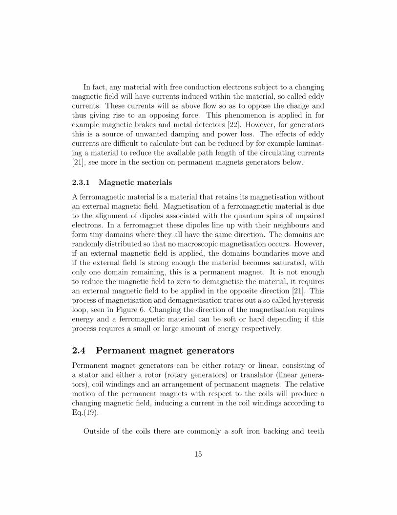
A direct drive point absorber WEC can be represented by an equivalentelectrical circuit model. In Figure 7 one can identify the following: Waveexcitation is represented by voltage V , mass of the device represented by in-ductance L, mechanical damping by resistance R and if a spring is attachedthen the reciprocal of the spring stiffness is represented by capacitance C.The impedance ZPTO represents the load from the PTO system [28].

The load resistance determines the damping from the electrical systemand this needs to be tuned right: too high means less damping (thus less

17

power) and too low results in high dissipation in generator windings [6]. Theelectrical damping force Fem (in the opposite direction to the velocity) canbe written

Fem =Ptot

z(23)

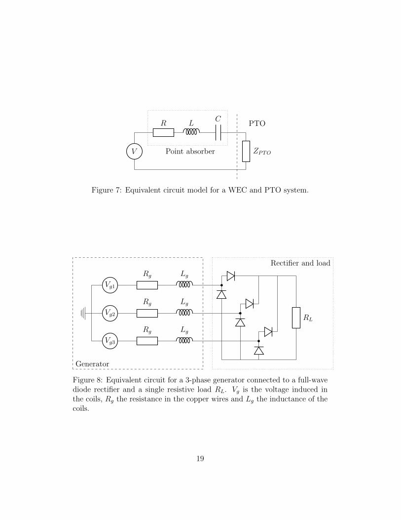
where Ptot is the total power absorbed in the generator. The equivalent circuitof a 3-phase generator and a diode bridge rectifier connected to a resistiveload is shown in Figure 8. For a 3-phase circuit, the damping coefficient isfound to be [29]

γ = 3

[1

Rg

(Vgz

)2

+1

Rload

(Vloadz

)2]. (24)

However, γ is commonly assumed to be independent of z for highly resistiveloads (RL >> Rg) [29].

The internal resistance of the generator mainly consists of the resistivityof the conductors in the coils, thus dependent on the properties of the coilwindings. The generator inductance will vary with the magnetic flux andthe current in the circuit [14]. Efforts have been made to try and estimatethe inductance of the coils in a linear permanent magnet generator [30] andgeneral stacked multi-layer coils [31]. As a first order approximation, theinductance of the coils can be estimated using

L = µ0µrN2

turnsAcoil

l(25)

where Nturns is the number of turns, Acoil is the coil area and l is the lengthof the coil [22]. This assumes a fixed core with a material having relativepermeability of µr inside the coil.

18

V

R

Point absorber

LC

ZPTO

PTO

Figure 7: Equivalent circuit model for a WEC and PTO system.

Vg1

Vg2

Vg3

Rg

Rg

Rg

Lg

Lg

Lg

RL

Generator

Rectifier and load

Figure 8: Equivalent circuit for a 3-phase generator connected to a full-wavediode rectifier and a single resistive load RL. Vg is the voltage induced inthe coils, Rg the resistance in the copper wires and Lg the inductance of thecoils.

19

2.6 Finite element method

Many physics phenomena are described by partial differential equations thatare often inherently difficult or impossible to solve analytically except forspecial cases. A well-used numerical method is the finite element method(FEM). This method was first applied to structural mechanics problems buthas since been expanded to any area where solving partial differential equa-tions is involved. FEM calculations can be very computationally expensive,especially for complex geometries, but rapidly increasing computing powerbecoming available in the last few decades has enabled a widespread uptakeand increasing number of applications [32].

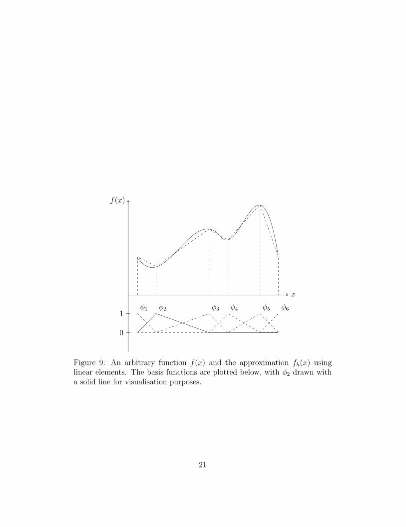
The basic idea behind finite element methods is to divide a geometryinto a discrete number of subdomains (finite elements) and use numericalmethods to find an approximate solution to the required equations [32]. Anunknown continuous function f(x) can be written as a linear combination ofa set of basis functions φ and approximated by the finite sum

f(x) ≈ fh(x) =∑i

ciφi (26)

where ci are unknown coefficients to be solved for. An example of an approxi-mated function f(x) using five elements is shown in Figure 9. Using the basisfunctions, a method can be formulated to obtain a system of linear equationswhich, with appropriate boundary conditions, can be solved numerically.

In order to ascertain that the approximate finite element solution is goodenough a convergence study is required. The mesh is made successively fineruntil the solution is considered converged, with the requirement for conver-gence is dependent on the problem at hand. The element order (degree ofthe basis functions) can also be increased to obtain a more accurate solution.

20

x

f(x)

φ1 φ3 φ5φ4 φ6φ2

0

1

Figure 9: An arbitrary function f(x) and the approximation fh(x) usinglinear elements. The basis functions are plotted below, with φ2 drawn witha solid line for visualisation purposes.

21

3 Numerical modelling

The main focus of this project is the numerical modelling and will be de-scribed in general terms below. Section 4 will then describe the specificmodel used for the experimental prototype tests. Following that, Section 5will discuss the simulation results for the full size generator.

The generator design is tubular so that a 2D axisymmetric (rotationalsymmetry) set-up can be used for the simulations. This reduces the com-plexity and computing time significantly compared to a full 3D geometry.The tubular design has been studied for example in Refs. [4, 23, 33, 34]and has some advantages over designs with flat sides [35], for example a bet-ter force to weight ratio [36]. However, for this project the main reason iscomputational considerations.

3.1 COMSOL Multiphysics

The model is built in COMSOL Multiphysics by drawing the geometry, con-structing the mesh and adding physical properties on a 2D cross section inthe rz-plane (the z-axis is in the axial direction of the generator). The gen-erator consists of a core tube with magnets mounted on it, coil windings anda soft iron backing. The magnets and core tube make up the translator. Thedifferent parts of the model are shown in Figure 10.

The magnets in the model are assumed to be solid rings due to the cylin-drical symmetry. However, they will in reality be individual rectangularmagnets mounted on the outside of the core tube, see Figure 10. A factorRfac adjusting the remanent flux density of the magnets is added to accountfor this difference. This factor depends on the number of magnets used, theirsize and the size of the inner tube, see more on this in Section 4 where theexperimental test is described.

The stator consists of six coil windings, three phases connected in series.The coils are assumed to consist of insulated stranded cables with a specifieddiameter. The number of coil turns depends on the coil area and the crosssection area of the cables. A filling factor of 0.9 is added since it is notpossible to fill the entire space. Between the coils there are iron teeth andan iron backing is wrapped around the outside of the coils.

22

Figure 10: 2D axisymmetric and 3D view of the geometry of the generatorshowing the different parts

3.1.1 Materials

The properties of the magnets are given by data sheets from the supplier.The stator iron is assumed to be soft iron (to reduce hysteresis losses) usingthe built-in material properties COMSOL provides. The baseline simulationshave been done assuming zero electrical conductivity in the soft iron.

3.1.2 Physics modelling

In COMSOL, modules are added for modelling different branches of physics.To model the magnetic fields, current densities and coils, the Magnetic Fieldsmodule is used. Here the magnetic properties of the materials are specified.The constitutive relation for the soft iron is given by the BH-curve and forthe magnets by the remanent flux density. The coil properties are also de-fined here, for example the number of turns and the coil wire cross sectionalarea, as well as appropriate boundary conditions.

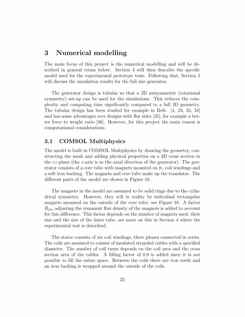
Since the magnets are moving, the Moving Mesh module is added wherethe position of the magnets are specified. The position is obtained from theprovided MATLAB model, described in Section 2. The wave motion over a10 second interval for three different damping coefficients is shown in Figure11.

23

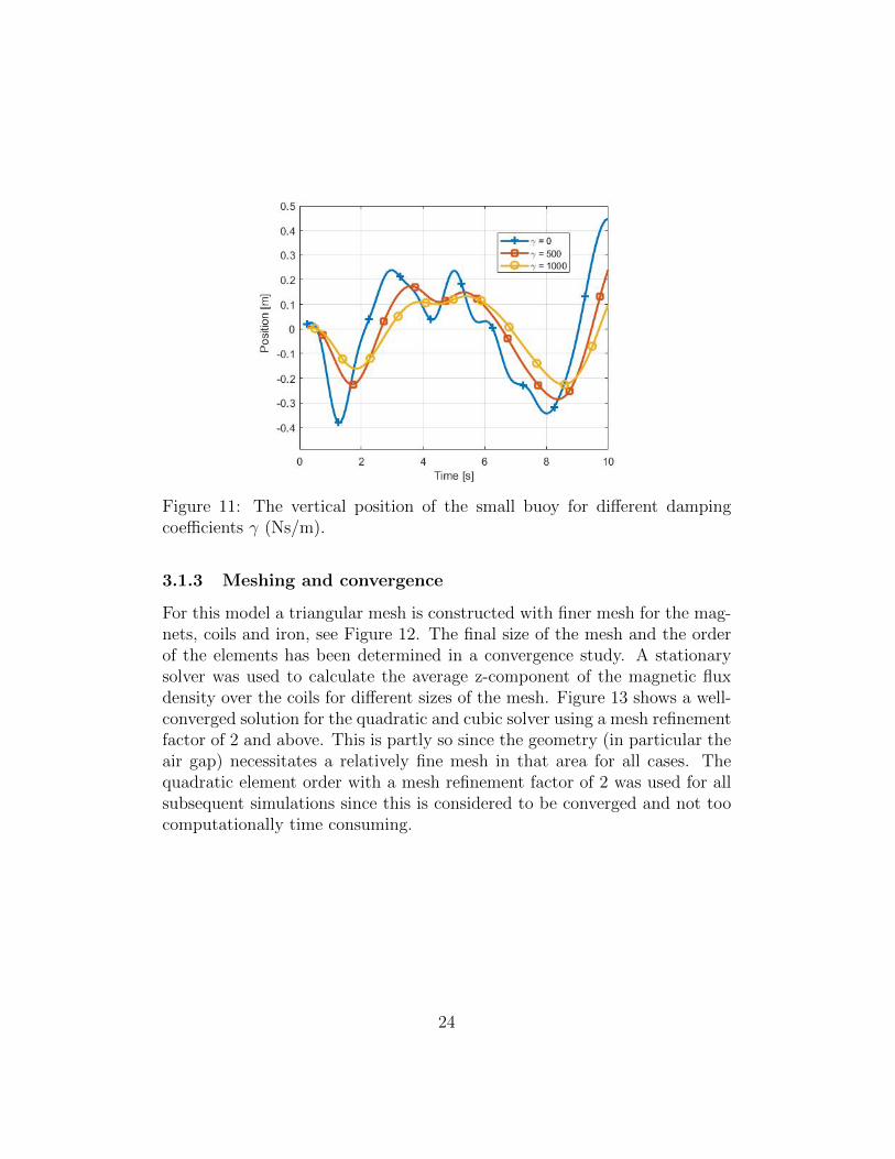
Figure 11: The vertical position of the small buoy for different dampingcoefficients γ (Ns/m).

3.1.3 Meshing and convergence

For this model a triangular mesh is constructed with finer mesh for the mag-nets, coils and iron, see Figure 12. The final size of the mesh and the orderof the elements has been determined in a convergence study. A stationarysolver was used to calculate the average z-component of the magnetic fluxdensity over the coils for different sizes of the mesh. Figure 13 shows a well-converged solution for the quadratic and cubic solver using a mesh refinementfactor of 2 and above. This is partly so since the geometry (in particular theair gap) necessitates a relatively fine mesh in that area for all cases. Thequadratic element order with a mesh refinement factor of 2 was used for allsubsequent simulations since this is considered to be converged and not toocomputationally time consuming.

24

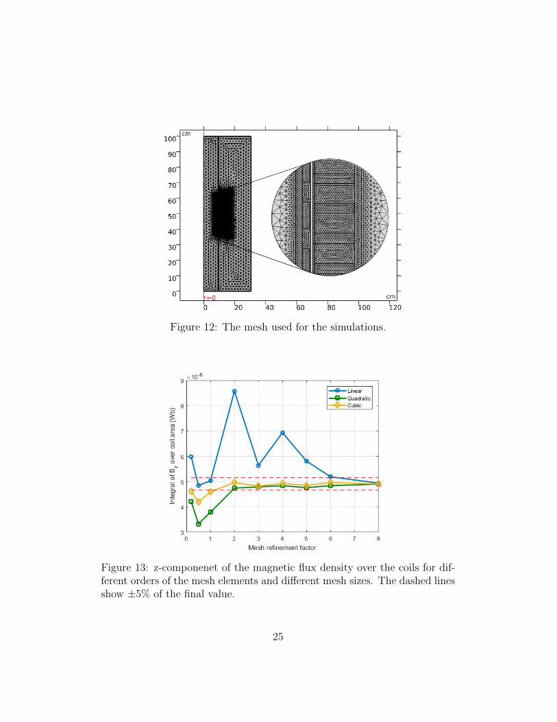
Figure 12: The mesh used for the simulations.

Figure 13: z-componenet of the magnetic flux density over the coils for dif-ferent orders of the mesh elements and different mesh sizes. The dashed linesshow ±5% of the final value.

25

3.2 Simulink: Electrical circuit model

The induced voltage from each coil group was exported from COMSOL toSimulink. The generator is modelled as a voltage source with the voltagetime series from COMSOL in series with a resistor (with resistance set to thecoil resistance obtained from COMSOL) and an inductor with inductanceestimated from Eq.25. A full-wave rectifying circuit with a purely resistiveload is connected to the generator circuit equivalent as in Figure 8. TheSimulink model is shown in Figure 14. The load resistance is adjusted in aniterative process using a MATLAB script so that the damping (calculatedfrom the power) matches the assumed input damping. The efficiency canthen be calculated.

Figure 14: Simulink model of rectifying circuit for the generator

26

4 Prototype experiment

To ensure that the numerical model is a good representation of a real gener-ator, a small scale and simplified version of the generator was constructed.The induced voltage was measured and compared to that predicted by acorresponding COMSOL model.

4.1 Experimental set up

The translator consists of a steel cylinder with magnets placed on the outsidein two rows of 17 magnets each. A cord attached to the translator enables itto be moved vertically by hand. The stator consists of a cable wound arounda plastic tube to make the coil. A cardboard tube is fitted inside the coil tobe able to move the translator smoothly up and down. See pictures of theexperimental set up in Figure 15.

Table 1: Parameters for the experimental set up

Magnet dimensions 15x15x8 mmNumber of magnets 34 in 2 rows

Remanent flux density 1.3 TCore tube diameter 8.9 cmCore tube thickness 3 mm

Air gap 5 mmCable diameter 1 mm copper

2 mm incl. insulationCoil height 6 cmCoil width 5 mm

Coil diameter 12.3 cmNumber of turns 107

The induced no load voltage was measured with an oscilloscope. Thetranslator was pulled upwards from the bottom position (on the floor) to thetop of the tube (the translator moves from well below to well above the coil).The position of the translator was measured using a draw-wire displacementsensor. A linear fit of the position measurement was used to obtain the speed,this was then used as input in the numerical model. The motion of the small

27

Figure 15: Experimental set up. Left: Finished prototype. Right: Top showstranslator (left) and coil (right) and bottom shows the individual magnetsbeing attached to the translator.

buoy (see Figure 11) has a maximum speed of 0.62 m/s with a mean speed of0.16 m/s. Two different tests were conducted with different average speeds:0.48 and 0.89 m/s.

4.2 Numerical model

The different parts of the numerical representation of the experimental setup is shown in Figure 17. The numerical model is a 2D axisymmetric model,meaning that everything is assumed to have cylindrical symmetry. This in-cludes the magnets, which are modelled as solid rings rather than individualmagnets. A separate full 3D model was made to study the differences be-tween the two cases, considering only the steady state magnetic fields. Thetwo different geometries can be seen in Figure 16. The 3D model was usedto calculate the difference in magnet volume between the two cases. Theresulting magnetic flux in an iron tube surrounding the magnets was alsocalculated and compared for the two cases. The resulting magnetic fluxdensity and magnetic field lines are shown in Figure 18. We can see thatthe top magnets are magnetised in the negative r-direction and the bottom

28

magnets in the positive direction. The small magnets was found to have avolume of 0.84 times that of the solid magnets, while the ratio for the mag-netic flux density wass 0.85. Adjusting the remanent flux density of the solidmagnet by this factor reduces the magnetic field in the iron by the same fac-tor. Therefore, when modelling the induced voltage, B0 is multiplied by 0.85.

Figure 16: Drawn geometries using small magnets (left) and solid ring mag-nets (right).

4.3 Experimental results

The position measurement and a linear fit (using MATLAB’s built in leastsquare functionality) can be seen in Figure 19. The induced voltages obtainedfrom the measurement and from the numerical model is shown in Figure 20.The graph of the calculated voltage has been shifted so that the zero crossingbetween the peaks (when the translator is exactly in the middle of the coil)occurs at the same time as the one for the measured values. The calculatedvoltage predicts higher initial peaks before the main peaks and the secondpeak is larger and somewhat skewed compared to the measured values. Ingeneral it provides a reasonably good estimate. The effect of the differencein magnet volume is not significant, but seems to be well accounted for byadding the factor Rfac to the remanent flux density of the magnets. Figure21 shows the induced voltage for the case where the translator moves withspeed 0.89 m/s.

29

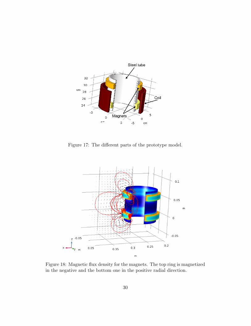
Figure 17: The different parts of the prototype model.

Figure 18: Magnetic flux density for the magnets. The top ring is magnetizedin the negative and the bottom one in the positive radial direction.

30

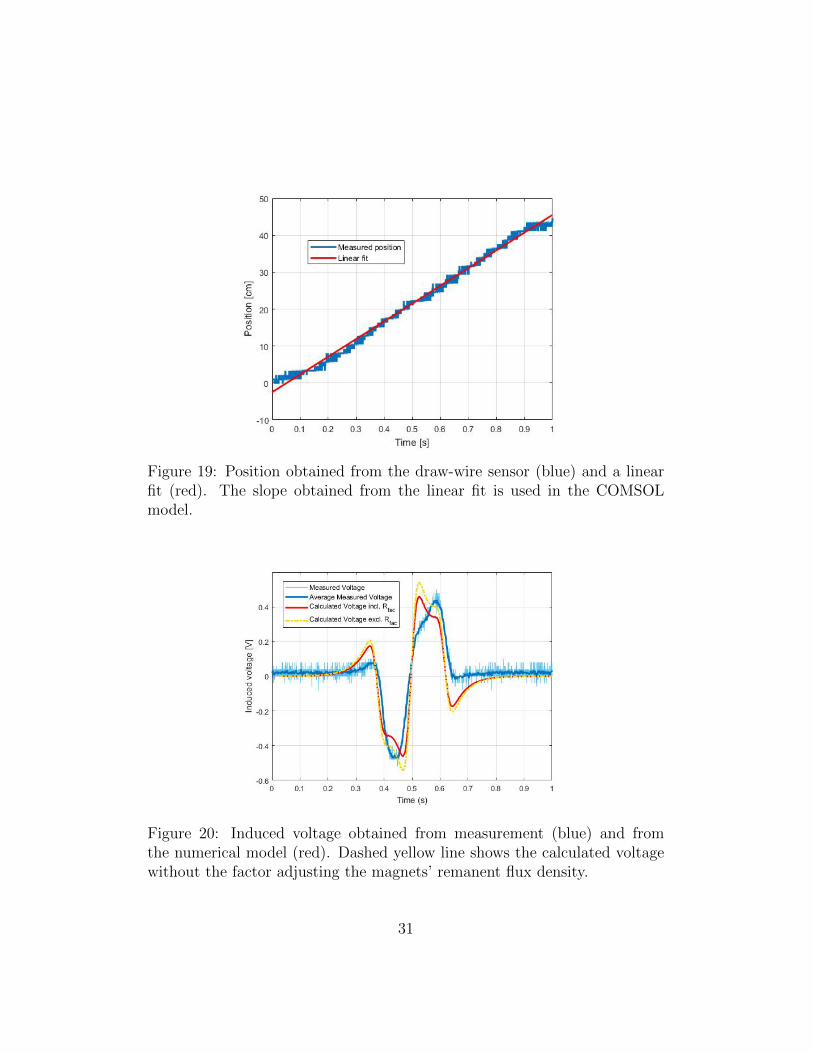
Figure 19: Position obtained from the draw-wire sensor (blue) and a linearfit (red). The slope obtained from the linear fit is used in the COMSOLmodel.

Figure 20: Induced voltage obtained from measurement (blue) and fromthe numerical model (red). Dashed yellow line shows the calculated voltagewithout the factor adjusting the magnets’ remanent flux density.

31

Figure 21: Induced voltage for the test case with speed 0.89 m/s. Blue linesobtained from measurement and the red line is the numerically calculatedvoltage.

32

4.4 Stator iron

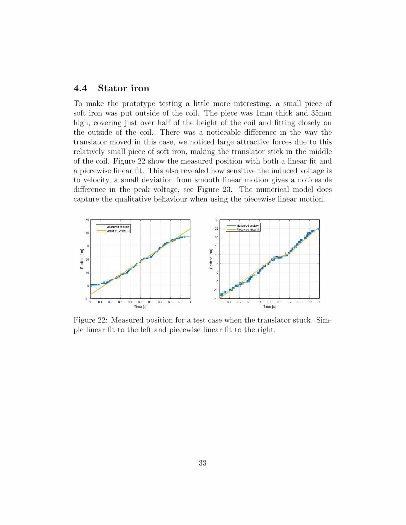
To make the prototype testing a little more interesting, a small piece ofsoft iron was put outside of the coil. The piece was 1mm thick and 35mmhigh, covering just over half of the height of the coil and fitting closely onthe outside of the coil. There was a noticeable difference in the way thetranslator moved in this case, we noticed large attractive forces due to thisrelatively small piece of soft iron, making the translator stick in the middleof the coil. Figure 22 show the measured position with both a linear fit anda piecewise linear fit. This also revealed how sensitive the induced voltage isto velocity, a small deviation from smooth linear motion gives a noticeabledifference in the peak voltage, see Figure 23. The numerical model doescapture the qualitative behaviour when using the piecewise linear motion.

Figure 22: Measured position for a test case when the translator stuck. Sim-ple linear fit to the left and piecewise linear fit to the right.

33

Figure 23: Measured and calculated induced voltage for the simple linear fiton the left and piecewise linear fit on the right.

34

5 Full size generator model

This section describes the numerical model of the suggested design for thefull scale generator and the resulting magnetic fields, power output and effi-ciency. The model is essentially the same as the one used for the experimentalverification, it is 2D axisymmetric with solid magnets when in reality it hasmany smaller individual magnets in each row. The magnets are larger com-pared to the ones used in the experimental set up and the translator has 24magnets in four rows. The parameters used can be found in Table 2 and inFigure 24.

Figure 24: Definition of the different model parameters.

5.1 Magnetic fields and induced voltage

It is the changing magnetic field that induces a voltage in the coils so it is es-sential that we know how the magnetic flux density behaves. The norm of themagnetic flux field is shown in 2D in Figure 25 and snapshots of three differ-ent instances in time in 3D is shown in Figure 26. The air gap magnetic flux

35

density can be estimated using Eq.(20). The flux density (rz-plane) in theair gap between an aligned magnet and stator tooth, assuming µfe = 1000,is found to be Ba = 0.76 T. The numerical simulation gives the maximumvalue of Ba as around 0.8 T. This occurs when the magnets and stator teethare aligned.

The current densities in the generator coils are shown in Figure 27. Atthis instance in time the translator is moving downwards so that the top andbottom coils have a negative direction for the current and the middle coilpositive. Considering the position of the magnets we can see that this is thedirection which induces a magnetic field opposing the motion according toLenz law.

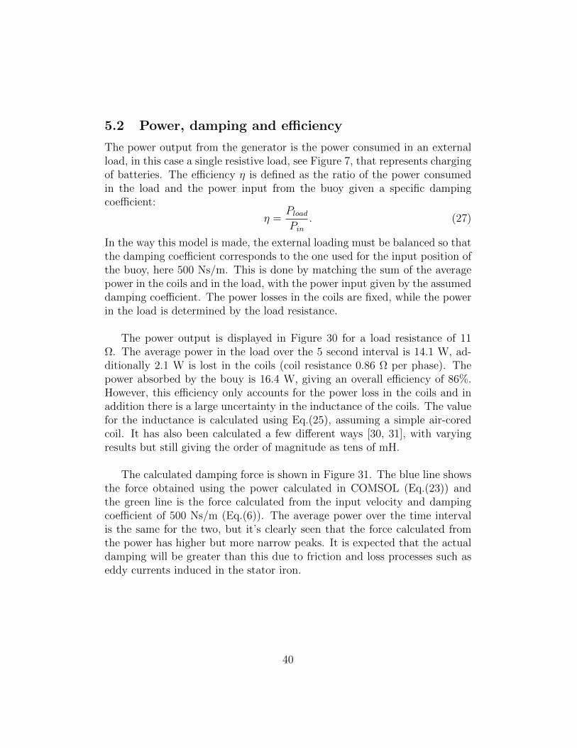
Figure 28 shows the induced voltage in the two middle coils over a 5second interval. These can be seen to be phase shifted and the highestvoltages induced for the highest velocity, c.f. Figure 11. A 60 second plot ofthe induced voltage in one coil is shown in Figure 29, where the irregular,sharp spikes of the coil voltage on the longer time scale are clearly displayed.

Figure 25: Magnetic flux density norm (T).

36

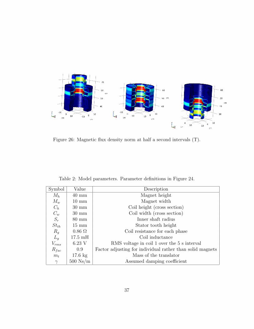
Figure 26: Magnetic flux density norm at half a second intervals (T).

Table 2: Model parameters. Parameter definitions in Figure 24.

Symbol Value DescriptionMh 40 mm Magnet heightMw 10 mm Magnet widthCh 30 mm Coil height (cross section)Cw 30 mm Coil width (cross section)Sr 80 mm Inner shaft radiusStth 15 mm Stator tooth heightRg 0.86 Ω Coil resistance for each phaseLg 17.5 mH Coil inductanceVrms 6.23 V RMS voltage in coil 1 over the 5 s intervalRfac 0.9 Factor adjusting for individual rather than solid magnetsmt 17.6 kg Mass of the translatorγ 500 Ns/m Assumed damping coefficient

37

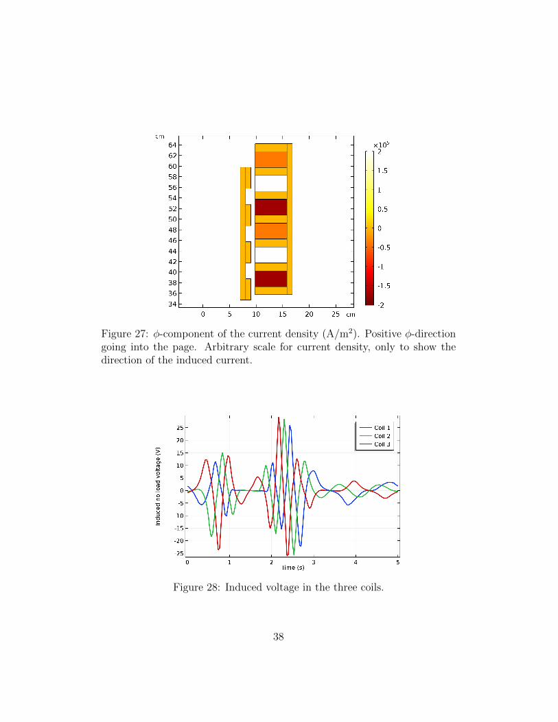
Figure 27: φ-component of the current density (A/m2). Positive φ-directiongoing into the page. Arbitrary scale for current density, only to show thedirection of the induced current.

Figure 28: Induced voltage in the three coils.

38

Figure 29: Induced voltage over a 60 second interval.

39

5.2 Power, damping and efficiency

The power output from the generator is the power consumed in an externalload, in this case a single resistive load, see Figure 7, that represents chargingof batteries. The efficiency η is defined as the ratio of the power consumedin the load and the power input from the buoy given a specific dampingcoefficient:

η =Pload

Pin

. (27)

In the way this model is made, the external loading must be balanced so thatthe damping coefficient corresponds to the one used for the input position ofthe buoy, here 500 Ns/m. This is done by matching the sum of the averagepower in the coils and in the load, with the power input given by the assumeddamping coefficient. The power losses in the coils are fixed, while the powerin the load is determined by the load resistance.

The power output is displayed in Figure 30 for a load resistance of 11Ω. The average power in the load over the 5 second interval is 14.1 W, ad-ditionally 2.1 W is lost in the coils (coil resistance 0.86 Ω per phase). Thepower absorbed by the bouy is 16.4 W, giving an overall efficiency of 86%.However, this efficiency only accounts for the power loss in the coils and inaddition there is a large uncertainty in the inductance of the coils. The valuefor the inductance is calculated using Eq.(25), assuming a simple air-coredcoil. It has also been calculated a few different ways [30, 31], with varyingresults but still giving the order of magnitude as tens of mH.

The calculated damping force is shown in Figure 31. The blue line showsthe force obtained using the power calculated in COMSOL (Eq.(23)) andthe green line is the force calculated from the input velocity and dampingcoefficient of 500 Ns/m (Eq.(6)). The average power over the time intervalis the same for the two, but it’s clearly seen that the force calculated fromthe power has higher but more narrow peaks. It is expected that the actualdamping will be greater than this due to friction and loss processes such aseddy currents induced in the stator iron.

40

Figure 30: Total power from the six coils (blue) and the power assumingγ = 500 Ns/m.

Figure 31: Damping force calculated from the power obtained from the power(red) and from the input velocity assuming γ = 500 Ns/m (blue).

41

5.3 Parameter dependence

Parametric analyses on a tubular linear generator was performed in Ref.[37].It found that pole pitch (distance between magnets), height of the stator, coilthickness and magnet thickness have the largest influence on the magnitudeof the flux through the stator iron. To find out how different parametersinfluence the average power obtained for this generator model, a numberof parametric sweeps were performed. The only design constraints are amaximum diameter of 35 cm and that the weight of the translator shouldbe 20 kg. The different magnet sizes considered were ones readily availablefrom the supplier. When actually constructing the generator, a number ofadditional criteria might need to be satisfied. The geometry, materials ordesign will likely be changed in order to accommodate for example economicalor practical aspects. For this reason, it is desirable to study the effects ofdifferent parameters and if possible identify key parameters/indicators forhigh efficiency to speed up the design process. The following sections describethe different parameters that have been studied.

5.3.1 Coil geometry

The coil area and the height of the space between the magnets have beenvaried by performing a large parameter sweep in COMSOL. 18 different caseswere then run through Simulink to find the efficiency. From this a numberof parameters were Figure 32 shows that the efficiency is very well accountedfor by using the RMS voltage from one coil divided by the coil resistance. Toget a quick estimate of the performance of the generator it is therefore suffi-cient to find and compare the RMS voltage and coil resistance only, withouthaving to run the Simulink simulation.

In the model, the available coil area determines the number of coil wind-ing turns given a specific cable size. That is, as many coil turns as possible isfitted in the available area. Increasing the number of coil windings increasesthe induced voltage linearly but the coil resistance and inductance also in-creases. To achieve a high efficiency, a balance between the two should befound. The parameter sweep showed a large variation in efficiency, the lowestefficiency being 10% while the highest was 86%. Figure 33 shows that theRMS value of the induced voltage (in one coil) and the coil resistance hasa seemingly linear dependence on the coil width. It is on the other hand

42

Figure 32: Efficiency as a function of the RMS voltage squared divided bycoil resistance.

largely uninfluenced by the coil height and the height of the space betweenthe magnets.

5.3.2 Magnet geometry

A few different magnet sizes have been tested and the RMS voltage is shownin Figure 34. It is clear that a larger magnet cross sectional area inducesa higher voltage, however larger magnets also increases the translator mass,which is restricted to 20 kg.

5.3.3 Stator iron thickness

The back iron thickness and the height of the stator teeth has been variedand the RMS voltage from one coil evaluated for the different cases. The coilresistance is constant so it is sufficient to consider only the RMS voltage. Theresult is shown in Figure 35, the stator tooth height has a clear maximum for17.5 mm while the stator back iron thickness in this range barely influencesthe induced voltage.

43

Figure 33: The coil width (far left) has a linear correlation with the RMSvoltage and coil resistance while the coil height and space between magnetsare largely uncorrelated.

5.3.4 Cable size

Having more coil turns increases the voltage linearly, however the coil resis-tance increases both with decreasing cable cross section area and the length ofthe coil. The inductance will also be affected. Using the estimate in Eq.(25),the inductance increases quadratically with the number of coil turns.

Three different cable cross sections were tested and showed that a balancebetween number of turns and coil resistance achieved the highest efficiency,see Table 3. Cost and availability will also be a factor in choosing the cables.

44

Figure 34: RMS value of the no load voltage in coil 1 for the different magnetsizes with a fitted linear function. The mass of the translator is indicated bythe colour of the dots.

Table 3: Three different sized cables used in the coils. The efficiency hereis defined as the ratio of power in the load and the power loss in the coilwindings: Pload/(Pload + Ploss).

Cable diameter (mm2) Number of turns Coil resistance (Ω) Efficiency2.5 159 1.7 0.844 128 0.86 0.8710 44 0.18 0.79

45

Figure 35: RMS voltage for different stator tooth height and stator back ironthicknesses.

46

5.3.5 Current in stator and core iron

The model has also been run with non-ideal soft iron, where the electricalconductivity σ = 1.12 × 107 S/m. This means that currents are induced inthe stator iron, see Figure 36. The effect is a slightly lower efficiency, onepercentage point, compared to the ideal material. However, the efficiency isin reality lower since the extra power loss and subsequent extra damping isnot included. Thus we cannot match the damping, rendering the simulationresults invalid. It is difficult to calculate the effect of the eddy currents,however, the stator iron for generators in general is commonly laminatedand the power loss using laminated sheets can be estimated according toEq.(22). We assume a constant frequency of 1.5 Hz for the wave motionand 1 mm thick laminates. A maximum magnetic flux density of 2.4 T wasobtained from the model and we then get

P eddyloss = 1.12× 107 S/m [(π1.5Hz)× 1mm× 2.4T]2 /6 = 239W/m3. (28)

This gives a total of 2.1 W over the volume of the iron in the stator. Con-sidering that this is the same magnitude as the resistive losses, it is notinsignificant and warrants further study.

Figure 36: Current density when including electrical conductivity of the sta-tor iron.

47

6 Discussion and conclusions

The experimental tests show close correspondence between the numericalmodel and the measured values. The factor used to compensate for the miss-ing magnet volume in the real set up compared to the model seems to be ableto account for the, albeit small, difference. However, most of the interestingbehaviour when including stator iron, several coils and the electrical circuithas not been evaluated and the accuracy of the full model cannot be fullyinferred from these experimental tests.

In the full model and electrical circuit, the power output is matched withthat expected from the assumed damping coefficient by varying the load re-sistance. The matching is done using the average value over the time interval.The simulated damping is found to be more narrowly peaked than the cor-responding assumed damping while having the same average power. This isat least in part due to the short stator length, since the translator movescompletely outside of the stator for part of the stroke. This does not havea significant effect on the average power obtained since the translator movesmuch slower at the ends of the strokes, i.e. providing less power.

However, in the experimental test there was a noticeable difference in theforce required to pull the translator past the coil with only a small pieceof stator iron wrapped around the coil. Solid support structures will be re-quired to keep the translator aligned, but the end effects might still be sosignificant that it warrants a longer stator. Adding more coils and makingthe stator longer would not adversely affect the power output, so it couldbe tested and evaluated while the translator is being built. Another optionis to include end stops or springs limiting the length of the stroke and thusreducing these nonlinear end effects while keeping a short stator. In thisproject the translator weight was limited to 20 kg. It is however not strict,the hydrodynamic modelling can simply be redone if required.

Parametric sweeps found that coil width and magnet area were most de-cisive for the induced voltage and generator efficiency. The efficiency can bewell predicted with the RMS value of the induced voltage and the coil resis-tance. Thus it is possible to use this value calculated directly in COMSOLfor optimisation purposes, rather than having to run the Simulink model eachtime as well. The power output is found to be very sensitive to design param-

48

eters, the efficiency was seen to vary between 10% and 86%. The size of thecables in the coils also influences the efficiency but can easily be optimisedwithin the model. For a given magnet size an optimal stator tooth heightwas found, while the stator back iron thickness was largely unimportant forthe efficiency.

In addition to the influence of design parameters, there are several sourcesof uncertainty. Notably the inductance used in the circuit simulations andthe effect of eddy currents in the stator iron. For the former, several differentestimates give the inductance within the same order of magnitude; tens ofmH. Variations in the inductance of this magnitude was found to change theefficiency by a few percentage points.

The currents induced in the stator iron when assuming a solid piece ofiron can be simulated using the model. However, this is not useful since theextra damping is not included and the resulting motion of the translator (andthus power output) cannot be determined. Instead, an estimate of the powerloss when using laminated sheets showed that it is of similar magnitude tothe resistive power loss in the coils and will if so be a significant source ofpower loss. Hysterisis losses can be calculated when choosing the exact ma-terials.

In conclusion, there are too many unknowns and assumptions to say ifthis design will provide the required output based on this model alone. Themodel could however be used concurrently while building the generator tocheck for example the qualitative behaviour of changing some dimensionsor materials. In general this type of model is more useful to be able toidentify important parameters of the construction, rather than providing afinal design.

49

6.1 Future research

For the next stage of the construction, the support structure, ends stops andintegration with the main buoy needs to be designed. In addition there aremany unexplored parts of the generator that are still to be investigated, forexample the exact geometries and materials used, as well as cost. Once thegenerator is constructed wave tests in the tank can be performed.

It is also possible to investigate and compare alternative PTO systems.It could for example be possible to utilise the tilting motion of the mainbuoy, inertial mass movement, this has the advantage of being completelyenclosed inside the main buoy [38] . It is uncertain whether this wouldprovide enough power and data of main buoy movement required to evaluatethis. One could also consider and test a linear-to-rotary conversion systemattached to a conventional rotary generator, for example one of the systemsin Ref.[7].

50

Acknowledgements

First and foremost I would like to thank Rafael Waters, Mohd Nasir Ayoband the Department of Electricity for the opportunity to perform this thesisproject. I would also like to specifically thank my supervisor Mohd NasirAyob for all his help and positive attitude during the project. Thanks alsoto Valeria Castellucci for your input and the magnets.

I would like to express my gratitude to my family for all the supportand encouragement, both during this project and during the past years ofstudying leading up to this thesis. I am especially thankful for the supportfrom my parents, I dedicate this thesis to you.

51

References

[1] Valeria Castellucci. “Sea Level Compensation System for Wave EnergyConverters”. PhD thesis. Uppsala University, 2016.

[2] Rafael Waters. “Energy from Ocean Waves: Full Scale ExperimentalVerification of a Wave Energy Converter”. PhD thesis. Uppsala Uni-versity, 2008.

[3] Iraide Lopez et al. “Review of wave energy technologies and the neces-sary power-equipment”. In: Renewable and Sustainable Energy Reviews27 (2013), pp. 413–434.

[4] Aamir Hussain Memon, Taib bin Ibrahim, and Perumal Nallagowden.“Design Optimization of Linear Permanent Magnet Generator for WaveEnergy Conversion”. In: 2015 IEEE Conference on Energy Conversion(CENCON). 2015. doi: 10.1109/CENCON.2015.7409561.

[5] Emre Ozkop and Ismail H. Altas. “Control, power and electrical compo-nents in wave energy conversion systems: A review of the technologies”.In: Renewable and Sustainable Energy Reviews 67 (2017), pp. 106–115.doi: http://doi.org/10.1016/j.rser.2016.09.012.

[6] Rickard Ekstrom, Boel Ekergard, and Mats Leijon. “Electrical damp-ing of linear generators for wave energy converters—A review”. In:Renewable and Sustainable Energy Reviews 42 (2015), pp. 116–128.

[7] K. Rhinefrank et al. “Comparison of Direct-Drive Power Takeoff Sys-tems for Ocean Wave Energy Applications”. In: IEEE Journal of OceanicEngineering 37.1 (2012), pp. 35–44.

[8] S. Chiba et al. “Consistent ocean wave energy harvesting using elec-troactive polymer (dielectric elastomer) artificial muscle generators”.In: Applied Energy 104 (2013), pp. 497–502.

[9] Bret Bosma et al. “Wave Tank Testing and Model Validation of anAutonomous Wave Energy Converter”. In: Energies 8 (2015), pp. 8857–8872. doi: http://doi:10.3390/en8088857.

[10] J.C.C. Henriques et al. “Design of oscillating-water-column wave en-ergy converters with an application to self-powered sensor buoys”. In:Energy 112 (2016), pp. 852–867.

52

[11] Deanelle Symonds, Edward Davis, and R. Cengiz Ertekin. “Low-PowerAutonomous Wave Energy Capture Device for Remote Sensing andCommunications Applications”. In: 2010 IEEE Energy Conversion Congressand Exposition. 2010, pp. 2392–2396. doi: 10 . 1109 / ECCE . 2010 .

5617902.

[12] Inc. Ocean Power Technologies. PowerBuoy Technology - Ocean PowerTechnologies. url: http : / / www . oceanpowertechnologies . com /

powerbuoy-technology/ (visited on Apr. 27, 2017).

[13] MBARI Monterey Bay Aquarium Research Institute. Wave-Power Power-buoy. url: http://www.mbari.org/technology/emerging-current-tools/power/wave-power-buoy/ (visited on Apr. 27, 2017).

[14] Cecilia Bostrom. “Electrical Systems for Wave Energy Conversion”.PhD thesis. Uppsala University, 2011.

[15] Avdelningen for elektricitetslara. Vagkraft - Institutionen for teknikveten-skaper - Uppsala Universitet. url: http : / / www . teknik . uu . se /

elektricitetslara/forskningsomraden/vagkraft/ (visited on Aug. 9,2017).

[16] V. Castellucci et al. “Influence of Sea State and Tidal Height on WavePower Absorption”. In: IEEE Journal of Oceanic Engineering 99 (2016),pp. 1–8. doi: 10.1109/JOE.2016.2598480.

[17] Mohd Nasir Ayob, Valeria Castellucci, and Rafael Waters. “Tidal EffectCompensation System Design for High Range Sea Level Variations”. In:Proceedings of the 11th European Wave and Tidal Energy Conference6-11th Sept 2015, Nantes, France. 2015.

[18] Tsutomu Kambe. Elementary fluid mechanics. London;Hackensack, N.J;World Scientific, 2007.

[19] M. Eriksson, J. Isberg, and M. Leijon. “Hydrodynamic modelling of adirect drive wave energy converter”. In: International Journal of Engi-neering Science 43 (2005), pp. 1377–1387.

[20] Liselotte Ulvgard et al. “Line Force and Damping at Full and PartialStator Overlap in a Linear Generator for Wave Power”. In: Journalof Marine Science and Engineering 4 (81 2016). doi: doi:10.3390/jmse4040081.

[21] David J. Griffiths. Introduction to Electrodynamics. Pearson EducationInc., 2008.

53

[22] Goran Jonsson. Tillampad ellara. Forsta upplagan. Lund: Teach Sup-port, 2015.

[23] Thomas S. Parel et al. “Optimisation of a tubular linear machine withpermanent magnets for wave energy extraction”. In: COMPEL: TheInternational Journal for Computation and Mathematics in Electricaland Electronic Engineering 30.3 (2011), pp. 1056–1068. doi: 10.1108/03321641111110997.

[24] K. Nilsson, O Danielsson, and M. Leijon. “Electromagnetic forces in theair gap of a permanent magnet linear generator at no load”. In: Journalof Applied Physics 99 (034505 2006). doi: 10.1063/1.2168235.

[25] Nathan Michael Tom. “Design and Control of a Floating Wave-EnergyConverter Utilizing a Permanent Magnet Linear Generator”. PhD the-sis. University of California, Berkeley, 2013.

[26] R. Vermaak and M. J. Kamper. “Design Aspects of a Novel TopologyAir-Cored Permanent Magnet Linear Generator for Direct Drive WaveEnergy Converters”. In: IEEE Transactions on Industrial Electronics59.5 (2012), pp. 2104–2115. doi: 10.1109/TIE.2011.2162215.

[27] Boel Ekergard et al. “Experimental results from a linear wave powergenerator connected to a resonance circuit”. In: WIREs Energy Environ2 (2013), pp. 456–464. doi: 10.1002/wene.19.

[28] J.K.H. Shek et al. “Reaction force control of a linear electrical generatorfor direct drive wave energy conversion”. In: IET Renewable PowerGeneration 1 (1 2007).

[29] M. Eriksson et al. “Wave power absorption: Experiments in open seaand simulation”. In: Journal of Applied Physics 102 (084910 2007).doi: http://dx.doi.org/10.1063/1.2801002.

[30] Boel Ekergard, Rafael Waters, and Mats Leijon. “Prediction of theInductance in a Synchronous Linear Permanent Magnet Generator”.In: Journal of Electromagnetic Analysis and Applications 3 (2011),pp. 155–159. doi: 10.4236/jemaa.2011.35025.

[31] John E. Lane et al. Magnetic Field, Force, and Inductance Computa-tions for an Axially Symmetric Solenoid Magnetic Field, Force, and In-ductance Computations for an Axially Symmetric Solenoid. NASA/TM-2013-217918. 2001.

54

[32] J. N. Reddy. An introduction to the finite element method. 3rd ed.Boston: McGraw-Hill, 2006.

[33] Jeong-Man Kim et al. “Design and analysis of tubular permanent mag-net linear generator for small-scale wave energy converter”. In: AIPAdvances 7.5 (2017), p. 056630. doi: 10.1063/1.4974496.

[34] Joseph Prudell et al. “A Permanent-Magnet Tubular Linear Generatorfor Ocean Wave Energy Conversion”. In: IEEE TRANSACTIONS ONINDUSTRY APPLICATIONS 46.6 (2010).

[35] M. G. Park et al. “Electromagnetic Analysis and Experimental Testingof a Tubular Linear Synchronous Machine With a Double-Sided AxiallyMagnetized Permanent Magnet Mover and Coreless Stator Windingsby Using Semianalytical Techniques”. In: IEEE Transactions on Mag-netics 50.11 (2014), pp. 1–4. doi: 10.1109/TMAG.2014.2323957.

[36] V. DelliColli et al. “A Tubular-Generator Drive For Wave Energy Con-version”. In: IEEE Transactions on Industrial Electronics 53.4 (2006),pp. 1152–1159.

[37] A. Pirisi, G. Gruosso, and R. E. Zich. “Novel modeling design of threephase tubular permanent magnet linear generator for marine applica-tions”. In: 2009 International Conference on Power Engineering, En-ergy and Electrical Drives. 2009, pp. 78–83. doi: 10.1109/POWERENG.2009.4915209.

[38] Jeffrey T. Cheung. Frictionless Linear Electrical Generator for Har-vesting Motion Energy. 2004.

55