Dept. for Speech, Music and Hearing

Quarterly Progress andStatus Report

Numerical simulations ofpiano strings

Chaigne, A. and Askenfelt, A.

journal: STL-QPSRvolume: 33number: 4year: 1992pages: 051-072

http://www.speech.kth.se/qpsr

STL-QPSR 411992

NUMERICAL SIMULATIONS OF PIANO STRINGS*

Antoine Chaipe** 6 Anders Askenfelt

Abstract

Thefirst attempt to generate musical sounds by solving the equations of vibrating strings by means of Finite Difference Methods (FDM) was made by Hiller & Ruiz (].Audio Eng.Soc. 19, pp. 462-472, 19711. It is shown here how their numerical approach and the underlying physical model can be improved in order to simulate the motion of the piano string with a high d e g e e of realism. Starting from the fundamental equations of a damped, stlff string interacting with a nonlinear hammer, a numerical finite difference scheme is derived, from which the time and spatial dependence of string displacement, velocity, and interacting force between hammer and string, as well as the force acting on the bridge, are computed in the time-domain. The strength of the model is illustrated by comparisons between measured and simulated piano tones. After this verification of the accuracy of the method, the model is used as a tool for systematically exploring the influence of string stiffness, relative strikin,~ position, and hammer-string mass ratio on string waveforms and spectra.

INTRODUCTION

The vibrational properties of a musical instrument - like any other vibrating struc- ture - can be described by a set of differential and partial differential equations de- rived from the general laws of physics. Such a set of equations, which define the instrument with a higher or lesser degree of perfection, is often referred to as a physical model. Due to the complex design of the traditional instruments, which in most cases also include a nonlinear excitation mechanism, no analytical solutions can, however, be expected from such a set of equations. Consequently, it is necessary to use numerical methods when testing the validity of a physical model of a musical instrument.

Once the numerical difficulties have been mastered, a simulation of a traditional instrument by a physical model means that the influence of step-by-step variations of significant design parameters like string properties, plate resonances, and others, can be evaluated. Such a systematic research method could hardly be achieved when working with real instruments, not even with the assistance of skilled instrument makers. In the future, it is hoped that advanced physical models, which reproduce the performance of traditional instruments with high fidelity, can be used as a tool for Computer-Aided-Lutherie (CAL).

Various numerical methods have been used extensively for many years in other branches of acoustics, for example in underwater acoustics where the goal is to solve the elastic wave equation in a fluid (Stephen, 1990). In musical acoustics, it is of great value to obtain a solution directly in the time-domain, since it allows us to listen to the computed waveform directly, and judge the realism of the simulation. Among the large number of numerical techniques available, Finite Difference Methods

'This article is submitted for publication in the Journal of the Acoustical Society of America. **Signal Department, Telecom Paris, 46 rue Barrault 75634 Paris Cedex 13, France.

STL-QPSR 411 992

(FDM) are particularly well-suited for solving hyperbolic equations in the time-do- main (Mitchell & Griffiths, 1980). For systems in one dimension, like the transverse motion of a vibrating string, the use of FDM leads to a recurrence equation which simulates the propagation along the string (Chaigne, 1992). The generality of FDM makes it possible to also use them for solving problems in two and three dimensions. The main practical limit then is set by the rapidly increasing computating time.

Historically, Hiller & Ruiz (1971) were the first to solve the equations of the vi- brating string numerically in order to simulate musical sounds. The model of the piano string and hammer used by these pioneers was, however, rather crude in view of the improvements in piano modeling over the last two decades (Suzuki & Nakamura, 1990). For example, the crucial value of the contact duration between hammer and string, in reality being a result of the complex hammer-string interac- tion, was set beforehand as a known parameter.

Some years later, Bacon & Bowsher (1978) developed a discrete model for the struck string where the hammer was defined by its mass and its initial velocity. Displacement waveforms were computed for both hammer and string at the contact point. Their model can be regarded as the first serious attempt to achieve a realistic description of the hammer-string interaction in the time domain. However, several effects were not modeled in detail. The damping was included as a single fluid (dashpot) term, and the stiffness of the string was neglected. The model assumed further a linear compression law of the felt. From a numerical point of view, no at- tempts were made to investigate stability, dispersion and accuracy problems.

More recently, Boutillon (1988) made use of finite differences for modeling a pi- ano string without stiffness, assuming a nonlinear compression law for the felt. He investigated, in particular, the hammer-string interaction for two notes, in the bass and mid range, respectively.

In all three papers mentioned, the numerical velocity, i.e., the ratio between the discrete spatial and time steps, was set equal to the physical transverse velocity of the string. It has been shown that this particular choice is possible for an ideal string only, and that the numerical scheme becomes unstable if stiffness, or nonlinear ef- fects due to large vibration amplitudes, are taken into account in the model (Chaigne, 1992).

At about the same time, Suzuki (1987) presented an alternative for simulating the motion of hammer and string, using a string model with lumped elements struck by a hammer with a nonlinear compression characteristic. He investigated, in particu- lar, some details of the hammer-string interaction, and the efficiency in the energy transmission from hammer to string. The effect of string inharmonicity was taken into account in a simplified manner by slightly modifying the values of the lumped string compliances.

In a recent paper, Hall (1992) made use of another approach for simulating a stiff string excited by a nonlinear hammer, which he named a standing-wave model. His method can be regarded as a semi-numerical approach, since it partially makes use of analytical results. By this method, he investigated systematically the effects of step by step variations of hammer nonlinearity and stiffness parameters, among other things.

Our study presents numerical simulations of piano strings in the time domain with particular emphasis on the transients, closely connected with the hammer- string interaction. In comparison with the earlier studies mentioned above, the pre-

STL-QPSR 411992

sent model has the feature of modeling the piano string and hammer as closely as possible to the basic physical relations: our model is entirely based on finite differ- ence approximations of the continuous equations for the transverse vibrations of a damped stiff string struck by a nonlinear hammer. The blow of the hammer is repre- sented by a force density term in the wave equation, distributed in time and space, and the damping is frequency-dependent.

The performance of the model has been evaluated for a large number of cases by observing fundamental quantities like the string waveforms and corresponding spec- tra, the interacting force between hammer and string, and the force exerted by the string on the bridge, for different combinations of hammer and string parameters.

The presentation is organized as follows. In Section I, the continuous model for the damped stiff string is briefly reviewed, with regard to the wave equation, and to the equations governing the hammer-string interaction. In Section 11, it is shown how this theoretical background can be put into a discrete form for time-domain sim- ulations, and a few first examples of the capabilities of the model for representing propagation phenomena in time and space are given. The aspects of numerical stability, dispersion and accuracy, are not developed here, but can be found in a pre- vious paper by Chaigne (1992). The only practical numerical question addressed in this section is the selection of the appropriate number N of spatial steps as a function of the fundamental frequency fl of the string, for a given sampling frequency fee

Section I11 presents systematic comparisons between simulations obtained with our model and experimental waveforms previously obtained from real piano strings by Askenfelt & Jansson (1988; 1993). The comparisons include representative notes of the piano in the bass, mid and treble register, played at different dynamic levels, and with different hammers.

In Section IV, the numerical model is used for a systematic exploration of some of the hammer-string parameters and their influence on string waveforms and spectra. The parameters included were: relative striking position, hammer-string mass ratio, and string stiffness, which all have in common that they have not been systematically studied previously, and that their exact values appear to be crucial for piano design.

I. THEORETICAL BACKGROUND

A. Wave propagation on a damped stiff string The present model describes the transverse motion of a piano string in a plane per- pendicular to the soundboard. The vibrations are governed by the following equa- tion:

a Z Y 2 a 2 y , a 4 y a y a 3 y - = C ,-&C -- b , - + b,; + f ( x , x , , , t ) a t 2 a x a x a t a t

in which stiffness and damping terms are included. The stiffness parameter is given by:

It has been shown that this stiffness term, which is the main cause of dispersion in piano strings, especially in the lowest range of the instrument, could strongly affect

the perceived attack transient. In the waveform, the dispersion gives rise to a -precursor which precedes the main pulses (Podlesak & Lee, 1988).

The two partial derivatives of odd order with respect to time in Eq. (1) simulate a frequency-dependent decay rate of the form

As a consequence, the decay times of the partials in the simulated tones will decrease with frequency, as can be observed in real pianos, see, for example, Meyer & Melka (1983). It must be pointed out that this simplified formula yields a smooth law of damping which is only a fair approximation of the reality. The constants bl and b3 in Eq. (3) were derived from experimental values through standard fitting procedures, and it is assumed that these empirical laws accounts globally for the losses in the air and in the material itself, as well as for those due to the coupling to the soundboard. No attempts were made towards an accurate modelling of each individual physical process that causes energy dissipation in the strings.

The model does not include the mechanisms which give rise to two different decay times in the piano tone, "prompt sound" and "after sound" (Weinreich, 1977). This effect is mainly due to string polarization, differences in horizontal and vertical soundboard admittance, and "mistuning" within a string triplet.

The force density term f (x, xo , t) in Eq.(l) represents the excitation by the hammer. This excitation is limited in time and distributed over a certain width. It is assumed that the force density term does not propagate along the string, so that the time and space dependence can be separated

From a physical point of view, it is clear that the dimensionless spatial window

g(x,xo) accounts for the width of the hammer. Within the context of numerical analysis, it is interesting to notice that the use of such a smoothing window elimi- nates the unwanted artefacts that occur in the solution when the excitation is concen- trated in a single point, and consequently introduces strong discontinuities in the computed waveform.

The density term f , (t) is related to the time history of the force F, ( t ) exerted by the hammer on the string by the following expression:

where the length of the string segment interacting with the hammer is equal to 2 8x.

B. Initial and boundary conditions

For the struck string, it is now well known that the force F, (t) is a result of a nonlin- ear interaction process between hammer and string (Suzuki & Nakamura, 1990; Hall & Askenfelt, 1988). In our model, the motion of the string starts at t=O as the hammer

STL-QPSR 411992

with velocity V H ~ makes contact with the string at the striking position xo. It is as-

sumed that F, (t) is given by a power law (Hall, 1992)

P F, (1) = ~ l r l ( t ) - y ( x 0 . t j Eq. ( 6 )

where the displacement q(t) of the hammer head is given by

and where the stiffness parameters K and p of the felt are derived from experimental data on real piano hammers. The losses in the felt are neglected.

In the computer program, the interaction process ends when the displacement of the hammer head becomes less than the displacement of the string at the center of the contact segment (xo). This yields, among other things, the contact duration be- tween hammer and string.

In the series of numerical experiments presented in Secs. I11 and IV, the string is assumed to be hinged at both ends, which corresponds to the following four bound- ary conditions (Fletcher & Rossing, 1991):

y(O,t)= y ( L , t ) = 0

and

These boundary conditions do not correspond strictly to the string terminations in real pianos, and will be reconsidered in a future work.

The continuous model of piano strings developed in this section forms the basis of our numerical model. Emphasis will now be put on the computational methods used for solving the equations, and the obtained algorithms will be discussed.

11. TIME-DOMAIN SIMULATIONS

A. String model The equations of motion for the string and hammer presented in Section I are formu- lated in discrete form using standard explicit differences schemes centered in space and time (Mitchell & Griffiths, 1980). The main variable is the transverse string dis-

placement y(x,t) which is computed for the discrete positions x, = iA x, and at discrete

time steps t, = nAt . Values of the hammer position ~ ( t ) are computed, using the same time grid and the same increment A t . In the subsequent parts of the paper, the following simplified notations will be used for convenience

In a second stage, the velocity and acceleration of the hammer of each discrete point of the string are derived from the corresponding displacement values by means of finite differences centered in time. Finite differences centered in space are used for computing the force transferred from one segment of the string to its

STL-QPSR 4/1992

At time t=At (n=l), the hammer displacement is given by

shown in the figure cover the range of a grand piano. In practice, the computation will be made at a lower sampling rate (say fe = 16 kHz) for notes with fundamental frequency below 100 Hz, in order to limit N to an 1000

At that time, Eq. (10) cannot yet be used for computing the string displacement, since four time steps are involved in the general recurrence equation. However, y(i,l) can be estimated by the approximated Taylor series (Mitchell & Griffiths, 1980):

y(i,l) = [y(i+l,O) + y(i-l,O)l/2 Eq. (16)

acceptable value. The synthesized signals will be then interpolated by a factor 2 or 3 and played back at a standard sampling rate. At the other end, over- loo

8 sampling will be necessary for the highest notes of 2 V1

the instrument (typically for f1 greater than 1 kHz, g lo

i.e., for note C6 and above), since truncation errors x

may appear in the solution for too small values of 2 N. In this range, the computations were made with 1

Thus, the force exerted by the hammer on the string becomes:

' ( c ) UNSTABLE

This enables us to compute a first estimate of the displacement y(i,2). In order to limit the time and space dependence for n=2, a simplified version of Eq. (10) is used, where the stiffness and damping terms are neglected. This yields:

10

. (b'k 100 1000 10000 a sampling rate of 64 kHz, or even 96 kHz for note FUNDAMENTAL FREQUENCY (HZ)

C7, and the signals were played back after low-pass Fig. I , Number of maximum spatial filtering and decimation. steps Nmax as a function of the

fundamental frequency f1 of the B. Modeling the initial and boundary conditions string for different values of the

stiffness parameter E. a ) &=lo-8; b) At time t=O (n=O), the hammer velocity is assumed E=10-6,, c) E=10-4, The sampling to be equal to VHO, and its displacement and the frequency isfe=48 k ~ z . force exerted on the string are taken equal to zero. For the sake of simplicity, only the simplest case, where the string is assumed to be at rest at the origin of time, will be presented below. Note, however, that the model can handle any initial condition. With the string at rest at t=O

Similarly, the hammer displacement q(2) is given by:

and the hammer force is now written:

F(2) = K l q(2) - y(i0,2) I P Eq- (20)

At this stage, one may ask if it is fully justified to compute the displacements in Eqs. (18) and (19) at time n=2 using the value of the force at time n=1, i.e., with a

STL-QPSR 411992

time delay equal to At. This follows from the implicit form of Eq. (20), which re- quires the values of the displacements in order to compute the hammer force.

Normally, the effects of this approximation can be neglected, provided that the sampling frequency is sufficiently high. In that case, only the high-frequency content of the synthesized signal will be affected by the delay, and the influence on the com- putations will be small. An accurate estimation of the effect can be obtained by iterating the procedure described above, and calculating a second estimate of the dis- placements using Eq. (20), which in turn leads to a more accurate estimate of the hammer force. This procedure can be repeated until no significant differences between successive results are observed. In our simulations, the algorithm converged rapidly and the differences between the first and second estimates for dis- placements and forces were never greater than 1% in the worst cases. It was therefore decided to calculate only the first estimate of the variables, in order to limit the computational time.

Once the values of the displacements are known for the first three time steps, it is possible to start using the general recurrence formula given in Eq. (lo), where the future displacement y(i,n+l) is computed assuming that the present force F(n) is known. The hammer leaves the string when

q(n+l) < y(io,n+l) Eq. (21)

after which time the string is left to free vibrations. In this case, Eq. (10) still applies, but the force term is removed.

An attractive feature of the method is $ - that there is no need to assume that the z g 0.5

string initially is at rest. The force 3 density term f(x,xo,t) can be introduced 2 2 - 0 5 a at any time in the wave equation, - u -1 1 3 0 10 20 30 40 50 :O whatever the vibrational state -of the h

ma string. Thus, the model makes it pos-

Fig 2. illustration of a repetition of a note. sible to simulate not only isolated tones, Computed string displacement (at 40 mm from the but also a musical fragment with realis- hammer, bridge side). First blow of hammer at t=O tic transitions between notes (see Fig. 2). with string initially at rest, followed by a repeated This feature is not available in blow at t=32 ms with string in motion. commercial synthesizers.

As for the boundary conditions, the numerical expressions corresponding to hinged ends case in Eq. (8) are straightforward and yield:

y(0,n) = 0 and y(N,n) = 0 Eq. (22)

y(-l,n)=-y(1,n) and y(N+l,n)=-y(N-lfn)

If the load of the soundboard at i=N is modeled by a frequency dependent admit- tance, then the second condition in Eq. (23) can conveniently be replaced by the discrete form of the appropriate differential equation. This refinement has already been successfully applied to the guitar (Chaigne, 1992).

The conditions given in Eq. (23) are important for deriving specific recurrence equations for the points i=l and i=N-1 which are close to the string terminations. Due to the stiffness term, Eq. (1) is of the fourth-order in space, and thus the recurrence equation for the point i will depend on the vibrational state of points i-2 to i+2. Therefore, it is necessary to know the values of the displacements y(-l,n) and

STL-QPSR 411992

computations. Examples of waveforms generated by the model for note C4 are shown in Fig. 3.

LRIWC. STRIKING POINT HAMMER FORCE 1 mmml 0 !r.'1

- 1 0 5 - 10 0 5 rn. 10

3 m/n

0

-3 0 5 nu I 0 5 mr

WRING, BRIDGE SIDE

Fig. 3. Computed waveforms for piano string C4 at four positions. Bridge side (a ) string displacement (at 40 mmfrom the hammer), (b) string velocity. Agraffe side (c) string displacement (at 40 mm from the hammer); ( d ) string velocity. Striking point (e) string displace- ment, (f) string velocity. (g) hammer force. Bridge (h) force transmitted to the bridge.

STRING. ACRAFFE SIDE

a A H B

Fig. 4. Simulated velocity profile of a piano string (C4) during the first 4 ms afier the blow. The time step between successive plots is 62.5 ps. The string terminations are indicated by A (agraffe) and B (bridge), and the striking point by H (hammer).

A great advantage of using a fi- nite difference method is that each physical quantity (displacement, ve- locity, force) is directly available for

all discrete points at each time step. In this way, it becomes straightforward to plot the vibratory state of the string at successive instants, in order to obtain a view of the wave propagation along the siring. This feature is illustrated in Fig. 4, which shows the velocity profile of a C4 string during the first 4 ms after the blow of the hammer. In particular, the propagating wave front and its reflexion at the bridge can be clearly seen. Similar plots of the wave propagation on a piano string have been presented by Suzuki (1987); however, using a string model with lumped elements.

111. COMPARISON BETWEEN REAL AND SIMULATED PIANO TONES

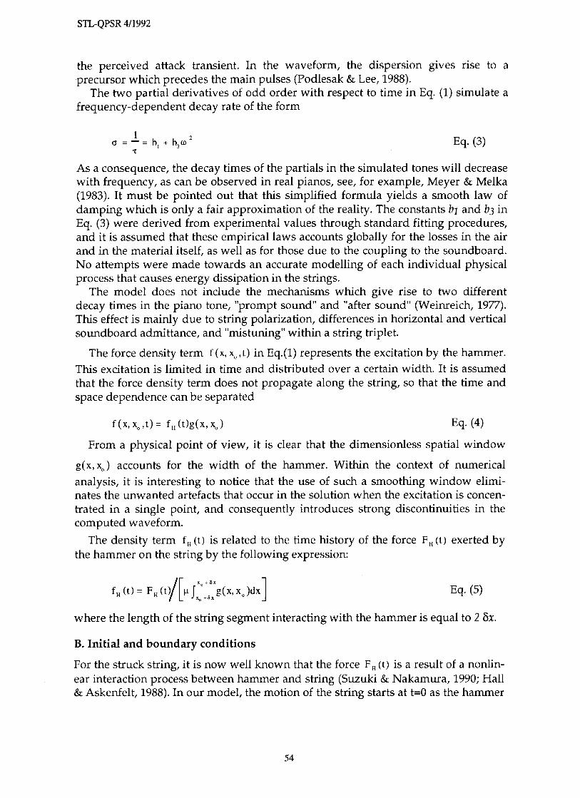
A. Bass, mid, and treble The performance of the numerical model was evaluated by comparing simulated string and hammer waveforms with previously measured signals in real pianos Askenfelt & Jansson, 1988; forthcoming). Fig. 5 shows a comparison between the simulated and observed string velocities close to the hammer (40 mm from the striking point towards the bridge) for a treble (C7), mid range (C4), and bass note (C2) respectively. It can be seen that the discrete modeling is able to reproduce the

STL-QPSR 411992

waveforms quite well over the whole register of the piano, including the details of the attack transients. Small discrepancies which can be observed in the actual timing relations between the pulses are mostly due to slight differences in observation points.

-2.51 . ' I m ' ' ' . . Y STRING L W A C l

ms Fig. 5. String velocity at the bridge side of the striking point (40 mm from the Fig. 6. Simulated hammer forces cor- hammer) for a bass, mid, and treble note responding to Fig. 5. Initial hammer velo- (C2 - C4 - C7), played mezzo forte; city V H ~ = 2.5 m/s. measured (hl l line) (Askenfelt & lansson, (2 988), and simulated (dashed).

In the C2-example, the agraffe reflection during string contact (the first negative pulse) is not modelled accurately. This discrepancy is likely due to either a non-rigid string termination at the agraffe in the real piano, or an interference with reflections from the end of the string wrapping.

The computed forces between hammer and string for the C7, C4, and C2 examples above are shown in Fig. 6. This variable is of particular interest as it determines the string spectra (Hall, 1986). The actual history of the hammer force is difficult to measure under normal conditions (Yanagisawa & Nakamura, 1984), and an indirect estimation by a measurement of the hammer retardation at the wooden hammer moulding is normally the closest alternative (Askenfelt & Jansson, 1991). The simu- lations emphasize the strong effect of the reflections from the agraffe during hammer string contact, clearly seen in the C4 and C2-examples. Each reflection results in a temporary increase in interacting force, corresponding to a downward impulse on the hammer. As discussed by Hall (1987), these reflections are one of the major mechanisms of hammer release.

The peak forces in these examples at mezzoforte level were about 40,13, and 16 N, for strings C7, C4, and C2, respectively. The high value for the C7- example is due to the pronounced nonlinearity of the treble hammers (in this case p=3.0). The hammer- string contact durations obtained in the simulations were 0.6 ms (C7), 1.9 ms (C4) and 3.25 ms (C2), respectively, which is in close agreement (within 6%) with the experimentally observed values (0.6,2.0,3.1 ms).

STL-QPSR 411992

B. Dynamic level One of the most important control parameters for the piano player is the initial hammer velocity VHO. By varying this parameter in our nonlinear physical model,

both the level and frequency content 1 .o

IV of the simulated tones will change, _ like in real pianos. This ability of the

o - model is illustrated in Fig. 7 which I v l4 _ shows a comparison of measured and

-1.0 . simulated waveforms of the string 1.0 I velocity for note C4 played at three

i5 2 different levels: forte, mezzo forte, and

o piano. The plots are presented on a

2 normalized amplitude scale. Like in $ -1.0 Fig. 5, the velocities were observed at

1.0 40 mm from the hammer on the bridge side. In the synthesis, the initial ham-

o mer velocities were 4.0, 1.5, and 0.5 m/s, respectively.

-1 .o Again, the simulations reproduce

Fig. 7. Comparison of string velocities at three the main features of the measured

dynamic levels; forte - mezzo forte - piano. (C4, obser- waveforms vation point at the bridge side, 40 mm from the the steepening of the initial slope and hammer). Measured waveform (fill line) (Askenfelt b general shortening of the pulses with lansson, 1993), and simulated (dashed) with initial increasing dynamic level. ~h~ major hammer velocity VHO equal to 4.0,1.5, and 0.5 m/s. difference is found in the forte-ex- ample where a complete match of the first agraffe reflections not is reached, possibly indicating a slight discrepancy in the hammer parameters between the real and si- mulated case. Also, the contribution from string stiffness is more pronounced in the measured waveform, clearly visible in the forte-example as a "ripple" with increasing amplitude at the end of the first period (see also Section IV-A).

t The calculated hammer forces corresponding to the three examples at forte, mezzo

o forte, and piano levels in Fig. 0 1 m8 8? 3 7 are shown in Fig. 8(a). The yy=. simulations show, in partic-

ular, how the nonlinear stiff- ness narrows the force pul-

0 o I m8 2 ses as the initial hammer ve-

locity is increased. The peak force increased from about 2

0.5 N at piano to 22 N at forte.

\ I The normalized plots in Fig. 0

o I nu 2 8(b) illustrate clearly how

Fig. 8. Simulated hammer forces for note C4 at three dynamic the waveform of the hzunmer- levels (f- mf - p ) correspond-ing to Fig. 7; (a) absolute values string force sharpens as the in N ; (b) normalized.

STL-QPSR 411992

1m (about +15%), possibly indicating a small error in the estimation of the hammer parameters.

0 o "' V V . SYSTEMATIC VARIATIONS OF HAMMER AND

STRING PARAMETERS

B J O In Section 111, the goal was to assess the power of our numerical model in reproducing the main features of real piano strings. It

1 O 0 ma 2 was shown, in particular, how the model was able to account

20 successfully for- the influence of both initial hammer velocity and felt compression properties. These numerical simulations

I I 10 confirm the basic assumptions on the behavior of piano strings 0

0 1 - 2 developed in the past few years by several authors (see, for

Fig. 21. Simulated example, the recent paper on nonlinear modeling of piano hammer forces cones- string by Ha11 (1992)). ponding to Fig. 20 In this section, our model is used as a tool for systematically with three dr;fferenf exploring the influence of some hammer and string parameters hammers (C7H - on string waveforms and spectra. The parameters selected for C4H - C2H' striking the numerical experiments included string stiffness, hammer- note C4.

string mass ratio, and relative hammer striking position (or "striking ratio"). These parameters are relatively difficult to change experimentally, so a numerical method lends itself particularly well for this purpose, once the method has been verified to perform satisfactorily. The general procedure used here was to start from the measured values of the parameters (see Table I), and proceed by varying one parameter at a time, step by step.

A. String stiffness (ID

In Fig. 13, the string velocity waveform of a bass note (C2) is shown as the string stiffness is varied by 250%

dB:: 15 Fi compared to its nominal value (see Table I). It is seen that 0

0 2 4 6 8 1 0 kilz

the major effect of increasing the stiffness is to enhance the precursor preceding the reflection from the bridge. The example illustrates the ability of the numerical method to reproduce dispersive effects due to stiffness directly in the time-domain. In the spectra, the effect of 0 7. 4 8 OkH,10

stiffness changes was less pronounced, visible only as a slight increase in the progressive spacing of the partials. d~ 00

45

B. Hammer-string mass ratio The influence of changing the hammer-string mass ratio 0

0 2 4 6 8 1 0 kH.

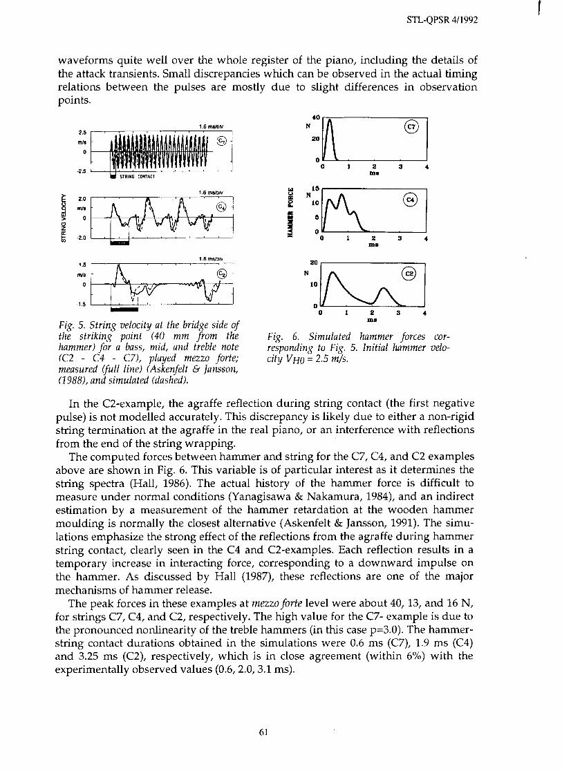
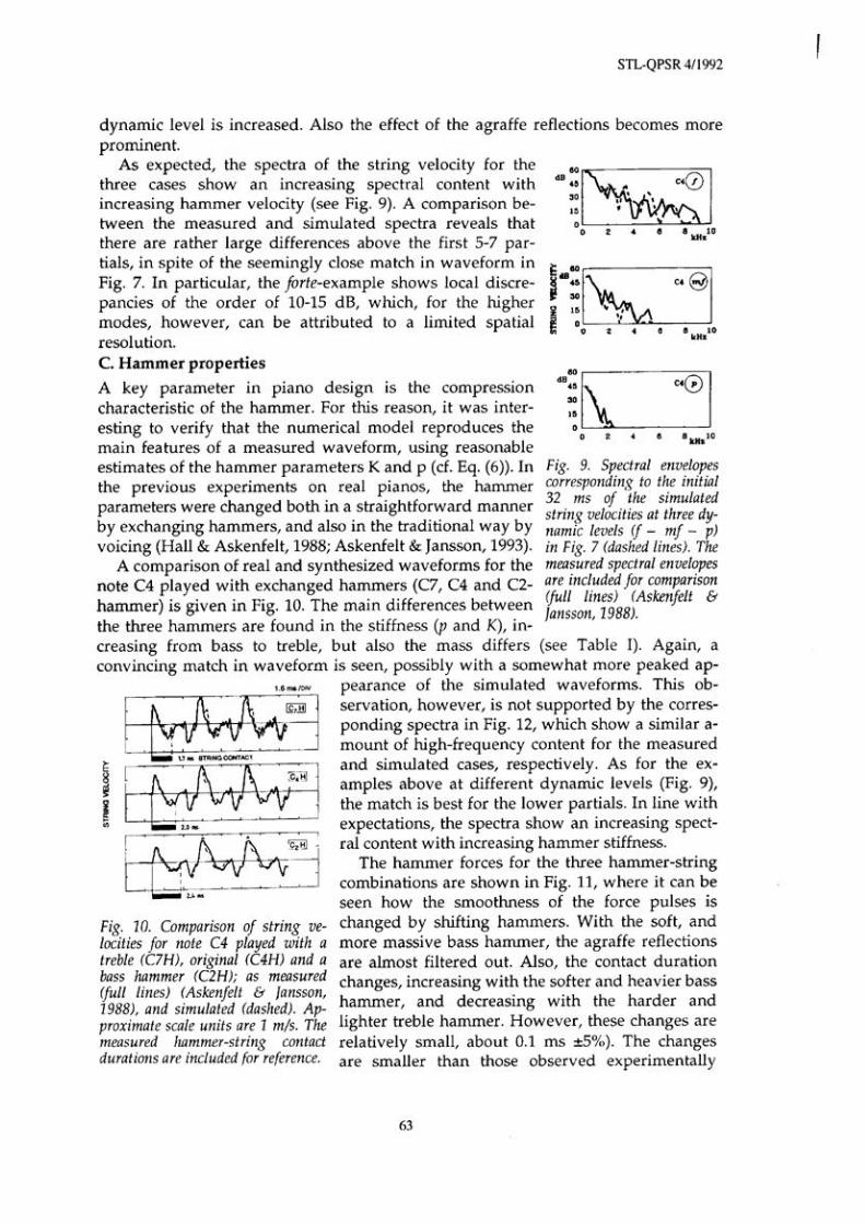
was most clearly reflected in the interacting force be- Fig. 12. Spectral envelopes tween hammer and string. Figs. 14(a) - (c) show hammer correspondin,q to the initial forces for the notes C2, C4, and C7, each note including 32 ms of thesimulated string three cases corresponding to different hammer-string velocities in Fig. 10 (dashed). mass ratios; halved, nominal and doubled respectively The measured spectral enve-

lopes are included for cam- (see Table I). It can be seen that a major effect of making (fill lines). (Hall, the hammer heavier is to increase the contact duration, 2992; Askenfelt & jansson, , and vice versa. For the notes C4 and C7, the increase is 2988).

STL-QPSR 411992

16). This is a consequence of the broadening of the string pulses, which corresponds to a lower cut-off frequency. Also, a slightly weaker fundamental could be observed for the light-hammer case.

Fig. 15(a) influence of the hammer-string mass ratio in the mid range. Simulated forces at the bridge corresponding to the C4-example in Fig. 14(b) with three different hammer-string mass ratios; light, normal, and hea y.

Fig. 15(b). Influence of the hammer-string mass ratio in the treble. Simulated forces at the bridge corresponding to the C7- example in Fig. 14(c) with three different hammer-string mass ratios; light, normal, and heavy

The corresponding examples for the C7-note with different hammer-string mass ratios (see Fig. 15(b)) show an interesting detail, in that the smoothest waveform in bridge force is obtained with the nominal value of hammer-string mass ratio. For the light hammer case, the pulses are narrow enough to just become separated, with a hint of zero displacement in between. In the heavy hammer case, the waveform be- comes more peaked and triangular, and the first pulse is considerably higher than the following. The observations are confirmed by the spectra, showing that the case with nominal hammer-string mass ratio (corresponding to a real instrument) gives the least amount of high-frequency energy. In particular, the difference compared to the light-hammer case was substantial with a clearly steeper spectral slope for the nominal case, resulting in a 10 dB level difference at 10 kHz. This is an expected re- sult, but the heavy-hammer case also gave a drop in spectral level of the same order above 8 kHz. It is an open question, whether the manufacturers are aware of the existence of a "least high-frequency ratio" for the hammer and string masses, and if this is exploited in the design. All three examples in Fig. 15(b) have been observed in measurements on real pianos, however, at different parts in the treble depending on manufacturer and instrument size.

C. Striking ratio The influence of the relative hammer striking position (striking ratio) was also in- vestigated. Fig. 17(a) shows the changes in waveform and duration of the hammer force for note C4, as the striking ratio was varied between 0.04 (1/25) and 0.24 (1/4.2). The nominal value for the C4-simulations was 0.12, which is close to the striking ratios measured for this note in real pianos (between 1/8 = 0.12 and 1/7 =

STL-QPSR 411992

1976; Hall & Clark, 1987). The overall spectral slope does not change as the striking ratio is varied.

-10 0 10 m, 20 30

Fig. 18. influence of relative hammer striking position for note C2. Simulated force at the bridge for three relative striking positions; (a) short, 0.06 (- SO%), (b) normal, 0.12, (c) lon'g, 0.24 (+ZOO%). The first and second reflec- tions from the agrafie are indicated by A1 and A2, respectively.

4 5 kHz

30

15

0 0 I 2 3 kHz

6

Fig. 19. Spectra of the simulated bridge forces in Fig. 18 for note C2 with three relative hammer striking positions; (a) short, 0.06 (1/16.7), (b) normal, 0.12 (1/8.3), and long, 0.24 W4.2). The dashed vertical lines indicate thefirst minima due to the relative striking position.

V. DISCUSSION The numerical model presented in this paper has been shown capable of reproduc- ing the characteristic features of real piano strings both in the time and frequency domain. The influence of the control parameters for the excitation of the struck string (such as initial hammer velocity and felt compression properties), discussed by sev- eral authors (Boutillon, 1988; Hall, 1992; Suzuki, 1987), has been confirmed. In addi- tion, informal listening tests have shown that the synthesized tones sound very similar to the vibrations of real piano strings, as recorded by appropriate string transducers.

The flexibility of the simulation program makes it possible to use it as a efficient tool for exploring a wide range of physical parameters, such as string stiffness, hammer-string mass ratio, and relative hammer striking position. Such a systematic exploration of the piano design, guided by a perceptual evaluation, is probably one of the major features of sound synthesis by physical modeling.

Our numerical model of the piano string is still far from complete. Among other things, the boundary conditions are modeled in a rather crude way. Work in pro- gress include an attempt to terminate the last segment of a string by a realistic load, obtained from admittance measurements at the bridge of a real piano (at the point where the actual string crosses). Pilot experiments have already been conducted with simulations of a triplet of slightly detuned C6-strings coupled by the bridge (Wogram, 1980). This approach has given significant improvements in the realism of the synthesis.

By including a modeling of the two directions of string polarization, one in paral- lel and one perpendicular to the soundboard, we expect to obtain a more realistic decay process, due to the energy exchange between the two families of modes (Weinreich, 1977). For this purpose, some preliminary measurements of the admit- tance matrix at the bridge will be necessary.

Presently, it must be admitted that the simulated tones don't mimic real piano tones convincingly when listening, a slightly disappointing fact. The essential miss- ing feature in the synthesis is in the attack component, which for a real piano tone include a strong "thump," transmitted from the whole structure of the instrument. This component is due to the shock-like excitation. A large part of the thump is transmitted to the soundboard by a longitudinal motion on the string, which pre- cedes the first transversal string pulse by 1-2 ms (mid-range), a so-called "precursor" (Podlesak & Lee, 1988). This effect can be isolated from the "sounding" part of the - - tone by damping the transversal string motion (with the hand).

Other transient components are ex- 5 m s ~ ~ ~

cited by the inertial force of the ac- ,g2 celerating hammer, as well as from the KEY BOITOM

finger force on the key, which both are transmitted to the iron plate and sound- board via the keybed and rim. An exam- ple of the attack components, as regist- ered at the bridge, is shown in Fig. 20,

removed and the hammer strikes a dum- for a case where the strings have been *

my mass- This was done in cxder to a- Fig. 20. Regstration of the acceleration at the void a masking of the attack components bridge with the strings removed and the hammer by the much stronger string vibrations. striking a dummy mass (C4, jorte, staccato- Interestingly, it appears that the partic- touch). The bridge motion starts with a per-

cussive component about 20 ms before hammer- of the attack components are dummy contad, followed by a "wave pachge" at

affected by the pianist's type of touch. about 1000 H z (due to a resonance in the key). By adding a recording of the attack Later, the motion is dominated by a mixture of

components (with damped strings) to resonances in the keybed at 700 and 250 Hz, the computer simulations, significant im- approximately. The vibration level of these pre-

and postcursors is of the same order as the bridge provements in the of the 'yn- vibrations due to string motion at pp-level. thesis were obtained. This have en- couraged us to continue the modeling of the longitudinal vibrations of the string, once the soundboard admittance at the bridge termination has been satisfactorily implemented.

ACKNOWLEDGEMENTS

Part of this work was conducted during Fall 1990, when the first author was a guest researcher at the Department of Speech Communication and Music Acoustics, Royal Institute of Technology (KTH), Stockholm, with financial support from Centre Na- tional de la Recherche Scientifique (CNRS). The project was further supported by the Swedish Natural Science Research Council (NFR), the Swedish Council for Research in the Humanities and Social Sciences (HSFR), the Bank of Sweden Tercentenary Foundation, and the Wenner-Gren Center Foundation.

STL-QPSR 411992

APPENDIX A: COEFFICIENTS OF THE RECURRENCE EQUATION FOR THE DAMPED STIFF STRING

STL-QPSR 41 1992

LIST OF VARIABLES AND SYMBOLS coefficients in the discrete wave equation damping coefficients string tension linear mass density of string

transverse velocity of string string length string mass hammer mass hammer-string mass ratio (HSMR) Young's modulus of string string stiffness parameter distance of hammer from agraffe relative hammer striking position (RHSP) force density fundamental frequency sampling frequency hammer force spatial window spatial index coefficient of hammer stiffness time index number of string segments stiffness nonlinear exponent initial hammer velocity transverse displacement of string time step spatial step hammer displacement radius of gyration of string decay rate decay time angular frequency