Embed Size (px)
Citation preview

Numerical simulations of naturalconvection around a line-source
Shihe XinLIMSI-CNRS, Orsay, France
Dep de Physique, Univ. Paris Sud, Orsay, France
Marie-Christine Duluc, Francois Lusseyran and Patrick Le QuereLIMSI-CNRS, Orsay, France
Keywords Convection, Boundary layers, Numerical analysis
Abstract External natural convection is rarely studied by numerical simulation in the literaturedue to the fact that flow of interest takes place in an unbounded domain and that if a limitedcomputational domain is used the corresponding outer boundary conditions are unknown. In thisstudy, we propose outer boundary conditions for a limited computational domain and make thecorresponding numerical implementation in the scope of a projection method combining spectralmethods and domain decomposition techniques. Numerical simulations are performed for bothsteady natural convection about an isothermal cylinder and transient natural convection around aline-source. An experiment is also realized in water using particle image velocimetry andthermocouples to make a comparison during transients of external natural convection around aplatinum wire heated by Joule effect. Good agreement, observed between numerical simulationsand experiments, validated the outer boundary conditions proposed and their numericalimplementation. It is also shown that, if one tolerates prediction error, numerical results obtainedremain at least reasonable in a region near the line-source during the entire transients. We thuspaved the way for numerical simulation of external natural convection although further studiesremain to be done for higher heating power (higher Rayleigh number).
The Emerald Research Register for this journal is available at The current issue and full text archive of this journal is available at
www.emeraldinsight.com/researchregister www.emeraldinsight.com/0961-5539.htm
NomenclatureCp ¼ specific heat of working fluid at
constant pressure (J/kg K)~C ¼ specific heat of platinum (J/kg K)D ¼ cylinder diameter (m)f ¼ unknown fieldg ¼ gravity acceleration (m/s2)i ¼
ffiffiffiffiffiffiffi21
p
�I ¼ modified identity matrixk ¼ azimuthal wave numberK ¼ maximum azimuthal wave
numbern ¼ time stepNu ¼ average Nusselt number on the
surface of isothermal cylinder
Pr ¼ Prandtl number ( ¼n/k)q ¼ heat flux (W/m2)Q ¼ heat power or heat loss rate (W)r ¼ radial distance (m)R ¼ cylinder radius (m)R0 ¼ radial position of the outer
boundary (m)Raq ¼ Rayleigh number based on heat
flux ( ¼[gbqR 4] / (lnk))RaT ¼ Rayleigh number based on
temperature difference( ¼[gbDTD 3] / (nk))
Sf ¼ r.h.s. term of discrete equation of ft ¼ time (s)
Computations have been performed at Centre d’Informatique National de l’EnseignementSuperieur (CINES) under research project lim2072.
HFF14,7
830
Received November 2002Revised July 2003Accepted December 2003
International Journal of NumericalMethods for Heat & Fluid FlowVol. 14 No. 7, 2004pp. 830-850q Emerald Group Publishing Limited0961-5539DOI 10.1108/09615530410546245
1. IntroductionAlthough external natural convection has been studied in the past (similarity solutions,experiments, etc.) (Fuji et al., 1973; Ostroumov, 1956; Schorr and Gebhart, 1970;Yosinobu et al., 1979), it is still an unexplored domain for numerical simulation, asthere have been few numerical investigations of such flows (Farouk and Guceri, 1981;Kelkar and Choudhury, 2000; Kuehn and Goldstein, 1980; Linan and Kurdyomov, 1998;Saitoh et al., 1993; Wang et al., 1990).
External natural convection takes place in an infinite fluid medium or in a fluidmedium whose size is large compared with that of the heating element. When trying tostudy external natural convection by numerical simulation, sometimes one can use avery large computational domain but most of the time one has to limit thecomputational domain to a small fluid region surrounding the heating element becauseconsidering the whole fluid medium is either impossible or too expensive. In thepioneering works (Farouk and Guceri, 1981; Kuehn and Goldstein, 1980), externalnatural convection around a horizontal cylinder is studied numerically; theNavier-Stokes equations in stream function-vorticity formulation are solved byusing finite differences method and inflow and outflow boundary conditions at anartificially placed outer boundary. For an isothermal cylinder, only local Nusseltnumber along cylinder surface and averaged Nusselt number are compared withexperimental measurements and used to assess the validity of numerical results. Later,Wang et al. (1990) revisited the same problem with the same inflow and outflowboundary conditions and pointed out that these outer boundary conditions may be onlyvalid in the steady conditions. As indicated in Saitoh et al. (1993), the outer boundaryconditions used in Wang et al. (1990) do not give the correct results includingstreamlines and Nusselt number around the cylinder and there is no benchmarksolution for this standard problem. This led Saitoh et al. (1993) to propose benchmark
T ¼ temperature (K)u ¼ radial velocity component (m/s)v ¼ azimuthal velocity component
(m/s)~V ¼ vector fieldp ¼ pressure deviation from
hydrostatic pressure (N/m2)x ¼ horizontal position (m)y ¼ vertical position (m)
Greek symbolsb ¼ coefficient of volumetric thermal
expansion (K21)D ¼ Laplace operatorDT ¼ Superheat on cylinder surface
(Tw2T0)Dt ¼ time step value1 ¼ small positive valuek ¼ thermal diffusivity of working
fluid (m2/s)
l ¼ thermal conductivity of workingfluid (W/m K)
~l ¼ thermal conductivity of platinum(W/m K)
�l ¼ 3/(2Dt)n ¼ kinematic viscosity of working
fluid (m2/s)r ¼ density of working fluid (kg/m3)~r ¼ density of platinum (kg/m3)u ¼ azimuthal position in polar systemQ ¼T 2 T0 ¼ superheat (K)
Subscripts and superscriptsk ¼ wave number in Fourier spacen ¼ time stepw ¼ cylinder wallv ¼ volumetric (per volume)0 ¼ related to initial or ambient
condition* ¼ predicted velocity field
Numericalsimulations
831
solutions to natural convection around a horizontal circular cylinder by using higheraccuracy methods (fourth-order finite differences) and a solid boundary conditionplaced at some 1,000-20,000 times the cylinder diameter. Recently, Linan andKurdyomov (1998) analytically and numerically investigated natural convectionaround a line heat source at small Grashof numbers. Solutions at far-field are knownanalytically; numerical solutions close to the line source are obtained by using finitedifferences and far-field analytical solutions as inflow boundary conditions and theyare used to determine constants involved in analytical expressions of the near-fieldsolutions. Note that these numerical simulations of external natural convection (Faroukand Guceri, 1981; Kuehn and Goldstein, 1980; Linan and Kurdyomov, 1998; Saitoh et al.,1993; Wang et al., 1990) have been entirely performed in stream function-vorticityformulation.
Although using a very large computational domain can provide benchmarksolutions to external natural convection around a horizontal cylinder, obtaining correctstreamlines and reasonable results with a relatively small computational domain andartificial outer boundary conditions still makes sense and is challenging, especially fortransient external natural convection.
Using a limited fluid region surrounding the heating element as the computationaldomain gives rise to two questions. Where should we put the external boundary of thelimited computational domain? Which kind of boundary conditions must we use on theexternal boundary that is both inflow and outflow? In order to answer these questions,we proposed artificial conditions at the outer boundary of the limited computationaldomain and developed a 2D spectral (Chebyshev collocation and Fourier Galerkin) timestepping (projection) code associated with a domain decomposition technique toperform numerical simulations of external natural convection around both anisothermal cylinder and a line-source. The Navier-Stokes equations undervelocity-pressure formulation in polar coordinates are discretized in time by asecond-order scheme of finite differences type and in space by Fourier Galerkin methodin the azimuthal direction. In the radial direction, the circular computational domain isdivided into several sub-domains of different sizes so that away from the line-sourcegrids become coarser and in each sub-domain we use Chebyshev collocation methodfor spatial discretisation. On the interfaces between sub-domains, a C 1 condition isused, i.e. functions and their first normal derivatives are imposed to be continuous. Thevelocity-pressure coupling is handled by projection method.
Apart from our earlier study (Duluc et al., 2003) only one work has been realizedunder velocity-pressure formulation (Kelkar and Choudhury, 2000). Furthermore, mostof the earlier studies are only devoted to steady external natural convection. This iswhy the present study is performed under velocity-pressure formulation and particularattention has been paid to transient external natural convection. In Duluc et al. (2003),we showed that, for the benchmark problem of natural convection around a horizontalisothermal cylinder, different outer boundary conditions yielded the same Nusseltnumber, but different flow structures. Steady temperature field near the cylinder is tosome extent insensitive to computational domain size, numerical methods and outerboundary conditions. We also showed scalings with heating power in transientexternal natural convection about a line-source. Owing to the lack of experimentalresults, no conclusion was drawn on the flow structure in Duluc et al. (2003). This iswhy we set up an experiment and measured velocity field by particle image
HFF14,7
832

velocimetry (PIV) in order to validate the numerical methods used and show thefeasibility of numerical simulation of external natural convection. The present workfocuses on the numerical methods used, numerical implementation of the outerboundary conditions proposed, flow structure of external natural convection andinfluence of computational size on flow structure. It concerns mainly transient externalnatural convection around a line-source, and deals also with steady natural convectionabout a horizontal isothermal cylinder.
The present paper is organized as follows. In the next two sections we will detail thegoverning equations of the physical problem studied and the numerical methodsproposed. We will then give a brief description of the experiments performed forvalidating the numerical methods used. Numerical results and comparison betweennumerical simulations and experiments will be discussed before drawing the finalconclusions.
2. Physical problem and governing equationsWe are interested in fluid motion around a horizontal heating cylinder of radius R(Figure 1). The cylinder could be either isothermal at a constant temperature or a thinmetal wire heated at a constant power by Joule effect. At the starting time the wire issubmitted to a step of electrical current; the fluid around the wire is heated and movesup. The working fluid (water in experiment) is considered as a Newtonian fluid ofdensity r, volumetric expansion coefficient b, thermal diffusivity k (thermalconductivity l and specific heat Cp) and kinematic viscosity n. We assume that fluid
Figure 1.External natural
convection around ahorizontal cylinder
Numericalsimulations
833

motion is two-dimensional and governed by the following Boussinesq equations(Boussinesq assumption is valid) in polar coordinates:
›u
›rþ
u
rþ
1
r
›v
›u¼ 0
›u
›tþ u
›u
›rþ
v
r
›u
›u2
v 2
r¼ 2
1
r
›p
›rþ n D2
1
r 2
� �u 2
2
r 2
›v
›u
� �2 gbðT 2 T0Þcos u
›v
›tþ u
›v
›rþ
v
r
›v
›uþ
uv
r¼ 2
1
rr
›p
›uþ n D2
1
r 2
� �v þ
2
r 2
›u
›u
� �þ gbðT 2 T0Þsin u
›T
›tþ u
›T
›rþ
v
r
›T
›u¼ kDT
ð1Þ
where
D ¼›2
›r 2þ
1
r
›
›rþ
1
r 2
›2
›u 2;
t is the time, u and v are the radial and azimuthal velocity components, p is thepressure deviation from the hydrostatic pressure and T is the temperature.
In the case of an isothermal horizontal cylinder, the computational domain,ðr; uÞ [ ½R; R0� £ ½0; 2p� and the boundary conditions on the cylinder surfaceðr ¼ RÞ are
u ¼ v ¼ 0
T ¼ Tw
(ð2Þ
In the case of a platinum wire heated by Joule effect, in order to consider the wirethermal inertia, equation (1) should be coupled with the heat conduction equation
~r ~C›T
›t¼ ~lDT þ Qv ð3Þ
where Qv, a uniform volumetric heat source, represents heat power supplied by Jouleeffect. Then the computational domains for temperature and velocity are ðr; uÞ [½0; R0� £ ½0; 2p� and ðr; uÞ [ ½R;R0� £ ½0; 2p�. Initial conditions for the problemdescribed by equations (1) and (3) are u ¼ v ¼ 0 and T ¼ T0: Boundary conditions onthe wire surface ðr ¼ RÞ are
u ¼ v ¼ 0
l›T
›r
����fluid
¼ ~l›T
›r
����wire
8><>: ð4Þ
At the outer boundary ðr ¼ R0Þ the conditions are unknown and we propose thefollowing conditions:
HFF14,7
834

n›
›rþ
1
r
� �u ¼
p
r
n›
›rþ
1
r
� �v ¼ 0
8>>>><>>>>:
ð5Þ
and
›T
›r
����R0
¼›T
›r
����R021
ð6Þ
where 1, a small positive real value, will be taken as the mesh size at r ¼ R0:Note that equation (5) is derived by assuming the balance between pressure and
friction in equation (1) and degenerating them in the radial direction (Guermond andQuartapelle, 1998). Equation (6) means that radial derivative of temperature at theouter boundary is equal to that at the first inner point. When compared with theartificial conditions used earlier at the outer boundary (Farouk and Guceri, 1981;Kelkar and Choudhury, 2000; Kuehn and Goldstein, 1980; Linan and Kurdyomov, 1998;Saitoh et al., 1993; Wang et al., 1990), equations (5) and (6) are linked neither to theinflow nor to outflow at the outer artificially placed boundary. As they do not need onlya priori knowledge of inflow and outflow at the outer boundary, they need only to beimplemented once in a code without extra tests and seem to be more convenient totransient external natural convection if they are validated.
3. Numerical methods3.1 Time discretizationEquations (1) and (3) are discretized by a second-order time stepping of finite differencetype: nonlinear terms are treated explicitly and diffusion is treated implicitly. Whenapplied to an advection-diffusion equation
›f
›tþ ~V ·7f ¼ 72f
the time scheme reads
3f nþ1 2 4f n þ f n21
2Dtþ 2 ~V ·7f n 2 ~V ·7f n21 ¼ 72f nþ1
where Dt is the time step. This equation can be cast in a Helmholtz equation for theunknown field f at time n þ 1:
72f nþ1 2 �lf nþ1 ¼ Sf
where �l ¼ 3=2Dt: By noting Q ¼ T 2 T0; equations (1) and (3) are discretized in timethen read for r , R:
~lD23 ~r ~C
2Dt
!Qnþ1 ¼ SQ ð7Þ
and for R , r , R0:
Numericalsimulations
835

kD23
2Dt
� �Qnþ1 ¼ SQ;
›unþ1
›rþ
unþ1
rþ
1
r
›vnþ1
›u¼ 0;
n D21
r 2
� �unþ1 2
2
r 2
›vnþ1
›u
� �2
3
2Dtunþ1 ¼
1
r
›pnþ1
›rþ Su þ gbQnþ1 cos u;
n D21
r 2
� �vnþ1 þ
2
r 2
›unþ1
›u
� �2
3
2Dtvnþ1 ¼
1
rr
›pnþ1
›uþ Sv 2 gbQnþ1 sin u
8>>>>>>>>>>>>>><>>>>>>>>>>>>>>:
ð8Þ
3.2 Spatial discretizationSpectral methods, known to be of infinite order provided that solutions to beapproached are regular, are used for spatial discretization. The periodicity in theazimuthal direction naturally leads us to a spatial approximation based on the Fourierseries:
f ðr; uÞ ¼XK
k¼2K
f kðrÞ exp ðikuÞ
Equations (7) and (8) are reduced to the following ð2K þ 1Þ 1D problems in r:
~l›2
›r 2þ
1
r
›
›r2
k 2
r 2
� �2
3 ~r ~C
2Dt
" #Qnþ1
k ¼ SQk ð9Þ
for r , R and R , r , R0
k›2
›r 2þ
1
r
›
›r2
k 2
r 2
� �2
3
2Dt
� �Qnþ1
k ¼SQk
›unþ1k
›rþ
unþ1k
rþ
ik
rvnþ1
k ¼ 0;
n›2
›r 2þ
1
r
›
›r2
k 2 þ1
r 2
� �unþ1
k 22ik
r 2vnþ1
k
� �2
3unþ1k
2Dt¼
1
r
›pnþ1k
›rþSuk þgb
Qnþ1k21 þQnþ1
kþ1
2;
n›2
›r 2þ
1
r
›
›r2
k 2 þ1
r 2
� �vnþ1
k þ2ik
r 2unþ1
k
� �2
3vnþ1k
2Dt¼
ik
rrpnþ1
k þSvk 2gbQnþ1
k21 2Qnþ1kþ1
2
8>>>>>>>>>>>>>>><>>>>>>>>>>>>>>>:
ð10Þ
It is interesting to note that in equation (10) Helmholtz equations of unþ1k and vnþ1
k arecoupled. The coupling is alleviated by the change of variables uþ
k ¼ uk þ ivk and u2k ¼
uk 2 ivk: Furthermore, k¼ 0; divergence free and boundary conditions lead to u0 ¼ 0 andthe momentum equation for u0 turns out to be the equation for p0.
HFF14,7
836
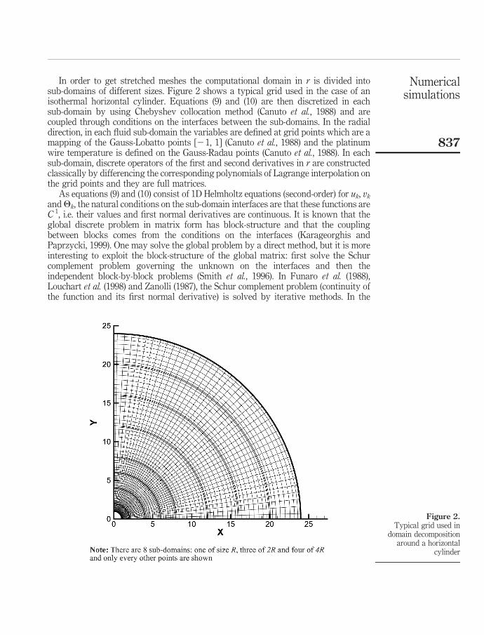
In order to get stretched meshes the computational domain in r is divided intosub-domains of different sizes. Figure 2 shows a typical grid used in the case of anisothermal horizontal cylinder. Equations (9) and (10) are then discretized in eachsub-domain by using Chebyshev collocation method (Canuto et al., 1988) and arecoupled through conditions on the interfaces between the sub-domains. In the radialdirection, in each fluid sub-domain the variables are defined at grid points which are amapping of the Gauss-Lobatto points [21, 1] (Canuto et al., 1988) and the platinumwire temperature is defined on the Gauss-Radau points (Canuto et al., 1988). In eachsub-domain, discrete operators of the first and second derivatives in r are constructedclassically by differencing the corresponding polynomials of Lagrange interpolation onthe grid points and they are full matrices.
As equations (9) and (10) consist of 1D Helmholtz equations (second-order) for uk, vk
and Qk, the natural conditions on the sub-domain interfaces are that these functions areC 1, i.e. their values and first normal derivatives are continuous. It is known that theglobal discrete problem in matrix form has block-structure and that the couplingbetween blocks comes from the conditions on the interfaces (Karageorghis andPaprzycki, 1999). One may solve the global problem by a direct method, but it is moreinteresting to exploit the block-structure of the global matrix: first solve the Schurcomplement problem governing the unknown on the interfaces and then theindependent block-by-block problems (Smith et al., 1996). In Funaro et al. (1988),Louchart et al. (1998) and Zanolli (1987), the Schur complement problem (continuity ofthe function and its first normal derivative) is solved by iterative methods. In the
Figure 2.Typical grid used in
domain decompositionaround a horizontal
cylinder
Numericalsimulations
837

present work, we used influence matrix technique or capacitance technique and a2-iteration method to solve Schur complement problem in order to guarantee theinterface conditions: the idea is to impose Dirichlet conditions on the interfaces andrelease the constraint on the first normal derivative; as there is a linear relationshipbetween the function values on the interfaces and the jump of its first normal derivativethrough the interfaces, i.e. the Schur complement, in a pre-processing step influencesmatrix (capacitance) technique that is used to construct this linear relationship byusing a complete set of canonical unit vectors of function values on the interfaces andthe Schur complement is then a inversed direct method. The solution of the globalproblem can then be obtained as follows. In the first iteration, a test Dirichlet conditionis given on the interfaces and the independent block problems are solved; in the seconditeration, the jump of the first normal derivative on the interfaces is calculated, thecorrection to test the Dirichlet condition is recovered by doing matrix-vector productbetween the inversed Schur complement and the derivative jump on the interfaces andthe right solution of the global problem is finally obtained by solving the independentblock problems with the corrected Dirichlet condition on the interfaces.
Note that in the case of a platinum wire equations (9) and (10) are coupled throughthe temperature condition at r ¼ R which implies energy conservation and takes thefollowing form:
l›Qk
›r
����fluid
¼ ~l›Qk
›r
����wire
ð11Þ
This condition couples the solid platinum domain with the first fluid sub-domain andcan also be considered as an interface coupling between the sub-domains. It is,therefore, part of the Schur complement of the global temperature problem.
3.3 Velocity-pressure couplingDivergence free flow field can be obtained either by Uzawa methods (Bernard andMaday, 1992; Canuto et al., 1988) or by projection method. We will detail in thefollowing the implementation of the condition (5) in the scope of a projection methodconsisting of two steps.
In the first step (prediction), we solve the momentum and energy equations (9) and(10) by dropping the divergence-free condition and using the pressure field p n insteadof pnþ1
k : We then obtain Qnþ1k and a predicted velocity field u*
k; v*k
� �which is not
divergence free. The corresponding outer boundary conditions to be used are:
›Qnþ1k
›r
�����R0
¼›Qnþ1
k
›r
�����R021
n›
›rþ
1
r
� �u*
k ¼ 2pn
k
r2
pn21k
r
n›
›rþ
1
r
� �v*
k ¼ 0
8>>>>>>>>><>>>>>>>>>:
ð12Þ
Note that the pressure field is extrapolated at the time step n þ 1:The second step consists of projecting u*
k; v*k
� �on the divergence free sub-space and
we therefore, solve for k – 0
HFF14,7
838
›
›rþ
1
r
� ��I›
›r2
k 2
r 2
� �pnþ1
k 2 pnk
r¼ 2
3
2Dt
›u*k
›rþ
u*k
rþ
ik
rv*
k
� �ð13Þ
where �I is a modified identity matrix whose first element is equal to zero in order toconsider the fact that on the wire surface u*
k ¼ 0: On the outer boundary ðr ¼ R0Þ weimpose:
pnþ1k 2 pn
k
r¼ 2
ik
rv*
k 2pn
k
rð14Þ
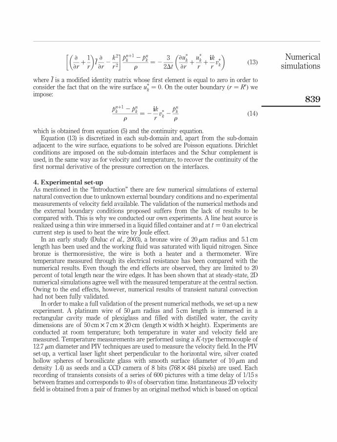
which is obtained from equation (5) and the continuity equation.Equation (13) is discretized in each sub-domain and, apart from the sub-domain
adjacent to the wire surface, equations to be solved are Poisson equations. Dirichletconditions are imposed on the sub-domain interfaces and the Schur complement isused, in the same way as for velocity and temperature, to recover the continuity of thefirst normal derivative of the pressure correction on the interfaces.
4. Experimental set-upAs mentioned in the “Introduction” there are few numerical simulations of externalnatural convection due to unknown external boundary conditions and no experimentalmeasurements of velocity field available. The validation of the numerical methods andthe external boundary conditions proposed suffers from the lack of results to becompared with. This is why we conducted our own experiments. A line heat source isrealized using a thin wire immersed in a liquid filled container and at t ¼ 0 an electricalcurrent step is used to heat the wire by Joule effect.
In an early study (Duluc et al., 2003), a bronze wire of 20mm radius and 5.1 cmlength has been used and the working fluid was saturated with liquid nitrogen. Sincebronze is thermoresistive, the wire is both a heater and a thermometer. Wiretemperature measured through its electrical resistance has been compared with thenumerical results. Even though the end effects are observed, they are limited to 20percent of total length near the wire edges. It has been shown that at steady-state, 2Dnumerical simulations agree well with the measured temperature at the central section.Owing to the end effects, however, numerical results of transient natural convectionhad not been fully validated.
In order to make a full validation of the present numerical methods, we set-up a newexperiment. A platinum wire of 50mm radius and 5 cm length is immersed in arectangular cavity made of plexiglass and filled with distilled water, the cavitydimensions are of 50 cm £ 7 cm £ 20 cm ðlength £ width £ heightÞ: Experiments areconducted at room temperature; both temperature in water and velocity field aremeasured. Temperature measurements are performed using a K-type thermocouple of12.7mm diameter and PIV techniques are used to measure the velocity field. In the PIVset-up, a vertical laser light sheet perpendicular to the horizontal wire, silver coatedhollow spheres of borosilicate glass with smooth surface (diameter of 10mm anddensity 1.4) as seeds and a CCD camera of 8 bits (768 £ 484 pixels) are used. Eachrecording of transients consists of a series of 600 pictures with a time delay of 1/15 sbetween frames and corresponds to 40 s of observation time. Instantaneous 2D velocityfield is obtained from a pair of frames by an original method which is based on optical
Numericalsimulations
839

flow algorithm rather than on classical cross-correlation. This method allows a finerspatial resolution of the velocity field and is more robust against noise.
More details about the experimental set-up and methods can be found in Duluc et al.(2003) and Quenot et al. (1998).
5. Results and discussionsIn this section, we will focus on two cases: permanent natural convection around ahorizontal isothermal cylinder and the experimental case corresponding to transientnatural convection around a line-source. The former is used to assess the numericalmethods and the proposed outer boundary conditions by comparison with othernumerical results (Saitoh et al., 1993 among others) and the latter is used to validate ournumerical methods and outer boundary conditions through experiment.
5.1 Isothermal cylinder: a benchmark problemFor natural convection around an isothermal horizontal cylinder, earlier studies usedRayleigh number based on cylinder diameter and temperature difference, RaD. In thepresent study, the case with RaD ¼ 104 and Pr ¼ 0:7 is investigated in order to showthat the proposed outer boundary conditions work also at high Rayleigh numberregime. Apart from the average Nusselt number on the cylinder surface onlyqualitative results on flow structure are presented.
Numerical simulations have been performed with R0 ¼ 24R and in total, eight fluidsub-domains as shown in Figure 2 have been used. In the azimuthal direction, we usedK ¼ 120 and in each sub-domain 21 Gauss-Lobatto points have been used to discretizeequation (10) in the radial direction.
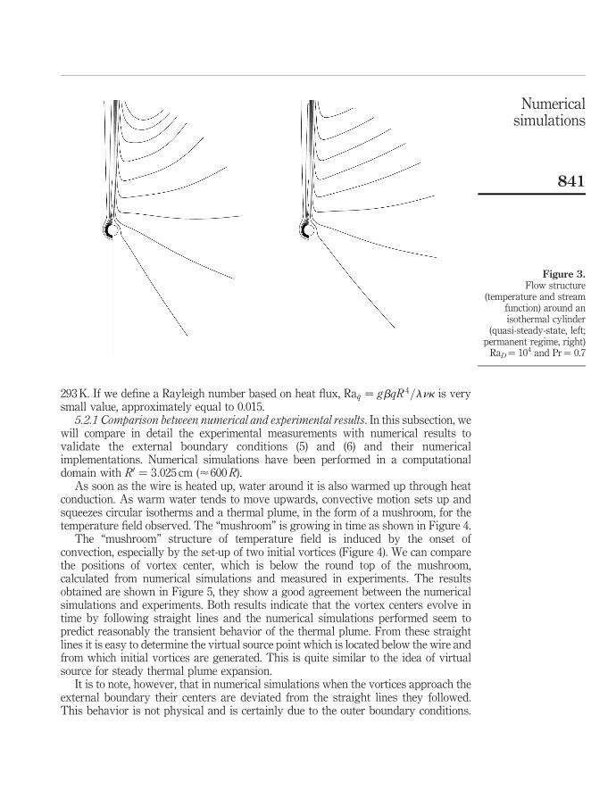
Starting from motionless flow condition and after the transient, time evolution of Nuindicates that a quasi-permanent regime is reached normally and that the proposedouter boundary conditions do not seem to cause any difficulty for numerical procedureto converge. Flow structure corresponding to the quasi-steady-state indicated by Nu isshown in Figure 3. One distinguishes the lower part of thermal plume and outside thethermal plume the incoming flow is downwards, which is somewhat strange and is notconsistent with the flow structure given in Saitoh et al. (1993) by using a very largecomputational domain. However, the value of Nu is equal to 4.791, which agrees wellwith 4.826 in Saitoh et al. (1993). We kept integrating the quasi-permanent solution andobtained steady-state solution which is also shown in Figure 3. Outside the thermalplume the incoming flow is more horizontal but always downwards. Although flowstructure evolved slightly, Nu which decreased only to 4.784 remained almost constant.This suggests that temperature field is insensitive to flow structure outside the thermalplume and that using only Nusselt number is not enough to validate flow structureoutside the thermal plume.
In order to assess the validity of the predicted flow structure, i.e. to know where thepredicted flow is reasonable and where it is not, more detailed results of velocity fieldsare needed; for example, velocity profiles at fixed x and y positions.
5.2 Transient natural convection around a line-sourceIn the experiment, a line-source is represented by a platinum wire of 50mm radiusheated by Joule effect. The heating power is Qv ¼ 3:8 £ 109 W=m3 (which is equivalentto a surface heat flux of q ¼ 9:5 £ 104 W=m2Þ and the room temperature, T0, is equal to
HFF14,7
840
293 K. If we define a Rayleigh number based on heat flux, Raq ¼ gbqR 4=lnk is verysmall value, approximately equal to 0.015.
5.2.1 Comparison between numerical and experimental results. In this subsection, wewill compare in detail the experimental measurements with numerical results tovalidate the external boundary conditions (5) and (6) and their numericalimplementations. Numerical simulations have been performed in a computationaldomain with R0 ¼ 3:025 cm (<600 R).
As soon as the wire is heated up, water around it is also warmed up through heatconduction. As warm water tends to move upwards, convective motion sets up andsqueezes circular isotherms and a thermal plume, in the form of a mushroom, for thetemperature field observed. The “mushroom” is growing in time as shown in Figure 4.
The “mushroom” structure of temperature field is induced by the onset ofconvection, especially by the set-up of two initial vortices (Figure 4). We can comparethe positions of vortex center, which is below the round top of the mushroom,calculated from numerical simulations and measured in experiments. The resultsobtained are shown in Figure 5, they show a good agreement between the numericalsimulations and experiments. Both results indicate that the vortex centers evolve intime by following straight lines and the numerical simulations performed seem topredict reasonably the transient behavior of the thermal plume. From these straightlines it is easy to determine the virtual source point which is located below the wire andfrom which initial vortices are generated. This is quite similar to the idea of virtualsource for steady thermal plume expansion.
It is to note, however, that in numerical simulations when the vortices approach theexternal boundary their centers are deviated from the straight lines they followed.This behavior is not physical and is certainly due to the outer boundary conditions.
Figure 3.Flow structure
(temperature and streamfunction) around anisothermal cylinder
(quasi-steady-state, left;permanent regime, right)
RaD¼ 104 and Pr¼ 0.7
Numericalsimulations
841

Therefore, the outer boundary conditions used cannot predict correctly the fulltransient process, at least not in the entire computational domain. The importantquestion to be answered is whether, in the long-run, the boundary conditions proposedyield reasonable prediction of flow structure. For this purpose, velocity profiles att ¼ 16 s are chosen (i.e. the initial vortices are crossing the outer boundary) andFigure 6 shows the numerical and experimental results at y ¼ 0:5 and 2.5 cm (y is theheight above the wire). Excellent agreement between the experiment and numericalsimulation is observed at y ¼ 0:5 cm: Owing to the fact that the trajectories of theinitial vortices are artificially modified by the outer boundary conditions, at y ¼ 2:5 cmthe discrepancy between the results is important for the horizontal velocity componentwhile agreement remains good for the vertical velocity component. Although the outerboundary conditions used influence the trajectories of the initial vortices, long timeflow structure of the thermal plume is correctly predicted by the numerical methods
Figure 4.Instantaneous velocity(PIV measurements, left)and temperature(numerical results, right)fields in the same spatialscale at t ¼ 6 s (top) and16 s (bottom)
HFF14,7
842

associated with the outer boundary conditions (5) and (6) implemented in the form ofequations (12) and (14).
The transient process can be illustrated by time evolution of temperature field. Thetemperature at y ¼ 0:67 cm above the wire is measured experimentally by athermocouple of 12.7mm diameter and also calculated numerically (Figure 7). Oneobserves again an excellent agreement between the numerical and experimental results.It takes about 4 s for the mushroom of the thermal plume to grow up to y ¼ 0:67 cm; thehead of the mushroom which is hotter than the surrounding water passes this position in2 s ð4 s , t , 6 sÞ and then temperature evolves slowly in time to a constant value.
In comparison with the experimental measurements and with regard to the goodagreement observed, we conclude that the outer boundary conditions used arevalidated. Note, however, that the experimental configuration investigatedcorresponds to a case of very small Rayleigh number (<0.015) and that furtherinvestigation, both numerical and experimental, is needed to validate the outerboundary conditions (5) and (6) at higher Rayleigh numbers.
Figure 6.Velocity profiles (vertical
component on top andhorizontal at bottom) at
t ¼ 16 s and y ¼ 0.5 (left)and 2.5 cm (right)
Figure 5.Measured and computed
positions of initial vortexcenter. Simulations have
been conducted withR 0 ¼ 3.025 cm
Numericalsimulations
843
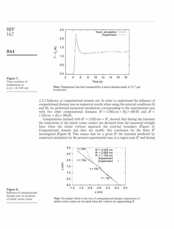
5.2.2 Influence of computational domain size. In order to understand the influence ofcomputational domain size on numerical results when using the external conditions (5)and (6), we performed numerical simulations corresponding to the experimental casewith two other computational domains: R0 ¼ 2:065 cm ¼ R0
2ð<400 RÞ and R0 ¼1:105 cm ¼ R0
3ð<200 RÞ:Computations realized with R0 ¼ 3:025 cm ¼ R 0
1 showed that during the transientthe trajectories of the initial vortex centers are deviated from the measured straightlines when the initial vortices approach the external boundary (Figure 5).Computational domain size does not modify this conclusion for the three R 0
investigated (Figure 8). This means that for a given R 0 the transient predicted bynumerical simulation for the present experimental case, in a region near R 0 and during
Figure 8.Influence of computationaldomain size on positionsof initial vortex center
Figure 7.Time evolution oftemperature at(x, y) ¼ (0, 0.67 cm)
HFF14,7
844

the period when the initial vortices approach the external boundary, will be differentfrom that really taking place in an unbounded domain.
To better illustrate the effect of the outer boundary conditions, velocity andtemperature profiles at t ¼ 6 s and at several positions are shown in Figure 9. Timet ¼ 6 s is the moment when the “mushroom” top is reaching R0
3 and the initial vorticesare crossing this external boundary (Figure 8). The whole set of graphs shown inFigure 9(a) shows that, at this time, results obtained with R0
1 and R02 agree well
independently of the positions, while numerical simulation performed with R03 yields
slightly different results. In the last case, the thermal plume in the form of a mushroomgrows faster than it should. This is why at t ¼ 6 s the position of the mushroom topobtained with R0
3 is above those predicted by the other two simulations (Figure 9(b)).Consequently, at y ¼ 1 cm the values of temperature and vertical velocity componentcalculated with R0
3 are much larger. To some extent the outer boundary conditions (5)
Figure 9.Profiles of vertical velocityand temperature at t ¼ 6 s
Numericalsimulations
845

and (6) make the transient process faster in the region near R0 during the period whenthe mushroom head and the initial vortices cross R0. Nevertheless, it is still safe to saythat at t ¼ 6 s numerical results obtained with R0
3 remain reasonable in the region nearthe heating wire, i.e. r , 0:5 cm ð<100RÞ; because a good agreement between thenumerical results is observed in this region (Figure 9(b)).
Figure 7 also shows that, after the mushroom head travels downstream to a givenposition, flow field reaches a nearly constant value at this position. It is, thus,interesting to know if the outer boundary conditions influence these constant values ormore generally long-time behavior of the flow structure. For this purpose, in Figure 10we will show different profiles of vertical velocity and temperature obtained at t ¼20 s: The surprising fact is that no matter which R0 used there is always in goodagreement with the numerical results. Therefore, for the case investigated thelong-time behavior of flow field is correctly predicted by numerical simulations even
Figure 10.Profiles of vertical velocityand temperature att ¼ 20 s
HFF14,7
846
when one uses a computational domain with R03 (about 200 times the wire radius). This
indicates that the outer boundary conditions (5) and (6) do produce, at least for theexperimental case studied, physically meaningful flow structure at long time. Note thatlong time means long time after the initial vortices exit the computational domain. Itdepends, therefore, on the size of the computational domain. Long time for smallercomputational domains will not be that for larger ones.
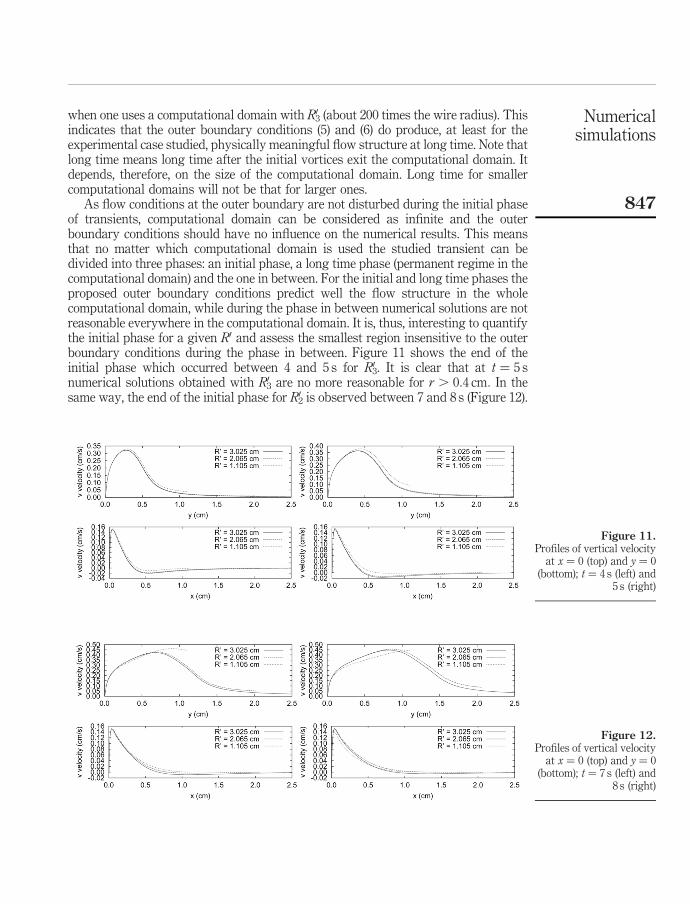
As flow conditions at the outer boundary are not disturbed during the initial phaseof transients, computational domain can be considered as infinite and the outerboundary conditions should have no influence on the numerical results. This meansthat no matter which computational domain is used the studied transient can bedivided into three phases: an initial phase, a long time phase (permanent regime in thecomputational domain) and the one in between. For the initial and long time phases theproposed outer boundary conditions predict well the flow structure in the wholecomputational domain, while during the phase in between numerical solutions are notreasonable everywhere in the computational domain. It is, thus, interesting to quantifythe initial phase for a given R0 and assess the smallest region insensitive to the outerboundary conditions during the phase in between. Figure 11 shows the end of theinitial phase which occurred between 4 and 5 s for R0
3. It is clear that at t ¼ 5 snumerical solutions obtained with R0
3 are no more reasonable for r . 0:4 cm: In thesame way, the end of the initial phase for R0
2 is observed between 7 and 8 s (Figure 12).
Figure 11.Profiles of vertical velocity
at x ¼ 0 (top) and y ¼ 0(bottom); t ¼ 4 s (left) and
5 s (right)
Figure 12.Profiles of vertical velocity
at x ¼ 0 (top) and y ¼ 0(bottom); t ¼ 7 s (left) and
8 s (right)
Numericalsimulations
847

Scaling of the positions of maximum vertical velocity at x ¼ 0 (above the wire) yieldedan empirical law of 0.35R0 as the end of the initial phase, i.e. as far as the position of themaximum vertical velocity above the wire at x ¼ 0 does not exceed 0.35R0 thenumerical solutions are likely to be reasonable everywhere in the computationaldomain. Figure 12 shows also that during the phase in between the smallest regioninsensitive to the boundary conditions for R0
3 is inside the position of maximum verticalvelocity at y ¼ 0 (at the wire level), this also holds for R0
2: Any tolerance of predictionerror will enlarge the smallest region insensitive to the boundary conditions.
The three computational domains used possess a common region which is r # R03:
It is interesting to use the three sets of solutions obtained in r # R03 in order to obtain
extrapolated solutions which would be independent of domain size. Figure 13 showsthe extrapolated solutions given by using quadratic extrapolation in the commonregion at t ¼ 6 and 20 s. As for R0
1, t ¼ 6 s is in the initial phase and solution obtainedwith R0
1 is a good prediction of what should happen in an infinite domain, solutionshave been extrapolated to R0 ¼ 800 R:Att ¼ 20 s; quadratic extrapolation has beendone to R0 ¼ 1; 000 R: At t ¼ 6 s; thermal plume of mushroom structure is approachingthe outer boundary at R0
3 and part of initial vortices is out of the computational domain.It is another form of flow fields shown in Figure 4. At t ¼ 20 s inside R0
3; only the lowerpart of the thermal plume is observed and fluid motion is mainly upwards. This is inqualitative agreement with flow structures shown in Linan and Kurdyomov (1998) forsmall Grashof numbers.
6. Concluding remarksIn order to pave the way for numerical simulations of external natural convectionand the corresponding transients, we implemented, for solving the Navier-Stokesequations under Boussinesq assumption in velocity-pressure formulation, a
Figure 13.Extrapolated solutions(temperature and streamfunction) in R 0
3 at t¼ 6 s(left) and 20 s (right)around a line-source
HFF14,7
848
numerical code using spectral methods, domain decomposition technique withSchur complement, projection method (velocity-pressure coupling) and new outerboundary conditions.
The validation of the code implemented was done through performing experimentalmeasurements. A thin platinum wire heated by Joule effect has been used in theexperiment to represent a line-source and Rayleigh number investigated, Raq, is about0.015. During the transient, time evolution of pointwise temperature is measured bymicro-thermocouples and velocity field by PIV. Numerical results agree well with theexperimental data and the code implemented (numerical methods and outer boundaryconditions used) was thus validated.
Numerical simulations were also realized for the experimental case in order toreveal the influence of computational domain size on numerical results. It is shownthat the proposed boundary conditions (5) and (6) make transient process faster thanit should be when the initial vortices approach the external boundary. It is also shownthat the numerical results obtained at long time in the experimental case predict wellthe flow structure in the whole computational domain. No matter whichcomputational domain size R0 is, the transient of the experimental case, yielded bynumerical simulations using the proposed outer boundary conditions, can be dividedinto three phases: the initial phase, the long time phase and the one in between.During the initial and long time phases, numerical results are reasonable everywherein the computational domain. The end of the initial phase is defined by the time whenthe vertical position of maximal vertical velocity above the wire at x ¼ 0 exceeds0.35R0 and the long time phase means long time after the initial vortices exit thecomputational domain. During the phase in between, the present numerical resultsare not reasonable everywhere: the smallest region which is insensitive to the outerboundary conditions is inside the position of maximum vertical velocity at y ¼ 0:This region can be enlarged provided some tolerance of prediction error. If predictionerror can be accepted to some extent, numerical simulation of transient externalnatural convection using the proposed outer boundary conditions is feasible becausenumerical results obtained are reasonable at least in a region near the line-sourceduring the entire transient.
It is important to point out that Rayleigh number of the testing case is small, theproposed boundary conditions (5) and (6) are at least appropriate for low Rayleighnumber cases. Further studies, both experimental and numerical, should be done tovalidate these conditions at higher Rayleigh numbers. Nevertheless, in order to showthat the proposed outer boundary conditions work also at high Rayleigh number,numerical simulations have been done for an isothermal cylinder at RaD ¼ 104 andPr ¼ 0:7 and the average Nusselt number along the cylinder surface obtained agreeswell with the results in the literature.
As the position of the outer boundary is chosen to enable numerical simulation ofexternal natural convection and the flow conditions on such a boundary are unknown,one cannot expect that numerical simulations undertaken in this way predicts well thecorresponding flow structure everywhere in the whole computational domain.Numerical prediction has, however, to be reasonable and even good in part of thecomputational domain near the heating element. This is observed from the numericalsimulations we performed and should be the rule of validating numerical simulations ofexternal natural convection.
Numericalsimulations
849

References
Bernard, C. and Maday, Y. (1992), “Approximations spectrales de problemes aux limiteselliptiques”, Collection Mathematiques & Applications, Springer Verlag, Berlin.
Canuto, C., Hussaini, M., Quarteroni, A. and Zang, T. (1988), Spectral Methods in Fluid Dynamics,Springer Verlag, Berlin.
Duluc, M-C., Xin, S. and Le Quere, P. (2003), “Transient natural convection and conjugatetransients around a line heat source”, Int. J. Heat Mass Trans., Vol. 46, pp. 341-54.
Farouk, B. and Guceri, S. (1981), “Natural convection from a horizontal cylinder – laminarregime”, J. Heat Transfer, Vol. 103, pp. 522-7.
Fujii, T., Morioka, I. and Uehara, H. (1973), “Buoyant plume above a horizontal line heat source”,Int. J. Heat Mass Trans., Vol. 16, pp. 755-68.
Funaro, D., Quarteroni, A. and Zanolli, P. (1988), “An iterative procedure with interface relaxationfor domain decomposition methods”, SIAM J. Numer. Anal., Vol. 25 No. 6, pp. 1213-36.
Guermond, J-L. and Quartapelle, L. (1998), “On the approximation of the unsteady Navier-Stokesequations by finite element projection methods”, Numer. Math., Vol. 80 No. 5, pp. 207-38.
Karageorghis, A. and Paprzycki, M. (1999), “Conditioning of pseudospectral matrices for certaindomain decomposition”, J. Sci. Comp., Vol. 14 No. 1, pp. 107-19.
Kelkar, K. and Choudhury, D. (2000), “Numerical method for the prediction of incompressibleflow and heat transfer in domains with specified pressure boundary conditions”, Numer.Heat Transf. B, Vol. 38, pp. 15-36.
Kuehn, T. and Goldstein, R. (1980), “Numerical solutions to the Navier-Stokes equations forlaminar natural convection about a horizontal isothermal circular cylinder”, Int. J. HeatMass Trans., Vol. 23, pp. 971-9.
Linan, A. and Kurdyomov, V. (1998), “Laminar free convection induced by a line heat source andheat transfer from wires at small Grashof numbers”, J. Fluid Mech., Vol. 362, pp. 199-227.
Louchart, O., Randriamampianina, A. and Leonardi, E. (1998), “Spectral domain decompositiontechnique for the incompressible Navier-Stokes equations”, Numer. Heat Transf. A,Vol. 34, pp. 495-518.
Ostroumov, G. (1956), “Unsteady heat convection near a horizontal cylinder”, Sov. Phys. Tech.Phys., Vol. 1 No. 12, pp. 2627-41.
Quenot, C., Pakleza, J. and Kowalewski, T. (1998), “Particle image velocimetry with optical flow”,Exp. Fluids, Vol. 25, pp. 177-89.
Saitoh, T., Sajiki, T. and Maruhara, K. (1993), “Benchmark solutions to natural convection heattransfer problem around a horizontal cylinder”, Int. J. Heat Mass Trans., Vol. 36,pp. 1251-9.
Schorr, A.W. and Gebhart, B. (1970), “An experimental investigation of natural convection wakesabove a line heat source”, Int. J. Heat Mass Trans., Vol. 13, pp. 557-71.
Smith, B., Bjorstad, P. and Cropp, W. (1996), Domain Decomposition: Parallel Multilevel Methodsfor Elliptic Partial Differential Equations, Cambridge University Press, New York, NY.
Wang, P., Kahawita, R. and Nguyen, T. (1990), “Numerical computation of the natural convectionflow about a horizontal cylinder using splines”, Numer. Heat Transf. A, Vol. 17, pp. 191-215.
Yosinobu, H., Onishi, Y., Enyo, S. and Wakitani, S. (1979), “Experimental study on instability of anatural convection flow above a horizontal line heat source”, J. Phys. Soc. Jpn, Vol. 47 No. 1,pp. 161-71.
Zanolli, P. (1987), “Domain decomposition algorithms for spectral methods”, Calcolo, Vol. 24,pp. 202-40.
HFF14,7
850