Numerical Schemes for Hyperbolic Balance Laws â€“ Applications to

1. Introduction

Balance laws arise from many areas of engineering practice specifically from the fluidmechanics. Many numerical methods for the solution of these balanced laws weredeveloped in recent decades. The numerical methods are based on two views: solvinghyperbolic PDE with a nonzero source term (the obvious description of the central andcentral-upwind schemes; (Kurganov & Levy, 2002; LeVeque, 2004)) or solving the augmentedquasilinear nonconservative formulation (Gosse, 2001; Le Floch & Tzavaras, 1999; Pares, 2006).Furthermore, the methods can be interpreted using flux-difference splitting (or flux-vectorsplitting), or by selecting adaptive intervals and the transformation to the semidiscreteform (for example (Kurganov & Petrova, 2000)). We prefer the augmented quasilinearnonconservative formulation solved by the flux-difference splitting in our text. We try toformulate the methods in the most general form. The range of this text does not give thecomplete overview of currently used methods.

2. Mathematical models

In this section we describe the specific mathematical models based on hyperbolic balancedlaws. There are many models that describe fluid flow phenomena but we are interested in thetwo type of them: models described open channel flow and urethra flow.

2.1 Shallow water equations

We are interested in solving the problem related to the fluid flow through the channel with thegeneral cross-section area described by

at + qx = 0, (1)

qt +

(q2

a+ gI1

)

x

= −gabx + gI2,

where a = a(x, t) is the unknown cross-section area, q = q(x, t) is the unknown discharge,b = b(x) is given function of elevation of the bottom, g is the gravitational constant and

I1 =∫ h(x,t)

0[h(x, t)− η]σ(x, η)dη, (2)

Numerical Schemes for Hyperbolic Balance Laws – Applications to Fluid Flow Problems

Marek Brandner, Ji í Egermaier and Hana Kopincová The University of West Bohemia

Czech Republic

2

www.intechopen.com

2 Will-be-set-by-IN-TECH

I2 =∫ h(x,t)

0(h(x, t)− η)

[∂σ(x, η)

∂x

]

dη, (3)

here η is the depth integration variable, h(x, t) is the water depth and σ(x, η) is the width ofthe cross-section at the depth η. The derivation can be found in e.g. (Cunge at al., 1980).

The first special case are the equations reflecting the fluid flow through the spatially varyingrectangular channel

at + qx = 0, (4)

qt +

(q2

a+

ga2

2l

)

x

=ga2

2l2lx − gabx,

with l = l(x) being the function describing the width of the channel, and second one thesystem for the constant rectangular channel

ht + (hu)x = 0, (5)

(hu)t +

(

hu2 +1

2gh2

)

x

= −ghbx.

In the above equation, h(x, t) is the water depth and u(x, t) is the horizontal velocity. It alsopossible to add some friction term to the system described above. For example, we can write

ht + (hv)x = 0,

(hv)t +

(

hv2 +1

2gh2

)

x

= −ghBx − gM2 hv|hv|

h7/3, (6)

where M is Manning’s coefficient.

All of the presented systems can be written in the compact matrix form

qt + [f(q, x)]x = ψ(q, x), (7)

with q(x, t) being the vector of conserved quantities, f(q, x) the flux function and ψ(q, x) thesource term. This relation represents the balance laws.

It is possible to use any augmented formulation, which is suitable for rewriting the system tothe quasilinear homogeneous one. For example, we can obtain

ht + (hu)x = 0, (8)

(hu)t +

(

hu2 +1

2gh2

)

x

= −ghbx,

bt = 0,

i.e. ⎡

⎣

hhvb

⎤

⎦

t

+

⎡

⎣

0 1 0−v2 + gh 2v −gh

0 0 0

⎤

⎦

⎡

⎣

hhvb

⎤

⎦

x

=

⎡

⎣

000

⎤

⎦ . (9)

36 Finite Volume Method – Powerful Means of Engineering Design

www.intechopen.com

Numerical Schemes for Hyperbolic Balance Laws. Applications to Fluid Flow Problems 3

2.2 Urethra flow

We now briefly introduce a problem describing fluid flow through the elastic tube representedby hyperbolic partial differential equations with the source term. In the case of the maleurethra, the system based on model in (Stergiopulos at al., 1993) has the following form

at + qx = 0,

qt +(

q2

a + a2

2ρβ

)

x= a

ρ

(a0β

)

x+ a2

2ρβ2 βx −q2

4a2

√πa λ(Re),

(10)

where a = a(x, t) is the unknown cross-section area, q = q(x, t) is the unknown flow rate(we also denote v = v(x, t) as the fluid velocity, v =

qa ), ρ is the fluid density, a0 = a0(x) is

the cross-section of the tube under no pressure, β = β(x, t) is the coefficient describing tubecompliance and λ(Re) is the Mooney-Darcy friction factor (λ(Re) = 64/Re for laminar flow).Re is the Reynolds number defined by

Re =ρq

μa

√

4a

π, (11)

where μ is fluid viscosity. This model contains constitutive relation between the pressure andthe cross section of the tube

p =a − a0

β+ pe, (12)

where pe is surrounding pressure.

3. Conservative and nonconservative problems and numerical schemes

3.1 Conservative problems and numerical schemes

We consider the conservation law in the conservative form

qt + [f(q)]x = 0, x ∈ R, t ∈ (0, T), (13)

q(x, 0) = q0(x), x ∈ R,

The numerical scheme based on finite volume discretization in the conservation form can bewritten as follows,

Qn+1j = Qn

j −Δt

Δx(Fn

j+1/2 − Fnj−1/2). (14)

We use also the semidiscrete version of (14)

∂Qj

∂t= −

1

Δx(Fj+1/2 − Fj−1/2). (15)

The relation (14) can be derived as the approximation of the integral conservation law at the

interval⟨

xj−1/2, xj+1/2

⟩

from time level tn to tn+1

1Δx

xj+1/2∫

xj−1/2

q(x, tn+1)dx = 1Δx

xj+1/2∫

xj−1/2

q(x, tn)dx−

− 1Δt

[tn+1∫

tn

f(q(xj+1/2, t))dt −tn+1∫

tn

f(q(xj−1/2, t))dt

]

.

(16)

37Numerical Schemes for Hyperbolic Balance Laws – Applications to Fluid Flow Problems

www.intechopen.com


The previous relations lead to the following approximations of integral averages

Qnj ≈

1

Δx

∫ xj+1/2

xj−1/2

q(x, tn)dx,

Fnj+1/2 ≈

1

Δt

∫ tn+1

tn

f(q(xj+1/2, t))dt. (17)

Numerical fluxes Fnj+1/2 are usually defined by the approximate solution of the Riemann

problem between states Qnj+1 and Qn

j (this technique is called the flux difference splitting;

it will be described in the following parts) or by the Boltzmann approach (flux vectorsplitting; it will be described later). In what follows, we use the notation Q+

j+1/2 and

Q−j+1/2 for the reconstructed values of unknown function. Reconstructed values represent

the approximations of limit values at the points xj+1/2. The most common reconstructionsare based on the minmod function (see for example (Kurganov & Tadmor, 2000)) or ENO andWENO techniques (Crnjaric-Zic at al., 2004).

If the exact solution of the problem has a compact support in the interval 〈0, T〉 then it ispossible to show, that the scheme (15) is conservative, i.e.

∞

∑j=−∞

Qn+1j =

∞

∑j=−∞

Qnj . (18)

The uniqueness of discontinuous solutions to the conservation laws is not guaranteed.Therefore the additional conditions, based on physical considerations, are required to isolatethe physically relevant solution. The most common condition is called entropy condition. Theunique entropy satisfying weak solution q holds

[η(q)]t + [ϕ(q)]x ≤ 0, (19)

for the convex entropy functions η(q) and corresponding entropy fluxes ϕ(q) (for example see(LeVeque, 2004)).

If the conservation law (13) is solved by the consistent method in conservation form (15) theLax-Wendroff theorem is valid (LeVeque, 2004): if the approximate function Q(x, t) convergedto the function q(x, t) for the Δx, Δt → 0, the function q(x, t) is the weak solution of the problem(13).

Many theoretical results in the field of hyperbolic PDEs can be found in the literature. Forexample, for scalar problems with the convex flux function, the convergence of the somemethod to the entropy-satisfying weak solutions, is proven. It means that if the solution qǫ ofthe problem

qt + [ f (q)]x = ǫqxx, x ∈ R, 0 < t < T, ǫ > 0,q(x, 0) = q0(x), x ∈ R.

(20)

exists and the limit q∗ = limǫ→0+

qǫ exists too than q∗ is the entropy-satisfying weak solutions of

the problem (20).

It is possible to define the appropriate properties of the methods. For example, in the caseof scalar problem, TVD (Total Variation Diminishing) property, which ensures that the total


www.intechopen.com


variation of the solution is non-increasing, i.e.

∞

∑j=−∞

|Qn+1j+1 − Qn+1

j | ≤∞

∑j=−∞

|Qnj+1 − Qn

j | (21)

for all time layers tn. This property is important for limitation of the oscillations in the solution.

3.2 Nonconservative problems

We consider the nonlinear hyperbolic problem in nonconservative form

qt + A(q)qx = 0, x ∈ R, t ∈ (0, T), (22)

q(x, 0) = q0(x), x ∈ R.

The numerical schemes for solving problems (22) can be written in fluctuation form

∂Qj

∂t= −

1

Δx[A−(Q−

j+1/2, Q+j+1/2) + A(Q−

j+1/2, Q+j−1/2) + A+(Q−

j−1/2, Q+j−1/2)], (23)

where A±(Q−j+1/2, Q+

j+1/2) are so called fluctuations. They can be defined by the sum of waves

moving to the right or to the left. The directions are dependent on the signs of the speeds ofthese waves, which are related to the eigenvalues of matrix A(q).

When the problem (22) is derived from the conservation form (13), i.e. f′(q) = A(q) is theJacobi matrix of the system, fluctuations can be defined as follows

A(Q−j+1/2, Q+

j−1/2) = f(Q−j+1/2)− f(Q+

j−1/2),

A−(Q−j+1/2, Q+

j+1/2) = F−j+1/2 − f(Q−

j+1/2),

A+(Q−j−1/2, Q+

j−1/2) = f(Q+j−1/2)− F+

j−1/2.

(24)

4. Riemann problem

4.1 Riemann problem for conservative systems

The Riemann problem is the special problem based on finite volume discretization with thediscontinuous initial condition. In the nonlinear case it has the form

qt + [f(q)]x = 0, x ∈ R, t ∈ (0, T),

q(x, 0) =

{

Qnj , x < xj+1/2,

Qnj+1, x > xj+1/2.

(25)

We solve the transitions between two states, but this solution could not exists in general. Thesetransitions can be rarefaction waves, shock waves or contact discontinuities. Rarefaction waveis case of a continuous solution when the following equality holds

q(x, t) = q(ξ(x, t)), (26)

whereq′(ξ) = α(ξ)rp(ξ) (27)


www.intechopen.com


for any function ξ(x, t), where α(ξ) is a coefficient dependent on the function ξ and Rp(ξ) isthe corresponding p-th eigenvector of the Jacobi matrix f′(u).

Shock waves and contact discontinuities are special cases of discontinuous solutions. Therequirement that this solution should be (see (LeVeque, 2004)) a weak solution of the problem(25) leads to the following relation

s(q+ − q−) = f(q+)− f(q−), (28)

where s is the speed of the propagation of the discontinuities. The relation (28) is known asthe Rankine-Hugoniot jump condition. In some cases it is possible to construct the solution ofRiemann problem as the sequence of the transitions between the discontinuous states (in thecase of strong nonlinearity the discontinuous solution consists of the shock waves, in the caseof linear degeneration solution consists of the contact discontinuities).

In the case of a linear problem f(q) = Aq it is known that the initial state of each characteristicvariable wp is moving at a speed that corresponds to the eigenvalue λp of the matrix A.The solution is a system of constant states separated by discontinuities that move at speedscorrespondent to eigenvalues. Therefore, the jump Qj+1 − Qj over p-th discontinuity can beexpressed as,

(wpj+1 − w

pj )r

p = αprp, (29)

where rp is the p-th eigenvector of matrix A. The relation (29) represents the initial jump inthe characteristic variable wp and at the same time q = Rw. Therefore, the solution of linearRiemann problem can be defined by the decomposition of the initial jump of the unknownfunction to the eigenvectors rp of the Jacobi matrix A = f′(q)

Qj+1 − Qj =m

∑p=1

αprp. (30)

The discontinuities Wp = αprp are called waves and they are propagated by the speeds λp.For details see (LeVeque, 2004).

4.2 Riemann problem for nonconservative systems

In this section we are interested in nonlinear systems in nonconservative form

qt + A(q)qx = 0, x ∈ R, t > 0, (31)

q0 ∈ [BV(R)]m,

where q ∈ Rm, q → A(q) is smooth locally bounded matrix-valued map, matrix A(q)

is strictly hyperbolic (diagonalizable, with real and different eigenvalues). We suppose thatA(q) is not Jacobi matrix so it is not possible to rewrite nonconservative system in conservativeform (13). Here, BV[(R)]m is function space contains functions with bounded total variation.

Above mentioned system makes sense only if q is differentiable. In the case when q admitsdiscontinuities at a point, A(q) may admits discontinuities as well and qx contains deltafunction with singularity at this point. Then A(q)qx is product of Heaviside function withdelta function and in general is not unique. There is possibility to smooth out” of this functionover width ǫ, for example by adding viscosity or diffusion. Then we get well defined product


www.intechopen.com


of continuous functions. The limiting behavior for ǫ → 0 is strongly depend on “smoothingout.”

Under a special assumption, the nonconservative product A(q)qx can be understood as aBorel measure. In the following we introduce basic theorems and definitions, for details see(Gosse, 2001; Le Floch, 1989; Le Floch & Tzavaras, 1999; Pares, 2006).

Definition 4.1. A path φ in Ω ∈ Rm is a family of smooth maps 〈0, 1〉 × Ω × Ω → Ω satisfying:

• φ(0; ql , qr) = ql and φ(1; ql , qr) = qr, ∀ql , qr ∈ Ω, ∀s ∈ 〈0, 1〉,

• for each bounded set O ∈ Ω, there exists a constant k > 0 such that

∣∣∣∣

∂φ

∂s(s; ql , qr)

∣∣∣∣≤ k |qr − ql |

for any ql , qr ∈ O and almost all s ∈ 〈0, 1〉,

• for each bounded set O ∈ Ω, there exists a constant K > 0 such that

∣∣∣∣

∂φ

∂s(s; q1

l , q1r )−

∂φ

∂s(s; q2

l , q2r )

∣∣∣∣≤ K

(∣∣∣q1

l − q2l

∣∣∣+

∣∣∣q1

r − q2r

∣∣∣

)

for any q1l , q1

r , q2l , q2

r ∈ O and almost all s ∈ 〈0, 1〉.

Theorem 4.1 (Dal Maso, Le Floch, Murat). Let q : (a, b) → Rm be a function with bounded

variation and A : Rm → R

m×m a locally bounded function. There exists a unique signed Borelmeasure μ on (a, b) characterized by following properties:

1. if x → q(x) is continuous on an open set o ∈ (a, b) then

μ(o) =∫

o

A(q)∂q

∂xdx,

2. if x0 ∈ (a, b) is a discontinuity point of x → q(x), then

μ(x0) =

1∫

0

A(φ(s; q(x−0 ), q(x+0 ))

) ∂φ

∂s(s; q(x−0 ), q(x+0 )) ds,

where we denote q(x−0 ) = limx→x−

0

q(x) and q(x+0 ) = limx→x+

0

q(x).

Remark 4.1. Borel measure μ is called nonconservative product and is usually written [A(q)qx]φ.

Remark 4.2. In the case where A(q) = f′(q) then Borel measure, [A(q)qx]φ = f(q)x is independentof the path φ.

Definition 4.2 (Weak solution). Let φ be a family of paths in the sense of definition 4.1. A functionq ∈ [L∞(R×R

+) ∩BVloc(R×R+)]m is a weak solution of system (31), if it satisfies

qt + [A(q)qx]φ = 0, (32)

as a bounded Borel measure on R×R+.


www.intechopen.com


Definition 4.3 (Entropy solution). Given an entropy pair (η, ϕ)(entropy, entropy flux) for (31), i.e.a pair of regular functions Ω → R, such that

∇ϕ(q) = ∇η(q) · A(q), ∀q ∈ Ω. (33)

A weak solution is said to be entropic if it satisfies the inequality

∂η(q)

∂t+

∂ϕ(q)

∂x≤ 0 (34)

in the sense of distribution.

Function q(x, t) is weak solution if and only if, across a discontinuity with speed ζ, it satisfiesgeneralized Rankine-Hugoniot condition,

− ζ(qr − ql) +

1∫

0

A (φ(s; ql , qr))∂φ

∂s(s; ql , qr) ds = 0. (35)

Now we define the Riemann problem for nonconservative strictly hyperbolic system:

qt + A(q)qx = 0, x ∈ R, t > 0 (36)

with an initial condition

q(x, 0) = q0(x) =

{ql pro x < 0,

qr pro x > 0,(37)

where ql , qr ∈ Rm are vectors of constants.

Theorem 4.2. Let φ be a family of path in the sense of definition 4.1. Assume that system (36) isstrictly hyperbolic with genuinely nonlinear or linearly degenerate characteristic field and the family ofpath φ satisfies

∂φ

∂q1(1; q0, q0)−

∂φ

∂q1(0; q0, q0) = I, ∀q0 ∈ R

m. (38)

Then, for |qr − ql | small enough, the Riemann problem (36) and (37) has a solution q(x, t) withbounded variation, which depends only on x

t and has Lax’s structure. That is q(x, t) consist of m + 1constant states separated by shock waves, rarefaction waves or contact discontinuities.

The solution of the Riemann problem for nonconservative system is related to the solutionof the Riemann problem for conservative system. The only difference is in the case of shockwave, precisely in Rankine-Hugoniot condition formulation.

Before we define a class of useful numerical methods, we introduce a brief motivation, whichcan be in details found in (Gosse, 2001). Suppose nonconservative system

qt + A(q)qx = 0, x ∈ R, t > 0 (39)


www.intechopen.com


and suppose family of path in the sense of definition 4.1. If q(x, t) is piecewice regular weaksolution then for given time t, the Borel measure can be written in following form

μφ(o) = μφa (o) + μ

φs =

∫

o

A(q)qx dx + ∑k

⎡

⎣

1∫

0

A(φ(s; q−k , q+

k ))∂φ

∂s(s; q−

k , q+k ) ds

⎤

⎦δx=xk(t), (40)

where index k represents number of discontinuities in solution, xk(t) are discontinuity pointsin the time t > 0 and q−

k = limx→xk(t)−

q(x, t), q+k = lim

x→xk(t)+q(x, t), δx=xk(t) is Dirac measure at

the point x = xk(t). Then we can get

Qn+1j = Qn

j −1

Δx

tn+1∫

tn

μφ(Ij) dt. (41)

The amount of the quantity on the cell boundaries xj+1/2 can be splitted into contribution to

cell Ij+1 and the contribution to the cell Ij. In other words, we split it into two terms A±j+1/2.

So the sum of this terms can be understood as a discrete representation of thetn+1∫

tn

μφs dt and

Aj ≈tn+1∫

tn

μφa (Ij)dt. By this way we get generalisation of classical conservative finite volume

methods, see (Pares, 2006), i.e.

Qn+1j = Qn

j −Δt

Δx[A+

j−1/2 + Aj + A−j+1/2]. (42)

Definition 4.4. Given a family of path φ, a numerical scheme is said to be path-conservation if it canbe written in form (42), where

A±j+1/2 = A±(qj−p, . . . , qj+q),

Aj = A(qj−p, . . . , qj+q),

A±, A : Ωp+q+1 → Ω being continuous functions satisfying

1.A±(q, . . . , q) = 0, ∀q ∈ Ω, (43)

2.

A−(q−p, . . . , qq) + A+(q−p, . . . , qq) =1∫

0

A(φ(s; ql , qr))∂φ∂s (s; ql , qr) ds

∀qj ∈ Ω, j = −p, . . . , q.

(44)

3.

A(q, . . . , q) =

xj+1/2∫

xj−1/2

A(q)qx dx. (45)

Remark 4.3. If A(q) = f′(q) then path-conservation scheme is consistent and conservative (thatis if the nonconservative system can be written as conservative one, path-conservative method becomeclassical conservative and consistent). Notice here that A± are fluctuations, see 3.2.


www.intechopen.com


4.3 The properties of exact solution

Consider a system in conservative form with special right hand side (this system agrees withshallow water system (5))

qt + f(q)x = S(q)σx. (46)

This system can be rewritten in a following homogeneous nonconservative form

ut + A(u)ux = 0, (47)

where

u =

[qσ

]

and A(u) =

[∂f∂u (u) −S(u)

0 0

]

,

where ∂f∂u (w) denotes Jacobian matrix of flux f. In order to define weak solutions of the system

(47) we have to choose family of paths (see definition 4.1 and theorem 4.2). And followingrequirement become natural: if u = [q, σ]T is a weak solution of the nonconservative system(47) and σ is constant, then q must be weak solution of the homogeneous system of conservationlaws, i.e. (46) with zero right hand side. By this requirement we impose addition condition offamily of paths:

if ul and ur are such that σl = σr = σ, then

Φ(s; ul , ur) = σ, s ∈ 〈0, 1〉 . (48)

For these systems, there are no difficulties with convergence. Moreover, the shock wavespropagating in regions where σ is continuous are correctly captured independently of thechoice of path. For details see (Le Floch at al., 2008).

5. Approximate Riemann solvers

There are many numerical schemes for solving (7) with different properties and possibilitiesof failing. The main types of the finite volume schemes are the central, upwind andcentral-upwind schemes. All these schemes relate together in variety of ways. We caninterpret them as schemes with different deep knowledge about structure of the solution ofRiemann problem. For example, the same scheme can be interpreted as the HLL solver (anapproximate Riemann solver) or as the central–upwind scheme.

The main requirements on the numerical schemes are the consistency (in the finite volumesense, i.e. consistency with the flux function), the conservativity (if there is possibility torewrite the problem to the conservative form it is required to have conservative numericalscheme), positive semidefiniteness (the scheme preserves nonnegativity of some quantities,which are essentially nonnegative from their physical fundamental) and the well-balancing(the schemes maintain some or all steady states which can occur). The next properties arethe order of the schemes and stability. From the computational point of view there are otherproperties such as robustness, simplicity and computational efficiency. The second and thirdof these properties are typical for the central methods, but they are not common for schemebased on Roe’s solver.

The steady states mean that the unknown quantities do not change in the time, i.e. qt = 0in (7), and the flux function must balance the right hand side, i.e. [f(q)]x = ψ(q, x). Someschemes are constructed to preserve some special steady states for example called “lake atrest” in open channel flow problems, where there is no motion and the free surface is constant.


www.intechopen.com


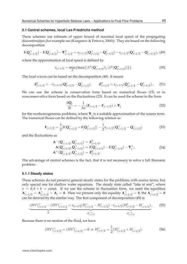
5.1 Central schemes, local Lax-Friedrichs method

These schemes use estimate of upper bound of maximal local speed of the propagatingdiscontinuities (for example see (Kurganov & Petrova, 2000)). They are based on the followingdecomposition

f(Q+j+1/2)− f(Q−

j+1/2)−Ψ±j+1/2 = sj+1/2(Q

+j+1/2 −Q∗

j+1/2)− sj+1/2(Q∗j+1/2 −Q−

j+1/2), (49)

where the approximation of local speed is defined by

sj+1/2 = maxp

{max{|λp(Q−j+1/2)|, |λ

p(Q+j+1/2)|}}. (50)

The local waves can be based on the decomposition (49). It means

Z1j+1/2 = −sj+1/2(Q

∗j+1/2 − Q−

j+1/2), Z2j+1/2 = sj+1/2(Q

+j+1/2 − Q∗

j+1/2). (51)

We can use the scheme in conservation form based on numerical fluxes (15) or innonconservative form based on the fluctuations (23). It can be used the scheme in the form

∂Qj

∂t= −

1

Δx(Fj+1/2 − Fj−1/2) + Ψj (52)

for the nonhomogeneous problems, where Ψj is a suitable approximation of the source term.The numerical fluxes can be defined by the following relation as

Fj+1/2 =1

2[f(Q−

j+1/2 + f(Q+j+1/2)]−

1

2sj+1/2(Q

+j+1/2 − Q−

j+1/2) (53)

and the fluctuations as

A−(Q−j+1/2, Q+

j+1/2) = Z1j+1/2,

A(Q−j+1/2, Q+

j−1/2) = f(Q−j+1/2)− f(Q+

j−1/2)− Ψ∓j ,

A+(Q−j+1/2, Q+

j+1/2) = Z2j+1/2.

(54)

The advantage of central schemes is the fact, that it is not necessary to solve a full Riemannproblem.

5.1.1 Steady states

These schemes do not preserve general steady states for the problems with source terms, butonly special one for shallow water equations. The steady state called “lake at rest”, wherev = 0, h + b = const. If we use the scheme in fluctuation form, we need the equalitiesA−

j+1/2 = A+j+1/2 = Aj = 0. Here we present only the equality A+

j+1/2 = 0, the A−j+1/2 = 0

can be derived by the similar way. The first component of decomposition (49) is

(HV)+j+1/2 − (HV)−j+1/2︸︷︷︸

0

= sj+1/2(H+j+1/2 − H∗

j+1/2)︸︷︷︸

A+,1j+1/2

−sj+1/2(H∗j+1/2 − H−

j+1/2)︸︷︷︸

A−,1j+1/2

. (55)

Because there is no motion of the fluid, we have

(HV)+j+1/2 = (HV)−j+1/2 = 0 ⇒ H∗j+1/2 =

1

2(H+

j+1/2 + H−j+1/2). (56)


www.intechopen.com


Fig. 1. The central methods construct only one middle state.

We consider nonhomogeneous problem, it means, that the bx �= 0. The constant water levelthen includes hx �= 0. Therefore the fluctuation are not equal to zero in general.

H+j+1/2 �= H−

j+1/2 ⇒ H+j+1/2 − H∗

j+1/2 �= 0 ⇒ A+,1j+1/2 �= 0. (57)

This situation is illustrated at the Fig.1. It can be seen that one middle state is in contradictionwith physical model with source terms. This method could preserve only steady states thatthe reconstruction of unknown function is constant. This leads to the following modificationof the system (5). We define new unknown function representing water level y = h + b. Theshallow water equation can be modified to the following form

[y

(y − B)v

]

t

+

[(y − B)v

(y − B)v2 + 12 g(y − B)2

]

x

=

[0

−g(y − B)Bx

]

. (58)

Then the first component of decomposition (49) is

((Y − B)V)+j+1/2 − ((Y − B)V)−j+1/2︸︷︷︸

0

= sj+1/2(Y+j+1/2 − Y∗

j+1/2)︸︷︷︸

A+,1j+1/2

−sj+1/2(Y∗j+1/2 − Y−

j+1/2)︸︷︷︸

A−,1j+1/2

.

(59)Again, no motion of the water ensures

((Y − B)V)+j+1/2 = ((Y − B)V)−j+1/2 = 0 ⇒ Y∗j+1/2 =

1

2(Y+

j+1/2 + Y−j+1/2). (60)

Constant water level means yx = 0 and then

Y+j+1/2 = Y−

j+1/2 ⇒ Y+j+1/2 − Y∗

j+1/2 = 0 ⇒ A+,1j+1/2 = 0. (61)

The second component of decomposition (49) is

f 2(Q+j+1/2)− f 2(Q−

j+1/2)− Ψ2,±j+1/2

︸︷︷︸

0 (for suitable approximation)

=

= sj+1/2(Q+,2j+1/2 − Q∗,2

j+1/2)︸︷︷︸

A+,2j+1/2

−sj+1/2(Q∗,2j+1/2 − Q−,2

j+1/2)︸︷︷︸

A−,2j+1/2

. (62)


www.intechopen.com


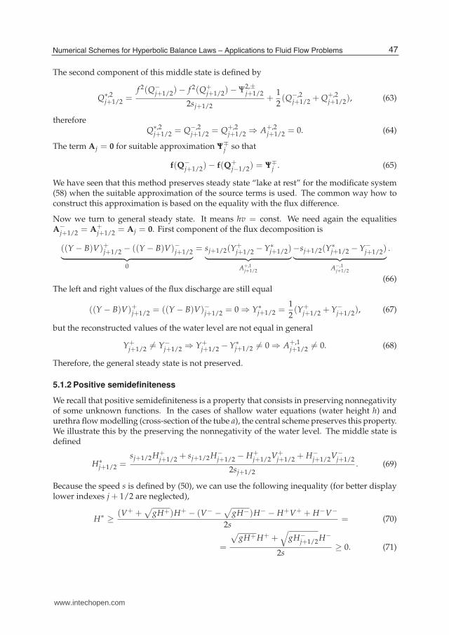
The second component of this middle state is defined by

Q∗,2j+1/2 =

f 2(Q−j+1/2)− f 2(Q+

j+1/2)− Ψ2,±j+1/2

2sj+1/2+

1

2(Q−,2

j+1/2 + Q+,2j+1/2), (63)

thereforeQ∗,2

j+1/2 = Q−,2j+1/2 = Q+,2

j+1/2 ⇒ A+,2j+1/2 = 0. (64)

The term Aj = 0 for suitable approximation Ψ∓j so that

f(Q−j+1/2)− f(Q+

j−1/2) = Ψ∓j . (65)

We have seen that this method preserves steady state “lake at rest” for the modificate system(58) when the suitable approximation of the source terms is used. The common way how toconstruct this approximation is based on the equality with the flux difference.

Now we turn to general steady state. It means hv = const. We need again the equalitiesA−

j+1/2 = A+j+1/2 = Aj = 0. First component of the flux decomposition is

((Y − B)V)+j+1/2 − ((Y − B)V)−j+1/2︸︷︷︸

0

= sj+1/2(Y+j+1/2 − Y∗

j+1/2)︸︷︷︸

A+,1j+1/2

−sj+1/2(Y∗j+1/2 − Y−

j+1/2)︸︷︷︸

A−,1j+1/2

.

(66)The left and right values of the flux discharge are still equal

((Y − B)V)+j+1/2 = ((Y − B)V)−j+1/2 = 0 ⇒ Y∗j+1/2 =

1

2(Y+

j+1/2 + Y−j+1/2), (67)

but the reconstructed values of the water level are not equal in general

Y+j+1/2 �= Y−

j+1/2 ⇒ Y+j+1/2 − Y∗

j+1/2 �= 0 ⇒ A+,1j+1/2 �= 0. (68)

Therefore, the general steady state is not preserved.

5.1.2 Positive semidefiniteness

We recall that positive semidefiniteness is a property that consists in preserving nonnegativityof some unknown functions. In the cases of shallow water equations (water height h) andurethra flow modelling (cross-section of the tube a), the central scheme preserves this property.We illustrate this by the preserving the nonnegativity of the water level. The middle state isdefined

H∗j+1/2 =

sj+1/2H+j+1/2 + sj+1/2H−

j+1/2 − H+j+1/2V+

j+1/2 + H−j+1/2V−

j+1/2

2sj+1/2. (69)

Because the speed s is defined by (50), we can use the following inequality (for better displaylower indexes j + 1/2 are neglected),

H∗ ≥(V+ +

√

gH+)H+ − (V− −√

gH−)H− − H+V+ + H−V−

2s= (70)

=

√

gH+H+ +√

gH−j+1/2H−

2s≥ 0. (71)


www.intechopen.com


5.2 Central-upwind schemes, HLL scheme

We will see that central-upwind scheme and HLL scheme can be understood as equivalent.The central-upwind scheme is based on the decomposition in the form

f(Q+j+1/2)− f(Q−

j+1/2)−Ψ±j+1/2 = s2

j+1/2(Q+j+1/2 −Q∗

j+1/2)− s1j+1/2(Q

∗j+1/2 −Q−

j+1/2), (72)

where s1j+1/2 and s1

j+1/2 are the approximations of maximal and minimal speeds of the local

waves. Furthemore

Z1j+1/2 = −s1

j+1/2(Q∗j+1/2 − Q−

j+1/2), Z2j+1/2 = s2

j+1/2(Q+j+1/2 − Q∗

j+1/2). (73)

For the scheme in conservative form (13) (or in the form with approximation of the sourceterm (52)), we can define the following numerical fluxes

Fj+1/2 =s1

j+1/2f(Q+j+1/2)− s2

j+1/2f(Q−j+1/2)

s1j+1/2 − s2

j+1/2

+s1

j+1/2s2j+1/2

s1j+1/2 − s2

j+1/2

(Q−j+1/2 − Q+

j+1/2). (74)

If we use the scheme in fluctuation form (23), the fluctuations can be defined as follows

A−(Q−j+1/2, Q+

j+1/2) =2∑

p=1,spj+1/2<0

Zpj+1/2,

A(Q−j+1/2, Q+

j−1/2) = f(Q−j+1/2)− f(Q+

j−1/2)− Ψ±j+1/2,

A+(Q−j+1/2, Q+

j+1/2) =2∑

p=1,spj+1/2>0

Zpj+1/2.

(75)

As we mentioned before, the HLL solver can be identified with the central-upwind scheme.This solver depends on the choice of wave speeds. This solver does not use an explicitlinearization of the Jacobi matrix, but the solution is constructed by consideration of twodiscontinuities (independent on the system dimension) propagating at speeds s1

j+1/2 and

s2j+1/2. These speeds approximate minimal and maximal local speeds of the system. The

middle state Q∗j+1/2 between states Qj+1 and Qj is determined by conservation law

s1j+1/2(Q

∗j+1/2 − Qj) + s2

j+1/2(Qj+1 − Q∗j+1/2) = f(Qj+1)− f(Qj). (76)

Properties of this solver are strongly tied to the choice of the speeds s1j+1/2 and s2

j+1/2. Speeds

are determined by initial conditions and properties of the exact Riemann solver. Furthermore,it can be proved that in the case of the system of two equations when the wave speeds s1

j+1/2

and s2j+1/2 are equal to Roe’s speeds λ1

j+1/2 and λ2j+1/2, the HLL solver is equal to Roe’s solver

(described in the following part).

5.2.1 Steady states

These methods preserve steady states by the similar way like the central schemes. It isimportant to use the suitable approximation of the source term function based on the flux


www.intechopen.com


diference. For example in (Kurganov & Levy, 2002) is presented approximation for preservingsteady state “lake at rest” in the form

Ψ(2)j (t) ≈ −g

B(xj+1/2)− B(xj−1/2)

Δx·

(

Y−j+1/2 − B(xj+1/2)

)

+(

Y+j−1/2 − B(xj−1/2)

)

2. (77)

This approximation (77) supposes continuous approximation of function b describing bottomtopography i.e. B+

j+1/2 = B−j+1/2 = Bj+1/2.


The nonnegativity of the unknown function can be shown by a similar way as in the part 5.1.2.But if we use the scheme (Kurganov & Levy, 2002) and solve the system (58), the unknownfunction is the water level y = h + B rather that the water height h. The nonnegativity of waterheight can be ensured for the system (5).

The scheme that ensures both properties at the same time is presented for example in (Audusseat al., 2004). It is based on special reconstruction of functions h and b

H−j+1/2 = max(0, Hj + Bj − Bj+1/2), H+

j+1/2 = max{0, Hj+1 + Bj+1 − Bj+1/2}, (78)

whereBj+1/2 = max{Bj, Bj+1}. (79)

Again, as in previous cases, the source term approximation is equal to the flux difference.

5.3 Roe’s solver

First, we assume the homogeneous system. Roe’s solver is the approximate Riemann solverbased on the local approximation of the nonlinear system qt + [f(q)]x ≡ qt + A(q)qx = 0,where A(q) is the Jacobi matrix, by the linear system qt + Aj+1/2qx = 0, where Aj+1/2 is theRoe-averaged Jacobi matrix, which is defined by suitable combination of A(Qj) and A(Qj+1).For details see (LeVeque, 2004).

For the conservation form (13) of the scheme we can define numerical fluxes

Fj+1/2 =1

2[f(Q−

j+1/2) + f(Q+j+1/2)]−

1

2|Aj+1/2|(Q

+j+1/2 − Q−

j+1/2). (80)

Fluctuation form is based on the following fluctuations

A−(Q−j+1/2, Q+

j+1/2) =m∑

p=1λ−,pj+1/2r

pj+1/2Δγ

pj+1/2,

A(Q−j+1/2, Q+

j−1/2) = f(Q−j+1/2)− f(Q+

j−1/2),

A+(Q−j+1/2, Q+

j+1/2) =m∑

p=1λ+,pj+1/2r

pj+1/2Δγ

pj+1/2,

(81)

where rpj+1/2 are eigenvectors of the Roe matrix Aj+1/2, λ

pj+1/2 are eigenvalues called Roe’s

speeds and Δγj+1/2 = R−1j+1/2(Q

+j+1/2 − Q−

j+1/2).


www.intechopen.com


5.3.1 Steady states

Roe’s solver is based on upwind technique. For preserving steady states, it is possible toupwind the source terms too. See (Bermudez & Vasquez, 1994) for details. It is based onapproximate Jacobi matrix constructed by the following relation (for simplicity the lowerindexes are neglected)

f(Q+)− f(Q−)− Ψ(Q+, Q−) =m

∑p=1

Zp =m

∑p=1

λpαprp, (82)

where λp and rp are the eigenvalues and eigenvectors of matrix A. Since the matrix A isdiagonalizable we have

A = RΛR−1, (83)

where Λ is the diagonal matrix of the eigenvalues of A and the columns of matrix R are thecorresponding eigenvectors of A. Then we can derive the decomposition of the source term

Ψ+ = RΛ

+Λ−1σ =

1

2(I + |A|A−1)Ψ, (84)

Ψ− = RΛ

−Λ−1σ =

1

2(I − |A|A−1)Ψ, (85)

where Λ+ and Λ

− are the positive and negative parts of Λ so that Λ+ + Λ

− = Λ. The jumpof unknown function is decomposed to the eigenvectors of matrix A

Q+ − Q− = Rγ. (86)

BecauseA = R(Λ+ + Λ

−)R−1 = A+ + A− (87)

andγ = R−1(Q+ − Q−) (88)

we get

A+(Q+ − Q−) + A−(Q+ − Q−) + RΛ+

Λ−1σ + RΛ

−Λ−1σ = (89)

= RΛ+γ + RΛ

−γ + RΛ+

Λ−1σ + RΛ

−Λ−1σ =

= R[

Λ−(γ + Λ

−1σ) + Λ−(γ + Λ

−1σ)]

=m

∑p=1

λ+,pαprp +m

∑p=1

λ−,pαprp.

The decomposition (89) is used for construction of fluctuation by the same way as in thefollowing part 5.4 in the case of flux-difference splitting method. It can be shown (Bermudez& Vasquez, 1994), that such approximation preserves steady state “lake at rest” for theappropriate approximation of the source terms.


Roe’s solver is not positive semidefinite in general. The main reason is in using the linearizationto construct the approximate Jacobi matrix.


www.intechopen.com


5.4 Flux-difference splitting scheme

The main idea of this method is to decompose the flux difference into the combination oflinearly independent vectors - in fact, this approach is a generalization of the decompositionused in Roe’s solver. The suitable choice of these vectors are required because of consistencywith the model. Such a suitable choice can be approximation of the eigenvectors of the Jacobimatrix of solved system. Sometimes it is preferable to add the approximation of the sourceterm Ψj+1/2 to this decomposition

f(Q+j+1/2)− f(Q−

j+1/2)− Ψj+1/2 =m

∑p=1

γpj+1/2r

pj+1/2. (90)

The fluctuation are defined based on this decomposition as

A−(Q−j+1/2, Q+

j+1/2) =m

∑p=1,s

pj+1/2<0

γpj+1/2r

pj+1/2,

A(Q+j−1/2, Q−

j+1/2) = f(Q−j+1/2)− f(Q+

j−1/2)− Ψj,

A+(Q−j+1/2, Q+

j+1/2) =m

∑p=1,s

pj+1/2>0

γpj+1/2r

pj+1/2.

(91)

This idea will be used in decompositions based on augmented system, which will be describedlater. In fact, the idea is very similar to the approach in (Bermudez & Vasquez, 1994)

5.4.1 Steady states

The preserving of steady states can be described very easily. If the left side of the relation(90) is equal to zero (it is condition for steady state) then all coefficients γ

pj+1/2 = 0 because of

linearly independence of the vectors rpj+1/2. Therefore the fluctuations are equal to zero too.

5.5 HLLE scheme

When the special choice of the characteristic speeds called the Einfeldt speeds is used, the HLLsolver is called HLLE. The Einfeldt speeds are defined by

s1j+1/2 = min

p{min{λ

pjl , λ

pj+1/2, 0}},

s2j+1/2 = max

p{max{λ

pjr, λ

pj+1/2, 0}},

(92)

where λpjl are eigenvalues of the matrix Ajl = f′(Q−

j+1/2) and λpjr are eigenvalues of the matrix

Ajr = f′(Q+j+1/2). λ

pj+1/2 are the Roe’s speeds. This choice of the speeds leads to smaller

amount of numerical diffusion, for details see (Einfeldt, 1988).

5.6 Decompositions based on augmented system

This procedure is based on the extension of the system (10) by other equations (for simplicitywe omit viscous term). This was derived in (George, 2008) for the shallow water flow. Theadvantage of this step is in the conversion of the nonhomogeneous system to the homogeneous


www.intechopen.com


one. In the case of urethra flow we obtain the system of four equations, where the augmentedvector of unknown functions is w = [a, q, a0

β , β]T . Furthermore we formally augment this

system by adding components of the flux function f(u) to the vector of the unknown functions.We multiply balance law (7) by Jacobian matrix f′(u) and obtain following relation

f′(q)qt + f′(q)[f(q)]x = f′(q)ψ(q, x). (93)

Because of f′(q)qt = [f(q)]t we obtain hyperbolic system for the flux function

[f(q)]t + f′(q)[f(q)]x = f′(q)ψ(q, x). (94)

In the case of the urethra fluid flow modelling we add only one equation for the second

component of the flux function i.e. φ = av2 + a2

2ρβ (the first component q is unknown function

of the original balance law), which has the form

φt + (−v2 +a

2ρβ)(av)x + 2vφx −

2av

ρ

(a0

β

)

x

−a2v

ρβ2βx = 0. (95)

Finally augmented system can be written in the nonconservative form

⎡

⎢⎢⎢⎢⎣

aqφa0β

β

⎤

⎥⎥⎥⎥⎦

t

+

⎡

⎢⎢⎢⎢⎢⎢⎣

0 1 0 0 0

−q2

a2 +a

ρβ 2qa 0 − a

ρ − a2

ρβ2

0 −q2

a2 +a

ρβ 2qa 2

qρ −

aqρβ2

0 0 0 0 00 0 0 0 0

⎤

⎥⎥⎥⎥⎥⎥⎦

⎡

⎢⎢⎢⎢⎣

aqφa0β

β

⎤

⎥⎥⎥⎥⎦

x

= 0, (96)

briefly wt + B(w)wx = 0, where matrix B(w) has following eigenvalues

λ1 = v −

√a

ρβ, λ2 = v +

√a

ρβ, λ3 = 2v, λ4 = λ5 = 0 (97)

and corresponding eigenvectors

r1 =

⎡

⎢⎢⎢⎢⎣

1

λ1

(λ1)2

00

⎤

⎥⎥⎥⎥⎦

, r2 =

⎡

⎢⎢⎢⎢⎣

1λ2

(λ2)2

00

⎤

⎥⎥⎥⎥⎦

, r3 =

⎡

⎢⎢⎢⎢⎣

00100

⎤

⎥⎥⎥⎥⎦

, r4 =

⎡

⎢⎢⎢⎢⎢⎣

−aρλ1λ2

0aρ

10

⎤

⎥⎥⎥⎥⎥⎦

, r5 =

⎡

⎢⎢⎢⎢⎢⎣

−a2

ρβ2λ1λ2

0a2

2ρβ2

01

⎤

⎥⎥⎥⎥⎥⎦

. (98)

We have five linearly independent eigenvectors. The approximation is chosen to be able toprove the consistency and provide the stability of the algorithm. In some special cases thisscheme is conservative and we can guarantee the positive semidefiniteness, but only underthe additional assumptions (see (Brandner at al., 2009)).

The fluctuations are then defined by

A−(Q−j+1/2, Q+

j+1/2) =

[0 1 0 0 10 1 0 0 1

]

·m

∑p=1,s

p,nj+1/2<0

γpj+1/2r

pj+1/2,

A+(Q−j+1/2, Q+

j+1/2) =

[0 1 0 0 10 1 0 0 1

]

·m

∑p=1,s

p,nj+1/2>0

γpj+1/2r

pj+1/2,

A(Q+j−1/2, Q−

j+1/2) = f(Q−j+1/2)− f(Q+

j−1/2)− Ψ(Q−j+1/2, Q+

j−1/2),

(99)


www.intechopen.com


where Ψ(Q−j+1/2, Q+

j−1/2) is a suitable approximation of the source term and rpj+1/2 are suitable

approximations of the eigenvectors (98).

5.6.1 Steady states

The steady state for the augmented system means B(w)wx = 0, therefore wx is a linearcombination of the eigenvectors corresponding to the zero eigenvalues. The discrete form ofthe vector Δw corresponds to the certain approximation of these eigenvectors. It can be shown(Brandner at al., 2009) that

Δ

⎡

⎢⎢⎢⎢⎣

AQΦa0β

β

⎤

⎥⎥⎥⎥⎦

=

⎡

⎢⎢⎢⎢⎢⎢⎣

Aρ

1λ1λ2

0

Aρ

λ1λ2

λ1λ2

10

⎤

⎥⎥⎥⎥⎥⎥⎦

Δ

(a0

β

)

+

⎡

⎢⎢⎢⎢⎢⎢⎣

A2

ρβ j+1 β j

1λ1λ2

0

A2

ρβ j+1 β j

λ1λ2

λ1λ2− A2

2ρβ j+1 β j

01

⎤

⎥⎥⎥⎥⎥⎥⎦

Δβ. (100)

Therefore we use vectors on the RHS of (100) as approximations of the fourth and fiftheigenvectors of the matrix B(w) to preserves general steady state.


Positive semidefiniteness of this scheme is shown in (George, 2008) for the case of shallowwater equation. It is based on a special choice of approximations of the eigenvectors (98). This,in the case of urethra flow, is more complicated because of structure of the eigenvectors. Somenecessary conditions for approximation of these eigenvectors are presented in (Brandner atal., 2009).

5.7 The other methods

Many other methods exist that are suitable for solving nonhomogeneous hyperbolic PDEs.These methods are often derived from the ideas described above. Some approaches are verydifferent. However, we describe at least briefly the two of them.

5.7.1 ADER schemes

ADER scheme is an approach for constructing conservative nonlinear finite volume typemethods of arbitrary accuracy in space and time. The first step in ADER algorithmis the reconstruction of point-wise values of solution from cell averages at time tn viahigh-order polynomials. To design non-oscillatory schemes we can use for example WENOreconstruction. After this step we solve High-order Riemann problem (Derivative orGeneralized Riemann problem). This problem is defined as a clasical Riemann problem withpolynomial-wise initial condition (polynomials arise in reconstruction step). The solution ofHigh-order Riemann problem is used for numerical fluxes evaluation. For details see forexample (Toro & Titarev, 2006) and (Toro & Titarev, 2002).

5.7.2 Flux-vector splitting

This approach is based on solving Riemann problem for the augmented formulation of thesystem (for example (8)) and nonconservative reformulation of the zero-order terms of the


www.intechopen.com


right-hand-side of the equations in the form (46). This solution is decomposed to the stationarycontact discontinuity described by the suitable Rankine-Hogoniot condition and the remainingpart of the solution solved by the flux splitting for conservation systems. For details see forexample (Gosse, 2001).

6. Numerical experiments

Now we present several numerical experiments of the urethra flow based on mathematicalmodel (10) and shallow water flow based on model (5). The experiments are presented onlyfor illustration of properties of some described methods. Detailed comparison of all presentedmethods can be found in using literature.

6.1 Steady urethra flow

This experiment simulates the urethra flow with no viscosity. The parameter pe = 1200 andparameter β is illustrated at the figure 2. The initial condition is defined by the following

p(x, 0) =

{3000 Pa, for x = 0

500 Pa, else,, v(x, 0) =

{1 m/s, for x = 00 m/s, else.

(101)

It is used the constant input discharge at the point x = 0 during the whole simulation. Thefunctions described discharge and cross section of the tube are extrapolated from the boundaryst the outflow (x = 0.19). At the last figures 2 and 3 we can see the difference between themethods. While the method based on decomposition of augmented system (Sec.5.6) preservesteady state (q ≡ const.) the central-upwind method (Sec.5.2) do not preserve such generalsteady state.

6.2 Shallow water flow

These experiments compare solution computed by the method based on decompositionof augmented system (see section 5.6) using piecewise constant reconstruction (first ordermethod) and the piecewise linear reconstruction (second order method). The preservation ofgeneral steady state and positive semidefiniteness of the scheme is shown.

In all experiments we used 200 grid points and the following bottom topography

b(x) =

{14

(

1 + cosπ(x−0.5)

0.1

)

if x ∈ 〈0.4, 0.6〉,

0 otherwise.(102)

6.2.1 Small perturbations from the steady state

This experiment simulates propagation of the small perturbation from the steady state “lakeat rest”. The initial condition is given by

h + b =

{1 + 10−5, x ∈ 〈0.1, 0.2〉,1, otherwise.

(103)

Water height and discharge are extrapolated at the boundaries. The propagation of theperturbation is illustrated at the Fig. 4


www.intechopen.com


Fig. 2. Urethra flow simulation solved by the augmented system decomposition

6.2.2 Drainage of the reservoir

Here the initial condition is defined by

h + b = 0.8, q = 0. (104)

This simulates reservoir initially at rest, draining onto a dry bed through its boundaries. Sowe use open boundary conditions at the right boundary, and reflecting boundary conditionsat the left boundary. More specifically it is implemented by zero discharge Q(0, t) = 0during the whole simulation, while the water height is extrapolated from the domain. At theoutflow (right boundary), the boundary conditions are implemented as follows: if the flow issupercritical, H + B and Q are extrapolated from the interior of the domain, while if the flowis subcritical, the water height H is prescribed H(1, t) = 10−16 and Q is extrapolated. Solutionis depicted in Fig. 5.

This flow demonstrates also the positive semidefinitness of the scheme which insures the waterdepth remains non-negative.


www.intechopen.com


Fig. 3. Urethra flow simulation solved by the central-upwind scheme


www.intechopen.com


First order method Second order method

Fig. 4. Propagation of small perturbation of the water height from the steady state solutionthrough the centered contracted channel.


www.intechopen.com


First order method Second order method

Fig. 5. Time evolution of the water height through the centered contracted channel from theinitial condition to the general steady state solution.


www.intechopen.com


7. Conclusion

In this chapter we have tried to summarize the basic approaches for solving hyperbolicequations with non-zero right hand side. We described all methods using the flux-difference orflux-vector splitting. We paid special attention to approximations that maintain steady states.Other desired property of the proposed schemes is positive semidefiniteness. It should benoted that it is very difficult to construct schemes that meet multiple properties simultaneously.For example, the central and central-upwind schemes are positive semidefinite, but maintainonly the special steady state lake at rest. Similarly, we can explore the links between the justmentioned two properties and the order of schemes, the amount of numerical diffusion, etc.It can not be unambiguously decided which method is the best one. Before we choose themethod that we have to decide which properties are essential for the concrete simulation. Wehope that our overview provides to readers at least partial guidance on how to choose themost appropriate numerical approach to solve nonhomogeneous hyperbolic partial differentialequations by finite volume methods.

8. References

Audusse, E.; Bouchut, F.; Bristeau, M.-O.; Klein, R. & Perthame, B. (2004). A fast and stablewell-balanced scheme with hydrostatic reconstruction for shallow eater flows. SIAMJournal on Scientific Computing, Vol. 25, No. 6, pp. 2050-2065

Bermudez, A. & Vasquez, E. (1994). Upwind Methods for Conservation Laws with SourceTerms. Computers Fluids, Vol. 23. No. 8, pp. 1049-1071

Brandner, M.; Egermaier, J. & Kopincova, H. (2009). Augmented Riemann solver for urethraflow modelling. Mathematics and Computers in Simulations, Vol. 80, No. 6, pp. 1222-1231

Crnjaric-Zic, N.; Vukovic, S. & Sopta, L. (2004). Balanced finite volume WENO and centralWENO schemes for the shallow water and the open-channel flow equations. Journalof Computational Physics, Vol. 200, No. 2, pp. 512-548,

Cunge, J.; Holly, F. & Verwey, A. (1980). Practical Aspects of Computational River Hydraulics.Pitman Publishing Ltd,

Einfeldt, B. (1988). On Godunov-Type Methods for Gas Dynamics. SIAM Journal on NumericalAnalysis, Vol. 25, pp. 294-318.

George, D., L. (2008). Augmented Riemann Solvers for the Shallow Water Equations overVariable Topography with Steady States and Inundation. Journal of ComputationalPhysics, Vol. 227, pp. 3089-3113.

Gosse, L. (2001). A Well-Balanced Scheme Using Non-Conservative Products Designed forHyperbolic Systems of Conservation Laws With Source Terms. Mathematical Modelsand Methods in Applied Science, Vol. 11, No. 2, pp. 339-365.

Kurganov, A. & Petrova, G. (2000). Central Schemes and Contact Discontinuities. MathematicalModelling and Numerical Analysis, Vol. 34, pp. 1259-1275

Kurganov, A. & Tadmor, E. (2000). New High-Resolution Central Schemes for NonlinearConservation Laws and Convection-Diffusion Equations. Journal of ComputationalPhysics, Vol. 160, No. 1, pp. 241-282

Kurganov, A. & Levy, D. (2002). Central-Upwind Schemes for the Saint-Venant System.Mathematical Modelling and Numerical Analysis, Vol. 36, No. 3, pp. 397-425

Le Floch, P., G. (1989). Shock Waves for Nonlinear Hyperbolic Systems in NonconservativeForm. IMA Preprint Series


www.intechopen.com


Le Floch, P., G. & Tzavaras, A., E. (1999). Representation of Weak Limits and Definition ofNonconservative Products. SIAM Journal on Mathematical Analysis, Vol. 30, No. 6, pp.1309-1342.

Le Floch, P., G.; Castro, M., J.; Munoz-Ruiz & M., L., Pares, C. (2008). Why Many Theoriesof Shock Waves Are Necessary: Convergence Error in Formally Path-ConsistentSchemes. Journal of Computational Physics, Vol. 227, No. 17, pp. 8107-8129.

LeVeque, R., J. (2004). Finite Volume Methods for Hyperbolic Problems, Cambridge Texts in AppliedMathematics (No. 31), Cambridge University Press

LeVeque, R., J. & George, D., L. (2004). High-Resolution Finite Volume Methods for ShallowWater Equations with Bathymetry and Dry States. Proceedings of Third InternationalWorkshop on Long-Wave Runup Models, Catalina

Pares, C. (2006). Numerical Methods for Nonconservative Hyperbolic Systems: a TheoreticalFramework. SIAM Journal on Numerical Analysis, Vol. 44, No. 1, pp. 300-321.

Stergiopulos, N.; Tardy, Y. & Meister, J.-J. (1993). Nonlinear Separation of Forward andBackward Running Waves in Elastic Conduits. Journal of Biomechanics, Vol. 26, pp.201-209

Toro, E., F. & Titarev V., A. (2006). Derivative Riemann Solvers for Systems of ConservationLaws and ADER Methods. Journal of Computational Physics, Vol. 212, No. 1, pp. 150-165.

Toro, E., F. & Titarev V., A. (2002). Solution of the Generalized Riemann Problem forAdvection-Reaction Equations, Proceedings of the Royal Society A, Vol. 458, No. 2018,pp. 271-281.


www.intechopen.com

Finite Volume Method - Powerful Means of Engineering DesignEdited by PhD. Radostina Petrova

ISBN 978-953-51-0445-2Hard cover, 370 pagesPublisher InTechPublished online 28, March, 2012Published in print edition March, 2012

InTech EuropeUniversity Campus STeP Ri Slavka Krautzeka 83/A 51000 Rijeka, Croatia Phone: +385 (51) 770 447 Fax: +385 (51) 686 166www.intechopen.com

InTech ChinaUnit 405, Office Block, Hotel Equatorial Shanghai No.65, Yan An Road (West), Shanghai, 200040, China

Phone: +86-21-62489820 Fax: +86-21-62489821

We hope that among these chapters you will find a topic which will raise your interest and engage you tofurther investigate a problem and build on the presented work. This book could serve either as a textbook oras a practical guide. It includes a wide variety of concepts in FVM, result of the efforts of scientists from all overthe world. However, just to help you, all book chapters are systemized in three general groups: Newtechniques and algorithms in FVM; Solution of particular problems through FVM and Application of FVM inmedicine and engineering. This book is for everyone who wants to grow, to improve and to investigate.

How to referenceIn order to correctly reference this scholarly work, feel free to copy and paste the following:

Marek Brandner, Jiří Egermaier and Hana Kopincová (2012). Numerical Schemes for Hyperbolic BalanceLaws - Applications to Fluid Flow Problems, Finite Volume Method - Powerful Means of Engineering Design,PhD. Radostina Petrova (Ed.), ISBN: 978-953-51-0445-2, InTech, Available from:http://www.intechopen.com/books/finite-volume-method-powerful-means-of-engineering-design/numerical-schemes-for-hyperbolic-balance-laws-applications-to-fluid-flow-problems

© 2012 The Author(s). Licensee IntechOpen. This is an open access articledistributed under the terms of the Creative Commons Attribution 3.0License, which permits unrestricted use, distribution, and reproduction inany medium, provided the original work is properly cited.

http://creativecommons.org/licenses/by/3.0

Documents

Numerical Schemes for Hyperbolic Balance Laws â€“ Applications to