Embed Size (px)
Citation preview
Implicit Finite Volume Schemes andPreconditioned Krylov Subspace Methods
for the Discretization ofHyperbolic and Parabolic
Conservation Laws
Andreas Meister
UMBC, Department of Mathematics and Statistics
Andreas Meister (UMBC) Finite Volume Scheme 1 / 1

Content
Aims
Navier Stokes Equations
Finite Volumen Scheme
Iterative Solution Methods and Preconditioning
Numerical Results
Andreas Meister (UMBC) Finite Volume Scheme 2 / 1
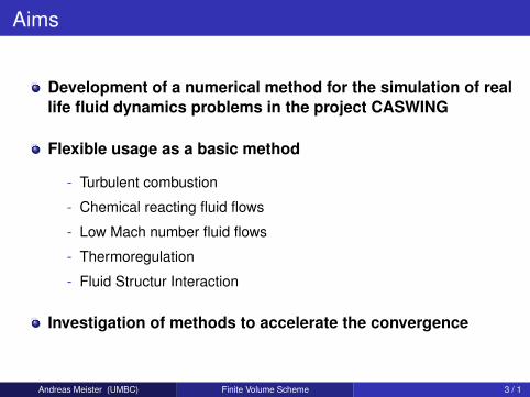
Aims
Development of a numerical method for the simulation of reallife fluid dynamics problems in the project CASWING
Flexible usage as a basic method
- Turbulent combustion
- Chemical reacting fluid flows
- Low Mach number fluid flows
- Thermoregulation
- Fluid Structur Interaction
Investigation of methods to accelerate the convergence
Andreas Meister (UMBC) Finite Volume Scheme 3 / 1
Aims
Requirements
- Flow dependent discretization of arbitrary complex geometries
- Taking account of moving boundaries
- Consideration of turbulence effects
- Minimization of computing time? Implicit scheme
? Preconditioned Krylov subspace methods
Andreas Meister (UMBC) Finite Volume Scheme 4 / 1
Balance laws
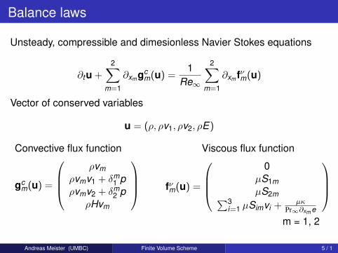
Unsteady, compressible and dimesionless Navier Stokes equations
∂tu +2∑
m=1
∂xmgcm(u) =
1Re∞
2∑m=1
∂xm fνm(u)
Vector of conserved variables
u = (ρ, ρv1, ρv2, ρE)
Convective flux function
gcm(u) =
ρvm
ρvmv1 + δm1 p
ρvmv2 + δm2 p
ρHvm
Viscous flux function
fνm(u) =
0
µS1mµS2m∑3
i=1 µSimvi + µκPr∞∂xm e
m = 1, 2
Andreas Meister (UMBC) Finite Volume Scheme 5 / 1

Finite Volume Method∫σ(t)
∂tu dx +2∑
m=1
∫σ(t)
∂xmgcm(u) dx =
1Re∞
2∑m=1
∫σ(t)
∂xm fνm(u) dx
Cell averages on a dual mesh
ui =1|σi |
∫σi
u dx
Gauß Integral Theorem and Reynolds Transport Theorem(Evolution equation for cell averages)
ddt
ui =1|σi(t)|
1Re∞
∫∂σi (t)
2∑m=1
fνm(u)nm ds −∫
∂σi (t)
2∑m=1
fcm(u)nm ds
fcm(u) = gc
m(u)− νnetz,mu
Andreas Meister (UMBC) Finite Volume Scheme 6 / 1
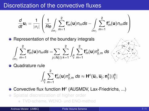
Discretization of the convective fluxes
ddt
ui =1|σi |
1Re
∫∂σi
2∑m=1
fνm(u)nmds −∫∂σi
2∑m=1
fcm(u)nmds
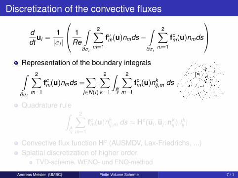
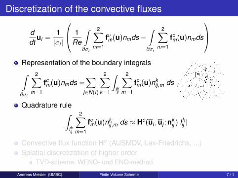
Representation of the boundary integrals∫∂σi
2∑m=1
fcm(u)nmds =
∑j∈N(i)
2∑k=1
∫lkij
2∑m=1
fcm(u)nk
ij,m ds
Quadrature rule∫lkij
2∑m=1
fcm(u)nk
ij,m ds ≈ Hc(ui ,uj ; nkij )|lkij |
Convective flux function Hc (AUSMDV, Lax-Friedrichs, ...)Spiatial discretization of higher order
TVD-scheme, WENO- und ENO-method
Andreas Meister (UMBC) Finite Volume Scheme 7 / 1
Discretization of the convective fluxes
ddt
ui =1|σi |
1Re
∫∂σi
2∑m=1
fνm(u)nmds −∫∂σi
2∑m=1
fcm(u)nmds
Representation of the boundary integrals∫∂σi
2∑m=1
fcm(u)nmds =
∑j∈N(i)
2∑k=1
∫lkij
2∑m=1
fcm(u)nk
ij,m ds
Quadrature rule∫lkij
2∑m=1
fcm(u)nk
ij,m ds ≈ Hc(ui ,uj ; nkij )|lkij |
Convective flux function Hc (AUSMDV, Lax-Friedrichs, ...)Spiatial discretization of higher order
TVD-scheme, WENO- und ENO-method
Andreas Meister (UMBC) Finite Volume Scheme 7 / 1
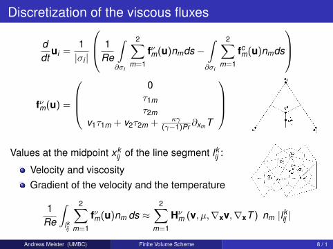
Discretization of the viscous fluxes
ddt
ui =1|σi |
1Re
∫∂σi
2∑m=1
fνm(u)nmds −∫∂σi
2∑m=1
fcm(u)nmds
fνm(u) =
0τ1mτ2m
v1τ1m + v2τ2m + κγ(γ−1)Pr ∂xmT
Values at the midpoint xk
ij of the line segment lkij :
Velocity and viscosityGradient of the velocity and the temperature
1Re
∫lkij
2∑m=1
fνm(u)nm ds ≈2∑
m=1
Hνm (v, µ,∇xv,∇xT ) nm |lkij |
Andreas Meister (UMBC) Finite Volume Scheme 8 / 1
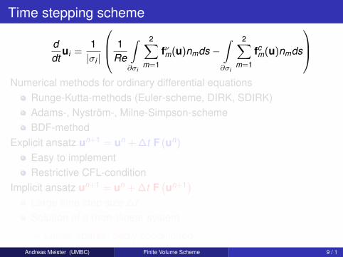
Time stepping scheme
ddt
ui =1|σi |
1Re
∫∂σi
2∑m=1
fνm(u)nmds −∫∂σi
2∑m=1
fcm(u)nmds
Numerical methods for ordinary differential equations
Runge-Kutta-methods (Euler-scheme, DIRK, SDIRK)Adams-, Nyström-, Milne-Simpson-schemeBDF-method
Explicit ansatz un+1 = un + ∆t F (un)
Easy to implementRestrictive CFL-condition
Implicit ansatz un+1 = un + ∆t F(un+1)
Large time step size ∆tSolution of a (non-)linear system
→ Large, sparse, badly conditionedAndreas Meister (UMBC) Finite Volume Scheme 9 / 1
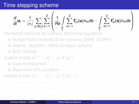
Time stepping scheme
ddt
ui =1|σi |
∑j∈N(i)
2∑k=1
1Re
∫lkij
2∑m=1
fνm(u)nmds −∫lkij
2∑m=1
fcm(u)nmds
Numerical methods for ordinary differential equations
Runge-Kutta-methods (Euler-scheme, DIRK, SDIRK)Adams-, Nyström-, Milne-Simpson-schemeBDF-method
Explicit ansatz un+1 = un + ∆t F (un)
Easy to implementRestrictive CFL-condition
Implicit ansatz un+1 = un + ∆t F(un+1)
Large time step size ∆tSolution of a (non-)linear system
→ Large, sparse, badly conditionedAndreas Meister (UMBC) Finite Volume Scheme 9 / 1
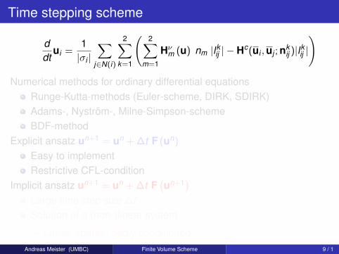
Time stepping scheme
ddt
ui =1|σi |
∑j∈N(i)
2∑k=1
2∑m=1
Hνm (u) nm |lkij | −
∫lkij
2∑m=1
fcm(u)nmds
Numerical methods for ordinary differential equations
Runge-Kutta-methods (Euler-scheme, DIRK, SDIRK)Adams-, Nyström-, Milne-Simpson-schemeBDF-method
Explicit ansatz un+1 = un + ∆t F (un)
Easy to implementRestrictive CFL-condition
Implicit ansatz un+1 = un + ∆t F(un+1)
Large time step size ∆tSolution of a (non-)linear system
→ Large, sparse, badly conditionedAndreas Meister (UMBC) Finite Volume Scheme 9 / 1
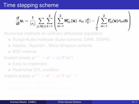
Time stepping scheme
ddt
ui =1|σi |
∑j∈N(i)
2∑k=1
(2∑
m=1
Hνm (u) nm |lkij | − Hc(ui ,uj ; nk
ij )|lkij |
)
Numerical methods for ordinary differential equationsRunge-Kutta-methods (Euler-scheme, DIRK, SDIRK)Adams-, Nyström-, Milne-Simpson-schemeBDF-method
Explicit ansatz un+1 = un + ∆t F (un)
Easy to implementRestrictive CFL-condition
Implicit ansatz un+1 = un + ∆t F(un+1)
Large time step size ∆tSolution of a (non-)linear system
→ Large, sparse, badly conditionedAndreas Meister (UMBC) Finite Volume Scheme 9 / 1
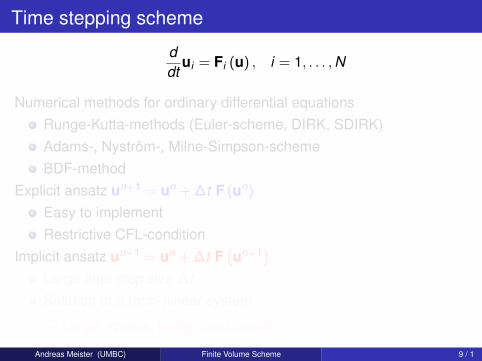
Time stepping scheme
ddt
ui = Fi (u) , i = 1, . . . ,N
Numerical methods for ordinary differential equationsRunge-Kutta-methods (Euler-scheme, DIRK, SDIRK)Adams-, Nyström-, Milne-Simpson-schemeBDF-method
Explicit ansatz un+1 = un + ∆t F (un)
Easy to implementRestrictive CFL-condition
Implicit ansatz un+1 = un + ∆t F(un+1)
Large time step size ∆tSolution of a (non-)linear system
→ Large, sparse, badly conditioned
Andreas Meister (UMBC) Finite Volume Scheme 9 / 1
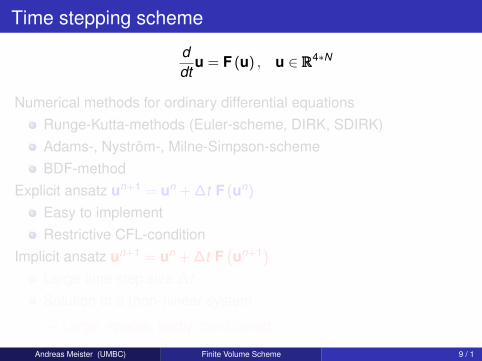
Time stepping scheme
ddt
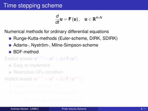
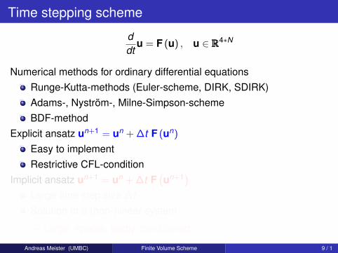
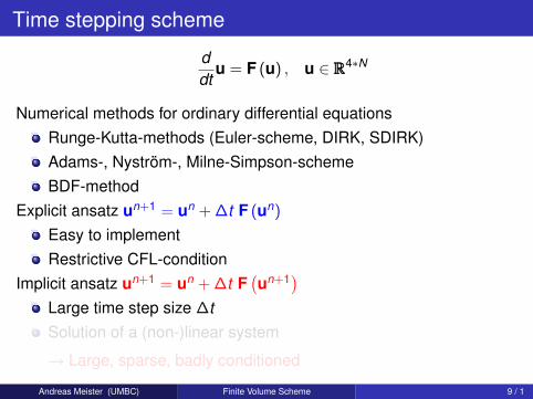
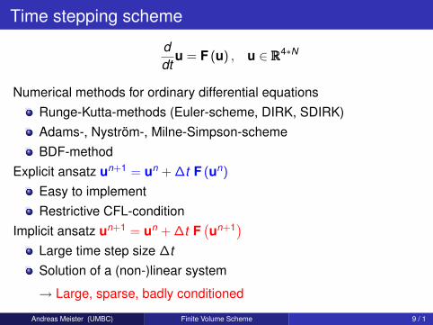
u = F (u) , u ∈ RRR4∗N
Numerical methods for ordinary differential equationsRunge-Kutta-methods (Euler-scheme, DIRK, SDIRK)Adams-, Nyström-, Milne-Simpson-schemeBDF-method
Explicit ansatz un+1 = un + ∆t F (un)
Easy to implementRestrictive CFL-condition
Implicit ansatz un+1 = un + ∆t F(un+1)
Large time step size ∆tSolution of a (non-)linear system
→ Large, sparse, badly conditioned
Andreas Meister (UMBC) Finite Volume Scheme 9 / 1
Time stepping scheme
ddt
u = F (u) , u ∈ RRR4∗N
Numerical methods for ordinary differential equationsRunge-Kutta-methods (Euler-scheme, DIRK, SDIRK)Adams-, Nyström-, Milne-Simpson-schemeBDF-method
Explicit ansatz un+1 = un + ∆t F (un)
Easy to implementRestrictive CFL-condition
Implicit ansatz un+1 = un + ∆t F(un+1)
Large time step size ∆tSolution of a (non-)linear system
→ Large, sparse, badly conditioned
Andreas Meister (UMBC) Finite Volume Scheme 9 / 1
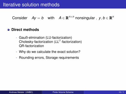
Iterative solution methods
Consider Ay = b with A ∈ RRRn×n nonsingular , y ,b ∈ RRRn
Direct methods
- Gauß-elmination (LU-factorization)Cholesky-factorization (LLT -factorization)QR-factorization
- Why do we calculate the exact solution?
- Rounding errors, Storage requirements
Andreas Meister (UMBC) Finite Volume Scheme 10 / 1
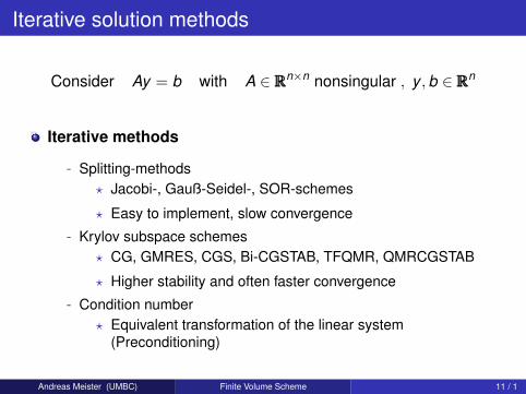
Iterative solution methods
Consider Ay = b with A ∈ RRRn×n nonsingular , y ,b ∈ RRRn
Iterative methods
- Splitting-methods? Jacobi-, Gauß-Seidel-, SOR-schemes
? Easy to implement, slow convergence
- Krylov subspace schemes? CG, GMRES, CGS, Bi-CGSTAB, TFQMR, QMRCGSTAB
? Higher stability and often faster convergence
- Condition number? Equivalent transformation of the linear system
(Preconditioning)
Andreas Meister (UMBC) Finite Volume Scheme 11 / 1
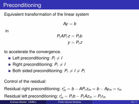
Preconditioning
Equivalent transformation of the linear system
Ay = b
inPlAPr z = Plb
y = Pr z
to accelerate the convergence.Left preconditioning: Pl 6= IRight preconditioning: Pr 6= IBoth sided preconditioning: Pr 6= I 6= Pl
Control of the residual:
Residual right preconditioning: r rm = b − APr zm = b − Aym = rm
Residual left preconditioning: r lm = Plb − PlAzm = Pl rm
Andreas Meister (UMBC) Finite Volume Scheme 12 / 1

Preconditioning
Incomplete LU-factorizationAdditional storage, time consuming calculationFrozen formulation, here ILU(p)
Splitting schemes (GS, SGS)No additional storageNo calculation
Scaling (Jacobi et. al.)Low additional storage, weak acceleration
Characteristic approachEigenvalues λ1/2 = v · n, λ3/4 = v · n + cRenumberingApplication of a splitting-based preconditionerCHASGS and CHAGS
Andreas Meister (UMBC) Finite Volume Scheme 13 / 1

Bi-NACA0012 Airfoil
Ma = 0.55, Angle of attack 6, inviscidTriangulation: 26632 triangles, 13577 points
Abbildung: Partial view of the triangulation w.r.t. the Bi-NACA0012 Airfoil anddensity distribution
Andreas Meister (UMBC) Finite Volume Scheme 14 / 1
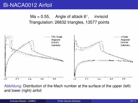
Bi-NACA0012 Airfoil
Ma = 0.55, Angle of attack 6, inviscidTriangulation: 26632 triangles, 13577 points
Abbildung: Distribution of the Mach number at the surface of the upper (left)and lower (right) airfoil
Andreas Meister (UMBC) Finite Volume Scheme 15 / 1
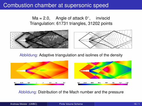
Combustion chamber at supersonic speed
Ma = 2.0, Angle of attack 0, inviscidTriangulation: 61731 triangles, 31202 points
Abbildung: Adaptive triangulation and isolines of the density
Abbildung: Distribution of the Mach number and the pressure
Andreas Meister (UMBC) Finite Volume Scheme 16 / 1

NACA0012-Airfoil
Ma = 0.85, α = 0, viscousRe = 500, T∞ = 273K , adiabatic
Abbildung: Partial view of the triangulation w.r.t. the NACA0012 Airfoil andisolines of the Mach number
Andreas Meister (UMBC) Finite Volume Scheme 17 / 1
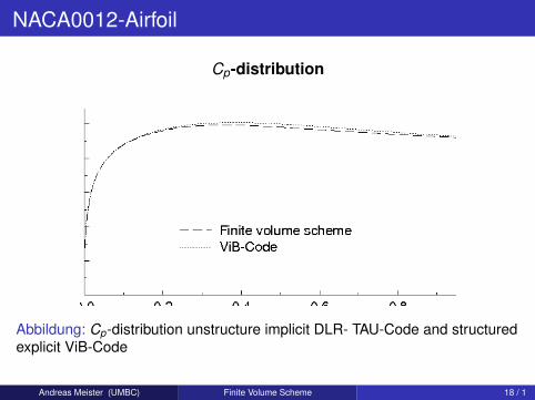
NACA0012-Airfoil
Cp-distribution
Abbildung: Cp-distribution unstructure implicit DLR- TAU-Code and structuredexplicit ViB-Code
Andreas Meister (UMBC) Finite Volume Scheme 18 / 1
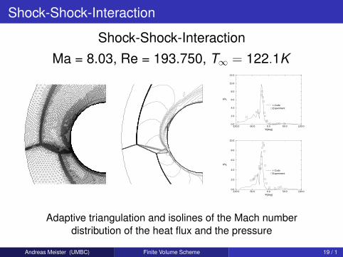
Shock-Shock-Interaction
Shock-Shock-InteractionMa = 8.03, Re = 193.750, T∞ = 122.1K
-100.0 -50.0 0.0 50.0 100.0Ψ[deg]
0.0
2.0
4.0
6.0
8.0
10.0
12.0
p/p0
τ-Code Experiment
-100.0 -50.0 0.0 50.0 100.0Ψ[deg]
0.0
2.0
4.0
6.0
8.0
10.0
q/q0
τ-CodeExperiment
Adaptive triangulation and isolines of the Mach numberdistribution of the heat flux and the pressure
Andreas Meister (UMBC) Finite Volume Scheme 19 / 1
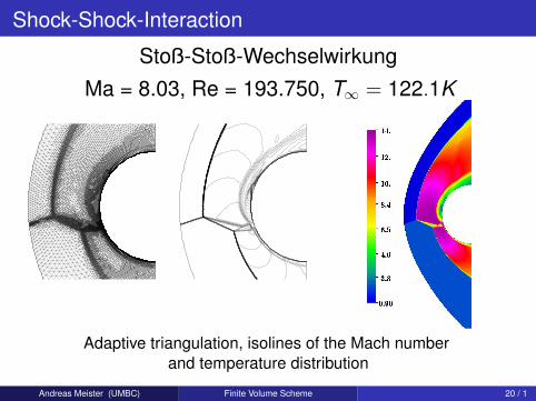
Shock-Shock-Interaction
Stoß-Stoß-WechselwirkungMa = 8.03, Re = 193.750, T∞ = 122.1K
Adaptive triangulation, isolines of the Mach numberand temperature distribution
Andreas Meister (UMBC) Finite Volume Scheme 20 / 1
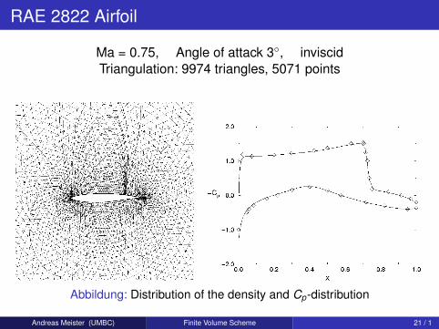
RAE 2822 Airfoil
Ma = 0.75, Angle of attack 3, inviscidTriangulation: 9974 triangles, 5071 points
Abbildung: Distribution of the density and Cp-distribution
Andreas Meister (UMBC) Finite Volume Scheme 21 / 1

RAE 2822 Airfoil
Ma = 0.75, Angle of attack 3, inviscidTriangulation: 9974 triangles, 5071 points
Explicit scheme Implicit scheme
Scaling Incomplete LU(5)
100 % 24,36 % 2,86 %
Tabelle: Percentage comparison of the computing time
Andreas Meister (UMBC) Finite Volume Scheme 22 / 1
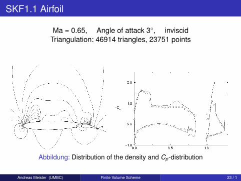
SKF1.1 Airfoil
Ma = 0.65, Angle of attack 3, inviscidTriangulation: 46914 triangles, 23751 points
Abbildung: Distribution of the density and Cp-distribution
Andreas Meister (UMBC) Finite Volume Scheme 23 / 1
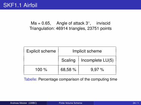
SKF1.1 Airfoil
Ma = 0.65, Angle of attack 3, inviscidTriangulation: 46914 triangles, 23751 points
Explicit scheme Implicit scheme
Scaling Incomplete LU(5)
100 % 68,58 % 9,97 %
Tabelle: Percentage comparison of the computing time
Andreas Meister (UMBC) Finite Volume Scheme 24 / 1
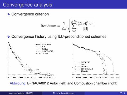
Convergence analysis
Convergence criterion
Residuum =14t
√√√√#Nh∑i=1
(4ρ)2i |σi ||Ω|
Convergence history using ILU-preconditioned schemes
Abbildung: Bi-NACA0012 Airfoil (left) and Combustion chamber (right)
Andreas Meister (UMBC) Finite Volume Scheme 25 / 1
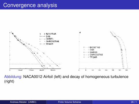
Convergence analysis
Abbildung: NACA0012 Airfoil (left) and decay of homogeneous turbulence(right)
Andreas Meister (UMBC) Finite Volume Scheme 26 / 1
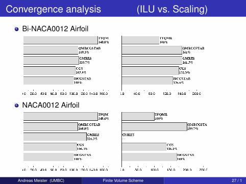
Convergence analysis (ILU vs. Scaling)
Bi-NACA0012 Airfoil
NACA0012 Airfoil
Andreas Meister (UMBC) Finite Volume Scheme 27 / 1
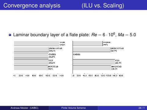
Convergence analysis (ILU vs. Scaling)
Laminar boundary layer of a flate plate: Re = 6 · 106, Ma = 5.0
Andreas Meister (UMBC) Finite Volume Scheme 28 / 1
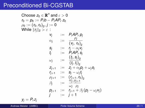
Preconditioned Bi-CGSTAB
Choose z0 ∈ RRRn and ε > 0r0 = p0 := Plb − PlAPr z0ρ0 := (r0, r0)2, j := 0While ‖rj‖2 > ε :
vj := PlAPr pj
αj :=ρj
(vj , r0)2sj := rj − αjvjtj := PlAPr sj
ωj :=(tj , sj )2(tj , tj )2
zj+1 := zj + αjpj + ωjsjrj+1 := sj − ωj tjρj+1 := (rj+1, r0)2
βj :=αj
ωj
ρj+1
ρjpj+1 := rj+1 + βj (pj − ωjvj )j := j + 1
yj = Pr zj
Andreas Meister (UMBC) Finite Volume Scheme 29 / 1
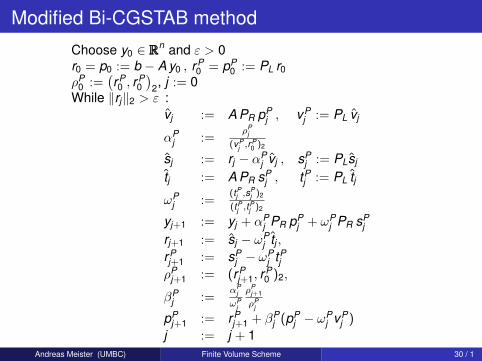
Modified Bi-CGSTAB method
Choose y0 ∈ RRRn and ε > 0r0 = p0 := b − A y0 , rP
0 = pP0 := PL r0
ρP0 :=
(rP0 , r
P0
)2, j := 0
While ‖rj‖2 > ε :vj := A PR pP
j , vPj := PL vj
αPj :=
ρPj
(vPj ,r
P0 )2
sj := rj − αPj vj , sP
j := PLsj
tj := A PR sPj , tP
j := PL tj
ωPj :=
(tPj ,s
Pj )2
(tPj ,t
Pj )2
yj+1 := yj + αPj PR pP
j + ωPj PR sP
jrj+1 := sj − ωP
j tj ,rPj+1 := sP
j − ωPj tP
jρP
j+1 := (rPj+1, r
P0 )2,
βPj :=
αPj
ωPj
ρPj+1
ρPj
pPj+1 := rP
j+1 + βPj (pP
j − ωPj vP
j )
j := j + 1Andreas Meister (UMBC) Finite Volume Scheme 30 / 1
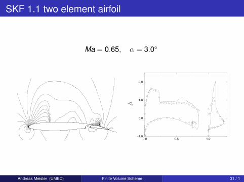
SKF 1.1 two element airfoil
Ma = 0.65, α = 3.0
0.0 0.5 1.0−1.0
0.0
1.0
2.0
−Cp
Andreas Meister (UMBC) Finite Volume Scheme 31 / 1
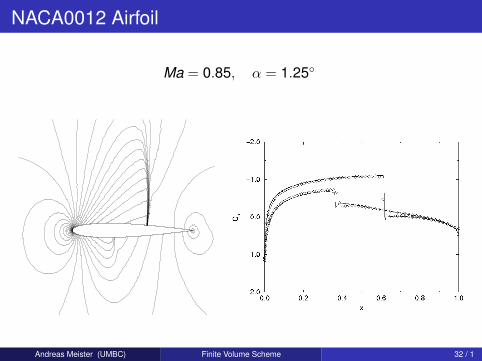
NACA0012 Airfoil
Ma = 0.85, α = 1.25
Andreas Meister (UMBC) Finite Volume Scheme 32 / 1

Comparison of Preconditioners
SKF 1.1 two element airfoil; Ma = 0.65, α = 3.0
D1(r) D2(r) D∞(r) DJac(r) DJac(l)1038% 953% 992% 438% 514%
NACA0012 Airfoil Ma = 0.85, α = 1.25
Andreas Meister (UMBC) Finite Volume Scheme 33 / 1
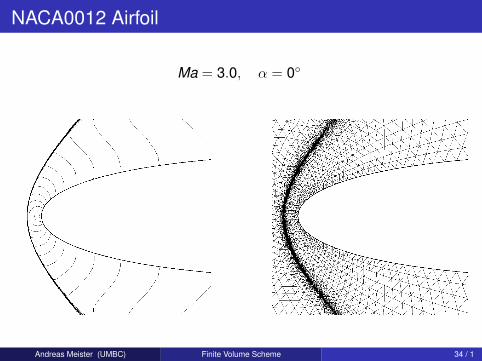
NACA0012 Airfoil
Ma = 3.0, α = 0
Andreas Meister (UMBC) Finite Volume Scheme 34 / 1
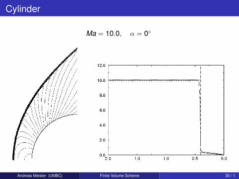
Cylinder
Ma = 10.0, α = 0
Andreas Meister (UMBC) Finite Volume Scheme 35 / 1

Comparison of Preconditioners
NACA0012 Airfoil Ma = 3.0, α = 0
Cylinder Ma = 10.0, α = 0
Andreas Meister (UMBC) Finite Volume Scheme 36 / 1
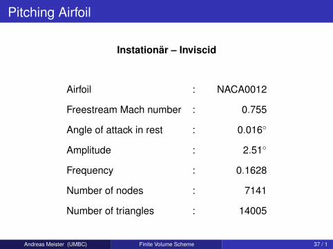
Pitching Airfoil
Instationär – Inviscid
Airfoil : NACA0012
Freestream Mach number : 0.755
Angle of attack in rest : 0.016
Amplitude : 2.51
Frequency : 0.1628
Number of nodes : 7141
Number of triangles : 14005
Andreas Meister (UMBC) Finite Volume Scheme 37 / 1
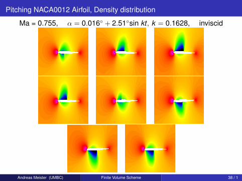
Pitching NACA0012 Airfoil, Density distribution
Ma = 0.755, α = 0.016 + 2.51sin kt , k = 0.1628, inviscid
Andreas Meister (UMBC) Finite Volume Scheme 38 / 1

Pitching NACA0012 - Airfoil, Cp-distribution
Ma = 0.755, α = 0.016 + 2.51sin kt , k = 0.1628, inviscid
Andreas Meister (UMBC) Finite Volume Scheme 39 / 1
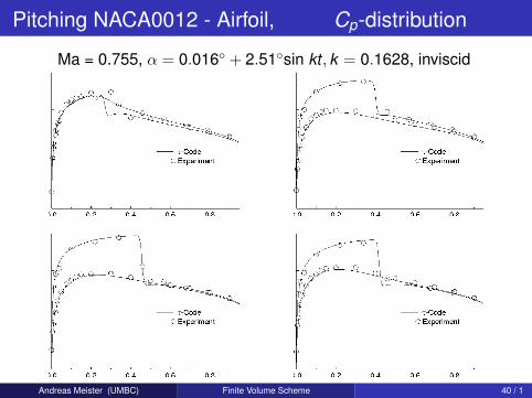
Pitching NACA0012 - Airfoil, Cp-distribution
Ma = 0.755, α = 0.016 + 2.51sin kt , k = 0.1628, inviscid
Andreas Meister (UMBC) Finite Volume Scheme 40 / 1

Pitching NACA0012 - Airfoil, Lift and Momentum
Lift coefficient Momentum coefficient
Andreas Meister (UMBC) Finite Volume Scheme 41 / 1
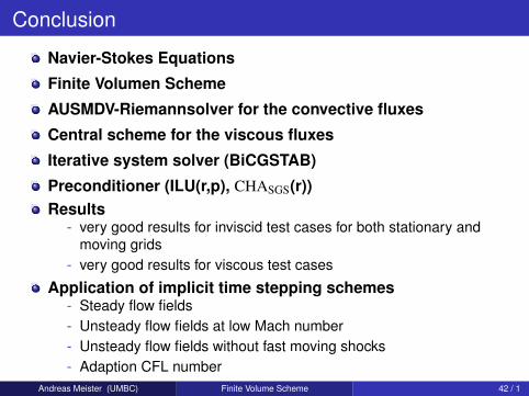
Conclusion
Navier-Stokes Equations
Finite Volumen Scheme
AUSMDV-Riemannsolver for the convective fluxes
Central scheme for the viscous fluxes
Iterative system solver (BiCGSTAB)
Preconditioner (ILU(r,p), CHASGS(r))Results
- very good results for inviscid test cases for both stationary andmoving grids
- very good results for viscous test cases
Application of implicit time stepping schemes- Steady flow fields- Unsteady flow fields at low Mach number- Unsteady flow fields without fast moving shocks- Adaption CFL number
Andreas Meister (UMBC) Finite Volume Scheme 42 / 1


![Implicit Finite Element Schemes for the Stationary Compressible … · Implicit Finite Element Schemes for the Stationary Compressible ... [32] overwrite the boundary integral by](https://img.dokumen.tips/doc/110x75/5b83ed847f8b9a315b8e3072/implicit-finite-element-schemes-for-the-stationary-compressible-implicit-finite.jpg)