Explicit-Implicit Schemes for the Numerical Solution of ... increased stability range for the implicit schemes are unfortunately offset by two important disadvantages. First, the implicit

MATHEMATICS OF COMPUTATION, VOLUME 29, NUMBER 130

APRIL 1975, PAGES 407-424

Explicit-Implicit Schemes for the Numerical Solution

of Nonlinear Hyperbolic Systems

By G. R. McGuire and J. Ii. Morris

Abstract. A class of methods, comprising combinations of explicit and implicit methods,

for solving systems of conservation laws in one space dimension is developed. The ex-

plicit methods of McGuire and Morris [S] are combined with the implicit methods of

McGuire and Morris [11] in a manner similar to that for creating Hopscotch methods

(Gourlay [13]). The stability properties of these explicit-implicit methods is investigat-

ed and the results of some numerical experiments are presented. Extensions of these

methods to systems of conservation laws in two space dimensions are also briefly dis-

cussed.

1. Introduction. We will consider finite-difference methods for solving systems of

conservation laws of the form

(1.1) bulbt + bf(u)lbx = 0

defined on the region G = {0 < x < X} x {t > 0} where u and / are «-vectors. Equa-

tion (1.1) is assumed to be hyperbolic in G, which means that the Jacobian A(u) =

bf(u)lbu has everywhere real eigenvalues and a complete set of linearly independent ei-

genvectors. The eigenvalues of A(u) are further assumed to be positive, so that system

(1.1) subject to initial conditions

0-2) W(*. fj) = /(x)and boundary conditions

(1.3) u(0,t) = g(t)

is well posed. A full account of the theoretical aspects of this problem may be found

in Jeffrey and Tanuiti [1] (see also Olelnik [2]).

In the usual manner, we assume a uniform discretization of G by a mesh parallel

to the coordinate axes with a mesh spacing h in the x coordinate and k in the time di-

rection. We denote by (ih, mk) the nodal points of the mesh where, without loss of

generality, we assume X = Nh so that / ranges over the integers 0, 1, 2, • • -, N and m

takes integer values 0, 1, 2, • • •.

We denote by um = u(ih, mk) the solution of (1.1) at (ih, mk) and by w™ =

w(ih, mk) an approximation to um. We assume the mesh ratio p (= klh) is constant.

There is, in existence, a large number of methods for solving system (1.1). Most

of the difference methods proposed to date have been second-order accurate explicit

methods (see Lax and Wendroff [6], Richtmyer [3], Gourlay and Morris [4], Burstein

Received November 19, 1973.

AMS(MOS)subject classifications (1970). Primary 65M05, 65M10.

Copyright © 1975, American Mathematical Society

407

License or copyright restrictions may apply to redistribution; see http://www.ams.org/journal-terms-of-use

408 G. R. MCGUIRE AND J. LI. MORRIS

and Rubin [24], McGuire and Morris [5]), although the lesser accurate methods of Lax

[7] and Hopscotch-Lax [17] are also of interest. A three-level difference scheme which

is particularly useful for solving systems of the form (1.1) over long time intervals is the

leap-frog method

(1.4) *7 + ï=™?~l-p[f?+i-f?-xl

A full discussion of many of these methods may be found in Richtmyer and Morton

[8]; see also the comprehensive bibliography contained in Roache [25].

An important feature of explicit difference methods for hyperbolic equations is

that they must satisfy the classical Courant-Friedrichs-Lewy (CFL) convergence condi-

tion (see [9]). This condition imposes a restriction on the mesh ratio p. Hence, for a

given h, the time step k is restricted in size. For nonlinear systems, in order to imple-

ment the CFL condition, it is necessary to consider the linearized versions,

(1.5) bu/bt + A bulbx = 0,

of (1.1) where A is a constant matrix. Since consistency is a prerequisite of the differ-

ence methods for the solution of (1.1), stability and convergence are equivalent for lin-

ear problems by virtue of Lax's equivalence theorem (see Richtmyer and Morton [8]).

This, of course, only applies to linear problems and, in any case, stability is not defined

in the nonlinear case. Stability is analysed for difference schemes applied to (1.5) using

the usual Fourier analysis (see [8]). This analysis requires an investigation of the ampli-

fication matrix of the difference approximation. The Von Neumann necessary condi-

tion requires that the eigenvalues of this matrix be bounded by one in modulus. All

the schemes considered have amplification matrices which are rational functions of A

and, hence, since (1.5) is assumed hyperbolic, these amplification matrices are uniform-

ly diagonalizable which means that the Von Neumann condition is sufficient as well as

necessary for stability (see [8]).

An additional important property required of difference methods for nonlinear

hyperbolic systems is that their linearized versions (the methods applied to (1.5)) be

dissipative in the sense of Kreiss; namely, dissipative of order 2r (r is a positive integer)

means that there exists a ô > 0 such that

(1.6) I/(b)K1 - old2' VIoKtt

where / is an eigenvalue of the amplification matrix and a is the Fourier variable.

In considering ways of alleviating stability restrictions associated with explicit

methods, we are naturally drawn to considering implicit methods and their (usually)

larger ranges of stability for the approximate solution of (1.1). Such implicit methods

have received less attention than explicit methods; see, however, Gary [10], Gourlay

and Morris [4], Abarbanel and Zwas [12], McGuire and Morris [11]. The advantages of

an increased stability range for the implicit schemes are unfortunately offset by two

important disadvantages. First, the implicit methods require either that a system of

nonlinear equations be solved or an iterative procedure be applied at each time step.

Second, with the exception of the method described in [11], the implicit methods are


NUMERICAL SOLUTION OF NONLINEAR HYPERBOLIC SYSTEMS 409

nondissipative and hence of dubious value for nonlinear hyperbolic systems in which

discontinuities can occur.

Our aim in this paper is to combine explicit and implicit methods in an endeavour

to produce schemes which possess properties approaching the best possible of the con-

stituent methods. Namely, the resulting scheme will preserve the dissipation and ease

of solution associated with the explicit methods whilst retaining an optimal stability by

virtue of the implicit methods.

Such an approach has already been successfully implemented for parabolic differ-

ential equations in a series of papers on the hopscotch methods; see Scala and Gordon

[16], Gourlay [13], Gourlay and McGuire [14]. In these papers, an explicit method and

its precise implicit version were combined so that the complete procedure could be lik-

ened to an ADI method. Hopscotch methods have also been derived for the system

(1.1) in Gourlay and Morris [17] and Gourlay, McGuire and Morris [18]. In the pres-

ent paper, however, we will adopt a slightly different approach in that classes of ex-

plicit and implicit second-order accurate methods are combined to give workable algo-

rithms satisfying our main requirements.

The method of combination and the resulting methods are described in the next

section. In Section 3, a stability analysis of the explicit-implicit methods is given. Sec-

tion 4 contains a description of numerical experiments carried out on the novel meth-

ods. In the final section, a brief account of extensions of the methods to two space

variables is given.

2. Second-Order Accurate Explicit-Implicit Schemes. In this section, we combine

two classes of second-order accurate explicit and implicit methods for solving system

(1.1) to give a class of explicit-implicit methods. We consider the class of explicit

schemes introduced in McGuire and Morris [5], namely

(2.1) wm+a = « * + <%)/2 - ap(/r+Vt -f™vJ,

(2-2) < + l= wm _| |£ _ JL) ifmj - fm¿ + !$■+. -/&■)],

where a =£ 0 and wm+a is a first-order approximation to um+a.

It was shown in [5] that the scheme (2.1), (2.2) is second-order accurate and sta-

ble in the linearized sense if

(2.3) pIXKl

where IXI is the maximum modulus eigenvalue of A. Further, it was shown that the

class of schemes was dissipative of order 4 in the linearized sense, provided

(2-4) 0<plXKl

for all eigenvalues X of A.

The class of implicit methods, which we shall consider, are the extensions of (2.1),

(2.2) given in McGuire and Morris [11]. Namely, (2.1) is taken with



(2.5)

wm+i =w™-f[(fc + d(a-!))(/£ ,-/£?!)

+ (% - «otfftî l-fT-tl) + ™U?Aa - /££•)]■

In [11], (2.1) and (2.5) are shown to be second-order accurate and stable provided

(2.6) ad>0 and plXI < l/\/2äd,

where IXI is the maximum modulus eigenvalue of A. The case ad = 0 gives the Crank -

Nicolson scheme and hence unconditional stability. The class of methods was also

shown to be dissipative of order 4, provided

(2.7) ad>0, 0<p\X\<l/y/2^d

for all eigenvalues X of A. ad = V¡ gives the class of explicit methods (2.1), (2.2).

Consider the following combination of these two classes of method:

(2 g\ Use (2.1), (2.2) at grid points with m + i odd

and then use (2.1), (2.5) at the other grid points.

Method (2.8) is called the explicit-implicit class of methods or, simply, the expli-

cit-implicit method. It is easily seen that the method is computationally explicit; for

application of (2.1), (2.2) at odd points of time level m (grid points with m + i odd)

then makes the application of the implicit method (2.1), (2.5) at this time level an ex-

plicit process. Also, (2.8) is not a Hopscotch method since (2.1), (2.5) is not the im-

plicit version of (2.1), (2.2).

Diagramatically, the explicit method uses the points depicted thus

(/, m + 1)

(/ - 1, m) (i, m) (i + 1, m)

whereas the implicit method uses the following points

(i - 1, m + 1) (/', m + 1) (/ + 1, m + 1)

(/*- l, m) (i, m) (i + l, m)

The combined method uses the points in the following way



where X denotes the use of the explicit method, and D denotes the use of the implicit

method.

Finally, it is obvious that the explicit-implicit scheme (2.8) is second-order accu-

rate. For, both the explicit and implicit schemes have local truncation errors 0(k3)

and, hence, so does the combination (2.8).

3. Stability Analysis of the Explicit-Implicit Schemes. In this section, we consider

the linearized version of (2.8) and analyse the stability properties of the method. Lin-

earizing Eqs. (2.1), (2.2) and eliminating the intermediate values, we obtain

(3-D w m + l _ wm pAf2A2

P*A« , - <?,) + ̂ f- (w£, - 2< + <!,).

Similarly, linearizing (2.1), (2.5) and eliminating starred values gives

„« +1 = wm _ e4(v4 _ ad)(w™ + » - w« + ») - Báty + ad)(w™ x - wmi}wi

(3.2)+ adp2A2(wm_ï - 2wf + w£,).

Now consider the application of method (2.8) at a point with m + i odd. Then

the points (/ 4- 1, m) and (i - 1, m) are even points and it is easily shown, by applying

(3.1) with m = m - 1, i = / + 1 and i = i - \, that

Mí#, -<-x = [/-p^kwîïï1 -wjür1)-^'«1 -2wr! +»íV)

(3.3)

and

(3.4)

+ ey-2«+21-<2"1)

vví+i + <i = [/-^2i(wr+v +vv,íür1)

+ e^-2(w-21 +2VV--1 +W-21)

-—(vi;m_1 - wm_1^

2 ^Wi+2 Wi-2 ¡

Now (i, m) is an odd point and so (3.2) gives w¡" there with m = m - \. Multiplying

this equation by [/ - p2A2], we then obtain



[I-p2A2]w¡" = [I-p2A2]w™-1 -p^[I-p2A2](^+ad)(w^+ll -w™"1)

(3-5) + adp2A2[I - p2A2](w¡"+-1 +w^~1)

-2adp2A2[I-p2A2]w?7-1.

Now, Eqs. (3.3) and (3.4) can be used to eliminate w™^1, w™^1 from (3.5). The re-

sulting expression then gives [I-p2A2]w™ as a function of only w™-1, wmx, w["2 l.

Finally, (m + 1, /') is an even point whose values are given by (3.1). Thus

(3.6) w? + l = [I-p2A2]w™ -P~(w^x -w^)+^(Wp+1 +W&).

Eliminating [/ - p2A2]w™, using (3.5) with w™^1 eliminated, gives

< +' = [' - \p2A2 - \adp2A2 + adp4A*\ w,™"1

~[pA-P-f(\-a^)]«+i-<-i)

+ P2A2{\ + ad) (**, + w^)+p3A3 (| + \ad) {wftf - wfr)(3.7)

,p2A2 Q + ad)I + 2adp2A2J (w™~21 + w£~l).4

The scheme (3.7) uses only values at the even points

w? + 1, wg,, wf*-\ WS,1.

Hence, the original explicit-implicit scheme, when linearized, is equivalent to an applica-

tion of (3.7) at points with (m + i) odd, with the values for (m + i) even filled in us-

ing the implicit scheme (3.2). Hence, basically the stability of (3.8) is determined by

the stability of Eq. (3.7). The advantage of the explicit-implicit scheme in the form

(3.8) is that the procedure is self-starting after print-outs whereas Eq. (3.7) used on

its own (only for linear equations), being a three-level scheme, requires a special start-

ing procedure.

The usual Fourier analysis applied to (3.7) gives an amplification matrix all of

whose eigenvalues must be less than unity in modulus before (3.7) can be stable. The

amplification matrix of (3.7) is a matrix whose terms are polynomials in A. This means

that, since A has linearly independent eigenvectors, the amplification matrix is uniform-

ly diagonalizable and so Von Neumann's condition is sufficient as well as necessary for

stability.

The eigenvalues p of the amplification matrix are given by replacing A in Eq.

(3.7) by one of its eigenvalues X (say), w¡¡" + 1 by p2, vvj"-1 by 1, w™ j - w™l by

2v/rïp sin a, w™ , + wjü, by 2p cos a, w™~21 - w™'1 by 2y^lsin 2a, and w™'1 +



w™2 ' by 2 cos 2a. This then gives

p2 + ( pX -P-2—\2 ~ adj) 2v^ P sin a - p2X2 (- + ad) 2p cos a

(3.8) - (l - |p2X2 - \adp2X2 + adp4X4) -p3X3( | + |a/) 2^1 sin 2a

+ ~- (( | + adj + 2adp2X2) 2 cos 2a = 0,

where a is the variable in the Fourier space corresponding to ih. Defining

^(pX, a) = -2p2X2(- + ad) cosa,

B(pX, a) = (pX - P-J-\\- adj) 2 sin a,

(3-9) cXpX, a) = - (l - |p2X2 - \adp2X2 + adp^X*)

+ P-^- ((^ + adj + 2adp2X2) 2 cos 2a,

D(pX, a) = -2p3X3 Q + |at?j sin 2a,

we find that Eq. (3.8) becomes

(3.10) p2 +(A +\f:lB)p+(C + yflD) = 0.

To prove that the explicit-implicit scheme is stable, we require to show that the

roots of (3.10) lie inside or on the unit circle. It is no easy problem to find conditions

on pX such that this is true. The first observation is that the scheme (3.7) is an explic-

it three-level scheme and, as such, is subject to the CFL condition for convergence. It

is easy to see that the condition, in this case, requires

(3.11) plXKl.

Further, since the scheme is consistent and the linearized system of differential equa-

tions (1.1) is well posed, the Lax-Richtmyer equivalence theorem gives (3.11) as a nec-

essary condition for stability of (3.7). Hence, by the equivalence of stability and the

Von Neumann condition for this scheme, the roots of (3.10) will have modulus greater

than one for some a when plXl is taken greater than one. Thus, we need only consider

values of pX in [-1, 1].

Replacing pX by -pX in (3.10) gives

(3.12) p2 +(A-^lB)p+(C-yfrlD) = 0.

If p is a root of (3.10), then p is a root of (3.12) and, since Ipl = Ipl, we need only

consider the moduli of the roots of Eq. (3.10) for pX in the interval [0, 1].

In a similar way, we can show that p(-a) satisfies (3.12). Hence

(3.13) p(a) = p(-a) for any a.



Also, since

.4(pX, 7T - a) = -A(pX, a), B(pX, n - a) = B(pX, a),

(3.14)C(pX, 7T - a) = C(pX, a), D(pX, tt - a) = ~D(pX, a),

we have that, if p(a) satisfies (3.10), then

P2(tt - a) + (-A + y/z~\B)p(n - a) + C - sflD = 0and so

(-p(7r - a))2 + (A + yfr\B)(-p(n - a)) + C + yf^D = 0.

Hence, p(a) and -p(7r - a) are the roots of (3.10). Thus, since these roots have the

same modulus, it is only necessary for us to consider the roots for a G [—tt/2, tt/2], and,

by (3.13), it is enough to consider both roots for a S [0, 7r/2] in order to determine the

maximum modulus for the roots of (3.10).

A full investigation as to which conditions on pX and ad give stability, is extreme-

ly complicated. However, a partial analysis can be carried out in the following manner.

By putting pX = 1 in (3.10), an investigation as to which values of ad give an optimal-

ly stable method can be performed.

In this case,

A(pX, a) = ,4(l,a)=M(a) = -(l +2ac?)cosa,

5(a) = (3/2 + a<i)sin a,

(3.16)C(a) = -04 - ad/2) + fcfli + 3ad)cos 2a,

D(a) = - 04 + 3ad/2)sin 2a.

The following theorem due to Miller [19] will be used.

Theorem 3.1. Let f be a polynomial of degree n and f its derivative with re-

spect to p, the dependent variable. Also, let

(3.17) /, (%) = (/*(0)/(?) - f(Q)f\mbe the reduced polynomial where

(3.18) /*(£) =- £27(l/ö-

Then fis a Von Neumann polynomial (all its roots lie on, or inside, the unit circle) iff

either

l/*(0)l> 1/(0)1

and /j is a Von Neumann polynomial

or

/j = 0 and f is a Von Neumann polynomial.

When

f(p) = p2 + (A + y/=lB)p +(C + y/^W),it is easily shown that

/*(p) = (C - \T~W)p2 +(A- \^l£)p + 1,

(3.19) /*(0) =1, f(0)=C + ^FlD,

fi(p)=(l -C2 -D2)p +(A - AC - BD) + sF~\(B - AD + BQ.



Lemma 3.2. With A, B, C, D given by (3.16),

A - AC - BD = -c cos ag(c, a),

(3.20) B - AD + BC = c sin CLg(c, a),

l-C2 -D2 = cg(c, a),

where g(c, a) = (2 - c) + (2 - 3c) cos2a and c = $4 - ad.

Proof. With c = $4 - ad, Eq. (3.16) becomes

A(a) = 2(c - 1) cos a, 5(a) = (2 - c) sin a,

C(a) = -c/2 + $4(2 - 3c) cos 2a, Z)(a) = - $4(2 - 3c) sin 2a.Thus

1 - C2 - D2 = (c/2)(6 - 5c 4- (2 - 3c) cos 2a) = c((2 - c) + (2 - 3c) cos2a),

A - AC - BD = 2(c - 1) cos a + c(c - 1) cos a - (2 - 3c)(c - 1) cos a cos 2a

+ $4(2 - c)(2 - 3c) sin a sin 2a = —c cos a{(2 - c) + (2 - 3c) cos2a}

and

B - AD + BC = (2 - c) sin a + (c - 1)(2 - 3c) cos a sin 2a

+ (-(c/2)(2 - c) sin a + $4(2 - c)(2 - 3c)sin a cos 2a)

= c sin a{(2 - c) + (2 - 3c) cos2a},

which proves the lemma.


/, = 0 Va iff c = 0.Proof.

fx = 0 Va iff 1 - C2 - D2 = 0,

/I -AC-BD =0,

5 - AD + BC = 0, Va iff c = 0,by Lemma 3.2.


l/*(0)l> 1/(0)1 Va iff 0<c<l.

Proof.

l/*(0)l> 1/(0)1 Va,

iff 1 -C2 -Z)2 >0 Va by (3.19),

iff cg(c, a) > 0 Va by Lemma 3.2.

Now when c < 0, g(c, a) > 0 Va and so cg(c, a) < 0 Va. Hence, cg(c, a) > 0 Va iff

c > 0 and g(c, a) > 0 Va. Now,



g(c, a) - 2(1 + cos2a) - c(l +3 cos2a) > 0 Va

2(1 + cos2 a) wiff c < —*-*- Va,

1+3 cos2a

•ff ^ • 2(1 + x)uf c < min , i o = 1 •

xe|o,i] ! + •>•*

Hence the lemma is proved.

The following remarks are useful.

Remark 1. l/*(0)l > 1/(0)1 Va ¥= 0 iff 0 < c < 1.

The proof is almost that of the lemma except that Va is replaced by Va =£ 0

and we have

g(c, a) > 0 Va # 0,

... . 2(1 + cos2a) u ,iff c < -^-— Va + 0,

1 + 3 cos2a

iff c < 1, on taking limits as a —► 0.

Remark 2. When a = 0, f(p) has roots 1, 1 - 2c and so f(p), with a = 0, is a

Von Neumann polynomial iff 0 < c < 1.

The following theorem can now be proved.

Theorem 3.5. The explicit-implicit scheme is stable in the linearized sense for

p\X\= 1 iff-1/i<ad<lA.

Proof.

f(p) is a Von Neumann polynomial Va,

iff /(p), for a G ]0,7r/2], is Von Neumann and /(p) for a = 0 is

Von Neumann,

iff either l/*(0)l > 1/(0)1 and fx is Von Neumann,

or /j =0 and /' is Von Neumann for all a G ]0,7r/2] and /(p)

for a = 0 is Von Neumann,

.ffn, ., , (A-AC-BD)2 +(B-AD+BQ2 , . w , .iff 0 < c < 1 and ^-L-l— < 1 Va ^ 0

(1 -C2 -D2)2

with c G ]0, 1], using Remark 1,

orc = 0 and (A2 + B2)/4 < 1 for a ¥= 0 with c = 0,

and 0 < c < 1 by Remark 2.

Now (A-AC- BD)2 +(B-AD+ BC)2 = c2g2(c, a) by Lemma 3.2 and (1 - C2 -

D2)2 = c2g2(c, a) > 0 for a ¥= 0 and c G ]0, 1 ]. Hence

(A-AC- BD)2 +(B-AD + BC)2 . , ,_ ... ..1-'--*-'— =1 for a ^ 0 and 0 < c < 1.

(l-C2-£>2)2Also

(A2 + B2)/4 = 1 when c = 0.

Hence, the theorem is proved.



If it can be assumed that if the scheme is stable for p IXI = 1 then it is stable for

all smaller time steps, namely p IXI < 1, then the nice result

'optimal stability is achieved iff -$4 < ad < $4',

can be obtained.

To derive this result analytically is extremely difficult. Thus, a computer search

was made on the roots of (3.10) for a in [0,7r/2] and pX in [0, 1] and for a range of

values of ad. The results are given in Table 3.1.

Table 3.1.

p\ = maximum value of pX in the range .1(.1)1.0, and for which the moduli of the

roots of Eq. (3.10) for all a in the range 0{nl\QQ)nl2, are < 1.

ad

P\

<-.52

<.l

-.5

to .5

1.0

.52

to .7

.9

.8, .9, 1.0 2.0

.6

3.0

.5

>4.0

<.5

From Table 3.1, optimal stability is only achieved (as given by Theorem 3.5) for

ad G [- $4, Ví]. The remarkable feature of these results is the fact that, just below

ad = - .5, the range of stability is drastically reduced, while, for values of ad above .5,

the range of stability falls off more slowly.

A corollary to Theorem 3.5 can be proved with the aid of another theorem due

to Miller [19], namely:

/is a Schur polynomial (all its roots lie inside the unit circle) iff l/*(0)l >

1/(0)1 and /j is a Schur polynomial.

Corollary 3.6. For the explicit scheme to be dissipative in the linearized sense,

it is required that p \X\< 1.

Proof. From the proof of Theorem 3.5, l/*(0)l is not greater than 1/(0)1 for c =

0, 1 when pX = 1. Also, for 0 < c < 1, fx is not a Schur polynomial when pX = 1.

Thus, since for a dissipative scheme / is required to be a Schur polynomial, the corol-

lary is proved.

4. Numerical Experiments in One Space Dimension. In this section, the results of

some numerical experiments carried out using the explicit-implicit scheme (3.8) are pre-

sented. In all the experiments, we used the scalar equation

(4.1) bulbt + (b/bx)(Yiu2) = 0

in the region {0 < x < 1} x {r > 0}. The experiments were of two kinds; the first set

consisted of problems with smooth solutions while the second set was on a problem

with a discontinuous solution. For the smooth problems, we used the following sets of

stability values and boundary conditions:

(4.1al) (a) u(x, 0)

(4.1aII)

x,

u(0, t) = 0,


418 G. R. MCGUIRE AND J. Ll. MORRIS

(4.1bl) (b) u(x,0) = x2

and boundary condition (4.1 ail),

(4.Ici) (c) u(x, 0) = \/x

and (4.1 ail).

These problems have the smooth solutions

(4.1aIII) (a) u(x, t) = x/(l + t),

i a iunn cw\ í a 1 + 2xr - VI + Axt(4.1bIII) (b) u(x, t) =-*-2r2

(4.1CIII) (c) M(M)=-Í+V/Í2

2

respectively. The results, using the Eqs. (a), (b) and (c), are given in Tables 4.1(a, b, c),

respectively. Backward difference versions of the explicit and implicit schemes were

used to give values at the grid points on the upper boundary x = 1 (see [5], [11]). Ten

grid points were used on [0, 1] so that h = 0.1. Errors at a central grid point, after

300 time steps, are given in the tables for a series of values of a and d and for a selec-

tion of values of p.

The maximum value of the solution in experiment (a) is 1, and this occurs at

t = 0 with the solution decreasing with increasing time. Thus, optimal stability occurs

for p = 1. From Theorem 3.5 and remarks following it, optimal stability should occur

only for - $4 < ad < $4. The results in Table 4.1(a(i)) indicate that the scheme is stable

over a larger range of positive ad. It is to be noted, however, that the solution does

decrease with increasing time and hence the local optimal stability condition is not p =

1 as time increases.

Similar remarks apply to Tables 4.1(b, c(i)). Also, from a comparison of Tables

4.1(i) and (ii) in all cases (a), (b) and (c), it is observed that instability occurs for a

larger range of ad when p = 1.0, than when p = 0.5 as would be expected from the re-

sults of the computer search. Notice also, in all cases (a), (b) and (c), the extremely

small truncation errors. A truncation error analysis would give best values of a and d

for minimizing truncation errors.

In the second set of numerical experiments, the discontinuous initial values

(1, 0<x<.l,(4-ldI) u(x, 0) = I

(o, x> A,and boundary condition

(4.1dH) «(0, r)=l (r > 0)

were used. In this case, (4.1) has the discontinuous solution in which the discontinuity

of (4.1dl) is propagated into the field of solution along the line x = 0.1 + 0.5r. In

Figure 4.1, the solutions obtained are graphed for a series of values of a, d and p. In

all cases, a mesh spacing of 0.01 was used. In each part of Figure 4.1, the graphs of the

solution are given after 50 time steps. The solution is graphed from x = 0.5 x 50 x


0.5

1.0

0.5

1.0

0.5

1.0

numerical solution of nonlinear hyperbolic systems

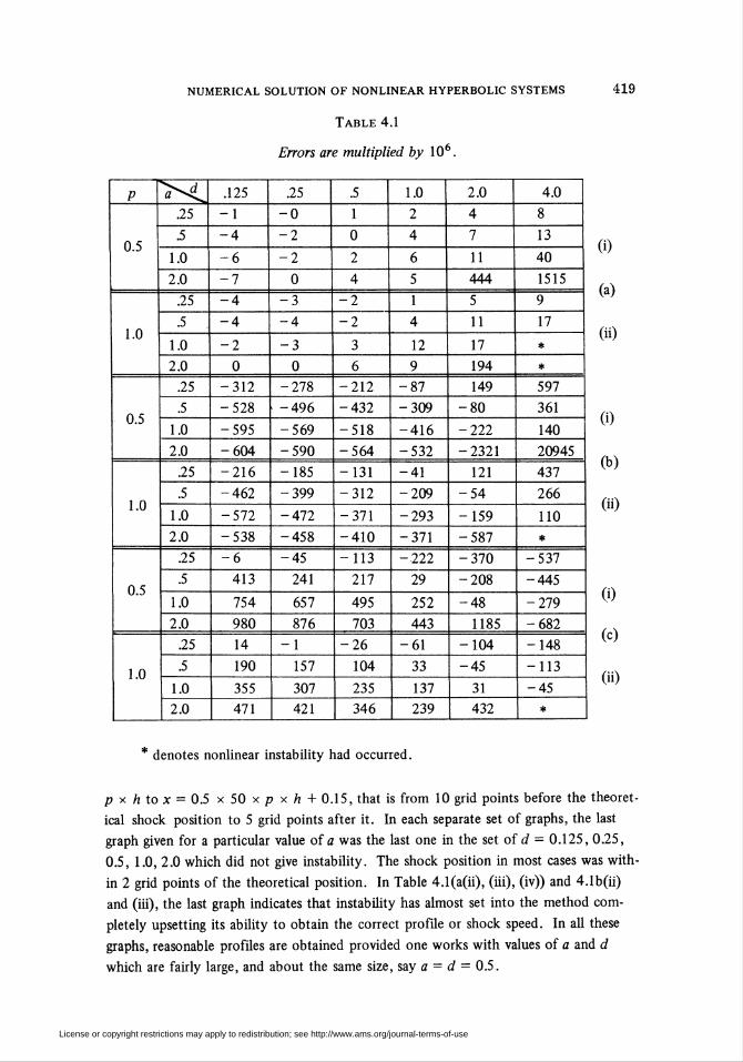
Table 4.1

Errors are multiplied by 106.

.25

1.0

2.0

.25

1.0

2.0

.25

1.0

2.0

.125

312-528

-595

-604

.25

1.0

2.0

.25

.5

1.0

2.0

.25

1.0

2.0

216■462

-572

-538

-6

413

754

980

14

190

355

471

.25-0

-2

-3

■278

-496

-569

.5

212-432

-590

-185

-399

■472

•458

-45

241

657

876

157

307

421

518-564

1.0

12

■87

-309

■416

•532

2.0

11

444

11

17

194

149-80

222

2321-131

-312

371•410

-113

217

495

703

26

104

235

346

-41

-209

-293

-371

222

29

252

443

61

33

137

239

121-54

-159

-587

-370

-208

-48

1185-104

-45

31

432

4.0

13

40

1515

17

597

361

140

20945

437

266

110

537-445

-279

-682

148

113■45

419

(i)

(a)

(Ü)

(i)

(b)

Oi)

0)

(c)

(Ü)

denotes nonlinear instability had occurred.

p x ft to x = 0.5 x 50 x p x ft + 0.15, that is from 10 grid points before the theoret-

ical shock position to 5 grid points after it. In each separate set of graphs, the last

graph given for a particular value of a was the last one in the set of d = 0.125, 0.25,

0.5, 1.0, 2.0 which did not give instability. The shock position in most cases was with-

in 2 grid points of the theoretical position. In Table 4.1(a(ii), (iii), (iv)) and 4.1b(ii)

and (iii), the last graph indicates that instability has almost set into the method com-

pletely upsetting its ability to obtain the correct profile or shock speed. In all these

graphs, reasonable profiles are obtained provided one works with values of a and d

which are fairly large, and about the same size, say a = d = 0.5.



Figure 4.1

k (a) p = 0-95

(i) a = 0-5

.d = 012E d = Q-2S d = 0»5 d = 1-0

(ii) a = 1-0

(iii) a = 2«0

d « 0•12 S d = 0-25 d = 0-5'

(iv) a = H'O

d = 0-125 Id = 0-25;

From these results, it is desirable to work with a value of p close to the stability

limit and to choose ad inside the range predicted by Theorem 4.5. Further, in the ab-

sence of any other criteria, one could choose ad so as to satisfy the stability criteria of

the implicit scheme itself, namely (3.6), and a so as to centralise the scheme, that is

take a around 0.5.


NUMERICAL SOLUTION OF NONLINEAR HYPERBOLIC SYSTEMS

Figure 4.{(continued)

421

(b) p = 0-5

(i) a = 1-0

d = 0-125 d = 0-5

-A

d = 1-0 d = 2-0

(ii) a = 2-0

d = 0-125 d = 0-5 d = 1-0 d = 2-0

(iii) a = 4-0

d = 0-25 d = 0-5 d = 1-0

These results simply represent a preliminary study of this type of explicit-implicit

method. Applications to more complicated equations and systems arising from physi-

cal problems will be carried out in the near future.

5. Extension of Explicit-Implicit Schemes to Two Space Dimensions. In this sec-

tion, the extension of the explicit-implicit ideas of Section 2 are carried through to



problems involving two space dimensions. We consider the system of conservation laws

(5.1) bu/bt + bf(u)lbx + bg(u)lby = 0

in a region R x (0, °°) where R is a bounded region of (x, j>)-space. Appropriate initial

and boundary conditions are asumed given.

A grid of spacing h and a time step k is placed on R and the time axis, respec-

tively. wH1 denotes an approximation to u(ih, jh, mk).

In a manner analogous to that in Richtmyer's paper [3], the explicit and implicit

schemes can be extended to solve (5.1) (see [5], [11]). We denote by

(5.2) w^ + 1=Äew,7

the two-dimensional analogue of the explicit scheme and by

(5.3) RoiK + l=R"<

the two-dimensional analogue of the implicit scheme. The operators Re, R0I, RXI are

nonlinear operators. R0Iw™ + i involves values of wm + l at (i, j), (i ± 1,/), (/, / ± 1).

We now consider different combinations of the schemes (5.2), (5.3) in a similar

way to that described for parabolic problems in Gourlay and McGuire [14] and McGuire

[15]. An Odd-Even explicit-implicit method (see [14]) may be defined by the following

strategy:use (5.2) at those points with m + i + j odd,

(5 4)v ' ' and use (5.3) at the points with m + i + j even.

This method used progressively from time level to time level is easily seen to be com-

pletely explicit. For, after appliction of (5.2) at all points on time level m + 1 with

m + i +/ odd, the only unknown in the expression R0jW^+l when (5.3) is applied at

the points with m + i + j even, is in fact w™ +1.

In a similar way, a line explicit-implicit method may be defined by the procedure:

use (5.2) at those points with m + i odd,

and use (5.3) at those with m + i even.

This method is not completely explicit, and requires the solution of a nonlinear block

tridiagonal system on alternate i grid lines at each time level. Methods similar to those

for implementing the implicit schemes in one space dimension (see [11]) are required

to solve these systems.

Also an alternating direction explicit-implicit method may be defined by the al-

gorithm:

on odd time levels, use (5.2) at points with m + i even

and then use (5.3) at points with m + i odd;

^ * ' on even time levels use (5.2) at points with m + / even

and then (5.3) at points with m + j odd.

This method is seen to be partially implicit requiring the solution of a nonlinear block

tridiagonal system on alternate i grid lines for odd time levels and the solution of a

nonlinear block tridiagonal system on alternate / grid lines for even time levels.

Other combinations are possible. The analysis of the stability properties of the

methods like (5.4), (5.5), (5.6) is complicated. Each of the methods, when linearized,



can be reduced to a three-level method on explicit node points only. The amplifica-

tion matrix can then be investigated in the same way as for the one-space dimensional case.

The explicit-implicit schemes of Section 2 can also be extended using Strang's for-

mulations [21], [22] or the formulation in McGuire and Morris [23]. However, the in-

vestigation of the linearized stability properties of the resulting methods is difficult since

each one space dimensional operator is a three-level operator and thus the usual tech-

nique (see [21], [22]) of finding the amplification matrix cannot be applied directly.

No experiments have been carried out with any of the above methods as yet; it is

hoped to conduct investigations of this type in the near future.

Department of Mathematics

Heriot-Watt University

Riccarton, Currie, Edinburgh, Scotland

Department of Mathematics

University of Dundee

Dundee, Scotland

1. A. JEFFREY & T. TANUITI, Non-Linear Wave Propagation with Applications to Physics

and Magnetohydrodynamics, Academic Press, New York and London, 1964. MR 29 #4410.

2. O. A. OLEINIK, "On discontinuous solutions of non-linear differential equations," Dokl.

Akad. Nauk SSSR, v. 109, 1956, pp. 1098-1101. (Russian) MR 18, 656.

3. R. D. RICHTMYER, A Survey of Difference Methods for Non-Steady Fluid Dynamics,

NCAR Technical Notes 63-2, 1962.

4. A. R. GOURLAY & J. LI. MORRIS, "Finite-difference methods for nonlinear hyperbolic

systems," Math. Comp., v. 22, 1968, pp. 28-39. MR 36 #6163.

5. G. R. MCGUIRE & J. LI. MORRIS, " A class of second order accurate methos for the so-

lution of systems of conservation laws," J. Computational Phys., v. 11, 1973, pp. 531—549.

6. P. D. LAX & B. WENDROFF, "Systems of conservation laws," Comm. Pure Appl. Math.,

v. 13, 1960, pp. 217-237. MR 22 #11523.

7. P. D. LAX, "Weak solutions on nonlinear hyperbolic equations and their numerical com-

putation," Comm. Pure Appl. Math., v. 7, 1954, pp. 159-193. MR 16, 524.

8. R. D. RICHTMYER & K. W. MORTON , Difference Methods for Initial-Value Problems,

2nd ed., Interscience Tracts in Pure and Appl. Math., no. 4, Interscience-Wiley, New York, 1967.

MR 36 #3515.9. R. COURANT, K. O. FRIEDRICHS & M. LEWY, "On the partial difference equations of

mathematical physics'" IBM J. Res. Develop., v. 11, 1967, pp. 215-234. MR 35 #4621.

10. J. GARY, "On certain finite difference schemes for hyperbolic systems," Math. Comp.,

V. 18, 1964, pp. 1-18. MR 28 #1776.11. G. R. MCGUIRE & J. LI. MORRIS, "A class of implicit, second order accurate dissipa-

tive schemes for solving systems of conservation laws," /. Computational Phys., v. 14, 1974, pp.

126-147.12. S. ABARBANEL & G. ZWAS, "An iterative finite-difference method for hyperbolic sys-

tems," Math. Comp., v. 23, 1969, pp. 549-565. MR 40 #1044.13. A. R. GOURLAY, "Hopscotch: A fast second-order partial differential equation solver,"

/. Inst. Math. Appl., v. 6, 1970, pp. 375-390. MR 43 #4267.14. A. R. GOURLAY & G. R. MCGUIRE, "General hopscotch algorithm for the numerical

solution of partial differential equations," J. Inst. Math. Appl., v. 7, 1971, pp. 216-227. MR 44

#4929.15. PAUL GORDON, "Nonsymmetric difference equations,"/. Soc. Indust. Appl. Math.,

v. 13, 1965, pp. 667-673. MR 32 #3290.16. S. M. SCALA &. P. GORDON, "Solution of the time-dependent Navier-Stokes equations

for the flow around a circular cylinder," AIAA J., v. 6, 1968, pp. 815-822.17. A. R. GOURLAY & J. LI. MORRIS, "Hopscotch difference methods for nonlinear hy-

perbolic systems," IBM J. Res. Develop., v. 16, 1972, pp. 349-353.



18. A. R. GOURLAY, G. R. MCGUIRE & J. LI. MORRIS, One Dimensional Methods for

the Numerical Solution of Nonlinear Hyperbolic Equations, IBM UK Rep. #12, 1972.

19. JOHN J. H. MILLER, "On the location of zeros of certain classes of polynomials with

applications to numerical analysis," /. Inst. Math. Appl, v. 8, 1971, pp. 397-406. MR 45 #9481.

20. G. R. MCGUIRE, Hopscotch Methods for the Solution of Linear Second Order Parabolic

Partial Differential Equations, M. Sc. Thesis, University of Dundee, 1970.

21. GILBERT STRANG, "Accurate partial difference methods. II. Non-linear problems,"

Numer. Math., v. 6, 1964, pp. 37-46. MR 29 #4215.

22. GILBERT STRANG, "On the construction and comparison of difference schemes," SIAM

J. Numer. Anal, v. 5, 1968, pp. 506-517. MR 38 #4057.

23. G. R. MCGUIRE & J. LI. MORRIS, "Restoring orders of accuracy for multilevel schemes

for nonlinear hyperbolic systems in many space variables." (To appear.)

24. E. L. RUBIN & S. Z. BURSTEIN, "Difference methods for the inviscid and viscous equa-

tions of a compressible gas," /. Computational Phys., v. 2, 1967, pp. 178—196.

25. P. J. ROACHE, Computational Fluid Dynamics, Hermosa, Albuquerque, N. M., 1972.


Documents

Explicit-Implicit Schemes for the Numerical Solution of ... increased stability range for the implicit schemes are unfortunately offset by two important disadvantages. First, the implicit