Embed Size (px)
Citation preview

Wolf-Jurgen BeynRaphael Kruse
Numerical Methods for StochasticProcesses
– Vorlesungsskript –Universitat BielefeldSommersemester 2011
August 26, 2011


Preface
These lecture notes grew out of a courseNumerical Methods for Stochastic Pro-cessesthat the authors taught at Bielefeld University during the summer term2011. The text contains material for about 30 two-hour lectures and includes a se-ries of exercises most of which were assigned during the course. We assume thatreaders/participants have a firm basis in measure theory andprobability theory asusually provided during a one-semester course. To a lesser extent experience withbasic numerical methods from a one-semester course is also very helpful.
The lecture notes adress Bachelor students in their third year and Master stu-dents in their first year. For Bachelor students the topics maybe taken as a basisfor writing a Bachelor Thesis while for Master students they may serve as a start-ing point for a specialization in numerical methods for stochastic ordinary andpartial differential equations.
v


Contents
1 Introduction . . . . . . . . . . . . . . . . . . . . . . . . . . . . . . . . . . . . . . . . . . . . . . . . . 11.1 Financial Options . . . . . . . . . . . . . . . . . . . . . . . . . . . . . . . .. . . . . . . . . . 11.2 Asset Price Model . . . . . . . . . . . . . . . . . . . . . . . . . . . . . . . . .. . . . . . . . 31.3 Black-Scholes Formula . . . . . . . . . . . . . . . . . . . . . . . . . . . . .. . . . . . . . 81.4 Monte Carlo Methods for Financial Option Valuation . . . . .. . . . . . . 10
2 Preliminaries from Probability Theory . . . . . . . . . . . . . . . . . . . . . . . . . . 152.1 Probability Spaces and Random Variables . . . . . . . . . . . . . .. . . . . . . 152.2 Independence and Distributions of Random Variables . . . .. . . . . . . . 172.3 Integrability and Moments of Random Variables . . . . . . . . .. . . . . . . 192.4 The Transformation Theorem for Integrals . . . . . . . . . . . .. . . . . . . . . 232.5 Some Standard Distributions . . . . . . . . . . . . . . . . . . . . . . .. . . . . . . . . . 242.6 Conditional Expectations . . . . . . . . . . . . . . . . . . . . . . . . . .. . . . . . . . . . 252.7 Limit Theorems . . . . . . . . . . . . . . . . . . . . . . . . . . . . . . . . . . .. . . . . . . . 27
3 Generating Random Numbers. . . . . . . . . . . . . . . . . . . . . . . . . . . . . . . . . . 333.1 Motivation . . . . . . . . . . . . . . . . . . . . . . . . . . . . . . . . . . . . . .. . . . . . . . . . 333.2 Pseudo-Random Number Generators . . . . . . . . . . . . . . . . . . . .. . . . . . 343.3 Linear Congruential Generators . . . . . . . . . . . . . . . . . . . . .. . . . . . . . . 373.4 Empirical Tests . . . . . . . . . . . . . . . . . . . . . . . . . . . . . . . . . .. . . . . . . . . . 403.5 The Mersenne Twister . . . . . . . . . . . . . . . . . . . . . . . . . . . . . .. . . . . . . . 45
4 Generating Random Variables with Non-Uniform Distributi on . . . . . 494.1 Inversion Method . . . . . . . . . . . . . . . . . . . . . . . . . . . . . . . . .. . . . . . . . . 494.2 Rejection Method . . . . . . . . . . . . . . . . . . . . . . . . . . . . . . . . . .. . . . . . . . 504.3 The Box-Muller Method . . . . . . . . . . . . . . . . . . . . . . . . . . . . . .. . . . . . 534.4 Marsaglia’s Ziggurat Method . . . . . . . . . . . . . . . . . . . . . . .. . . . . . . . . 55
vii
viii Contents
5 Monte Carlo Methods . . . . . . . . . . . . . . . . . . . . . . . . . . . . . . . . . . . . . . . . . 615.1 Statistical Analysis of Simulation Output . . . . . . . . . . .. . . . . . . . . . . 615.2 Monte Carlo Integration . . . . . . . . . . . . . . . . . . . . . . . . . . . .. . . . . . . . 655.3 Variance Reduction Techniques . . . . . . . . . . . . . . . . . . . . . .. . . . . . . . 675.4 Approximation of Multiple Integrals . . . . . . . . . . . . . . . .. . . . . . . . . . 78
6 Theory of Continuous Time Stochastic Processes and Ito-Integrals . 876.1 Continuous Time Stochastic Processes . . . . . . . . . . . . . . . .. . . . . . . . 876.2 Martingales . . . . . . . . . . . . . . . . . . . . . . . . . . . . . . . . . . . . .. . . . . . . . . . 906.3 Brownian Motion . . . . . . . . . . . . . . . . . . . . . . . . . . . . . . . . . . .. . . . . . . 936.4 The Ito-Integral . . . . . . . . . . . . . . . . . . . . . . . . . . . . . . . . . . . . . . . . .. . . 1036.5 Ito’s Formula . . . . . . . . . . . . . . . . . . . . . . . . . . . . . . . . . . . . . . . . .. . . . . 114
7 Stochastic Ordinary Differential Equations . . . . . . . . . . . . . . . . . . . . . . 117
8 Numerical Solution of SODEs. . . . . . . . . . . . . . . . . . . . . . . . . . . . . . . . . . 119
9 Weak Approximation of SODEs . . . . . . . . . . . . . . . . . . . . . . . . . . . . . . . . 121
10 Monte Carlo Methods for SODEs. . . . . . . . . . . . . . . . . . . . . . . . . . . . . . . 123
References. . . . . . . . . . . . . . . . . . . . . . . . . . . . . . . . . . . . . . . . . . . . . . . . . . .. . . . 125
Index . . . . . . . . . . . . . . . . . . . . . . . . . . . . . . . . . . . . . . . . . . . . . . . . . . .. . . . . . . . 129
Symbols and Acronyms
/0 the empty setΩ set of elementary eventsAc complementΩ \A of a subsetA⊂ Ω1A indicator function of the setA see (2.2)R set of real numbersRd vector space ofd-dimensional tuples(x1, . . . ,xd) with xi ∈ R, i = 1, . . . ,dRm,d vector space of realm×d-matricesB(Rd) Borel-σ -algebra onRd
M interior of a subsetM ⊂ Rd
λ d Lebesgue measure onRd
|x| absolute value ofx if x∈ R or Euclidean norm ofx if x∈ Rd
M2([0,T]) Banach space of continuous, square-integrable,Rm-valued (Ft)-martingales (also written asM2([0,T];Rm))
Vba (X) bounded variation of a stochastic processX on [a,b], see (6.5)
〈X〉[a,b] quadratic variation of a stochastic processX on [a,b], see (6.6)
a.e. almost everywhere, synonymous with a.s.a.s. almost surely, or with probability 1i.i.d. independent and identically distributedc.d.f. cumulative distribution functionCLT central limit theoremp.d.f. probability density functionLCG linear congruential generatorLLN law of large numbersODE ordinary differential equationPDE partial differential equationPRNG pseudo-random number generatorSODE stochastic ordinary differential equation
ix

Chapter 1Introduction
In this chapter we present the basic ideas of the option valuation theory as a moti-vating example. Mathematical finance, and the Black-Scholesmodel in particular,is easily accessible and provides a range of typical and non-trivial applications ofthe different numerical methods which we will discuss later.
Here, we give an overview of the standard Black-Scholes model. At someplaces we already use terminology which will be introduced in later chapters. Onfirst reading we recommend that the reader simply skip over unknown technicalterms.
The content of this chapter is based on [12, 13, 14, 22, 32].
1.1 Financial Options
A financial derivative is a contract which value depends on the expected pricemovement of an underlyingasset. An asset is anything tangible or intangiblewhich can be owned and traded for cash. For example, this includes commodi-ties such as oil or gold, as well as shares or bonds which are traded on the stockmarket.
In this chapter we are interested in a very specific financial derivative, the socalled European call option, which we define in the same way asin [14].
Definition 1.1.A European call optiongives itsholder the right (but not the obli-gation) to purchase from thewriter a prescribed assetS (the underlying) for aprescribed priceE > 0 (theexercise price) at a prescribed timeT > 0 (theexpirydate) in the future.
For example, I (the writer) may offer you (the holder) the right to buy a shareof the Apple Inc. (the underlying) for 300 USD (the exercise price) three monthsfrom now (expiry date). In three months there are two possible scenarios:
1

2 1 Introduction
0 100 200 300 400 500 600asset price S at expiry
0
50
100
150
200
250
300
payoff
Payoff of a European call option
Fig. 1.1 The payoff diagram of the European call option withE = 300.
a) The market price of the Apple Inc. share is higher than 300 USD. Then itmakes sense for you to exercise the option and, if you immediately sell theshare, you will gain the positive difference between the exercise price and themarket price.
b) If the market price is lower than 300 USD then you simply letthe optionexpire and you may buy the share on the open stock market for the lowerprice.
In none of the scenarios, as it is indicated in Figure 1.1, youare loosing moneybut in case a) your gain is potentially unlimited. For me as the holder, however, Iam facing a loss in scenario a) and no gain in b). So, in exchange for the option Imay ask you for a compensation.
This chapter is devoted to answer the question how do we determine afair valueof this option. But before we follow in the footprints of the Nobel prize winningpaper by Black and Scholes [6] let us briefly note why this question is important.
On the financial markets options and other derivatives, suchas swaps and fu-tures, have become increasingly popular. In some cases moremoney is invested

1.2 Asset Price Model 3
in the derivatives than in the underlying asset. The two mostcommon motivationsfor investors to buy options arehedgingandspeculations.
Investors, who buy options in order to hedge a risk, use them in the same way asan insurance police. For example, consider an European investor who is planningto buy a factory in the USA which costs 10 million USD. The amount of moneyis payable in three months. If the investor is worried about adevaluation of thecurrency rate of the Euro he may consider to buy an options which gives him theright to buy 10 million USD for a fixed exchange rate in three month. Thus, theexercise price can be interpreted as a worst-case scenario.
On the other hand, investors may also buy options to speculate on price move-ments of the underlying assets. If the price of the underlying climbs by one per-cent the value of a corresponding European call usually climbs by a much largeramount. Therefore, the investor makes a larger profit by investing the same amountof money in the option instead of directly buying the underlying asset. Of course,the same holds true for possible losses if the price of the underlying asset movesin the wrong direction.
1.2 Asset Price Model
In this section we formulate our assumptions and derive a mathematical model forthe price movements of the underlying asset.
Assumption 1.2 (Bank account).We postulate the existence of a risk-free bankaccount with continuously compoundedinterest rate r≥ 0. We are allowed todeposit or borrow any arbitrary amount of money at any time. The interest rate isassumed to be constant. ByB(t) we denote the balance of the bank account.
In practice, Assumption 1.2 is not satisfied for several reasons: The interestrate is usually not fixed and banks often charge a higher interest rate on creditsthan they pay on saving accounts. However, we interpret our assumption as anapproximation of the reality on short time intervals.
If we put an amount ofB0 on the account at timet0 then, at timet1 > t0, wehave
B(t1) = er(t1−t0)B0. (1.1)
Therefore, the balance processB(t) follows the linear ordinary differential equa-tion
ddt
B(t) = rB(t), B(t0) = B0. (1.2)

4 1 Introduction
0 2 4 6 8 10time t
1.0
1.1
1.2
1.3
1.4
1.5
1.6
1.7balance
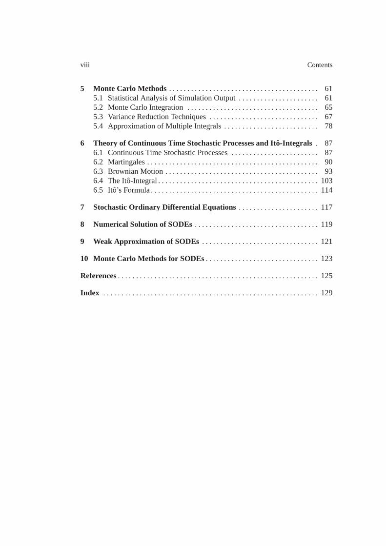
Balance of a bank account, r=0.05
Fig. 1.2 Balance of a bank account with fixed continuously compounded interest rater = 0.05 and initial capital of 1 euro. The scale of the time axis is measured in years.
A typical value of the parameterr is 0.05 which corresponds to an interest rate of5% per year. Figure 1.2 illustrates the development of the balanceB(t) over tenyears.
A consequence of our assumption is that two offers of
a) 100 euros at timet = 0, orb) ert 100 euros at timet > 0
can be considered to be equal. In fact, by borrowing or investing the money bothoffers can be transformed into the other.
In a similar way, 100 euros at timet > 0 are worth 100e−rt euros at time zero.This concept is calleddiscounting for interestor discounting for inflation.
The following assumption provides a structural framework for our financialmarket.
Assumption 1.3.a) In addition to the bank account our financial market onlyconsists of one risky asset. ByS(t) we denote the nonnegative value of oneunit of the risky asset at time 0≤ t ≤ T.
1.2 Asset Price Model 5
b) It is possible to buy and sell any real number of units of theasset at the marketpriceS(t) at any time 0≤ t ≤ T.
c) There are no transaction costs and the asset is paying no dividends.d) Short selling is allowed, that is, it is possible to hold a negative amount of the
asset.
The theory of Black and Scholes also builds on the following fundamental as-sumption which states the absence ofarbitrages. Although there exists a rigorousdefinition of an arbitrage we follow [14] and only provide a verbal formulation ofthe idea.
Assumption 1.4.There is never an opportunity to make a risk-free profit that givesa greater return than that provided by the interest from the bank account.
For a moment, assume that Assumption 1.4 is violated and there exists an ar-bitrage opportunity, then investors would simply borrow cash from the bank andtake advantage of the arbitrage on a large scale. By the forcesof supply and de-mand this would affect the market prices or interest rates until the opportunity hasvanished. Therefore, in practice, if arbitrage opportunities exist in an efficient andliquid financial market then they should be short lived.
After setting a framework of our financial market we introduce a model for theasset price movements. Which properties should we demand from this model?First of all, sinceS(t) describes the evolution of a price process it is reasonableto forceS(t) to be nonnegative. Further, since the assetS represents the erraticdynamics of stock prices,S should statistically behave in a similar way as realstock market data. This leads to the idea to modelSas a stochastic process.
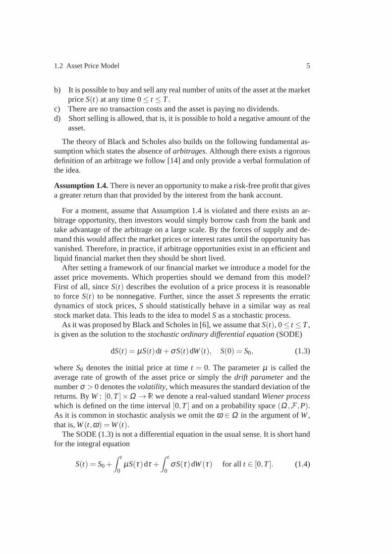
As it was proposed by Black and Scholes in [6], we assume thatS(t), 0≤ t ≤ T,is given as the solution to thestochastic ordinary differential equation(SODE)
dS(t) = µS(t)dt +σS(t)dW(t), S(0) = S0, (1.3)
whereS0 denotes the initial price at timet = 0. The parameterµ is called theaverage rate of growth of the asset price or simply thedrift parameterand thenumberσ > 0 denotes thevolatility, which measures the standard deviation of thereturns. ByW : [0,T]×Ω → R we denote a real-valued standardWiener processwhich is defined on the time interval[0,T] and on a probability space(Ω ,F ,P).As it is common in stochastic analysis we omit theω ∈ Ω in the argument ofW,that is,W(t,ω) =W(t).
The SODE (1.3) is not a differential equation in the usual sense. It is short handfor the integral equation
S(t) = S0+∫ t
0µS(τ)dτ +
∫ t
0σS(τ)dW(τ) for all t ∈ [0,T]. (1.4)

6 1 Introduction
0 2 4 6 8 10t
0.9
1.0
1.1
1.2
1.3
1.4
1.5
1.6
1.7S(t)
Asset price trajectories
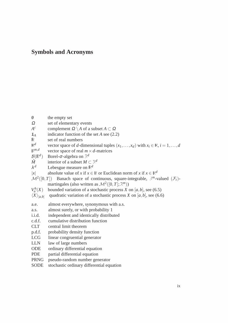
Fig. 1.3 Two typical realizations of the stochastic asset price process (1.5) with parametervaluesT = 10,S0 = 1, µ = 0.05, andσ = 0.2.
While the first integral is a well-known Lebesgue or Riemann-integral, the secondintegral is a so called stochastic Ito-integral, named after Kiyoshi Ito. The solutionprocessS: [0,T]×Ω → R to (1.3) is explicitly given by
S(t) = S0e(µ−12σ2)t+σW(t). (1.5)
Without using any knowledge on the Wiener processW(t) we derive from (1.5)thatS(t) is in fact nonnegative.
For ω ∈ Ω we call the mappingt 7→ S(t,ω) a sample pathof the stochasticprocessS. Figure 1.3 shows two typical sample paths of the asset pricemodel(1.5).
For the definition ofSwe used terminology from stochastic analysis which wedid not explain so far. This will be done in full detail in Chapter 6. For the rest ofthis section we aim to facilitate an intuitive understanding of the solution to (1.3).
Let 0≤ t0 < t1 ≤ T be arbitrary. Then by (1.4) we have
1.2 Asset Price Model 7
S(t1)−S(t0) =∫ t1
t0µS(τ)dτ +
∫ t1
t0σS(τ)dW(τ).
Next, under the assumption that the time lengtht1− t0 is sufficiently small, weapproximate both integrals by
∫ t1
t0µS(τ)dτ +
∫ t1
t0σS(τ)dW(τ)≈ µS(t0)(t1− t0)+σS(t0)
(
W(t1)−W(t2))
.
By using this we get
S(t1)−S(t0)S(t0)
≈ µ(t1− t0)+σ(
W(t1)−W(t2))
. (1.6)
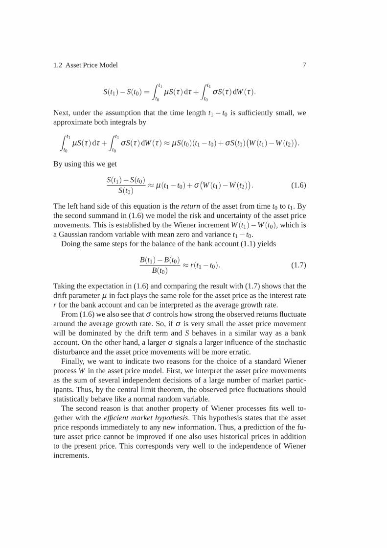
The left hand side of this equation is thereturn of the asset from timet0 to t1. Bythe second summand in (1.6) we model the risk and uncertaintyof the asset pricemovements. This is established by the Wiener incrementW(t1)−W(t0), which isa Gaussian random variable with mean zero and variancet1− t0.
Doing the same steps for the balance of the bank account (1.1)yields
B(t1)−B(t0)B(t0)
≈ r(t1− t0). (1.7)
Taking the expectation in (1.6) and comparing the result with (1.7) shows that thedrift parameterµ in fact plays the same role for the asset price as the interestrater for the bank account and can be interpreted as the average growth rate.
From (1.6) we also see thatσ controls how strong the observed returns fluctuatearound the average growth rate. So, ifσ is very small the asset price movementwill be dominated by the drift term andS behaves in a similar way as a bankaccount. On the other hand, a largerσ signals a larger influence of the stochasticdisturbance and the asset price movements will be more erratic.
Finally, we want to indicate two reasons for the choice of a standard WienerprocessW in the asset price model. First, we interpret the asset pricemovementsas the sum of several independent decisions of a large numberof market partic-ipants. Thus, by the central limit theorem, the observed price fluctuations shouldstatistically behave like a normal random variable.
The second reason is that another property of Wiener processes fits well to-gether with theefficient market hypothesis. This hypothesis states that the assetprice responds immediately to any new information. Thus, a prediction of the fu-ture asset price cannot be improved if one also uses historical prices in additionto the present price. This corresponds very well to the independence of Wienerincrements.

8 1 Introduction
Remark 1.5.In practice, the asset price model (1.3) only gives useful approxima-tions of the reality on very short time scales. Since the publication of the Black-Scholes formula in [6] more advanced asset price models havebeen developed.As a starting point we refer to [11].
1.3 Black-Scholes Formula
In this section we determine a mappingC: [0,T]×R+ → R+ such thatC(t,s)denotes the fair value of a European call at timet, if the call option expires at timeT and the price of the underlying asset at timet is S(t) = s.
Further, byE > 0 we denote the exercise price. Then, by Definition 1.1, wealready know that
C(T,s) = max(0,s−E). (1.8)
Under the asset price model and assumptions from Section 1.2Black and Scholes[6] proved that the mappingC is the solution to the partial differential equation(PDE)
∂C(t,s)∂ t
+12
σ2s2∂ 2C(t,s)∂s2 + rs
∂C(t,s)∂s
− rC(t,s) = 0. (1.9)
This is the so calledBlack-Scholes PDE. In Chapter 6 we will present a derivationof this equation when we have the Ito formula at our disposal.
Together with the final time condition (1.8) there exists a unique solution tothe Black-Scholes PDE. Moreover, Black and Scholes also presented an explicitrepresentation of the solution, the famousBlack-Scholes formulafor Europeancall options.
Theorem 1.6 (Black-Scholes formula for European call options). There existsa unique solution C: [0,T]×R+ → R+ to the Black-Scholes PDE(1.9) whichsatisfies the final time condition(1.8). The solution is explicitly given by
C(t,s) = sFN(0,1)(d1)−Ee−r(T−t)FN(0,1)(d2), (1.10)
where FN(0,1) is the cumulative probability distribution of the standardnormaldistribution, that is
FN(0,1)(x) =1√2π
∫ x
−∞e−
12z2
dz.
In addition, d1 and d2 are given by
1.3 Black-Scholes Formula 9
t
0.00.2
0.40.6
0.81.0
s
0.6
0.8
1.0
1.21.4
C(t,s)
0.0
0.1
0.2
0.3
0.4
0.5
t
0.00.2
0.40.6
0.81.0
s
0.6
0.8
1.0
1.21.4
C(t,s)
0.0
0.1
0.2
0.3
0.4
0.5
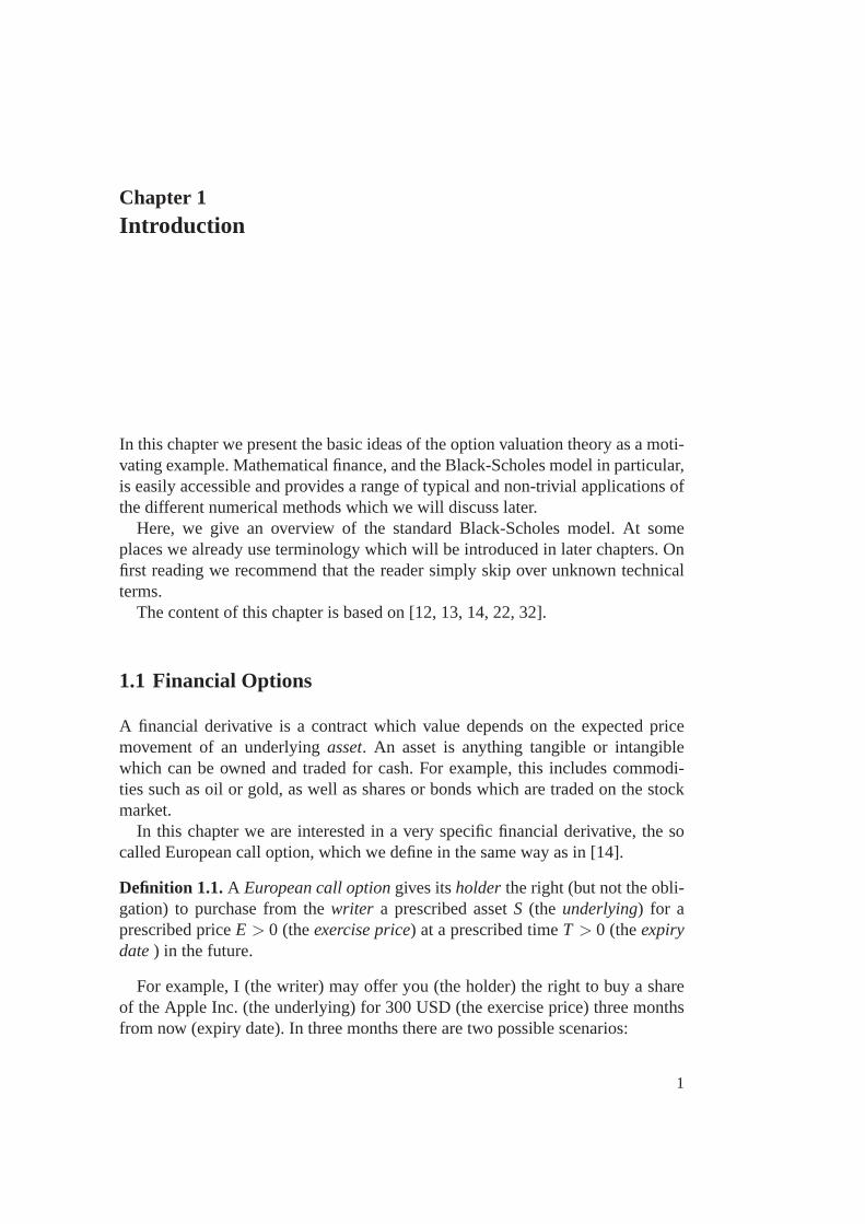
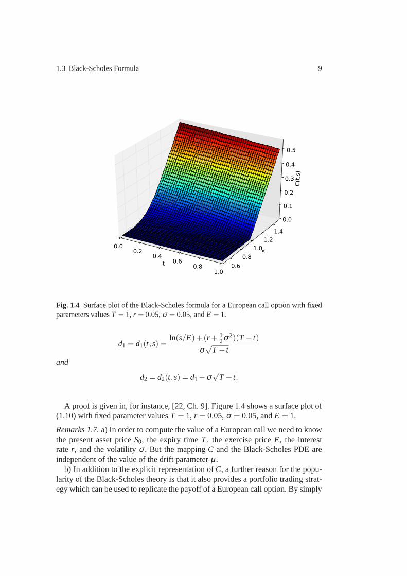
Fig. 1.4 Surface plot of the Black-Scholes formula for a European call option withfixedparameters valuesT = 1, r = 0.05,σ = 0.05, andE = 1.
d1 = d1(t,s) =ln(s/E)+(r + 1
2σ2)(T − t)
σ√
T − t
and
d2 = d2(t,s) = d1−σ√
T − t.
A proof is given in, for instance, [22, Ch. 9]. Figure 1.4 showsa surface plot of(1.10) with fixed parameter valuesT = 1, r = 0.05,σ = 0.05, andE = 1.
Remarks 1.7.a) In order to compute the value of a European call we need to knowthe present asset priceS0, the expiry timeT, the exercise priceE, the interestrate r, and the volatilityσ . But the mappingC and the Black-Scholes PDE areindependent of the value of the drift parameterµ.
b) In addition to the explicit representation ofC, a further reason for the popu-larity of the Black-Scholes theory is that it also provides a portfolio trading strat-egy which can be used to replicate the payoff of a European call option. By simply

10 1 Introduction
following this hedgingstrategy a bank can sell options without taking risks. Forfurther reading we refer to [14].
1.4 Monte Carlo Methods for Financial Option Valuation
The Black-Scholes formula (1.10) gives an analytic solutionto the problem ofdetermining the fair value of a European call option. Therefore, we could considerthe problem as being solved. However, as it is pointed out by D. Higham [13, 14],there are many variations of the option valuation problem, where a simple analyticsolution does not exist.
For instance, this is true for so called exotic options [14],where the payoff notonly depends on the final time asset price, but also on its behaviour during thetime interval[0,T]. The same problem occurs when we invoke a different assetprice model. For example, we refer to [22, Ch. 9.2] for severalvariations.
The aim of this section and, in fact, of the whole lecture is topresent and an-alyze numerical methods for applications where analytic solutions are not avail-able. Here, we focus onMonte Carlo methods. Roughly speaking, a Monte Carlomethod tries to approximate the mean of a random variableX by the average overa large numberN of independent outcomes ofX, that is
E[X]≈ 1N
N
∑i=1
X(ωi) for N large.
In the context of the option valuation problem, other numerical approaches containnumerical approximation of the solution to the Black-Scholes PDE (1.9) or theuse of simplified asset price models, for example, the binomial method. For theseapproaches, we refer to [14, 12].
In the following we will again discuss the problem of the valuation of a Euro-pean call option under the conditions of Section 1.2. The basic idea, how to applya Monte Carlo method, is to use thediscounted expected payoffas the optionprice, that is, the value is given by
V(S0) =V(S0; µ,σ ,T,E, r) = e−rT E[
max(0,S(T)−E)]
, (1.11)
where, as above,S0 is the present price of the asset,T andE denote the expirydate and exercise price of the option, andr is the riskless interest rate. The assetpriceS(T) is given by the SODE (1.3) with drift parameterµ and volatilityσ > 0.
This approach leads to two questions:
a) What is the relationship between the discounted expected payoff V and theBlack-Scholes formula (1.10)?
1.4 Monte Carlo Methods for Financial Option Valuation 11
0.00 0.01 0.02 0.03 0.04 0.05 0.06 0.07 0.08 0.09 0.10µ
0.8
0.9
1.0
1.1
1.2
1.3
1.4
1.5
Discounted expected payoff
dis. expected payoffBlack-Scholes price
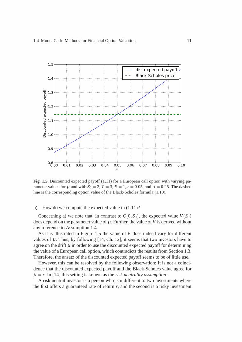
Fig. 1.5 Discounted expected payoff (1.11) for a European call option with varying pa-rameter values forµ and withS0 = 2, T = 3, E = 1, r = 0.05, andσ = 0.25. The dashedline is the corresponding option value of the Black-Scholes formula (1.10).
b) How do we compute the expected value in (1.11)?
Concerning a) we note that, in contrast toC(0,S0), the expected valueV(S0)does depend on the parameter value ofµ. Further, the value ofV is derived withoutany reference to Assumption 1.4.
As it is illustrated in Figure 1.5 the value ofV does indeed vary for differentvalues ofµ. Thus, by following [14, Ch. 12], it seems that two investors have toagree on the driftµ in order to use the discounted expected payoff for determiningthe value of a European call option, which contradicts the results from Section 1.3.Therefore, the ansatz of the discounted expected payoff seems to be of little use.
However, this can be resolved by the following observation:It is not a coinci-dence that the discounted expected payoff and the Black-Scholes value agree forµ = r. In [14] this setting is known as therisk neutrality assumption.
A risk neutral investor is a person who is indifferent to two investments wherethe first offers a guaranteed rate of returnr, and the second is a risky investment
12 1 Introduction
with same expected rate of returnr (Usually, investors are assumed to be risk-averse, which means that they will prefer the first investment).
In the caseµ = r one can show thatE[S(t)] = S0ert which coincides with thebalance process of the bank account (1.1). Thus, risk neutral investors have nopreferences between investing in the bank account and in therisky assetS.
Without going into details, it is possible to transform the underlying measurePinto a measureP in such a way that investors behave risk neutral with respectto P.This is achieved by an application of Girsanov’s Theorem [22, Ch. 8, Th. 2.2] andleads to the so called martingale approach to option valuation. For further readingwe refer to [15].
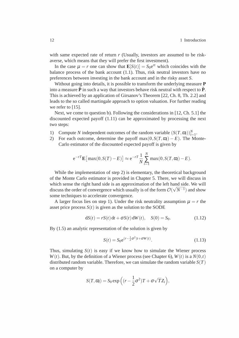
Next, we come to question b). Following the considerations in [12, Ch. 5.1] thediscounted expected payoff (1.11) can be approximated by processing the nexttwo steps:
1) ComputeN independent outcomes of the random variable(S(T,ωi))Ni=1.
2) For each outcome, determine the payoff max(0,S(T,ωi)−E). The Monte-Carlo estimator of the discounted expected payoff is given by
e−rT E[
max(0,S(T)−E)]
≈ e−rT 1N
N
∑i=1
max(0,S(T,ωi)−E).
While the implementation of step 2) is elementary, the theoretical backgroundof the Monte Carlo estimator is provided in Chapter 5. There, wewill discuss inwhich sense the right hand side is an approximation of the left hand side. We willdiscuss the order of convergence which usually is of the formO(
√N−1) and show
some techniques to accelerate convergence.A larger focus lies on step 1). Under the risk neutrality assumption µ = r the
asset price processS(t) is given as the solution to the SODE
dS(t) = rS(t)dt +σS(t)dW(t), S(0) = S0. (1.12)
By (1.5) an analytic representation of the solution is given by
S(t) = S0e(r−12σ2)t+σW(t). (1.13)
Thus, simulatingS(t) is easy if we know how to simulate the Wiener processW(t). But, by the definition of a Wiener process (see Chapter 6),W(t) is aN(0, t)distributed random variable. Therefore, we can simulate the random variableS(T)on a computer by
S(T,ωi) = S0exp(
(r − 12
σ2)T +σ√
TZi
)
,

1.4 Monte Carlo Methods for Financial Option Valuation 13
where the(Zi)Ni=1 are a sequence ofN(0,1) distributed random numbers, which
are produced by a random generator such asrandn in Matlab. Chapters 3 and 4will provide more details on pseudo-random number generators.
But we note, that this method still relies on the explicitly known analytic repre-sentation (1.13). Chapters 7 and 8 are concerned with numerical methods whichare used to approximate the random variableS(T) if a simple analytic solution isnot available.
The easiest numerical method to approximate the solution toa SODE is theEuler-Maruyama methodwhich for the SODE (1.12) is given by the recursion
Sj = Sj−1+hµSj−1+σSj−1(W(t j)−W(t j−1))
, for j = 1, . . . ,Nh,
S0 = S0,
where 0= t0 < t1 < .. . < tNh = T is an equidistant partition of the time interval[0,T] with step sizeh= T
Nh, Nh ∈ N.
In order to simulate the increments(W(t j)−W(t j−1))Nhj=1 we again make use
of the definition of the Wiener process which states that the increments are mutu-ally independentN(0, t j − t j−1)-distributed random variables. Thus, an incrementW(t j)−W(t j−1) can be simulated by
√t j − t j−1Z j , whereZ j is aN(0,1)-random
number.There exist two different concepts to analyze the error of the Euler-Maruyama
method. The first concept, the so calledstrong convergence, compares the analyticsolutionS(t j) and the approximationSj in anω-wise fashion. That is we analyzethe strong error
(
E[
maxj=0,...,Nh
|S(t j)−Sj |2]) 1
2 .
As we will see in Chapter 7, the Euler-Maruyama method converges with strongorder 1
2.The second concept is calledweak convergenceof the numerical method. Here,
we analyze the error∣
∣E[
ϕ(S(T))]
−E[
ϕ(SNh)]∣
∣,
where the real-valued functionϕ varies over a sufficiently large set of test func-tions.
The concept of weak convergence is closer related to our application of com-puting the discounted expected payoff. One result of Chapter8 is that the Euler-Maruyama method converges with weak order 1.
14 1 Introduction
Exercises
Problem 1.8.Show that the Black-Scholes solutionC(t,s), 0≤ t < T, satisfies thefinal time condition
limtրT
C(t,s) = max(0,s−E), for all s,E ≥ 0.
Problem 1.9.The hedging strategy which enables banks to sell a European callwithout risks in the Black-Scholes model is known under the term Delta-hedging.It works as follows: Consider a European call with exercise priceE > 0 and expirydateT > 0. At any timet ∈ [0,T], one needs to have∆(t) units of the underlyingasset in order to replicate the payoff function of the call option. Here,∆(t) is givenby
∆(t) :=∂C∂s
(t,S(t)),
whereC denotes the Black-Scholes formula (1.10),S(t) the asset price at timet.For fixed volatilityσ > 0 and riskless interest rater > 0 show that
∆(t) = FN(0,1)
( log(S(t)/E)+(r +σ2/2)(T − t)
σ√
T − t
)
.
Write a program which produces a surface plot of the function
(t,s) 7→ ∂C∂s
(t,s)
for t ∈ [0,1], s∈ [0,2], E = 1, r = 0.05 andσ = 0.2.
Chapter 2Preliminaries from Probability Theory
In this chapter we recall some basic results from measure andprobability theorythat will be used in the sequel. Readers familiar with the topic can safely skip thissection or briefly read it for adapting to the notations used.
For measure and probability theory we use classical references such as [4, Kap.I-III], [3, Ch.II], [5] but there are many more books that cover the basic theory. Insome instances the notions in [3],[4] differ from what has become standard . Forexample, distribution functions in [3] are taken to be left continuous, while thecommon use nowadays is to take them right continuous, see e.g. [28],[21].
The summary in this section will mainly follow the presentation in [28, Ch. 1 -2],[21, Ch. 1],[22, Ch. 1].
After recalling the main notions of random variables, distribution functionsand densities we turn to the concept of independent and identically distributed(i.i.d.) sequences of random variables. Then we discuss thetransformation theo-rem for integrals which is one of the main tools for doing explicit calculations withdistribution functions. Conditional expectations also play a dominant role in thetheory of stochastic differential equations as well as in generating nonuniformlydistributed random numbers. Finally, we write down the mostimportant limit the-orems in probability theory: the Law of Large Numbers (LLN) and the CentralLimit Theorem (CLT). Both theorems lie at the heart of any convergence resultfor Monte Carlo simulation.
2.1 Probability Spaces and Random Variables
In this section we follow [28, Ch. 1] and [22, Ch. 1.2].Probability theory provides mathematical models to analyze random phenom-
ena. ByΩ we denote the set of all possibleoutcomesand the typical elementsω ∈ Ω are calledelementary events. Usually, we are interested in combinations
15
16 2 Preliminaries from Probability Theory
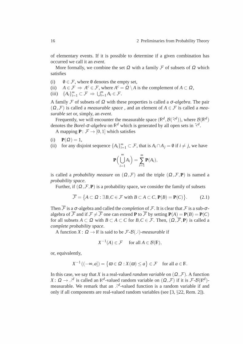
of elementary events. If it is possible to determine if a given combination hasoccurred we call it anevent.
More formally, we combine the setΩ with a familyF of subsets ofΩ whichsatisfies
(i) /0 ∈ F , where /0 denotes the empty set,(ii) A∈ F ⇒ Ac ∈ F , whereAc = Ω \A is the complement ofA⊂ Ω ,(iii) Ai∞
i=1 ⊂F ⇒ ⋃∞i=1Ai ∈ F .
A family F of subsets ofΩ with these properties is called aσ -algebra. The pair(Ω ,F) is called ameasurable space, and an element ofA∈ F is called amea-surable setor, simply, anevent.
Frequently, we will encounter the measurable space(Rd,B(Rd)), whereB(Rd)denotes theBorel-σ -algebraonRd which is generated by all open sets inRd.
A mappingP: F → [0,1] which satisfies
(i) P(Ω) = 1,(ii) for any disjoint sequenceAi∞
i=1 ⊂F , that isAi ∩A j = /0 if i 6= j, we have
P(
∞⋃
i=1
Ai
)
=∞
∑i=1
P(Ai),
is called aprobability measureon (Ω ,F) and the triple(Ω ,F ,P) is named aprobability space.
Further, if(Ω ,F ,P) is a probability space, we consider the family of subsets
F =
A⊂ Ω : ∃B,C∈ F with B⊂ A⊂C, P(B) = P(C)
. (2.1)
ThenF is aσ -algebra and called thecompletionof F . It is clear thatF is a sub-σ -algebra ofF and ifF 6=F one can extendP toF by settingP(A) = P(B) = P(C)for all subsetsA ⊂ Ω with B ⊂ A ⊂ C for B,C ∈ F . Then,(Ω ,F ,P) is called acomplete probability space.
A functionX : Ω → R is said to beF-B(R)-measurableif
X−1(A) ∈ F for all A∈ B(R),
or, equivalently,
X−1((−∞,a]) =
ω ∈ Ω : X(ω)≤ a
∈ F for all a∈ R.
In this case, we say thatX is a real-valuedrandom variableon(Ω ,F). A functionX : Ω → Rd is called anRd-valued random variable on(Ω ,F) if it is F-B(Rd)-measurable. We remark that anRd-valued function is a random variable if andonly if all components are real-valued random variables (see [3,§22, Rem. 2]).

2.2 Independence and Distributions of Random Variables 17
For example, the indicator function1A : Ω → R which is given by
1A(ω) =
1, for ω ∈ A,
0, for ω ∈ Ac,(2.2)
is a random variable if and only ifA∈ F .Next, as in [3,§9], we compactifyR to R by adding the points−∞ and∞. The
Borel-σ -algebraB(R) consists of all sets of the formB, B∪−∞, B∪+∞,B∪−∞,∞ with B∈ B(R). A F-B(R)-measurable functionX : Ω → R is calledanumerical function.
For a functionX : Ω → Rd we defineσ(X) to be the smallestσ -algebra onΩwhich contains all setsX−1(A) = ω ∈ Ω : X(ω) ∈ A with A∈ B(Rd). Conse-quently,X is σ(X)-B(Rd)-measurable and we sayσ(X) is theσ -algebra gener-ated by X.
Finally, let (X(t))t∈T with T ⊂ R be a family ofRd-valued random variables,that is for allt ∈ T the mapping
Ω ∋ ω 7→ X(t,ω) ∈ Rd
is a random variable. The family(X(t))t∈T is called astochastic processonT andfor a fixedω ∈ Ω the mapping
T ∋ t 7→ X(t,ω) ∈ Rd
is called asample pathof the process. As usual in stochastic analysis, we oftensuppressω as an argument of a random variable.
We will come back to the theory of stochastic processes in Chapter 6.
2.2 Independence and Distributions of Random Variables
This section is based on [22, Ch. 1.2] and [4,§3].We fix a probability space(Ω ,F ,P) and a measurable space(Ω ′,F ′). Consider
a measurable functionX : Ω → Ω ′. Then, for anyA′ ∈ F ′ the number
PX(A′) := P(X−1(A′)) = P(ω ∈ Ω : X(ω) ∈ A′) (2.3)
is well-defined. In fact, the mappingF ′ ∋ A′ 7→ P(X−1(A′)) is a probability mea-sure on(Ω ′,F ′), the image measure induced by X(see [3,§7]). In probabilitytheory the image measurePX is also denoted byX P and called thedistributionof the random variable X.
18 2 Preliminaries from Probability Theory
If (Ω ′,F ′) = (R,B(R)) the distribution ofX is completely characterized by thecumulative distribution function F: R→ [0,1] (c.d.f. for short), which is given by
F(x) = P(X ≤ x) = PX((−∞,x]) for all x∈ R. (2.4)
The cumulative distribution function is increasing and right-continuous and sat-isfies limx→∞ F(x) = 1, limx→−∞ F(x) = 0. Conversely, any function with theseproperties generates a probability measure on(R,B(R)) (see [31] and note thatthe reference [3, Theorem 6.6] uses left-continuous distribution-functions with(−∞,x) instead of(−∞,x] in (2.4)).
Now, we come to the very important concept of independent random variables.For a formal definition we refer to [4,§7]. Here we will work with the followingcharacterization [4, Th. 7.2].
Theorem 2.1.Consider a finite family of measurable spaces(Ωi ,Fi), i = 1, . . . ,n.A finite family(Xi)
ni=1 of random variables Xi : Ω → Ωi is independent if and only
if
P(
X1 ∈ A1, . . . ,Xn ∈ An)
=n
∏i=1
P(
Xi ∈ Ai)
(2.5)
for all Ai ∈ Fi, i = 1, . . . ,n.
As it is proved in [4,§7] it is enough to show (2.5) for all setsAi from a ∩-stable generator of theσ -algebraFi. For example, let(Ωi ,Fi) = (R,B(R)) forall i = 1, . . . ,n. Then a finite family of real-valued random variables(Xi)
ni=1 is
independent if and only if (2.5) holds for all half-open intervalsAi = [ai ,bi).Further, in the situation of Theorem 2.1 consider the mapping Y : Ω → Ω1×
. . .×Ωn which is given by
Y(ω) = (X1(ω), . . . ,Xn(ω)).
ThenY is aF-⊗n
i=1Fi-measurable random variable, where⊗n
i=1Fi denotes theproduct-σ -algebra. The distributionPY of Y is called thejoint distribution of(Xi)
ni=1. The following characterization is a consequence of Theorem 2.1 and
proved in [4, Th. 7.5].
Theorem 2.2.A finite family of random variables(Xi)ni=1 is independent if and
only if
PY = PX1 ⊗ . . .⊗PXn.

2.3 Integrability and Moments of Random Variables 19
Now we turn to the independence of infinitely many random variables(Xi)∞i=1
which map into measurable spaces(Ωi ,Fi). As in [4, §7] we say that the family(Xi)
∞i=1 is independent if and only if every choice of finitely many random vari-
ables(Xi)i∈I with I ⊂ N is independent. By [4, Th. 9.4] the statement of Theorem2.2 stays valid for the casen= ∞.
We also recall the following useful result.
Theorem 2.3.Let (Xi)i∈I be a finite or infinite family of random variables withvalues in measurable spaces(Ωi ,Fi). Consider measurable mappings Yi : Ωi →Ω ′
i . Then the family of random variables(Zi)i∈I given by Zi :=Yi Xi is indepen-dent.
For the proof we refer to [4, Th. 7.4].We call a family of random variables(Xi)i∈I with I ⊂ N independent and iden-
tically distributed, for shorti.i.d., if the family is independent andPXi = PXj forall i, j ∈ I .
In the following we often assume that an i.i.d. sequence(Xi)∞i=1 of random
variables is given. In probability theory this is a common assumption and it is easyto construct a probability space(Ω ,F ,P) and a sequence(Xi)
∞i=1 of measurable
mappings such that the(Xi)∞i=1 are i.i.d. with an arbitrary target distributionPX.
For this realization problem we refer to [4,§9].
2.3 Integrability and Moments of Random Variables
As above, we fix a probability space(Ω ,F ,P). Consider a real-valued randomvariableX : Ω → R. We say thatX is integrablewith respect to the probabilitymeasureP if the integral
E[X] := EP[X] :=∫
ΩX(ω)dP(ω)
exists. In this case we callE[X] theexpectationor mean valueof X.Following [3, Th. 12.2] we have thatX is integrable if and only ifE[|X|]<∞. By
L1(Ω) := L1(Ω ,F ,P;R) we denote the set of all integrable real-valued randomvariables on(Ω ,F ,P).
Since forα ∈ R andX,Y ∈ L1(Ω) it also holds that(αX),(X +Y) ∈ L1(Ω)with
E[
αX]
= αE[
X]
, andE[
(X+Y)]
= E[
X]
+E[
Y]
,
we obtain thatL1(Ω) is a vector space.Further, we have the inequalities (see [3, Th. 12.4])
20 2 Preliminaries from Probability Theory
∣
∣E[X]∣
∣≤ E[
|X|]
and for allX,Y ∈ L1(Ω) with X ≤Y it holds that
E[X]≤ E[Y].
Therefore, the mappingX 7→ E[X] is an isotone linear form onL1(Ω).Given p≥ 1 we say thatX is p-integrableif |X|p is integrable, that is
E[
|X|p]
=∫
Ω|X(ω)|pdP(ω)< ∞.
The valueE[
|X|p]
is called thep-th momentof X. Note that the setLp(Ω) of allrandom variablesX with existingp-th moment forms a subspace ofL1(Ω). In thecasep= 2 we also say thatX is square-integrablewith respect toP.
As in [3, §14] we assign the seminorms
Np(X) :=(
∫
Ω|X(ω)|pdP(ω)
) 1p
to the spacesLp(Ω) for p≥ 1. In particular, the seminorm satisfies
Np(αX) = |α|Np(X) for all α ∈ R,X ∈ Lp(Ω),
andMinkowski’s inequality
Np(X+Y)≤ Np(X)+Np(Y) for all X,Y ∈ Lp(Ω).
A further important inequality isHolder’s inequality
N1(XY)≤ Np(X)Nq(Y) for all X ∈ Lp(Ω),Y ∈ Lq(Ω),
with p,q > 1, 1p +
1q = 1. A generalized version of Holder’s inequality is found
in [1, Lem. 1.16]: Forn ∈ N andXi ∈ Lpi(Ω), i = 1, . . . ,n, with pi ∈ [1,∞) andr ∈ [1,∞) which satisfy
1r=
n
∑i=1
1pi
we have
Nr
( n
∏i=1
Xi
)
≤n
∏i=1
Npi(Xi).

2.3 Integrability and Moments of Random Variables 21
The seminormNp turns into a norm if we identify random variables whichcoincide almost surely. To be more precise, we say that two random variablesXandY are equalP-almost surelyor with probability1, if there exists a measurablesetN ∈ F with P(N) = 0 such that
X(ω) =Y(ω) for all ω ∈ Ω \N.
For short we writeX =Y a.s.Since it holds that
Np(X) = 0 ⇔ |X|p = 0 a.s. ⇔ |X|= 0 a.s. ⇔ X = 0 a.s.,
the set
N = N−1p (0)
is a linear subspace ofLp(Ω). As noted in [3,§15] the subspaceN is independentof p and the quotient vector space
Lp(Ω) := Lp(Ω)/N
is well-defined. By defining
‖X‖Lp(Ω) := Np(X)
for an equivalence classX ∈ Lp(Ω) and an arbitrary elementX of X we obtain anorm onLp(Ω). In fact, (Lp(Ω),‖ · ‖Lp(Ω)) is a Banach space [3, Th. 15.7]. Forprobability spaces it holds thatLp(Ω)⊂ Lq(Ω)⊂ L1(Ω) wheneverp≥ q≥ 1.
Note that in our notation we usually make no difference between random vari-ablesX ∈ Lp(Ω) and their equivalence classesX ∈ Lp(Ω).
Of special interest is the casep= 2. By setting
(X,Y) = E(XY) =∫
ΩX(ω)Y(ω)dP(ω) for X,Y ∈ L2(Ω)
we obtain an inner product and the spaceL2(Ω) becomes a Hilbert space.Another useful inequality isJensen’s inequality. Let J ⊂ R denote an interval
which contains the range of a random variableX ∈ L1(Ω) and consider a convexfunctionϕ : J → R such thatϕ(X) ∈ L1(Ω). Then Jensen’s inequality
ϕ(E[X])≤ E[ϕ(X)]
holds. For a proof we refer to [5, p. 276] (see also Problem 2.22).

22 2 Preliminaries from Probability Theory
Next, we introduce thevarianceof a random variable. The variance of a real-valued random variableX is defined by
var(X) = E[
(X−E[X])2].
If X ∈ L2(Ω) then var(X)< ∞. The square root of the variance is called thestan-dard deviation of Xand often used in statistics to measure the spread ofX aroundits mean. A simple calculation shows
var(X) = E[
X2]−(
E[X])2. (2.6)
If Y is another real-valued random variable, we call
cov(X,Y) = E[
(X−E[X])(Y−E[Y])]
thecovarianceof X andY. If cov(X,Y) = 0 we say thatX andY areuncorrelated.In particular, ifX andY are independent then it follows that cov(X,Y) = 0. More-over, if (Xi)
ni=1 are pairwise uncorrelated random variables then it holds that (see
[4, Th. 8.3])
var(X1+ . . .+Xn) = var(X1)+ . . .+var(Xn). (2.7)
This is due to the fact that
var(X+Y) = var(X)+2cov(X,Y)+var(Y). (2.8)
We conclude this section with a brief look atRd-valued random variablesX(ω) = (X1(ω), . . . ,Xd(ω)). The mean ofX is given by
E[X] =(
E[X1], . . . ,E[Xd])
.
Following [4,§30] one defines the covariance ofX by
cov(X) = E[(X−E[X])(X−E[X])T ] ∈ Rd,d,
that is, cov(X) is a symmetric matrix with entries cov(Xi ,Xj). In fact, one canshow thatC is always negative semidefinite.
In the same way as above, vector valued random variables giverise to a scalarof Banach spacesLp(Ω ;Rd) with norm
‖X‖Lp(Ω ;Rd) :=(
∫
Ω‖X(ω)‖pdP(ω)
) 1p,
where‖‖ denotes the Euclidean norm inRd.

2.4 The Transformation Theorem for Integrals 23
2.4 The Transformation Theorem for Integrals
In this section we present some useful versions of the well-known substitutionrule which we first state for general measure spaces.
The first version is concerned with integration with respectto an image mea-sure. For this consider a measure space(Ω ,F ,µ), a measurable space(Ω ′,F ′)and anF-F ′ measurable mappingT : Ω → Ω ′. The mappingT induces an imagemeasure (see (2.3) or [3, Th. 7.5])
µ ′ := µT
on the measurable space(Ω ′,F ′).
Theorem 2.4.Let f′ be a numerical function onΩ ′. Then theµT-integrability off ′ is equivalent to theµ-integrability of f′ T. In case of integrability it holds that
∫
Ω ′f ′dµT =
∫
Ωf ′ T dµ.
For the proof we refer to [3,§19]. In the case of a probability space(Ω ,F ,P)and a random variableX which takes values in a measurable space(Ω ′,F ′) aprobabilistic version of Theorem 2.4 reads as follows:
Theorem 2.5.Let f′ be a numerical function onΩ ′. Then thePX-integrability off ′ is equivalent to theP-integrability of f′ X. In case of integrability it holds that
EPX
[
f ′]
= EP[
f ′ X]
.
In particular, for a real-valued random variable X thePX-integrability of the map-ping x 7→ x is equivalent to theP-integrability of X and we have
E[
X]
=∫
RxdPX(x).
The next theorem turns to Lebesgue integrals and is often called thegeneraltransformation theorem for integrals.
Theorem 2.6.Let G, G′ be open subsets ofRd, andΦ : G→ G′ a C1-diffeomor-phism of G onto G′. A numerical function f′ on G′ is λ d-integrable if and only ifthe function( f ′ Φ)|detDΦ | is λ d-integrable over G, and in this case
∫
G′f ′dλ d =
∫
G( f ′ Φ)|detDΦ |dλ d.
A proof can be found in [3,§19] or [2, Th. 8.4].
24 2 Preliminaries from Probability Theory
2.5 Some Standard Distributions
In this section we focus on random variables which take values in Rd. In partic-ular, we are interested in random variablesX whose distributionPX is absolutelycontinuouswith respect to the Lebesgue measureλ d onRd, that isPX(A) = 0 forall A∈ B(Rd) with λ d(A) = 0.
In this case, by the Radon-Nikodym theorem [3,§17], there exists a measurablefunction f : Rd → [0,∞) with
PX(A) =∫
Af (x)dλ d(x) for all A∈ B(Rd). (2.9)
The functionf is called theprobability density function(p.d.f. for short) ofX anduniquely determinedλ d-almost surely. In addition to (2.9), aB(Rd)-measurablefunctionh : Rd → R is integrable with respect toPX if and only if h f is Lebesgueintegrable, and in this case we have
∫
Rdh(x)dPX(x) =
∫
Rdh(x) f (x)dx. (2.10)
Ford = 1, the cumulative distribution functionF : R→ [0,1] of X satisfies
F(x) = P(
X ∈ (−∞,x])
=∫ x
−∞f (y)dy.
The following examples are well-known standard distributions.
Example 2.7 (Uniform distribution).Fora,b∈ R with a< b we say that a randomvariableX is uniformly distributedon the interval[a,b) if it has the probabilitydensity function
f (x) =
1b−a, x∈ [a,b),
0, otherwise.
For short, we writeX ∼U(a,b).
Example 2.8 (Normal distribution).A normal or Gaussian random variable Xwith meanµ ∈ R and varianceσ2, σ > 0, has the probability density function
f (x; µ,σ2) =1
σ√
2πexp(
− (x−µ)2
2σ2
)
, for all x∈ R.
For short, we writeX ∼ N(µ,σ2). In fact, we have thatE(X) = µ and var(X) =σ2.
We say thatX is standard normally distributedif µ = 0 andσ = 1. It holds thatσX+µ ∼ N(µ,σ) if X ∼ N(0,1).

2.6 Conditional Expectations 25
Example 2.9 (Normal distribution inRd). As in [4, §30] we say that anRd-valuedrandom variableX is normally distributed, if for all linear formsℓ : Rd → R, ℓ 6= 0there exist valuesµℓ ∈ R andσℓ > 0 such that
ℓ(X)∼ N(µℓ,σℓ).
Set
µ := E[X] ∈ Rd and C := cov(X) ∈ Rd,d. (2.11)
If X is normally distributed, then its distribution is uniquelydetermined byµ andC. For short, we writeX ∼ N(µ,C).
If C is invertible, then the density ofX is given by
f (x; µ,C) = (2π)−d2 (det(C))−
12 exp
(
− 12(x−µ)tC−1(x−µ)
)
(2.12)
for all x∈ Rd. While the proof thatX has this distribution is somewhat advancedand uses Fourier transform [4, Satz 30.2] it is easy to show that a random variablewith p.d.f. (2.12) satisfies (2.11), see Exercise 2.19.
Example 2.10 (Chi-square distribution).If Z1, . . . ,Zr , r ≥ 1, are independent andN(0,1)-distributed random variables, then the sum of their squares arechi-square(χ2) distributed withr degrees of freedom, that is
X =r
∑i=1
Z2i ∼ χ2
r .
For a proof we refer to Problem 2.21. The probability densityfunction of the chi-square distribution is given by
f (x; r) =
2−r2Γ ( r
2)−1x
r2−1e−
12x, if x≥ 0,
0, if x< 0,
whereΓ denotes theGamma function. The chi-square distribution is a special caseof thegamma distributionand often arises in statistical tests.
2.6 Conditional Expectations
In this section we briefly review the concept ofconditional expectations. For thereader who is unfamiliar with this topic the probabilistic name is somewhat con-fusing since unlike the expectation of a random variable, the conditional expecta-tion is in general not a real number but a random variable. Here we present twodifferent approaches to define the conditional expectation.
26 2 Preliminaries from Probability Theory
As usual a probability space(Ω ,F ,P) is given. The first thing one may asso-ciate with the word “conditional” is perhaps theconditional probability of A∈ Funder condition B∈ F with P(B)> 0 which is given by
P(
A|B)
=P(A∩B)
P(B).
This is the probability of the eventA if we already know that the eventBwill occur.The concept of conditional expectations aims to generalizeconditional probabili-ties to a family of conditions.
First, we follow [4, §15] and present the definition which makes use of theRadon-Nikodym theorem [3,§17]. Let X ∈ L1(Ω) be given and consider a sub-σ -algebraG ⊂ F . In generalG contains significantly less events thanF and wecannot expectX to beG-measurable. Therefore the question arises: How doesXbehave if we assume that only events fromG occur? To answer this question welook for a random variableY which is measurable with respect toG and satisfies
E[1AX] =∫
AX dP=
∫
AYdP= E[1AY] for all A∈ G. (2.13)
We findY by noting that the mapG ∋ A 7→ E[1AX] defines a signed measure onthe measure space(Ω ,G,P|G) that is absolutely continuous with respect toP|G .ThenY is its Radon-Nikodym density function which is uniqueP-almost surely.We have
∫
AYdP|G =
∫
AX dP for all A∈ G.
But for A∈ G we have∫
AYdP|G =∫
AYdP so that (2.13) follows. In the followingwe will always use the symbolP when we integrateG-measurable functions withrespect to the restrictionP|G .
We say thatY is theconditional expectation of X under the conditionG and weuse the notation
E[X|G] :=Y.
If X is G-measurable thenX andY coincide.Before we discuss the properties ofE[X|G] we present an alternative way to de-
fine the conditional expectation. For this note thatL2(Ω ,G,P;R) is a closed sub-space ofL2(Ω ,F ,P;R). Therefore, sinceL2(Ω ,F ,P;R) is a Hilbert space thereexists the orthogonal projectorQG ontoL2(Ω ,G,P;R) which satisfies
E[XZ] = (X,Z)L2(Ω) = (QG(X),Z)L2(Ω) = E[QG(X)Z] (2.14)

2.7 Limit Theorems 27
for all X ∈ L2(Ω ,F ,P;R), Z ∈ L2(Ω ,G,P;R). In particular, (2.14) holds for allZ = 1A with A ∈ G and, thus,QG(X) satisfies (2.13). By the uniqueness of theconditional expectation it follows thatE[X|G] = QG(X).
Without going into details, by using the density ofL2(Ω)-functions inL1(Ω)it is possible to extend the projectorQG to functions inL1(Ω) such thatQG(X) =E[X|G] for all X ∈ L1(Ω).
We conclude this section by stating useful properties of theconditional expec-tation. This list can be found in [22, Ch. 1.3]. For proofs we refer to [4,§15] and[5, Sec. 34].
G = /0,Ω ⇒ E[X|G] = E[X]1Ω ,
X ≥ 0 ⇒ E[X|G]≥ 0,
X is G-measurable ⇒ E[X|G] = X,
X ≡ c ⇒ E[X|G] = c,
a,b∈ R ⇒ E[aX+bY|G] = aE[X|G]+bE[Y|G],X is G-measurable ⇒ E[XY|G] = XE[Y|G],
G1 ⊂ G2 ⊂F ⇒ E[E[X|G2]|G1] = E[X|G1].
Also useful is aconditional version of Jensen’s inequality.
Lemma 2.11.Let J⊂ R denote an interval containing the range of X∈ L1(Ω). Ifϕ(X) ∈ L1(Ω) for a convex functionϕ : J → R then it holds that
ϕ(
E[X|G])
≤ E[
ϕ(X)|G]
.
For the proof we refer to [5, p. 449] (see also Problem 2.22).Problem 2.23 asks the reader to investigate a link between the conditional prob-
ability and the conditional expectation.
2.7 Limit Theorems
Several fundamental theorems in probability theory describe the limit behavior ofaverages of independent and identically distributed random variables. We beginwith the strong Law of Large Numbers (LLN). A proof of the following theoremis found in [4, Satz 12.1].
Theorem 2.12.Let (Xi)i∈N be a sequence of pairwise independent real valuedrandom variables identically distributed withE(Xi) = η , i ∈N. Then the followingconvergence holds almost surely,
28 2 Preliminaries from Probability Theory
1n
n
∑i=1
Xi → η as n→ ∞, (2.15)
that is there exists a set A∈ F with P(A) = 0 such that
limn→∞
1n
n
∑i=1
Xi(ω) = η for ω /∈ A. (2.16)
Sometimes almost sure convergence is also denoted as convergence almost every-where (a.e. for short). There are other notions than almost sure convergence thatwill play a role in the following. We list them in the following definition.
Definition 2.13.Let Yn,n ∈ N andY be random variables on a probability space(Ω ,F ,P). Then one says thatYn converges toY
- in Lp or in p-th meanwith p≥ 1, if
E(|Yn−Y|p) = ‖Yn−Y‖pLp → 0 as n→ ∞,
- in probability, if for all ε > 0,
P(|Yn−Y| ≥ ε)→ 0, as n→ ∞,
- weakly(or in distribution), if for all continuous bounded functionsϕ ∈ Cb(R)
∫
Ωϕ dPYn →
∫
Ωϕ dPY as n→ ∞.
The notion of convergence in distribution comes from the fact (see [3, Satz 30.13,§30 Aufgabe 7]) that weak convergence is equivalent to the statement that thec.d.f.’sFn,F of Yn,Y satisfy for allx∈ R whereF is continuous,
Fn(x)→ F(x) as n→ ∞.
The relation between these various notions of convergence is illustrated by thefollowing implications (cf. [4,§5])
Lp-convergence=⇒ L1-convergence =⇒almost sure convergence=⇒
convergence in probability,
convergence in probability=⇒ weak convergence.(2.17)
The Central Limit Theorem (CLT) gives more information about the error ofconvergence in (2.15). The simplest version assumes an i.i.d. sequence of randomvariables with identical variance (see [5, Th. 27.1]).
2.7 Limit Theorems 29
Theorem 2.14. (De Moivre-Laplace, CLT)Let (Xi)i∈N be an i.i.d. sequence ofsquare integrable random variables with expectationE(Xi) = η and variancevar(Xi) = σ2 for i ∈ N. Then
Sn =1
σ√
n
n
∑i=1
(Xi −η)−→ N(0,1) as n→ ∞ in distribution. (2.18)
SinceN(0,1) has continuous c.d.f.FN(0,1) the convergence of the c.d.f.’sFSn isuniform (cf. [3, Th.30.13]), i.e.
||FSn −FN(0,1)||∞ = supx∈R
|FSn(x)−FN(0,1)(x)| → 0 as n→ ∞.
Moreover, by the theorem of Berry and Esseen (see [4, eq. (28.23)]) one has anestimate of the form
‖FSn −FN(0,1)‖∞ ≤ 6σ3
√n
E(|X1−η |3), (2.19)
provided the random variables have finite third moments. Theorder of conver-genceO(n−
12) in this estimate cannot be improved in general.
Theorem 2.14 holds under much weaker assumptions on the random variablesXi than stated above, see the Lindeberg conditions in [4,§28]. It is only assumedthat theXi are independent with expectationηi =E(Xi) and varianceσ2
i = var(Xi).The sumSn in (2.18) is then replaced by
Sn =1sn
n
∑i=1
(Xi −ηi), s2n = var(
n
∑i=1
Xi) =n
∑i=1
σ2i ,
and the Berry and Esseen estimate (2.19) generalizes to
‖FSn −FN(0,1)‖∞ ≤ 6s3n
n
∑i=1
E(|Xi −ηi |3). (2.20)
Finally, we also note the following multidimensional version of the central limittheorem (see [5, Th. 29.5]).
Theorem 2.15.Let Xi = (Xi,1, . . . ,Xi,d) be an i.i.d. sequence of square integrablerandom vectors with values inRd. Setµ := E[Xi] ∈ Rd and C:= cov(Xi) ∈ Rd,d
for i ∈ N. Then
Sn =1√n
n
∑i=1
(Xi −µ)−→ N(0,C) as n→ ∞ in distribution.

30 2 Preliminaries from Probability Theory
Exercises
Problem 2.16.Prove the following statement: IfX,Y,Z are independent randomvariables, then so are
(i) (X+Y) andZ,(ii) XY andZ.
Problem 2.17.Given a random variableX : Ω → R with probability density func-tion f : R→ [0,∞), determine the probability density function of
(i) X+a, for a∈ R,(ii) bX, for b 6= 0,(iii) exp(X),(iv) X2.
Problem 2.18.(i) Show that var(X) = E[X2]− (E[X])2.(ii) Calculate the first and second moments and the variance ofa random vari-
ableX : Ω → N0 with a Poisson distribution, i.e. for someλ > 0,
pn = P(X = n) =λ n
n!exp(−λ ) for n= 0,1, . . . .
Problem 2.19.Let C ∈ Rd,d be a symmetric, positive definite matrix and letX beanRd-valued random variable with density function
f (x; µ,C) = (2π)−d2(
det(C))− 1
2 exp(
− 12(x−µ)TC−1(x−µ)
)
whereµ ∈ Rd. Show thatE[X] = µ and cov(X) =C.Hint: Substitutey=C− 1
2(x−µ).
Problem 2.20.Let (Xi)ni=1 be a finite family of i.i.d.N(0,1) random variables.
For an orthogonal matrixV ∈ Rn,n consider the random vectorY := VX, whereX := (X1, . . . ,Xn)
T . Show that the componentsYi, i = 1, . . . ,n, of Y are also afinite family of i.i.d. N(0,1) random variables.
Hint: Use without a proof that a finite family ofN(0,1)-distributed randomvariables is independent if and only if they are pairwise uncorrelated.
Problem 2.21.TheGamma distributionΓ (a,b) with parametersa,b> 0 has thedensity function
f (x;a,b) =
ba 1Γ (a)x
a−1e−bx, x> 0,
0, x≤ 0,
with Γ (a) =∫ ∞
0 ta−1e−t dt. Prove the following statements:

2.7 Limit Theorems 31
(i) If (Xi)i=1,...,n are independent withXi ∼ Γ (ai ,b), thenn
∑i=1
Xi ∼ Γ(
n
∑i=1
ai ,b).
Hint: Use that the density of a sum of two independent random variable isthe convolution of their respective densities.
(ii) Let Z be a real-valued random variable withZ ∼ N(0,1). Then Z2 ∼Γ(1
2,12
)
.(iii) Let (Zi)
ni=1 be independent andN(0,1)-distributed random variables. Then
their sum is chi-square distributed, that isn
∑i=1
Z2i ∼ χ2
n.
Problem 2.22.Let ϕ : Rn → R be a two-times differentiable function such that theHessian matrix Hess(ϕ)(x) is nonnegative definite for allx∈ Rn.
(i) Show that
ϕ(x)≥ ϕ(y)+Dϕ(x)(y−x) andϕ(x+y
2
)
≤ 12
(
ϕ(x)+ϕ(y))
for all x,y∈ Rn.(ii) ProveJensen’s inequality, that is
ϕ(E[X])≤ E[ϕ(X)]
for an arbitrary random variableX : Ω → Rn.(iii) For a given sub-σ -algebraG ⊂ F prove the conditional version of Jensen’s
inequality
ϕ(E[X|G])≤ E[ϕ(X)|G]for an arbitrary random variableX : Ω → Rn.
Problem 2.23.Let (B j)nj=1 be a finite partition ofΩ , that is
n⋃
j=1
B j = Ω , B j ∈ F , P(B j)> 0, B j ∩Bk = /0 for j 6= k.
SetG = σ((B j)nj=1). ForX ∈ L1(Ω) show that
E[X|G] =n
∑j=1
E[1B j X]
P(B j)1B j .
By using this, derive forX = 1A with A∈ F that
E[X|G](ω) = P(A|B j) for all ω ∈ B j .

Chapter 3Generating Random Numbers
In this section we describe different approaches to generate random numbers. Inparticular, we discuss some algorithms which producepseudo-random numbers.The goodness of these algorithms is analysed through a set ofstatisticaltests. Atthe end of this section we have a look at the Mersenne Twister,which is a widelyused pseudo-random number generator.
3.1 Motivation
As it was pointed out in the introduction there exists a growing interest in mod-elling real world phenomenas which appear to be random. But before we can use acomputer to get any insights from one of these models we are facing the very ele-mentary problem that we work with a completely deterministic machine to modelrandom behaviour. So we are in need of some source of randomness.
The first approaches to overcome this problem were built-in physical devicesin computers which generated random numbers by atomic decayor cosmic raycounters. Another possibility are large databases of random numbers which weregenerated by real random phenomena.
But in practice, these solutions have several shortcomings.For example, inmodern applications in finance it is important to recompute the value of stockoptions very fast after a significant change of one of the model parameters. Thus,it is too slow if our physical device gives only one random number every ten sec-onds or too expensive to buy a million of these devices to get sufficiently manyrandom numbers in the desired time horizon.
In that regard databases are better suited. But here we have the problem thatsuch a database may be too small or may take too much memory. A databasewith one billion random numbers takes already one gigabyte of memory if everyrandom number takes exactly one byte.
33
34 3 Generating Random Numbers
Another issue is that one can think of several physical or chemical processesthat could be used to generate random numbers. But they are only useful for sta-tistical purposes if one exactly knows their distribution,which may vary over time.
In this section we mainly consider another approach, the so called pseudo-random number generator (PRNG). These algorithms produce numbersU1,U2, . . .which are completely deterministic but mimic a certain random behaviour. In par-ticular, we will focus on generators whose outputs look likean independent andidentically distributed sequence ofU(0,1) random numbers. In today’s practice,PRNGs are most often used in statistical applications.
Which random source one should choose in practice depends on the importanceof the following criteria in the given application:
• Statistical properties,• Speed and efficiency,• Number of available random numbers,• Reproducibility.
In any case one should always be careful about using results which are de-rived with the help of random number generators. As N. Madraspoints out in[21, Ch. 2.3] it is only recommended to use random number generators whichhave been tested thoroughly. In critical applications, it is worth to run simulationstwice using different random number generators.
One may think of many more sources of randomness which are notmentionedhere. As a starting point to this very active research field werefer to the discussionin [10, Ch. 1]. Let us finally mention that, despite considerable progress in actualcomputations, the question of a proper notion of arandom sequenceremains oneof the fundamental problems in Mathematics, see the enlightening discussion in[16, Ch.3].
3.2 Pseudo-Random Number Generators
In this paragraph we loosely follow [9, Ch. 3.2.2] and [21, Ch. 2.2]. We give a def-inition of the class of generators which produce independent U(0,1)-distributedpseudo-random numbers and introduce some terminology. We conclude with threeexamples.
Since computers can only store values of finite accuracy it isnatural to considergenerators which produce random integers in a finite set0,1, . . . ,M −1. Thenthe outputX is transformed into a random numberU ∈ (0,1), for example, by anauxiliary function which dividesX by M.
More formally, we have the following

3.2 Pseudo-Random Number Generators 35
Definition 3.1.A pseudo-random number generator(PRNG) is given by a choiceof a positive integerM, a functionh: 0,1, . . . ,M−1k → 0,1, . . . ,M−1 anda deterministic recurrence relation
Xi = h(Xi−k,Xi−k+1, . . . ,Xi−1) i ≥ k
for some fixed integerk ≥ 1. The required initial vector(X0, . . . ,Xk−1) is calledtheseed.
So far, the definition does not require any statistical properties of the generatedsequence(Xi)i≥k. This connection is established by the next definition.
Definition 3.2.A U(0,1)-PRNGis a pseudo-random number generator togetherwith an auxiliary functiong : 0,1, . . . ,M − 1 → (0,1) such that the sequence(Ui)i≥k := (g(Xi))i≥k passes a set of tests which verify that the sequence(Ui)i≥k
has the same statistical properties as an independent and identically distributedsequence ofU(0,1) random variables.
At this moment we stay somewhat vague about the set of statistical tests but wewill be more specific about this point in Section 3.4. Let us first prove the ratherobvious property that all PRNG cycle if we let them run long enough. The nextlemma is taken from [9, Lemma 3.1].
Lemma 3.3.For every PRNG and every seed(X0, . . . ,Xk−1) there exist positiveintegersα,β ∈ N such that Xi+β = Xi for all i ≥ α.
Proof. Since there exist at mostM different outcomes there are at mostMk dif-ferentk-tuples. Thus, afterMk iterations somek-tuple(Xi , . . . ,Xi+k−1) must haveoccurred before. Letα ∈ N be such that the tuple(Xα , . . . ,Xα+k−1) is the first toreappear and letβ ≥ 1 be the smallest number such that(Xα+β , . . . ,Xα+β+k−1) =(Xα , . . . ,Xα+k−1). Since the iterates are determined by the deterministic functionh we findXi+β = Xi for all i ≥ α by induction. ⊓⊔
Note that we take minimal numbersα,β in the proof and that these satisfyα ∈ 0, . . . ,Mk−1, β ∈ 1, . . . ,Mk. We call the numberβ = β (X0, . . . ,Xk−1)theperiodof the PRNG given the seed(X0, . . . ,Xk−1). The number
p := inf(X0,...,Xk−1)∈S
β (X0, . . . ,Xk−1)
is called theperiodof the PRNG, which is now independent of the seed. Here theinfimum is taken over the setS ⊂ 0, . . . ,M−1k of all valid seeds. The numberMk is the trivial upper bound of the period.
The following three examples are taken from [21, Ch. 2].

36 3 Generating Random Numbers
Example 3.4 (RANDU).The RANDU generator is intended to be anU(0,1)-PRNG. This algorithm fits into our definition by settingk = 1, M = 231 and thefunctionh is given by the recursion
Xi+1 = 65539Xi mod 231.
Here, mod is understood in the usual way: Ifl is an integer andm is a positiveinteger, thenl modm is the uniquer ∈ 0, . . . ,m−1 such thatl = nm+ r forsome integern.
The auxiliary function is given byg(x) = xM . Note that for the seedX0 = 0 we
haveXi = 0 for all i. Therefore, we setS = 1, . . . ,M−1 as the set of all validseeds.
The RANDU generator was used in the IBM 360/370 library for manyyears,although it has rather poor statistical properties. Nevertheless, it is an importanthistorical example of a linear congruential generator (LCG). We will study LCGsin more detail in Section 3.3, where we also have a closer lookat RANDU.
Example 3.5 (The Middle-Square Method).This generator was proposed by Johnvon Neumann in 1949. Setk = 1, M = 105. The sequence(Xi)i≥0 is defined asfollows: Given is an integer 0≤ Xi < 105, that is, a number with up to four digits.Take the square ofXi and, if necessary, add leading zeros to obtain a number withexactly eight digits. ThenXi+1 is the integer consisting of the middle four digits.For example, letXi = 6553, thenX2
i = 42941809 andXi+1 = 9418.However, in practice the middle-square method is not a good pseudo-random
number generator since it possesses a relatively short period, some fixed points (0,100, 2500, 3792 and 7600) and short cycles (for example 540→ 2916→ 5030→3009) and, more seriously, many initial seeds converge to a fixed point or a shortcycle (for example, ifXi < 100 then the resulting sequence will converge to thefixed point zero).
Example 3.6 (Fibonacci generator).For this generator we setk= 2 andM a largepositive integer. The recursion is given by
Xi+1 = (Xi +Xi−1) modM.
As the other two examples, the Fibonacci generator does not give rise to a goodU(0,1)-PRNG. If we use the auxiliary functiong(x) = x
M and setUi = g(Xi),thenP(Ui <Ui+1 <Ui−1) = 0 compared to16 for i.i.d. U(0,1)-random variables.Compare further with Problem 3.13.

3.3 Linear Congruential Generators 37
3.3 Linear Congruential Generators
In the following we focus on a specific and historically important class of PRNGs.The presented material is taken from [9, Ch. 3.2], [21, Ch. 2.2].
Definition 3.7.A linear congruential generator(LCG) is a pseudo-random num-ber generator withk = 1 and the functionh : 0, . . . ,M−1 → 0, . . . ,M−1 isgiven by
h(x) = (ax+c) modM,
wherea,c∈ N with a> 0. In this case we call the generator the(a,c,M)-LCG.If c= 0 we say that the LCG ismultiplicative.
In this form LCGs were first proposed by D. H. Lehmer in 1951 [20]. SinceLCGs are relatively simple their statistical properties canbe analyzed mathemati-cally. Therefore, the decision if a given choice of parameters (a,c,M) produces agood PRNG does not only rely on passing a set of tests.
We already know an example: The RANDU generator in Example 3.4is themultiplicative(65539,0,231)-LCG.
Typically, we want to have LCGs with huge periods and, hence, we have toconsiderM very large. The following theorem characterizes LCGs with maximalperiods. For a proof we refer to [16, Ch. 3.2].
Theorem 3.8.The period of the(a,c,M)-LCG is M if and only if the followingconditions are satisfied
(i) c and M are relatively prime1,(ii) every prime factor of M divides a−1, and(iii) if 4 divides M, then4 divides a−1.
For example, ifM = 231 then the(a,c,M)-LCG has periodM if and only if cis odd anda= 4n+1 for somen≥ 1. In particular, there exists no multiplicativeLCG with periodM. In caseM is prime, Theorem 3.8 gives the conditionsc 6= 0modM,a= 1 modM, see Problem 3.14.
Although the last theorem is a very useful tool for finding parameter values(a,c,M) such that the resulting LCG posses a long period there exists anotherissue which causes LCGs to have poor statistical properties.As in [21, Ch. 2.2]we demonstrate this for the RANDU generator for whichd-tuples of consecutiveoutputs(Xi ,Xi+1, . . . ,Xi+d−1), i ≥ 0, always lie on hyperplanes inRd-space.
For the RANDU generator first note thata= 65539= 216+3. Now we have
1 Two nonnegative integersa andb are relatively prime if 1 is the greatest common divisor.

38 3 Generating Random Numbers
0.0 0.2 0.4 0.6 0.8 1.0U1
0.0
0.2
0.4
0.6
0.8
1.0U2
RANDU - 2D-tuples
Fig. 3.1 Plot of(Ui ,Ui+1) with i = 0, . . . ,4999 for the RANDU generator and seedX0 = 1.
Xi+2 = (216+3)Xi+1 mod 231
= (216+3)2Xi mod 231
= (0+6·216+9)Xi mod 231
= (6(216+3)−9)Xi mod 231
= (6Xi+1−9Xi) mod 231.
This shows thatXi+2−6Xi+1+9Xi is always divisible by 231 and henceXi+2−6Xi+1+ 9Xi = n231 for somen ∈ Z. Since 1≤ Xj < 231 for all j ≥ 0 it is alsoclear thatn∈ −5,−4, . . . ,9. Therefore, the triples(Xi ,Xi+1,Xi+2) lie on one ofat most 15 parallel hyperplanes inR3.
Thus, if one knows the values ofXi andXi+1, then the value ofXi+2 is containedin a set of up to 15 integer values. This strongly contradictsthe aim of generatingpseudo-random numbers which behave as if they were independent. In that casethe knowledge ofXi andXi+1 does not help to restrict the set of possible values ofXi+2.

3.3 Linear Congruential Generators 39
U10.20.4 0.6 0.8U
2 0.20.4
0.60.8
U3
0.2
0.4
0.6
0.8
RANDU - 3d-tuples
U10.20.4 0.6 0.8U
2 0.20.4
0.60.8
U3
0.2
0.4
0.6
0.8
RANDU - 3d-tuples
Fig. 3.2 Plot of (Ui ,Ui+1,Ui+2) with i = 0, . . . ,4999 for the RANDU generator and seedX0 = 1.
We illustrate this behaviour in Figures 3.1 and 3.2, where wedrew the tuples(Ui ,Ui+1) in Figure 3.1 and(Ui ,Ui+1,Ui+2) in Figure 3.2 fori = 0, . . . ,4999 andUi =
XiM . For the naked eye Figure 3.1 looks as expected, that is, the tuples seem
to be uniformly distributed over the unit-square. But in Figure 3.2 we see that thetriples lie in parallel hyperplanes.
In fact, the same phenomenon can also be observed in the unit square if oneuses sufficiently many tuples and zooms into a small subregion. We will furtherinvestigate this in Problem 3.16.
The following theorem, due to G. Marsaglia [23], shows that this behaviouris typical for all multiplicative LCGs. The proof of the first part is deferred toProblem 3.15.
Theorem 3.9.Let the sequence(Xi)i≥0 be generated by the(a,0,M)-LCG withseed X0 ∈ 1, . . . ,M−1. If k1,k2, . . . ,kd ∈ Z is any choice of integers such that
k1+k2a+k3a2+ · · ·+kdad−1 = 0 modM,
40 3 Generating Random Numbers
then all pointsπi = (XiM , . . . ,
Xi+d−1M ) ∈ [0,1)d, i ≥ 0, lie in one of the hyperplanes
defined by the equations
k1x1+k2x2+ · · ·+kdxd = 0,±1,±2, . . . .
There are at most
|k1|+ |k2|+ · · ·+ |kd|
of these hyperplanes which intersect the unit d-cube[0,1)d. Moreover, there isalways a choice of k1,k2, . . . ,kd such that all of the points(πi)i≥0 fall in fewer
than(d!M)1d hyperplanes.
For the RANDU example witha= 216+3 we have
a2−6a+9= 0 mod 231.
Therefore, Theorem 3.9 guarantees that triples lie in at most 16 hyperplanes whichis a good upper bound of the actual number 15 found above.
Because of this behaviour most LCGs are usually not recommended to be usedin Monte-Carlo simulations. However, since they are easily implemented and an-alyzed LCGs are still considered in practice.
For further reading we refer to the discussions in [10, Ch. 1.2] and [11, Ch. 2.1].In [9, Ch. 3.1] the authors give more details on how to choose the parameter valuea to get a period ofM−1 for multiplicative LCGs.
3.4 Empirical Tests
Definition 3.2 incorporated the condition that aU(0,1)-PRNG should pass a setof statistical tests to verify its statistical properties.In this paragraph we describehow these tests are designed. Here we follow [21, Ch. 2.2] and [10, Ch. 2].
Goodness-of-fit Test
In a goodness-of-fit test we want to test the hypotheses thatd-tuples formed fromthe output of aU(0,1)-PRNG is uniformly distributed in(0,1)d.
More formally, the test works in the following way:
(i) Choosen≥ 2 and a partition of[0,1]d into n disjoint subsetsS1, . . . ,Sn withcorresponding “volumes”p1, . . . , pn > 0.
(ii) For a given numberN > 0 of test vectors use the PRNG to generateN d-tuples(U1, . . . ,Ud), . . . ,(U(N−1)d+1, . . . ,UNd).

3.4 Empirical Tests 41
(iii) Then compute
X2n (N) :=
n
∑i=1
(σi −Npi)2
Npi,
whereσi denotes the observed number ofd-tuples which lie inSi.
The test generalizes the idea of making a histogram to visualize the density ofthe random numbers and is based on a theorem, which is due to K.Pearson. In oursituation the theorem reads as follows:
Theorem 3.10.If the d-tuples are generated from independent and U(0,1)-distributedrandom variables, then it holds that for all x∈ R
P(
X2n (N)≤ x
)
→ Fn−1(x) for N → ∞,
where Fn−1 denotes the cumulative distribution function of the chi-square distri-bution with n−1 degrees of freedom from Example 2.10.
For a proof we refer to [17, Th. 14.5].Hence, if thed-tuples generated with data from a PRNG behave as if they are
uniformly distributed in(0,1)d, then for largeN the computed valueX2n (N) should
also behave in the same way as a random variable that has an approximate chi-square distribution.
Therefore, large values ofX2n (N) indicate that the observed counts differ by
large amounts from the expected counts. A possible decisionrule is to reject thetested PRNG as aU(0,1)-PRNG if the value ofX2
n (N) is in the upper 5% of thetail of theχ2
n−1 distribution.The test should be repeated for several choices ofd, n, (Si)i=1,...,n, andN.
Quantile-Quantile Plot
A quantile-quantile plot is a graphical test which indicates if the random numbersgenerated by a PRNG follow the law of a given distribution. To some extent thiscan be seen as a variant of the goodness-of-fit test.
To be more precise, letP be a probability measure on(R,B(R)) and considerthe cumulative distribution-functionFP : R→ [0,1] given by
FP(x) = P(
(−∞,x])
(compare further with (2.4)).

42 3 Generating Random Numbers
Definition 3.11.For anyp∈ (0,1) the value
z(p) := inf
z∈ R | FP(z)≥ p
>−∞ (3.1)
exists and is called thep-th quantileof the measureP.
The functionz(·) is a partial inverse ofFP and also denoted byF−1P . By the right
continuity ofFP we always have
FP(z(p)) = FP(F−1P (p))≥ p, (3.2)
see Section 4.1 for an application. IfP is given by a probability density function(p.d.f.) f , that is
FP(x) = P(
(−∞,x])
=∫ x
−∞f (y)dy,
thenFP is indeed continuous and we haveFP(z(p)) = p. For further properties ofthe quantile function see Exercise 3.17.
The basic idea of a quantile-quantile plot is as follows: We are given a sequenceof pseudo-random numbers(Ui)i=1,...,N and we want to test the hypothesis that the(Ui)i=1,...,N follow the lawP. Thus, if this is true, for largeN, approximately onequarter of theUi should fall in each of the intervals(−∞,z(1/4)], (z(1/4),z(1/2],(z(1/2),z(3/4)],(z(3/4),∞). More generally, partition(0,1] into (pi−1, pi], i =1, . . .N wherepi =
iN and observe that a random variableU with continuous c.d.f.
FP satisfies
P(z(pi−1)<U ≤ z(pi)) = FP(z(pi))−FP(z(pi−1)) =1N.
Hence, if we generatekN valuesU j , j = 1. . .Nk we expect that, on average,kvalues lie in each interval(z(pi−1),z(pi)]. In the extreme casek = 1 every in-terval (z(pi−1),z(pi)] is hit, on average, by one random numberU j , j = 1, . . .N.Therefore, if(U j) j=1,...,N denotes the given sequence of pseudo-random numbers(U j) j=1,...,N in increasing order then we should see something close to a straightline if we draw the tuples(Ui ,z(pi)) for i = 1, . . . ,N.
We demonstrate this in Figure 3.3. There we generate a sequence of pseudo-random numbers with the RANDU generator (see Example 3.4) andanother withthe Fibonacci generator (see Example 3.6) .
Since both generators are supposed to beU(0,1) generators we have to deter-mine the distribution-functionFU(0,1). We get
FU(0,1)(x) =∫ x
−∞1(0,1)(y)dy= x for x∈ (0,1).

3.4 Empirical Tests 43
0.0 0.2 0.4 0.6 0.8 1.0sorted samples
0.0
0.2
0.4
0.6
0.8
1.0
U(0
,1) Q
uantile
RANDU
0.0 0.2 0.4 0.6 0.8 1.0sorted samples
0.0
0.2
0.4
0.6
0.8
1.0
U(0
,1) Q
uantile
Fibonacci Generator
Fig. 3.3 Quantile-Quantile Plots of sorted samples generated by RANDU (left hand pic-ture, seedX0 = 1000) and the Fibonacci generator (right hand picture, seedsX0 = 1000,X1 = 3456) plotted against the quantiles of theU(0,1) distribution. Number of samplesN = 500.
Hence, we obtainz(p) = p. Thus, in order to draw Figure 3.3 we simply sortedthe generated pseudo-random numbers and plotted the tuples(Ui , i/N) for i =1, . . . ,N.
As we can see, for both generators the plotted tuples lie close to the straightdashed linex 7→ x. Thus, both sequences behave in this test as if they are uniformlydistributed.
Runs Test
While a goodness-of-fit test and a quantile-quantile plot arestatic tests which donot take into account in which sequence the output is generated, a runs test is aso-called dynamic test. It is designed to test if a given output sequenceU1,U2, . . .behaves in the same way as a sequence which is generated by independent and

44 3 Generating Random Numbers
identically distributed random variables. But note that this test gives no informa-tion about the distribution of theUi.
In more detail, fixN ≥ 2 and letRN denote the statistic which records the num-ber of increasing or decreasing “runs” in the outputU1, . . . ,UN.
For example, forN = 10 consider the sequence
(0.55,0.57,0.54,0.08,0.29,0.24,0.20,0.80,0.67,0.91).
Then (0.55,0.57), (0.08,0.29), (0.20,0.80) and (0.67,0.91) are “up runs” and(0.57,0.54,0.08), (0.29,0.24,0.20) and(0.80,0.67) are “down runs”. Therefore,we haveR10 = 7. More formally, we have
RN = #i ∈ 2, . . . ,N−1 : (Ui+1−Ui)(Ui −Ui−1)< 0+1.
If the output is i.i.d. then one can show thatE(RN) = (2N−1)/3 and var(RN) =(16N− 29)/30 (compare Problem 3.18). Moreover, one can invoke the centrallimit theorem to show that(RN −E(RN))/
√
var(RN) converges in distribution toN(0,1) asN → ∞, The latter fact may then be used to formulate a decision rule.
Test Suits
There exist collections of standardized statistical testsfor U(0,1)-PRNG. We in-troduce some of the important suites.
DIEHARD is a battery of eighteen statistical tests which consists of sev-eral variants of the goodness-of-fit tests and runs tests. DIEHARD is due toG. Marsaglia and based on [24]. The source code of the tests isavailable at
http://www.stat.fsu.edu/pub/diehard/
A detailed presentation of the tests is found in [10, Ch. 2].A similar test suite is mainted by the National Institute of Standards and Tech-
nology (NIST) of the USA. The software and its documentationis found on thewebpage
http://csrc.nist.gov/rng/
A very extensive test suite is TestU01. It includes the testsfrom DIEHARDand NIST and many more. It is written in C and maintained by P. L’Ecuyer andR. Simard [19]. The source code and a detailed documentation is found on
www.iro.umontreal.ca/˜simardr/testu01/tu01.html

3.5 The Mersenne Twister 45
3.5 The Mersenne Twister
A nowadays widely used PRNG is the Mersenne Twister (MT) . For example,it is the built-in random number generator in the Python module Numpy and inMatlabR©, where it is used since version 7.4. The Mersenne Twister [27] was pro-posed by M. Matsumoto and T. Nishimura in 1998 and passed several statisticaltests including DIEHARD.
The MT-PRNG has a very huge period ofM = 219937−1, a Mersenne prime.Moreover, it is 623-equidistributed to 32-bit accuracy which is defined as follows.
Definition 3.12.A sequenceXi of w-bit integers of periodM is calledk-equi-distributed tob-bit accuracy if the following property holds. In each string oflengthkb
(Xi,b,Xi+1,b, . . . ,Xi+k−1,b), i = 0, . . . ,M−1,
whereXi,b is the string of the firstb bits of Xi, each of the possible 2kb combina-tions of bits occurs the same number of times, except for the all-zero combinationwhich occurs once less often. The largestk such thatk-equidistribution tob-bitaccuracy holds is denoted byk(b).
Note that this is a finite version of the equidistribution ofk-tuples chosen from ani.i.d. U(0,1)-sequence. For the parameters in (3.4) below it is shown in [27] thatk(b)≥ 623 holds forb= 1, . . . ,32, in particulark(1) = 19937,k(32) = 623.
For the rest of this section we sketch the idea behind the Mersenne Twister.For more details, in particular the choice of seeds, we referto the material on theauthors’ webpage2. The content of this section is based on [27].
The Mersenne Twister is a variant of the so called generalized feedback shiftregister (GFSR) generator. This generator makes use of very fast bit operationswhich correspond to the polynomial algebra over the two-element fieldF2.
Let Xi, i ≥ 0, denote aword vectorof dimensionw, where we usually havew = 32. More formally,Xi is a row vector with entries over the fieldF2. Thus,we can identifyXi with a machine word consisting ofw bits. The MT algorithmgenerates a sequence of word vectors(Xi)i≥0 which are then considered to beuniform pseudo-random integers between 0 andM = 2w−1.
We denote byX ⊕Y the addition of two row vectorsX,Y ∈ Fw2 . Moreover,
for a fixed integer 0≤ r ≤ w− 1 we define the upper and lower bits ofX =(xw−1, . . . ,x0) ∈ Fw
2 by
Xu = (xw−1, . . . ,xr), Xl = (xr−1, . . . ,x0).
The following linear recursion builds the core element of the algorithm
2 http://www.math.sci.hiroshima-u.ac.jp/ ∼m-mat/MT/emt.html

46 3 Generating Random Numbers
Xi+n = Xi+m⊕ (Xui |Xl
i+1)A, i = 0,1, . . . . (3.3)
In this recursion we have several integers, namelyn,m, r where 1≤ m< n,2≤ nand 0≤ r ≤ w−1 is hidden inside the definition ofXu
i . By A we denote aw×wmatrix with entries inF2 which will be specified below. Further,(·|·) denotes theconcatenation of aw− r bits vector and anr bits vector which together form awbits vector.
Therefore, in the right hand side of (3.3) the term(Xui |Xl
i+1)A means, that wethe take the upperw− r bits of Xi and the lowerr bits of Xi+1 and concatenatethese bits to a new word vector withw bits. Then this row vector is multipliedfrom the right by the matrixA, where this operation is done with respect to thefield F2. Finally, we obtainXi+n by addingXi+m to the matrix-vector product.
In order to make the matrix-vector multiplication very fast, the matrixA has thespecial form
A=
11
...1
aw−1 aw−2 · · · · · · a0
.
Then XA can be implemented by only using fast bit operations, since for X =(xw−1, . . . ,x0)
XA=
shiftright(X) if x0 = 0,shiftright(X)⊕a if x0 = 1,
where a = (aw−1, . . . ,a0) and shiftright(X) = (0,xw−1, . . . ,x1). The generatorMT19937 proposed in [27] uses the data
w= 32,n= 624,m= 397, r = 31. (3.4)
In the last step, we have to specify the auxiliary functiong which transforms theoutput sequence(Xi)i≥0 of random integers intoU(0,1) pseudo-random numbers.In order to improve the random behaviour of the least significant bits the authors ofMersenne Twister propose a so called tempering function. The tempering functionconsists of multiplyingXi with a second matrixT before interpreting thew-bits asan integer and dividing it byM = 2w−1. As above, also the matrixT is chosen insuch way that the matrix-vector product can be implemented as a sequence of bitoperations.
3.5 The Mersenne Twister 47
Exercises
Problem 3.13.Let (Xi)i≥1 be a sequence of natural numbers which is generatedby the Fibonacci-PRNG. Show thatP(Xi < Xi+1 < Xi−1) = 0, butP(Ui <Ui+1 <Ui−1) =
16 for an i.i.d.U(0,1)-sequence(Ui)i≥1.
Problem 3.14.Prove Theorem 3.8 for the special case whenM is a prime.Hint: Use Fermat’s theorem (aM = a modM for all primesM and integersa).
Problem 3.15.Prove the first part of Theorem 3.9. That is, givenk ∈ Zd with∑d
i=1kiai−1 = 0 mod M, then all pointsπi =1M (Xi , . . . ,Xi+d−1) ∈ [0,1)d, i ≥ 0
generated by the(a,0,M)-LCG with seedX0 ∈ 1, . . . ,M − 1 lie in one of thehyperplanes
Hn(k) = x∈ Rd : kTx= n, n∈ Z.There are at most∑d
i=1 |ki| such hyperplanes that intersect thed-cube[0,1)d.
Problem 3.16.Implement the RANDU-LCG in Matlab. For an arbitrary seedX0 6= 0 generate the firstN = 107 appropriately normalized pseudo random num-bers(Xi)
Ni=1 ⊂ [0,1], group them into pairs(Xi ,Xi+1), i = 1, . . . ,N− 1, and plot
only those pairs which lie in the subregion[0,0.001]× [0,1]. Interpret the resultin view of Theorem 3.9 and Figure 3.1.
Problem 3.17.Show that the quantile functionF−1P defined in (3.1) is monotone
increasing, left continuous and satisfies
F−1P (p) = supz∈ R : FP(z)< p.
Problem 3.18.For a runs test we are interested in the random variable
RN = #i ∈ 2, . . . ,N−1 : (Ui+1−Ui)(Ui −Ui−1)< 0+1, N ≥ 2.
(i) Show thatE[RN] = (2N−1)/3 if (Ui)Ni=1 is a family of i.i.d.U(0,1) random
variables.(ii) Show thatE[RN] = (2N− 1)/3 remains true if(Ui)
Ni=1 is a family of i.i.d.
random variables whose distribution is given by a continuous probability den-sity function f : R→ [0,∞).
Hint: For (ii) use integration by parts.

Chapter 4Generating Random Variables with Non-UniformDistribution
In this section we work under the general assumption that we have availablean endless stream of independent and identically distributed random numbers(Ui)i≥0, with known distribution. Our aim is to generate a second sequence ofi.i.d. random variables which follow a different distribution.
In practice, the(Ui)i≥0 will often be generated by aU(0,1)-PRNG from theprevious section. We will discuss general methods like the inverse transformationand the accept-reject-algorithm to produce an arbitrary target distribution. Then,we will focus on the Box-Muller method and Marsaglia’s Ziggurat method whichgenerate normally distributed random variables.
Literature: [30, Ch. 2], [10, Ch. 4 - 5], [11, Ch. 2.3] [21, Ch. 2.3]
4.1 Inversion Method
Suppose we are given a target cumulative distribution-function F : R→ [0,1] andaU(0,1) distributed random variableU . Then theinversion methoduses the quan-tile function (3.1) to generate a random variable with distribution F .
Proposition 4.1.Let F: R→ [0,1] be a distribution-function and let U be a ran-dom variable with U∼U(0,1). Then F−1(U)∼ F.
Proof. Recall from (3.1) that
F−1(U(ω)) = inf
ξ ∈ R : U(ω)≤ F(ξ )
.
Using (3.2) and the isotony ofF we find thatF−1(U(ω)) ≤ x is equivalent toU(ω) ≤ F(x) for every x ∈ R. Note that this also holds in caseU(ω) = 0 bysettingF−1(0) =−∞. Therefore,P(F−1(U)≤ x) = P(U ≤ F(x)) = F(x) and theassertion follows. ⊓⊔
49
50 4 Generating Random Variables with Non-Uniform Distribution
Of course, generating anF-distributed sequenceF−1(Ui) from the given sequenceUi needs an efficient algorithm for evaluatingF−1. In some cases this can be doneexplicitly.
Example 4.2.The exponential distribution Exp(λ ) with parameterλ > 0 has thedistribution-functionF(x) = 1− exp(−λx) for x ≥ 0 andF(x) = 0 for x < 0.By Proposition 4.1 the random variable− 1
λ log(1−U) then is exponentially dis-tributed.
One way of inverting a continuous distribution-functionF numerically is tocompute and store in advance the quantilesz1 < z2 < .. . < zk−1 such thatF(zi) =ik, i = 1, . . .k−1, wherek is sufficiently large. IfF is smooth then a Newton typemethod is suitable for doing this. Moreover, letz0 be the largest value such thatFcan be regarded as 0 to the left ofz0, and letzk be the smallest value such thatFcan be regarded as 1 to the right ofzk.
Then generate a pseudo random numberU and leti = ⌊kU⌋ so thatF(zi)≤U <F(zi+1). The value ofX is then determined approximately by one step of regulafalsi (linear inverse interpolation) from
X = zi +(zi+1−zi)U −F(zi)
F(zi+1)−F(zi)= zi +(zi+1−zi)(kU− i). (4.1)
4.2 Rejection Method
The rejection method (also calledacceptance/rejection method) is due to Johnvon Neumann. It generates a random variable with a given p.d.f. f by using twoindependentU(0,1) generators. The idea is to construct a box[a,b]× [0,c] thatcontains the graph (of the positive part) off , i.e. (x, f (x)) : x ∈ R, f (x) > 0.Then generate a random point(U,Y) in the box and acceptU if (U,Y) is belowthe graph (see Figure 4.1).
More precisely, choosea< b, 0< c such thatf (x) = 0 for x /∈ [a,b] and f (x)≤ cfor all x∈ [a,b]. Then perform the following
Simple rejection algorithm
1. GenerateU ∼U(a,b) from U = a+(b−a)U1 with U1 ∼U(0,1).2. GenerateY ∼U(0,c) from Y = cU2 with U2 ∼U(0,1).3. If Y ≤ f (U) thenaccept X=U , elsereject U and return to step 1.
This algorithm can be generalized for ad-dimensional p.d.f.f : Rd → R underthe assumption that we can generate another random variablewith p.d.f.g : Rd →R where for somec> 0,
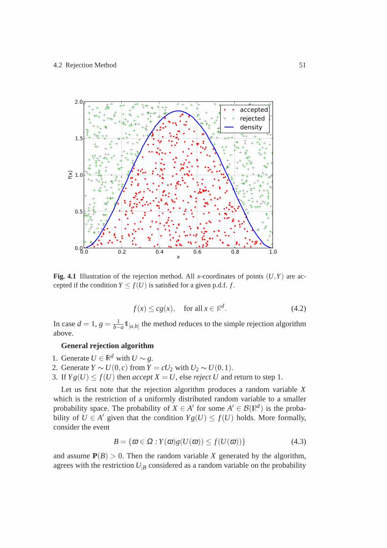
4.2 Rejection Method 51
0.0 0.2 0.4 0.6 0.8 1.0x
0.0
0.5
1.0
1.5
2.0
f(x)
acceptedrejecteddensity
Fig. 4.1 Illustration of the rejection method. Allx-coordinates of points(U,Y) are ac-cepted if the conditionY ≤ f (U) is satisfied for a given p.d.f.f .
f (x)≤ cg(x), for all x∈ Rd. (4.2)
In cased = 1, g= 1b−a1[a,b] the method reduces to the simple rejection algorithm
above.
General rejection algorithm
1. GenerateU ∈ Rd with U ∼ g.2. GenerateY ∼U(0,c) from Y = cU2 with U2 ∼U(0,1).3. If Yg(U)≤ f (U) thenaccept X=U , elsereject U and return to step 1.
Let us first note that the rejection algorithm produces a random variableXwhich is the restriction of a uniformly distributed random variable to a smallerprobability space. The probability ofX ∈ A′ for someA′ ∈ B(Rd) is the proba-bility of U ∈ A′ given that the conditionYg(U) ≤ f (U) holds. More formally,consider the event
B= ω ∈ Ω : Y(ω)g(U(ω))≤ f (U(ω)) (4.3)
and assumeP(B) > 0. Then the random variableX generated by the algorithm,agrees with the restrictionU|B considered as a random variable on the probability
52 4 Generating Random Variables with Non-Uniform Distribution
space(B,FB,PB) with FB = F ∩B and
PB(A∩B) = P(A|B) = P(A∩B)P(B)
, A∈ F . (4.4)
Theorem 4.3 (Fundamental Theorem of Simulation).The random variable Xgenerated by the general rejection algorithm has the probability density functionf .
Proof. Using (4.4) withA= U ∈ A′, A′ ∈ B(Rd), we obtain
PB(X ∈ A′) =P(U ∈ A′∩B)
P(B). (4.5)
SinceU andY are independent the joint distribution ofT = (U,Y) is the productof the single distributions (Theorem 2.2)
PT = PU ⊗PY = g(u)λ d(u)⊗ 1c1[0,c](y)λ 1(y).
ConsiderB′ = (u,y) ∈ Rd × [0,c] : yg(u) ≤ f (u). Since1B = 1B′ T the trans-formation theorem (Theorem 2.5) yields
P(B) =∫
1B′ T dP=∫
1B′ dPT
=∫
Rd
1c
∫
y∈[0,c]:yg(u)≤ f (u)dy g(u)du (4.6)
=∫
Rd
1c
f (u)du=1c.
The inner integral in (4.6) equalsf (u)g(u) ≤ c if g(u) > 0, and its value isc in case
g(u) = 0 (and hencef (u) = 0 by (4.2)). In the same way as above, replaceRd byA′ and find
P(U ∈ A′∩B) =∫
A′
1c
f (u)du.
Thus (4.5) yieldsPB(X ∈ A′) =∫
A′ f (u)du for all A′ ∈ B(Rd). ⊓⊔We discuss the numerical effort for the general rejection algorithm. By (4.6) the
probability that the algorithm accepts a valueU is 1c. Hencec is the expected num-
ber of proposals needed to generate one value ofX. We would like to minimizethis value while satisfying (4.2), i.e. the optimal value is
c= supg(x)>0
f (x)g(x)
. (4.7)

4.3 The Box-Muller Method 53
Example 4.4.Let us generate a random variableX ∼ N(0,1) by using a generatorfor a random variableU with p.d.f.g(x) = 1
2e−|x|,x∈ R. In this case (4.7) gives
c= supx∈R
2exp(−x2
2 )√2π exp(−|x|)
=
√
2π
supx≥0
exp(x− x2
2) =
√
2eπ
≈ 1.3155. (4.8)
The variableU can be generated by taking logarithms of aU(0,1)-distributedvariable with random signs (for a justification and an alternative via the inversionmethod see Problem 4.8)
1. Generate independentU1,U2 ∼U(0,1).2. SetU =− log(U2) if U1 ≤ 1
2 andU = logU2 otherwise.3. LetY = cg(U)U3 whereU3 ∼U(0,1).4. If
√2πY ≤ exp(−U2
2 ) then acceptX =U .
As for efficiency, we require an average of 3c≈ 3.9465 random numbers in orderto generate oneX-value. By (4.8) the test in step 4 can be simplified toU3 ≤exp(
−12(1−|U |)2
)
. For a more detailed efficiency analysis one should also countthe additional number of flops and function evaluations of log and exp.
4.3 The Box-Muller Method
This method uses polar coordinates in order to generate two i.i.d.N(0,1) variablesfrom two i.i.d.U(0,1) variables:
Box-Muller Method
1. Generate two independentU1 ∼U(0,1), U2 ∼U(0,1).2. SetX1 =
√−2logU1cos(2πU2), X2 =√−2logU1sin(2πU2).
Theorem 4.5 (Box-Muller Method). The Box-Muller Method generates two in-dependent N(0,1) distributed random variables X1,X2.
Proof. It is sufficient to show that for everyA∈ B(R2)
P(X1,X2)(A) = P((X1,X2) ∈ A) =∫
A
12π
exp(
− 12(x2
1+x22))
d(x1,x2). (4.9)
Following the proof in [12, Ch. 5.2] we consider the open setsG= R2\
(y,0) ∈R2 : y≥ 0 andG′ = (0,1)2 and define a functionh: G′ → G by
h(x) =
(√−2logx1cos(2πx2)√−2logx1sin(2πx2)
)
, x= (x1,x2) ∈ G′.
54 4 Generating Random Variables with Non-Uniform Distribution
Note thath is bijective with inverse
h−1(y) =
(
exp(
− 12|y|2
)
12π atan2(y)
)
, y= (y1,y2) ∈ G.
Here, atan2:G→ (0,2π) is given by
atan2(y) = atan2(y1,y2) =
arctan(
y2y1
)
, for y1, y2 > 0,12π, for y1 = 0, y2 > 0,
arctan(
y2y1
)
+π, for y1 < 0, y2 ∈ R,32π, for y1 = 0, y2 < 0,
arctan(
y2y1
)
+2π, for y1 > 0, y2 < 0.
By this definitionh−1 is continuously differentiable with
Dh−1(y) =
(
−y1x1 −y2x1
− 12π
y2y2
1+y22
12π
y1y2
1+y22
)
,
wherex1 = exp(−12|y|2). Therefore,h−1 is aC1-diffeomorphism ofG ontoG′.
Now, for all A∈ B(G) it holds that
P(X1,X2)(A) = P(
(X1,X2) ∈ A)
= P(
h(U1,U2) ∈ A)
= P(
(U1,U2) ∈ h−1(A))
.
Sinceh−1(A)⊂G′ is a measurable set, the functionf ′ : G′ → R, which is given bythe indicator functionf ′(u) = 1h−1(A)(u), is λ 2-integrable onG′. Hence, we areable to apply the general transformation theorem for integrals (see Theorem 2.6)and get
P(
(U1,U2) ∈ h−1(A))
=∫
G′1h−1(A)dλ 2 =
∫
G
(
1h−1(A) h−1)|detDh−1|dλ 2.
Next, we use
(
1h−1(A) h−1)(y) = 1h−1(A)(h−1(y)) = 1A(y),
and
∣
∣detDh−1(y)∣
∣=x1
2π=
12π
exp(
− 12|y|2)
.
Altogether, this proves the desired result for all measurable setsA∈ B(G), since

4.4 Marsaglia’s Ziggurat Method 55
P(X1,X2)(A) =∫
G1A(y)
12π
exp(
− 12|y|2)
dy
=1
2π
∫
Aexp(
− 12
(
y21+y2
2
)
)
d(y1,y2).
For generalA∈ B(R2) consider the decomposition in disjoint sets
A=(
A∩G)
∪(
A\G)
.
Then, we haveA∩G∈ B(G) and sinceλ 2(A\G) = 0 we get
P(X1,X2)(A∩G) =1
2π
∫
A∩Gexp(
− 12
(
y21+y2
2
)
)
d(y1,y2)
=1
2π
∫
Aexp(
− 12
(
y21+y2
2
)
)
d(y1,y2).
Thus, the proof is complete if it holds that
P(X1,X2)(A\G) = 0.
But this is true since
P(X1,X2)(A\G)≤ P(
sin(2πU2) = 0)
= P(
U2 ∈ 0,1)
= 0.
⊓⊔
4.4 Marsaglia’s Ziggurat Method
Because of the function evaluations involved, both the Box-Muller and the inver-sion method are considered to be quite expensive. A fast alternative method thatis nowadays used in MATLAB’srandn (algorithm mcg16807 since MATLAB5) is theZiggurat Methodproposed by Marsaglia and Tsang [25, 26]. The nameziggurat(in German:die Zikkurat) refers to the stepped pyramides with a templeon top that were built in ancient Mesopotamia (∼ 2100 B.C.) and that appearedas terraced pyramides about 3000 years later in Central America with the Aztecsand other peoples.
The ziggurat method is an improvement of the acceptance/rejection method inorder to increase the efficiency1
c and to reduce the number of function evaluations.Rather than covering the graph of a given p.d.f.f by one box[a,b]× [0,c] oneuses a ’ziggurat of rectangles’, a cap and a tail which all have equal area. Thenone chooses one of the slices at random and applies the rejection method to thechosen slice (see Figure 4.2 for an illustration).
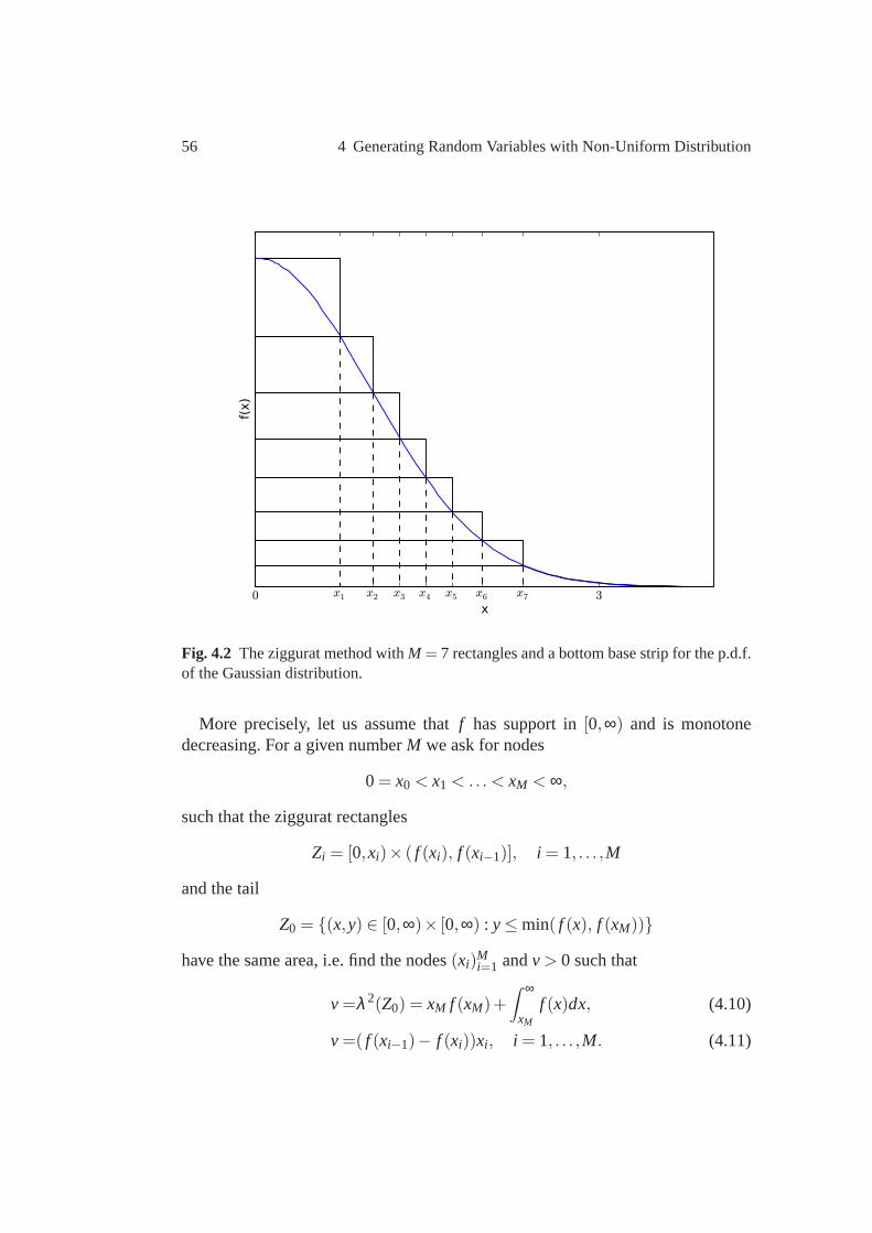
56 4 Generating Random Variables with Non-Uniform Distribution
0 x1 x2 x3 x4 x5 x6 x7 3x
f(x)
Fig. 4.2 The ziggurat method withM = 7 rectangles and a bottom base strip for the p.d.f.of the Gaussian distribution.
More precisely, let us assume thatf has support in[0,∞) and is monotonedecreasing. For a given numberM we ask for nodes
0= x0 < x1 < .. . < xM < ∞,
such that the ziggurat rectangles
Zi = [0,xi)× ( f (xi), f (xi−1)], i = 1, . . . ,M
and the tail
Z0 = (x,y) ∈ [0,∞)× [0,∞) : y≤ min( f (x), f (xM))
have the same area, i.e. find the nodes(xi)Mi=1 andv> 0 such that
v=λ 2(Z0) = xM f (xM)+∫ ∞
xM
f (x)dx, (4.10)
v=( f (xi−1)− f (xi))xi , i = 1, . . . ,M. (4.11)
4.4 Marsaglia’s Ziggurat Method 57
In Problem 4.10 we compute the nodes(xi)Mi=1 and v > 0 by using Newton’s
method.Then theZiggurat Method proceeds as follows:
1. Choosei ∈ 0, . . . ,M at random, uniformly distributed.2. GenerateU ∼U(0,1).3. If i ≥ 1 then
- Let X =Uxi.- If X < xi−1 then returnX,- else generateY ∼U(0,1) independent ofU .
If f (xi)+Y( f (xi−1)− f (xi))< f (X) then acceptX, otherwise reject.4. If i = 0 then
- SetX = vUf (xM) .
- If X < xM, acceptX,- else generate a random valueX ∈ [xM,∞) from the tail.
Note that in step 3 the conditionX < xi−1 holds in most cases. Then neither thesecond variableY is generated norf (X) is evaluated. The same remark applies tothe casei = 0. In that case a rectangle of areav and heightf (xM) has length v
f (xM) ,
henceX = vUf (xM) generates a random point on the base line of this rectangle that is
accepted ifX < xM. Otherwise one generates anX-value from the tail for whichdifferent methods are available (see below).
The efficiency of the method is determined by the quotient of the integral offand the area of the ziggurat
eff =(
λ 2(
M⋃
i=0
Zi
))−1=
1(M+1)v
. (4.12)
For the exponential p.d.f.f (x) = max(x,0)e−x the paper [26] gives the followingdata:
M = 255, xM = 7.697117470131104972,
eff = 0.989, v= 0.00394965598225815571993.
For the tail one generatesU1 ∼ U(0,1) and takesX = xM − log(U1) since then(compare with Example 4.2)
P(X ∈ [a,b]) = P(exM−b ≤U1 ≤ exM−a) =∫ b
aexM−xdx.
For the normal distribution one generates an additonal random sign± for thevalue ofX which is determined from the ziggurat method applied to the distribu-tion in [0,∞). For the nonnormalized density functionf (x) = exp(−x2
2 ) Marsagliaand Tsang [26] give the data
58 4 Generating Random Variables with Non-Uniform Distribution
M = 255, xM = 3.6541528853610088,
eff = 0.9933, v= 0.00492867323399 .
As a tail method they propose (see Problem 4.11)
1. GenerateU1 ∼U(0,1),U2 ∼U(0,1).2. SetX1 =− log(U1)
xM, X2 =− log(U2).
3. If X21 < 2X2 acceptX = xM +X1, otherwise reject.
For the implementation it is convenient to takeM = 2N −1 and to generate theindex i in step 1 and the valueU in step 2 from a random integerj ∈ 0, . . . ,2K −1 whereK > N. Typical values areN = 8,K = 32. In addition, one saves time byputting all operations withK-bit integers into the preparatory phase
ki ,wi =
⌊
2K xi−1xi
⌋
, 2−Kxi , i = 1, . . . ,2N −1,⌊
2K xM f (xM)v
⌋
, 2−K vf (xM) . i = 0.
(4.13)
With these settings the algorithm becomes rather short:
The Ziggurat Algorithm
1. Generate a random integerj ∈ 0, . . . ,2K −1 and determinei ∈ 0, . . . ,2N−1from the rightmostN bits of j.
2. SetX = jwi .3. If j < ki returnX, else
- If i = 0 return anX from the tail, else- if ( f (xi−1)− f (xi))U < f (X)− f (xi), returnX.
4. Go to step 1.
Exercises
Problem 4.6.The standardized logistic distribution has the density function
f (x) =exp(−x)
(1+exp(−x))2 , x∈ R.
Show how to use the inversion method to generate a random variable having thisdistribution.
Problem 4.7.Write a Matlab program with the following properties:
(i) Implement anN(0,1)-pseudo-random number generator which is based onthe inversion method and uses the Matlab functionserfinv andrand .

4.4 Marsaglia’s Ziggurat Method 59
(ii) Modify the idea of a quantile-quantile plot in such a waythat it can be usedto visualize if two pseudo-random number generators draw numbers from thesame distribution. Write a function which generates a quantile-quantile plot fortwo given sequences of random dataU = (U1, . . . ,UN) andV = (V1, . . . ,VN).
(iii) Produce a quantile-quantile plot which compares the distribution of theMatlab functionrandn versus your PRNG from (i).
Problem 4.8.Show that the first two steps of the algorithm in Example 4.4 gen-erate a random variable with p.d.f.g(x) = 1
2e−|x|. Set up an alternative algorithmwhich uses the inversion method instead. Compare the numerical efficiency ofboth methods.
Problem 4.9.In order to implement Marsaglia’s Ziggurat method one first needsto determine the nodes 0= x0 < x1 < .. . < xM < ∞ for a given numberM. Writea Matlab program which approximates the nodes in the following way: Solve thenonlinear equationg(xM) = 0 by using the bisection method, where the functiong: (0,∞)→ R is given by
g(xM) = v−x1(
f (x0)− f (x1))
,
with
v= xM f (xM)+∫ ∞
xM
f (x)dx,
xi−1 = f−1( vxi+ f (xi)
)
, i = M, . . . ,2.
Compute the nodes forM = 7, f (x) = e−12x2
and initial valuesx7 = 2.3 and 3.
Problem 4.10.Write a MATLAB program that uses Newton’s method to deter-mine the solutions(xi)
Mi=1 andv > 0 to the nonlinear system of equations (4.10)
and (4.11) forM = 7 and the normal distribution density function, that is
f (x) =1√2π
e−x22 .
Determine the efficiency of the ziggurat algorithm withM = 7.Hint: Reformulate (4.10) and (4.11) into the problem of finding the root ˜x ∈
RM+1 of a mappingF : RM+1>0 → RM+1, where
x=
x1...
xM
v
.
The implementation ofF may use the built-in functionerf .

60 4 Generating Random Variables with Non-Uniform Distribution
Problem 4.11 (Tail method for the Ziggurat algorithm). For xM > 0 considerthe algorithm
1. Generate independent random variablesU1 ∼U(0,1), U2 ∼U(0,1),2. SetX1 =− log(U1)
xM, X2 =− log(U2),
3. If X21 < 2X2 acceptX = xM +X1.
Show that this algorithm generates a random variableX whose distribution isgiven by the probability density function
f (x) =
0, x< xM
c−1exp(−12x2), x≥ xM,
with the constantc=∫ ∞
xMe−
12y2
dy.
Problem 4.12.Show that the Ziggurat algorithm is obtained from the general Zig-gurat method via the preparatory steps (4.13).
Chapter 5Monte Carlo Methods
The general termMonte Carlo Methodsrefers to numerical methods that use ran-dom numbers for conducting experiments on a computer. Roughly speaking onemay categorize Monte Carlo Methods into two different subclasses:
• Direct simulation of a random system;• Addition of artificial randomness into a given (deterministic) problem followed
by a simulation of the new system.
While our main goal, the numerical solution of stochastic differential equationsbelongs to the first category, we consider in this chapter a typical example fromthe second category: approximating definite integrals froma sequence of i.i.d.random variables. For example, it is quite natural to use theacceptance/rejectionmethod from Section 4.2 in order to estimate the area under the graph of thefunction f in Figure 4.1 (assuming we do not know thatf is a p.d.f.).
5.1 Statistical Analysis of Simulation Output
Let us first summarize basic results from statistical analysis that follow from thelaw of large numbers and the central limit theorem in Section2. Given a sequenceof i.i.d. random variablesXj , j = 1,2, . . . we want to estimate its expectation, thevariance, and a confidence interval. To be specific, letµ =E[Xj ] and var(Xj) = σ2
for j ∈ N. We estimate the expectationµ by thesample mean
XN =1N
N
∑j=1
Xj . (5.1)
From the Strong Law of Large Numbers (Theorem 2.12) we infer
XN → µ almost surely as N → ∞.
61
62 5 Monte Carlo Methods
By the linearity of the expectation,
E[XN] =1N
E[
N
∑j=1
Xj]
= µ,
and by the independence of theXj (see (2.7)),
var(XN) =1
N2
N
∑j=1
var(Xj) =1N
σ2.
Because of these propertiesXN is called aconsistent (or unbiased) estimator. Thusthe standard deviation ofXN is σ√
N. This decays at the rate1√
Nwhich dominates
the asymptotic behavior of practically all Monte Carlo simulations.The Central Limit Theorem 2.14 tells us that
(XN −µ)√
Nσ
→ N(0,1) in distribution. (5.2)
In order to use this for estimating how far our sample mean is from the expectedvalueµ, we compute an approximation ofσ2 from thesample variance
S2N =
1N−1
N
∑i=1
(Xi − XN)2. (5.3)
The valueSN is called thesample standard deviation. The following Lemmashows thatS2
N is an unbiased estimator of the true variance.
Lemma 5.1.Under the assumptions above the sample variance S2N has expecta-
tion E[S2N] = σ2.
Proof. First note that
S2N =
1N−1
N
∑i=1
(N−1N
Xi −1N ∑
j 6=i
Xj
)2
=1
(N−1)N2
N
∑i=1
(
(N−1)Xi −∑j 6=i
Xj
)2,
where(N−1)Xi −∑ j 6=i Xj is a sum of independent random variables which hasexpectation 0. Thus by (2.7) and (2.6),

5.1 Statistical Analysis of Simulation Output 63
E[S2N] =
1(N−1)N2
N
∑i=1
E[
(
(N−1)Xi −∑j 6=i
Xj)2]
=1
(N−1)N2
N
∑i=1
var(
(N−1)Xi −∑j 6=i
Xj)
=1
(N−1)N2
N
∑i=1
(
(N−1)2σ2+(N−1)σ2)= σ2.
⊓⊔Definition 5.2.Let Z be a random variable withZ ∼ N(0,1) and let 0< α < 1be given. Then the interval[−zα ,zα ] is called a 1−α confidence interval (or a100(1−α)% confidence interval) providedP(|Z| ≤ zα) = 1−α. The value ofαis referred to as thesignificance level.
Usually we think ofα being a small number, a common value in Statistics isα = 0.05. If f is the p.d.f. forN(0,1) thenzα can be computed from
1−α =∫ zα
−zαf (ξ )dξ = 2
∫ zα
−∞f (ξ )dξ −1,
i.e. by using a quantile from theN(0,1)-distribution. We evaluatezα numericallywith the help of the Matlab functionserf anderfinv , whereerf is given by
erf(x) :=2√π
∫ x
0e−t2
dt, for all x≥ 0, (5.4)
and, consequently,
zα =√
2erfinv(1−α), (5.5)
since
1−α = 2∫ zα
0f (ξ )dξ =
2√2π
∫ zα
0e−
12ξ 2
dξ = erf( zα√
2
)
.
For example,α = 0.05 leads tozα ≈ 1.96.We apply this toZN = (XN−µ)
√N
SNwhere we replace the unknown varianceσ2
in (5.2) by the sample varianceS2N from (5.3). Then we obtain forN large
1−α ≈ P(
|XN −µ|√
Nσ
≤ zα)
≈ P(
|XN −µ|√
NSN
≤ zα)
(5.6)
= P(
µ ∈[
XN −zαSN√
N, XN +zα
SN√N
])
.

64 5 Monte Carlo Methods
Therefore, we take
[
XN −zαSN√
N, XN +zα
SN√N
]
(5.7)
as our 100(1−α)% confidence interval . Note that the width of this interval ispro-portional to the sample standard deviation and inverse proportional to the squareroot of the number of samples.
Note that (5.6) involves two approximations:N should be so large that the Cen-tral Limit Theorem applies and such that our sample varianceis sufficiently accu-rate.
Example 5.3 ([14], Section 15.2).Consider the i.i.d. sequenceXj = exp(Z j) ob-tained from an i.i.d. sequenceZ j ∼ N(0,1). The expectation is
E[Xj ] =1√2π
∫
Rexp(x− 1
2x2)dx
=1√2π
∫
Rexp(−1
2(x−1)2+
12)dx=
√e.
We compute a Monte Carlo approximation ofµ = E[Xj ] by usingN = 2k,k =5, . . . ,17 samples. In Figure 5.1 the resulting valuesXN are plotted versusN (log-arithmic scale for both axes), the dashed line is at heightµ =
√e, and the 95%
confidence intervals (5.7) are indicated byerror bars.For the second example we return to the computation of the expected payoff
from (1.11).
Example 5.4 ([14], Section 15.3).Given a time horizonT > 0, volatility σ > 0,interest rater > 0, and initial valueS0 we compute the discounted expected payoff
V(S0) = exp(−rT )E [max(0,S(T)−E)] , where
S(T) = S0exp(
(r − 12
σ2)T +σ√
TZ)
andZ ∼ N(0,1). Here we again apply the risk neutrality assumptionµ = r.As in the previous example Figure 5.2 shows the values of the sample meanVN
together with the 95% confidence intervals computed from (5.7) for the data
T = 1, S0 = 10, E = 9, σ = 0.1, r = 0.06, N = 2k (k= 5, . . . ,17).
For comparison the dashed line gives the value of the Black-Scholes formula(1.10).
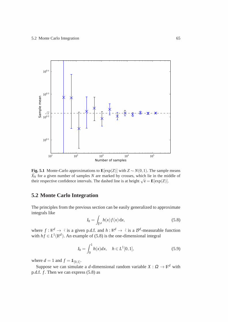
5.2 Monte Carlo Integration 65
101 102 103 104 105
Number of samples
100.1
100.2
100.3
100.4
√e
Sample m
ean
Fig. 5.1 Monte-Carlo approximations toE[exp(Z)] with Z ∼ N(0,1). The sample meansXN for a given number of samplesN are marked by crosses, which lie in the middle oftheir respective confidence intervals. The dashed line is at height
√e= E[exp(Z)].
5.2 Monte Carlo Integration
The principles from the previous section can be easily generalized to approximateintegrals like
Ih =∫
Rdh(x) f (x)dx, (5.8)
where f : Rd → R is a given p.d.f. andh : Rd → R is aBd-measurable functionwith h f ∈ L1(Rd). An example of (5.8) is the one-dimensional integral
Ih =∫ 1
0h(x)dx, h∈ L1[0,1], (5.9)
whered = 1 and f = 1[0,1].Suppose we can simulate ad-dimensional random variableX : Ω → Rd with
p.d.f. f . Then we can express (5.8) as
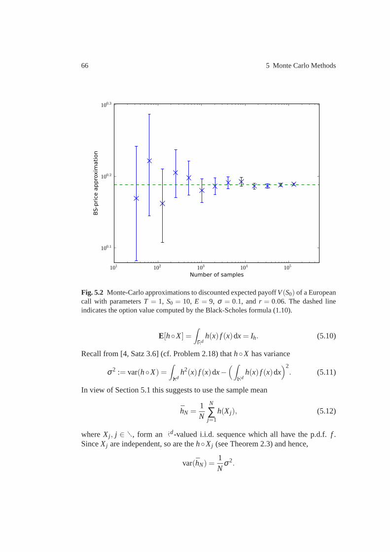
66 5 Monte Carlo Methods
101 102 103 104 105
Number of samples
100.1
100.2
100.3
BS-price
approxim
ation
Fig. 5.2 Monte-Carlo approximations to discounted expected payoffV(S0) of a Europeancall with parametersT = 1, S0 = 10, E = 9, σ = 0.1, andr = 0.06. The dashed lineindicates the option value computed by the Black-Scholes formula (1.10).
E[hX] =∫
Rdh(x) f (x)dx= Ih. (5.10)
Recall from [4, Satz 3.6] (cf. Problem 2.18) thathX has variance
σ2 := var(hX) =∫
Rdh2(x) f (x)dx−
(
∫
Rdh(x) f (x)dx
)2. (5.11)
In view of Section 5.1 this suggests to use the sample mean
hN =1N
N
∑j=1
h(Xj), (5.12)
whereXj , j ∈ N, form anRd-valued i.i.d. sequence which all have the p.d.f.f .SinceXj are independent, so are thehXj (see Theorem 2.3) and hence,
var(hN) =1N
σ2.

5.3 Variance Reduction Techniques 67
By the Law of Large Numbers, we have convergencehN → Ih almost surely. More-over, the Central Limit Theorem (Theorem 2.14) asserts
(hN − Ih)
√N
σ→ N(0,1) in distribution.
As in Section 5.1 we estimate the varianceσ2 by
S2N =
1N−1
N
∑i=1
(
h(Xi)− hN)2.
We then obtain a 100(1−α)% confidence interval from
P(
Ih ∈[
hN −zαSN√
N, hN +zα
SN√N
]
)
≈ 1−α (5.13)
wherezα is determined by (5.5).There are two important observations that we will discuss inthe following sub-
sections:
• While the convergence rate1√N
is unavoidable we can try to speed up the
process by transforming the integral (5.8) such that its varianceσ2 becomessmaller;
• The rate of convergence1√N
is independent of the dimensiond of the phasespace and of the smoothness of the integrand. This is in contrast to standardquadrature methods (trapezoidal sum, Romberg integration,Gauß-quadrature)and suggests that Monte Carlo methods are an alternative to classical methodsfor higher dimensions, see Section 5.4.
5.3 Variance Reduction Techniques
This section is based on [14, Ch.21] and [21, Ch.3]. A rather extensive treatmentunder the heading ofimportance samplingcan be found in [9, Ch. 6].
Variance reduction by antithetic variatesConsider the sample mean from (5.12)
hN =1N
N
∑j=1
h(Xj), Xj ∼U(0,1) (5.14)
for approximatingE[hX] =∫ 1
0 h(x)dx= Ih. We replacehN by the new antitheticsampler
68 5 Monte Carlo Methods
hN =1N
N
∑j=1
12
(
h(Xj)+h(1−Xj))
. (5.15)
Since the summands are independent we obtain from (2.7)
var(hN) =1
N2
N
∑j=1
var(1
2(h(Xj)+h(1−Xj))
)
.
Using var(X+Y) = var(X)+var(Y)+2cov(X,Y) ((2.8)) we can write
var(12(h(Xj)+h(1−Xj))) =
12
(
var(hXj)+cov(h(Xj),h(1−Xj)))
. (5.16)
Thus we have a reduction of variance if cov(h(Xj),h(1−Xj)) is negative, thesmaller the better. Assuming cov(h(Xj),h(1−Xj)) =−c2 we find
var(hN) =1
N2N12(σ2−c2) =
12N
(σ2−c2). (5.17)
According to (5.13) the width of the confidence interval improves by a factor of
ρ =(var(hN)
var(hN)
)1/2=√
2( σ2
σ2−c2
)1/2. (5.18)
The factor√
2 is natural since the antithetic sampler needs 2N function evalua-tions, so the improvement factor is σ√
σ2−c2 .The following theorem gives a sufficient criterion for two random variables to
have positive covariance.
Theorem 5.5.Let X be a random variable on(Ω ,F ,P) with values in a Borelset A⊂ R and let f,g ∈ L2(A,PX) be real-valued functions that are either bothincreasing or both decreasing. Then
cov(g(X),h(X))≥ 0. (5.19)
Proof. Let Y be another random variable which is independent ofX and has thesame distribution (for the existence see [4, Kor.9.5]). By the monotonicity as-sumption
(g(x)−g(y))(h(x)−h(y))≥ 0 for all x,y∈ A,
and hence by the independence ofh(X) andg(X) (compare Theorem 2.3),
0≤ E[(g(X)−g(Y))(h(X)−h(Y))]
= E[g(X)h(X)]−E[g(Y)h(X)]−E[g(X)h(Y)]+E[g(Y)h(Y)]
= 2(
E[g(X)h(X)]−E[g(X)]E[h(X)])
= 2cov(g(X),h(X)).
⊓⊔

5.3 Variance Reduction Techniques 69
Remark 5.6.There is a generalization of Theorem 5.5 tod variables that can beproved by induction ond, see [21, Theorem 3.17]. Consider anRd-valued randomvariableX = (X1, . . . ,Xd) with independent componentsXj that have values inBorel setsA j ⊂ R. Two square integrable functionsg,h : ∏d
j=1A j → R that aremonotone increasing with respect to each argument then satisfy (5.19).
The application of Theorem 5.5 to the antithetic sampler (5.15) is quite obvious:if h(x) is monotone increasing or decreasing on[0,1], then so is−h(1−x), hence
cov(h(Xj),h(1−Xj)) =−cov(h(Xj),−h(1−Xj))≤ 0.
Example 5.7.([14, Ch. 21.4])Let h(x) = e
√x,x∈ [0,1] andX ∼U(0,1). Then
E[h(X)] =∫ 1
0e√
xdx= 2
var(h(X)) =∫ 1
0e2
√xdx−4=
12(e2−7),
and
cov(e√
X,e√
1−X) = E[e√
X√
1−X]−E[e√
X]E[e√
1−X]
=∫ 1
0e√
x+√
1−xdx−4.
From (5.18) we obtain the factorρ = 13.463 by which the confidence intervalshould shrink. Table 5.1 shows the result of a Monte Carlo simulation with valuesN = 10i , i = 2,3,4,5. The last column gives the ratio of widths of confidenceintervals for the standard and the antithetic sampler whichis close to the predictedvalue.
Table 5.1 95%-Confidence Intervals for standard and antithetic MC-approximationsofE[e
√U ] = 2 with U ∼U(0,1).
N Standard Antithetic Ratio ofwidths
102 [1.85131,2.02127] [1.99413,2.00732] 12.887103 [1.96229,2.01589] [1.99945,2.00340] 13.563104 [1.99145,2.00886] [1.99899,2.00028] 13.535105 [1.99961,2.00508] [1.99966,2.00007] 13.433
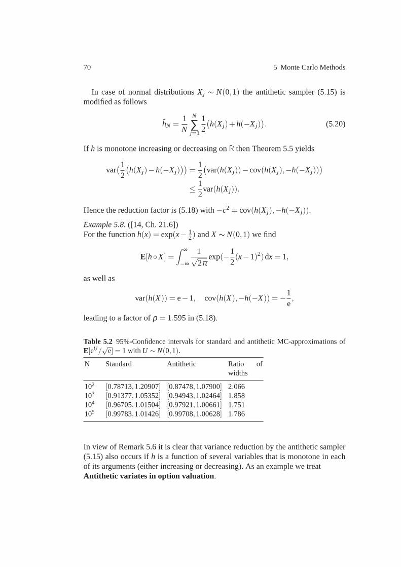
70 5 Monte Carlo Methods
In case of normal distributionsXj ∼ N(0,1) the antithetic sampler (5.15) ismodified as follows
hN =1N
N
∑j=1
12
(
h(Xj)+h(−Xj))
. (5.20)
If h is monotone increasing or decreasing onR then Theorem 5.5 yields
var(1
2
(
h(Xj)−h(−Xj)))
=12
(
var(h(Xj))−cov(h(Xj),−h(−Xj)))
≤ 12
var(h(Xj)).
Hence the reduction factor is (5.18) with−c2 = cov(h(Xj),−h(−Xj)).
Example 5.8.([14, Ch. 21.6])For the functionh(x) = exp(x− 1
2) andX ∼ N(0,1) we find
E[hX] =∫ ∞
−∞
1√2π
exp(−12(x−1)2)dx= 1,
as well as
var(h(X)) = e−1, cov(h(X),−h(−X)) =−1e,
leading to a factor ofρ = 1.595 in (5.18).
Table 5.2 95%-Confidence intervals for standard and antithetic MC-approximations ofE[eU/
√e] = 1 with U ∼ N(0,1).
N Standard Antithetic Ratio ofwidths
102 [0.78713,1.20907] [0.87478,1.07900] 2.066103 [0.91377,1.05352] [0.94943,1.02464] 1.858104 [0.96705,1.01504] [0.97921,1.00661] 1.751105 [0.99783,1.01426] [0.99708,1.00628] 1.786
In view of Remark 5.6 it is clear that variance reduction by theantithetic sampler(5.15) also occurs ifh is a function of several variables that is monotone in eachof its arguments (either increasing or decreasing). As an example we treatAntithetic variates in option valuation .

5.3 Variance Reduction Techniques 71
Consider an exotic option where the payoff function does not only depend on thefinal asset prizeS(T) but also on the intermediate values
S(t j), t j = j∆ t, ∆ t =TM, j = 0, . . . ,M.
For example, a barrierB > E is introduced and the payoff function (1.8) of theEuropean call is modified to
C((S(t j)Mj=0)) =
L if max j=0,...,M S(t j)> B,max(0,S(T)−E) otherwise.
If the threshold valueL equals zero then we have anup-and-out callwhereasL = B−E leads to alock-in call . If the asset prize passes the barrierB during thetime interval[0,T] then the payoff is set to zero or to the limit valueB−E. Weassume that asset prizes form a stochastic process generated by the solution (1.13)of the SODE (1.12)
S(t j+1) = S(t j)exp((r − 12
σ2)∆ t +σ√
∆ tZ j), Z j ∼ N(0,1), j = 0, . . . ,M−1.
(5.21)
Figure 5.3 shows a process that crosses the barrier and another one that doesn’t.Using the sameZ j from (5.21) we generate antithetic variates through
S(t j+1) = S(t j)exp((r − 12
σ2)∆ t −σ√
∆ tZ j), Z j ∼ N(0,1), j = 0, . . . ,M−1.
(5.22)
Figure 5.4 shows the corresponding zigzag and zagzig curves. PerformingN runs,indexed byi = 1, . . .N, we finally evaluate the discounted expected payoffs from
Vi = e−rT
L if max j=0,...,M Si(t j)> B,max(0,Si(T)−E) otherwise,
Vi = e−rT
L if max j=0,...,M Si(t j)> B,max(0, Si(T)−E) otherwise.
Note that the value function satisfies the monotonicity condition for the lock-incall L = B−E but not for the up-and-out callL = 0. Table 5.3 confirms thatantithetic variates give only a slight improvement over thefactor
√2≈ 1.414 for
the up-and-out call while the improvement for the lock-in-call is substantial, seeTable 5.4.
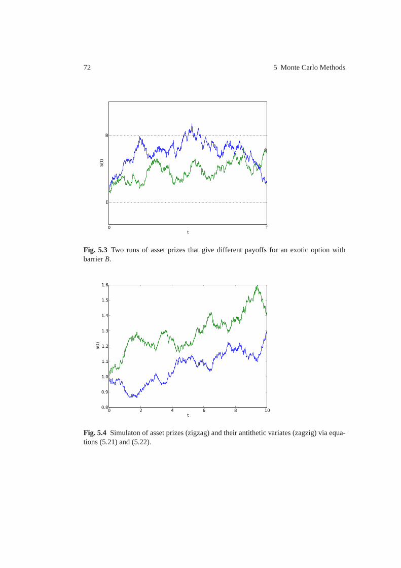
72 5 Monte Carlo Methods
0 Tt
E
B
S(t)
Fig. 5.3 Two runs of asset prizes that give different payoffs for an exotic option withbarrierB.
0 2 4 6 8 10t
0.8
0.9
1.0
1.1
1.2
1.3
1.4
1.5
1.6
S(t)
Fig. 5.4 Simulaton of asset prizes (zigzag) and their antithetic variates (zagzig) via equa-tions (5.21) and (5.22).

5.3 Variance Reduction Techniques 73
Table 5.3 95%-Confidence Intervals for MC-approximations of the discounted expectedpayoff of an Up-and-Out Call withS0 = 5, r = 0.05, σ = 0.3, E = 4, B = 8, T = 10,M = 500
N Standard Antithetic Ratio ofwidths
102 [0.48009,0.71627] [0.60471,0.73706] 1.785103 [0.54037,0.61606] [0.55460,0.60152] 1.613104 [0.58772,0.61197] [0.58889,0.60352] 1.658105 [0.59321,0.60091] [0.59450,0.59913] 1.661
Table 5.4 95%-Confidence Intervals for MC-approximations of the discounted expectedpayoff of an “Lock-in Call” withS0 = 5, r = 0.05,σ = 0.3,E= 4,B= 8,T = 10,M = 500
N Standard Antithetic Ratio ofwidths
102 [1.09702,1.67199] [1.14481,1.36578] 2.602103 [1.06575,1.22454] [1.13721,1.20512] 2.339104 [1.13987,1.19037] [1.15421,1.17543] 2.379105 [1.15785,1.17386] [1.16575,1.17251] 2.371
A note on importance sampling:
The Monte Carlo methods of Section 5.2 assume that the p.d.f.f ∈ L1(Rd)which occurs in the integral (5.8) is given. Suppose that this is not the case. Wewant to approximate an integral
∫
Rd hdx with h∈ L1(Rd) but still have a choice ofthe density function. Then we write
Ih =∫
Rdhdx=
∫
Rd
h(x)f (x)
f (x)dx, (5.23)
where f ∈ L1(Rd) is a p.d.f. to be determined such that
f (x) = 0, x∈ Rd =⇒ h(x) = 0. (5.24)
Let us defineh(x) = h(x)f (x) if f (x) 6= 0 andh(x) = 0 otherwise, and let us assume
that we can generate random variablesX ∼ f . Theimportance samplerthen reads
hN, f =1N
N
∑i=1
h(Xi) =1N
N
∑i=1
h(Xi)
f (Xi). (5.25)
It is natural to ask for a good choice of the density functionf that minimizes thevariance of this sampler.
74 5 Monte Carlo Methods
Theorem 5.9.The variance of the importance sampler(5.25)among all p.d.f.s fsatisfying(5.24)becomes minimal at
fmin(x) =|h(x)|‖h‖L1
, x∈ Rd, (5.26)
and the minimal value is
σ2( fmin) =(
∫
Rd|h(x)|dx
)2−(
∫
Rdh(x)dx
)2.
Remark 5.10.The theorem shows that it is optimal to choose as density the abso-lute value of the function itself (suitably normalized). Ofcourse, it is unrealisticto assume that one can generate random variables with this density. However, theresult suggests to look for densities that have some weight where the integrandhas. An example of this type of importance sampler will be discussed below.
Proof. Recall from (5.11) thatIh has variance
σ2( f ) =∫
Rd
h(x)2
f (x)dx−
∫
Rdh(x)2dx. (5.27)
Then our assertion follows from the equality
σ2( f ) = ‖h‖2L1E[
( fmin− ff
)2]
+‖h‖2L1 −
(
∫
Rdhdx)2.
The latter relation is obtained from (5.26) and (5.27) by a short calculation
‖h‖2L1E[
f 2min
f 2 −2fmin
f+1
]
=‖h‖2L1
∫
Rd
[
|h|2‖h‖2
L1 f 2−2
|h|‖h‖L1 f
+1
]
f dx
=∫
Rd
h2
fdx−2‖h‖2
L1 +‖h‖2L1.
⊓⊔
Finally we discuss a method of variance reduction calledStratified sampling.Consider again the integral (5.10) and the sample mean (5.12). Suppose that wecan decomposeRd into disjoint subsetsSi , i = 1, . . . ,M (thestrata) for which weknow conditional probabilities

5.3 Variance Reduction Techniques 75
ai =∫
Si
f (x)dx, i = 1, . . . ,M, Rd =
M⋃
i=1
Si , Si ∩Sj = /0 (i 6= j). (5.28)
Note that∑Mi=1ai = 1. With this information at hand we ask for an estimator ofIh
which has smaller variance thanhN. Note that (5.28) implies a decomposition ofthe density functionf as follows
f =M
∑i=1
ai fi , where fi(x) = 1Si(x)f (x)ai
, x∈ Rd.
We decompose the number of samplesN = ∑Mi=1ni and assume that we can gen-
erate i.i.d. random variablesXi,1, . . . ,Xi,ni ∈ Si such thatXi, j ∼ fi . Then the samplemean in stratumSi is given by
Ti =1ni
ni
∑j=1
h(Xi, j),
and ourstratified sampleris defined by
T =M
∑i=1
aiTi . (5.29)
A simple computation shows
E[Ti] =Iiai, where Ii =
∫
Si
h(x) f (x)dx, (5.30)
E[T] =M
∑i=1
aiE[Ti] = Ih. (5.31)
For the variance we find
var(T) =M
∑i=1
a2i var(Ti) =
M
∑i=1
a2i
ni
(
∫
Si
h2(x)f (x)ai
dx−( Ii
ai
)2). (5.32)
Theorem 5.11.In the setting above let ni = Nai , i = 1, . . . ,M be integers, then thevariance of the sample mean(5.12)and the stratified mean(5.29)satisfy
var(hN) = var(T)+1N
M
∑i=1
ai( Ii
ai− Ih
)2. (5.33)
76 5 Monte Carlo Methods
Remark 5.12.The choiceni = Nai is calledproportional allocation. In general,one cannot assume thatni = Nai are integers. Then one takes nearby values suchthatN = ∑M
i=1ni still holds. Equation (5.33) shows that the variance is reduced byproportional allocation and that the reduction is better the further apart the valuesof E(Ti) andIh are.
Proof. By (5.32) and the choice ofni the right-hand side of (5.33) equals
M
∑i=1
a2i
1aiN
(
∫
Si
h2 fai
dx−( Ii
ai
)2)+
1N
M
∑i=1
( I2i
ai−2IiIh+aiI
2h
)
=1N
M
∑i=1
∫
Si
h2(x) f (x)dx−2I2h
N+
I2h
N= var(hN).
⊓⊔
Example 5.13.([21, Ch.3.2])Suppose you askN Bielefeld residents whether their city mayor is doing a goodjob. For simplicity think of each resident to represent an interval of length 1 andlet R(x) denote the resident of the interval to whichx belongs. You then considerthe sample meanhN = 1
N ∑Ni=1h(xi) of the function
h(x) =
1 if R(x) says yes,0 if R(x) says no.
We stratify the set of residents by
Si = x : R(x) votes for partyi, i = 1, . . . ,6,
where i stands for SPD, CDU, GRUNE, FDP, LINKE, OTHER. From the lastelection we know the proportionai =
1B
∫
Si1dx of residents (B total number of
voters) that voted for partyi. Suppose you also ask theN residents how they votedduring the last election and you obtain numbersni for the i-th party. Suppose44.2% of them voted SPD while you know from the newspapers that wehad onlya1 = 0.396 during the last election. You may then worry about the result of yoursample mean because you probably have too many SPD-voters inyour sampleand the SPD is the mayor’s party. Therefore you decide to extract from yourN-sample a proportional allocation by taking the answers of ˜ni = Nai ≤ ni votersxi, j
of partyi such thatN= ∑6i=1 ni ≤N (note thatN=min ni
aiis the maximum number
for doing this). Then the stratified estimate of the mayor’s supporters is
T =6
∑i=1
aiTi , Ti =1ni
ni
∑j=1
h(xi, j).
5.3 Variance Reduction Techniques 77
The following theorem shows that proportional allocation is not the best choicefor minimizing the variance of the stratified sampler.
Theorem 5.14.(Tschuprow-Neyman allocation)The variance of the stratified sampler(5.29)is minimal for
nopti = N
aiσi
∑Mj=1a jσ j
, σi = var(h(Xi, j)), j = 1, . . . ,ni, (5.34)
and the minimal value is
var(Topt) =1N
(
M
∑j=1
a jσ j)2.
Proof. From (5.32) we infer for a general decompositionN = ∑Mi=1ni
V(n1, . . . ,nM) := var(T) =M
∑i=1
a2i
σ2i
ni.
An application of the Cauchy Schwarz inequality yields the assertion
V(nopt1 , . . . ,nopt
M ) =1N
(
M
∑j=1
a jσ j)2
=1N
(
M
∑j=1
√n j
a jσ j√n j
)2 ≤ 1N
(
M
∑j=1
n j)(
M
∑j=1
a2j σ2
j
n j
)
=V(n1, . . . ,nM).
⊓⊔
It is known that the Cauchy Schwarz inequality is strict unless the vectors arelinearly dependent, i.e.
√n j = c
a j σ j√n j
for somec∈ R. Since∑Mj n j = N this leads
to n j = noptJ , hence (5.34) is the unique allocation where the minimum is attained.
In general it is hard to achieve this minimum since one needs to know the stratavariancesσ2
i . Moreover,nopti need not be integers in general. A practical way out
is to start sampling with proportional allocation and then estimateσ2i from the
sample variance
S2N,i =
1Nai
ni
∑j=1
(h(Xi, j)−Ti)2.
One may then use the allocation (5.34) withSN.i instead ofσi and continue withincreasing the sample size.

78 5 Monte Carlo Methods
5.4 Approximation of Multiple Integrals
This section is based on [9], [10, Ch. 7.1], [30, Ch. 4.3]. We first review quadraturerules for one-dimensional integrals, with an emphasis on Gaussian quadrature forweight functions that are probability density functions. Then we show how to gen-eralize to multiple integrals via product rules. Finally wecompare the efficiencyof these quadrature rules with Monte-Carlo integration.
The general goal is to approximate an integral
I(h) =∫
Ah(x) f (x)dx, A⊂ R
d measurable (5.35)
with a p.d.f. f ∈ L1(A) by aquadrature ruleof the form
QM(h) =M
∑i=1
wih(xi), wherex1, . . . ,xM ∈ A. (5.36)
We callxi ∈ A thenodesandwi ∈ R theweightsof the quadrature rule.In the following we assumeA⊂R and the nodes to be ordered byx1 < .. . < xM.
LetPM−1 denote the space of polynomials of degree≤M−1. The following resultabout interpolatory quadrature is well known (the proof is an exercise).
Theorem 5.15.The quadrature rule(5.36) is exact for polynomials inPM−1 (i.e.QM(h) = I(h) for all h ∈ PM−1) if and only if the weights are given by
wi =∫
Aℓi(x) f (x)dx, i = 1, . . . ,M, (5.37)
with the Lagrange polynomials defined by
ℓi(x) =M
∏j=1, j 6=i
x−x j
xi −x j.
For equidistant nodesx j = a+( j −1)∆x, j = 1, . . . ,M with A= [a,b],∆x= b−aM−1
we obtain the Newton-Cotes formulae. The most familiar ones are
Q2(h) =b−a
2
(
h(a)+h(b))
, trapezoidal rule, (5.38)
Q3(h) =b−a
6
(
h(a)+4h(a+b
2)+h(b)
)
, Simpson’s rule. (5.39)
For Gauß quadrature rules consider an intervalA⊂ R (not necessarily compact)and the function space
5.4 Approximation of Multiple Integrals 79
L2f (A) = h : A 7→ R measurable andh2 f ∈ L1(A).
Assumingf > 0 a.e. inA, the spaceL2f (A) is a Hilbert space (cf. Section 2.3) with
respect to
〈h,g〉=∫
Ah(x)g(x) f (x)dx, ‖h‖2 = 〈h,h〉.
From the monomialsmj(x) = x j , j = 0, . . . ,M−1 one generates orthogonal poly-nomialsPi ∈ Pi by the Gram-Schmidt orthogonalization process
Pi = mi −i−1
∑j=0
〈mi ,Pj〉〈Pj ,Pj〉
Pj , i = 0, . . . ,M−1. (5.40)
Rather than normalizing〈Pi ,Pi〉= 1 the recursion (5.40) enforces the leading coef-ficient to be 1, i.e.Pi(x) = xi + l .o.t.. We callPi , i ∈ N theorthogonal polynomialsassociated with the weight function f and the interval A. Using this property it iseasy to verify that orthogonal polynomials satisfy a three term recursion.
Theorem 5.16.The orthogonal polynomials associated with the weight functionf and the interval A satisfy the recursion
Pi+1(x) = (x−ai+1)Pi(x)−bi+1Pi−1(x), i ≥ 0,
ai+1 =〈m1Pi ,Pi〉〈Pi ,Pi〉
, bi+1 =〈m1Pi ,Pi−1〉〈Pi−1,Pi−1〉
,
where we set P−1 ≡ 0,P0 ≡ 1,b1 = 0.
From this we conclude important information about the zeroes of the orthogonalpolynomials.
Theorem 5.17.Let the orthogonal polynomials be defined by(5.40). Then Pi hasexactly i distinct zeroes in the interior of A.
Proof. Let z1, . . . ,zν be the zeroes ofPi in the interior ofA repeated accordingto their multiplicity. We haveν ≤ i sincePi ∈ Pi. Then the polynomialQi(x) =Pi(x)∏ν
l=1(x−zl ) is of one sign in the interior ofA and hence
0 6=∫
AQi(x) f (x)dx=
∫
APi(x)
ν
∏l=1
(x−zl ) f (x)dx.
If ν < i then this integral vanishes due to the orthogonality〈Pi ,Pl 〉 = 0 forl < i. Hence we concludeν = i. Now assume that there is a zero of multi-plicity k ≥ 2, say z1. Then we can repeat the above argument withQi(x) =Pi(x)(x−z1)
k−2∏il=2(x−zl ) and arrive at a contradiction. ⊓⊔

80 5 Monte Carlo Methods
Definition 5.18.Let
x1,M < .. . < xM,M (5.41)
denote the distinct zeroes ofPM in A and let
wi,M =∫
Aℓi,M(x) f (x)dx, ℓi,M(x) =
M
∏j=1, j 6=i
x−x j,M
xi,M −x j,M, i = 1, . . . ,M (5.42)
be the corresponding Lagrangian weights (cf. (5.37)). Thenthe quadrature rule
QM(h) =M
∑i=1
wi,Mh(xi,M) (5.43)
is called theM-th Gaussian rule associated with domain A and density f.
Theorem 5.19.The M-th Gaussian rule associated with domain A and density fis exact for polynomials inP2M−1, i.e.
QM(h) =∫
Ah(x) f (x)dx for all h∈ P2M−1.
Proof. Forh∈P2M−1 let P[h] = ∑Mi=1h(xi,M)ℓi,M ∈PM−1 be its interpolating poly-
nomial. By Theorem 5.17 there exists somer ∈ PM−1 such that
h(x) = P[h](x)+ r(x)PM(x), x∈ R.From this factorization and the orthogonality we obtain
I(h) =∫
AP[h](x) f (x)dx+ 〈r,PM〉
= I(P[h]) = QM(P[h]) =M
∑i=1
wi,MP[h](xi,M)
=M
∑i=1
wi,M(
P[h](xi,M)+ r(xi,M)PM(xi,M))
= QM(h).
⊓⊔The favorable properties of Gaussian quadrature rules allow for a rather simpleconvergence proof asM → ∞.
Theorem 5.20.The weights of the M-th Gaussian rule satisfy
wi,M > 0 (i = 1, . . .M),M
∑i=1
wi,M = 1. (5.44)
If A is a compact interval then one has convergence
limM→∞
QM(h) =∫
Ah(x) f (x)dx for all h∈C(A). (5.45)
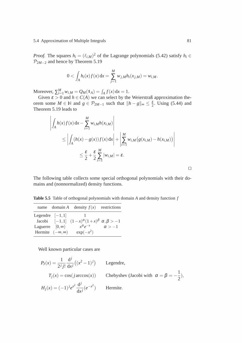
5.4 Approximation of Multiple Integrals 81
Proof. The squareshi = (ℓi,M)2 of the Lagrange polynomials (5.42) satisfyhi ∈P2M−2 and hence by Theorem 5.19
0<∫
Ahi(x) f (x)dx=
M
∑j=1
w j,Mhi(x j,M) = wi,M.
Moreover,∑Mi=1wi,M = QM(1A) =
∫
A f (x)dx= 1.Givenε > 0 andh∈C(A) we can select by the Weierstraß approximation the-
orem someM ∈ N and g ∈ P2M−1 such that‖h− g‖∞ ≤ ε2. Using (5.44) and
Theorem 5.19 leads to∣
∣
∣
∣
∣
∫
Ah(x) f (x)dx−
M
∑i=1
wi,Mh(xi,M)
∣
∣
∣
∣
∣
≤∣
∣
∣
∣
∫
A(h(x)−g(x)) f (x)dx
∣
∣
∣
∣
+
∣
∣
∣
∣
∣
M
∑i=1
wi,M(
g(xi,M)−h(xi,M))
∣
∣
∣
∣
∣
≤ ε2+
ε2
M
∑i=1
|wi,M|= ε.
⊓⊔
The following table collects some special orthogonal polynomials with their do-mains and (nonnormalized) density functions.
Table 5.5 Table of orthogonal polynomials with domainA and density functionf
name domainA density f (x) restrictions
Legendre [−1,1] 1Jacobi [−1,1] (1−x)α(1+x)β α ,β >−1
Laguerre [0,∞) xαe−x α >−1Hermite (−∞,∞) exp(−x2)
Well known particular cases are
PJ(x) =1
2 j j!d j
dx j
(
(x2−1) j) Legendre,
Tj(x) = cos( j arccos(x)) Chebyshev (Jacobi withα = β =−12),
H j(x) = (−1) jex2 d j
dx j (e−x2
) Hermite.
82 5 Monte Carlo Methods
Error estimatesAs noted above classical integration rules aim at accurate integration of suffi-
ciently smooth functions. Approximating smooth functionsby a Taylor expansionthen suggests to set up quadrature rules that integrate polynomials exactly to thehighest degree possible. For an extensive treatment of error estimates asM → ∞we refer to the classical monographs of Davis, Rabinowitz [7]and Stroud [33].Here we draw some simple conclusions that follow from the results above.
Theorem 5.21.Let A⊂ R be a compact interval and consider a quadrature ruleQM as in(5.36)that is exact for polynomials inPM−1. Then for all h∈CM(A),
|I(h)−QM(h)| ≤C1,M‖h(M)‖L∞ , C1,M =1
M!
∫
A
M
∏i=1
|x−xi| f (x)dx. (5.46)
Proof. Let P[h] ∈PM−1 interpolate the data(xi ,h(xi)), i = 1, . . . ,M. For everyx∈Athere exists someξ = ξ (x) ∈ (x1,xM) such that
h(x)−P[h](x) =h(M)(ξ )
M!ωM(x), ωM(x) =
M
∏i=1
(x−xi). (5.47)
With this representation we find from Theorem 5.15
|I(h)−QM(h)|= |∫
A(h(x)−P[h](x)) f (x)dx|
≤ ‖h(M)‖L∞
M!
∫
A|ωM(x)| f (x)dx.
⊓⊔For the Gauss rules with respect to domainA and densityf the corresponding
result is the following.
Theorem 5.22.Let A⊂R be a compact interval and consider a Gaussian quadra-ture rule(5.43)associated with domain A and density f . Then for all h∈C2M(A),
|I(h)−QM(h)| ≤C2,M‖h(2M)‖L∞ , C2,M =1
(2M)!
∫
A
M
∏i=1
(x−xi)2 f (x)dx.
(5.48)
Proof. We modify the proof of Theorem 5.21 by lettingP[h] ∈ P2M−1 solve theHermite interpolation problem
P[h](xi,M) = h(xi,M), P′[h](xi,M) = h′(xi,M), i = 1, . . . ,M.
Then the error formula (5.47) holds with 2M andω2M instead ofM andωM, and
the estimate (5.48) follows as in the previous proof. ⊓⊔

5.4 Approximation of Multiple Integrals 83
Compound rulesOne way of increasing the accuracy of quadratrure rules is topartition the do-
main of integration into smaller subdomains and to use a simple rule on each sub-domain. In this way one obtains so calledcompound rules. In one dimension theresulting formulae integrate exactly continuous and piecewise polynomial func-tions (splines). Note however, that this approach usually requires the density to beconstant, for otherwise we will need a new quadrature rule oneach subdomain.
Let A= [a,b] and f (x) = 1,x∈ [a,b] and partition as follows
[a,b] =K−1⋃
j=0
[y j ,y j+1], y j = a+ j∆x, j = 0, . . . ,K, ∆x=b−a
K.
We apply a formula (5.36) for∫ 1
0 hdx to the functionsg j(y) = h(y j + y∆x),y ∈[0,1], j = 0, . . . ,K−1,
∫ b
ah(x)dx=
K−1
∑j=0
∫ y j+1
y j
h(x)dx= ∆xK−1
∑j=0
∫ 1
0g j(y)dy
≈ ∆xK−1
∑j=0
QM(g j) = ∆xK−1
∑j=0
M
∑i=1
wih(y j +xi∆x) =: QM,K(h). (5.49)
Theorem 5.23.Under the assumptions of Theorem 5.21 the compound quadraturerule QM,K defined in(5.49)satisfies for all h∈CM(A)
|I(h)−QM,K(h)| ≤C1,M(b−a)(∆x)M‖h(M)‖L∞ . (5.50)
For the compound Gaussian rules we have under the assumptionsof Theorem 5.22
|I(h)−QM,K(h)| ≤C2,M(b−a)(∆x)2M‖h(2M)‖L∞ . (5.51)
Proof. We consider only the first case, the second case is treated analogously.From (5.46) we obtain
|I(h)−QM,K(h)|=|∆xK−1
∑j=0
(
∫ 1
0g j(y)dy−QM(g j)
)
|
≤∆xK−1
∑j=0
C1,M‖g(M)j ‖‖L∞
≤∆xC1,M
K−1
∑j=0
(∆x)M‖h(M)‖L∞
=(b−a)C1,M(∆x)M‖h(M)‖L∞ .
⊓⊔
84 5 Monte Carlo Methods
A simple compound rule is the trapezium sum that derives fromthe trapezoidalrule (5.38)
Q2,K(h) = ∆x(1
2h(a)+
K−1
∑j=1
h(a+ j∆x)+12
h(b))
. (5.52)
This is anO((∆x)2) approximation of the integral ifh∈C2[a,b].
Product rules
Exercises
Problem 5.24.Let X be a random variable withX ∼U(0,1). Compute the expec-tation and the variance of
hα(X) =(
X−α)2
for 0≤ α ≤ 1. For the valuesα ∈ 0, 12,1 discuss whether antithetic sampling of
hα(X) reduces the variance.
Problem 5.25.The acceptance-rejection algorithm of Section 4.2 can be modifiedto produce a Monte-Carlo integrator for
Ih =∫
Rdh(x)dx, h∈ L1(Rd).
Assume|h(x)| ≤ c f(x),x∈ Rd, for some p.d.f.f ∈ L1(Rd). For i = 1, . . . ,N gen-erate independent random variablesYi ∼U(0,c) andUi ∼ f and set
hN =cN
N
∑i=1
Xi , where Xi =
1, if Yi f (Ui)< h(Ui),
−1, if Yi f (Ui)<−h(Ui),
0, otherwise.
Show thathN has expectationIh and variance1N
(
c||h||L1 − I2h
)
. Show that the im-portance sampler
hN =1N
N
∑i=1
h(Zi)
f (Zi), where Zi ∼ f
has the same expectation but smaller variance.
Problem 5.26.Implement the following Monte-Carlo algorithm which approxi-mates the Delta∆(t) of a European call option with exercise priceE > 0 andexpiry dateT > 0 at timet = 0:
5.4 Approximation of Multiple Integrals 85
1. Fori ∈ 1, . . . ,N generateZi ∼ N(0,1) i.i.d.2. Fori ∈ 1, . . . ,N compute
Si := S0exp(
(r − 12
σ2)T +σ√
TZi)
and for a given step sizeη > 0
Sηi := (S0+η)exp
(
(r − 12
σ2)T +σ√
TZi)
.
3. Compute∆i =1η e−rT
(
max(0,Sηi −E)−max(0,Si −E)
)
4. Compute the sample mean∆N = 1N ∑N
i=1∆i .
As parameter values useT = 3, E = 5, S0 = 6, r = 0.05,σ = 0.3. For the numberof samples chooseN = 25, . . . ,217 and for the step sizes setη = 10−2, . . . ,10−4.For eachη make a separate error bar plot which shows the exact value of∆(0)and the approximations∆N for the given number of samplesN together with their95%-confidence intervals.
Problem 5.27.Let X be a real-valued random variable with unknown expectationand letY be a random variable with known expectation. Determine the expectationand variance of
Xθ = X+θ(
E[Y]−Y)
, for θ ∈ R.
How would you chooseθ in order to minimize the variance when samplingXθand what is its minimal value? Generalize this to the case ofk random variablesYj , j = 1, . . . ,k, by minimizing the variance of
Xθ = X+k
∑j=1
θ j(
E[Yj ]−Yj)
with θ = (θ1, . . . ,θk) ∈ Rk. Give a criterion that guarantees a unique minimizer.
Problem 5.28.Determine the interpolatory quadrature rule withM ∈2,3 equidis-tant nodes for
I(h) =∫ 1
0h(x) f (x)dx,
where f (x) = 6x(1− x). Determine nodes and weights for the correspondingGauß-rules withM ∈ 1,2 nodes.

86 5 Monte Carlo Methods
Problem 5.29.A fixed strike lookback calloption has the payoff function
Λ((S(t j))Mj=0) = max
(
maxj=0,...,M
S(t j)−E,0)
, t j = j∆ t,∆ =TM, j = 0, . . . ,M.
The stochastic processS(t j) is determined in the usual way through
S(t j+1) = S(t j)exp((r − 12
σ2)∆ t−σ√
∆ tZ j), Z j ∼ N(0,1), j = 0, . . . ,M−1.
Write a program which calculates the 95%-confidence intervals for the standardand the antithetic Monte-Carlo approximations of the discounted expected payoffof the option. Present your results in a table together with the ratio of widths.
Take parameter valuesT = 10, M = 500, r = 0.05, σ = 0.3, S(0) = S0 = 5,E = 4 and generateN = 102, . . . ,105 samples.

Chapter 6Theory of Continuous Time Stochastic Processes andIt o-Integrals
6.1 Continuous Time Stochastic Processes
In this section we introduce basic notions of the theory of continuous time stochas-tic processes. In particular, we deal with filtrations, adaptiveness of stochastic pro-cesses and stopping times. For the material presented in this section our mainreferences are [22, Sec. 1.3] and [34, Ch. 2].
Throughout this section let(Ω ,F ,P) be the underlying probability space.
Definition 6.1.A family (X(t))t∈T, T ⊂ [0,∞), of random variables with valuesin Rd is called astochastic processwith index setT and state spaceRd. Wesay that a stochastic process isintegrable(square-integrable) if X(t) ∈ L1(Ω ;Rd)(X(t) ∈ L2(Ω ;Rd)) for all t ∈ T.
Forω ∈ Ω the mappingT ∋ t 7→ X(t,ω) ∈ Rd is called asample pathor trajec-tory of the stochastic process.
Although most definitions and results also make sense for discrete index setsT, for the rest of this chapter we takeT to be equal to a bounded or unboundedsubinterval of[0,∞). In this case we say that we consider a stochastic process incontinuous time– in contrast to adiscrete timestochastic process.
We say that a stochastic process(X(t))t∈T is continuousif the mappingsT ∋t 7→ X(t,ω) ∈ Rd are continuous for almost everyω ∈ Ω . In a similar way, wedefine a stochastic process(X(t))t∈T to be left continuousor right continuous.Further, we say that a stochastic process iscadlag (French: “continuea droite,limite a gauche”) if it is right continuous and the left limits limsրt X(s,ω) existsfor almost everyω ∈ Ω .
Next, we introduce a very important concept which is used to control the evo-lution of information in a stochastic system.
Definition 6.2.A family of sub-σ -algebras(Ft)t∈T ⊂ F is called afiltration ifFs ⊂Ft for all s≤ t.
87
88 6 Theory of Continuous Time Stochastic Processes and Ito-Integrals
Theσ -algebraFt should be regarded as the set of all events for which we candecide at timet whether they have occurred or not. An important example of afiltration is the so callednatural filtrationof a stochastic process(X(t))t∈T whichis defined by
Ft := σ(X(s) : s∈ T,s≤ t), t ∈ T,
that is,Ft is the smallestσ -algebra for which the random variablesX(s), s≤ t,are measurable.
Definition 6.3.A stochastic process(X(t))t∈T is called adaptedto a filtration(Ft)t∈T if the random variablesX(t) areFt-measurable for everyt ∈ T.
Clearly, the smallest filtration to which a stochastic process X is adapted is itsnatural filtration. A useful enlargement of the natural filtration is given by the nextdefinition.
Definition 6.4.For a given filtration(Ft)t∈T consider
F+t :=
⋂
ε>0
Ft+ε
for everyt ∈ T. We say that the filtration(Ft)t∈T is right-continuousif Ft = F+t
for all t ∈ T.
From the definition it follows at once thatFt ⊂F+t and that(F+
t )t∈T is a right-continuous filtration.
We are also interested in stopping a stochastic process if given random eventsoccur. For example, we may sell a certain stock if the stock price hits a prescribedbarrier. For this it is important that the decision to stop attime t only depends onthose information which are available at timet. This is formalised in the followingdefinition.
Definition 6.5.Consider a filtration(Ft)t∈T and a random variableτ : Ω → T∪∞. We say thatτ is an(Ft)t∈T-stopping timeif τ ≤ t ∈ Ft for all t ∈ T.
Obviously, a constant random variable is a stopping time. For right-continuousfiltrations the following characterization holds true (c.f. [34, Lemma 2.2.2]).
Lemma 6.6.Let (Ft)t∈T be a right-continuous filtration. A random variableτ : Ω → T∪ ∞ is a (Ft)t∈T-stopping time if and only ifτ < t ∈ Ft for allt ∈ T.

6.1 Continuous Time Stochastic Processes 89
Proof. For the proof we follow [34, Lemma 2.2.2]. First we assume that τ < t ∈Ft for all t ∈ T. Then it follows that
τ ≤ t=∞⋂
n=1
τ < t +1n
∈∞⋂
n=1
Ft+ 1n= F+
t = Ft for all t ∈ T.
Conversely, letτ be a stopping time. Thus
τ < t
=∞⋃
n=1
τ ≤ t − 1n
∈ Ft ,
sinceFt− 1n⊂Ft for all n≥ 1 with t − 1
n ∈ T. In addition, ift0 := inf(T) ∈ T, then
τ < t0= /0∈ Ft0. ⊓⊔
Next, we come to an important example of a stopping time.
Definition 6.7.Let (X(t))t∈T be anRd-valued stochastic process and letD be asubset ofRd. Then the random variableτD : Ω → T∪∞ which is given by
τD(ω) := inf
t ∈ T : X(t,ω) /∈ D
,
with the usual convention inf /0= ∞, is called the(first) exit timeof X from D.
We have the following result (c.f. [22, Th. 1.3.2] and [34, Prop. 2.3.4]).
Lemma 6.8.Let (Ft)t∈T be a right-continuous filtration and(X(t))t∈T an Rd-valued, (Ft)t∈T-adapted stochastic process. If(X(t))t∈T is left-continuous orright-continuous then the exit timeτD of X from a closed subset D⊂ Rd is an(Ft)t∈T-stopping time.
Proof. Following the proof of [34, Prop. 2.3.4], we have
τD < t
=⋃
s<t
X(s) ∈ Dc=⋃
s<t,s∈Q
X(s) ∈ Dc,
which belongs toFt by the adaptiveness ofX. The last equality holds sinceDc
is open andX is left-continuous or right-continuous. Therefore, ifX(s) /∈ D forsomes< t then there also exists ˜s∈ Q, s< t, with X(s) ∈ Dc.
By applying Lemma 6.6 the proof is complete. ⊓⊔
We close this section with what is known as the “usual conditions” in the liter-ature (c.f. [34, Sec. 2.1])
Assumption 6.9.Let (Ω ,F ,P) be a probability space together with a filtration(Ft)t∈T which satisfies the followingusual conditions:

90 6 Theory of Continuous Time Stochastic Processes and Ito-Integrals
(i) (Ω ,F ,P) is a complete probability space, that is, every subsetA⊂ N of aP-nullsetN is F-measurable.
(ii) Every P-nullsetN ∈ F also belongs toFt for all t ∈ T.(iii) The filtration (Ft)t∈T is right-continuous.
Throughout the rest of these lecture notes we usually assumethat Assumption6.9 is satisfied if not stated otherwise.
6.2 Martingales
In this section we consider an important class of stochasticprocesses, the so calledmartingales. Historically, martingales have been introduced by Paul Pierre Levy,while many important results of this theory were contributed by Joseph Leo Doob.
The name is related to a betting system with the simplest variant working inthe following way: Imagine a game of flipping a fair coin. The gambler’s stakeis doubled if the coin comes up heads, otherwise the stake is completely lost.The betting strategy asks the gambler to double his stake after every loss. Thenthe reward of the first win after a streak of several losses equals the sum of allprevious losses plus a gain of the initial stake.
However, due to the exponential growth of the stakes during along sequence ofconsecutive losses the gambler might hit its credit limit and the strategy results inthe gambler’s bankruptcy. This potentially catastrophic loss, which occurs with asmall but strictly positive probability, results in the fact that the overall expectedreturn is equal to zero.
In probability theory a martingale can be seen as a fair game.A consequenceof Doob’s optional stopping theorem is that there exist no betting system whichprovides a positive expected return in a fair game. For a moredetailed discussionin this direction we refer to [4,§17] and [5, Sec. 35].
In the following we review some aspects of the martingale theory which willprove useful later on. The presented material is standard and is found in, for ex-ample, [34, Ch. 3]. For the following definition we recall the notion of conditionalexpectation from Section 2.6.
Definition 6.10.Let (Ft)t∈T be a filtration. An adapted, real-valued, integrablestochastic process(X(t))t∈T is called amartingalewith respect to(Ft)t∈T if
E[X(t)|Fs] = X(s) for all s≤ t. (6.1)
If (6.1) only holds with ‘≥’ (‘ ≤’) then(X(t))t∈T is called asubmartingale(super-martingale).
6.2 Martingales 91
In the following section we will introduce Brownian motion which is an impor-tant stochastic process. The first part of Example 6.11 givesthe arguments whyBrownian motion is a martingale. The second part is a more artificial example.
Example 6.11.(i) Let (X(t))t∈T be an adapted, real-valued, integrable stochasticprocess such that the incrementsX(t)−X(s) are independent ofFs with E[X(s)] =E[X(t)] for all s< t.
Here, we say that a random variableY is independent of aσ -algebraG ⊂ F ifeveryG-measurable random variable is independent ofY. In particular, for 0≤t1 < t2 ≤ t3 < t4 < ∞ it follows that the incrementsX(t2)−X(t1) andX(t4)−X(t3)are independent.
In order to show the martingale property the following fact on conditional ex-pectation is needed
E[Y|G]≡ E[Y], (6.2)
which holds for all integrable random variablesY which are independent of asub-σ -algebraG. Using this, we compute
E[X(t)|Fs] = E[X(t)−X(s)|Fs]+E[X(s)|Fs] = E[X(t)−X(s)]+X(s) = X(s).
It remains to show (6.2), that is∫
AYdP=
∫
AE[Y]dP|G for all A∈ G.
Indeed, we have∫
AYdP= E[1AY] = E[1A]E[Y] = P(A)E[Y] =
∫
AE[Y]dP|G ,
since1A is a G-measurable random variable and thus independent ofX. Thisproves (6.2).
(ii) Consider a real-valued random variableX ∈ L1(Ω) and a filtration(Ft)t∈T.Then the process(X(t))t∈T defined by
X(t) := E[X|Ft ] for all t ∈ T
is a martingale. In fact, by the properties of the conditional expectation it holdsthat(X(t))t∈T is an adapted integrable process and
E[X(t)|Fs] = E[E[X|Ft ]|Fs] = E[X|Fs] = X(s) for all s≤ t.
⊓⊔

92 6 Theory of Continuous Time Stochastic Processes and Ito-Integrals
As our first lemma shows we often encounter submartingales asthe concatena-tion of a martingale and a convex function. An important application of this resultis ϕ(x) = |x|.Lemma 6.12.Consider a convex functionϕ : R→ R and a real-valued martin-gale (X(t))t∈T such thatϕ(X(t)) is integrable for all t∈ T. Then the process(ϕ(X(t)))t∈T is a submartingale.
Proof. As in the proof of [34, Lemma 3.0.16] we apply Jensen’s inequality forconditional expectations which yields
ϕ(X(s)) = ϕ(
E[X(t)|Fs])
≤ E[
ϕ(X(t))|Fs]
for all s≤ t. ⊓⊔Next, we are concerned with the regularity of typical samplepaths of a mar-
tingale. For this, we say that a stochastic process(Y(t))t∈T is amodificationof astochastic process(X(t))t∈T if P(X(t) =Y(t)) = 1 for all t ∈ T.
Theorem 6.13.Under the usual conditions on(Ft)t∈T every martingale has acadlag modification.
A proof is found in [34, Th. 3.2.6 (ii)].A consequence of Doob’s martingale stopping theorem ([34, Th. 3.2.7]) is that
the martingale property remains valid after stopping the process by a stoppingtime.
Theorem 6.14.Consider a right-continuous (sub-)martingale(Xt)t∈T and a stop-ping timeτ. Then the stopped process(X(t ∧ τ))t∈T is also a (sub-)martingale.
For a proof we refer to [34, Cor. 3.2.8].The next result is the continuous version of Doob’s submartingale inequality.
The presented formulation is taken from [22, Th. 1.3.7]. A proof can be found in[34, Th. 3.2.10].
Lemma 6.15.Let p> 1and consider a real-valued nonnegative and right-continuoussubmartingale(X(t))t∈T such that X(t) ∈ Lp(Ω). Then it holds that
E[
sups≤t
X(s)p]≤( p
p−1
)pE[
X(t)p] for all t ∈ T.
Finally, we say that anRd-valued stochastic process is a martingale if all com-ponents are real-valued martingales. Note that all presented results also hold inthe multidimensional case. In particular, we have the following generalization ofLemma 6.12:
6.3 Brownian Motion 93
Lemma 6.16.Let (X(t))t∈T be anRd-valued martingale with respect to a filtra-tion (Ft)t∈T. If ϕ : Rd → R is a convex function andϕ(X(t)) is integrable for allt ∈ T, then(ϕ(X(t))t∈T is a real-valued submartingale with respect to(Ft)t∈T.
The proof is similar to the proof of Lemma 6.12 but uses a suitable generalizedversion of Jensen’s inequality for convex functions inRd.
6.3 Brownian Motion
In 1826–27 Robert Brown discovered what today is known as theBrownian mo-tion: Under the microscope he noticed that pollen particles suspended in watermove erratically. In particular, he saw that the path of a single particle seems to benowhere differentiable and that the paths of two particles appear to be independentof each other. As it was explained later, the Brownian motion is caused by a largenumber of collisions between the pollen particles and the molecules of water.
In his PhD-thesis from 1900 Louis Bachelier introduced a firstmathematicalmodel to describe fluctuations in stock prices using stochastic analysis. In 1905Albert Einstein studied the Brownian motion and used his results to give an indi-rect proof of the existence of atoms and molecules.
These findings resulted in a rigorous mathematical theory for the Brownianmotion which was first developed by Norbert Wiener during the1920’s. To hishonour the stochastic process which describes the physicalphenomena known asBrownian motion is also often called aWiener process.
Definition 6.17.A (standard)Wiener processor a (standard)Brownian motionisa real-valued continuous stochastic process(W(t))t∈T onT= [0,∞), adapted to afiltration (Ft)t∈T, which satisfies the following properties:
(i) W(0) = 0 a.s.;(ii) the incrementsW(t)−W(s) for 0≤ s< t < ∞ are normally distributed with
mean zero and variancet −s, that isW(t)−W(s)∼ N(0, t −s);(iii) the incrementsW(t)−W(s) are independent ofFs for all 0≤ s< t < ∞.
For a discussion of property (iii) we refer to Example 6.11 and Figure 6.1 showsa typical sample path of a Wiener process. But before we continue to study someimportant properties we present a motivation of the definition from [8, Ch. 3]which follows the way Albert Einstein studied Brownian motion.
If we inject a unit amount of ink at positionx= 0 and at timet = 0 into a longthin tube filled with water then letu(x, t) denote the density of ink at timet ≥ 0and at positionx∈ R. Thus, at timet = 0 the density is given by
u(x,0) = δ0(x), theδ -distribution centered at 0.
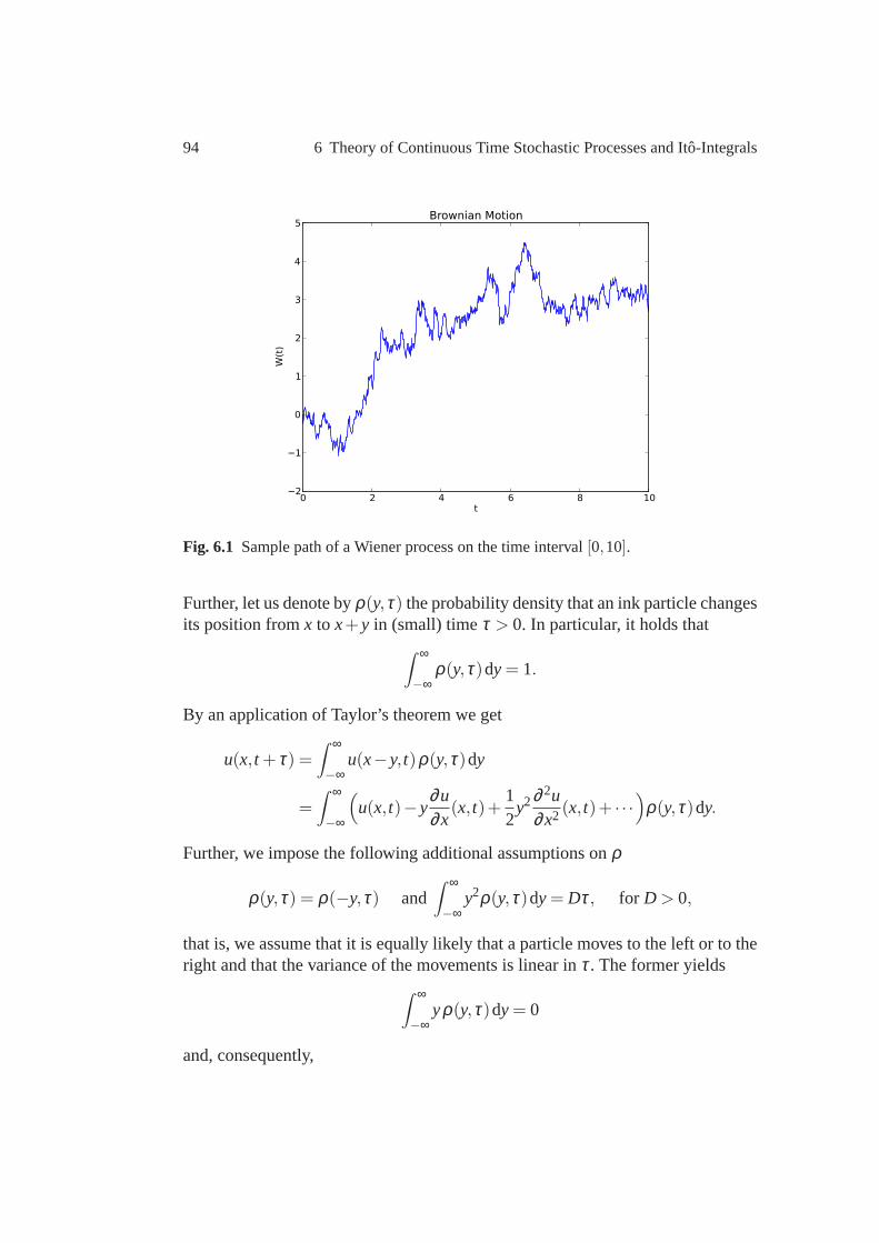
94 6 Theory of Continuous Time Stochastic Processes and Ito-Integrals
0 2 4 6 8 10t
−2
−1
0
1
2
3
4
5
W(t
)
Brownian Motion
Fig. 6.1 Sample path of a Wiener process on the time interval[0,10].
Further, let us denote byρ(y,τ) the probability density that an ink particle changesits position fromx to x+y in (small) timeτ > 0. In particular, it holds that
∫ ∞
−∞ρ(y,τ)dy= 1.
By an application of Taylor’s theorem we get
u(x, t + τ) =∫ ∞
−∞u(x−y, t)ρ(y,τ)dy
=∫ ∞
−∞
(
u(x, t)−y∂u∂x
(x, t)+12
y2∂ 2u∂x2 (x, t)+ · · ·
)
ρ(y,τ)dy.
Further, we impose the following additional assumptions onρ
ρ(y,τ) = ρ(−y,τ) and∫ ∞
−∞y2ρ(y,τ)dy= Dτ, for D > 0,
that is, we assume that it is equally likely that a particle moves to the left or to theright and that the variance of the movements is linear inτ. The former yields
∫ ∞
−∞yρ(y,τ)dy= 0
and, consequently,

6.3 Brownian Motion 95
1τ(
u(x, t + τ)−u(x, t))
=12
∂ 2u∂x2 (x, t)+ . . . .
Finally, the limitτ → 0 leads to the partial differential equation
∂u∂ t
=D2
∂ 2u∂x2 ,
u(x,0) = δ0(x),(6.3)
which is usually referred to as theheat equationor diffusion equation. The (fun-damental) solution to (6.3) is given by
u(x, t) =1√
2πDtexp(
− x2
2Dt
)
, (6.4)
which is the p.d.f. ofN(0,Dt). Since we started with a unit amount of ink we mayinterpretu as the probability density of the distribution of the ink particles.
Concerning the constantD, Albert Einstein computed
D =RTNA f
,
whereR is the gas constant,T the absolute temperature,f the friction coeffi-cient andNA denotes Avogadro’s number (≡ 6×1023 = number of molecules ina mole).
To sum up, in an idealized situation withD = 1 the new position at timet > 0of an ink particle which started atx= 0 isN(0, t)-distributed.
A further motivation of this result is given by the Central Limit Theorem. If wefollow the assumption that changes to the position of an ink particle are due toa large number of independent collisions with water molecules this will result innormally distributed position changes. A more rigorous derivation of this result,which also uses the Central Limit Theorem can also be found in [8, Sec. 3].
Before we discuss some useful properties of Wiener processeswe first notethat from Definition 6.17 it is not immediately clear if thereeven exists such astochastic process. The first existence result was presented by Norbert Wiener in1923. The following formulation of an existence theorem is found in [8, Ch. 3].
Theorem 6.18.Let (Ω ,F ,P) be a probability space on which a sequence(Zi)∞i=1
of countably many independent and N(0,1)-distributed random variables exists.Then there exists a filtration(Ft)t∈T with T = [0,∞) and an adapted stochasticprocess(W(t))t∈T such that W is a standard Wiener process.
For an easy-to-access proof of this theorem which relies on the Levy-Ciesielskiconstruction of a Wiener process we also refer to [8, Ch. 3] (which in turn gives[18] as a reference).
96 6 Theory of Continuous Time Stochastic Processes and Ito-Integrals
As it is discussed in [22, Sec. 15] the filtration(Ft)t∈T is part of the definitionof a Wiener process. The filtration which is given by Theorem 6.18 does usuallynot satisfy the usual conditions. But since this is often a convenient property weremark that if(W(t))t∈T is a Wiener process on a probability space(Ω ,F ,P) thenit is also a Wiener process on(Ω ,F ,P), whereF denotes the completion ofF(see (2.1)).
Further, ifN denotes the set of allP-null sets, that isN = A∈F : P(A) = 0,then we define
F t := σ(
Ft ∪N)
.
Clearly, (F t)t∈T is again a filtration to which(W(t))t∈T is adapted. This filtra-tion is called theaugmentation underP of (Ft)t∈T and, by a possibly further en-largement to(F+
t )t∈T we may also assume that it is right-continuous. Therefore,without loss of generality we may assume that(W(t))t∈T is a Wiener process withrespect to a filtration(Ft)t∈T which satisfies the usual conditions.
Our first lemmas are direct consequences of Definition 6.17. Byproperty (iii)in the definition of Wiener processes and the arguments givenin Example 6.11Brownian motion is a martingale.
Lemma 6.19.Let (W(t))t∈T, T = [0,∞), be a Wiener process with filtration(Ft)t∈T. Then(W(t))t∈T is a square-integrable(Ft)t∈T-martingale.
For weak convergence of numerical schemes it will be important that we can cal-culate the mean of observables that depend on the Brownian motion.
Lemma 6.20.Let (W(t))t∈T, T= [0,∞) be a Wiener process. Consider a measur-able function h: Rn → R with n≥ 0 and a choice of time points0= t0 < t1 < .. . <tn. Then we have
E[h(W(t1), . . . ,W(tn))] =∫
R· · ·∫
Rh(x1, . . . ,xn) f (x1;0, t1)×
f (x2;x1, t2− t1) · · · f (xn;xn−1, tn− tn−1)dx1 · · · dxn,
where
f (x;y, t) =1√2πt
e−(x−y)2
2t
denotes the density of a Gaussian random variable with mean y∈ R and variancet > 0.
6.3 Brownian Motion 97
Proof. Here we follow [8, Ch. 3, pp. 37 –38]. First we define
h(y1, . . . ,yn) = h(y1,y1+y2, . . . ,y1+ · · ·+yn),
then it holds
h(W(t1), . . . ,W(tn)) = h(W(t1),W(t2)−W(t1), . . . ,W(tn)−W(tn−1)).
Since the incrementsW(ti)−W(ti−1), i = 1, . . . ,n are independent it follows
E[h(W(t1),W(t2)−W(t1), . . . ,W(tn)−W(tn−1))]
=∫
Rnh(y1, . . . ,yn) f (y1;0, t1) f (y2;0, t2− t1) · · · f (yn;0, tn− tn−1)dy1 · · · dyn
=∫
Rnh(x1, . . . ,xn) f (x1;0, t1) f (x2;x1, t2− t1) · · · f (xn;xn−1, tn− tn−1)dx1 · · · dxn
where we used the transformationyi = xi − xi−1, i = 1, . . . ,n, with x0 = 0 forthe last equality. Note that the determinant of the Jacobianof this transformationequals 1. ⊓⊔
Further, the temporal regularity of Wiener processes playsan important rolesince this determines the order of convergence of the numerical schemes whichwe study later.
Lemma 6.21.Let (W(t))t∈T, T= [0,∞), be a Wiener process. Then we have
E[
|W(t)−W(s)|p]
=C|t −s| p2
for all real numbers p≥ 1, t,s∈ T and a constant C> 0 only depending on p.
Proof. Assume thatt ≥ s. SinceW(t)−W(s) ∼ N(0, t − s) we get for thep-thmoment
E[
|W(t)−W(s)|p]
=2
p2 Γ ( p+1
2 )√π
(t −s)p2 .
Thus, the assertion follows by setting
C :=2
p2 Γ ( p+1
2 )√π
.
⊓⊔
The previous lemma provides information on the temporal regularity of (W(t))t∈Twith respect to theLp-norm. Together with the following famous theorem we canuse this result to analyze the temporal continuity of typical sample paths.

98 6 Theory of Continuous Time Stochastic Processes and Ito-Integrals
Theorem 6.22 (Kolmogorov-Chentsov).Let (X(t))t∈T, T = [0,∞), be anRd-valued stochastic process such that there existsα,β > 0 and C> 0 with
E[
|X(t)−X(s)|α]
≤C|t −s|1+β for all s, t ∈ T.
Then there exists a modification(X(t))t∈T of (X(t))t∈T such that every samplepath t 7→ X(t,ω), ω ∈ Ω , is locally Holder continuous for each exponent0< γ <βα , that is, for every T> 0, ω ∈ Ω there exists a constant K(T,γ,ω) such that
|X(t,ω)− X(s,ω)| ≤ K|t −s|γ for all 0≤ s, t ≤ T.
A proof of this theorem is found in [4, Kor. 39.5] or in [8, p. 47].In the following we often assume the existence of a Wiener process with con-
tinuous sample paths. This is justified by the next corollary.
Corollary 6.23. Let (W(t))t∈T, T= [0,∞), be a Wiener process. Then there existsa modification of(W(t))t∈T of (W(t))t∈T such that every sample path t7→W(t,ω),ω ∈ Ω , is locally Holder continuous for each exponent0< γ < 1
2.
Proof. For p≥ 1 setα = 2p andβ = p−1. Then by Lemma 6.21 we get
E[
|W(t)−W(s)|α]
=C|t −s|1+β .
and Theorem 6.22 yields the existence of a modification(W(t))t∈T of (W(t))t∈Tsuch that every sample path of(W(t))t∈T is locally Holder continuous for eachexponent 0< γ < β
α . Sincep≥ 1 is arbitrary and
βα
=p−12p
=12− 1
2p
the assertion follows for each exponent 0< γ < 12. ⊓⊔
The regularity result from Corollary 6.23 can not be improvedas our next the-orem shows. In fact, a typical sample path of a Wiener processis nowhere differ-entiable. Following an idea of [5, p. 504] we provide an indication for this.
Let (W(t))t∈T be a Wiener process. Then Problem 6.36 (ii) (withc = N ∈ N)asks the reader to confirm that also the transformed process
WN(t) := N−1W(N2t)
is a Wiener process. For everyε > 0 there existN ≫ 1 large enough such that

6.3 Brownian Motion 99
P(
W(n)−W(n−1)> 1 for somen= 1, . . . ,N)
> 1− ε.
Now fix a sample pathω ∈ Ω andn= 1, . . . ,N such thatW(n,ω)−W(n−1,ω)>1 and note that an possible enlargement ofN does not affect our choice ofn andω. Then it holds that
W(n)−W(n−1) = N(
WN( n
N2
)
−WN(n−1
N2
)
)
=1N
WN(
nN2
)
−WN(
n−1N2
)
nN2 − n−1
N2
,
or equivalently,
WN(
nN2 ,ω
)
−WN(
n−1N2 ,ω
)
nN2 − n−1
N2
= N(
W(n,ω)−W(n−1,ω))
.
Therefore, the above difference quotient of the Wiener processWN exceedsN onthe short time interval[0, 1
N ], where we can chooseω from a set with probability1− ε. In particular, by lettingN → ∞ and sinceW andWN are identically dis-tributed for allN, it is equally likely to observe an arbitrarly large difference quo-tient in a sample path ofW on everyarbitrarly small time interval. This stronglycontradicts with the behaviour of differentiable functions.
In order to formulate the next result we recall that a mappingY : [a,b]→ R issaid to havebounded variationon the interval[a,b], if
Vba (Y) := sup
πn∑
tni ∈πn
∣
∣Y(tni )−Y(tn
i−1)∣
∣< ∞, (6.5)
where the supremum is taken over the set of allpartitions πn = a = tn0 < tn
1 <.. . < tn
Mn= b. Themesh sizeof πn is denoted by|πn|= max1≤i≤Mn |tn
i − tni−1|.
Theorem 6.24.Let (W(t))t∈T, T = [0,∞), be a Wiener process with continuoussample paths. For every12 < γ ≤ 1 the sample paths t7→ W(t,ω) are nowherelocally Holder continuous with exponentγ.
On the other hand, let(πn)n∈N be a sequence of partitions of[a,b] with |πn|→ 0for n→ ∞ andπn ⊂ πn+1 for all n ∈ N. Then the quadratic variation of a typicalsample path is given by
〈W〉[a,b] := limn→∞
Mn
∑i=1
(
W(tni )−W(tn
i−1))2
= b−a in L2(Ω). (6.6)
In particular, the sample paths are nowhere differentiable and have unboundedvariation on any finite interval[a,b]⊂ R.

100 6 Theory of Continuous Time Stochastic Processes and Ito-Integrals
0 2 4 6 8 10t
0
2
4
6
8
10
quadratic variation
Quadratic variation of Brownian motion
T/N = 0.10000T/N = 0.00100T/N = 0.00001
Fig. 6.2 Quadratic variation of a sample path of a Wiener process on the time interval[0,10].
Remark 6.25.The limit in (6.6) also convergesP-a.s. This is demonstrated in Fig-ure 6.2 which shows for one sample path of a Wiener process on[0,T] with T = 0the time evolution of the quadratic variation. More precisely, for the figure we usedthe equidistant partitionsπN = tN
i = i TN : i = 0, . . . ,N with N = 102,104,106.
Then the figure shows a sample path of the mappings
t 7→ ∑tNi ∈πNtNi <t
(
W(tNi )−W(tN
i−1))2 → t asN → ∞.
Proof (of Theorem 6.24).We only prove the last part of the theorem. For a proofof the first part we refer to [8, pp. 50–51].
In order to prove the assertion on the quadratic variation wefollow [8, p. 57]and for the partitionπn we set
Qn :=Mn
∑i=1
(W(tni )−W(tn
i−1))2.
Then we get
Qn− (b−a) =Mn
∑i=1
[
(W(tni )−W(tn
i−1))2− (tn
i − tni−1)
]
=:Mn
∑i=1
Yi,
6.3 Brownian Motion 101
whereE[Yi] = 0. It follows
E[
(Qn− (b−a))2]=Mn
∑i=1
E[Y2i ]+2
Mn
∑i, j=1i< j
E[YiYj ].
Note thatYj and Yi are independent fori 6= j and, consequently,E[YiYj ] =E[Yi]E[Yj ] = 0. Further, we have
E[Y2i ] = E
[((W(tni )−W(tn
i−1)√
tni − tn
i−1
)2−1)2]
(tni − tn
i−1)2
=1√2π
∫ ∞
−∞(x2−1)2e−
x22 dx(tn
i − tni−1)
2 = 2(tni − tn
i−1)2,
since
W(tni )−W(tn
i−1)√
tni − tn
i−1∼ N(0,1).
Therefore,
E[
(Qn− (b−a))2]= 2Mn
∑i=1
(tni − tn
i−1)2 ≤ 2|πn|(b−a),
which goes to zero asn → ∞. This proves theL2-convergence of the quadraticvariation to(b−a). In particular, by going to a subsequenceN′ ⊂ N we also getfor almost everyω ∈ Ω that
Mn
∑i=1
(W(tni ,ω)−W(tn
i−1,ω))2 → b−a asn→ ∞, n∈ N′.
Then for 0< γ < 12
0< b−a= limsupn→∞
Mn
∑i=1
|W(tni ,ω)−W(tn
i−1,ω)|2
≤ limsupn→∞
CMn
∑i=1
|tni − tn
i−1|γ |W(tni ,ω)−W(tn
i−1,ω)|
≤ limsupn→∞
C|πn|γMn
∑i=1
|W(tni ,ω)−W(tn
i−1,ω)|.
Thus, if a typical sample path of the Wiener process were of bounded variationthen this implies that the right hand side goes to zero. This contradiction provesthat sample paths of Wiener processes are of unbounded variation and, conse-quently, nowhere differentiable. ⊓⊔

102 6 Theory of Continuous Time Stochastic Processes and Ito-Integrals
−6 −5 −4 −3 −2 −1 0 1x1
−5
−4
−3
−2
−1
0
1
2
x2
Brownian motion trajectory in 2D
Fig. 6.3 Trajectory of the sample path of a two-dimensional Wiener process on the timeinterval[0,10].
So far, we considered Brownian motion only as a real-valued process. We con-clude this section with a generalization toRd.
Definition 6.26.An Rd-valued stochastic process
(W(t))t∈T = (W1(t), . . . ,Wd(t))t∈T
is ad-dimensional Wiener processonT= [0,∞) if it holds that
(i) each componentWi, i = 1, . . . ,d, is a real-valued Wiener process onT and(ii) the components are independent.
Figure 6.3 shows the trajectory of a sample path of a two-dimensional Wienerprocess. All results on the time regularity remain valid in thed-dimensional case.For the quadratic variation we get
〈W〉[a,b] = limn→∞
Mn
∑i=1
|W(tni )−W(tn
i−1)|2 = d(b−a), (6.7)
where| · | denotes the Euclidean norm inRd.
Remark 6.27.Here is a remark on “white noise” missing...
6.4 The Ito-Integral 103
6.4 The Ito-Integral
In this section we mainly follow [29, Sec. 2.3] and [22, Sec. 1.5]. Our aim is todefine the stochastic integral
∫ t
0h(s)dW(s), t ≥ 0, (6.8)
with respect to anRd-valued Wiener process(W(t))t∈T, T = [0,∞). We also pro-vide a characterization of the class of admissible integrands which will consists ofm×d-matrix valued stochastic processesh: T×Ω → Rm,d.
As we learned in the previous section (see Theorem 6.24) typical sample pathsof a Wiener process are of unbounded variation. Therefore, the integral in (6.8)cannot be defined in the usual sense of a Lebesgue-Stieltjes-integral.
In 1949 Kiyoshi Ito was the first who gave a meaningful definition of (6.8) usingcertain Riemann sums. Since then it is usually called thestochastic Ito-integral.
In the whole section let(Ω ,F ,P) denote a complete probability space. Further,let (W(t))t∈T be anRd-valued Wiener process with continuous sample paths andadapted to a filtration(Ft)t∈T which satisfies the usual conditions. We also fix atime T > 0.
Following [29, Sec. 2.3] the construction of the stochasticintegral is done inseveral steps:
Step 1: First we specify a classE of elementary stochastic processes which takevalues in the setRm,d. Then we define the integral for this class of integrands,that is, we define a mapping
Int : E →M2([0,T])
h 7→∫ t
0h(s)dW(s), t ∈ [0,T].
Here M2([0,T]) := M2([0,T];Rm) denotes the set of continuous, square-integrable,Rm-valued(Ft)-martingales. Below we show that this space is aBanach space.
Step 2: There exists a norm onE such that Int :E →M2([0,T]) is an isometry.Therefore, by using an extension theorem we can uniquely extend the domainof Int to the completionE .
Step 3: It remains to provide an explicit representation ofE .
Concerning the first step we begin with the definition of the elementary pro-cesses.
Definition 6.28.An Rm,d-valued stochastic process(h(t))t∈[0,T] is calledelemen-tary if there exists a partition 0= t0 < .. . < tn = T of [0,T], n∈ N, such that
104 6 Theory of Continuous Time Stochastic Processes and Ito-Integrals
h(t) =n−1
∑j=0
h j1(t j , t j+1](t), t ∈ [0,T], (6.9)
whereh j : Ω → Rm,d is Ft j -measurable for 0≤ j ≤ n−1 and only takes a finitenumber of values inRm,d.
By E we denote the set of all elementary processes.
Note that from (6.9) it follows directly that every elementary process is left-continuous. However, the representation (6.9) is not unique in general.
In the same way as in [29, Sec. 2.3.2] we define the mapping Int :E →M2([0,T]) by
Int(h)(t) :=∫ t
0h(s)dW(s) :=
n−1
∑j=0
h j(
W(t j+1∧ t)−W(t j ∧ t))
(6.10)
for everyt ∈ [0,T], whereh is an elementary process with representation 6.9. Asthe next lemma shows by this setting Int :E →M2([0,T]) is well-defined.
Lemma 6.29.Let h∈ E . Then the stochastic process(Int(h)(t))t∈[0,T] given by(6.10) is a continuous, square-integrable(Ft)t∈[0,T]-martingale which takes val-ues inRm. The mappingInt : E →M2([0,T]) is well-defined in the sense that itsdefinition does not depend on the particular representationof h.
Proof. In Problem 6.39 we ask the reader to confirm that the definition(6.10) isindependent of the representation ofh∈ E . For the rest of the proof we follow [29,Prop. 2.3.2].
For every representation ofh∈ E it directly follows that the mapping
t 7→∫ t
0h(s)dW(s) =
n−1
∑j=0
h j(
W(t j+1∧ t)−W(t j ∧ t))
is continuous for almost everyω ∈ Ω by the continuity of the Wiener process andsince the multiplication of the matrixh j(ω) ∈ Rm,d with the increment vector ofthe Wiener process is also continuous for allω ∈ Ω , 0≤ j ≤ n−1.
Next, since eachh j : Ω → Rm,d only takes a finite number of values it is clearthat supω∈Ω |h j(ω)| < ∞ for every 0≤ j ≤ n−1, where in this case| · | denotesthe matrix norm inRm,d which is induced by the Euclidean norms inRm andRd.Hence,
∣
∣h j(
W(t j+1∧ t)−W(t j ∧ t))∣
∣≤ |h j |∣
∣W(t j+1∧ t)−W(t j ∧ t)∣
∣
is square-integrable for every 0≤ j ≤ n−1, and, consequently, Int(h)(t) is square-integrable for everyt ∈ [0,T].

6.4 The Ito-Integral 105
Now, for t = 0 we haveh(0)≡ 0 which is obviouslyF0-measurable. For a fixedt ∈ (0,T] consider the indexi ∈ 0, . . . ,n−1 with ti < t ≤ ti+1. Then we get
Int(h)(t) =i−1
∑j=0
h j(
W(t j+1)−W(t j))
+hi(
W(t)−W(ti))
,
which is aFt-measurable random variable and, therefore,(Int(h)(t))t∈[0,T] isadapted.
It remains to prove the martingale property. For this we take0≤ s< t ≤ T anda setA∈ Fs arbitrarily. Then we have
E[
1A Int(h)(t)]
=n−1
∑j=0
E[
1Ah j(
W(t j+1∧ t)−W(t j ∧ t))]
. (6.11)
If we consider all summands with index 0≤ j ≤ n−1 such thatt j+1 < s then weget
E[
1Ah j(
W(t j+1∧ t)−W(t j ∧ t))]
= E[
1Ah j(
W(t j+1∧s)−W(t j ∧s))]
.
Further, for all summands with index 0≤ j ≤ n− 1 such thats≤ t j the incre-ment(W(t j+1∧ t)−W(t j ∧ t)) is independent of1Ah j ∈ Ft j sinceA∈ Fs ⊂ Ft j .Therefore, we obtain
E[
1Ah j(
W(t j+1∧ t)−W(t j ∧ t))]
= E[
1Ah j]
E[
W(t j+1∧ t)−W(t j ∧ t)]
= 0.
For the remaining summand with indexj ∈ 0, . . . ,n−1 such thatt j < s≤ t j+1
we have
E[
1Ah j(
W(t j+1∧ t)−W(t j ∧ t))]
= E[
1Ah j(
W(t j+1∧ t)−W(t j+1∧s))]
+E[
1Ah j(
W(t j+1∧s)−W(t j ∧s))]
and the first term again vanishes by the independence ofW(t j+1∧ t)−W(t j+1∧s)and1Ah j ∈ Fs = Ft j+1∧s. Altogether, we get for (6.11)
E[
1AInt(h)(t)]
=n−1
∑j=0
E[
1Ah j(
W(t j+1∧s)−W(t j ∧s))]
= E[
1AInt(h)(s)]
.
SinceA∈ Fs is arbitrary this provesE[Int(h)(t)|Fs] = Int(h)(s). ⊓⊔
Having this established we can proceed with the second step of the constructionof the Ito-integral. For this we first prove that the setM2([0,T]) is a Banach space.

106 6 Theory of Continuous Time Stochastic Processes and Ito-Integrals
Lemma 6.30.The setM2([0,T]) of all Rm-valued continuous, square-integrablemartingales endowed with the norm
‖X‖M2([0,T]) := supt∈[0,T]
(
E[
|X(t)|2]) 1
2 =(
E[
|X(T)|2]) 1
2 , (6.12)
for X ∈M2([0,T]), is a Banach space.
Proof. The norm‖ · ‖M2([0,T]) is the standard norm onC([0,T];L2(Ω ,F ,P;Rm)),
which is a Banach space (see [1, Sec. 1.2]). We show thatM2([0,T]) is a closedsubspace ofC([0,T];L2(Ω ,F ,P;Rm)).
For X ∈ M2([0,T]) we have by Lemma 6.16 thatt 7→ |X(t)|2 is a square-integrable submartingale. In particular, we have
‖X‖M2([0,T]) = supt∈[0,T]
(
E[
|X(t)|2]) 1
2 =(
E[
|X(T)|2]) 1
2 < ∞.
Further, we need to show that the mappingt 7→ X(t) ∈ L2(Ω ,F ,P;Rm) is contin-uous. For this fixt ∈ [0,T] and a sequence(tn)n∈N with tn → t asn→ ∞. SinceXis a continuous martingale we get
limn→∞
|X(t,ω)−X(tn,ω)| → 0 for almost everyω ∈ Ω .
Now we want to apply the following fact (see [5, Th. 16.14]): Consider a sequence(Yn)n∈N of uniformly integrable random variables such that limn→∞Yn =Y almostsurely for some random variableY. ThenY ∈ L1(Ω) and the sequence(Yn)n∈Nalso converges toY with respect to the norm inL1(Ω). Here(Yn)n∈N is a uniformlyintegrable sequence if
limR→∞
supn∈N
∫
|Yn|≥R|Yn|dP= 0.
Thus, if we can show the uniform integrability ofYn := |X(t)−X(tn)|2 we get theconvergence of(X(tn))n∈N to X(t) with respect to theL2-norm. In the followingwe achieve this by the same arguments as in the proof of [34, Lem. 3.2.2].
For everyε > 0 we can choose aδ > 0 such that∫
A|X(T)|2dP< ε for all A∈ F with P(A)< δ .
This is possible since|X(T)|2 is integrable. Further, the conditional version ofJensen’s inequality (see Lemma 2.11) yields
6.4 The Ito-Integral 107
∫
A|X(s)|2dP=
∫
A
∣
∣E[X(T)|Fs]|2dP
≤∫
AE[
|X(T)|2|Fs]
dP
=∫
A|X(T)|2dP for all A∈ Fs, s∈ [0,T].
(6.13)
Finally, by Markov’s inequality it holds the estimate
P(|X(s)|2 > R)≤ 1R
E[|X(s)|2]≤ 1R
E[|X(T)|2] for all s∈ [0,T],
where the last inequality is due to the submartingale property of t 7→ |X(t)|2. Thus,for everyR> δ−1E[|X(T)|2] we derive
P(|X(s)|2 > R)≤ 1R
E[|X(T)|2]< δ .
Altogether, since|X(tn)|2 > R ∈ Ftn we get the uniform integrability of thefamily (X(tn))n∈N since
∫
|X(tn)|2>R|X(tn)|2dP≤
∫
|X(tn)|2>R|X(T)|2dP< ε,
where we used that|X(tn)|2 > R ∈ Ftn. Therefore, since
Yn = |X(t)−X(tn)|2 ≤ 2(
|X(t)|2+ |X(tn)|2)
we also have that the family(Yn)n∈N is uniformly integrable. By applying theabove mentioned result from [5, Th. 16.14] this proves the continuity of the map-ping t 7→ X(t) and we conclude
M2([0,T])⊂C([0,T];L2(Ω ,F ,P;Rm)).
It remains to show thatM2([0,T]) is closed inC([0,T];L2(Ω ,F ,P;Rm)). Let(Xn)n∈N⊂M2([0,T]) denote a Cauchy-sequence with respect to‖·‖M2([0,T]). ByDoob’s inequality (see Lemma 6.15) we get
‖Xn−Xk‖M2([0,T]) = supt∈[0,T]
‖Xn(t)−Xk(t)‖L2(Ω ;Rm)
≤(
E[
supt∈[0,T]
|Xn(t)−Xk(t)|2]) 1
2
≤ 2 supt∈[0,T]
(
E[
|Xn(t)−Xk(t)|2]) 1
2 = 2‖Xn−Xk‖M2([0,T]).
108 6 Theory of Continuous Time Stochastic Processes and Ito-Integrals
That is, the norms‖ · ‖M2([0,T]) and‖ · ‖2,∞ are equivalent onM2([0,T]), where
‖X‖2,∞ :=(
E[
supt∈[0,T]
|X(t)|2]) 1
2 for X ∈M2([0,T]).
Here, it is important to note that‖ ·‖2,∞ is the norm onL2(Ω ,F ,P;C([0,T],Rm)),which is a Banach space [1, Satz 1.19]. Therefore,(Xn)n∈N is also a Cauchy-sequence in this space and there existsX ∈ L2(Ω ,F ,P;C([0,T],Rm)) such thatlimn→∞ ‖X−Xn‖2,∞ = 0. In particular,X hasP-almost surely continuous samplepaths. In the following we show thatX ∈M2([0,T]).
SinceX(t) is anRm-valued, square integrable random variable for everyt ∈[0,T] it is clear thatX is a square-integrable stochastic process. Further, as thelimitof Ft-measurable random variablesX(t) is itselfFt-measurable and, therefore,Xis adapted to(Ft)t∈[0,T].
Further,X is a martingale. For this, fix 0≤ s< t ≤T arbitrary. By the martingaleproperty of theXn we get for alln∈ N∥
∥X(s)−E[X(t)|Fs]∥
∥
L2(Ω ;Rm)≤ ‖X(s)−Xn(s)‖L2(Ω ;Rm)
+∥
∥E[Xn(t)−X(t)|Fs]∥
∥
L2(Ω ;Rm)
Thus, in the limitn→ ∞ the first summand vanishes. For the second summand weapply Jensen’s inequality (Lemma 2.11) and get
∥
∥E[Xn(t)−X(t)|Fs]∥
∥
L2(Ω ;Rm)=(
E[∣
∣E[Xn(t)−X(t)|Fs]∣
∣
2]) 12
≤(
E[
E[
|Xn(t)−X(t)|2∣
∣Fs]]) 1
2
=∥
∥Xn(t)−X(t)∥
∥
L2(Ω ;Rm)
which also goes to zero asn → ∞. Therefore,X(s) = E[X(t)|Fs] almost every-where.
Altogether, this proves thatX ∈ M2([0,T]) ⊂ C([0,T];L2(Ω ;Rm)). Since thenorms‖ · ‖2,∞ and‖ · ‖M2([0,T]) are equivalent we also get that(Xn) converges to
X with respect to the norm inM2([0,T]). ⊓⊔
Next, we prove that Int :E →M2([0,T]) is an isometry between these spaces.Equation (6.15) is usually called theIto-isometry. It will play an important rolefor the estimates of the strong error of convergence in Chapter 8.
But before we proceed we need to introduce a norm such thatE becomes anormed space. For this first note thatE clearly is a linear space, since forh,g∈ Eone can always find representations with respect to the same partition 0= t0 <
6.4 The Ito-Integral 109
. . . < tn = T of [0,T]. But then it is obvious that alsoαh+βg is an elementarystochastic process for allα,β ∈ R.
Since elementary processes are matrix-valued, we have to use a matrix norm.It turns out that theHilbert-Schmidt normor Frobenius normis suitable for ourpurposes. We recall that the Hilbert-Schmidt norm of a matrix A= (Ai j )i≤m, j≤d ∈Rm,d is given by
|A|2HS :=d
∑j=1
m
∑i=1
A2i j =
d
∑j=1
(ATA) j j = tr(ATA). (6.14)
Note, that the Hilbert-Schmidt norm is consistent with the Euclidean norm, that is
|Ax|2 =m
∑i=1
(Ax)2i =
m
∑i=1
(
d
∑j=1
Ai j x j)2 ≤
m
∑i=1
( d
∑j=1
A2i j
) d
∑j=1
x2j = |A|2HS|x|2.
Let h∈ E , then we define a norm onE by
‖h‖2T := E
[
∫ T
0|h(s)|2HSds
]
= E[n−1
∑j=0
|h j |2HS(t j+1− t j)]
,
which is the norm of the Hilbert spaceL2([0,T]×Ω ,B([0,T])⊗F ,λ 1⊗P;Rm,d),whereRm,d is equipped with the Hilbert-Schmidt norm.
As in [29, p. 27] we remark that by using the norm‖ · ‖T we have to identifythose elementary processes inE which are equalλ 1⊗P-almost everywhere.
Proposition 6.31.The mappingInt : E →M2([0,T]) is a linear isometry betweenE equipped with the norm‖·‖T and the Banach space(M2([0,T]),‖·‖M2([0,T])).In particular, theIto-isometry
‖Int(h)‖2M2([0,T]) = E
[
∫ T
0|h(s)|2HSds
]
(6.15)
is satisfied for all h∈ E .
Proof. By choosing representations ofg,h∈ E with respect to the same partition0= t0 < .. . < tn = T it is clear that Int(αh+βg) = α Int(h)+β Int(g). In the lightof Lemma 6.29 it only remains to show (6.15).
Considerh= ∑n−1j=0 h j1(t j , t j+1] ∈ E and set∆Wm :=W(tm+1)−W(tm). Then
‖Int(h)‖2M2([0,T]) = E
[∣
∣
∣
∫ T
0h(s)dW(s)
∣
∣
∣
2]
= E[∣
∣
∣
n−1
∑j=0
h j∆Wj
∣
∣
∣
2]
= E[ n−1
∑i, j=0
(hi∆Wi)Th j∆Wj
]
=n−1
∑j=0
E[
(h j∆Wj)Th j∆Wj
]
+2 ∑0≤i< j≤n−1
E[
(hi∆Wi)Th j∆Wj
]
.

110 6 Theory of Continuous Time Stochastic Processes and Ito-Integrals
For the second sum we use the fact that(hTj hi∆Wi)
T is Ft j -measurable fori < jand, therefore, is independent of∆Wj =W(t j+1)−W(t j). Thus,
E[
(hi∆Wi)Th j∆Wj
]
= E[
(hTj hi∆Wi)
T]E[
∆Wj]
= 0.
For the first sum we have
E[
∆WTj hT
j h j∆Wj]
=d
∑k,l=1
E[
∆Wj,k(hTj h j)k,l ∆Wj,l
]
=d
∑k=1
E[
(hTj h j)k,k∆W2
k,l
]
+2 ∑1≤k<l≤d
E[
∆Wj,k(hTj h j)k,l ∆Wj,l
]
,
where∆Wj,k denotes thek-th component of∆Wj . Now, it holds by the indepen-dence of(hT
j h j)k,k and∆W2j,k
d
∑k=1
E[
(hTj h j)k,k∆W2
j,k
]
=d
∑k=1
E[
(hTj h j)k,k
]
E[
∆W2j,k
]
= (t j+1− t j)d
∑k=1
E[
(hTj h j)k,k
]
= (t j+1− t j)E[
|h j |2HS
]
.
Further, we recall that the components of the Wiener processare also independentof each other. Thus we get
E[
∆Wj,k(hTj h j)k,l ∆Wj,l
]
= E[
∆Wj,k]
E[
(hTj h j)
]
E[
∆Wj,l]
= 0.
Altogether, this proves
‖Int(h)‖2M2([0,T]) =
n−1
∑j=0
(t j+1− t j)E[|h j |2HS
]
= E[
∫ T
0|h(s)|2HSds
]
,
which is Ito’s isometry for elementary stochastic processes. ⊓⊔At this point we have all ingredients to apply the following extension theorem,
which is a slight modification of [35, Th. II.1.5]. Here we take D = E and thenormed spaceN to be equal to the abstract completion ofE . Thus we obtain theextension of the stochastic integral
Int : E →M2([0,T]).
The remark after [35, Def. I.1.2] describes how to constructthe completion of anormed space.

6.4 The Ito-Integral 111
Theorem 6.32.LetD denote a dense subspace of a normed space N and let B bea Banach space. Consider a bounded linear operator L: D→B. Then there existsa unique extensionL : N → B of L, that isL|D = L andL is bounded with operatornorm‖L‖= ‖L‖.
In addition, if L is an isometry, then so isL.
Proof. SinceD is dense inN, for everyx∈ N there exists a sequence(xn)n∈N ⊂Dsuch thatxn → x asn→ ∞. In particular,(xn)n∈N is a Cauchy sequence inN. Thesame is true for the sequence(L(xn))n∈N ⊂ B since
‖L(xn)−L(xk)‖B ≤ ‖L‖‖xn−xk‖N.
Therefore, by the completeness of the Banach spaceB there exists a unique ele-ment, which we denote byL(x) ∈ B, such thatL(xn)→ L(x) asn→ ∞.
The definition ofL : N → B is independent of the choice of the particular se-quence(xn)n∈N. For this, consider another sequence(xn)n∈N ⊂ D which con-verges tox ∈ N. If this sequence gives rise to another elementL(x) ∈ B suchthatL(xn)→ L(x) asn→ ∞ then
∥
∥L(x)− L(x)∥
∥
B = limn→∞
∥
∥L(xn)−L(xn)∥
∥
B ≤ limn→∞
‖L‖‖xn− xn‖N = 0,
which showsL(x) = L(x) for all x∈ N.That L is an extension ofL is easy to see by using the constant sequence
(xn)n∈N ≡ x∈ D. Also, the operatorL is linear. Further, we have
‖L(x)‖B = limn→∞
‖L(xn)‖B ≤ limn→∞
‖L‖‖xn‖N = ‖L‖‖x‖N
for everyx∈ N and(xn)n∈N ⊂D with xn → x asn→ ∞. Hence,‖L‖= ‖L‖.In addition, ifL is an isometry, then
‖L(x)‖B = limn→∞
‖L(xn)‖B = limn→∞
‖xn‖N = ‖x‖N.
This completes the proof. ⊓⊔
In the last step of the construction we give a characterization of the completionE of E with respect to the norm‖ · ‖T .
In the definition of elementary processes the following system of sets plays animportant role:
GT :=
(s, t]×Fs | 0≤ s< t ≤ T, Fs ∈ Fs
∪
0×F0 | F0 ∈ F0
.
GT is called the system ofpredicable sets.
112 6 Theory of Continuous Time Stochastic Processes and Ito-Integrals
Definition 6.33.Consider a stochastic processh: [0,T]×Ω → Rm,d. We say thath is predictableif it is PT-B(Rm,d)-measurable as a mapping from[0,T]×Ω toRm,d, where
PT := σ(GT)
is theσ -algebra generated by all predictable setsGT .
Following the discussion in [34, Ch. 6.1] theσ -algebraPT is the smallestσ -algebra such that all real-valued, left-continuous and adapted stochastic processesY : [0,T]×Ω → R are measurable as a mapping from[0,T]×Ω to R. It is clearthatPT ⊂ B([0,T])⊗F .
By definition, every elementary stochastic process is predictable. Therefore, itholds that
E ⊂ L2([0,T]×Ω ,PT ,λ 1⊗P;Rm,d), (6.16)
where as above the spaceRm,d is equipped with the Hilbert-Schmidt norm. Ouraim is to prove that we have equality in (6.16) and we introduce the notation [29,Sec. 2.3]
N 2W :=N 2
W([0,T];Rm,d) := L2([0,T]×Ω ,PT ,λ 1⊗P;Rm,d),
that is,N 2W consists of all predictable stochastic processesh: [0,T]×Ω → Rm,d
with ‖h‖T < ∞. We refer toN 2W as the set of allstochastically integrable pro-
cesses.
Lemma 6.34.The setE is a dense subset of the Hilbert spaceN 2W. In particular,
E = L2([0,T]×Ω ,PT ,λ 1⊗P;Rm,d) =N 2W. (6.17)
For a proof we refer to [29, Prop. 2.3.8].We summarize the result of this section in the following theorem.
Theorem 6.35.For every h∈N 2W the stochastic process
t 7→ Int(h)(t) =∫ t
0h(s)dW(s)
is well-defined and a square-integrable, continuous martingale with values inRm.It satisfies the following properties:
(i) The mapping
N 2W ∋ h 7→ Int(h)
is linear.

6.4 The Ito-Integral 113
(ii) The Ito-isometry
‖Int(h)‖2M2([0,T]) = E
[∣
∣
∣
∫ T
0h(s)dW(s)
∣
∣
∣
2]
=∫ T
0E[
|h(s)|2HS
]
ds= ‖h‖2T
holds for every h∈N 2W.
(iii) For every t ∈ [0,T] and h∈ N 2W theRm-valued random variableInt(h)(t)
has expectation zero, and covariance matrix
cov(
Int(h)(t))
=∫ t
0E[
h(s)h(s)T ]ds.
Proof. Parts (i) and (ii) are clear by the construction of the stochastic integral. Itremains to prove part (iii). Let us first note that for everyh∈N 2
W we have
E[
∫ T
0h(s)dW(s)
]
= 0. (6.18)
This follows from the martingale property of processes inM2([0,T]) and thetower property of conditional expectations
E[Int(h)(t)] = E[
E[
Int(h)(t)|F0]]
= E[Int(h)(0)] = 0.
A generalization of (6.18) for two scalar functionsh1,h2 ∈N 2W([0,T];R) and two
independent Wiener processesW1(t),W2(t) is
E[
∫ t
0h1(s)dW1(s)
∫ t
0h2(s)dW2(s)
]
= 0. (6.19)
For this take two elementary functions
hν =M−1
∑j=1
hν , j1(t j ,t j+1], ν = 1,2.
which we assume to have the same partition without loss of generality. Then weobtain
E[
∫ t
0h1(s)dW1(s)
∫ t
0h2(s)dW2(s)
]
=M−1
∑j,k=0
E[
h1, jh2,k(
W1(t j+1∧ t)−W1(t j ∧ t))(
W2(tk+1∧ t)−W2(tk∧ t))]
.
For j ≤ k the variableh1, jh2,k(
W1(t j+1∧ t)−W1(t j ∧ t))
is Ftk-measurable andhence independent ofW2(tk+1∧ t)−W2(tk∧ t). A similar argument applies in case
114 6 Theory of Continuous Time Stochastic Processes and Ito-Integrals
j > k and, therefore, all summands above vanish. Again the general formula (6.19)follows by approximation.
Using (6.18) and (6.19) we calculate the covariance
cov(
Int(h)(t))
i, j = E[
∫ t
0h(s)dW(s)
(
∫ t
0h(s)dW(s))T
]
i, j
=E[( d
∑k=1
∫ t
0hik(s)dWk(s)
)( d
∑l=1
∫ t
0h jl (s)dWl (s)
)]
=d
∑k,l=1
E[
∫ t
0hik(s)dWk(s)
∫ t
0h jl (s)dWl (s)
]
=d
∑k=1
E[
∫ t
0hik(s)dWk(s)
∫ t
0h jk(s)dWk(s)
]
=d
∑k=1
E[
∫ t
0hik(s)h jk(s)ds
]
=∫ t
0
(
E[h(s)h(s)T ])
i, jds.
In the penultimate step we used the Ito isometry and the simple polarization iden-tity 4ab= (a+b)2− (a−b)2 to obtain
4E[
∫ t
0hik(s)dWk(s)
∫ t
0h jk(s)dWk(s)
]
= E[(
∫ t
0(hik(s)+h jk(s))dWk(s)
)2+(
∫ t
0(hik(s)−h jk(s))dWk(s)
)2]
=∫ t
0E[
(hik(s)+h jk(s))2]ds+
∫ t
0E[
(hik(s)−h jk(s))2]ds
= E[
∫ t
0(hik(s)+h jk(s))
2ds+∫ t
0(hik(s)−h jk(s))
2ds]
= 4E[
∫ t
0hik(s)h jk(s)ds
]
.
⊓⊔
6.5 Ito’s Formula
Exercises
Problem 6.36.Let (W(t))t∈T, T= [0,∞), be a real-valued Wiener process. Showthat the following processesW1 andW2 are also Wiener processes onT:

6.5 Ito’s Formula 115
(i) W1(t) :=W(t +s)−W(s) for a fixeds≥ 0,(ii) W2(t) := cW( t
c2) for a constantc> 0.
In both cases define an appropriate filtration.
Problem 6.37.Let (W(t))t∈[0,∞) be a real-valued, continuous Wiener process.Show directly that the process
I(t) :=W(t)2− t
is a continuous martingale.
Hint: W(t)2 = (W(t)−W(s))2−W(s)2+2W(t)W(s).
Problem 6.38.Let (W(t))t∈[a,b] be a real-valued Wiener process on the probabilityspace(Ω ,F ,P) under the usual conditions. For 0≤ λ ≤ 1 consider the modifiedquadratic variation
Qn(λ ) =Mn−1
∑j=0
(
W(tnj +λ (tn
j+1− tnj ))−W(tn
j ))2,
whereπn = a = tn0 < .. . < tn
Mn= b is a partition of[a,b]. Show thatQn(λ )
converges toλ (b−a) in L2(Ω) as|πn| → 0.
Problem 6.39.Show that the definition (6.10) of the Ito-integral for elementarystochastic processesh ∈ E does not depend on the representation ofh. For this,consider two representations ofh, that is
h(t) =n−1
∑j=0
h j1(t j , t j+1](t) =k−1
∑i=0
hi1(si ,si+1](t),
for partitions 0= t0 < .. . < tn = T and 0= s0 < .. . < sk = T and random variablesh j ∈ Ft j , j = 0, . . . ,n−1, andhi ∈ Fsi , i = 1, . . . ,n−1, which only take finitelymany values inRm,d. Show that
n−1
∑j=0
h j(
W(t j+1∧ t)−W(t j ∧ t))
=k−1
∑i=0
hi(
W(si+1∧ t)−W(si ∧ t))
,
where(W(t))t∈[0,T] denotes anRd-valued Wiener process.
Problem 6.40.Let (N,‖ · ‖) denote a normed space.
116 6 Theory of Continuous Time Stochastic Processes and Ito-Integrals
(i) Consider the setNN of all sequences inN and define
N :=
x= (x j) j∈N ∈ NN | (x j) j∈N is a Cauchy-sequence inN
.
EquipN with the seminorm‖ · ‖N, which is given by
‖x‖N = limj→∞
‖x j‖.
Show that
(x j) j∈N ∼ (y j) j∈N :⇔ limj→∞
‖x j −y j‖= 0
establishes an equivalence relation onN. Then, after identifying elements inN,which are equivalent with respect to∼, prove that we obtain a Banach space(N,‖ · ‖N), whereN = N/∼.
(ii) Consider the mappingJ : N → N defined byJ(x) := (x) j∈N, that isJ mapsx∈ N to the constant sequence with only valuex. Show thatJ is one-to-one andisometric. Further, show that for every ˆx= (x j) j∈N ∈ N there exists a sequence(y j) j∈N in N such that
limj→∞
‖x−J(y j)‖N = 0.
Problem 6.41.Let (W(t))t∈[0,T] be a real-valued Wiener process and(X1(t))t∈[0,T],(X2(t))t∈[0,T] be two real-valued Ito-processes with
dX1(t) = f1(t)dt +g1(t)dW(t),
dX2(t) = f2(t)dt +g2(t)dW(t).
Show that
d(X1(t)X2(t)) = X1(t)dX2(t)+X2(t)dX1(t)+g1(t)g2(t)dt,
which is often calledthe integration by parts formula for stochastic integrals.Hint: Apply Ito’s formula toV(x,y) = xy.

Chapter 7Stochastic Ordinary Differential Equations
117


Chapter 8Numerical Solution of SODEs
119


Chapter 9Weak Approximation of SODEs
121


Chapter 10Monte Carlo Methods for SODEs
123

References
1. H. W. Alt. Lineare Funktionalanalysis. Springer, Berlin, 5., improv. edition, 2006.
2. H. Amann and J. Escher.Analysis. III. Grundstudium Mathematik. [Basic Study ofMathematics]. Birkhauser Verlag, Basel, 2001.
3. H. Bauer.Measure and Integration Theory. De Gruyter studies in mathematics ; 26.de Gruyter, 2001.
4. H. Bauer.Wahrscheinlichkeitstheorie. de Gruyter, Berlin [u.a.], 2002.
5. P. Billingsley.Probability and Measure. Wiley Series in Probability and Mathemat-ical Statistics. John Wiley & Sons Inc., New York, third edition, 1995. A Wiley-Interscience Publication.
6. F. Black and M. Scholes. The pricing of options and corporate liabilities.Journal ofPolitical Economy, 81:637–654, 1973.
7. P. J. Davis and P. Rabinowitz.Methods of Numerical Integration. Dover PublicationsInc., Mineola, NY, 2007. Corrected reprint of the second (1984) edition.
8. L. C. Evans. An introduction to stochastic differential equations. Lecture Notes,Version 1.2.
9. M. Evans and T. Swartz.Approximating Integrals via Monte Carlo and DeterministicMethods. Oxford Statistical Science Series. Oxford University Press, Oxford, 2000.
10. J. E. Gentle.Random Number Generation and Monte Carlo Methods. Statistics andComputing. Springer, New York, second edition, 2003.
11. P. Glasserman.Monte Carlo Methods in Financial Engineering, volume 53 ofAppli-cations of Mathematics (New York). Springer, New York, 2004. Stochastic Modellingand Applied Probability.
12. M. Gunther and A. Jungel. Finanzderivate mit MATLAB, Mathematische Model-lierung und numerische Simulation. Vieweg+Teubner Verlag / Springer FachmedienWiesbaden GmbH, Wiesbaden, 2010.
125

126 References
13. D. J. Higham. Black-Scholes for scientific computing students.Computing in Scienceand Engineering (Education Section), 6:72–79, 2004.
14. D. J. Higham.An Introduction to Financial Option Valuation. Cambridge UniversityPress, Cambridge, 2004. Mathematics, Stochastics and Computation.
15. I. Karatzas and S. E. Shreve.Methods of mathematical finance. Applications ofmathematics ; 39. Springer, 1999.
16. D. E. Knuth.The Art of Computer Programming. Vol. 2. Addison-Wesley Publish-ing Co., Reading, Mass., second edition, 1981. Seminumerical algorithms, Addison-Wesley Series in Computer Science and Information Processing.
17. U. Krengel. Einfuhrung in die Wahrscheinlichkeitstheorie und Statistik. ViewegStudium: Aufbaukurs Mathematik [Vieweg Studies: Mathematics Course]. Friedr.Vieweg & Sohn, Braunschweig, 2003.
18. J. Lamperti.Probability. Benjamin, New York, 1966.
19. P. L’Ecuyer and R. Simard. TestU01: a C library for empirical testing of randomnumber generators.ACM Trans. Math. Software, 33(4):Art. 22, 40, 2007.
20. D. H. Lehmer. Mathematical methods in large-scale computing units. InProceedingsof a Second Symposium on Large-Scale Digital Calculating Machinery, 1949, pages141–146, Cambridge, Mass., 1951. Harvard University Press.
21. N. Madras.Lectures on Monte Carlo methods, volume 16 ofFields Institute Mono-graphs. American Mathematical Society, Providence, RI, 2002.
22. X. Mao.Stochastic Differential Equations and their Applications. Horwood Publish-ing Limited, Chichester, second edition, 2008.
23. G. Marsaglia. Random numbers fall mainly in the planes.Proc. Nat. Acad. Sci.U.S.A., 61:25–28, 1968.
24. G. Marsaglia. A current view of random number generators. InComputer Science andStatistics: 16th Symposium on the Interface, pages 3–10, North-Holland, Amsterdam,1985. (edited by L. Billard).
25. G. Marsaglia and W. W. Tsang. A fast, easily implemented method for sampling fromdecreasing or symmetric unimodal density functions.SIAM J. Sci. Statist. Comput.,5(2):349–359, 1984.
26. G. Marsaglia and W. W. Tsang. The ziggurat method for generating random variables.Journal of Stat. Software, 5:1–7, 2000.
27. M. Matsumoto and T. Nishimura. Mersenne twister: A 623-dimensionally equidis-tributed uniform pseudo-random generator.ACM Transactions on Modeling andComputer Simulation, 8:3–30, 1998.
References 127
28. E. Platen and D. Heath.A Benchmark Approach to Quantitative Finance. SpringerFinance. Springer-Verlag, Berlin, 2006.
29. C. Prevot and M. Rockner.A Concise Course on Stochastic Partial Differential Equa-tions, volume 1905 ofLecture Notes in Mathematics. Springer, Berlin, 2007.
30. C. P. Robert and G. Casella.Monte Carlo Statistical Methods. Springer Texts inStatistics. Springer-Verlag, New York, second edition, 2004.
31. M. Rockner. Wahrscheinlichkeitstheorie I, II, 2006. Vorlesungsskript.
32. R. Seydel.Tools for computational finance. Universitext. Springer-Verlag, Berlin,third edition, 2006.
33. A. H. Stroud.Approximate calculation of multiple integrals. Prentice-Hall Inc., En-glewood Cliffs, N.J., 1971. Prentice-Hall Series in Automatic Computation.
34. H. v. Weizsacker and G. Winkler.Stochastic Integrals. Vieweg, Braunschweig [u.a.],1990.
35. D. Werner.Funktionalanalysis. Springer, Berlin, 5. aufl., extended edition, 2005.


Index
k-equidistributed, 45
a.e., 28a.s., 21absolutely continuous, 24almost surely, 21antithetic variables, 67antithetic variate, 67arbitrage, 5asset, 1
return, 7atan2, 54
bank account, 3Black-Scholes formula, 8Black-Scholes PDE, 8Borel-σ -algebra, 16bounded variation, 99Box-Muller method, 53Brownian motion, 93
existence, 95
c.d.f., 18Central Limit Theorem, 28, 64, 67
in Rd, 29chi-square distribution, 25, 31, 41CLT, 15, 28completion of aσ -algebra, 16compound rule, 83conditional expectation, 25, 31
independence of random variable andσ -algebra, 91
conditional probability, 26confidence interval, 63, 64, 67consistent estimator, 62convergence
almost everywhere, 28almost sure, 28in LP, 28in p-th mean, 28in distribution, 28, 29in probability, 28weak, 28
covariance, 22matrix, 22, 25
cumulative distribution function, 18, 24
Delta-hedging, 14DIEHARD, 44diffusion equation, 95discounted expected payoff, 10, 64discounting, 4distribution, 17drift, 5
efficient market hypothesis, 7erf , 63erfinv , 58, 63error bars, 64error function, 63Euler-Maruyama method, 13European call, 1
exercise price, 1
129

130 Index
expiry date, 1holder, 1underlying, 1writer, 1
event, 16elementary, 15
exit time, 89expectation, 19
Fibonacci generator, 36, 42, 47filtration, 87
augmentation underP, 96natural∼, 88right-continuous∼, 88
Frobenius norm, 109Fundamental Theorem of Simulation, 52
Gamma distribution, 30goodness-of-fit test, 40
Holder continuity, 98Holder’s inequality, 20heat equation, 95Hilbert-Schmidt norm, 109
i.i.d., 19image measure, 23importance sampling, 73independent and identically distributed, 19independent of aσ -algebra, 91independent random variables, 18index set, 87indicator function, 17interest rate, 3inversion method, 49, 58Ito integral, 6Ito-isometry, 109
Jensen’s inequality, 21, 31conditional version, 27
joint distribution, 18
Kolmogorov-Chentsov theorem, 98
Law of large numbers
strong, 61, 67LCG, seelinear congruential generatorlinear congruential generator, 37LLN, 15, 27logistic distribution, 58
martingaleDoob’s stopping theorem, 92
mean value, 19measurable function, 16measurable set, 16measurable space, 16Mersenne Twister, 45middle-square method, 36Minkowski’s inequality, 20modification, 92moment of a random variable, 20Monte Carlo method, 10
NIST Test Suite, 44normal distribution, 24∼ in Rd, 25, 30
numerical function, 17numerical method, 13
strong convergence, 13weak convergence, 13
option,seeEuropean callfixed strke lookback call, 86exotic, 71lock-in call, 71up-and-out call, 71
p-integrable, 20p.d.f., 24Poisson distribution, 30polynomial
Lagrange, 78orthogonal, 79
predictable set, 111PRNG,seepseudo-random number
generatorprobability density function, 24probability meausure, 16

Index 131
probability space, 16complete, 16
proportional allocation, 76pseudo-random number generator, 35
period, 35seed, 35U(0,1)-PRNG, 35
quadrature rule, 78Gaussian, 80nodes, 78weights, 78
quantile, 42quantile-quantile plot, 41, 59
Radon-Nikodym theorem, 24, 26rand , 58randn , 55random variable, 16
distribution, 17expectation, 19Gaussian∼, 24independence, 18integrable, 19p-th moment, 20variance, 22
RANDU, 36, 37, 42, 47rejection method, 50risk neutrality, 11runs test, 43, 47
σ -algebra, 16generated by a function, 17
sample mean, 61, 62, 66, 67sample path, 6, 17, 87sample standard deviation, 62, 64sample variance, 62, 64sampler
stratifie, 75short selling, 5significance level, 63SODE,seestochastic ordinary differential
equation
square integrable, 20standard deviation, 22state space, 87stochastic ordinary differential equation, 5stochastic process, 17, 87
adapted, 88continuous, 87continuous time, 87discrete time, 87integrable, 87predictable, 112square-integrable, 87
stopping time, 88stratified sampling, 74strong convergence, see numerical method
13Strong Law of Large Numbers, 27submartingale
Doob’s inequality for∼, 92
TestU01, 44three term recursion, 79trajectory, 87transformation theorem, 23
unbiased estimator, 62uncorrelated, 22uniform distribution, 24usual conditions, 89
variance, 22volatility, 5
weak convergence, see numerical method13
white noise, 102Wiener process, 5, 12, 93
existence, 95Holder continuous sample path, 98in Rd, 102
with probability 1, 21
Ziggurat algorithm, 55, 58, 59tail method, 60