Embed Size (px)
Citation preview
Numerical Feasibility Study for Treated Wastewater
Recharge as a Tool to Impede Saltwater Intrusion
in the Coastal Aquifer of Gaza – Palestine
Dissertation
For attainment of the academic degree Doctor of Engineering (Dr.-Ing.)
Submitted to the Faculty of Civil and Environmental Engineering
University of Kassel
Germany
Submitted by
Hasan Khalil Sirhan
Supervisors:
1. Prof. Dr. rer. nat. Manfred Koch (Major supervisor)
Kassel University, Germany
2. Dr. Ing. Khalid Qahman (Co-supervisor)
Gaza University, Palestine
Defense date: February 17th, 2014
Kassel, Germany
February, 2014

Numerical Feasibility Study for Treated Wastewater
Recharge as a Tool to Impede Saltwater Intrusion
in the Coastal Aquifer of Gaza – Palestine
Dissertation
Zur Erlangung des akademischen Grades eines Doktors der Ingenieurwissenschaften (Dr.-Ing.)
im Fachbereich Bauingenieur- und Umweltingenieurwesen
der Universität Kassel
Deutschland
vorgelegt von
Hasan Khalil Sirhan
Gutachter: 1- Prof. Dr. rer. nat. Manfred Koch
2- Dr. Ing. Khalid Qahman
Tag der mündlichen Prüfung: 17 Februar, 2014
Kassel, Deutschland
Februar, 2014

III
Erklärung
Hiermit versichere ich, dass ich die vorliegende Dissertation selbständig, ohne unerlaubte
Hilfe Dritter angefertigt und andere als die in der Dissertation angegebenen Hilfsmittel nicht
benutzt habe. Alle Stellen, die wörtlich oder sinngemäß aus veröffentlichten oder
unveröffentlichten Schriften entnommen sind, habe ich als solche kenntlich gemacht. Dritte
waren an der inhaltlich-materiellen Erstellung der Dissertation nicht beteiligt; insbesondere
habe ich hierfür nicht die Hilfe eins Promotionsberaters in Anspruch genommen. Kein Teil
dieser Arbeit ist in einem anderen Promotions-oder Habilitationsverfahren verwendet worden.
Hasan Khalil Sirhan
Kassel, Februar 2014

IV
Abstract
The ongoing depletion of the coastal aquifer in the Gaza strip due to groundwater overexploitation
has led to the process of seawater intrusion, which is continually becoming a serious problem in
Gaza, as the seawater has further invaded into many sections along the coastal shoreline.
As a first step to get a hold on the problem, the artificial neural network (ANN)-model has been
applied as a new approach and an attractive tool to study and predict groundwater levels without
applying physically based hydrologic parameters, and also for the purpose to improve the
understanding of complex groundwater systems and which is able to show the effects of
hydrologic, meteorological and anthropogenic impacts on the groundwater conditions.
Prediction of the future behaviour of the seawater intrusion process in the Gaza aquifer is thus of
crucial importance to safeguard the already scarce groundwater resources in the region. In this
study the coupled three-dimensional groundwater flow and density-dependent solute transport
model SEAWAT, as implemented in Visual MODFLOW, is applied to the Gaza coastal aquifer
system to simulate the location and the dynamics of the saltwater–freshwater interface in the
aquifer in the time period 2000-2010. A very good agreement between simulated and observed
TDS salinities with a correlation coefficient of 0.902 and 0.883 for both steady-state and transient
calibration is obtained.
After successful calibration of the solute transport model, simulation of future management
scenarios for the Gaza aquifer have been carried out, in order to get a more comprehensive view of
the effects of the artificial recharge planned in the Gaza strip for some time on forestall, or even to
remedy, the presently existing adverse aquifer conditions, namely, low groundwater heads and
high salinity by the end of the target simulation period, year 2040. To that avail, numerous
management scenarios schemes are examined to maintain the ground water system and to control
the salinity distributions within the target period 2011-2040. In the first, pessimistic scenario, it is
assumed that pumping from the aquifer continues to increase in the near future to meet the rising
water demand, and that there is not further recharge to the aquifer than what is provided by natural
precipitation. The second, optimistic scenario assumes that treated surficial wastewater can be
used as a source of additional artificial recharge to the aquifer which, in principle, should not only
lead to an increased sustainable yield of the latter, but could, in the best of all cases, revert even
some of the adverse present-day conditions in the aquifer, i.e., seawater intrusion. This scenario
has been done with three different cases which differ by the locations and the extensions of the
injection-fields for the treated wastewater.
The results obtained with the first (do-nothing) scenario indicate that there will be ongoing
negative impacts on the aquifer, such as a higher propensity for strong seawater intrusion into the
Gaza aquifer. This scenario illustrates that, compared with 2010 situation of the baseline model, at
the end of simulation period, year 2040, the amount of saltwater intrusion into the coastal aquifer
will be increased by about 35 %, whereas the salinity will be increased by 34 %.
In contrast, all three cases of the second (artificial recharge) scenario group can partly revert the
present seawater intrusion. From the water budget point of view, compared with the first (do
nothing) scenario, for year 2040, the water added to the aquifer by artificial recharge will reduces
the amount of water entering the aquifer by seawater intrusion by 81, 77and 72 %, for the three
recharge cases, respectively. Meanwhile, the salinity in the Gaza aquifer will be decreased by 15,
32 and 26% for the three cases, respectively.

V
Zusammenfassung
Die anhaltende Erschöpfung des Küstenaquifers im Gazastreifen hat den Prozess der
Salzwasserintrusion verursacht, welche zunehmend zu einem gravierenden Problem in Gaza wird,
da das Salzwasser weiter in viele Bereiche entlang der Küste vorgedrungen ist.
Als erster Schritt wurde ein künstliches neuronales Netz (KNN) angewendet, zum einen als eine
neue Methode und ansprechendes Tool um Grundwasserstände zu beobachten und vorherzusagen,
ohne dabei physikalisch basierte, hydrologische Parameter zu verwenden. Zum anderen, um das
Verständnis des komplexen Grundwassersystems zu verstehen und die hydrologischen,
meteorologischen und anthropogenen Auswirkungen auf den Zustand des Grundwassers
aufzuzeigen.
Die Vorhersage der Entwicklung des Prozesses der Salzwasserintrusion im Gaza-Aquifer ist somit
zum Schutz der ohnehin schon knappen Grundwasserressource in der Region von entscheidender
Bedeutung. In dieser Arbeit wird zur Simulation der Lage und Dynamik der Salz-
/Süßwassergrenzeim Gaza- Küstenaquifer für den Zeitraum 2000-2040 das gekoppelte
dreidimensionale Grundwasserströmungs- und dichteabhängige Stofftransportmodell SEAWAT
angewendet, welches in Visual MODFLOW integriert ist. Eine gute Übereinstimmung der
simulierten mit den beobachteten vollständigen Salzgehalte (TDS-Salinität), mit
Korrelationskoeffizienten von 0,902 für die stationäre und 0,883 für die instationäre Modellierung,
wird erzielt.
Nach der erfolgreichen Kalibrierung des Stofftransportmodells werde Zukunftsszenarien für das
Management des Gaza-Aquifers simuliert, um einen umfassenden Einblick in die Auswirkungen
der geplanten künstlichen Grundwasseranreicherung im Gazastreifen zu erhalten. Diese soll die
derzeitig schlechten Bedingungen des Gaza-Aquifers, nämlich niedrige Grundwasserstände und
hohe Salinität zum Ende der Simulationsperiode 2040, eindämmen, oder sogar verbessern. Zu
diesem Zweck, , d.h., der Erhaltung des Grundwassersystems und der Kontrolle der Ausbreitung
der Salinität im Zeitraum 2011-2040, werden zahlreiche Management-Szenarien untersucht. Im
ersten, pessimistischen Szenario, wird angenommen, dass die Grundwasserentnahme aus dem
Aquifer in der nahen Zukunft weiter zunimmt, um den steigenden Wasserbedarf zu decken und
dass, zusätzlich zum Niederschlag, keine weitere Quelle der Grundwasserneubildung vorhanden
ist. Das zweite, optimistische Szenario geht davon aus, dass für die Grundwasseranreicherung
behandeltes Abwasser genutzt werden kann, was nicht nur die Ergiebigkeit des Aquifers
nachhaltig verbessert, sondern im besten Fall, sogar die derzeitigen schlechten Bedingungen im
Hinblick auf die Salzwasserintrusion umkehren könnte. Dieses Szenario wird für drei verschiedene
Unterfälle getestet, die im Standort und der Ausdehnung der Brunnenfelder für die Injektion des
behandelten Abwassers variieren.
Die Ergebnisse des ersten „do-nothing“ Szenarios weisen auf eine fortlaufende
Salzwasserintrusion in den Aquifer hin. So zeigt es im Vergleich zu den Werten des Basismodels
für 2010 eine Zunahme der Salzwasserintrusion um 35% und der Salinität um 34% im Jahr 2040.
Im Gegensatz dazu können alle drei Fälle des zweiten (Grundwasseranreicherung) Szenarios die
derzeitige Salzwasserintrusion teilweise umkehren. So reduziert die künstliche
Grundwasseranreicherung, verglichen mit dem ersten Szenario, die durch Salzwasserintrusion
eintretende Wassermenge im Jahr 2040 um, respektive, 81, 77 bzw. 72% für die drei Fälle,
während die Salinität um 13, 32, bzw. 26% reduziert wird.

VI
Acknowledgements
First of all, thanks to “Allah” for his care and grace in all my life and my study.
This doctoral thesis is not just the result of my disciplined and consistent hard work
during my research years, but an evidence of generous and unlimited support of many
who deserve special attention.
I would like to express my deepest thank and appreciation to my supervisor Prof. Dr.
rer. nat. Manfred Koch for providing me the position in the Institute of Geotechnology
and Geohydraulics at Kassel University, Germany to work on my doctoral thesis under
his supervision and for his invaluable support during my research work and make it to
come to successful completion. I sincerely acknowledge the extra efforts taken by co-
supervisor Dr. Ing. Khalid Qahman for sincerely investing his time to assist and support
me in my research. Also, many thanks go to the competent guidance’s of Dr. Ing. Said
Ghabayen and Dr. Ing. Yunis Moghayier for their helpful suggestions and advices.
I would like to acknowledge the UNRWA- Gaza Field Office for giving me the study-
leave for more than three years. I am also thankful to my colleagues, especially for
those in the Infrastructure and Camp Improvement Programme (ICIP). Many thanks to
Mr. Rafiq Abed, Mr. A/Karim Joudeh, Mr. A/Karim Barakat and Mr. Ahmad M. Al-
Madhoun for their sincere support and a very trustworthy assistance I received.
I am extremely grateful to the Katholischer Akademischer Ausländer-Dienst (KAAD),
which funded my research study under the grants of program S2. I sincerely
acknowledge to Dr. Christina Pfestroff and Hans-Wilhelm Landsberg.
Acknowledgement is due to the all staff members at the Department of Geohydraulics
and Engineering Hydrology at Kassel University for their attention to create an
excellent research environment and providing me with all necessary infrastructures.
I whole-heartedly thank Dr. Iyad Al-Doghaim, my long-time friend in Germany, and
Dr. Mohd. Abdel-Awwad, who always provided me a helping hand, without hesitation.
No words could express my gratitude to the soul of my mother, to my father and my
family, who have been consistently supporting me with their well wishes and prayers.
Finally, I extend my sincere thanks to my beloved wife, Ikhlas, for her devotion and all
she has done for me.

VII
Dedication
Dedicated to my beloved father;
to the soul of my mother
to my brother and my sisters;
to my wife and my children’s Lina, Khalil, Dana and Nuha, I love you.

VIII
Table of Contents
Erklärung ......................................................................................................... III
Abstract ......................................................................................................... IV
Zusammenfassung ............................................................................................... V
Acknowledgements ............................................................................................ VI
Dedication ........................................................................................................ VII
List of Abbreviation ........................................................................................ XIV
List of Figures .................................................................................................. XVI
List of Tables ................................................................................................. XXIV
Chapter 1 : Introduction .................................................................................... 1
1.1. Background ........................................................................................................ 1
1.2. Statement of the problem ................................................................................... 3
1.3. Research motivation and objectives ................................................................... 3
1.4. Research methodology ....................................................................................... 5
1.5. Structure of the thesis ......................................................................................... 6
Chapter 2 : Literature Review .......................................................................... 9
2.1. Introduction ........................................................................................................ 9
2.2. Regional field studies on seawater intrusion .................................................... 10
2.3. Geophysical field diagnosis of seawater intrusion ........................................... 13
2.4. Numerical modeling of the seawater intrusion process.................................... 14
2.4.1. General concepts of groundwater flow and transport models .................. 14
2.4.2. Saltwater intrusion models ....................................................................... 15
2.4.3. Applications of numerical saltwater intrusion modeling .......................... 18

IX
2.5. Saltwater intrusion investigations in the Gaza aquifer ..................................... 22
2.6. Alternative optimization methods (Artificial Neural Network) ....................... 24
2.7. Summary .......................................................................................................... 25
Chapter 3 : Overview of the Study Area ....................................................... 26
3.1. Location and physical geography ..................................................................... 26
3.2. Climate ............................................................................................................. 26
3.2.1. Rainfall ..................................................................................................... 28
3.2.2. Evaporation ............................................................................................... 31
3.3. Topography ...................................................................................................... 33
3.4 Soil ................................................................................................................. 33
3.5 Land use ........................................................................................................... 36
3.6. Geology ............................................................................................................ 38
3.6.1. Tertiary formation..................................................................................... 40
3.6.2. Quaternary formation ............................................................................... 40
3.7. Hydrogeology of the Gaza coastal aquifer ....................................................... 41
3.7.1. Hydrogeological stratification .................................................................. 41
3.7.2. Hydraulic aquifer properties ..................................................................... 45
3.8. Water resources ................................................................................................ 46
3.8.1. Surface water ............................................................................................ 46
3.8.2. Groundwater ............................................................................................. 48
3.9. Wells ................................................................................................................. 50
3.10. Groundwater levels........................................................................................... 52
3.11. Groundwater quality ......................................................................................... 53
3.11.1. Groundwater salinity ................................................................................ 53
3.11.2. Groundwater nitrate .................................................................................. 55
3.12. Existing wastewater treatment plants ............................................................... 56
3.13. Summary .......................................................................................................... 58

X
Chapter 4 : Mechanisms and Evolution of Seawater Intrusion in the Gaza
Aquifer .......................................................................................................... 60
4.1. Background and origins of salinization processes ........................................... 60
4.2. Saltwater/freshwater interface approximations ................................................ 62
4.2.1. Sharp interface .......................................................................................... 63
4.2.2. Diffuse interface ....................................................................................... 66
4.2.3. Upconing of a saltwater/freshwater interface ........................................... 68
4.3. Evolution of seawater intrusion in the Gaza aquifer ........................................ 71
4.4. Historical water level and chloride concentrations in Palestine ....................... 74
4.4.1. Spatial patterns of groundwater levels...................................................... 74
4.4.2. Spatial pattern of chloride concentrations ................................................ 77
4.5. Typical trends in the chloride time series ......................................................... 81
4.5.1. Average trends .......................................................................................... 81
4.5.2. Steady-state chloride concentrations ........................................................ 83
4.5.3. Transient chloride concentration increases .............................................. 83
4.6. Summary .......................................................................................................... 85
Chapter 5 : Groundwater Level Modeling and Forecasting using the
Statistical Method of Artificial Neural Networks (ANN) ............................... 86
5.1. Introduction ...................................................................................................... 86
5.2. ANN modeling approach.................................................................................. 88
5.2.1. Data and selection of independent input variables used in the ANN model
.................................................................................................................. 88
5.2.2. General formulation of the ANN-model .................................................. 90
5.2.3. Architecture and optimization of the ANN-model ................................... 91
5.3. ANN-simulation results .................................................................................... 94
5.3.1. Initial ANN-model .................................................................................... 94
5.3.1.1. General characteristics and statistical performance .......................... 94
5.3.1.2. Sensitivity analysis ............................................................................ 98

XI
5.3.2. Final ANN-model ................................................................................... 100
5.3.2.1. General characteristics and statistical performance ........................ 100
5.3.2.2. Response graphs and response surfaces .......................................... 104
5.3.2.2.1. Response graphs ................................................................. 104
5.3.2.2.2. Response surfaces .............................................................. 104
5.4. Conclusions .................................................................................................... 107
Chapter 6 : Numerical Groundwater Flow Modeling ............................... 109
6.1. Introduction and overview.............................................................................. 109
6.2. Mathematical theory and bases of groundwater flow model development .... 111
6.3. Numerical modeling approach and procedural steps ..................................... 113
6.3.1. General set-up of the model and discretization ...................................... 113
6.3.2. External and internal hydrologic sources and sinks ............................... 115
6.3.2.1. Groundwater recharge ..................................................................... 117
6.3.2.2. Lateral inflow .................................................................................. 119
6.3.2.3. Return Flows ................................................................................... 120
6.3.2.3.1. Irrigation return flow .......................................................... 120
6.3.2.3.2. Water system leakage return flow ...................................... 120
6.3.2.3.3. Wastewater return flow ...................................................... 121
6.3.2.4. Wells abstraction ............................................................................. 122
6.3.3. Boundary conditions of the model.......................................................... 122
6.3.4. Initial conditions ..................................................................................... 125
6.3.5. Hydraulic aquifer parameters ................................................................. 125
6.4. Groundwater flow model simulations ............................................................ 126
6.4.1. Calibration of the groundwater flow model ........................................... 126
6.4.1.1. Steady-state calibration ................................................................... 127
6.4.1.1.1. General results .................................................................... 127
6.4.1.1.2. Water balance ..................................................................... 130
6.4.1.2. Transient calibrations ...................................................................... 132
XII
6.4.2. Model sensitivity analysis ...................................................................... 137
6.5. Conclusions .................................................................................................... 142
Chapter 7 : Numerical Modeling of the Saltwater Intrusion into the Gaza
Coastal Aquifer using a Variable-Density Flow and Transport Model ...... 143
7.1. General remarks on the modeling of variable-density flow and transport ..... 143
7.2. SEAWAT modeling approach........................................................................ 144
7.2.1. General features of SEAWAT ................................................................ 144
7.2.2. SEAWAT theoretical details .................................................................. 145
7.2.2.1. Concept of equivalent freshwater head ........................................... 145
7.2.2.2. Governing equations ....................................................................... 148
7.2.3. SEAWAT computational procedures ..................................................... 150
7.3. SEAWAT model set-up for the Gaza coastal aquifer .................................... 153
7.3.1. Set-up of the groundwater flow module ................................................. 153
7.3.2. Boundary conditions (solute transport module) ..................................... 153
7.3.3. Initial conditions ..................................................................................... 154
7.3.4. Exploitation of the calibrated parameters of the constant-density flow
model in the variable-density SEAWAT-model ................................................. 154
7.4. Validation of the SEAWAT flow module ...................................................... 155
7.4.1. Steady-state validation ............................................................................ 155
7.4.2. Transient validation ................................................................................ 157
7.5. Calibration of the SEAWAT- solute transport model .................................... 160
7.5.1. Steady-state salinity calibration .............................................................. 160
7.5.2. Transient salinity calibration .................................................................. 162
7.6. Evolution of seawater intrusion over the 2000-2010 decade ......................... 167
7.7. Sensitivity analysis of hydrodynamic dispersion ........................................... 169
Chapter 8 : Numerical Investigation of the Prospects of Integrated Water
Resources Management in the Gaza Strip ..................................................... 172
8.1. Introduction and overview.............................................................................. 172

XIII
8.2. The Gaza emergency technical assistance programme (GETAP) .................. 173
8.3. Description of groundwater resources management scenarios ...................... 178
8.4. First scenario: Increased future pumping / no action taken............................ 179
8.4.1. Setup of the first scenario ....................................................................... 179
8.4.2. Impact on regional groundwater levels .................................................. 180
8.4.3. Impact on salinity distribution ................................................................ 183
8.5. Artificial recharge systems ............................................................................. 185
8.5.1. Surface infiltration .................................................................................. 185
8.5.2. Vertical infiltration systems ................................................................... 186
8.6. Second scenario with different cases of artificial recharge from treated
wastewater............................................................................................. 188
8.6.1. Proposed wastewater artificial recharge design...................................... 188
8.6.2. Numerical implementations of the artificial recharge system ................ 189
8.6.3. First recharge scenario ............................................................................ 191
8.6.3.1. Impact on regional groundwater levels .......................................... 191
8.6.3.2. Impact on salinity distribution ........................................................ 193
8.6.4. Second recharge scenario ....................................................................... 197
8.6.4.1. Impact on regional groundwater levels ........................................... 198
8.6.4.2. Impact on salinity distribution ........................................................ 200
8.6.5. Third recharge case scenario .................................................................. 201
8.6.5.1. Scenario case description ................................................................ 201
8.6.5.2. Impact on regional groundwater levels ........................................... 204
8.6.5.3. Impact on salinity distribution ........................................................ 204
8.7. Comparison of the predictions of the various management scenarios ........... 205
Chapter 9 : Conclusions and Recommendations ......................................... 210
9.1. Conclusions .................................................................................................... 210
9.2. Recommendations .......................................................................................... 219
References ........................................................................................................ 222

XIV
List of Abbreviation
CAMP Coastal Aquifer Management Program
IAMP Integrated Aquifer Management Plan
CMWU Coastal Municipalities Water Utility
EQA Environment Quality Authority
MoA Ministry of Agriculture
MoH Ministry of Health
MOPIC Ministry of Planning and International Cooperation
PWA Palestinian Water Authority
LEKA Lyonnaise Des Eaux Khatib and Alami
PCBS Palestinian Central Bureau of Statistics
WHO World Health Organization
TDS Total Dissolved Solid
TSS Total Suspended Solid
Cl- Chloride Concentration
UNRWA United Nations Relief and Work Agency
GS Gaza Strip
AR Artificial Recharge
GETAP Gaza Emergency Technical Assistance Program
CSO Comparative Study of Options
ANN Artificial Neural Network
ME Mean Error
RMSE Root Mean Squared Error
RBF Radial Basis Functions
MLP Multilayer Perceptrons
MSL Mean Sea Level

XV
WL Water Level
WLi Initial water Level
WLf Final Water Level
Q Abstraction
R Recharge
Dshore Distance of Wells from Shore line
Dscreen Depth of Well Screen
Wdens Well-density
K Hydraulic Conductivity
mg/l Milli gram per liter
l/c/d Liter per capita per day
km2 Square kilometers
ha 10000 m2
m/d meter per day
m2/d Square meters per day
m3 Cubic meter
m3/h Cubic meter per hour
m3/year Cubic meter per year
MCM Million Cubic Meter
MCM/yr Million Cubic Meter per Year
WWTP Wastewater Treatment Plant

XVI
List of Figures
Figure 1.1: Flow chart for the research methodology ..................................................... 5
Figure 3.1: Location map of the Gaza strip. .................................................................. 27
Figure 3.2: Population change in the Gaza strip between 1948-2040 (PCBS, 1998;
CMWU, 2009). ............................................................................................................... 27
Figure 3.3: Locations of rain stations in the Gaza strip with Thiessen polygon areas
(adapted from PWA, 2000). ........................................................................................... 29
Figure 3.4: Time series of average annual rainfall for all 12 rain stations in the Gaza
strip between 1990 and 2010. ......................................................................................... 29
Figure 3.5: Annual rainfall at Rafah station in the south (top panel) and at Beit-Lahia
station in the north (bottom panel) of the Gaza strip. ..................................................... 30
Figure 3.6: Average monthly rainfall and evaporation in Gaza city between 1980-2005.
........................................................................................................................................ 32
Figure 3.7: Topography of the Gaza strip (MOPIC, 1996). .......................................... 34
Figure 3.8: 3-D topographical map view of the stratigraphy of the Gaza strip
(adapted from Metcalf & Eddy, 2000). .......................................................................... 34
Figure 3.9: Soil map of the Gaza strip (MOPIC, 1997). ............................................... 36
Figure 3.10: Land use map of Gaza strip (Shomar et al., 2010). .................................. 37
Figure 3.11: Coastal aquifer with groundwater flow regime (adapted from PWA, 2003).
........................................................................................................................................ 42
Figure 3.12: Schematization of hydrogeological EW-cross section of the Gaza coastal
aquifer (PWA, 2003). ..................................................................................................... 43
Figure 3.13: Schematic general hydrogeological SE-NW cross section of the coastal
aquifer in the northern Gaza area (Vengosh et al., 2005). .............................................. 43
Figure 3.14: Wadi Gaza catchment area and boundaries (Aliewi, 2009). ..................... 47
Figure 3.15: 3-D representation of water-balance components for the Gaza aquifer
(adapted from Metcalf and Eddy, 2000). ........................................................................ 49

XVII
Figure 3.16: Estimated Gaza aquifer balance deficit for 2000-2020 time period. ........ 49
Figure 3.17: Map of 4000 municipal and agricultural water wells across the Gaza strip.
........................................................................................................................................ 51
Figure 3.18: Distribution of 3850 agriculture water wells across the Gaza strip. ......... 51
Figure 3.19: Water level elevations in the Gaza strip for year 2007 (CMWU, 2008). . 53
Figure 3.20: Chloride concentrations in Gaza strip, year 2010 (CMWU, 2010). ......... 54
Figure 3.21: Concentrations of chloride in specific monitoring wells going from north
to south through the Gaza strip. ...................................................................................... 55
Figure 3.22: Nitrate concentration in year 2010 (CMWU, 2010). ................................ 56
Figure 3.23: Existing and proposed wastewater treatment plants (WWTPs) in the Gaza
strip (PWA, 2011). ......................................................................................................... 57
Figure 4.1: Hydrologic conditions in an unconfined coastal aquifer. Left: natural
condition (no seawater intrusion). Right: seawater intrusion. ........................................ 62
Figure 4.2: Ghyben-Herzberg theory, Hydrostatic equilibrium between freshwater-
seawater sharp interface (adapted from Barlow, 2003). ................................................. 64
Figure 4.3: Left: Actually observed and Ghyben-Herzberg-determined salt/fresh water
interface (British Geological Survey, 2002). Right: Piezometric head above interface toe
in a confined aquifer (Bear and Dagan, 1964a). ............................................................. 66
Figure 4.4: Salt/fresh water transition zone in a multi-layered aquifer. ........................ 67
Figure 4.5: Saltwater upconing due to pumping from a transition zone. ...................... 68
Figure 4.6: Saltwater upconing due to pumping from a well in a leaky confined aquifer
(Modified from Schmorak and Mercado, 1969). ........................................................... 69
Figure 4.7: Well water salinity curves for upconing of an abrupt interface and a
transition zone (after Schmorak and Mercado, 1969). ................................................... 71
Figure 4.8: Contours map for groundwater levels at year 1935 (left) and at year 1969
(right) (Qahman and Larabi, 2005). ............................................................................... 75
Figure 4.9: Contours maps of groundwater levels for year 2000 (left) and 2010 (right).
........................................................................................................................................ 77

XVIII
Figure 4.10: Average water levels for year 2007 at some of the monitoring wells in the
Gaza strip. ....................................................................................................................... 78
Figure 4.11: Long-term decrease of annual water levels at some wells. ....................... 78
Figure 4.12: Chloride concentration maps for year 1935 (left) and 1970 (right)
(Qahman and Larabi, 2005). ........................................................................................... 79
Figure 4.13: Chloride concentration maps for year 2002 (top) and 2010 (bottom)
(PWA, 2003; CMWU, 2010). ......................................................................................... 80
Figure 4.14: Frequency distribution of 195 chloride monitoring wells across Gaza with
frequencies of wells that have critical chloride concentrations > 250mg/l in year 2010.
........................................................................................................................................ 82
Figure 4.15: 1970-2010 average annual chloride concentration time series for Gaza. . 82
Figure 4.16: Time series (steady-state) of average annual chloride concentration for
well C-20. ....................................................................................................................... 84
Figure 4.17: Time series (transient) of annual chloride concentration for well E-154. 84
Figure 5.1: Distribution of the pumping wells across the Gaza strip. ........................... 89
Figure 5.2: Architecture of the initial ANN- model network with input layer, one
hidden layer and output layer. ........................................................................................ 92
Figure 5.3: Backpropagation of error signals from output to hidden and input layers to
update the weights. ......................................................................................................... 92
Figure 5.4: Simulated versus observed water level for the initial ANN- model. .......... 96
Figure 5.5: Initial ANN-simulated and observed water levels at the various wells for
years 2000 (top), 2005 (middle) and 2010 (bottom). ..................................................... 97
Figure 5.6: Architecture of the final ANN- model network with input layer, two hidden
layers and output layer. ................................................................................................. 101
Figure 5.7: Simulated versus observed water levels for final ANN-model. ............... 102
Figure 5.8: Final ANN-simulated and observed water levels at various wells for years
2000 (top), 2005 (middle) and 2010 (bottom). ............................................................. 103

XIX
Figure 5.9: ANN-final training response graphs of the final water level WLf as a
function of the five independent input variables WLi, Q, R, Dshore and Wdens............. 105
Figure 5.10: ANN-final training response surfaces WLf for various pairs of the input
variables: (a) WLi & Q, (b) R & Q, (c) Dshore & Q and (d) Wdens & Q........................... 106
Figure 6.1: Typical flow chart of the model development (a) and model application (b)
(after Pinder and Bredehoeft, 1968). ............................................................................ 112
Figure 6.2: Steps involved in the groundwater flow and transport (seawater intrusion)
modeling of the Gaza coastal aquifer. .......................................................................... 114
Figure 6.3: Schematization of the conceptual model of the Gaza coastal aquifer ...... 115
Figure 6.4: Left: model domain for the Gaza aquifer. Right: horizontal discretization
(Sirhan and Koch, 2012b). ............................................................................................ 116
Figure 6.5: Water-balance components relevant for the Gaza aquifer (adapted from
Metcalf & Eddy, 2000). ................................................................................................ 116
Figure 6.6: Rainfall stations zones with average annual values (left) and soil recharge
coefficients (right) (adapted from Metcalf and Eddy, 2000). ....................................... 118
Figure 6.7: Municipal water production and consumption for time period 2000-2010.
...................................................................................................................................... 121
Figure 6.8: Map of 4000 municipal and agricultural water wells distributed across
Gaza. ............................................................................................................................. 123
Figure 6.9: Total yearly wells abstraction from the Gaza aquifer between 2000-2010.
...................................................................................................................................... 123
Figure 6.10: EW- cross section (left) and horizontal map (right) of the model domain
with boundary conditions imposed (Sirhan and Koch, 2012b). ................................... 124
Figure 6.11: Observed (a) and simulated (b) year 2000 heads for steady-state
calibration. .................................................................................................................... 128
Figure 6.12: Scatter plot of calculated over observed 2000 year heads for steady-state
calibration for the various layers of the model with statistical summary. .................... 129
Figure 6.13: Steady-state calibration residuals histogram fitted with a normal
distribution. ................................................................................................................... 129

XX
Figure 6.14: Volumetric water balance (%) for the steady-state calibrated model. .... 131
Figure 6.15: Observed (a) and simulated (b) heads at the end of year 2010, computed as
part of the validation process during period 2009-2010. .............................................. 133
Figure 6.16: Scatter plot of calculated over observed heads and summary of transient
calibration statistics for year 2010. ............................................................................... 134
Figure 6.17: Monthly correlation coefficient for the calibration period 2001-2008. .. 134
Figure 6.18: Observed and calculated heads at well E45 (north Gaza), Pzo36A (middle
Gaza) and L57 (south Gaza), for the calibration- and validation period. ..................... 136
Figure 6.19: 2001-2010 annual simulated discharge, recharge and storage change in the
Gaza aquifer. ................................................................................................................. 137
Figure 6.20: Sensitivity index as a function of the change in hydraulic
conductivity (top) and of the recharge (bottom). .......................................................... 140
Figure 6.21: Change of RM, ARM and RMS as a function of the change in hydraulic
conductivity (top) and of the recharge (bottom). .......................................................... 141
Figure 7.1: Illustration of the principle of the equivalent freshwater head (Guo and
Langevin, 2002). ........................................................................................................... 147
Figure 7.2: Generalized flow chart of the SEAWAT coupling procedure (Guo and
Langevin, 2002). ........................................................................................................... 151
Figure 7.3: Observed (a), MODFLOW-simulated (b) and SEAWAT-validated (c) year-
2000 heads for steady-state calibration. ....................................................................... 156
Figure 7.4: Scatterplot of calculated over observed year 2000 heads for SEAWAT-
steady-state validation for the various layers of the model with statistical summary. . 157
Figure 7.5: Observed (a), MODFLOW-simulated (b) and SEAWAT-validated (c) heads
at the end of year 2010 computed in transient mode for time-period 2001-2010. ....... 158
Figure 7.6: Scatterplot of transient SEAWAT- calculated over observed heads at the
end of year 2010 for the various layers of the model with summary of statistics. ....... 159
Figure 7.7: Year-2000 observed (a) and steady-state simulated (b) salinity. .............. 161

XXI
Figure 7.8: Scatterplot of steady-state year-2000 SEAWAT- calculated over observed
salinity concentrations for the various layers of the model with summary of statistics.
...................................................................................................................................... 161
Figure 7.9: Observed (a) and transient simulated (b) salinities at the end of year 2010.
...................................................................................................................................... 163
Figure 7.10: Scatterplot of transient year-2010 SEAWAT- calculated over observed
salinity concentrations for the various layers of the model with summary of statistics.
...................................................................................................................................... 163
Figure 7.11: Observed and calculated saline concentrations at wells D67 and E142
(north Gaza) and well L27 (south Gaza), for calibration and validation periods. ........ 165
Figure 7.12: Simulated salinity distribution at the bottom of the aquifer for years 2000
(a), 2005 (b) and 2010 (c). ............................................................................................ 166
Figure 7.13: EW- cross-sections of year 2010-simulated salinity distributions for model
row 22 in the north (top) and row 122 in the south (bottom). ...................................... 167
Figure 7.14: Extensions of inland moving seawater intrusion in sub- aquifer C for
different times. .............................................................................................................. 168
Figure 7.15: Locations of inland moving fresh/saltwater interface (1000 mg/l TDS) in
sub- aquifer C along an EW-cross-section in the north for years 2000, 2005 and 2010.
...................................................................................................................................... 169
Figure 7.16: SEAWAT-simulated saline concentrations along an EW-cross-section in
the north for year 2010 for three different values of the longitudinal dispersivity AL,
namely, 0.2 (top), 0.5 (middle) and 2 (bottom). ........................................................... 170
Figure 8.1: Screening criteria used in the development of the CSO-G strategy
(PWA, 2011). ................................................................................................................ 175
Figure 8.2: Available options in the status quo at GETAP, and their grouping in
related types of interventions (PWA, 2011). ................................................................ 176
Figure 8.3: Projected future (2010-2040) Gaza aquifer abstraction rates for the first
scenario. ........................................................................................................................ 180

XXII
Figure 8.4: Predicted heads for 1st scenario for years 2020 (a), 2030(b) and 2040 (c).
...................................................................................................................................... 181
Figure 8.5: Seepage velocity vectors in an EW-cross-section along row 26 in the north
(top) and row 126 in the south of the domain (bottom) for year 2040 for the 1st scenario.
...................................................................................................................................... 182
Figure 8.6: Salinities for 1st scenario for years 2020 (a), 2030 (b) and 2040 (c). ....... 184
Figure 8.7: Groundwater recharge using an infiltration basin (Barlow, 2003). .......... 186
Figure 8.8: Sections showing surface infiltration systems with restricting layer
(hatched) and perched groundwater drainage to unconfined aquifer with trench (left),
vadose-zone well (center) and aquifer well (right) (Bouwer, 2002). ........................... 187
Figure 8.9: Recharge (A) and discharge (B) phases for an idealized aquifer storage and
recover well in south Florida (Barlow, 2003). ............................................................. 187
Figure 8.10: Existing and Planned WWTPs in Gaza (PWA, 2011). ........................... 190
Figure 8.11: Projection of future wastewater production in the Gaza strip................. 190
Figure 8.12: Locations of injection well groups for the 2nd (1st case) scenario. .......... 192
Figure 8.13: Heads for 2nd scenario (1st case) for years 2020 (a), 2030 (b) and 2040 (c).
...................................................................................................................................... 193
Figure 8.14: Seepage velocities in EW-cross-section along row 26 in the north (top)
and row 126 in the south of the domain (bottom) in 2040 for 2nd (1st case) scenario. . 194
Figure 8.15: Growth of the groundwater mound at the center of the north (top) and the
south (bottom) pre-existing depressions cones, relative to the 2015-minimum. .......... 195
Figure 8.16: Groundwater water levels along two EW-cross section in the north (top)
and in the south (bottom) for year 2040 for the two groundwater management scenarios
(1st : without; 2nd (first case) : with artificial recharge). ............................................... 196
Figure 8.17: Salinity for 2nd scenario (1st case) for years 2020 (a), 2030 (b) and 2040
(c). ................................................................................................................................. 197
Figure 8.18: Locations of injection wells for the 2nd (2nd case) scenario..................... 198
Figure 8.19: Heads for 2nd scenario (2nd case) for years 2020 (a), 2030 (b) and 2040 (c).
...................................................................................................................................... 199

XXIII
Figure 8.20: Seepage velocity vectors in an EW-cross-section along row 60 in the
middle of the domain area for year 2040 for the 2nd scenario (2nd case). ..................... 200
Figure 8.21: Salinity for 2nd scenario (2nd case) for years 2020 (a), 2030 (b) and 2040
(c). ................................................................................................................................. 201
Figure 8.22: Proposed locations of the infiltration basins sites in the Gaza strip for the
2nd scenario (3rd case) (adapted from PWA, 2011). ...................................................... 203
Figure 8.23: Recharge rates of the two infiltration basins at north and middle area. .. 203
Figure 8.24: Heads for 2nd scenario (3rd case) for years 2020 (a), 2030 (b) and 2040 (c).
...................................................................................................................................... 205
Figure 8.25: Salinity for 2nd scenario (3rd case) for years 2020 (a), 2030 (b) and 2040
(c). ................................................................................................................................. 206
Figure 8.26: Year-2040 head for 1st scenario (a), compared with 2nd scenario of 1st case
(b), 2nd case (c) and 3rd case (d). ................................................................................... 208
Figure 8.27: Year-2040 salinity for 1st scenario (a), compared with 2nd scenario of 1st
case (b), 2nd case (c) and 3rd case (d). ........................................................................... 208
Figure 8.28: Percentile changes of the seawater intrusion under the various schemes.
...................................................................................................................................... 209
Figure 8.29: Percentile changes of the salinity under various schemes. ..................... 209

XXIV
List of Tables
Table 3.1: Distribution Characteristics of rainfall stations in Gaza for year 2006-2007
(PWA, 2008). .................................................................................................................. 31
Table 3.2: Average monthly climate variables for Gaza city (Israel Meteorological
Service and PWA, 2000). ............................................................................................... 32
Table 3.3: Classification and characteristics of the different soil types in Gaza strip
(adopted from MOPIC, 1997; Goris and Samain, 2001). ............................................... 35
Table 3.4: Characteristics and distribution of land use in Gaza (adapted from Shomar et
al., 2010). ........................................................................................................................ 38
Table 3.5: Geology and history of the Gaza aquifer (PEPA, 1994). ............................. 39
Table 3.6: Range of hydraulic parameters obtained from aquifer tests ........................ 46
Table 3.7: Estimated water balance of the Gaza strip for time period 2000-2020
(adapted from Metcalf & Eddy, 2000). .......................................................................... 50
Table 3.8: General characteristics of the WWTPs in the Gaza strip (PWA, 2011). ...... 58
Table 3.9: Influent and effluent quality of the WWTPs in the Gaza strip (PWA, 2011).
........................................................................................................................................ 58
Table 4.1: Terms describing degree of salinity as used by USGS (after Hem, 1970). .. 73
Table 5.1: Descriptive statistics for the independent observed variables used in the
ANN-model. ................................................................................................................... 90
Table 5.2: Performance measures1 for the initial ANN- model .................................... 95
Table 5.3: Statistics of observed and simulated water levels for the initial ANN- model.
........................................................................................................................................ 95
Table 5.4: Ratios of the MAE with ranking obtained during the sensitivity analysis for
the various initial ANN- models during training. ........................................................... 99
Table 5.5: Error ratio and rank for the seven input variables in the initial ANN-model.
...................................................................................................................................... 100

XXV
Table 5.6: Performance measures (for definition see Table 5.2) for the final ANN-
model ............................................................................................................................ 102
Table 5.7: Statistics of observed and simulated water levels for the final ANN- model.
...................................................................................................................................... 102
Table 6.1: Zonal values for various hydrological variables for year 2000 used for the
estimation of recharge. ................................................................................................. 119
Table 6.2: Range of initially assigned hydraulic aquifer parameters (PWA/USAID,
2000b). .......................................................................................................................... 126
Table 6.3: Statistics for steady-state, transient calibration and validation. ................. 130
Table 6.4: Summary of simulated year-2000 water balance components. .................. 131
Table 6.5: Finally calibrated aquifer parameters for the groundwater flow model. .... 135
Table 6.6: Ranking of sensitivity classes (Lenhart et al., 2002).................................. 138
Table 6.7: Sensitivity analysis for the hydraulic conductivity k of the sub-aquifers. .. 138
Table 6.8: Sensitivity analysis for the hydraulic conductivity k of the aquitards. ....... 139
Table 6.9: Sensitivity analysis for the recharge R. ...................................................... 139
Table 7.1: Statistics for MODFLOW/ SEAWAT steady-state and transient calibrations
...................................................................................................................................... 159
Table 7.2: Calibration ranges of the dispersivities for the solute transport model. ..... 160
Table 7.3: Calibrated aquifer parameters values for the solute transport model (Sirhan
and Koch, 2013a; b). .................................................................................................... 164
Table 8.1: Proposed WWTPs for Gaza (PWA, 2011). ................................................ 189
Table 8.2: Summary of water budget components for the four water management
scenarios by the end of the simulation period in year 2040. ........................................ 207

Chapter 1 Introduction
1
Chapter 1 : Introduction
1.1. Background
Water is the most precious natural resource in the world, it covers two-thirds of the
earth’s surface and is present in the atmosphere either, in liquid form (clouds) or, even
more abundantly, in vapor form. Although fresh water makes up a small portion of only
(3 %) of all the water in the earth's hydrosphere, it this fresh water which is essential to
all life forms. The main two sources of fresh water are groundwater with 95% and
surface water (lakes, reservoirs, swamps and river channels) with 3.5%, followed by
1.5% of soil moisture (Freeze & Cherry, 1979).
In recent years considerable attention has been paid to coastal groundwater. Due to high
rates of urbanization, most of the coastal aquifers in the world are stressed and
overexploited, since in these coastal regions groundwater is the main source of
freshwater for domestic, industrial and agricultural purposes. As the world's population
continues to grow at an alarming rate, freshwater supplies are constantly being depleted,
resulting in the phenomenon of saltwater intrusion. The latter is nowadays a major
concern in many coastal aquifers around the world.
Elevated salt content (salinity) in soils and in freshwater supplies have also occurred in
many irrigated agricultural areas in arid and semi-arid regions with high rates of evapo-
transpiration. Such is the case for most of the Middle East, as well as large areas in
southwest US, Africa, Australia, Spain, Chile, and Asia. Drinking water standards
established by the Environmental Protection Agency (EPA) in 1962 require that
drinking water should not exceed 500 mg/l for total suspended solids (TSS) and 1000
mg/l for total dissolved solids (TDS), which is a common measure of salinity. Whilst,
water already gets a salty taste, when the chloride concentrations exceed the safe
drinking threshold value of 250 mg/l, recommended by WHO guidelines. However,
mixing freshwater with seawater even by a very small percentage (2 to 3 %) can
deteriorate the ground water quality and makes it undrinkable. This has led to the
abandonment of aquifers for groundwater extraction in some extreme cases (Rastogi et
al., 2004).

Chapter 1 Introduction
2
Saline groundwater contamination by seawater intrusion has also become a problem in
the Gaza aquifer over the past 40 years or so. As seawater intrusion is an irreversible
process, it is difficult to bring back the groundwater quality in a coastal aquifer, that has
been contaminated by saline water to its original value. The best, that might be achieved
in such situations, is a control of the further ongoing intrusion process. Hence, a clean-
up of salinity-polluted aquifers is a major challenge for the future.
Saltwater intrusion can be defined as the invasion of seawater inland into fresh
groundwater aquifers following the reduction or reversal of a groundwater gradient
under unsteady-state pumping conditions which permits denser saline water to displace
fresh water. This situation commonly occurs in coastal aquifers that are in hydraulic
connection with the sea, where groundwater pumping disturbs the natural hydrostatic
balance between fresh and saline water, resulting in an inland migration of salt water,
and making the originally fresh groundwater unusable for domestic, agricultural,
commercial and industrial purposes.
The first and most simple analysis of seawater intrusion has been done by Ghyben and
Herzberg, more than a century ago (Ghyben, 1889; Herzberg, 1901). It is based on the
sharp-interface approach which assumes that the saltwater and freshwater are
immiscible and mixing of the two fluids is not considered. The analysis of these
scientists (see Chapter 4 for details) leads to the famous Ghyben and Herzberg
relationship between the height of the freshwater table (hf) above sea level and the
depth of the stationary fresh-seawater interface below sea level (hs), which for standard
fresh and seawater conditions reads,
hs = 40 hf (1)
Obviously, the above formula indicates that if the elevation of the water table above sea
level in an unconfined aquifer is lowered by 1 m, there will be a rise of 40 m of the
fresh-saltwater interface. This shows that even a relatively small decrease of the
freshwater level in the aquifer can have a large impact on the invasion of seawater into
an aquifer.

Chapter 1 Introduction
3
1.2. Statement of the problem
Groundwater is the most precious natural resource in the Gaza strip, as it is the only
source of water supply for domestic, agricultural, and other use in the area.
Hydrological data reveals that, over the years, the Gaza coastal aquifer has been
overexploited from heavy groundwater pumping, to meet the municipal and agricultural
demands. Thus, pumping has increased from 136 MCM (million cubic meters) in year
2000 to 174 MCM in year 2010. This increased demand cannot be balanced anymore by
natural aquifer replenishment from precipitation. As a result of this over-exploitation,
the groundwater levels across most of the coastal aquifer have dropped significantly,
with values going up to more than 12 m below the mean sea level in some areas.
Noteworthy here is that the two groundwater head depression cones that have formed in
the north and south of the Gaza strip are much deeper in year 2010 than they were 10
years earlier in year 2000, which indicates that the groundwater situation has worsened
significantly over that time period.
As matter of fact, the continuing overdraft of the groundwater resources of the Gaza
strip has led to an overall annual groundwater balance deficit of about 39 MCM/y and
68 MCM/y for the years 2000 and 2010, respectively (Metcalf & Eddy, 2000). This has
induced sea water intrusion at many sections along the coastal shoreline and has led to a
deterioration of the groundwater quality, with chloride concentrations of the
groundwater having increased beyond the WHO-endorsed 250 mg/l drinking water
standard (Shomar, 2006), so that, nowadays, only 5-10 % of the aquifer meets drinking
water quality standards. Not only that, but the salinization process through upconing of
the saltwater-freshwater interface has practically encompassed large areas in south-
eastern Gaza. All of this has led to excessive reductions in yields, deterioration of
ground water quality and some pumping wells going dry (PWA, 2001).
1.3. Research motivation and objectives
Nowadays, the groundwater situation in the Gaza region has become even more
disastrous. Uncontrolled groundwater pumping in the Gaza coastal aquifer and an ever-
increased demand for domestic and agricultural water use has led to excessive
reductions in yields and a deterioration of ground water quality by the processes
discussed above. Therefore, for maintaining the sustainability of the Gaza groundwater

Chapter 1 Introduction
4
system and to forestall imminent future problems, a better understanding of its
dynamics in response to various hydrological, meteorological, and human impact
factors are needed. To do this properly, numerical groundwater modeling must be done.
Under these circumstances, the overall objective of my Ph.D. research entitled:
´´Numerical Feasibility Study for Treated Wastewater Recharge as a Tool to Impede
Saltwater Intrusion in the Coastal Aquifer of Gaza – Palestine´´
is an attempt to improve the groundwater quantity and subsequently, also its quality by
proper management strategies. This will be achieved by numerical modeling of the
saltwater intrusion process using the coupled three-dimensional groundwater flow and
density-dependent solute transport model SEAWAT, as implemented in Visual
MODFLOW. The ultimate goal will then be the simulation of the, expectedly, positive
effects of artificial recharge planned in the Gaza strip for some time on the restoration
of the groundwater levels and its quality, by controlling the seawater intrusion on the
regional scale over the long run.
The specific objectives of this research are:
Characterization and quantification of the hydrodynamics and of the evolution of
the seawater intrusion in the Gaza aquifer in recent decades.
Set-up of an empirical model using an artificial neural network (ANN)-model
for studying and understanding the more influential parameters which determine
the behavior of the Gaza aquifer, as a complement to classical (deterministic)
groundwater modeling.
Set-up of a physically-based 3D- FD MODFLOW groundwater flow model, as
embedded in the Visual MODFLOW environment, to simulate the groundwater
levels fluctuations on the regional scale under time-varying external stresses.
Numerical simulation of the migration of the saltwater–freshwater interface due
to forced advection by the hydraulic gradients including the effects of density
variations and of the mixing processes due to hydrodynamic dispersion using the

Chapter 1 Introduction
5
coupled three-dimensional groundwater flow and density-dependent solute
transport model SEAWAT, also embedded in Visual MODFLOW.
Examination of numerous groundwater management scenarios within the target
period 2011-2040, in order to establish appropriate management policies to
impede future aquifer overdraft and to possibly control, or even revert, the
seawater intrusion into the Gaza-aquifer in the long-run.
1.4. Research methodology
The main steps of the research methodology to achieve the above objectives of this
dissertation research is illustrated in the flow chart of Figure 1.1.
Figure 1.1: Flow chart for the research methodology
Hydrology Data Collection
Data Analysis & Filtering
Development of Conceptual Model
Model Calibration Aquifer
Vulnerability/Recovery
Development of Strategic Scenarios Management
Presentation of Results
Conclusion and
Recommendations
No
Field data
Problem Identification
- Literature Review - Description of the Study Area
Numerical Model Set up
and Code Selection
Statistical Model Development
ANN Model

Chapter 1 Introduction
6
1.5. Structure of the thesis
This thesis consists of eight chapters whose contents can be summarized as follows:
Chapter one, the introductory part, presents the general background of the topic with the
definition of saltwater intrusion, problem identification, the idea and the importance of
the topic, the research objectives and the methodology to achieve these objectives and
provides outline structure of this thesis.
Chapters two provides a literature review of past studies on groundwater salinity and
presents the existing knowledge about seawater intrusion, its causes and methods of its
diagnosis. A variety of numerical groundwater modeling approaches are then presented,
with applications to all kind of groundwater aquifer systems across the world, including
the Gaza coastal aquifer. The concepts of empirical optimization models, such as
artificial neural networks (ANN) which, unlike traditional (numerical) deterministic
models, like the MODFLOW family, are based on a statistical approach, are
subsequently presented. The history of applications of an artificial neural network
(ANNs) model in general- and in groundwater hydrology will be discussed.
In Chapter three an overview of the study region, with a detailed description of the
Gaza coastal area, with regard to its geography, population, topography, climate and
meteorological characteristics, namely, rainfall, as well as of its land use, geology,
hydrogeology, and the present-day groundwater situation is given.
In Chapter four the mechanisms of groundwater salinization processes, in general, and
the evolution of saltwater intrusion in the Gaza coastal aquifer, in particular, are
presented, as the latter is more essential for the understanding of the dynamics of the
salt/fresh water interface there. The analysis is based on chloride concentration
profiling, which is a common chemical method for investigating seawater intrusion, as
well as on the analysis of the physical declines of the groundwater levels in the Gaza
aquifer.
In Chapter five an empirical optimization model in form of an artificial neural network
(ANN), will be set up and applied to the Gaza coastal aquifer, in order to better describe
and to understand the effects of various hydrological, meteorological and human factors

Chapter 1 Introduction
7
on the behavior of the dynamic aquifer system over the period 2000-2010. The focus of
the ANN-analysis will be here on the investigation and identification of the most
influential parameters which determine the Gaza aquifer’s dynamics. Based on the
statistics of an initial ANN-model, a sensitivity analysis will then be carried out, in
order to obtain information on the usefulness and significance of individual variables in
the final ANN-model. The simulation results obtained by various ANN-model
realizations will then be used to obtain the best final ANN-model. The result of the
latter will then be employed as a complement to the classical (deterministic) physically-
based numerical groundwater model, as described in the subsequent chapter.
In Chapter six, the set-up, implementation and results of a physically-based 3D- FD
MODFLOW groundwater flow model, as embedded in the Visual MODFLOW
environment, to simulate the groundwater levels fluctuations on the regional scale under
time-varying external stresses, will be presented. The available data for the modeling
work are discussed and the steps to construct the model, including all major water
balance components are presented. The groundwater flow simulation of the Gaza
aquifer system will be done in two steps. Firstly, groundwater levels for year 2000 are
taken for the steady-state calibration of the hydraulic conductivity/transmissivity, as
well as for getting an estimate of the aquifer’s water balance. In the second step,
transient conditions between years 2001-2010 are used to calibrate the storage
coefficients and the specific yields. Sensitivity tests will then being carried out, with the
focus on the two input parameters hydraulic conductivity and recharge, which often
have opposite impacts on the simulated heads.
Chapter seven presents the setup of the density-dependent coupled flow/transport model
SEAWAT-2000 and the results of simulations investigating the effects of variable
density on the seawater intrusion process. Using the calibrated groundwater flow model
of Chapter six in the SEAWAT-2000 environment, the dynamics of the saltwater–
freshwater interface between years 2001-2010 is simulated.
In Chapter eight, an integrated water resources management strategy is presented, as an
attempt to improve the groundwater quantity and, subsequently, also its quality. Various
management strategies of artificial recharge by reclaimed wastewater, planned in the
highly overstressed Gaza coastal aquifer for some time, are simulated by SEAWAT-

Chapter 1 Introduction
8
2000, and their effectiveness to maintain the sustainability of the Gaza groundwater
system for now and, more so, for the future, i.e. within the target period 2011-2040, are
analyzed.
Chapter nine, finally, summarizes the results obtained from the research work, draws
some conclusions and provides further recommendations.

Chapter 2 Literature Review
9
Chapter 2 : Literature Review
2.1. Introduction
Understanding the effects of salinization is crucial for water management in regions,
where groundwater is a diminishing resource and where future urban, agricultural and,
consequently, economic development depends exclusively on its availability and quality
(Vengosh, et al., 2005). During the latter part of the last century there has been a
widespread increase in urbanization. Many major cities in the developing world are
situated on the coast, and many lie on unconsolidated sand and gravel aquifers, which
contain water primarily under unconfined or confined aquifer conditions. The total
storage of this aquifer is relatively high compared to consolidated aquifers. This has
placed increasing importance on unconsolidated aquifers as a source for relatively low-
coast and generally high-quality municipal and domestic water supply, especially, in
rapidly growing cities in developing countries, which depend mainly on groundwater. In
summary, saltwater intrusion has become a major groundwater resource problem in
many coastal environments for decades now.
However, saline groundwater can occur naturally in inland aquifers as well and has it
similar adverse implications on groundwater use. Elevated salt content (salinity) of soils
and freshwater supplies may also occur in arid and semi-arid regions with high rates of
evapotranspiration, particularly in irrigated agricultural areas. This includes most of the
Middle East, as well as large areas in the southwest of the US, Africa , Australia, Spain,
Chile, and Asia. Thus saline groundwater contamination is a major problem all across
the world.
Incidents of saltwater intrusion have been detected as early as 1845 on Long Island,
New York and has since then become a growing issue in coastal regions in north Africa,
many sections of the Mediterranean Sea coast, namely, the Middle East, China, Mexico,
and most notably, the Atlantic and Gulf coasts of the United States, and the Pacific
coast in southern California. The increased use of groundwater and the ensuing
decreases of the hydraulic heads have caused, owing to the Gyben-Herzberg

Chapter 2 Literature Review
10
relationship, the salt-fresh water interface to move inland and closer to the ground
surface for much of these coastal sections of the US over the years. Oceanic seawater
has a total dissolved concentration of 35,000 mg/l, of which, 19,000 mg/l is chloride
(Barlow, 2003). In fact, as will be discussed later, being the major constitute of
seawater, chloride concentration profiling is a very common method for seawater
intrusion investigations.
Seawater intrusion has many origins which can be classified as either natural due, for
example, to climate change effects, or as induced by human activities, i.e. excessive
groundwater pumping. In the following sections the relevant literature associated with
this phenomenon will be presented. In fact, numerous field studies conducted in the
world already since the early 1900s have yielded valuable information on the
occurrence and intrusion of seawater in freshwater aquifers along coastlines.
2.2. Regional field studies on seawater intrusion
USA
Many locations of the United States, such as Long Island, New York (as mentioned
above), Miami, Los Angeles and Florida, are exposed to seawater intrusion in their
coastal aquifers (Todd, 1980). For example, one third of the fresh water supply for the
city of Los Angeles comes from local groundwater sources. Due to the rapid growth of
the population, starting in the 1920's, and the increased demand for water use, the
salinity levels in many areas in the Los Angeles coastal aquifers have increased over
time (Edwards and Evans, 2002). Also, for southeast Florida, in addition to the presence
of classical horizontal oceanic intrusion, the area is subjected also to vertical saltwater
intrusion, due to the presence of numerous open canals connected to the Atlantic Ocean.
These canals are often carrying brackish, saline water from the ocean, particularly
during high tides. Therefore, the salinity levels in the canals increases during the annual
dry season, as a result of dropped groundwater levels due to increasing groundwater
pumping and reduced freshwater inflow into the canal, which disturbs the hydrostatic
balance between the saline canal water and the fresh groundwater (Koch and Zhang,
1998), so that the former will sink due to its higher density into the aquifer.

Chapter 2 Literature Review
11
In fact, seawater intrusion is of a continuing concern in south Florida, so that it is of no
surprise, that there has been a particularly high interest for studying this problem in that
region over the past century, namely, to fully understand and to predict the location and
behavior of the freshwater/seawater boundary. One famous study is that of Henry
(Henry, 1964), also known as Henry’s saltwater intrusion problem. Henry developed the
first analytical solution, including the effects of dispersion in a confined coastal aquifer
and presented an analytical solution for the seawater intrusion problem in Florida.
Since the analytical solution has become available in the Henry problem, many
numerical codes have been evaluated and tested (verified) since then, using just this
Henry solution as a reference (i.e. Pinder and Cooper, 1970; Lee and Cheng, 1974;
Huyakorn et al., 1987; Frind, 1982; Cheng et al., 1998).
China
Seawater intrusion has been occurred in China since the 1960s. The first observation of
seawater intrusion in China started in 1988, when two observation networks were
installed to monitor seawater intrusion in the vicinity of the cities of Longkou and
Laizhou in the Shandong Province. During the middle of the 1980s, the coastal aquifer
there had become overexploited from heavy groundwater pumping. As a result of this
over-exploitation, the groundwater levels across the coastal aquifer have dropped
significantly, with values below the mean sea level in the study area, giving rise to
seawater intrusion at many sections along the coastal shoreline which has led to a
deterioration of the freshwater quality.
The chemical quality of the groundwater was relatively stable before 1988, as the
chloride concentration stayed at a value less than 70 mg/l, and the TDS at less than 300
mg/l. After that time a general pattern of concentration change with time due to
increased seawater intrusion was observed, wherefore the chloride concentration
increased to values above 1700 mg/l and 3500 mg/l in the Longkou and Laizhou areas,
respectively (Yugun et al., 1993).
The results also indicated that by 1993, the salt-fresh water interface has moved inland
towards the main well field, as a result of the effects of pumping. Therefore, two zones
of contact between the two fluids, so-called transition zone caused by hydrodynamic

Chapter 2 Literature Review
12
dispersion were observed, wherefore the widths of these zones ranged between 1.5-1.6
km and 1.5-6 km in the Longkou and Laizhou areas, respectively.
Thailand
Groundwater has been developed for water supply in Bangkok since the past six
decades. During the fastest increase in population and economic in the 1990’s, the
demand for groundwater has been increased tremendously. Many uncontrolled water
wells were then drilled into the Bangkok multiple aquifers system, resulting in
overexploited from the groundwater during the last two decades. The actual recorded
data of groundwater pumping shows evidence of overdraw beyond the natural aquifer
yield. This high amount of groundwater withdrawal had led to severe decrease of the
piezometric heads, with the consequence, that the hydraulic gradients are nowadays
directed inland towards the main well field, inducing sea water intrusion from the Gulf
of Thailand and a subsequent deterioration of the freshwater quality in the Bangkok
aquifer in its coastal sections (Arlai, 2007).
Gaza
Nowadays, the groundwater situation in the Gaza region has become even more
disastrous. The Gaza coastal aquifer is a dynamic system, which has been exposed to
highly fluctuating groundwater levels and depletion of the aquifer for many years
(Sirhan and Nigim, 2002). Hydrological data reveals that, over the years, the Gaza
coastal aquifer has been overexploited from heavy groundwater pumping to meet
municipal and agricultural demands, with the consequence that the groundwater levels
have dropped significantly across most of the aquifer area. This has induced sea water
intrusion at many sections along the coastal shoreline and led to a deterioration of the
groundwater quality, as the chloride concentrations of the freshwater have increased
beyond the WHO-endorsed 250 mg/l drinking water standard (PWA, 2001).
The areas mostly affected by seawater intrusion as a result of heavy pumping are
located in the main well field in the north of the Gaza strip and in the south near Khan-
Younis city. In addition, there are other areas along the coastline to the north of Gaza
city and in the middle, that are strongly affected by seawater intrusion in the Gaza,

Chapter 2 Literature Review
13
though to a lesser extent than those mentioned in the north and south of Gaza.
Moreover, there is a slight increase in salinity at the south-eastern area, which is a
consequence of upconing of ancient brines from the deeper parts of the aquifer and due
to return flow from irrigation water activities on the territory of Israel in the east
(Ghabayen et al., 2006).
2.3. Geophysical field diagnosis of seawater intrusion
Other than numerical modeling of the saltwater intrusion dynamics, which will be
discussed in more detail in the following section, the most important field observational
diagnoses of seawater intrusion into coastal aquifers are chemical analyses of
groundwater probes and field geophysical surveys. In the latter, the electric conductivity
or its inverse, the resistivity, is determined, from which chloride contents are inferred
indirectly.
Several geophysical techniques are available to monitor saltwater in coastal aquifers,
such as the electrical resistivity (ER), vertical electrical sounding (VES), frequency
domain electromagnetic (FDEM) and the time domain electromagnetic method
(TDEM). Among these methods, VES and TDEM are the most widely used for this
purpose. VES has been applied, for example to the Wadi Feiran, Sinai, Egypt by
Shaaban (2001) and Al-Sayed and El-Qadi (2007) and in the southern sector of the Gaza
strip in the Deir El-Balah area to monitor seawater intrusion under the project sponsored
and conducted by an Italian cooperation (CISS/WRC 1997).
In the vertical electrical sounding (VES) method the electric resistivity or its inverse, the
electric conductivity, of the underground is estimated in a vertical cross-section along a
defined profile, whereby voltages of an electrical field induced by two distant current
electrodes are measured between two voltage electrodes. By increasing the spacing
between the current electrodes, deeper sections of the underground are probed. The
vertical map of the apparent resistivity obtained in this way is then processed further by
a so-called geophysical inversion, or tomography method, to compute the true local
resistivity at a certain location (Barker, 1989). Applied to a section perpendicular to a
coastline, a VES-determined low resistivity of the saturated zone of the aquifer will

Chapter 2 Literature Review
14
indicate a high level of chloride concentrations, i.e., it is an indicator of the occurrence
of seawater intrusion (Cimino et al., 2008).
The time domain electromagnetic method (TDEM) technique has been applied, for
example, to the coastal aquifer of Israel by Goldman et al. (1991) who investigated the
seawater intrusion along the whole Mediterranean coastal strip of Israel. TDEM appears
to be more suitable to delineate geologic units that are saturated with seawater in
specific locations. TDEM possesses excellent lateral and vertical resolution in the
presence of highly conductive subsurface layers, and where measurements are
minimally influenced by near-surface heterogeneities. In aquifers that have been
exposed to seawater intrusion, the TDEM provides resistivity values between 1-3 Ohm,
which is lower than regular low-resistivity lithologies, which have minimum values of
about 10 Ohms (Melloul and Goldenberg, 1997). To apply the TDEM to deeper sections
it is necessary to record the signals over a long period of time (Goldman et al., 1991).
2.4. Numerical modeling of the seawater intrusion process
2.4.1. General concepts of groundwater flow and transport models
Computer modelling of groundwater flow and transport has become nowadays a
powerful tool for the understanding and the analyzing of the hydrology of aquifers, as
well as of various other aspects of subsurface flow dynamics (e.g. Mercer and Faust,
1986; Anderson and Woessner, 1992; Kresic, 1996). Since the mid of 1960s, numerous
models have become available and have been used frequently for the quantitative
analysis and simulation of groundwater flow and contaminant transport processes
(Wang and Anderson, 1982). These numerical models usually look for a numerical
solution of the fundamental differential equations that describe the physics of flow and
transport in a porous subsurface media, after the latter has been put into a conceptual
model form, using geological and hydro-geological information on the aquifer system.
The governing equations are solved by mathematical methods in terms of two partial
differential equations, describing, namely, flow and transport. The numerous numerical
groundwater flow and transport models, as well as the saltwater intrusion codes
available today, can be divided essentially into two groups: finite difference and finite

Chapter 2 Literature Review
15
element models. The pros and cons of using either one or the other of the two classes
are not always clearly defined and is often determined by code availability and personal
predilection of the user. Regardless of the kind of model family used, modern three-
dimensional numerical saltwater intrusion models are able to predict the temporal and
spatial evolution of the fresh-saltwater interface displacement with a high degree of
accuracy (Larabi, 2007).
2.4.2. Saltwater intrusion models
Over the years, many seawater intrusion models have been developed. These range from
relatively simple analytical models, based on the sharp interface (Ghyben-Herzberg)
approach between the fresh and the saline water, assuming that the saltwater and
freshwater are immiscible, and mixing by dispersion does not occur, to complex
numerical models, that take into account density-dependent flow and transport which
describe the saltwater intrusion dynamics in its most comprehensive form. These
models include SUTRA (Voss, 1984); SEAWAT (Guo and Bennett, 1998); FEFLOW
(Diersch, 1998) and CODESA-3D (Gambolati et al., 1999; Lecca, 2000), all of which
are examples of three dimensional models.
SUTRA
SUTRA (Saturated-Unsaturated TRAnsport), is a 2D saturated-unsaturated groundwater
flow and transport model which, instead of simulating solute transport, can also be used
to simulate energy transport (heat). It is one of the most widely used numerical models
to simulate density-dependent groundwater flow and transport. The original version of
SUTRA was released in 1984 (Voss, 1984). SUTRA flow simulations can be done for
two-dimensional (2D) areas, or cross-sections. The coordinate system may be either
cartesian or radial, which makes it possible to simulate phenomena such as saline up-
coning beneath a pumped well (Qahman, 2004). The output of SUTRA includes fluid
velocities, fluid mass, solute mass or energy budgets. Because of the flow being
dependent on the concentration distribution, the solution must be iterated between the
flow and transport equation, making the numerical solution of density-dependent
transport computationally rather time-consuming. SUTRA permits sources, sinks and
boundary conditions of fluid and salinity to vary both spatially and temporally. The

Chapter 2 Literature Review
16
dispersion processes available within SUTRA are particularly comprehensive. They
include diffusion and a velocity-dependent dispersion process for anisotropic media
(Voss, 1984; Larabi, 2007). SutraGUI has also been released, which is a pre-processor
that is applicable to both 2D and 3D problems together with the SUTRA code (Winston
and Voss, 2003). Meanwhile, there are two post-processors for 3D problems, namely,
SutraPlot and ModelViewer.
Visual MODFLOW/SEAWAT
The coupled three - dimensional groundwater flow and contaminant transport Visual
MODFLOW model includes the modified version of MODFLOW (McDonald and
Harbaugh, 1988) and MT3D (Zheng, 1990), and solves the constant-density
groundwater flow and solute transport problem. This modeling package has relatively
short run times and an easy-to-use interface which has been specifically designed to
increase modeling productivity and to decrease the complexities typically associated
with the build-up of a three-dimensional groundwater flow and contaminant transport
model.
Visual MODFLOW has then been extended to allow for the simulation of density-
dependent flow and transport by including the SEAWAT-2000 model (Guo and Bennett
1998; Langevin, 2003). SEAWAT has specifically been designed based on the structure
of the MODFLOW/MT3D constant-density flow and transport model above, with the
major difference that during each time-step the effects of changing solute concentrations
on the groundwater flow are explicitly included in the MODFLOW flow model.
The interface of Visual MODFLOW is divided into three separate modules: the input
module, the run module, and the output module. The input files contain information on
the physical properties of the modeled system, such as the geometry, boundary
conditions, hydro-geological properties and existing sources and sinks in the interested
area. Once these files are created, the model program is run to solve a set of equations
that describe the distribution of heads at discrete points within the system and,
subsequently, the flow in response to that head distribution (Harbaugh & McDonald,
1996).

Chapter 2 Literature Review
17
FEFLOW
FEFLOW is a finite element package for simulating 2D and 3D variable-density flow
and contaminant mass (salinity) and/or heat transport model and multispecies reactive
transport in saturated and/or unsaturated media. It can evaluate the impact of seawater
intrusion due to groundwater pumping and/or mining activities along coastal region
(Diersch, 1998). FEFLOW package is fully graphics-based and interactive, and
incorporates mathematical modeling with GIS (Geographic Information System)-based
data exchange interfaces (Kumar, 2012). FEFLOW was applied to assess the
hydrogeological effects of underground nuclear explosions at the Mururoa Atoll nuclear
test site, namely, to study the evolution of density-driven advective-dispersive process
through the Atoll. The model was also verified for free convection problems i.e. the
Elder- and the Henry problem, and for upconing of seawater (Held et al., 2003).
CODESA-3D
CODESA-3D (COupled variable DEnsity and SAturation 3-Dimensional model) is
another three-dimensional finite element model for density-dependent coupled flow and
solute transport in variably saturated porous media to be used on unstructured domains
(Gambolati et al., 1999; Lecca, 2000). The CODESA-3D code is born from the
integration and extension of two parent codes, namely;
SATC3D, SATurated Coupled flow and transport three-Dimensional model, and
FLOW3D, variably saturated FLOW three-Dimensional model.
The flow and solute transport processes are coupled through the variable density
equation, whereby the flow module simulates the water movement in the porous
medium, taking into account different forcing inputs such as infiltration/evaporation,
withdrawal/injection, etc., while the transport module computes the migration of the
salty plume due to advection and diffusion processes. In general, applications of the
model are so-called density-dependent problems in subsurface hydrology. The model
has also been applied to the saltwater intrusion problem in coastal aquifers and brine
movement in a radionuclide-polluted aquifer. The transport of denser-than-water, non-
aqueous phase liquids (DNAPLs), such as chlorinated organic contaminants can also be
modelled with CODESA- 3D (Lecca, 2000).

Chapter 2 Literature Review
18
2.4.3. Applications of numerical saltwater intrusion modeling
Numerical modeling of seawater intrusion has been reported many times in the recent
past, using one of the codes mentioned above (e.g. Zhang et al., 1996; Koch and Zhang,
1998; Voss and Koch, 2001a; Voss and Koch 2001b; Langevin, 2003; Larabi and
Lakfifi, 2007; Arlai, 2007).
Zhang et al. (1996) simulated the problem of seawater intrusion in south Florida as a
result of increased water demand that led to a lowering of the groundwater levels, using
the SUTRA model. Their conceptual model includes seasonal changes of groundwater
level, natural recharge, tidal variation of the canal stage and low permeability of the
canal bed layer. The objective of the simulation model was to study the effect of
pumping from a well field on saltwater intrusion. The results of modelling showed that
a minimum water level in the wells should be maintained during the dry season, as a
water management strategy to prevent intrusion of saltwater.
Koch and Zhang (1998) simulated saltwater seepage from coastal brackish canals
affected by open ocean tides in southeast Florida using SUTRA. In the first part of their
study the authors investigated the general characteristics of the canal intrusion processes
by means of a sensitivity analysis. In the second part of the study, the model was then
applied to test several management strategies to prevent future saltwater intrusion from
the brackish canals. The results obtained from studying the effects of density-
dependency on the migration of the contaminant plumes indicated that the
hydrodynamic dispersion is a major controlling factor of the instability of the system,
i.e. the vertical seepage of the saltwater plume from the canal into the aquifer. The
results showed further that a minimum water level in the wells should be maintained
during the dry season as a water management strategy to prevent ongoing intrusion.
However, it was found that the amount of fresh water needed to keep these high water
levels cannot be delivered by artificial recharge of treated wastewater alone. Instead, the
authors proposed to place a freshwater canal along the brackish tidal canal, whose fresh
water seepage would control and forestall the further intrusion of brackish water into the
aquifer.

Chapter 2 Literature Review
19
Voss and Koch (2001a) and Voss and Koch (2001b) used 2D- and 3D- variants of the
SUTRA model to perform numerical benchmark tests of saltwater upconing and applied
the models to simulate the effects of a newly planned groundwater well field in the state
of Brandenburg, southeast of Berlin, in Germany. There the increase in population in
the vicinity of the new German capital, with a concurrent need for more groundwater
pumping, had significantly accentuated the problem of saltwater upconing from old
saline formation waters. In the 2D SUTRA simulations, a comparison between using
models with density dependent and without inclusion of density effects (tracer), which
would have a significant savings in computational time, was done. The authors showed
that saltwater upconing due to a topographically induced natural discharge flow pattern
has been occurring. In the 3D SUTRA model, in order to achieve the best pumping
management scenarios to impede further saltwater intrusion, the effects of
hydrodynamics dispersion, anisotropy of the aquifer, density and pumping on possible
upconing was then analyzed by sensitivity tests. The model results indicate that, due to
the shallowness of the aquifer system, the surficial topography has a major effect on the
flow and migration patterns and, especially, gives rises to upwelling flow underneath
the discharge area of the major river (Nuthe).
Langevin (2003) used the SEAWAT code (Guo and Langevin, 2002) to estimate the
quantity of submarine groundwater discharge to a coastal marine estuary into the
Biscayne Bay, Florida, during the time period January, 1989 to September, 1998. The
results of the model disclose that the surface water discharge could be increased by the
fresh submarine groundwater discharged to Biscayne Bay during the dry seasons of
these years, meanwhile, during the entire simulation period the average groundwater
discharge to the bay amounted to about 10 % of the total surface water discharge.
Larabi and Lakfifi (2007) applied the SEAWAT model to the coastal Chaouia aquifer in
Morocco. Transient variable-density coupled groundwater flow and solute transport
during the time period 1960-2002 was simulated. The results of the model illustrate that
seawater intrusion started to occur in the southwestern part of the coastal aquifer
between 1980-1985. This intrusion developed more and more over time, as a result of
groundwater overexploitation and of the presence of drought conditions. The numerical
model was then applied to examine the response of the aquifer to various management

Chapter 2 Literature Review
20
scenarios over a period of 40 years. Three planning scenarios were analyzed: (1) stop of
the groundwater withdrawal in the southwest part and development of a surficial
irrigation project; (2) continuous pumping from the aquifer (worst scenario), and (3)
application of an artificial recharge system by injection wells along the southwestern
coast. For the first and third scenarios the simulation results hint of some success for
achieving the objectives intended, such as decreasing the groundwater salinity in the
development area, while the second (worst) scenario indicates a propensity for ongoing
strong seawater intrusion, expected to eventually reach the northern parts of the coastal
aquifer.
Arlai (2007) also applied SEAWAT-2000 to the seawater intrusion problem in the
Bangkok aquifers system in Thailand. The results of his model simulations unveil that
the groundwater withdrawal in the multi-layered aquifers of Bangkok is playing a
significant factor in the horizontal migration of the saltwater plume. Meanwhile, the
hydrodynamic dispersion has a major effect on the vertical movement of the plumes, in
the sense that an increase of the dispersion coefficient leads to an increased spreading of
the plume which, in turn, reduces its sinking capacity.
Numerous studies of saltwater intrusion have been devoted to the development of
proper management strategies to control the former. Most of these investigation are
based on the assumption of the sharp interface (e.g. Mahesha, 1996; Das and Datta,
1999a; 1999b; Melloul and Collin, 2000; Mantoglou, 2003; Mahesha, 2009) which, as
discussed, reduces the computational burden significantly, but may lead to inaccurate
results.
Thus, Mahesha (1996) used this sharp interface approach to study the control of
seawater intrusion in India through the application of a series of injection wells.
A number of parametric studies were conducted to understand the
characteristic behavior for cases of (1) using seawater extraction barriers alone and of
(2) a combination of a freshwater injection barrier with the seawater extraction barrier.
The results of his study indicate that the intrusion control system is more efficient, as
the series of extraction wells is moved more inland. The author then used the results of

Chapter 2 Literature Review
21
the simulations also to assess the effects of variations in the input parameters on the
position of the sea- freshwater interface toe.
Das and Datta (1999a, 1999b) employed a management model, based on density-
dependent miscible flow and salt transport, to simulate seawater intrusion in coastal
aquifers, particularly, those located adjacent to the Pacific Ocean, as a tool for
controlling and managing contamination of coastal aquifers by seawater intrusion.
Several management scenarios were presented for planning both the pumping and the
control of the salinity in the coastal aquifer, under the constraints of the management
model. The authors performed multi-objective management scenarios for the spatial and
temporal control of the aquifer salinity through planning and controlling the withdrawal
from locations closest to the ocean boundary, such as increased pumping in the
freshwater zone and decreased pumping in the saline zone, to get the optimum pumping
rates.
Melloul and Collin (2000) proposed an empirical approach for the sustainable
groundwater management of the highly-stresses coastal aquifer in the Gaza region. The
approach involved on-going monitoring of the aquifer and was considered as an
empirical tool to provide preliminary guidelines for long-term groundwater
management. The authors showed that the larger central and southeastern portions of
the Gaza aquifer as well as the northern area are characterized by a high stress and so
they recommended the implementation of high-priority management activities in these
regions of the aquifer to mitigate and to prevent the further spread of contamination.
The results of the empirical approach illustrated further that additional freshwater
resources would be required to prevent the aquifer from contamination, and this could
be achieved by importing and/or developing new non-conventional water sources, such
as desalinized sea and brackish water by local desalination plants and importing
freshwater from abroad.
Mantoglou (2003) applied the analytical models of saltwater intrusion in coastal
aquifers, using the sharp interface approximation and the Ghyben-Herzberg relation and
coupled them with an optimization technique for maximizing the total pumping from
such an aquifer under a set of constraints to protect the wells from salinization by

Chapter 2 Literature Review
22
seawater intrusion. The constraints were expressed using the analytical saltwater
intrusion models, wherefore two different constraint formulations were investigated.
The first one was a “toe constraint” formulation, to protect the wells from saltwater
intrusion by not allowing the toe of the interface to reach the wells. This formulation
results in a nonlinear optimization problem which is solved using sequential quadratic
programming (SQP). The second one was a “potential constraint” formulation, which
protects the wells from saltwater intrusion by maintaining a potential at the wells that is
larger than the toe potential. This formulation results in a linear optimization problem
which is solved using the simple method. The results from several simulation runs
illustrated that the optimal solution is very sensitive to variations of recharge rates and
hydraulic conductivity. The linear programming formulation, besides being
computationally simpler, provides a safer solution than the nonlinear formulation.
Mahesha (2009) employed a Galerkin finite-element model under the sharp-interface
assumption, to study the effects of a subsurface barrier on the motion of the saltwater-
freshwater interface in coastal aquifers under a wide range of freshwater pumping
scenarios. In his study, a semi-pervious subsurface barrier, extending up to the
impervious bottom of the aquifer was assumed at a certain distance inland and parallel
to the seacoast. The effects of the barrier were analyzed by checking the advancement
of the saltwater-freshwater interface under different scenarios of freshwater abstraction
at seaward and landward locations of the barrier and by comparing the results with those
obtained under non-barrier conditions. The results indicated that such a barrier can be
rather effective in forestalling the advancement of the seawater intrusion, and, in some
cases, is even able to block the inland movement of the saltwater completely.
2.5. Saltwater intrusion investigations in the Gaza aquifer
Over the last two decades, many studies have been carried out in the Gaza area that
have used groundwater flow and transport models for the understanding and the
analysis of the hydrology of aquifers and various other aspects of subsurface flow
dynamics and of the seawater intrusion problem, in particular (e.g. Yakirevich et al.,
1998; PWA/USAID, 2000a; Qahman, and Zhou, 2001; Moe et al., 2001; Qahman and
Larabi, 2005; Sarsak and Almasri, 2013).

Chapter 2 Literature Review
23
Yakirevich et al. (1998) applied the 2-D cross sectional density-dependent flow and
transport model SUTRA (Voss, 1984) to the transient simulation of seawater intrusion
at the Khan-Younis section in the south of the Gaza strip during the time period 1996-
2006. Their numerical results at that time showed that, owing to overexploitation of the
aquifer, the groundwater levels had declined to more than 2.3 m and 6.6 m below sea
level between year 1997 and 2006. Also, the results indicated that the extent of the
seawater intrusion would be 450, 750 and 1350 m in sub-aquifers A, B1 and B2
respectively, which corresponded to an average annual rate of seawater intrusion of 20-
45 m/yr between 1997-2006.
As part of the project of CAMP-2000, under the monitoring of the Palestinian Water
Authority (PWA), PWA/ USAID (2000a) used the finite element variable-density
groundwater flow and solute transport model DYNCFT to simulate the seawater
intrusion across the entire coastal section of the Gaza aquifer between the time period
1935-2000. Their model results indicated that by year 2003 the seawater intrusion front
in the north area near Jabalya had moved inland by about 1 km in sub-aquifer B and by
about 2.5 km in C, whereas in the south area, near Khan Younis, the corresponding
values were 1 km in sub-aquifer B1 and B2 and 3-4 km for sub-aquifer C.
Qahman and Zhou (2001) used also the SUTRA code to simulate seawater intrusion
along a cross section in the northern part of the Gaza aquifer during the time period
1935-2015. Their results indicated that seawater intrusion has occurred in the north-
western part of the coastal aquifer, due to the large amount of groundwater abstraction
from pumping wells-field and due to the decreased sub-ground lateral inflow coming
from the east. Also, the results indicated that the extent of the transition zone will
change from 1.6 to 2.3 km in the sub-aquifer A, and from 2.2 to 2.8 km in sub-aquifer C
between year 1996 and 2015, respectively.
Moe et al. (2001) used the 3D finite-element coupled flow and transport DYNCFT
model (Fitzgerald et al., 2001) to simulate the effects of the proposed management
plans for the Gaza coastal aquifer. The authors provided the PWA with a set of tools for
managing their critical aquifer resources, and they also demonstrated that the

Chapter 2 Literature Review
24
implementation of this management plan would have an overall beneficial impact on the
Gaza coastal aquifer.
Qahman and Larabi (2005) used the density-dependent groundwater flow and solute
transport model SEAWAT to simulate the 3D-seawater intrusion across the entire
coastal section of the Gaza aquifer during the time period 1935-2003. Their model
results indicate that the large groundwater abstraction from the main well fields has led
to negative groundwater levels over most of the region and to particularly deep
depression cones in the north and south of the Gaza strip. This has induced sea water
intrusion at many sections along the coastal shoreline, whereby, by year 2003 the
seawater intrusion front in the north had moved inland by about 2 km in sub-aquifer B
and by about 3 km in C, whereas in the south the corresponding values were 1.5 km and
2 km for sub-aquifer B1 and B2, respectively.
Sarsak and Almasri (2013) also used SEAWAT to simulate seawater intrusion along a
northern cross section of the Gaza aquifer, however, in response to the rise of sea level
in the wake of climate change. Their model results illustrate that the seawater front will
extend landward to 3400 m in year 2020 and to 4200 m in 2035, which corresponds to
an average moving rate of 80 m/y by that time, compared with only 65 m/year in 2010.
2.6. Alternative optimization methods (Artificial Neural Network)
The first studies on artificial neural network (ANN) were started as an initial attempt to
have computers mimic human learning processes. However, the basic notion of artificial
neural network (ANN) was first formalized by McCulloch and Pitts (1943) in their
model of an artificial neuron. However, particular interest and applications of artificial
neural network came to the fore only in the 1980’s, following the development of the
feed-forward error-back propagation training processes (e.g. Rumelhart et al., 1986;
Minns and Hall, 1996; Tokar and Johnson, 1999) (see Chapter 5 for details).
Nowadays, artificial neural network (ANN) has become a common method in water
resources and has been used widely to describe the behavior of the dynamics of
hydrologic and/or other a complex environmental systems, when the precise,
deterministic governing equations are not well-known. In fact, as ANN does not need

Chapter 2 Literature Review
25
the latter, it has been used as an alternative tool instead of traditional deterministic
modeling. As will be discussed in Chapter 5, applications of ANN in hydrology, in
general, and in groundwater studies, in particular, have become numerous over the last
decade, whenever there is a need to quantify a-most of the time, nonlinear – functional
relationship between some input- and output variables in a complex hydrological
system, that cannot be described by a deterministic physical model.
2.7. Summary
In this chapter a review of the literature related to past studies of the groundwater
salinity and existing knowledge about the seawater intrusion, causes and diagnosis has
been given. A variety of groundwater numerical models are presented which apply to
study the problem of seawater intrusion. They range from relatively simple analytical
solutions to complex numerical models. The concept of traditional (numerical) models
and artificial neural network (empirical) models has been presented.
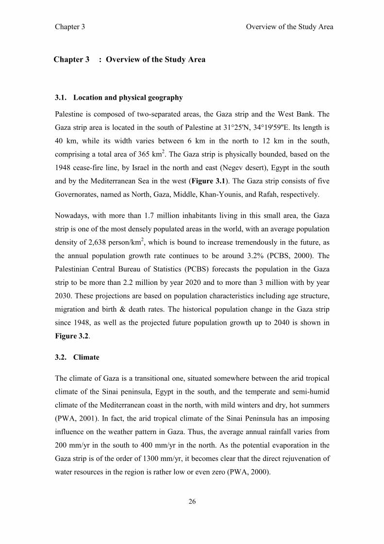
Chapter 3 Overview of the Study Area
26
Chapter 3 : Overview of the Study Area
3.1. Location and physical geography
Palestine is composed of two-separated areas, the Gaza strip and the West Bank. The
Gaza strip area is located in the south of Palestine at 31°25'N, 34°19'59''E. Its length is
40 km, while its width varies between 6 km in the north to 12 km in the south,
comprising a total area of 365 km2. The Gaza strip is physically bounded, based on the
1948 cease-fire line, by Israel in the north and east (Negev desert), Egypt in the south
and by the Mediterranean Sea in the west (Figure 3.1). The Gaza strip consists of five
Governorates, named as North, Gaza, Middle, Khan-Younis, and Rafah, respectively.
Nowadays, with more than 1.7 million inhabitants living in this small area, the Gaza
strip is one of the most densely populated areas in the world, with an average population
density of 2,638 person/km2, which is bound to increase tremendously in the future, as
the annual population growth rate continues to be around 3.2% (PCBS, 2000). The
Palestinian Central Bureau of Statistics (PCBS) forecasts the population in the Gaza
strip to be more than 2.2 million by year 2020 and to more than 3 million with by year
2030. These projections are based on population characteristics including age structure,
migration and birth & death rates. The historical population change in the Gaza strip
since 1948, as well as the projected future population growth up to 2040 is shown in
Figure 3.2.
3.2. Climate
The climate of Gaza is a transitional one, situated somewhere between the arid tropical
climate of the Sinai peninsula, Egypt in the south, and the temperate and semi-humid
climate of the Mediterranean coast in the north, with mild winters and dry, hot summers
(PWA, 2001). In fact, the arid tropical climate of the Sinai Peninsula has an imposing
influence on the weather pattern in Gaza. Thus, the average annual rainfall varies from
200 mm/yr in the south to 400 mm/yr in the north. As the potential evaporation in the
Gaza strip is of the order of 1300 mm/yr, it becomes clear that the direct rejuvenation of
water resources in the region is rather low or even zero (PWA, 2000).

Chapter 3
Figure
Figure 3.2: Population change in the Gaza CMWU, 2009).
0
500,000
1,000,000
1,500,000
2,000,000
2,500,000
3,000,000
3,500,000
4,000,000
4,500,000
19
48
19
67
19
80
Pop
ula
tion
Overview of the Study Area
27
Figure 3.1: Location map of the Gaza strip.
Population change in the Gaza strip between 1948-2040
19
80
19
92
19
96
19
97
20
07
20
08
20
09
20
10
20
15
20
20
20
25
Year
Overview of the Study Area
2040 (PCBS, 1998;
20
30
20
35
20
40

Chapter 3 Overview of the Study Area
28
The average daily temperatures in Gaza are around 25 C0 in the summer and 13 C0 in
the winter, with the average daily maximum temperature ranging between 29 C0 and 17
C0, and the minimum temperature between 21 C0 and 9 C0, for the summer and winter
seasons, respectively. The daily relative humidity fluctuates between 65% in daytime to
85% at nighttime in summer and between 60% and 80% in winter. The mean annual
solar radiation is 2200 J/cm2/day (MEnA, 2000). There are significant variations of the
wind speed during daytime, with an average maximum of about 3.9 m/s. On the other
hand, storms with maximum wind speeds of 18 m/s have been observed in winter.
3.2.1. Rainfall
Rainfall is the most important component of groundwater recharge in the area. As
surface runoff is almost negligible, recharge is generally estimated as a portion of the
effective rainfall. In the Gaza strip 12 manual rainfall stations exists, distributed as
shown in Figure 3.3. Data at these stations are collected daily by the Ministry of
Agriculture (MoA). Table 3.1 presents the locations of these rainfall stations together
with the sizes of their Thiessen-polygon-delineated influence areas.
Figure 3.4 shows the average, maximum and minimum annual rainfall rates of all Gaza
rain stations for the time period 1990-2010. From the figure one may notice, in
particular, that the regional rainfall has decreased tremendously after the rainy season in
1999, and started to increase after the rainy season in 2000, and that after this time the
regional rainfall has oscillated and decreased once again after the rainy season in 2004.
The average annual rainfall in the Gaza strip, based on a 20-year-long record, is 320
mm/y, which results in a total amount of rainfall of about 116 million m3 /year for the
whole area. However, whereas the average annual rainfall is only 220 mm/year in the
south, due to the dominant influence of the arid tropical climate on the weather patterns,
it increases to 410 mm in the north, as indicated by the two barplots of Figure 3.5.

Chapter 3 Overview of the Study Area
29
Figure 3.3: Locations of rain stations in the Gaza strip with Thiessen polygon areas (adapted from PWA, 2000).
Figure 3.4: Time series of average annual rainfall for all 12 rain stations in the Gaza strip between 1990 and 2010.
0
100
200
300
400
500
600
700
800
900
Rai
nfa
ll (
mm
/yr)
Season
Max
Avg.
Min.
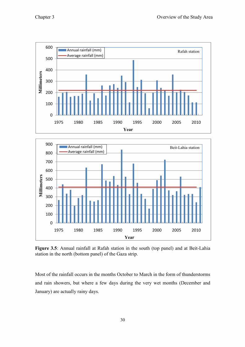
Chapter 3 Overview of the Study Area
30
Figure 3.5: Annual rainfall at Rafah station in the south (top panel) and at Beit-Lahia station in the north (bottom panel) of the Gaza strip.
Most of the rainfall occurs in the months October to March in the form of thunderstorms
and rain showers, but where a few days during the very wet months (December and
January) are actually rainy days.
0
100
200
300
400
500
600
1975 1980 1985 1990 1995 2000 2005 2010
Mi l
lim
eter
s
Year
Annual rainfall (mm)
Average rainfall (mm)Rafah station
0
100
200
300
400
500
600
700
800
900
1975 1980 1985 1990 1995 2000 2005 2010
Mi l
lim
eter
s
Year
Annual rainfall (mm)Average rainfall (mm)
Beit-Lahia station

Chapter 3 Overview of the Study Area
31
Table 3.1: Distribution Characteristics of rainfall stations in Gaza for year 2006-2007 (PWA, 2008).
Station no.
Station
name X_coord. Y_coord.
Average
rainfall (mm)
Total
rainfall (mm)
Thiessen area (km2)
1 Beit-
Hanoun 106420.00 105740.00 418 509.9 29.00
2 Beit-Lahia
99750.00 108280.00 433 530.3 14.25
3 Jabalia
99850.00 105100.00 421 536.7 15.50
4 Shati
97474.78 105428.23 392 469.0 2.250
5 Gaza-City
97140.00 103300.00 370 501.2 13.00
6 Tuffah
100500.00 101700.00 425 545.5 23.25
7 Gaza-South
95380.00 98000.00 394 388.2 35.00
8 Nusseirat
91950.00 94080.00 354 403.0 29.50
9 D-Balah
88550.00 91600.00 324 418.0 38.50
10 Khanyunis
84240.00 83880.00 290 252.0 83.50
11 Khuzaa
83700.00 76350.00 245 256.1 42.50
12 Rafah
79060.00 75940.00 236 225.0 38.75
Total
359 5035 365 km2
3.2.2. Evaporation
Evaporation measurements, based on a 25-year-long record, indicate that the long-term
potential evaporation in the Gaza strip is of the order of 1300 mm/yr, with the highest
evaporation rate of 138 mm occurring in months July and August, which are also the
hottest months of the year in Gaza. Meanwhile, the lowest evaporation rate, with only
63 mm, is measured in January. Further details of the monthly average evaporation and
rainfall values for Gaza city are shown in Figure 3.6 and Table 3.2.

Chapter 3 Overview of the Study Area
32
Figure 3.6: Average monthly rainfall and evaporation in Gaza city between 1980-2005.
Table 3.2: Average monthly climate variables for Gaza city (Israel Meteorological Service and PWA, 2000).
Month Average temperature
(C0)
Average evaporation
(mm)
Average rainfall
(mm)
January 13.6 63.4 83.3
February 14.0 73.1 55.3
March 15.8 94.1 41.2
April 18.0 116.4 8.9
May 21.3 133.4 3.7
June 23.8 135.5 0.0
July 25.7 137.8 0.0
August 26.2 137.8 0.0
September 25.2 124.9 0.7
October 22.9 113.7 15.6
November 19.8 91.0 70.9
December 15.4 78.7 91.8
63.4
73.1
94.1
116.4
133.4 135.5
137.8 137.8
124.9
113.7
91
78.7
83.3
55.341.2
8.9 3.7 0 0 0 0.7 15.6
70.9
91.8
0
20
40
60
80
100
120
140
160(m
m)
Month
Gaza average evaporationGaza average rainfall

Chapter 3 Overview of the Study Area
33
3.3. Topography
The elevation of the ground surface in the Gaza strip varies from 110 m AMSL (above
mean sea level) in the southeast and decreases in an irregular manner in northwest
direction to become 0 m at the coastline (Figure 3.7).
The topography of the coastal plain aquifer is characterized by elongated calcareous
sandstone (locally termed as Kurkar) ridges and sand dunes. These ridges extend more
or less parallel to the coastline and increase in height away from the shore in eastward
direction, up to a distance of a few kilometers offshore (Aish, 2004).
More specifically, there are four ridges: the coastal ridge (20 m MSL), the Gaza ridge
(up to 50 m MSL), the El Muntar ridge (80 m MSL), and the Beit Hanoun ridge (90 m
MSL). These ridges are separated by deep depressions (20-40 m MSL) which are filled
with alluvial deposits (see Figure 3.8).
3.4 Soil
The soil in the Gaza strip is composed mainly of six types: loess soil, dark
brown/reddish brown, sandy loess soil, loessial sandy soil, sandy loess soil over loess
and sandy regosol (PEPA, 1996), (see Figure 3.9). The sandy soil, whose chemical
composition is mainly quartz and alumina silicate, primarily, feldspar (Al-Agha, 1995),
is found in the form of sand dunes all along the coastline. Its thickness varies from 2 m
to about 50 m, following the hilly shape of the dunes. The sand dunes extend up to 4 to
5 km inland in the north and south, and to less in the center of the Gaza. Some of these
dunes are active, especially in the south between Deir El Balah and Rafah. The more
inland-located dunes, west of Khan Younis, are older dunes stabilized by vegetation.
Further inland to the east, the soil becomes less sandy and has more silt, clay, and loess.
Dark brown (clay) soil can be found in the northeastern part of the Gaza strip, whereas
the loess soil is located around Wadis, where it reaches a thickness of up to 25 to 30 m.
Table 3.3 summarizes the classification and characteristics of the different soil types
found in the Gaza strip.

Chapter 3 Overview of the Study Area
34
Figure 3.7: Topography of the Gaza strip (MOPIC, 1996).
Figure 3.8: 3-D topographical map view of the stratigraphy of the Gaza strip (adapted from Metcalf & Eddy, 2000).

Chapter 3 Overview of the Study Area
35
Table 3.3: Classification and characteristics of the different soil types in Gaza strip (adopted from MOPIC, 1997; Goris and Samain, 2001).
Texture Description Location Local
classification
Sandy loam (6%
clay, silt 34% , sand
58%)
Loess soils sedimented in Pleistocene
until Holocene Series. The grain size of
loess fluctuates from 0.002 to 0.068 mm.
Loess has been transported by winds and
sedimented in loose form in the upper
part, and in hard form in the lower part
of the layers. They are brownish yellow-
colored often with accumulation of lime
concretions in the subsoil and containing
8 – 12 % calcium carbonate.
Between the
Gaza city and
the Wadi Gaza
Loess soil
Sandy clay loam
(25% clay, 13%
silt, 62% sand)
These alluvial soils are usually dark
brown to reddish in colour, with a well-
developed structure. At some depth,
lime concretions can be found. The
calcium carbonate content can be around
15–20%
Beit Hanoun and
Wadi Gaza
Dark brown
/reddish brown
Sandy clay loam
(23% clay, 21%
silt, 56% sand)
This is a transitional soil, characterized
by a rather uniform, lighter texture.
Apparently, windblown sands have been
mixed with loessial deposits.
Deir-Balah and
Abasan
Sandy loess
soil
The top layer is
sandy loam (14%
clay, 20% silt, 66%
sand). The lower
profile is loam
(21% clay, 30%
silt, 49% sand)
Forms a transitional zone between the
sandy soil and the loess soil, usually
with a calcareous loamy sandy texture
and a deep uniform pale brown soil
profile.
It is found in the
central and
southern part of
the strip
Loessial sandy
soil
Sandy loam (17.5%
clay, 16.5% silt,
66% sand)
It is loess or loessial soils which have
been covered by a 20 to 50 cm thick
layer of sand dune
It is found east
of Rafah and
Khan Younis
Sandy loess
soil over loess
Top layer is loamy
sand (9% clay, 4%
silt, 87% sand).
Deeper profile is
sand (7.5% clay,
0% silt, 92.5%
sand)
Soil without a marked profile. Texture in
the top meters is usually uniform and
consists of medium to coarse quartz sand
with a very low water holding capacity.
The soils are moderately calcareous,
very low matter and chemically poor,
but physically suitable for intensive
horticulture in greenhouses. In the
deeper subsurface occasionally loam or
clay loam layers of alluvial found.
It is found a long
the coast of
Gaza strip
Sandy regosol
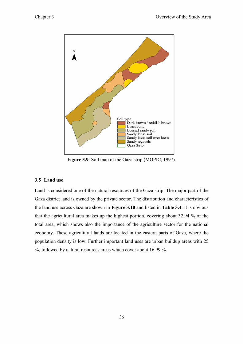
Chapter 3 Overview of the Study Area
36
Figure 3.9: Soil map of the Gaza strip (MOPIC, 1997).
3.5 Land use
Land is considered one of the natural resources of the Gaza strip. The major part of the
Gaza district land is owned by the private sector. The distribution and characteristics of
the land use across Gaza are shown in Figure 3.10 and listed in Table 3.4. It is obvious
that the agricultural area makes up the highest portion, covering about 32.94 % of the
total area, which shows also the importance of the agriculture sector for the national
economy. These agricultural lands are located in the eastern parts of Gaza, where the
population density is low. Further important land uses are urban buildup areas with 25
%, followed by natural resources areas which cover about 16.99 %.

Chapter 3 Overview of the Study Area
37
Figure 3.10: Land use map of Gaza strip (Shomar et al., 2010).

Chapter 3 Overview of the Study Area
38
Table 3.4: Characteristics and distribution of land use in Gaza (adapted from Shomar et al., 2010).
ID Land use type Area (Km2) Percent (%)
1 Airport 7.5 2.05
2 Built-up 91.25 25.0
3 Cultivated 120.23 32.94
4 Existing industrial area 0.9 0.25
5 Wastewater treatment site 0.45 0.12
6 Fisheries site 0.3 0.08
7 Harbor 0.35 0.1
8 Important natural resource 24 6.58
9 Mawasi 14.5 3.97
10 Natural resources 62 16.99
11 Natural reserve 26.5 7.26
12 Proposed treatment site 1.1 0.3
13 Recreation 6.1 1.67
14 Roads 9.8 2.68
Total Area 365 100
3.6. Geology
The geology of the aquifer system, that extends along the coastal plain of the Gaza strip,
is of the Pliocene- Pleistocene age, consisting mainly of marine deposits of sandstone,
calcareous siltstone and red loamy soils. Moreover, a series of geological formations
sloping gradually westwards is found, which are mainly from the Tertiary and
Quaternary ages. The geological components in the area consist of a littoral zone, a strip
of dunes from the Quaternary era, situated on the top of a system of older Pleistocene
beach ridges and, more to the east, gently sloping alluvial and loessial plains
(EPD/IWACO-EUROCONSULT, 1994). Most of the Gaza strip is covered by
Quaternary soil, whose clayey material content is increasing towards the east. Table 3.5

Chapter 3 Overview of the Study Area
39
summarizes the geological history of the area, as obtained from oil exploitation logs
going down to depth of up to 2000 m.
Table 3.5: Geology and history of the Gaza aquifer (PEPA, 1994).
Era
Epoch Age 106
(year BP)
Formation depositional environment
Lithology Thickness
(m)
Water
bearing
character
Quaternary
Ho
loce
ne
0.01
Alluvial
Terrestrial
Sand, loess,
calcareous silt and gravel
25 Locally phreatic aquifer
Ple
isto
cen
e
1.8 Continental Kurkar
complex
Eolian fluvial
Calcareous
sandstone
and
loamy sand
100 Main aquifer
Marine Kurkar
Near shore Calcareous
sandstone,
limestone
(sandy
and
porous)
100 Main aquifer
Tertiary
Pli
ocen
e
12 Conglomerates
Near shore
20 Base of the coastal zone aquifer
Saqiya Shallow marine
Clay, marl, shale
1000 Aquiclude
Mio
cene
25 Marine Marl,
limestone,
sandstone
and
chalk
500 Aquiclude alternating permeable layers with saline water

Chapter 3 Overview of the Study Area
40
3.6.1. Tertiary formation
The tertiary formation is mainly composed of the Saqiya formation deposits of the
Pliocene and Miocene ages, consisting of marine clay, shale and marl. The Pliocene
epoch formation has a thickness of about 1000 m at the shoreline and decreases rapidly
towards the east. Well-log information from oil exploitation activities going down to
depths of over 2000 m indicate further that the underlain Miocene formation consists of
chalks, limestone, and sandstone. With regard to hydrogeology (see next section), the
low permeability of the tertiary formation defines the latter as a lower, bottom aquiclude,
which is considered further in the conceptual groundwater model, to be discussed later.
3.6.2. Quaternary formation
The Quaternary deposits in the area cover the Pliocene Saqiya, with a thickness of about
225 m. The overlying Pleistocene deposits consist of the following formation from
bottom to top:
1. Marine Kurkar formation
This formation is mainly of Pleistocene marine origin, and its constituents are medium to
coarse quartz sandstone and calcareous shell fragments, cemented by calcite (El-Nakhal,
1968; Al-Agha, 1995). The marine Kurkar has a high porosity and permeability, due to
the abundance of large voids. Within the Gaza strip, the total thickness of the Kurkar
group ranges between 100 m at the shore in the south and 10 m near at its east border
(PWA, 2001).
2. Continental Kurkar formation
This formation, also of Pleistocene origin, and of eolian fluvial nature, is referred to
locally as Continental Kurkar or Jarwal. It has a maximum thickness of 100 m (El-
Nakhal, 1968). The coastal 1- 4 km- wide belt along the Mediterranean Sea is covered
with calcareous sand dunes, which are important for the natural recharge of the coastal
aquifer.
3. Recent deposits These deposits are found at the top of the Pleistocene formation and have a thickness of
up to 25 m. They can be divided into four different types:

Chapter 3 Overview of the Study Area
41
a. Sand dunes:
These dunes extend along the shoreline, especially near Rafah and Beit-Lahia and
originate partly from Nile river sediments. The thickness of these dunes is about 15 m,
and their width is small in the south, but increases to up to 3 km in the north.
b. Sand, loess and gravel beds:
This formation has a thickness of only 10 m and it is the main formation of the Wadi
Gaza area (near surface), where the Wadi fillings consist of sand, loess and gravel beds.
c. Alluvial deposits:
These deposits are widely distributed across an area extending from the Wadi Gaza
northwards, and are dominated by heavy, loamy brown clay with a thickness of about 25m.
d. Beach formation:
The beach formation, locally termed as Zufzuf, is composed of a relatively thin layer of
sand with shell fragments and is mainly unconsolidated, although in some places it is
cemented, due to the precipitation of calcium carbonate.
3.7. Hydrogeology of the Gaza coastal aquifer
3.7.1. Hydrogeological stratification
The larger Gaza coastal aquifer covers an area of about 2000 km2 and extends along
some 120 km of the Mediterranean coastline from the Gaza strip in the south, where its
width is about 20 km, to Mount Carmel in the north, with a width of only 3-10 km
(Figure 3.11). Under natural conditions, the groundwater flow in the Gaza strip is
generally directed from east to west, towards the Mediterranean Sea (Mercado, 1968).
This means that a large portion of the recharge of the Gaza section of the aquifer occurs
on the territory of Israel in the east. This horizontally-directed subsurface flow into the
Gaza aquifer is known as lateral inflow and its amount from the upstream Israeli side
varies from year to year. As a matter of fact, it has been reported to have decreased over
recent years, to due increased groundwater abstraction along the Israeli side of the
border.

Chapter 3 Overview of the Study Area
42
Figure 3.11: Coastal aquifer with groundwater flow regime (adapted from PWA, 2003).
Metcalf and Eddy (2000) estimated the amount of inflow to be in the range of 15 and 30
Mm3/year, whereas Ba’lousha (2005) gave a value of 26 Mm3 for year 1990. Actually,
in this study the lateral flow was estimated at 21 Mm3 for year 2000 and projected to
reduce to 12 Mm3 for year 2010. This large decrease of the lateral inflow over a
timespan of only 20 years can only be seen as a sign of “stealing” of groundwater by
excessive pumping at the Israeli side of the eastern Gaza strip border.
Fig. 3.12 shows the hydrogeological EW- cross sectional scheme of the Gaza aquifer
system. Near the coast in the west this aquifer is subdivided into 4 separate sub-
aquifers: A, B1, B2, and C, which together form a largely unconfined and
confined/unconfined multi-aquifer system (PEPA, 1996). Marine clay layers with a

Chapter 3 Overview of the Study Area
43
Figure 3.12: Schematization of hydrogeological EW-cross section of the Gaza coastal aquifer (PWA, 2003).
Figure 3.13: Schematic general hydrogeological SE-NW cross section of the coastal aquifer in the northern Gaza area (Vengosh et al., 2005).
thickness of 20 meters that act as aquicludes and which are sloping slightly towards the
sea separate these sub-aquifers within a distance of about 2-5 km inland from the
shoreline. These clay layers then pinch out further in the east, so that over most of the

Chapter 3 Overview of the Study Area
44
rest of aquifer cross section in the east only a single phreatic (unconfined) aquifer with a
thickness of 80-100 m is defined.
Referring to Figure 3.12, the aquifer system can be described more specifically as follows:
Upper sub-aquifer A
The uppermost aquifer which is classified as sub-aquifer A and extends from the
shoreline to the east up to 2 km. This aquifer is bounded from the top by the water table
and at the bottom partly by the first aquitard of silty clay. The thickness of this aquifer
varies between 10 to 30 meters.
Middle sub-aquifers B1 and B2
These two sub-aquifers, classified as B1 and B2, consist mainly from Kurkar and micro-
conglomerate. They are considered as partly confined/unconfined aquifers, as the
separating semi-permeable clay layer, which is made up of clay with chalk and silty
sand, extend about 5 km to the east. The thicknesses of these sub-aquifers range between
40 and 50 m.
Lower sub-aquifer C
The lower sub-aquifer, classified as C, is again a confined/unconfined aquifer, with an
EW-extension of about 5 km. Its main constituents are sand and chalk with some
conglomerate in the middle. The sub-aquifer is partly bounded by the second semi-
permeable layer at the top and by the clay Saqiya group formation at the bottom, which
forms also the base of the aquifer. The latter goes down to a depth of 1900 m near the
coastline, but wedges out gradually in eastward direction.
Although the EW- cross section of the hydrogeological stratification of the Gaza
aquifer shown in Figure 3.13 is very representative for the aquifer system as a whole
and Gaza aquifer as a part, there are differences across the study region. Thus the
maximum thickness of the coastal aquifer is in the northwest, close to the coast, and
decreases gradually towards the east and southeast.

Chapter 3 Overview of the Study Area
45
In the Gaza strip itself, the main characteristics of the aquifer as well as its structure
and thickness vary significantly from north to south as follows:
In general, the average thickness of the Gaza aquifer is about 150 m, but it is only
80-100 m in the north of the eastern boundary (near the Gaza-Israel border). Moreover,
the thickness decreases to only a few meters at the eastern aquifer boundary and beyond
on the Israel territory (see Figure 3.13).
In the southeast section of the eastern border of the Gaza strip the aquifer thickness
decrease to less than 10 m.
The structure and the thickness of the aquifer vary significantly from north to south in
the Gaza strip. Thus, whereas in its northern section, the aquifer thicknesses in the western
and central areas are 180-200 m, they decrease to 140 - 160 m in the central Gaza strip, and
reach only 100 - 120 m and in its southern part.
Although along the north-south transect no change in the basic structure of the sub-
aquifer division along the coast is observed, the thickness of the lower sub-aquifer C
decreases significantly (Vengosh et al., 2005).
The depth from the ground surface to the water table ranges from about 8 m in the west
near the shore, to 90 m in the east of the Gaza district.
3.7.2. Hydraulic aquifer properties
Important hydraulic aquifer parameters have been obtained from pumping tests, which
were carried out in different municipal wells, as a part of the project of CAMP-2000 and
under the monitoring of the Palestinian Water Authority (PWA). The results of these
aquifer tests indicate that the transmissivity values T range between 700 and 5,000
m2/day, whereas the corresponding values of the hydraulic conductivity K were
estimated to lie in a relatively narrow range of K = 20-80 m/day, i.e. K = 2.31 x10⁻⁴ –
9.26 x10⁻⁴ m/s (PWA/USAID, 2000b).
Values for the specific yield Sy for the unconfined aquifer were found to be in the range
of 0.15–0.30, while the specific storage Ss for the confined units turns out to be about
10−4 m-1. Table 3.6 summarizes these initial aquifer hydraulic parameters.

Chapter 3 Overview of the Study Area
46
Table 3.6: Range of hydraulic parameters obtained from aquifer tests (PWA/USAID, 2000b).
Parameter Value
Transmissivity (m2/d) 700 - 5000
Hydraulic conductivity (m/d) 20 - 80
Specific yield 0.15 – 0.30
Storativity (m-1) 10-4 - 10-5
3.8. Water resources
Groundwater is the main natural resource in the Gaza strip. In fact, the Mediterranean
coastal aquifer of the Gaza strip is the only source of water supply. Although there is a
limited water resource available from the surface water system in the Gaza strip,
namely, the wadis, the latter are completely dry for most of the time. This is why it is
assumed in this study that groundwater is the only available resource in the Gaza area.
3.8.1. Surface water
The surface water system in the Gaza strip consists of valleys, which are locally named
wadis. These wadis are completely dry in summer and flood occasionally for short
periods during winter. The major wadi is Wadi Gaza which originates in the Negev
Desert and crosses the Gaza strip in its central part. Its length is about 105 km, out of
which only 9 km are located within the Gaza district, and its catchment area is 3500 km2
(Figure 3.14). Wadi Gaza has two main sources: Wadi Al Sharia, which collects water
from the Hebron Mountains in the west Bank and Wadi Al Shallala, which collects
water from the height of the northern Negev desert.
In 1994 the average annual runoff was estimated at 40 Mm3, unfortunately, nowadays
this rate has gone down to 2 Mm3. This large reduction in runoff entering the Gaza strip
is due to the Israeli practices of diverting large amounts of Wadi water into a dam for
storage projects in Israel, just before it reaches Gaza. Another problem is the pollution

Chapter 3 Overview of the Study Area
47
Figure 3.14: Wadi Gaza catchment area and boundaries (Aliewi, 2009).
of the Wadi Gaza by sewage collected from towns and camps in the central areas of the
Gaza strip.
Other small and insignificant wadis in the Gaza strip are Wadi El-Salqa near Deir El-
Balah town, with a catchment area of 20 km2, and Wadi Beit-Hanon in the north which
crosses the northeastern border of the Gaza strip and flows out again across the northern
border to Israel. Its catchment area is similar in size to that of Wadi El-Salqa. Actually,
the flows from these two wadis are not stored or used. In fact, surface water resources
are presently not used at all in the Gaza district (MEnA, 2000).

Chapter 3 Overview of the Study Area
48
3.8.2. Groundwater
Groundwater is practically the only fresh water source available in the Gaza strip. The
annually sustainable yield of the coastal aquifer underlying Gaza is dependent upon the
climatic conditions. At present, the Gaza coastal aquifer is a dynamic system with
continuously changing inputs and outputs. High rates of urbanization and increased
municipal water demand, as well as extended agricultural activities, have led to an
overexploitation of this aquifer over recent decades. This has nowadays created a
negative balance, where more water is pumped out the aquifer than is replenished by
natural recharge. In consequence, this has led to a decline in the net storage and to large
drop of the ground water levels in recent times, as will be discussed in details, in the
following paragraphs.
To come up with a first estimate of the water balance for the Gaza coastal aquifer, the
following fundamental equation is used:
Balance = Sum (inflows) – Sum (outflows) (3.1)
where inflows and outflows comprise all water inputs and outputs to the aquifer body,
respectively. These are shown in Figure 3.15. Thus the inflow components consist of
the effective recharge as direct infiltration of rainfall, lateral inflow from the Israeli side,
total return flow from irrigation and leaked water, as well as saline seawater from the
sea, the latter being a result of seawater intrusion. Outflows represent all external
stresses on the aquifer, and consist mainly of agricultural and municipal abstractions, in
addition to a small amount of groundwater discharge to the sea (Figure 3.15).
Table 3.7 shows the existing and projected inflow and outflow components for the Gaza
aquifer system within the period 2000-2020, under the conditions that there are no new
water resources available to recover the sustainability of the Gaza aquifer and Figure
3.16 illustrates the overall aquifer balance for the current situation and the future
projections. One may notices from this figure that there has been a water balance deficit
of about 68.35 Mm3 in year 2010, which is expected to reach more than 89.5 Mm3 by
year 2020.

Chapter 3
Figure 3.15: 3-D representation of(adapted from Metcalf and Eddy, 2000).
Figure 3.16: Estimated Gaza aquifer balance deficit for 2000
-100
-90
-80
-70
-60
-50
-40
-30
-20
-10
0
2000
Def
icit
(M
CM
)
Overview of the Study Area
49
D representation of water-balance components for the Gaza aquifer(adapted from Metcalf and Eddy, 2000).
Estimated Gaza aquifer balance deficit for 2000-2020 time period.
2005 2010 2015
Year
Deficit
Overview of the Study Area
balance components for the Gaza aquifer
2020 time period.
2020

Chapter 3 Overview of the Study Area
50
Table 3.7: Estimated water balance of the Gaza strip for time period 2000-2020 (adapted from Metcalf & Eddy, 2000).
Year 2000 2005 2010 2015 2020
INFLOW
Rainfall and lateral Recharge (Mm3)
65.0 64.0 62.1 62.1 61.2
Irrigation return (Mm3)
22.75 22.5 21.25 20 20
Domestic return flow (Mm3)
11.2 15 18.8 21.41 24.8
Wastewater return flow
8.5 8.5 8.5 8.5 8.5
Total (Mm3)
107.45 110 110.65 112 114
OUTFLOW
Municipal abstraction (Mm3)
56 75 94
107 124
Agricultural abstraction (Mm3)
91.0 90 85 80 80
Total (Mm3)
147 165 179 187 204
Deficit -39.55 -55 -68.35 -75 -89.5
3.9. Wells
The agriculture sector is the backbone of the Palestinian economy and represents about
64% of the total water consumption. More than 4000 water wells have been dug across
the Gaza strip and can be classified as agricultural or domestic wells (Figure 3.17). In
fact, the majority, with about 3850 wells, are used for agriculture purposes and
distributed along the Gaza strip (Figure 3.18). Approximately 137 wells are owned and
operated by individual municipalities and used for domestic supply, 13 wells owned by
UNRWA. The average density of wells is about 5 per km2, although in some areas in
the north of Gaza, the density of wells exceeds 20 per km2.
Most of agricultural wells in Gaza are shallow and penetrated only 5-15 m below the
groundwater table, tapping almost exclusively the sub-aquifer “A”, whilst the municipal
wells are deeper and may tap sub-aquifers “A” and “B”,depending on location and
distance from the coast (PWA, 2001a) (see Figure 3.12).

Chapter 3 Overview of the Study Area
51
Figure 3.17: Map of 4000 municipal and agricultural water wells across the Gaza strip.
Figure 3.18: Distribution of 3850 agriculture water wells across the Gaza strip.
80000 85000 90000 95000 100000 105000
75000
80000
85000
90000
95000
100000
105000
110000
A-180
A-185C-127
C-128
C-76
C-79AD-2
D-601
D-67
D-68
D-69
D-70
D-71
D-72
D-73
D-74
Debri
E-1
E-142
E-154
E-156E-157
E-4
E-6 E-61
E-90
G-16
G-30
G-49
J-146
J-32
K-19
K-20K-21
L-127
L-159L-159A
L-176
L-179A
L-182
L-184
L-187
L-189
L-41
L-43
L-87
L-I286
Mog
Mog1
Msalam
Mun.
New
P-124
P-138
P-139
P-144
P-15
P-153
P-52
priv.
Q-40A
Q-68
R-112R-113
R-162BA
R-162CA
R-162D
R-162EA
R-162G
R-162HR-162HA
R-162LR-162LB
R-254
R-25AR-25BR-25CR-25D
R-265
R-74
R-75
S-37
S-69
S-72
N1
N10
N11
N14
N15
N16
N17N18
N19
N2
N20N21
N22
N23
N24N25
N3
N4 N5
N6
N7
N8
N9
Y1Y2
Y3
Y4
Y5
T26
T27
T28
T30
T31T32
T33T34
T35
T38
T39
T4
T40
T41
T6
T8
T9
kh137
T12
T13
T14T15
T16T17
T18 T19
T2
T20T21
T22T23
T24
T25
M1
M10
M2A
M2B
M3
M4 M5
M6
M7
M8
M9
MI1
MI2
MI3
L11
L110L111
L112L113
L114
L115
L116L117
L118
L119
L120L121
L122L123
L124
L126
L128
L129
L13
L130
L131
L132
L133
L134L135
L136
L137L138
L139
L14
L140
L141
L142
L143
L144
L145
L15
L150
L151L153
L154L155
L156
L157
L16
L160
L161
L162
L163
L164
L165
L166
L167
L17
L170
L172
L173
L174
L177
L178
L179B
L18
L19L20L21L22
L24L25
L26L27
L28 L29
L30
L31 L32
L33
L34
L35
L36
L37
L38
L39
L4
L40
L42
L45
L46
L47L48L49
L5
L66
L67
L68L69
L7
L70
L71L72 kh1
kh5
kh6
kh31
kh32
kh44
kh49
kh53
kh54
kh55
kh63
kh74
kh80
kh90
kh114
kh116kh127
kh128
kh145
kh163
kh172
kh184
kh191
kh233
kh234
kh245
kh286
Raf11
Raf14
Raf25Raf39
Raf46
Raf51
Raf64
Raf77
Raf80
P51
P53
P54
P55
P56P57
P58
P59
P6
P60
P61
P62
P63
P64P65
P66
P67P69
P70
P71
P72
P73P74
P75
P76P77
P78
P79
P80
P81
P82
P83
P84P85
P86AP86B
P86C
P88
P89P90
P91
P92
P93P94
P96
P97
P98P99
P120
P121P122
P123
P125
P126
P127
P13
P130
P131
P132
P133
P135
P136
P137
P140
P141
P142
P145
P147
A1
A10
A100
A101A102
A103
A104
A104A
A105
A106
A107
A108A109
A11
A110
A111
A113A114
A115
A116
A117
A118
A119
A12
A120
A121
A122
A123
A124
A125
A126
A127 A128A129
A13
A130
A131A132
A133
A134
A136
A137
A138
A139
A14
A140
A141A142
A143
A144
A145
A146
A147
A148A149
A15
A150
A151
A152
A153
A154
A156
A157
A158
A159
A16
A160
A161
A162
A163
A165
A166
A167
A168
A169
A17
A170
A171
A172
A173
A174
A175
A176
A177
A178
A179
A18
A181
A182
A183
A184A186
A187
A188
A189
A19
A190
A191
A192
A193
A194
A20A21
A22A23
A24A25A26A27 A28
A29
A2A
A2B
A2C
A2D
A3
A30
A31
A32A33
A34
A35
A37
A38
A39
A4
A40
A41
A42
A43
A44
A45
A46
A47A48
A49
A5
A50A51
A52A53
A54
A55 A56A57
A58
A59
A6
A60
A61
A62A63
A64
A65
A66
A67A68A681
A69
A7
A70
A71
A72A73
A74
A75
A76
A77
A78
A79
A8
A80
A81A82
A83
A84
A86A87
A88A89
A9
A90A91
A92A94A95A96
A97A98
A99
C1
C10
C100C101
C102
C103C104
C105
C106
C107C108C109
C110C111
C112
C113
C114
C115
C116
C117
C118
C119 C11A
C11B
C120
C121 C122
C123
C124
C125
C126
C129
C12A
C12BC12C
C12D
C13
C130
C14
C15A
C15B
C16A
C16B
C17A C17BC17CC18
C2
C20
C21C22
C23C24 C25
C26
C27
C28
C29
C30
C31C32C33
C34
C35
C36
C37
C38C39
C3A C3B
C3C
C3D C3E
C40
C42
C43
C44C45
C46
C47A
C47B
C48
C49
C4A
C4B
C5
C50
C51
C52C53
C54
C55AC55BC56AC56B
C57
C58C59
C6
C60
C62
C63
C64C65
C66
C67
C68
C69
C7
C70
C71
C72
C73C74
C75
C77
C78
C79
C8
C80C81C82C83
C84
C85C86
C87
C88C89
C9
C90C91 C92
C93C94
C95
C96
C97
C98C99
C-I-1
C-I-10
C-I-11
C-I-12
C-I-13C-I-14
C-I-15
C-I-16
C-I-17
C-I-2
C-I-3
C-I-4
C-I-6
C-I-7C-I-8
C-I-9
Q1
Q2
Q23Q24Q25
Q26Q27
Q28
Q29
Q14Q15
Q16
Q17Q18
Q20Q21
Q22
Q19 Q10
Q11
Q12
Q13
B1
B10
B11B12B13
B14B15
B16B17
B18
B19
B2
B20
B21
B22
B23
B24
B25
B3B4
B5
B6
B7 B8B9
D16D17
D18
D20D21D22
D23
D24D25
D26
D27
D28
D29
D3
D30D31
D32
D33D34 D35D36
D37D38
D39
D4
D40
D41 D42D43D44D45
D46
D47D48D49
D5
D50D51
D52D53
D54D55
D56
D57
D58
D59
D6
D61
D62
D63
D64
D65
D66
D7
D8
D9
E110E111E112
E113E114A
E115E116
E117E118
E119
E11A
E11BE11C
E12
E120
E121
E122
E123
E124
E126
E128E129
E13
E130
E131
E132
E133
E134
E135
E136
E137
E138
E14
E143
E144
E145E146
E147E148
E149
E15
E150
E152
E153
E155E158E159
E16
E160
E17
E18E19
E21
E22
E23E24AE24B
E25
E26
E28
E3
E30E31
E32
E33E33A
E34
E35
E36E37
E38E39
E40E41 E42
E43
E44
E45
E46 E48
E49 E5E50
E51E52
E53E54
E55 E56E57
E58E59
E6
E60
E62
E63 E64E65E66
E67E68
E68A
E69
E7
E70E71
E73 E74
E75E76E77
E78E79E80
E81E82
E84
E85E86
E87E88E89
E91
E93E94
E95E96E97
E98E99
F121F122
F122'
F123F124F125
F126F127
F128
F129
F13
F130A
F130B
F131F132F133
F134F135
F136
F137
F137n
F138F139
F14
F140
F141
F142
F143
F144
F145
F146
F147
F148
F149
F15
F150
F151
F152
F153F154F155
F156 F157
F158
F159
F16
F160
F161
F162
F163
F164
F165
F166
F167
F168F169
F17
F170
F171
F172
F173
F174
F176F177
F178F179
F18
F180
F181
F182
F183
F184
F185
F186
F188
F189
F19
F191
F2
F20F21
F23A
F23B
F24F25F26
F28
F29
F30A
F30B
F31F32
F33
F34
F35
F36
F38
F39
F4
F40
F41F42
F43
F44
F45
F46
F47
F48F49
F5
F50F51
F52F53
F54F55
F56
F57F58
F59F60
F61
F62F63F64
F65
F66
F67
F68AF68B
F69A
F69B
F7
F70
F71 F72
F73F73A
F74
F76
F76A
F77F78 F79
F8
F80F81F82F83F84
F85
F86F87
F89
F9
F90
F91
F92
F93F94F95 F96
F97
F98F99
G27
G28
G3
G31
G32
G33
G34
G35
G36G37
G38G39
G40
G41
G42
G43
G44
G45
G4AG4B
G5
G50
G501
G502
G503
G504
G505AG505B
G507
G508
G509
G510
G511
G512
G513
G6
G7G8G9
Gaz1
Gaz100
Gaz101
Gaz102Gaz103
Gaz104
Gaz105
Gaz106
Gaz107
Gaz108
Gaz109
Gaz11
Gaz110
Gaz111
Gaz113
Gaz114
Gaz115
Gaz116
Gaz117
Gaz118
Gaz119
Gaz12
Gaz120
Gaz121
Gaz122
Gaz123
Gaz124
Gaz125
Gaz126
Gaz127
Gaz13
Gaz14
Gaz15
Gaz16
Gaz17
Gaz18
Gaz2
Gaz20
Gaz21
Gaz22
Gaz23
Gaz24
Gaz25
Gaz27
Gaz28
Gaz29
Gaz3
Gaz30
Gaz31Gaz32
Gaz33
Gaz34Gaz35
Gaz36
Gaz37
Gaz38
Gaz39Gaz4
Gaz40
Gaz41
Gaz42
Gaz43
Gaz44
Gaz45
Gaz46
Gaz47
Gaz48
Gaz49
Gaz5
Gaz50
Gaz51
Gaz52
Gaz53
Gaz54
Gaz55
Gaz56
Gaz57
Gaz58
Gaz59
Gaz6
Gaz60
Gaz61
Gaz63
Gaz64
Gaz65
Gaz66
Gaz67
Gaz68
Gaz69
Gaz7
Gaz70
Gaz71
Gaz72
Gaz74
Gaz75
Gaz76
Gaz77
Gaz78
Gaz8
Gaz80
Gaz81
Gaz82
Gaz83
Gaz84
Gaz85
Gaz86
Gaz87
Gaz88
Gaz89
Gaz90
Gaz91
Gaz92
Gaz93
Gaz94
Gaz95
Gaz96
Gaz97
Gaz98
Gaz99
H10
H1001
H1002H1003
H1005H1006H1007
H1008
H1010
H11H12
H13H14
H15H16H18
H19
H2
H20
H21
H23
H24
H25
H26
H27H28
H29
H3
H30
H32
H33
H34 H35
H36H37H38
H39
H4
H40
H41
H42
H43
H44H45
H47
H49
H5
H50
H501 H502H503
H504
H505H506
H507
H508H509
H51
H510
H511 H512
H513
H514H515
H516
H517
H518H519
H52
H520H521
H522
H524
H525
H527
H528
H529A H53
H531H532
H533
H534
H535
H537
H538
H539
H54
H540H543
H57
H58H59
H6'
H60
H61
H62H63
H64
H65
H67
H69
H7
H70
H72H73
H74
H77
H78
H8
H80
H81n
H82
H83
H84
H85
H86
H87
H88
H9
H90
H91
H92
H93
J1
J10
J100
J1001
J1002
J101
J102
J103J104 J106
J107
J108
J109
J11
J110
J111
J112
J114
J115
J116 J117J118
J119
J12
J120
J121
J122
J124
J125
J126'
J127
J128
J13
J130
J131
J133
J134
J135
J136
J137 J138
J139
J14
J141
J142
J143
J144
J145
J148
J149
J15
J151
J153
J154
J16
J17J18
J19
J2
J20
J21
J22J23
J24J25
J27
J28
J29
J3
J30J36
J37
J4
J43
J44
J45J46J47J48
J49J50
J501
J502J504
J507
J509
J51J52
J54A
J54B
J54CJ54DJ54E
J55J56J57
J58
J59
J6
J60
J61J62J63J64
J66
J67
J68
J7
J70J71
J72
J74 J75
J76
J77
J8
J80J83
J85
J86J87J88
J89
J90J91
J92J93
J94
J95J96
J97
J98
J99
K1
K10
K11
K12
K13
K14
K15K16
K17
K2K3
K4
K5
K6
K7
K8
K9
kh10
kh100
kh101kh102
kh103
kh104
kh105kh106
kh107
kh108
kh109
kh11
kh110kh111
kh112
kh113
kh115
kh117
kh118
kh119
kh12
kh120
kh121
kh122
kh123
kh124
kh125
kh126
kh129
kh131
kh132 kh133
kh134
kh136
kh138kh139
kh14
kh140
kh141
kh143
kh144
kh146
kh147
kh148
kh149
kh15
kh150
kh151kh152 kh153
kh154
kh155
kh156
kh157
kh158
kh159
kh16
kh160
kh161
kh162
kh164
kh165
kh166
kh167
kh168
kh169
kh17
kh170
kh171
kh173
kh174
kh175
kh176
kh177
kh178
kh179
kh18
kh180
kh181kh182
kh183
kh186
kh187
kh188
kh189
kh19
kh192
kh193
kh194kh195kh196
kh197
kh198
kh199
kh2
kh200
kh201
kh202
kh203
kh204
kh205
kh206
kh207
kh208 kh209
kh21
kh210
kh211
kh212
kh213
kh214kh215kh216
kh217
kh218
kh219
kh22
kh220
kh221
kh222
kh223
kh224
kh225
kh226
kh227
kh228
kh229
kh23
kh230kh231
kh232
kh235
kh236
kh237
kh238
kh239
kh24
kh240
kh242
kh243
kh244
kh247
kh248kh249
kh25
kh250
kh251
kh252
kh253kh254
kh255
kh256
kh257
kh258
kh259kh26
kh260
kh261
kh262
kh263
kh264
kh265
kh266
kh267
kh268
kh269
kh27
kh270
kh271
kh272
kh273
kh274
kh275
kh276
kh277
kh278
kh279
kh28
kh280
kh281
kh282
kh283
kh284
kh285
kh287
kh288
kh289
kh29
kh290
kh291
kh292
kh293
kh294
kh295
kh296kh297kh298
kh3
kh30
Kh300
Kh301
Kh302
Kh303
Kh305
Kh306
Kh307
Kh308
Kh309
kh310
kh311
kh312
kh313
kh314
kh315
kh316
kh317
kh318
kh33
kh34
kh35
kh36
kh37
kh38
kh39
kh4
kh40
kh41
kh42
kh43
kh45
kh46
kh47
kh48
kh50
kh51
kh52
kh56
kh57
kh58kh59
kh60
kh61
kh62
kh64
kh65
kh66
kh67
kh68
kh69
kh7
kh70
kh71kh72
kh76
kh77
kh79
kh8
kh81
kh82kh83
kh84
kh85
kh86
kh87
kh88
kh89
kh9kh91
kh92
kh93
kh94
kh95
kh96
kh97
kh98
kh99
KI1
KI2
KI3
L10
L1003
L1007
L1008
L101
L1011
L1012
L1014
L1015
l1016L1017
L1019
L102L103
L104
L105
L106
L107
L108
L109
L181
L1A
L1Bn
L1Bo
L2
L50
L501
L503
L504
L505L506L507
L508L509
L51
L510
L512L513
L514 L515L516
L517L519
L52L52'
L520L521
L522L523L524
L526
L527
L528
L529
L53
L532
L534
L536L537L539L540L541
L542L543
L545 L546
L547
L548
L55
L550L551L552L553L554
L555L556L557
L559
L56
L560
L562L563L564
L566
L569
L57
L570
L572L573L574L576
L577L578L579
L58
L580
L581L582
L583L587
L59
L591L592L593
L594
L595BL595A
L596L597L598
L6
L60
L602
L603
L605L607
L61
L612
L613
L615
L616L617
L618L619
L62
L621
L622
L624
L625nL625o
L626
L627
L628
L63
L630
L632
L635
L637L638'
L64
L641
L643L644
L647
L648
L65
L650
L73A
L73B
L73C
L74
L76
L77
L78
L8
L80
L81
L83
L84
L85
L86n
L88
L89
L9
L90
L91
L92
L93L94
L95 L96
Mid1
Mid10Mid100
Mid101
Mid103
Mid104 Mid105
Mid106
Mid107
Mid108
Mid109
Mid11
Mid110
Mid111
Mid112
Mid113
Mid114
Mid115
Mid116
Mid117Mid118
Mid119
Mid120
Mid121
Mid122
Mid123
Mid124
Mid125
Mid126
Mid127
Mid128
Mid129
Mid13
Mid130
Mid131
Mid132
Mid133
Mid134
Mid135
Mid136
Mid137
Mid138
Mid139
Mid14
Mid140
Mid141
Mid142
Mid143
Mid144
Mid145
Mid146
Mid147
Mid148
Mid149
Mid150
Mid151
Mid152
Mid153
Mid154
Mid155
Mid156
Mid157
Mid159
Mid16
Mid160
Mid161
Mid162
Mid164Mid165
Mid166
Mid167Mid168
Mid169
Mid17
Mid170
Mid171
Mid172
Mid173
Mid174
Mid175
Mid176
Mid177
Mid178
Mid179
Mid18
Mid19
Mid2
Mid20
Mid21
Mid22
Mid23
Mid24
Mid25
Mid26
Mid27
Mid29
Mid3
Mid30
Mid31
Mid32
Mid33
Mid34Mid35
Mid36
Mid37
Mid38
Mid4
Mid40Mid41
Mid42
Mid43
Mid44Mid45
Mid46
Mid47
Mid48
Mid49
Mid5
Mid50 Mid51
Mid52
Mid53
Mid54Mid55
Mid56
Mid57
Mid58
Mid59
Mid6
Mid60
Mid61
Mid62
Mid63
Mid64
Mid65
Mid66
Mid67
Mid68
Mid69
Mid7
Mid70
Mid71
Mid72
Mid73
Mid74
Mid75Mid76
Mid77
Mid78
Mid79
Mid8
Mid80
Mid81
Mid82
Mid83Mid84Mid85
Mid86
Mid87
Mid88
Mid89
Mid9
Mid90
Mid91
Mid92
Mid93
Mid94
Mid95
Mid96
Mid97
Mid98
Mid99
MSALM
NI5
Nor1
Nor10
Nor11
Nor12
Nor13
Nor14
Nor16
Nor17
Nor18
Nor19
Nor2
Nor20
Nor21
Nor22
Nor23
Nor24
Nor25
Nor26
Nor27
Nor28
Nor29
Nor3
Nor30
Nor31
Nor32
Nor33
Nor34Nor35
Nor36
Nor37
Nor38Nor39
Nor4
Nor40
Nor6
Nor7
Nor8
Nor9
P1008
P101
P1012P1015
P1017 P1018
P1019
P102
P1023
P1024
P1025
P1026
P103
P1032
P104
P105
P106P107
P108
P109P110P111
P112
P113
P114P116
P117
P118
P119
P12
P16B P17
P18
P2
P21
P22
P24
P26
P27
P28
P29
P31
P32
P33
P34
P35P36
P37
P38
P39P41
P42
P43P44
P45P46
P47
P48AP48B
P49
P50
P501
P506
Q3
Q30
Q31Q32
Q33Q34
Q35Q36
Q37
Q38Q39
Q4Q40B
Q41
Q42
Q43
Q44Q45
Q46Q47
Q48Q49
Q5
Q50
Q51
Q52
Q53Q54A
Q54B
Q54CQ54D
Q54E
Q54FQ55Q56
Q57
Q58
Q59
Q60
Q61
Q62Q63
Q64Q65
Q67
Q69
Q7
Q8
Q9
QI224AQI225A
R102
R103
R106
R107
R11
R110R111
R114
R116
R12
R120R121R123R124
R125R126
R127
R128R129
R13
R130
R132
R133
R134
R135
R136
R137
R138
R139
R14
R140R141
R142R143
R144
R146
R147
R15
R150R153
R155
R160
R161
R162A
R162B
R162C
R162ER162F
R162Hn
R162Ln
R16AR16B
R17
R170
R171
R174
R176R177
R178
R179
R18
R183
R184
R185
R186
R187R188
R189
R19
R190 R192
R193R194
R195
R197R198
R199
R2
R20R2011R202R203
R204R205
R206R207R208
R209
R210
R211
R212
R213
R214
R215
R216
R217 R218
R219
R22
R221R222
R223
R223n
R224
R225
R227R228
R23
R230
R231
R232
R233
R234
R235
R236R237
R238
R24
R241
R242
R243
R244
R245
R246
R247
R249
R250
R251
R252
R253
R255
R256
R257
R258
R259
R260
R261
R262
R263
R264
R26A R27R271
R272A
R273
R274
R275
R277
R28R29
R3
R30
R31
R32R33
R34R35
R36R37
R38
R4
R40R41R42
R43R44
R46
R47
R48
R49
R5
R50R51
R52
R53
R54
R56R57R58R59
R6
R60
R62R63
R65
R66AR66B
R67
R68
R69
R7
R72
R76
R79
R81
R82R83
R84
R85
R86R87
R88
R8A
R8B
R9
R90
R91R92
R93
R94
R96
R98R99
Raf1
Raf10
Raf12
Raf13
Raf15
Raf16
Raf17
Raf18
Raf19
Raf2
Raf20
Raf21
Raf22
Raf23
Raf24
Raf26
Raf27
Raf28
Raf29
Raf3
Raf30
Raf31
Raf33
Raf34
Raf35
Raf36
Raf37
Raf38
Raf4
Raf40
Raf41
Raf42
Raf43
Raf44
Raf45
Raf47
Raf48
Raf49
Raf5
Raf50
Raf52
Raf53
Raf54
Raf55
Raf56
Raf57
Raf58
Raf59
Raf6
Raf60
Raf61
Raf62
Raf63
Raf65
Raf66
Raf67
Raf68
Raf69 Raf7
Raf70
Raf71
Raf72
Raf73
Raf74
Raf75
Raf76
Raf78Raf79Raf8
Raf9
S52
S53
S54
S55
S56
S57
S58
S59
S6
S60
S61
S62
S63
S64
S65
S66
S68
S69
S7
S70
S71
S8
S9
24
27
29
25A
26B
D10
D11
D12
D13
D14D15
E10
E100E101E102
E103
E104E105
E106
E107
E108
E83
Nor5
Zimo
R1
R10
2A
36B
6A
8A
F100
F101F102
F103F104A F104B
F104C
F105F106
F107
F108
F109
F110
F111
F112F113
F114
F115
F116
F117
F118F119
F120
F120A
R101
Well3
Well4G24A
G24B
G24C
S1
S2
S4
S10
23
22A
3A
cost1
cost2
cost3
DIBRI
F1
G1
G10 G11
G12
G13
G14
G17
G18
G19
G2
G20G21
G22G23
G25
G26
G49
J54En
S45n
S12
S13S14
S15
S16
S17
S18S19
S21
S22
S23
S24
S25
S26
S27
S28
S29S30
S31S32
S33S34
S35
S36S38
S39S40
S41
S42
S44
S45
S46
S47
S48
S49
S50
S51
S72
F11F12
F10
T43
T1
T29T3
T36
T37A
T42
T44
T7
coast4
12
18
21
37B
coast5
EV02
K19
L96n
L127
L159L159A
L171
L176
L179A
L182
10A
7
13
P1027
P10
P100
P52
P1001
P1005
A-I-1
A-I-10
A-I-11
A-I-12
A-I-13
A-I-14
A-I-15
A-I-16
A-I-17
A-I-19
A-I-20
A-I-21
A-I-22
A-I-23
A-I-24A-I-25
A-I-26
A-I-27A-I-28
A-I-29
A-I-3
A-I-30
A-I-31
A-I-32
A-I-33
A-I-34
A-I-35
A-I-36A-I-37
A-I-38
A-I-39
A-I-4
A-I-40A-I-41
A-I-42
A-I-43
A-I-44
A-I-45
A-I-46 A-I-47
A-I-48
A-I-49
A-I-5
A-I-50
A-I-6A-I-7A-I-8A-I-9
B-I-1
B-I-2 B-I-3
E-I-10E-I-11
E-I-13
E-I-14E-I-15E-I-16
E-I-22
E-I-23
E-I-24E-I-25
E-I-6
E-I-8E-I-9
R-I-89
R-I-90
F-I-1
F-I-10
F-I-100
F-I-101
F-I-102
F-I-103F-I-104F-I-105
F-I-106F-I-107
F-I-109
F-I-11
F-I-110
F-I-111
F-I-112
F-I-113
F-I-114
F-I-115
F-I-116
F-I-118
F-I-119
F-I-12
F-I-120F-I-121
F-I-122
F-I-123
F-I-124
F-I-125
F-I-126
F-I-127
F-I-128
F-I-129
F-I-13
F-I-130
F-I-14
F-I-15
F-I-16
F-I-17
F-I-18
F-I-19
F-I-2
F-I-20
F-I-21
F-I-22F-I-23
F-I-25
F-I-26F-I-27F-I-28
F-I-29
F-I-3
F-I-30
F-I-31F-I-32
F-I-33F-I-34F-I-35
F-I-36
F-I-37
F-I-38
F-I-39
F-I-4
F-I-40
F-I-41
F-I-42
F-I-43
F-I-44
F-I-47
F-I-48F-I-49
F-I-5
F-I-50
F-I-51
F-I-52
F-I-53
F-I-54
F-I-55
F-I-56F-I-57
F-I-58F-I-59
F-I-6F-I-60F-I-61F-I-62
F-I-63
F-I-64F-I-65
F-I-66F-I-67
F-I-68F-I-69 F-I-7
F-I-70
F-I-71
F-I-73F-I-74
F-I-75
F-I-76F-I-78F-I-79
F-I-8F-I-80
F-I-81
F-I-82F-I-83
F-I-84
F-I-85
F-I-86F-I-87
F-I-88
F-I-89
F-I-9F-I-90
F-I-91F-I-92
F-I-93F-I-94
F-I-95
F-I-96F-I-97
F-I-98F-I-99
R-I-1
R-I-10
R-I-11R-I-12
R-I-13R-I-14
R-I-15
R-I-16R-I-17
R-I-18
R-I-19
R-I-2
R-I-20
R-I-21
R-I-22
R-I-23
R-I-24
R-I-25
R-I-26
R-I-27
R-I-28R-I-29
R-I-3
R-I-30
R-I-31
R-I-32
R-I-34R-I-35
R-I-36R-I-37
R-I-38R-I-39
R-I-4
R-I-40
R-I-41R-I-42
R-I-43
R-I-45
R-I-46
R-I-47
R-I-48
R-I-5
R-I-50
R-I-51
R-I-52
R-I-53
R-I-54
R-I-55
R-I-56
R-I-57
R-I-58R-I-59
R-I-6
R-I-60R-I-61R-I-62
R-I-63
R-I-64R-I-65
R-I-66
R-I-68
R-I-69
R-I-7
R-I-70
R-I-71R-I-72R-I-73
R-I-74
R-I-75
R-I-76
R-I-77
R-I-78
R-I-79
R-I-80R-I-81
R-I-82
R-I-83
R-I-84
R-I-85 R-I-86
R-I-87
R-I-9
R-I-91
R-I-92
R-I-93
E-I-18
E-I-19E-I-20E-I-21
E-I-17
E-I-5
G-I-1G-I-2
G-I-3
G-I-4
G-I-47
G-I-10G-I-11
G-I-12G-I-13
G-I-14G-I-15G-I-16G-I-17G-I-18
G-I-19
G-I-20
G-I-21G-I-22
G-I-23G-I-24
G-I-25G-I-26
G-I-27
G-I-28
G-I-29G-I-30G-I-31G-I-32
G-I-33G-I-34
G-I-35
G-I-36
G-I-37G-I-38
G-I-39
G-I-40
G-I-41
G-I-42
G-I-44G-I-45
G-I-46
G-I-48
G-I-49
G-I-5G-I-6G-I-7
G-I-8G-I-9
H-I-1
H-I-10
H-I-11
H-I-12
H-I-13H-I-14
H-I-15
H-I-16
H-I-17
H-I-19
H-I-2H-I-20H-I-21
H-I-23H-I-24
H-I-25
H-I-26H-I-27
H-I-28
H-I-29
H-I-3
H-I-30
H-I-31
H-I-32
H-I-33
H-I-34H-I-35
H-I-36
H-I-37H-I-38
H-I-39
H-I-4
H-I-40
H-I-41
H-I-42
H-I-43H-I-44H-I-45
H-I-46
H-I-47
H-I-48
H-I-49
H-I-5
H-I-50
H-I-51
H-I-52
H-I-53
H-I-54H-I-55
H-I-56
H-I-6H-I-7
H-I-8H-I-9
J-I-1
J-I-10
J-I-11J-I-12
J-I-13J-I-14
J-I-15
J-I-16J-I-17J-I-18
J-I-19
J-I-2J-I-20J-I-21
J-I-22
J-I-23
J-I-24
J-I-25
J-I-26J-I-27
J-I-28
J-I-29
J-I-3
J-I-30J-I-31
J-I-34J-I-35
J-I-36 J-I-37
J-I-38
J-I-39
J-I-4
J-I-40
J-I-41J-I-42J-I-43J-I-44
J-I-46
J-I-47
J-I-48J-I-49
J-I-5
J-I-50J-I-51
J-I-52
J-I-53 J-I-54
J-I-55
J-I-56
J-I-57
J-I-58J-I-59
J-I-6
J-I-60
J-I-61
J-I-62
J-I-63
J-I-64
J-I-65
J-I-66
J-I-67
J-I-68
J-I-69
J-I-7
J-I-70
J-I-71
J-I-72
J-I-73
J-I-74
J-I-75
J-I-76
J-I-77
J-I-78
J-I-79
J-I-8
J-I-80
J-I-81
J-I-82
J-I-83
J-I-85J-I-86
J-I-87
J-I-88
J-I-9
J-I-90
S-I-1
S-I-10
S-I-11
S-I-12
S-I-13 S-I-14S-I-15
S-I-17S-I-18S-I-19
S-I-2
S-I-20
S-I-21
S-I-22
S-I-23
S-I-24
S-I-26
S-I-27
S-I-28
S-I-29
S-I-3
S-I-30
S-I-31
S-I-32
S-I-33
S-I-34
S-I-36
S-I-37
S-I-38
S-I-39
S-I-4
S-I-40
S-I-41
S-I-5S-I-6
S-I-7S-I-8 S-I-9
L-I-1
L-I-10
L-I-100
L-I-102L-I-103L-I-104L-I-105
L-I-106L-I-108
L-I-109
L-I-11
L-I-110
L-I-111L-I-112L-I-113L-I-114L-I-115
L-I-116L-I-117L-I-118
L-I-119L-I-120L-I-121L-I-122L-I-123L-I-124L-I-125
L-I-126L-I-127
L-I-128
L-I-129
L-I-13
L-I-130L-I-131L-I-132
L-I-133 L-I-134L-I-135L-I-136L-I-137
L-I-138L-I-139
L-I-14
L-I-140
L-I-141L-I-142
L-I-143
L-I-144
L-I-146
L-I-147L-I-148
L-I-149
L-I-15
L-I-150L-I-151L-I-152L-I-153L-I-154
L-I-155L-I-156
L-I-157L-I-159
L-I-16
L-I-160
L-I-161
L-I-162L-I-163L-I-164L-I-165L-I-166L-I-167
L-I-168L-I-169
L-I-17
L-I-171
L-I-172
L-I-173L-I-175
L-I-177L-I-178
L-I-179
L-I-18
L-I-180L-I-181
L-I-182
L-I-185
L-I-186L-I-187
L-I-188
L-I-19
L-I-190
L-I-191
L-I-192
L-I-193L-I-194L-I-195L-I-196L-I-197L-I-198
L-I-199
L-I-2
L-I-20
L-I-200L-I-201L-I-202L-I-203L-I-204
L-I-205
L-I-206
L-I-207
L-I-208
L-I-209 L-I-21L-I-210
L-I-211
L-I-212
L-I-213L-I-214L-I-215
L-I-216L-I-217
L-I-218L-I-219
L-I-22
L-I-220L-I-221
L-I-225
L-I-228L-I-229
L-I-230
L-I-231L-I-232
L-I-236
L-I-238
L-I-239
L-I-24
L-I-240L-I-241 L-I-242L-I-243
L-I-244L-I-245
L-I-246
L-I-247
L-I-248
L-I-249L-I-25
L-I-250L-I-251L-I-252L-I-253
L-I-255
L-I-256L-I-257L-I-258L-I-259
L-I-26
L-I-260L-I-261L-I-262
L-I-263
L-I-264
L-I-265L-I-266L-I-267L-I-268L-I-269
L-I-27
L-I-270L-I-271
L-I-272
L-I-273
L-I-274L-I-275
L-I-276
L-I-277L-I-278L-I-279
L-I-28
L-I-281
L-I-282
L-I-283
L-I-284
L-I-285
L-I-286
L-I-287
L-I-288
L-I-29
L-I-3
L-I-30
L-I-31
L-I-32
L-I-33 L-I-34
L-I-35
L-I-36
L-I-37
L-I-38L-I-39
L-I-4
L-I-40
L-I-41
L-I-42L-I-43
L-I-44
L-I-45
L-I-46
L-I-47L-I-49
L-I-5
L-I-50L-I-51L-I-52L-I-53
L-I-54
L-I-55L-I-56L-I-57
L-I-58
L-I-589
L-I-59
L-I-590
L-I-6
L-I-60
L-I-63L-I-64
L-I-65
L-I-66
L-I-67L-I-68L-I-69
L-I-7
L-I-70L-I-72L-I-73L-I-74
L-I-75L-I-77
L-I-78
L-I-79
L-I-8
L-I-80
L-I-82L-I-83L-I-84L-I-85
L-I-86L-I-88L-I-89
L-I-9
L-I-90L-I-92 L-I-93
L-I-94
L-I-95
L-I-96L-I-97
L-I-98
O-I-4
P-I-111P-I-112P-I-113P-I-114
P-I-115P-I-117
P-I-120P-I-121
P-I-122
P-I-123
P-I-104
P-I-106
P-I-108P-I-109
P-I-110
P-I-89P-I-95
P-I-96P-I-97P-I-98 P-I-118
P-I-124P-I-93
P-I-1P-I-10
P-I-100P-I-101
P-I-102
P-I-107
P-I-11
P-I-125
P-I-126P-I-128
P-I-131
P-I-14
P-I-15
P-I-16
P-I-17
P-I-18
P-I-2
P-I-20
P-I-21
P-I-23
P-I-24
P-I-25
P-I-26
P-I-27P-I-28
P-I-29
P-I-3
P-I-30
P-I-31
P-I-32P-I-33
P-I-34P-I-35
P-I-36P-I-37
P-I-38
P-I-4
P-I-40
P-I-41P-I-42
P-I-43P-I-44
P-I-45
P-I-46P-I-47
P-I-48
P-I-5
P-I-50
P-I-51
P-I-52
P-I-53P-I-54
P-I-55
P-I-56
P-I-57
P-I-58P-I-59
P-I-6
P-I-60
P-I-61
P-I-63
P-I-64P-I-65 P-I-66
P-I-68P-I-69
P-I-7
P-I-70
P-I-71P-I-72
P-I-74P-I-75
P-I-76
P-I-77
P-I-79
P-I-8
P-I-80P-I-81
P-I-82
P-I-83P-I-84
P-I-85
P-I-86P-I-87P-I-88
P-I-9
P-I-91
P-I-92
P-I-99
D-I-1
D-I-2
D-I-3
R-I-8
P-I-130P-I-90
80000 85000 90000 95000 100000 105000
75000
80000
85000
90000
95000
100000
105000
110000
0 5000 10000 15000
835771
882
1012
310
0
200
400
600
800
1000
1200
North Gaza Middle Kh-younis Rafah
No.
of
agri
calt
ure
wel
ls
Governorate
Distribution of agriculture well in the Gaza Strip

Chapter 3 Overview of the Study Area
52
According to Israeli reports on pump capacities dating from the 1970s, the municipal
abstraction increased from about 12 x106 m3/yr in 1967, to 35 x106 m3/yr in 1990, to 56
x106 m3/yr in 2000, and to 90 x106 m3/yr in 2010. The number of municipal supply
wells increased also from about 40 in year 1973, to 56 in 1993 and to 110 in year 2000
(Al-Jamal and Al-Yaqubi, 2001). The active wells are shallow and their screens are
typically 10-20 m below the water table. Of these wells, about 140 agricultural wells
and 39 piezometric wells of different screen depth, are located mainly along the coastal
zone, and they are used presently to monitor the water levels every month. The water
quality in the piezometric wells has been deteriorated over the years due to high
chloride concentrations and many of these wells have been damaged (Mogheir, 2003).
3.10. Groundwater levels
Groundwater levels are an important parameter for monitoring a groundwater system.
Under natural conditions, groundwater flow in the Gaza strip is towards the
Mediterranean Sea. Between the period 1973–1993 groundwater levels dropped by an
average rate of 1.6 m/year namely in the south, which is equivalent to a 5 Mm3/year
decline in overall aquifer storage (PWA, 2003).
As mentioned earlier, hydrological data has revealed that the Gaza coastal aquifer has
been overexploited over the last decades, to meet increasing municipal and agricultural
demands. Thus the groundwater extraction rate increased from 136 MCM (million cubic
meters) in year 2000 to 174 MCM in year 2010. As this increased demand could not be
balanced anymore by natural aquifer replenishment from precipitation, the water levels
across most of the coastal aquifer have dropped significantly, with values going up to
more than 12 m below mean sea level in some areas, as shown in Figure 3.19 (see
Chapter 4 for details). Such large groundwater level declines have led to increased sea
water intrusion and a subsequent deterioration of the freshwater quality.

Chapter 3 Overview of the Study Area
53
Figure 3.19: Water level elevations in the Gaza strip for year 2007 (CMWU, 2008).
3.11. Groundwater quality
The major water quality problems in the Gaza strip are due to high concentrations of
chloride (salinity) as well as of nitrates in the aquifer.
3.11.1. Groundwater salinity
The coastal aquifer holds approximately 5000×106 m3 of groundwater of different
quality. However, only 1400×106 m3 of this amount is fresh water with chloride
concentration [Cl-] of less than 500 mg/l. This means that approximately 70% of the
aquifer is brackish or saline water, and only 30% are fresh water, found mainly in the
northern area (Metcalf & Eddy, 2000). It is estimated that less than 10% of the Gaza’s
groundwater meets the WHO drinking water standard for chloride (250 mg/l).
Figure 3.20 indicates that chloride ion concentration vary from less than 250 mg/l
along the coastal sand dune areas at the northern and southwestern areas to more than
1000 mg/l in some other areas of the Gaza strip. The chloride concentrations at some

Chapter 3 Overview of the Study Area
54
Figure 3.20: Chloride concentrations in Gaza strip, year 2010 (CMWU, 2010).
specified monitoring wells in the Gaza strip are shown in Figure 3.21 which indicates
that most of these wells have values above 250 mg/l, which is evidence of occurring
seawater intrusion.
Not only that, but Figure 3.20 also shows that high salinity values are observed also
much inland and they are, mostly, a consequence of Israeli irrigation activities, with
seepage of saline return flow waters, but also due to some ancient upconing phenomena
of deeper saline formation waters (brines), which have practically encompassed many
south-eastern areas of the Gaza strip. These brines burst upward into the freshwater
body in response to pumping from wells (e.g Voss and Koch, 2001a; 2001b), leading to
increased chloride concentrations between 1000 and 4000 mg/l (Vengosh et al., 2005).
As groundwater of such high salinity is not usable anymore, some of the wells in this
area have already been forced to close (PWA, 2001).

Chapter 3 Overview of the Study Area
55
Figure 3.21: Concentrations of chloride in specific monitoring wells going from north to south through the Gaza strip.
3.11.2. Groundwater nitrate
The main sources of groundwater nitrate are domestic sewage effluent and fertilizers.
As a matter of fact, due to aquifer percolation of wastewater from non-sewered areas
and irrigation practices, more than 90 % of the pumped groundwater has nitrate
concentrations exceeding 50 mg/l, which is equivalent to 11 mg/l as nitrate-nitrogen
(PWA/USAID, 2000c). Figure 3.22 shows a map of the nitrate ion concentrations for
year 2010, and one may notice that for most of the Gaza strip these have exceeded the
safe drinking threshold value of 50 mg/l, recommended by the WHO, and even more so
the 45 mg/l, recommended by U.S. Environmental Protection Agency.
← Gaza →
WHO 250
← North → ← Middle → ← Kh-younis →← Rafah →
0
500
1000
1500
2000
2500
A/2
10
A/1
80
D/7
3
E/9
0
E/1
54
E/1
54
A
R/1
62
H
R/2
70
R/3
12
R/3
06 J/3
T/5
2
G/4
9
H/6
0
S/8
2
L/4
1
L/1
84
Al-
Na
jar
L/1
59
L/_
87
L/1
87
P/1
5
P/1
24
P/1
39
P/1
38
Na
ser2
Ch
lori
de
(mg
/l)
Well ID
Chloride Concentration in mg/l -Year 2007
Chloride concentration
WHO

Chapter 3
Figure 3.22: Nitrate concentration
3.12. Existing wastewater treatment
In the Gaza strip there are
operation, namely: Beit Lahia WWTP, Gaza WWTP, Khan Younis WWTP and Rafah
WWTP, the locations of which are shown in
each of the WWTP are detailed in
from all of these WWTPs is presented in
Beit-Lahia WWTP: This plant is located on a permeable sandy soil above the aquifer and
the effluent of Beit-Lahia treatment plant is discharged to the area of the sand dunes around
the plant.
Overview of the Study Area
56
Nitrate concentration in year 2010 (CMWU, 201
Existing wastewater treatment plants
trip there are at present four wastewater treatments plants
Beit Lahia WWTP, Gaza WWTP, Khan Younis WWTP and Rafah
, the locations of which are shown in Figure 3.23. The general characteristics of
WWTP are detailed in Table 3.8, while the quality of the treated effluent
from all of these WWTPs is presented in Table 3.9.
plant is located on a permeable sandy soil above the aquifer and
Lahia treatment plant is discharged to the area of the sand dunes around
Overview of the Study Area
year 2010 (CMWU, 2010).
lants (WWTP) in
Beit Lahia WWTP, Gaza WWTP, Khan Younis WWTP and Rafah
The general characteristics of
, while the quality of the treated effluent
plant is located on a permeable sandy soil above the aquifer and
Lahia treatment plant is discharged to the area of the sand dunes around

Chapter 3 Overview of the Study Area
57
Figure 3.23: Existing and proposed wastewater treatment plants (WWTPs) in the Gaza strip (PWA, 2011).
Gaza WWTP: It is the main wastewater treatment plant (WWTP) in the Gaza strip, serving
the municipality of Gaza and located in an elevated position, south of the city close to Al-
Sheikh Ejleen in a sandy dunes area. It covers an area of 130,000 m2. The influent of raw
wastewater is about 75,000 m3/d. The effluent quantity which discharged directly to the sea
is about 75% of the influent quantity (CMWU, 2007). From the facultative lagoon as the
final stage in the settling pond, the flows pass to the pumping station where they are
transferred mainly direct to the highly polluted beach zone or to a small Wadi Gaza south
of the plant.
Khan Younis WWTP: The plant is located on a permeable sandy soil above the aquifer
and the effluent of the treatment plant is discharged to the sea.
Proposed WWTP
Existing WWTP

Chapter 3 Overview of the Study Area
58
Rafah WWTP: This plant is located in the Tal Al-Sultan area and was designed for a
capacity of 1,800 m3/d to serve about 21,000 inhabitants.
Table 3.8: General characteristics of the WWTPs in the Gaza strip (PWA, 2011).
Location of WWTP
Type of treatment Construction date
Effluent quality (m3/d)
Effluent disposal method
Beit Lahia
Stabilization ponds & aerated lagoons
1976 25,000 100 % Infiltration basins east & north of Gaza strip
Gaza
Anaerobic ponds followed with bio-
towers 1977
60,000
100 % to the sea (50,000 partially; 10,000 raw)
Middle Area
Without treatment 1998 > 10,000 100 % Wadi Gaza and to
the sea 10,000 raw
Khan Younis
Anaerobic lagoon followed aerobic
lagoon 2007 8,000
100 % to the Sea (partially treated)
Rafah
Anaerobic ponds followed with bio-
towers 1983
> 10,000
100 % to the Sea (partially treated)
Table 3.9: Influent and effluent quality of the WWTPs in the Gaza strip (PWA, 2011).
WWTP BOD5 COD TSS
Influent (mg/l)
Effluent (mg/l)
% Removal
Influent (mg/l)
Effluent (mg/l)
% Removal
Influent (mg/l)
Effluent (mg/l)
% Removal
Gaza 442 138 68 904 297 66 392 104 73
Khan Younis 435 123 72 877 285 67 472 123 74
Rafah 425 105 75 838 223 73 474 131 72
3.13. Summary
In this chapter some background about the Gaza aquifer system and the available data is
presented, which are needed for the further study work, such as the geologic and
hydrogeologic data, the basic meteorological data of recharge, discharge data and water
quality data. These data will be used in the following chapters to simulate the

Chapter 3 Overview of the Study Area
59
groundwater level fluctuations and to evaluate the saltwater intrusion problem. Also,
this chapter has provided some overview on the existing wastewater treatment plants
(WWTPs) in the Gaza strip with their general characteristics and the quality of their
treated effluents, as this data will be used later in the integrated resources management
study.

Chapter 4 Seawater Intrusion in the Gaza Aquifer
60
Chapter 4 : Mechanisms and Evolution of Seawater Intrusion in the Gaza Aquifer
4.1. Background and origins of salinization processes
Salinization has been a major groundwater resource problem in coastal environments
for many decades. The occurrence of saline water not only in coastal, but also in land
aquifers, is extensive and represents a special category of groundwater pollution.
Understanding the effect of salinization is crucial for water management in regions,
where groundwater is a diminishing resource and where the future urban, agricultural
and, consequently, economic development depends exclusively on its availability and
quality (Vengosh et al., 2005).
The sources and mechanisms of saline water in aquifers may be the following (Todd,
1980):
Encroachment of seawater into coastal aquifers.
Upconing of ancient saline water, also called formation water, into a fresh water
aquifer, accentuated by pumping in the latter.
Return flows from irrigated lands and human saline waste.
The first mechanism stems from a reduction or reversal of a groundwater gradient
which permits denser saline water to displace fresh water. This situation commonly
occurs in coastal aquifers, that have a hydraulic connection with the sea, and when over-
pumping disturbs the natural hydrodynamical balance between fresh and seawater.
The second mechanism has been of concern, not only in coastal, but also in some inland
aquifers, where old geological formation brines burst upward into the freshwater body,
when the latter is exposed to heavy pumping (Voss and Koch, 2001a; 2001b). This
phenomenon is called saltwater upconing and denotes a vertical movement of the
fresh/saltwater interface.
The third mechanism occurs, when there is sub-surface disposal of saline wastewater,
from disposal wells, landfills, or return flows from irrigated lands.

Chapter 4 Seawater Intrusion in the Gaza Aquifer
61
As the focus of this study is on firstly mentioned origin of salinization, i.e. seawater
intrusion into coastal aquifers, this process will be discussed in more detail.
During the end of the last century there has been a widespread increase in urbanization,
particularly along coastlines, so that people there have become more and more
dependent on groundwater from coastal aquifers for their water supply. As already
discussed in Chapter 2, salinization of coastal aquifers is a global phenomenon that has
received attention in populated coastal areas in USA, England, Germany, the
Netherland, Israel, and Japan, among others.
As for the Gaza strip, it shows one of the most severe cases of groundwater salinization,
wherefore the accelerated degradation of the water quality is endangering the present
and future water supply for over 1.7 million people. High rates of urbanization and
increased municipal water demand, as well as extended agricultural activities, have led
to steep increases of groundwater pumping in Gaza over the last decades, i.e. more than
what can be naturally replenished by precipitation.
This overexploitation has created unsteady conditions, such that the piezometric heads
in the vicinity of the coast are lowered to such an extent, that they become less than
those in the adjacent seawater wedge, and so removing the natural barrier against
normal seawater intrusion. A reversal of the groundwater gradient is produced which
leads to an inland movement of the sea/freshwater interface, until a new hydrostatic
equilibrium is reached (Bear and Verruijt, 1987). This forced seawater intrusion can
deteriorate the groundwater quality of the freshwater body immediately.
Natural seawater has a NaCl-TDS concentration of 35000 mg/l, corresponding to a
Chloride (Cl-) concentration of 20,000 mg/l. As the WHO-drinking water standard is
250 mg/l Cl-, mixing of less than 2% of sea with freshwater in the aquifer makes the
groundwater extracted already non-potable (Graham, 1994). In fact, the increase of
salinity in originally fresh water causes an increase of blood pressure for people,
extreme damage to the soil, reduced crops yield, and corrosion of water metal pipes (El-
Shawa, 2003).

Chapter 4 Seawater Intrusion in the Gaza Aquifer
62
Figure 4.1: Hydrologic conditions in an unconfined coastal aquifer. Left: natural condition (no seawater intrusion). Right: seawater intrusion.
Seawater intrusion stems from the fact that seawater is 2.5% denser than fresh water,
which causes the latter to float on top of the former. The interface between the two has a
parabolic form, where the saltwater tends to under ride the less dense freshwater.
Figure 4.1 shows cross-sections of an unconfined aquifer for two conditions; the first
representing equilibrium between the seaward-flowing freshwater and saltwater (left
panel), and the second indicating intrusion of seawater into the aquifer when
groundwater extraction reduce the freshwater flow (right panel).
4.2. Saltwater/freshwater interface approximations
For the proper understanding of intrusion of seawater in a coastal aquifer, as well as of
the encroachment of saline water in a freshwater body, in general, several theoretical
approaches and computational techniques of increasing complexity are at hand. The first
question in dealing with this phenomenon is to ask whether it is appropriate to treat the
fresh/saltwater interface as a sharp interface, i.e. assuming that the two fluids are
immiscible, or whether it should not be treated in a more consistent manner as a diffuse
interface, wherefore the two fluids are allowed to mix by dispersive processes.
Correspondingly, the problem of saltwater intrusion can be analysed mathematically by
these two different approaches.
The first one is based on the sharp (abrupt) interface approximation (Bear and Verruijt,
1987), where it is assumed that the freshwater and saltwater are immiscible fluids
separated by a sharp interface, thus neglecting the transition (mixing) zone produced by

Chapter 4 Seawater Intrusion in the Gaza Aquifer
63
conventional dispersion and molecular diffusion. This method is considered as an
appropriate approximation in the case, where the interface is stationary and the
thickness of the transition zone, compared to that of the aquifer, is relatively small
(Bear, 1979).
The second approach considers that both fluids are miscible and takes into account the
existence of a brackish water transition zone (Voss and Souza, 1987), wherefore the
transition zone is produced by molecular diffusion and mechanical dispersion, also
combined under the name of hydrodynamic dispersion (Kashef, 1977).
4.2.1. Sharp interface
The simplest approach for analyzing seawater intrusion is based on the assumption that
the interface between fresh and salt water is sharp (immiscible). Already more than a
century ago, firstly Ghyben and then, some years later, Herzberg (Ghyben, 1889;
Herzberg, 1901) discovered that the salt water occurred underground not at sea level,
but at a depth ‘‘hs’’ below sea level which turns out to be about 40 times the height of
the fresh water above sea level ‘‘hf ’’, as shown in Figure 4.2. This distribution of the
interface was attributed to a hydrostatic equilibrium that exists between the two fluids of
different density, i.e., freshwater, with density ρf = 1000 kg/m3, and saltwater, with
density ρs = 1025 kg/m3. As a result, the seawater wedge underneath the flowing fresh
water is surrounded by two no-flow boundaries (the aquifer bottom and the interface
itself) and a constant (saltwater) head boundary at the sea bottom. In equilibrium, the
piezometric head at the whole wedge is equal to the sea level. This is called the sharp-
interface approximation which assumes hydrostatic conditions, no mixing zone and that
the interface is stationary, i.e., sea water is immobile. In addition it relies on the Dupuit
assumption, which states that there is no vertical head gradient, i.e. the groundwater
head at the water table is the same as the head of the freshwater at the interface.
To derive Ghyben-Herzberg relation for any point on the freshwater saltwater interface,
it is assumed that the pressure at this point is the same, whether approached from the
freshwater side or from the saltwater side. Thus, using the notations of Figure 4.2,
ρs ghs = ρf g( hf + hs ) (4.1)
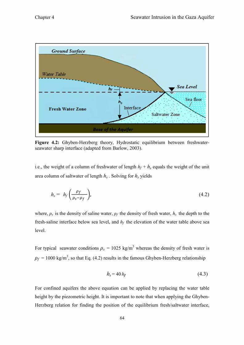
Chapter 4 Seawater Intrusion in the Gaza Aquifer
64
Figure 4.2: Ghyben-Herzberg theory, Hydrostatic equilibrium between freshwater-seawater sharp interface (adapted from Barlow, 2003).
i.e., the weight of a column of freshwater of length hf + hs equals the weight of the unit
area column of saltwater of length hs . Solving for hs yields
hs = hf ���
����� �, (4.2)
where, ρs is the density of saline water, ρf the density of fresh water, hs the depth to the
fresh-saline interface below sea level, and hf the elevation of the water table above sea
level.
For typical seawater conditions ρs = 1025 kg/m3 whereas the density of fresh water is
ρf = 1000 kg/m3, so that Eq. (4.2) results in the famous Ghyben-Herzberg relationship
hs = 40 hf (4.3)
For confined aquifers the above equation can be applied by replacing the water table
height by the piezometric height. It is important to note that when applying the Ghyben-
Herzberg relation for finding the position of the equilibrium fresh/saltwater interface,

Chapter 4 Seawater Intrusion in the Gaza Aquifer
65
one must require that the water table lies above sea level and that it is inclined toward
the coast. Without this condition, seawater would advance directly inland.
In fact, the Ghyben-Herzberg relationship is based on the hydrostatic conditions and,
thus, neglects the freshwater movement toward the sea. Therefore, in reality, the actual
interface should be located below that determined by Ghyben-Herzberg (Figure 4.3, left
panel). This difference in location is due to the effect of the seepage forces, resulting
from the freshwater movement, which create groundwater gradient towards the sea
(Kashef, 1977; 1982).
Bear and Dagan (1964a) investigated the validity of the Ghyben-Herzberg relationship
and, using the hodograph method, derived an exact solution for the shape and position
of the interface, for the case of a steady-state homogenous and isotropic confined
aquifer of constant thickness B (Figure 4.3, right panel). Their analysis shows that the
approximation is good, within an error of 5% for determining the depth of the interface
toe (point G), provided that (Bear, and Verrujit, 1987)
� � �
�� � > 8, (4.4)
where:
B, thickness of the aquifer,
K, hydraulic conductivity and
Q0, freshwater discharge to the sea, and
Ф, piezometric head above the toe, at point G (right panel of Figure 4.3).
In Figure 4.3, right panel, the exact (hodograph) and the Dupuit solutions (Ghypen-
Herzberg) are compared, which shows that, as the coast is approached, the depth of the
interface is greater than that predicted by the Ghyben-Herzberg relationship. Changes in
recharge conditions and increase of pumpage may disturb the movement of this
improved hodograph interface location further. In the case of unconfined aquifer, a

Chapter 4 Seawater Intrusion in the Gaza Aquifer
66
Figure 4.3: Left: Actually observed and Ghyben-Herzberg-determined salt/fresh water interface (British Geological Survey, 2002). Right: Piezometric head above interface toe in a confined aquifer (Bear and Dagan, 1964a).
seepage face develops above sea level, through which discharge of the freshwater into
the sea occurs (Figure 4.3, left panel).
4.2.2. Diffuse interface
As discussed, both the Ghyben-Herzberg and the improved hodograph method assume a
sharp interface. In reality, however, owing to a concentration gradient across the
salt/freshwater interface, salt is dispersed across the latter by molecular diffusion and
mechanical dispersion, i.e. hydrodynamic dispersion, so that a diffusive transition
(mixing) zone for the two fluids is established. In the context of the present study, this is
called the “diffuse interface approach”, and its analysis requires the solution of a
coupled density-dependent groundwater flow and solute transport problem (Sherif and
Singh, 1996). Thus, the idealized interfacial surface becomes a transition zone, as
shown in Figure 4.4, within of which the two water bodies merge and where the
concentration and the fluid density vary gradually from those of freshwater at the land
side to those of seawater at the sea side.
The approximation of diffuse interface has been wisely used to describe the behavior of
the seawater intrusion (e.g. Cooper, 1959; Bobba, 1993; Todd, 1980). Thus, Cooper
(1959) presented the existence of transition zone with on a very wide scale, therefore,
indicating that the approximation of a sharp interface may not be valid any longer.
Bobba (1993) stated that the thickness of the transition zone can vary from a few
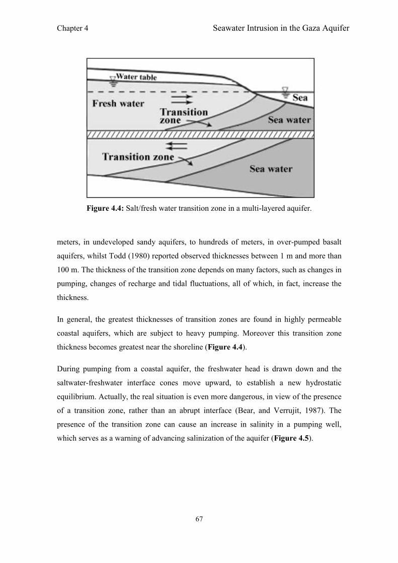
Chapter 4 Seawater Intrusion in the Gaza Aquifer
67
Figure 4.4: Salt/fresh water transition zone in a multi-layered aquifer.
meters, in undeveloped sandy aquifers, to hundreds of meters, in over-pumped basalt
aquifers, whilst Todd (1980) reported observed thicknesses between 1 m and more than
100 m. The thickness of the transition zone depends on many factors, such as changes in
pumping, changes of recharge and tidal fluctuations, all of which, in fact, increase the
thickness.
In general, the greatest thicknesses of transition zones are found in highly permeable
coastal aquifers, which are subject to heavy pumping. Moreover this transition zone
thickness becomes greatest near the shoreline (Figure 4.4).
During pumping from a coastal aquifer, the freshwater head is drawn down and the
saltwater-freshwater interface cones move upward, to establish a new hydrostatic
equilibrium. Actually, the real situation is even more dangerous, in view of the presence
of a transition zone, rather than an abrupt interface (Bear, and Verrujit, 1987). The
presence of the transition zone can cause an increase in salinity in a pumping well,
which serves as a warning of advancing salinization of the aquifer (Figure 4.5).

Chapter 4 Seawater Intrusion in the Gaza Aquifer
68
Figure 4.5: Saltwater upconing due to pumping from a transition zone.
4.2.3. Upconing of a saltwater/freshwater interface
The phenomena of saltwater ‘upconing’ describe the movement of saltwater from a
deep saltwater zone, upward into a shallower freshwater zone, in response to pumping,
from either single or multiple wells. Upconing may be caused by a single process or a
combination of different processes, which are widely known as upconing in coastal
aquifer and/or upconing inland aquifer (e.g. Todd, 1980; Zhou et al., 2005). In many
coastal aquifers, pumping freshwater from a well located above the transition zone
resulting upconing of the latter (Figure 4.5), so that salinizing of the pumped water
occurs, eventually forcing shut-off of the well.
In fact, saltwater intrusion does not only present a problem in coastal aquifers, but can
also occur inland aquifers which contain brines, that have entered the aquifer during
past geologic times. The upconing phenomena in such inland aquifers are not exactly
similar to the saltwater upconing, discussed above, as the dispersion is usually neglected
in the former case.
In general, when pumping takes place in wells screening above the interface, which are
often located within the freshwater zone, the underlying saltwater migrates vertically
upward and the interface forms an expanding shape of a cone (Figure 4.6).
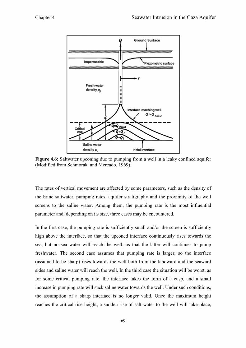
Chapter 4 Seawater Intrusion in the Gaza Aquifer
69
Figure 4.6: Saltwater upconing due to pumping from a well in a leaky confined aquifer (Modified from Schmorak and Mercado, 1969).
The rates of vertical movement are affected by some parameters, such as the density of
the brine saltwater, pumping rates, aquifer stratigraphy and the proximity of the well
screens to the saline water. Among them, the pumping rate is the most influential
parameter and, depending on its size, three cases may be encountered.
In the first case, the pumping rate is sufficiently small and/or the screen is sufficiently
high above the interface, so that the upconed interface continuously rises towards the
sea, but no sea water will reach the well, as that the latter will continues to pump
freshwater. The second case assumes that pumping rate is larger, so the interface
(assumed to be sharp) rises towards the well both from the landward and the seaward
sides and saline water will reach the well. In the third case the situation will be worst, as
for some critical pumping rate, the interface takes the form of a cusp, and a small
increase in pumping rate will suck saline water towards the well. Under such conditions,
the assumption of a sharp interface is no longer valid. Once the maximum height
reaches the critical rise height, a sudden rise of salt water to the well will take place,

Chapter 4 Seawater Intrusion in the Gaza Aquifer
70
which means a significant deterioration of the water quality in the well, so that it has to
be shut down. The critical rise height can be expressed in terms of the ratio of the
interface rise divided by the distance between the original location of the interface and
the bottom of the pumped well, and its analysis has been the subject of many studies.
Schmorak and Mercado (1969) give an approximate analytical solution for the upconing
height Z directly beneath a well, based on the Dupuit assumptions of in the Ghyben-
Herzberg theory:
� =� ��
2Л��( �� − ��) (4.5)
where, all of the quantities are shown in Figure 4.6, and are:
Z, new equilibrium elevation (L)
Q, pumping rate (L3/T)
d, distance from the base of the well to the initial (pre-pumping) interface (L)
ρf, density of fresh water (M/L3)
ρs, density of saline water (M/L3)
K, hydraulic conductivity (L/T).
Hydraulic model experiments have revealed that the relation in the above equation holds
only, if the rise height is limited (Kawabata, 1965). According to the field investigation
results, Dagan and Bear (1968) suggested that the interface will be stable for upconing
heights Z smaller than one third of d. substituting Z = 1/3*d in the above equation, the
maximum permissible pumping rate to impede salt entering the well is
Qmax ≤ 0.6 Л d 2 K (�� – �
� ) / �� (4.6)
A comparison of the rising of the saltwater to a pumping well for an abrupt interface
and for a transition zone is shown qualitatively in Figure 4.7.

Chapter 4 Seawater Intrusion in the Gaza Aquifer
71
Figure 4.7: Well water salinity curves for upconing of an abrupt interface and a transition zone (after Schmorak and Mercado, 1969).
From Figure 4.7 one may notice that with an abrupt (sharp) interface, assuming Q >
Qmax, the salinity of the well water increases later, but then more rapidly than is the case
when a transition zone is assumed. For Q < Qmax, no saltwater will reach the well for the
abrupt case; on the contrary, with a transition zone, there will be gradual invasion of
saline water into the well. The ultimate well-water salinity for both upconing
approaches lies then somewhere between that of fresh and the original saltwater,
wherefore the empirical data indicates that this final well-water salinity is only 5 to 8 %
of the original one (Schmorak and Mercado, 1969).
4.3. Evolution of seawater intrusion in the Gaza aquifer
In the Gaza strip, according to the hydrological data records on pump capacities reveals
that, over the years, the Gaza coastal aquifer has been overexploited from heavy
groundwater pumping to meet municipal and agricultural demands, where municipal
abstraction has been increased from about 12 x106 m3/yr, 35 x106 m3/yr, 55 x106 m3/yr
and 90 x106 m3/yr in years 1967, 1990, 2000 and 2010 respectively. Meanwhile, the
agriculture abstraction ranges between 90 x106 m3/yr and 80 x106 m3/yr (PWA, 2010a).
This increased demand cannot be balanced anymore by natural aquifer replenishment
from precipitation. As already discussed in Chapter 3, as a result of this over-

Chapter 4 Seawater Intrusion in the Gaza Aquifer
72
exploitation, the water levels across most of the coastal aquifer have dropped
significantly, with values going up to more than 12 m below the mean sea level in some
areas. Such large groundwater level declines have led to increased sea water intrusion
and a subsequent deterioration of the freshwater quality, as the chloride concentrations
have exceeded the safe drinking threshold value of 250 mg/l recommended by WHO
guidelines.
In fact, the available recharge in the Gaza aquifer is mainly due to the natural
replenishment by rainfall and other minor sources such as the agricultural and
wastewater return flow and the sub-ground lateral inflow from the eastern part of the
aquifer (see Chapter 6 for details).
In general, the average annual volume of rainfall is about 110-125 MCM, while the
potential evaporation in the Gaza strip is of the order of 1300 mm/yr. So it becomes
clear that the rejuvenation of water resources in the region is rather low and the
demands cannot be balanced anymore by natural aquifer replenishment from
precipitation, where the latter ranges between 42-48 MCM/yr (PWA/USAID, 2000a).
In particular, high rates of urbanization are considered the most influential on reducing
natural aquifer replenishment from precipitation. In fact, more than 40 % of total rain
water is discharged to the sea by natural surface run-off or pumping, in order to protect
the residential areas in the lower inland from flooding (Aish and De Smedt, 2004). In
the Gaza strip the percentage of urbanized area to the total area was estimated as 16 %
and 20 % in years 1998 and 2004, respectively, and, due to population growth, it is
expected to increase in the future, to reach 33% and 44.5% for the years 2015 and 2025,
respectively. This urbanization will lead to a decreased recharge rate from rainwater,
i.e., to an increase of the rainfall surface run-off, where the latter been estimated as 14.5
MCM (million cubic meters) in year 1998, and is expected to increase to 20 MCM, 35
MCM and 52 MCM for years 2005, 2015 and 2025, respectively (Al-Yaqoubi, 2007).
As a matter of fact, combination of overexploitation from the aquifer, the subsurface
lateral inflow of brackish groundwater from the east, return flow from irrigated lands,
and disposal of saline water from septic tanks and networks leakage have led to the
steeply increase of the salinization in the Gaza coastal aquifer in recent decades.

Chapter 4 Seawater Intrusion in the Gaza Aquifer
73
In order to understand the process of salinization in the Gaza aquifer, two approaches
are used which are based on the analysis of the groundwater time series data recorded
between 1935 and 2010 across the Gaza strip, conducted by the Palestinian Water
authority (PWA), ministry of agriculture (MoA), and the ministry of health (MoH). In
the first approach, the spatial patterns in the groundwater levels and the chloride
concentrations were analyzed. In the second approach, typical trends in the chloride
time series data for some wells were specified.
Before starting with the analysis process, it is important to define what is meant by
saline water and describe the degree of salinity as a first step to discriminate between
water salinity. The United States Geological Survey (USGS) suggested such terms,
which related to the degree of salinity as presented in Table 4.1.
Table 4.1: Terms describing degree of salinity as used by USGS (after Hem, 1970).
Description TDS (mg/l)
Fresh < 1000
Slightly saline 1000 – 3000
Moderately saline 3000 – 10000
Very saline 10000 – 35000
Brine > 35000
Drinking water standards established by the Environmental Protection Agency (EPA) in
1962 require that the drinking water should not contain more than 500 mg/l of total
suspended solids (TSS), and 1000 mg/l of total dissolved solids (TDS) both of which
are common measures of the salinity. Dissolved solids in natural waters primarily
include carbonates, bicarbonates, chlorides, sulfates, and phosphates, where all
dissolved salts change the physical and chemical nature of water. In fact, water becomes
salty to taste for most people, once the chloride concentrations exceed the safe drinking
threshold value of 250 mg/l, as recommended by WHO guidelines.

Chapter 4 Seawater Intrusion in the Gaza Aquifer
74
4.4. Historical water level and chloride concentrations in Palestine
In Palestine, hydrologic characteristics surveys were already carried out under the
British Government on Palestine between the period 1917–1948. Regular monitoring
throughout the region began in the early 1930s. Between October 1934 and September
1935 a survey of chloride concentrations and groundwater levels in wells were
conducted throughout the region. This survey included 397 wells in the coastal aquifer
in the vicinity of the Gaza strip, and 23 wells in the mountain aquifers in the vicinity of
the West Bank (British Government of Palestine, 1947a). These measurements showed
that the chloride concentration in some coastal areas were above 250 mg/l already at
that time (British Government of Palestine, 1947a, 1947b, 1948).
Presently, the Palestinian water authority (PWA) has established a data bank for
monitoring the water levels and chloride concentrations, with the incorporation of data
from the ministry of agriculture (MoA) and the ministry of health (MoH). The water
levels are measured monthly in the agricultural observation wells, whereas the ministry
of health (MoH) conducts chloride concentrations tests biannual in February and
October in the municipal monitoring wells.
4.4.1. Spatial patterns of groundwater levels
The characterization of the groundwater levels has been carried out using the available
date, recorded from years 1935 to 2010. In a first investigation, the year 1935 was
considered to reflect real steady-state conditions, as that time only a few wells were
pumping water, given that the population did not exceed 55,000 inhabitants in the whole
Gaza strip.
The two panels of Figures 4.8 shows the observed yearly groundwater levels in years
1935 and 1969. These observed hydraulic heads indicate that all the head isolines have
positive groundwater levels, i.e. the latter are laying above mean sea level. Moreover, as
the groundwater level contours are decreasing from east towards the coast, a natural
hydraulic gradient from inland (freshwater) to the coastline (saltwater) existed at that
time. Comparing the two groundwater isoline maps for the two historical years shows
that by year 1969 the groundwater levels had already declined by 8 m and 1 m in the

Chapter 4 Seawater Intrusion in the Gaza Aquifer
75
Figure 4.8: Contours map for groundwater levels at year 1935 (left) and at year 1969 (right) (Qahman and Larabi, 2005).
eastern and western parts, respectively, of the northern area, relative to those in year
1935. In contrast, the groundwater levels in the southern area of Gaza, had barely
changed over this 34-year long time period. As a matter of fact, after the cease fire line
in 1948, which resulted the occupation of Palestine, the population in the Gaza strip
increased tremendously, due to the influx of refugees from areas around the Gaza. Thus,
the population reached more than 80,000 inhabitants in year 1948 and increased to
about 455,000 inhabitants in 1967 (PCBS, 1998). As most of these incoming people
were concentrated in agglomeration in the north of Gaza (Jabalia Camp) which is the
most densely populated area in the Gaza strip, this has led to a tremendous increase in
the water demands and of the abstraction rate from the aquifer to satisfy the municipal
demand. In addition, with the development of agricultural areas starting in year 1967,
followed by extended irrigation activities, huge amounts of groundwater have been
extracted through the nearly 4000 agricultural and municipal wells, dug since that time
(see Chapter 3).
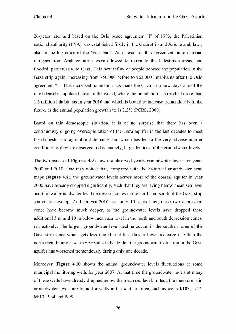
Chapter 4 Seawater Intrusion in the Gaza Aquifer
76
26-years later and based on the Oslo peace agreement "I" of 1993, the Palestinian
national authority (PNA) was established firstly in the Gaza strip and Jericho and, later,
also in the big cities of the West bank. As a result of this agreement more external
refugees from Arab countries were allowed to return to the Palestinian areas, and
flooded, particularly, to Gaza. This new influx of people boosted the population in the
Gaza strip again, increasing from 750,000 before to 963,000 inhabitants after the Oslo
agreement "I". This increased population has made the Gaza strip nowadays one of the
most densely populated areas in the world, where the population has reached more than
1.6 million inhabitants in year 2010 and which is bound to increase tremendously in the
future, as the annual population growth rate is 3.2% (PCBS, 2000).
Based on this demoscopic situation, it is of no surprise that there has been a
continuously ongoing overexploitation of the Gaza aquifer in the last decades to meet
the domestic and agricultural demands and which has led to the very adverse aquifer
conditions as they are observed today, namely, large declines of the groundwater levels.
The two panels of Figures 4.9 show the observed yearly groundwater levels for years
2000 and 2010. One may notice that, compared with the historical groundwater head
maps (Figure 4.8), the groundwater levels across most of the coastal aquifer in year
2000 have already dropped significantly, such that they are lying below mean sea level
and the two groundwater head depression cones in the north and south of the Gaza strip
started to develop. And for year2010, i.e. only 10 years later, these two depression
cones have become much deeper, as the groundwater levels have dropped there
additional 3 m and 10 m below mean sea level in the north and south depression cones,
respectively. The largest groundwater level decline occurs in the southern area of the
Gaza strip since which gets less rainfall and has, thus, a lower recharge rate than the
north area. In any case, these results indicate that the groundwater situation in the Gaza
aquifer has worsened tremendously during only one decade.
Moreover, Figure 4.10 shows the annual groundwater levels fluctuations at some
municipal monitoring wells for year 2007. At that time the groundwater levels at many
of these wells have already dropped below the mean sea level. In fact, the main drops in
groundwater levels are found for wells in the southern area, such as wells J/103, L/57,
M/10, P/34 and P/99.

Chapter 4 Seawater Intrusion in the Gaza Aquifer
77
Figure 4.9: Contours maps of groundwater levels for year 2000 (left) and 2010 (right).
Figure 4.11 depicts typical trends of the annual groundwater level time series for the
periods 1971-2010 for some monitoring wells located in the south and north of the Gaza
strip. From this figure, one may notice, that there are considerable drops in the water
levels from about 2.2 m above mean sea level (AMSL) to 1.0 m below mean sea level
(BMSL) between years 1971 and 1986. However, after year 1993, i.e., “Oslo I”, the
groundwater level declines have been even more precipitous and the heads have become
permanently negative since then, which means that the aquifer has been continuously
depleted since that time. The reasons for this very precarious aquifer development have
been stated above.
4.4.2. Spatial pattern of chloride concentrations
The characterization of the aquifer salinity has been carried out, using the available date
recorded from year 1935 to year 2010, thus showing the historical development of the
chloride concentrations for the years 1935, 1970, 2002 and 2010 respectively.
The two panels of Figure 4.12 show the observed yearly chloride concentration for year
1935 and 1970, respectively. As discussed one can assume that for year 1935, both
hydraulic heads and the salinity are in steady-state conditions. This figure indicate that

Chapter 4 Seawater Intrusion in the Gaza Aquifer
78
Figure 4.10: Average water levels for year 2007 at some of the monitoring wells in the Gaza strip.
Figure 4.11: Long-term decrease of annual water levels at some wells.
-12
-10
-8
-6
-4
-2
0
2
4
6
8
10
12
Wa
ter
Lev
el (
m)
Well ID
Water Level-2007
-12
-10
-8
-6
-4
-2
0
2
4
19
70
19
72
19
74
19
76
19
78
19
80
19
82
19
84
19
86
19
88
19
90
19
92
19
94
19
96
19
98
20
00
20
02
20
04
20
06
20
08
20
10
Ave
rage
wat
er le
vel
(m)
Year
Water level time series for some wells
P10P/99A/53

Chapter 4 Seawater Intrusion in the Gaza Aquifer
79
Figure 4.12: Chloride concentration maps for year 1935 (left) and 1970 (right) (Qahman and Larabi, 2005).
the observed salinity for year 1935 is normal across most of the aquifer area, as the
chloride concentrations range from less than 100 mg/l to more than 600 in the north and
south, respectively, except in the south-eastern area, where the salinity exceed 1000
mg/l already at that time, which is a consequence of the upconing of old geologic
formation brines originated at the Naqab (Negev) desert.
Between years 1935 and 1970, no considerable change in the chloride concentrations
can be observed. This might be due to the fact that within this period there was enough
water storage and the aquifer was balanced by natural replenishment of precipitation.
Due to the mentioned large population growth in recent decades, with an ever-
increasing demand for domestic and agricultural water, groundwater in the region has
been overexploited over the years. This has led to excessive reductions in yields and
deterioration of ground water quality i.e. increase of saltwater intrusion. This can be
clearly seen from the two panels of Figure 4.13 which depict the aquifer salinization for
years 2002 and 2010. Whereas the chloride ion concentrations for year 2002 vary from
less than 250 mg/l to 500 mg/l in the sand dune areas in the north and southwestern area
of the Gaza strip, where the natural recharge by infiltration through the sand dune has a

Chapter 4 Seawater Intrusion in the Gaza Aquifer
80
Figure 4.13: Chloride concentration maps for year 2002 (top) and 2010 (bottom) (PWA, 2003; CMWU, 2010).
Chapter 4 Seawater Intrusion in the Gaza Aquifer
81
positive impact as it prevents the aquifer from salinization, the salinity are increased
along the coastal line of the aquifer, where they go from 700 mg/l to more than 1000
mg/l, particularly, in the central part of Gaza. This is clearly an indication that the
aquifer has become to be invaded by seawater in this area. This is primarily due to the
high rate of groundwater abstractions which has taken place here over the long term,
accentuated by the limited sub-surface inflow from the east.
Moreover, the salinity has increased steeply between years 2002 and 2010, as by that
time the seawater intrusion process has practically encompassed most of the aquifer
area, with chloride concentrations exceeding 1500 mg/l and reaching 3000 mg/l in some
places, especially, in the south-eastern area of the Gaza strip, where Israeli irrigation
activities and the named upconing phenomena may play a major adverse role.
About 195 municipal wells distributed across the Gaza strip’s governorates were used to
monitor the chloride concentrations in year 2010. These were measured biannual in
February and October by the ministry of health (MoH). The results are shown in Figure
4.14. The data from these 195 monitoring wells indicates that about 73 % of all
monitoring wells have chloride ion concentrations increased beyond the WHO-endorsed
250 mg/l drinking water standard. Moreover, 59 % of these wells have chloride
concentrations above 500 mg/l - with some of them having values of more than 7000
mg/l, particularly, in the Gaza governorate. And as already mentioned, the chloride
concentrations are less than 250 mg/l in the sand dune areas in the north and northwest
of the Gaza strip, which have high recharge coefficient of about 70%.
4.5. Typical trends in the chloride time series
4.5.1. Average trends
In Figure 4.15, the 1970-2010 time series of the average yearly chloride concentrations
of all monitoring wells across the Gaza strip is presented. It is obvious that, between
year 1970 and 1983, the total of all monitoring wells still had chloride concentrations
that were within the WHO- 250 mg/l drinking water standard. However, after year 1983
the chloride concentrations have continuously being increasing above that level, to
reach a value more than 800 mg/l by year 2010, which by now should even be higher.

Chapter 4 Seawater Intrusion in the Gaza Aquifer
82
Figure 4.14: Frequency distribution of 195 chloride monitoring wells across Gaza with frequencies of wells that have critical chloride concentrations > 250mg/l in year 2010.
Figure 4.15: 1970-2010 average annual chloride concentration time series for Gaza.
46
66
3134
20
10 (22%)
62 (94%)
28 (90%) 29 (85%)
13 (65%)
0
10
20
30
40
50
60
70
North Gaza Middle Kh-Younis Rafah
No
. of
Wel
ls
Gaza Strip Governorates
no. Of wellsno. of wells with Cl >250 mg/l
Year
0
100
200
300
400
500
600
700
800
900
1970
1972
1974
1976
1978
1980
1982
1984
1986
1988
1990
1992
1994
1996
1998
2000
2002
2004
2006
2008
2010
Ch
lori
de
co
nc
en
tra
tio
n (
mg
/l)
Avg. Chloride Conc. (mg/L) Over Municipal Wells
Avg. Cl (mg/L)
WHO (250 mg/l)
Chapter 4 Seawater Intrusion in the Gaza Aquifer
83
In the following two sub-sections steady-state and transient chloride concentration time
series across the Gaza region will be explored in some more details.
4.5.2. Steady-state chloride concentrations
Steady-state salinity mainly exists in the north and south-west of the Gaza strip,
particularly, in the sandy dune areas, but are also found in silt-clayey area. Figure 4.16
presents the steady-state chloride condition of well C-20, which is located at Beit-
Hanoun in the north-east area of the Gaza strip and about 8 km away from the shore
line. The average measured chloride concentration between the year 1970 and 2007 is
247 mg/l, i.e., it is within the WHO-endorsed 250 mg/l drinking water standard. This
can be interpreted by the fact that the extent of seawater intrusion does not reach the
distance of that well from the sea shore line. Meanwhile, after year 2008, the chloride
concentration at that well has increased to 290 mg/l, which, to some extent, is still
acceptable.
4.5.3. Transient chloride concentration increases
Figure 4.17 shows the continuously ongoing increase in chloride concentration in well
E-154, which is located at the north of the Gaza city, and only about 1700 m away from
the sea shore. One can conclude from this figure that for the 1987-1999 period, the
increase in the salinity has been gradual, as the chloride concentration ranges between
67 mg/l and 190 mg/l, i.e., it is still under the WHO-endorsed 250 mg/l drinking water
standard. In contrast, from year 2000, the salinity has been raising sharply, to reach a
value of more than 3600 mg/l by year 2010. This mean that well E-154 had been
severely affected by seawater intrusion over the last decade, which means, at the same
time, that the northwest part of the Gaza governorate has also been affected by seawater
intrusion.

Chapter 4 Seawater Intrusion in the Gaza Aquifer
84
Figure 4.16: Time series (steady-state) of average annual chloride concentration for well C-20.
Figure 4.17: Time series (transient) of annual chloride concentration for well E-154.
Well C-20
0
50
100
150
200
250
300
350
19
70
19
72
19
74
19
76
19
78
19
80
19
82
19
84
19
86
19
88
19
90
19
92
19
94
19
96
19
98
20
00
20
02
20
04
20
06
20
08
20
10
Cl
(mg
/l)
Year
CL (mg/l)
WHO (250 mg/l)
Well E-154
0
500
1000
1500
2000
2500
3000
3500
4000
19
86
19
88
19
90
19
92
19
94
19
96
19
98
20
00
20
02
20
04
20
06
20
08
20
10
Cl
(mg/
l)
Year
CL (mg/l)WHO (250 mg/l)

Chapter 4 Seawater Intrusion in the Gaza Aquifer
85
4.6. Summary
In this chapter the hydrodynamic characteristics and the mechanisms of salinization
processes, in general, have been defined. In particular, the historical evolution of
saltwater intrusion in the Gaza aquifer over the last decades has been presented.
Hydrological data analyses of the groundwater time series recorded between 1935 and
2010 across the Gaza aquifer have been used for that purpose. The results show that
over the last two decades, especially, the groundwater situation in the Gaza region has
become more than disastrous, both from a quantitative and a qualitative point of view,
and measures to forestall further future deteriorations, or even for remedy, are urgently
needed. To do this properly, computer modelling which allows the accurate simulation
of the dynamics of the groundwater system, in response to various hydrological,
meteorological, and human impact factors, is the indispensable tool. This is the focus of
the following chapters.

Chapter 5 Artificial Neural Network (ANN)
86
Chapter 5 : Groundwater Level Modeling and Forecasting using the Statistical Method of Artificial Neural Networks (ANN)
5.1. Introduction
Seawater intrusion in coastal aquifer can be characterized by many factors, such as:
varying spatial location, recharge, abstraction rate and others. As a first step to approach
the problem, a better understanding of the whole groundwater dynamics of the whole
Gaza coastal aquifer is needed. Also, in the primary studies, it is important to include all
factors that may have an effect on groundwater salinity. To do this properly, computer
modelling of groundwater flow and transport has nowadays become a powerful tool for
understanding and analyzing the hydrology of aquifers and various other aspects of
subsurface flow dynamics and numerous models are available for that purpose (e.g.
Anderson and Woessner, 1992; Kresic, 1996). These models usually look for a
numerical solution of the fundamental differential equations that describe the physics of
flow and transport in a porous subsurface media, after the latter has been put into a
conceptual model form, using geological and hydro-geological information on the
aquifer system.
In spite of, up-to-date, uncountable applications of numerical groundwater modeling to
all kind of groundwater aquifer systems across the world, including the Gaza coastal
aquifer (Sirhan and Koch, 2012b; Sirhan and Koch, 2013a), mostly with the goal to
predict the behaviour of groundwater flow or levels in an aquifer under time-varying
external stresses, such as, for example, increased pumping or changing aquifer recharge
due to climate change, practical groundwater modelling can still be a formidable task.
This is less due to an inadequate mathematical translation of the deterministic physical
flow system, but more due to an insufficient description of the latter itself, as geological
and hydro-geological data on the aquifer, as well as groundwater data, is often missing
or fraught with errors. Eventually, this may lead to a situation where a groundwater
model cannot be calibrated properly anymore, so that its predictive power must be put
into question. To overcome some of these deficiencies of physically-based numerical
models in poorly constrained real applications, alternative optimization methods have

Chapter 5 Artificial Neural Network (ANN)
87
been proposed over the last two decades. One of the common methods is artificial
neural networks (ANN), which has been used widely over this period on groundwater
applications, which is of interest in the present study, ANN has also become a method
of choice over the last decade (e.g. Coulibaly et al., 2001; Mao et al., 2002;
Daliakopoulos et al., 2005; Lallahem et al., 2005; Coppola et al., 2005, 2007; Affandi
and Watanabe, 2007; Feng et al., 2008; Seyam and Mogheir, 2011; Jalalkamali and
Jalalkamali, 2011). Thus, Coulibaly et al. (2001), Mao et al. (2002) and Coppola et al.
2003, applied ANN to predict groundwater levels under variable weather conditions,
whereas Daliakopoulos et al. (2005), Lallahem et al. (2005), Coppola et al. (2005;
2007) and Feng et al. (2008) did the same, but looked in particular for the effects of
pumping, i.e. groundwater abstraction rates. Affandi and Watanabe (2007) used ANN to
forecast groundwater level fluctuations for one day ahead, using time-lagged water
levels as input. ANN has been firstly applied to the Gaza coastal aquifer by Seyam and
Mogheir (2011) who looked for relationships between various hydrogeological
variables and the prevalent groundwater salinity in the area. Unlike in the afore-
mentioned study, ANN is used in this study as a new alternative tool to understand the
dynamic groundwater flow behavior in the Gaza coastal aquifer. More specifically,
ANN–relationships between (dependent) groundwater levels and various (independent)
hydrogeological variables will be established which can then be used to predict future
groundwater head fluctuations under varying hydrological, meteorological or other
human impact conditions.
In this chapter, the ANN-model has been applied to the Gaza coastal aquifer with seven
predictors independent variables in order to describe the effects of hydrological,
meteorological and human factors on the dynamic aquifer system over the period 2000-
2010 and to investigate and understanding the more influential parameters on the
behavior of the Gaza aquifer. This approach is considered as initial step towards
implementation a proper set-up of physically-based numerical model. Therefore, the
results turns out by the final ANN-model are used as a complement to a classical
(deterministic) groundwater model as implemented in Visual MODFLOW-model,
which may improve the understanding of complex groundwater system and improve the
simulation of groundwater management in the highly overstressed Gaza coastal aquifer
(see Chapter 6).

Chapter 5 Artificial Neural Network (ANN)
88
5.2. ANN modeling approach
5.2.1. Data and selection of independent input variables used in the ANN model
For a successful ANN-model implementation, the availability of good data both in
quantity and quality is necessary (Smith and Eli, 1995; Tokar and Johnson, 1999).
Gathering such data is the first step in the development of an ANN-model.
In the present study the data required has been obtained from the ministry of agriculture
(MoA) in the Gaza strip and it consists of various sets of groundwater time series data,
namely, yearly groundwater levels recorded at about 70 wells, mostly municipal wells
distributed across all the Gaza strip (Figure 5.1) over the 11-year time span 2000-2010
and to the extent that they are available pumping rates. Since the raw data often
contained missing records, or was afflicted by all kind of instrumental and human
errors, it had to be cleaned and filtered properly, before it could be used in the ANN-
model training. It is necessary to deal with consistent data set of patterns containing
values for input and output variables. The next step in the set-up of ANN-model is the
selection of possible significant independent input variables which will affect the
dependent output variable (groundwater levels). In the present ANN-model, these are,
namely, the groundwater abstraction and the recharge from rainfall and surface water. A
corroboration of this fact was obtained from correlation analyses of the (11 years x 70
wells = 770) long output column vector of the output (head) data with the two columns
of the input matrix (abstraction and recharge), the results of which indicated, indeed,
that these two variables serve well as the two main independent variables in the ANN-
model (Sirhan and Koch, 2012a).
Nevertheless, an additional subset of other possible independent input variables was
tested to serve as influential predictors in the ANN-model. The latter were chosen based
on knowledge about the physics and hydrogeology of the groundwater system,
literatures and gained either from experience.

Chapter 5 Artificial Neural Network (ANN)
89
Figure 5.1: Distribution of the pumping wells across the Gaza strip.
Eventually, in addition to the ground water extraction rate Q, and the groundwater
recharge from rainfall R, five more predictor input variables, namely, initial ground
water level WLi, hydraulic conductivity K, distance of the abstraction wells from the
shore line Dshore, depth to the well screen Dscreen and well-density Wdens were selected in
the initial ANN-model to predict some final output water levels WLf .
In Table 5.1 the basic descriptive statistical properties for the seven independents
variables, namely, minimum, maximum, mean, median, std. deviation and coefficient of
variation are summarized.

Chapter 5 Artificial Neural Network (ANN)
90
Table 5.1: Descriptive statistics for the independent observed variables used in the ANN-model.
Variable Unit Min. Max. Mean Median Std.
Dev.
Coef.
Variat.1
Initial water level WLi m -12.8 10.73 -1.45 -1.38 3.11 -2.14
Abstraction rate Q m3/hr 0 240.9 75.53 64.64 61.1 0.81
Recharge rate R mm/m2/month 6.57 80.15 26.93 21.15 15.98 0.59
Hydraulic conductivity K m/d 15 40 31.21 30 8.97 0.29
Distance from shore Dshore Km 0.8 10.19 3.63 3.1 2.11 0.58
Distance to well screen Dscr. m 8.95 122.3 64.54 65.6 30.13 0.47
Well density Wdens No./km2 4.9 19.32 10.5 9.96 5.19 0.49
1defined as the ratio of the standard deviation to the mean
5.2.2. General formulation of the ANN-model
An ANN-model describes a general functional relationship,
Y = f (X)
(5.1)
between some input (predictor) matrix X consisting of m independent variable vectors
x1, x2, . . . , xm; and a dependent (predictand) output variable vector Y. Independent
variables are those that are manipulated, whereas dependent variables are measured or
registered. Goal of ANN- modeling is then the quantification of the function f during
the so-called training phase, so that new predictands can be forecast from other input
variables in the subsequent prediction phase.
As discussed in the previous section, the output variable vector Y in Eq. (5.1) consists
here of the unknown final water levels WLf, which are supposed to depend on seven
input parameter (column) vectors x1, x2, . . . , x7 of X, namely, WLi, Q, R, K, Dshore,
Dscreen., and Wdens. Using these variables, Eq. (5.1) is then reads
��� = � (���, �, �, �, ��ℎ���, �������, ��������)
(5.2)
Chapter 5 Artificial Neural Network (ANN)
91
As will be shown during the optimization of the ANN-model in the following sections,
some of these seven independent variables turn out to be not significant for the
prediction and can thus be omitted in the final ANN-model.
5.2.3. Architecture and optimization of the ANN-model
The basic concept of an artificial neural network (ANN) is derived from an analogy
with the biological nervous system of the human brain and how the latter processes
information through its millions of neurons interconnected to each other by synapses.
Borrowing this analogy, an ANN is a massively parallel system composed of many
processing elements (neurons), where the synapses are actually variable weights,
specifying the connections between individual neurons and which are adjusted, i.e. may
be shut on or off during the training or learning phase of the ANN, similar to what is
happening in the biological brain.
However, here the analogy of a technical ANN with the real brain already comes to an
end, as the architecture of the former is inevitably much simpler than that of the latter.
Thus, the neurons in an ANN are usually set-up in consecutive layers, the so-called
perceptrons, and information is going from the input nodes (neurons) in the first layer
across one or several intermediate or hidden layers to the output nodes in the output
layer (see Figure 5.2). If this pure forward passing of information is not accompanied
by extra cycles or loops within one layer, which actually may happen in a biological
brain one speaks of a feed-forward neural network. It is the simplest form of an ANN
and, for this reason, also the most commonly used in practice.
Although the number of hidden layers between the input and output perceptrons could,
in theory, be arbitrarily increased, to better mimic the functioning of the biological brain
in the case of which one also speaks of a multiple layer perceptron (MLP) network, the
ensuing exponential increase of the neurons and, more so, of the synapses (the
activation weights), makes such an approach totally impractical. Thus, most of the ANN
used in practice are using only a few, or sometimes even none, hidden layers. For each
application the most suitable architecture of the ANN is then determined by trial and
error in the initial testing phase.

Chapter 5 Artificial Neural Network (ANN)
92
Figure 5.2: Architecture of the initial ANN-model network with input layer, one hidden layer and output layer.
Figure 5.3: Backpropagation of error signals from output to hidden and input layers to update the weights.
In the training or learning phase of the ANN, using known information at the input and
output neurons, the activation weights of the synapses connecting neurons in different
layers are computed (see Figure 5.2). This amounts to iteratively correcting initially
estimated values of the weights, until the error between observed and predicted output is
minimal. Mathematically this is equivalent to solving a multi-objective minimization or
optimization problem and can be done, for example, by classical gradient methods, as
they have been known for many decades in the field of general mathematical

Chapter 5 Artificial Neural Network (ANN)
93
optimization (e.g. Gill et al., 1981). These methods are using the gradient of the error
cost function to move step by step towards its minimum.
In the ANN-community this approach is also known as error back-projection, which
means that errors occurring at a particular stage of the iteration process at the output
layer are back-propagated consecutively through the various perceptrons of the ANN to
compute corrections of the unknown activation weights (Figure 5.3).
Similar to classic gradient optimization the derivative of the error cost function must be
computed which means that the activation weights must derivable. For this reason the
latter are set up in the form of a monotonously increasing activation function. In most
ANN applications the so-called sigmoid function is used.
In spite of the widespread applications of the feed-forward MLP–ANN with error back-
projection, as described above, the method may be prone to errors and instabilities for
multidimensional problems, as it will often, likewise to the classical gradient method,
find only a local, but not a global minimum of the error cost function. This means that
the final optimal model will depend somehow on the initial conditions. To overcome
partly this deficiency, radial basis functions (RBF), which have some kind of a distance
criterion built in with respect to a centre, have been proposed, instead of the sigmoid
functions to transfer information across the hidden layers. Usually only one hidden layer
is used in such a RBF-ANN- network and the non-linear RBF activation function
commonly taken to be a Gaussian is only applied to this layer, whereas the final transfer
to the output layer is done in linear manner.
The various procedure discussed above for setting up an ANN-model can be
implemented either in a mathematical, such as the neural network toolbox of MATLAB,
or a statistical computational environment, like neural network STATISTICA. The latter
is used in this study STATISTICA is a comprehensive, integrated data analysis,
graphics, and database management which is used in a wide range of engineering
applications. Although the STATISTICA ANN-module operates somewhat under a
black box the user can select numerous tuning knobs to gear the program through the
various steps of ANN- model testing, learning, validation and prediction.

Chapter 5 Artificial Neural Network (ANN)
94
5.3. ANN-simulation results
5.3.1. Initial ANN-model
5.3.1.1. General characteristics and statistical performance
The initial ANN-model trials were formatted using all seven input variables (neurons) in
Eq. (5.2). From the 770 observed water levels, half (=386) were selected randomly for
the training of the model and the remaining half of the data was divided in two equal
sets; one for validation and the other for testing (prediction).
Practically, the training of the network consists of a forward propagation of the inputs
and a backward propagation of the error (Figure 5.3). In the forward procedure, the
effect of an applied activity pattern at the input layer is propagated through the network
layer by layer. During network training, the data are processed through the ANN, and
the connection weights are adjusted adaptively, until a minimum acceptable error is
achieved between the predicted and the observed output. Both, multilayer perceptron
(MLP) and radial basis function (RBF) ANN models were examined. Many different
models with different numbers of hidden layers and different activation functions were
tested. To that avail an intelligent problem solver (IPS) to determine the model
constraints which include optimization time, network type and the number of hidden
units, and paying attention to the relationships among all input variables was developed.
Surprisingly, and disproving somewhat the explanations afore-mentioned in the
previous section, the classical MLP network with a sigmoid activation function turned
out to be better than a RBF- network. For this reason the latter ANN-option was not
followed up further.
The characteristics of the initial MLP-ANN-model network are presented in Figure 5.2
and summarized in Table 5.3. This network has three perceptron layers, i.e. an input
layer of 7 neurons, representing the variables in Eq. (5.2), a hidden layer with 8 neurons,
and one output layer with one neuron (the final water level). From the table one may
note that the performance measure defined as the ratio of the standard deviation of the
predictions to that of the observations for this network have low values for all three
ANN-steps, i.e. training, validation and testing. Also, Table 5.2 provides further

Chapter 5 Artificial Neural Network (ANN)
95
characteristics of the selected ANN network. Thus, the notation BP100, CG20, CG40b
in the last column indicates that one hundred passes of back-propagation, followed by
twenty and forty epochs of conjugate gradient descents have been used for optimizing
this model. More details of the statistical results for this initial ANN-model are provided
in Table 5.3, where various statistical indicators of the ANN-model simulations, some
of which are discussed further in the following paragraphs for the training, validation
and test phases are listed individually.
Table 5.2: Performance measures1 for the initial ANN- model
Profile Train.
perf.
Valid.
perf.
Test
perf.
Train.
error [m]
Valid.
error [m]
Test
error [m] Training/Members
MLP 7:7-8-1:1 0.217 0.318 0.286 0.023 0.031 0.026 BP100,CG20,CG40b
1defined as the ratio of the standard deviation of the ANN-predictions to that of the observations
Table 5.3: Statistics of observed and simulated water levels for the initial ANN- model.
Initial ANN model (3-MLP)
Statistical indicator
Mean data [m]
sd- data [m]
Mean error [m]
sd- error [m]
MAE1 [m]
sd- ratio2
Correlation coefficient
Overall model -1.671 3.329 0.016 0.859 0.572 0.258 0.966
Training data set -1.666 3.525 -0.017 0.765 0.543 0.217 0.976
Validation data set -1.620 3.237 0.055 1.030 0.635 0.318 0.948
Test data set -1.732 2.980 0.047 0.854 0.571 0.286 0.958
1defined in Eq. (5.3)
2defined as the ratio of the standard error of the ANN-model (sd error) to that of the data (sd data) and
corresponds to the performance measure in Table 5.2.

Chapter 5 Artificial Neural Network (ANN)
96
Figure 5.4: Simulated versus observed water level for the initial ANN- model.
In Figure 5.4 the simulated water levels obtained for the optimal initial ANN-model are
plotted against the observed water levels. In addition, the fitted linear regression line is
shown. As both the slope of this line and the correlation coefficient R (=0.966), the
latter being equal to the square root of R2, the coefficient of determination, are close to
one, the performance of this initial ANN- model can be considered as very good.
This R-value using all the data is to be compared to those obtained separately for the
training, validation (selection), and testing phases. The correlation coefficients are listed
in Table 5.3 and are 0.976, 0.948, and 0.958, respectively.
Predicted and observed water levels for the 70 well are shown for years 2000, 2005 and
2010 in the three panels of Figure 5.5. One may notice a good agreement between the
two for all these three years.
y = 0.931x - 0.098R = 0.966
-12
-8
-4
0
4
8
12
-12 -8 -4 0 4 8 12
Sim
ula
ted
WL
(m
)
Observed WL (m)

Chapter 5 Artificial Neural Network (ANN)
97
Figure 5.5: Initial ANN-simulated and observed water levels at the various wells for years 2000 (top), 2005 (middle) and 2010 (bottom).
-10
-6
-2
2
6
10
14
10 20 30 40 50 60 70
Wa
ter
lev
el (
m)
Well no.
Obs.WL Pred.WLYear-2000
-10
-6
-2
2
6
10
14
10 20 30 40 50 60 70
Wat
er le
vel
(m)
Well no.
Obs.WL Pred.WLYear-2005
-20
-15
-10
-5
0
5
10
15
10 20 30 40 50 60 70
Wat
e r le
vel
(m)
Well no.
Obs.WL Pred.WLYear-2010

Chapter 5 Artificial Neural Network (ANN)
98
5.3.1.2. Sensitivity analysis
A sensitivity analysis can provide information on the usefulness and significance of
individual input variables in the ANN-model (STATISTICA 7 manual, 2004). The
sensitivity of an independent input variable xi is normally measured by the ratio of the
change of the model output ΔY (see Eq. 5.1) to a change Δxi of this input variable.
Another measure which is also sometimes used in statistical inference, namely, in
stepwise regression, is to compare the mean squared error (MSE) between observed and
predicted datum for the two cases when a particular variable xi is included or not
included in the model. In ANN- applications it has been more common to use the mean
absolute error MAE instead, defined as
MAE = 1/n*∑ |Yiobs - Yi
sim | (5.3)
where Yiobs and Yisim is the observed and ANN-simulated datum, respectively, and n is
the number of observations. The sensitivity of the ANN-model to a particular variable is
then computed (e.g. Coppola et al., 2003; Feng et al., 2008) based on the ratio of the
MAE when a particular variable is not included in the model to that when it is included,
i.e.
Ratio = ���� ������� ��������� ���������
��� ���� ��� ��������� ��������� (5.4)
Under normal situations the MAE in the nominator of Eq. (5.4) is larger than that in the
denominator, since the omission of a particular variable will usually deteriorate the
performance of the ANN-model, i.e. the MAE will be increased. This means also that
the more important an input variable is in the ANN-model, the higher than one is the
ratio in Eq. (5.4). Thus, the size of the ratio allows a ranking of the importance of each
variable, relative to all other variables. Meanwhile, a ratio of less than 1 will also
indicate that the elimination of that input variable actually increases the ANN-model
accuracy.
In the practical sensitivity study, a total of fifteen ANN-models were analyzed, whereby
a single input variable out of the originally seven in the initial model (see Eq. 5.2) was

Chapter 5 Artificial Neural Network (ANN)
99
excluded one by one, and the corresponding error ratio is computed. These are listed in
Table 5.4 for the training phases for the 15 ANN-models tested, together with the mean
error ratio. From the ranking of the latter, the relative importance of the seven different
input parameters is inferred. The last row of Table 5.4 then indicates that the two
independent variables of depth to well-screen Dscreen and hydraulic conductivity K are
the least-influential variables affecting the final groundwater levels WLf, as they have
the small error ratios. An additional correlation analysis showed furthermore that these
two variables are only lowly correlated with the observed water levels WLf which
provides additional evidence that they can be safely ignored in the build-up of an
optimal ANN- model.
Table 5.4: Ratios of the MAE with ranking obtained during the sensitivity analysis for the various initial ANN- models during training.
Model no. WLi Q R K Dshore Dscreen Wdens
1 3.675 1.013 1.006 1.004 1.023 1.017 1.055
2 3.82 1.025 1.017 1.004 1.001 1.001 1.014
3 3.76 1.021 1.026 1.005 1.04 1.006 1.016
4 3.83 1.014 1.017 1.003 1.015 1.003 1.01
5 3.7 1.023 1.047 1.029 1.024 1.011 1.053
6 3.67 1.007 1.027 1.008 1.012 1.001 1.021
7 3.61 1.024 1.031 1.001 1.025 1.003 1.015
8 3.7 1.025 1.024 1.05 1.07 1.019 1.077
9 3.788 1.016 1.058 1.009 1.103 1.016 1.017
10 3.82 1.014 1.035 1.01 1.016 1.014 1.048
11 3.66 1.027 1.025 1.018 1.066 1.005 1.019
12 3.69 1.029 1.019 1.01 1.041 1.015 1.031
13 3.816 1.014 1.07 1.032 1.045 1.023 1.031
14 3.768 1.006 1.02 1.06 1.008 1.01 1.024
15 3.61 1.005 1.079 1.015 1.054 1.007 1.046
Mean error ratio
3.728 1.0175 1.033 1.017 1.036 1.01 1.032
Rank 1 5 3 6 2 7 4
Consequently, a new training of the network has been carried out in the following
section where only the retained five input variables, classified as important, are
incorporated in the model.

Chapter 5 Artificial Neural Network (ANN)
100
To conclude this section, the MAE- ratios of the overall initial ANN- model, i.e. using
all data, are listed in Table 5.5, together with the corresponding ranks of the influences
of the 7 input variables. This table corroborates the results of Table 5.4 with regard to
the selection of the 5 most influential in the set-up of the final ANN- model.
Table 5.5: Error ratio and rank for the seven input variables in the initial ANN-model.
Independent variable
WLi Q R K Dshore Dscreen Wdens.
Error ratio 3.82 1.025 1.017 1.004 1.013 1.001 1.014
Rank 1 2 3 6 5 7 4
5.3.2. Final ANN-model
5.3.2.1. General characteristics and statistical performance
Based on the sensitivity ranking of the seven input parameters used in the initial ANN-
model (see Table 5.5), the final neural network models were formatted employing only
the five input variables (neurons) WLi, Q, R, Dshore and Wdens..
Similar to the initial ANN- model, in this final ANN-model test series the 770 observed
output data (neurons) were divided randomly into three groups; a first one with 386 data
cases for training, a second one with 192 data for validation, and a third one with the
remaining 192 cases for testing (prediction). Also both MLP and RBF–models were
executed again and compared to each other.
The best network performance was attained with a four-MLP network, i.e. with two
hidden layers (perceptrons) between the input and output layer, and using a sigmoid
activation function in between these layers. More specifically, the input layer has 5
neurons, representing the specified input variables, a first hidden layer with 30 neurons,
a second hidden layer with 20 neurons and the final output layer with one neuron,
representing the output groundwater levels (Figure 5.6).

Chapter 5 Artificial Neural Network (ANN)
101
Figure 5.6: Architecture of the final ANN- model network with input layer, two hidden layers and output layer.
The performance characteristics of this final ANN-model are summarized in Table 5.6
and may be compared with those of the initial ANN-model listed in Table 5.2. From
these numbers one can deduce that the final ANN-model works better than the initial
one for the validation and testing phases. Also, Figure 5.7 indicates that this final ANN
fits the observed output very well, with a correlation coefficient R=0.969 for the
regression line between simulated and observed water levels. The corresponding R-
values for the training, validation and test set are 0.971, 0.970 and 0.965, respectively
(Table 5.7). As these R-values are more or less identical to the ones of the initial ANN-
model (Table 5.3), the advantage of this final ANN-model may not become
immediately clear. However, as this final model has been obtained with a smaller
number of input parameters than the initial one (5 against 7, respectively), it abides
better by the rule of parsimony, which is an important selection criterion in statistical
estimation.
The groundwater levels simulated with this final ANN-model are shown for the years
2000, 2005 and 2010, in the three panels of Figure 5.8. Similar to the initial ANN-
model (Figure 5.5), a very good agreement of the modeled and the observed water
levels is also noticed for this final ANN-model.

Chapter 5 Artificial Neural Network (ANN)
102
Figure 5.7: Simulated versus observed water levels for final ANN-model.
Table 5.6: Performance measures (for definition see Table 5.2) for the final ANN- model
Profile Train. perf.
Valid. perf.
Test perf.
Train. error [m]
Valid. error [m]
Test. error [m]
Training/Members
MLP 5:5-30-20-1:1
0.240 0.243 0.261 0.024 0.025 0.027 BP100,CG20,CG27b
Table 5.7: Statistics of observed and simulated water levels for the final ANN- model.
Final ANN- model (4MLP)
Statistical indicator
Mean data [m]
sd- data [m]
Mean error [m]
sd- error [m]
MAE
[m]
sd- ratio
Correlation coefficient
Overall model -1.635 3.34 0.027 0.829 0.552 0.248 0.969
Training data set -1.771 3.281 0.004 0.789 0.543 0.240 0.971
Validation data set -1.429 3.366 0.005 0.818 0.529 0.243 0.970
Test data set -1.705 3.373 0.071 0.881 0.584 0.261 0.965
y = 0.942x - 0.074R = 0.969
-12
-8
-4
0
4
8
12
-12 -8 -4 0 4 8 12
Sim
ula
ted
WL
(m
)
Observed WL (m)

Chapter 5 Artificial Neural Network (ANN)
103
Figure 5.8: Final ANN-simulated and observed water levels at various wells for years 2000 (top), 2005 (middle) and 2010 (bottom).
-8
-4
0
4
8
12
10 20 30 40 50 60 70
Wa
ter
lev
el (
m)
Well no.
Obs.WL Pred.WLYear-2000
-15
-10
-5
0
5
10
15
10 20 30 40 50 60 70
Wat
e r le
vel
(m)
Well no.
Obs.WL Pred.WLYear-2005
-20
-15
-10
-5
0
5
10
15
10 20 30 40 50 60 70
Wat
e r le
vel
(m)
Well no.
Obs.WL Pred.WL Year-2010

Chapter 5 Artificial Neural Network (ANN)
104
5.3.2.2. Response graphs and response surfaces
Eq. (5.2) may be viewed upon as an m-dimensional hypersurface of the response
variable final water level WLf, as a function of the m independent input variables of the
ANN-model. For an approximate visualization of such a hypersurface either one-
dimensional response graphs or two-dimensional response surfaces may be used.
5.3.2.2.1. Response graphs
Response graphs represent a one-dimensional slices through the hypersurface along the
direction of one independent variables with the remaining ones hold constant. Figure
5.9 shows the response graphs of the final water levels WLf for each of the 5 input
variables of the final ANN- model, namely, WLi, Q, R, Dshore, and Wdens. From the visual
inspection of these response graphs, the dependency of the output variable on a
particular input variable can be clearly identified. For example, the first three panels of
Figure 5.9 show that WLf increases monotonously with the initial water levels WLi, and
the groundwater recharge R, but decreases with the pumping (abstraction) rate Q. In
contrast, the variations of WLf as a function of the distance of the well to the shore Dshore
and of the well-density Wdens are more complicated, since the corresponding graphs
exhibit some oscillatory or unstable behavior.
5.3.2.2.2. Response surfaces
Response surfaces can explain relationships between pairs of two independent input
variables and of the output dependent variable. Because the number of combination
pairs with five input variables is too high, to be all shown, in Figure 5.10 only pairs
with the pumping rate Q as one partner are plotted.
Based on the visual inspection of these response surfaces, several statements can be
made. Thus it can be seen that the final water levels WLf, are particularly sensitive to the
initial water levels WLi (Figure 5.10a) and, depending on the pumping rate Q, also on
recharge R (Figure 5.10b) and on Dshore (Figure 5.10c). Figure 5.10d indicates also
that for high pumping rates Q, the well-density Wdens has also a strong effect on the final
water levels.

Chapter 5 Artificial Neural Network (ANN)
105
-16 -14 -12 -10 -8 -6 -4 -2 0 2 4 6 8 10 12 14
WLi
-14
-12
-10
-8
-6
-4
-2
0
2
4
6
8
10W
Lf
(a)
-40 -20 0 20 40 60 80 100 120 140 160 180 200 220 240 260 280
Q
-2.4
-2.3
-2.2
-2.1
-2.0
-1.9
-1.8
-1.7
-1.6
-1.5
-1.4
-1.3
-1.2
-1.1
WL
f
(b)
-5 0 5 10 15 20 25 30 35 40 45 50 55 60 65 70 75 80 85 90
R
-2.2
-2.1
-2.0
-1.9
-1.8
-1.7
-1.6
-1.5
-1.4
-1.3
-1.2
-1.1
-1.0
WL
f
(c)
3 4 5 6 7 8 9 10 11 12 13 14 15 16 17 18 19 20 21
W-density
-2.2
-2.1
-2.0
-1.9
-1.8
-1.7
-1.6
-1.5
-1.4
-1.3
WL
f
(e)
-1 0 1 2 3 4 5 6 7 8 9 10 11 12
Ds
-2.2
-2.0
-1.8
-1.6
-1.4
-1.2
-1.0
-0.8
-0.6
-0.4
-0.2
0.0
0.2
0.4
0.6
0.8
1.0
1.2
WL
f
(d)
Figure 5.9: ANN-final training response graphs of the final water level WLf as a function of the five independent input variables WLi, Q, R, Dshore and Wdens.

Chapter 5 Artificial Neural Network (ANN)
106
(a)
(b)
(c)
(d)
Figure 5.10: ANN-final training response surfaces WLf for various pairs of the input variables: (a) WLi & Q, (b) R & Q, (c) Dshore & Q and (d) Wdens & Q.

Chapter 5 Artificial Neural Network (ANN)
107
5.4. Conclusions
The ANN-technique has been applied as a new approach and an attractive tool to study
and predict groundwater levels without applying physically based hydrologic
parameters. This approach may improve the understanding of complex groundwater
system and is able to show the effects of hydrologic, meteorological and anthropical
impacts on the groundwater conditions.
The results presented in this study are based on the ANN-technique through a feed
forward neural network, where the network is trained using forward propagation of the
inputs and backward propagation of the error, to update the unknown activation weights
between the neurons of the different layers. Thus, the neural network model acts as a
black box which passes information from input neurons through some internal (hidden)
layers with neurons network to the output neurons. As this information process is not
based on the real physics of the dynamical system, an ANN-model will not provide
further insight neither, which can be considered as a disadvantage of this methodology.
The optimal ANN-model for predicting groundwater levels in the Gaza coastal aquifer
is developed in two major steps.
In the first step an initial ANN-model is set up as after numerous trial and error tests, 3-
layer MLP network and using the seven variables, initial groundwater level,
groundwater extraction rate, recharge from rainfall, hydraulic conductivity, distance of a
well from the shoreline, depth to the well screen and the well density across the area, as
input neurons. This initial ANN-model results in a very good agreement between
simulated and observed groundwater levels with a correlation coefficient of R = 0.966
In the subsequent sensitivity analysis the influential model input parameters are
analyzed by computing the significance of individual variables in the ANN-model. The
results of this sensitivity analysis, using the ranks of the parameter influences indicate
that the two independent variables, depth to well screen and hydraulic conductivity, are
the least important variables for predicting the groundwater levels and can thus be
ignored in the ANN- model.

Chapter 5 Artificial Neural Network (ANN)
108
In the second step the final ANN-model is set up retaining only the five most influential
input variables. After numerous trials the best final ANN-model is found to be a four
MLP-(5:5:30:20:1) network with two hidden layers between input and output layer.
This final ANN-model is trained, validated and tested successfully, and results in an
overall correlation coefficient of R=0.969 between simulated and observed groundwater
levels.
Finally both response graphs and response surfaces are used to get some more physical
insight into the aquifer system’s behavior by studying the relationships between
independent and dependent variables. Thus monotonous increases of the final water
levels with the initial water levels and with the groundwater recharge R, but decreases
with the pumping (abstraction) rate are observed, whereas the dependencies of the
former on the distance of the wells to the shore and on the well density indicated that
the final water levels increases nonlinearly as Dshore increase and it is also indicates that
for high pumping rates Q, the well-density Wdens has also a strong effect on the final
water levels.

Chapter 6 Numerical Groundwater Flow Modeling
109
Chapter 6 : Numerical Groundwater Flow Modeling
6.1. Introduction and overview
As discussed earlier, the huge overexploitation of the Gaza aquifer has led to a
significant drop of the groundwater levels across most of the aquifer area and,
subsequently, to sea water intrusion at many sections along the Mediterranean coastline.
As a consequence, the groundwater quality has deteriorated tremendously over the
years, such that the chloride concentrations of the pumped groundwater have increased
beyond the WHO-endorsed 250 mg/l drinking water standard.
Nowadays, the groundwater situation in the Gaza region has become even more
disastrous, so that endeavours to forestall imminent future deficiencies problems and to
restore and/or maintain the sustainability of the Gaza groundwater system for now and
the near future are becoming extremely urgent. Under these circumstances, appropriate
ground water management policies are essential for preventing further aquifer overdraft.
The identification of such policies requires as a first step the accurate modeling of the
dynamics of the groundwater system, in response to various hydrological,
meteorological, and human impact factors. Numerical groundwater flow and transport
modeling is the indispensable tool to achieve this objective and it is considered an
important task to control ground water level fluctuations, as well as to manage or to
control the groundwater resources over the long run.
In fact, computer modelling of groundwater flow and transport has become powerful
tool for the understanding and the analysis of the hydrology of groundwater aquifers
and various other aspects of subsurface flow, including its dynamics, as well as of solute
transport processes. Numerous numerical groundwater flow and transport models are
nowadays available for that purpose (e.g. Wang and Anderson, 1982; McDonald and
Harbaugh, 1988; Anderson and Woessner, 1992; Kresic, 1996).

Chapter 6 Numerical Groundwater Flow Modeling
110
In this chapter, the conceptual model for the Gaza aquifer is formulated at firstly, using
the available geological and hydro-geological data (see Chapter 3), including the spatial
and temporal distribution of sources and sinks in the aquifer, in order to determine the
modeling approach and the type of model code to be used. In this study, the 3D- finite
difference (FD) coupled flow and contaminant transport model MODFLOW/MT3D
(McDonald and Harbaugh, 1988), as implemented in the Visual MODFLOW- package,
is used. This modeling package has been chosen, because of its easy-to-use interface,
which has been specifically designed to increase the modeling productivity and to
decrease the complexities, typically associated with the build-up of three-dimensional
groundwater flow and contaminant transport models.
The groundwater flow simulation of the aquifer system is done in two steps. Firstly,
steady- state water levels for the year 2000 are taken for the steady-state calibration of
the hydraulic conductivity/transmissivity, as well as for getting an estimate of the
aquifer’s water balance. In the second step, transient conditions between years 2001-
2010 are used to calibrate the storage coefficients and the specific yields.
Parallel to the calibration, sensitivity tests will be carried out, with the focus on the two
input parameters, hydraulic conductivity and recharge, which are known to have
significant and often adverse impacts on the simulated heads.
In the subsequent chapter, the (constant-density) MODFLOW- groundwater flow model
is replaced by the variable-density flow and transport model SEAWAT-2000 (Langevin
et al., 2003), also implemented in Visual MODFLOW, and the latter is then used to
study the hydrodynamics of the seawater intrusion process on the regional scale and to
simulate the future behavior of the aquifer system, namely, groundwater level
fluctuations and salinity variations.
After the set-up and calibration of the SEAWAT model, the ultimate purpose of the
modeling effort undertaken here is then to study the effects of artificial recharge from
treated wastewater, planed in the Gaza strip for some time, on the groundwater levels
and the seawater intrusion process (see Chapter 8 for details).

Chapter 6 Numerical Groundwater Flow Modeling
111
The following subsections provide a concise review of the underlying equations
governing constant-density groundwater flow, as well as their numerical
implementation.
6.2. Mathematical theory and bases of groundwater flow model development
Groundwater flow and transport models usually look for a numerical solution of the
fundamental differential equations that describe the physics of flow and transport in a
porous subsurface media, after the latter has been put into a conceptual model-form,
using available geological and hydro-geological information on the aquifer system.
The 3D movement of groundwater of constant density through a porous media is
described by the following parabolic partial differential equation, the so-called
groundwater flow equation (McDonald and Harbaugh, 1988):
�
��� ���
��
�� � +
�
��� ���
��
��� +
�
��� ���
��
�� � – � = ��
��
��
(6.1)
where x, y , and z are the coordinates, with z usually aligned with the gravity vector (L);
h is the potentiometric head [L];
t is the time [T];
kxx, kyy, and kzz are the anisotropic components of the hydraulic conductivity along the x,
y and z coordinate [LT-1], whereby it is assumed that the coordinate system is aligned
along the main diagonals of the conductivity ellipsoid, i.e. the k-tensor has been
diagonalized. For an isotropic media (assumed here) kxx = kyy = kzz = k.
W is a volumetric flux per unit volume representing sources /sinks of water [T-1].
�� is the specific storage of the porous media [L-1].
For steady-state conditions, the right hand side of Eq. (6.1) is zero, so that it reduces to
the Poisson equation, or, when, moreover the source/sink term W = 0, to the Laplace
equation.

Chapter 6 Numerical Groundwater Flow Modeling
112
(a)
(b)
Figure 6.1: Typical flow chart of the model development (a) and model application (b) (after Pinder and Bredehoeft, 1968).
Once Eq. (6.1) has been solved numerically for the hydraulic heads (after specification
of appropriate boundary and initial conditions, see below), which in the MODFLOW
model is done by a finite difference (FD) method, but which, for simple cases, could
also be done analytically, groundwater flow velocities v can be computed by Darcy’s
law:
v = -k/n * grad h (6.2)
where n is the porosity, and grad h is the mathematical gradient (vector) of h.
Furthermore, for steady-state conditions, streamlines Ψ, which are orthogonal to the
isolines h = constant, can be computed from an integration of Eq. (6.2).

Chapter 6 Numerical Groundwater Flow Modeling
113
The left flow diagram of Figure 6.1 illustrates the various steps involved in a typical
groundwater flow/transport model development, starting with a description of the
hydro-geological processes involved, then going over the definition of the fundamental
equations, as discussed above for pure groundwater flow, their discrete approximation
(finite differences or finite elements), and ending with the final software product, or in
cases, when an analytical solution is available, to an explicit formulae for the
piezometric heads and/or solute concentrations.
The discussion of the theoretical foundations of density-dependent groundwater flow
and solute transport is left for Chapter 7.
6.3. Numerical modeling approach and procedural steps
The general procedural steps to be taken for the application of a groundwater flow and
transport model are shown in the right flow diagram of Figure 6.1. The more specific
steps taken in the present application of the regional modeling of groundwater flow and
solute transport, i.e. seawater intrusion, in the Gaza coastal aquifer are shown in Figure
6.2.
6.3.1. General set-up of the model and discretization
Before the solution of the groundwater flow equation (6.1) can be endeavored, a
conceptual model of the aquifer under question must be formulated, using the available
geological and hydro-geological data, including the spatial and temporal distribution of
sources and sinks in the aquifer. The main objective of model conceptualization is to
understand the hydrology, hydrogeology and groundwater flow dynamic in the study
area, to determine the modeling approach and the type of model software to be used
(Kresic, 1996). Finally the boundary and initial (for the transient model) conditions
must be specified. Once a conceptual model has been developed, the numerical code
must be selected.
The conceptual model for the Gaza coastal aquifer, as set up here in the Visual
MODFLOW-environment, is shown in Figure 6.3 (Sirhan and Koch, 2013a). This
conceptual model consists of one unconfined and 6 confined/unconfined model layers,
with the vertical grid size based on the hydro-geological and hydraulic properties of the

Chapter 6 Numerical Groundwater Flow Modeling
114
Figure 6.2: Steps involved in the groundwater flow and transport (seawater intrusion) modeling of the Gaza coastal aquifer.
geological stratigraphy, where the maximum and minimum model elevations range
between +110 m and -190 m.
Conceptual Model Verification
Development of Solute
Transport Model
Transient Calibration
SEAWAT Model
Define Purpose
- Hydro-geological Data
- Aquifer Parameters
- Code Selection
Set up of Numerical Model
Steady- State Calibration
Transient Calibration
Sensitivity Analysis
Analysis of Results
Modeling Code

Chapter 6 Numerical Groundwater Flow Modeling
115
Figure 6.3: Schematization of the conceptual model of the Gaza coastal aquifer
(Sirhan and Koch, 2013a).
The physical boundaries of the model domain are represented by the cease fire line with
Israel in 1948 on the north and east, Egypt on the south and the Mediterranean Sea on
the west, as shown in the left panel of Figure 6.4. The model grid domain is oriented in
a direction, clockwise 40 degrees from true north, to align the model rows with the
principal direction of the groundwater flow toward the sea, i.e. from southeast to
northwest (see Figure 6.4).
A uniform grid size of 300 m x 300 m in horizontal directions is chosen (right panel of
Figure 6.4), resulting in 157 rows and 50 columns, with a total cell number of 54,950
(Sirhan and Koch, 2012b).
6.3.2. External and internal hydrologic sources and sinks
As discussed in the theory section above, the groundwater flow equation is basically a
differential water balance equation for all in and outflows into a finite model domain
representation of the aquifer, with well-known external and internal hydrologic sources
and sinks. Sources include recharge, mainly from rainfall, but also from return flow,
while groundwater extractions by municipal and agricultural pumping wells act as sinks.
Figure 6.5 depicts all relevant water balance components for the study aquifer and they
will be explained in more detail in the following subsections.

Chapter 6 Numerical Groundwater Flow Modeling
116
Figure 6.4: Left: model domain for the Gaza aquifer. Right: horizontal discretization (Sirhan and Koch, 2012b).
Figure 6.5: Water-balance components relevant for the Gaza aquifer (adapted from Metcalf & Eddy, 2000).

Chapter 6 Numerical Groundwater Flow Modeling
117
6.3.2.1. Groundwater recharge
The main water source for recharge in the Gaza strip area is the precipitation which
recharges the aquifer through infiltration and percolation to the sub-surface soil layers.
Recharge is generally estimated as a portion of the effective rainfall, i.e. after
substraction of losses from evapotranspiration and other surficial water abstractions, and
is usually hard to be quantified correctly, as it varies spatially, depending on other
factors, such as soil type, land use and the topography and, not to the least, on the
antecedent history of the rainfall itself which affects the soil moisture (e,g, Freeze and
Cherry, 1979).
In the present application the concept of the recharge coefficient CR which is defined as
the ratio of the recharge R to the precipitation P, has been used as a first guess. CR
depends on the local soil type and varies from CR = 0.25 for rather impermeable soils to
CR = 0.7 for highly permeable soils (see Figure 6.6, right panel). Depending on the
local soil conditions across the Gaza area, recharge coefficients in this range have been
used in the numerical simulations, but have been modified and fine-tuned further during
the steady-state calibration of the groundwater flow model.
According to Widagda and Jagranatha (2005), the recharge R by infiltration of rainfall
for different types of soil in the area is estimated using the following equation;
R = A ×PA × C (6.3)
where R, mean annual groundwater recharge (m3/year),
A, surface area of recharge zone (km2),
PA , mean annual precipitation recharge zone (mm/year),
C, recharge coefficient for the area (%),
Combing the distribution of the average areal rainfall across the Gaza strip, shown in
the left panel of Figure 6.6, with that of recharge coefficient of Figure 6.6 (right), Eq.
6.3 results in overall recharge rates, that range between 50 mm/year in the south and
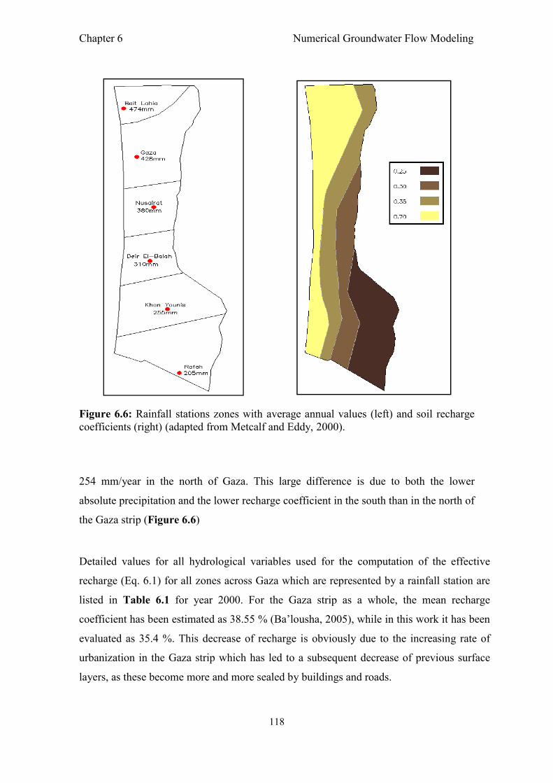
Chapter 6 Numerical Groundwater Flow Modeling
118
Figure 6.6: Rainfall stations zones with average annual values (left) and soil recharge coefficients (right) (adapted from Metcalf and Eddy, 2000).
254 mm/year in the north of Gaza. This large difference is due to both the lower
absolute precipitation and the lower recharge coefficient in the south than in the north of
the Gaza strip (Figure 6.6)
Detailed values for all hydrological variables used for the computation of the effective
recharge (Eq. 6.1) for all zones across Gaza which are represented by a rainfall station are
listed in Table 6.1 for year 2000. For the Gaza strip as a whole, the mean recharge
coefficient has been estimated as 38.55 % (Ba’lousha, 2005), while in this work it has been
evaluated as 35.4 %. This decrease of recharge is obviously due to the increasing rate of
urbanization in the Gaza strip which has led to a subsequent decrease of previous surface
layers, as these become more and more sealed by buildings and roads.

Chapter 6 Numerical Groundwater Flow Modeling
119
Table 6.1: Zonal values for various hydrological variables for year 2000 used for the estimation of recharge.
Station
Soil type Cat. Area (km2)
Average annual rainfall (mm/y)
Average annual ET
(mm/y)
Net average
annual rainfall
(mm/y)
Recharge coefficient
%
Average annual
recharge (m3/y)*103
Average annual recharge (mm/y)
(1) (2) (3) (4) (5) (6)= (4-5) (7) (8)=(6*7*3) (9)= (6*7)
Beit-Hanoun
Dark/ reddish brown
29.00 418 70 348 0.35 3532 121.8
Beit-Lahia Sandy regosols
14.25 433 70 363 0.7 3621 254.1
Jabalia Sandy regosols
15.50 421 70 351 0.25 3808 245.7
Shati Sandy regosols
2.25 392 70 322 0.2 507 152.1
Gaza-City Sandy regosols
13.00 370 70 300 0.25 2730 210
Tuffah Dark/ reddish brown
23.25 425 70 355 0.35 2889 124.25
Gaza-South Dark/ reddish brown
35.00 394 70 324 0.35 3969 113.4
Nusseirat Sandy loess soil
29.50 354 70 284 0.3 2513 85.2
D-Balah Sandy loess soil
38.50 324 70 254 0.3 2934 76.2
Khanyunis Sandy regosols
83.50 290 70 220 0.7 12859 154
Khuzaa Sandy loess soil
42.50 245 70 175 0.25 2231 52.5
Rafah Sandy loess soil
38.75 236 70 166 0.25 1929 50
Total
365.0 358 70 289
35.4 43523 142
6.3.2.2. Lateral inflow
Under natural conditions, the groundwater flow in the Gaza strip is generally directed
from east to west. Lateral subsurface inflow into the Gaza coastal aquifer arises from
the Israeli eastern side of the model domain, which is congruent with the political
border between Gaza and Israel (see Figure 6.10), and it is represented in the model by
placing a series of injection wells with some specified recharge rates along this

Chapter 6 Numerical Groundwater Flow Modeling
120
boundary. These wells are specified with top and bottom screen depths consistent with
the bottom and upper elevations of the aquifer. The amount of inflow varies for each
year, depending on the head variation, as computed by Darcy’s law at the eastern border
of the Gaza strip. Metcalf and Eddy (2000) state the amount of lateral inflow to be
within the range of 15-30 M m3/y. Similar to the recharge, the exact amount of this
lateral inflow has to be determined during the calibration of the groundwater flow
model. Thus, for year 2000, the amount of lateral flow turns out to be 20 M m3.
6.3.2.3. Return Flows
6.3.2.3.1. Irrigation return flow
According to the Gaza Department of Agriculture (GDA), the total amount of the
annual agricultural groundwater abstraction ranges between 80 and 100 M m3/year,
while the amount of irrigation return flow has been estimated as 15-30% of the total
irrigation consumption. Melloul and Collin (1994) estimated the amount of irrigation
returns flow to be about 20% of the total pumping amount (Ba’lousha, 2005). Knowing
that the agricultural groundwater consumption for year 2000 is 85 M m3/year, this
means that 17 M m3/year of return flow infiltrates back into the Gaza coastal aquifer.
6.3.2.3.2. Water system leakage return flow
Another source of return flow into the aquifer is leakage from the rather poorly
maintained water distribution system in the Gaza strip. Accurate monthly pumping
records for municipal wells abstraction indicate that for year 2000, the total domestic
water demand is about 56 M m3 (PWA, 2010a). This amount includes the aquifer
abstraction and Mekorot water, where the latter is being bought from Israel based on the
OSLO “I” - agreement of 1993.
The overall supplied quantity of Mekorot water for year 2010 was 4.88 M m3 and was
distributed to different municipal areas, particularly in the middle and eastern areas of
Gaza.

Chapter 6
Figure 6.7: Municipal water production and consumption for time period
Figure 6.7 depicts the yearly water wells production and consumption
consumed in Gaza comes from the numerous municipal wells which are spread across
98% of the Gaza region, in addition to the agricultural wells. One may note from this
figure that both the production and consumption demands have
increasing over time. Meanwhile,
which is indicative of the large degree of water leakage from the drinking water system
which amount to 16.8 M m
corresponding to a whopping 30
by year 2010 (PWA, 2010a
6.3.2.3.3. Wastewater return flow
The amount of wastewater
Ba’lousha (2005) (cited in the
wastewater return flow in 1998
return flow for year 2000 is
system network, septic tanks, infiltration at the Wadi Gaza area, and infiltration from the
B/Lahia wastewater treatment plant, in portions as
• Leakage from sewer system network
0
10
20
30
40
50
60
70
80
90
100
2000 2001
Wat
er P
rod
./C
on
s.(M
CM
)
Total well Production
Total water consumption
Chapter 6 Numerical Groundwater Flow Modeling
121
Municipal water production and consumption for time period
depicts the yearly water wells production and consumption. Most
consumed in Gaza comes from the numerous municipal wells which are spread across
98% of the Gaza region, in addition to the agricultural wells. One may note from this
both the production and consumption demands have been
Meanwhile, there is a consistent discrepancy between the two,
which is indicative of the large degree of water leakage from the drinking water system
16.8 M m3 for year 2000 and which has been increas
corresponding to a whopping 30-40 % of the total municipal drinking water production
2010a).
Wastewater return flow
wastewater leakage in the Gaza strip is also significant. According to
ed in the study done by LEKA, 2000), the estimated amount of
wastewater return flow in 1998 was 12 M m3. In this study, the amoun
is estimated at 8.5 M m3 and it includes leakage from the sewer
system network, septic tanks, infiltration at the Wadi Gaza area, and infiltration from the
ahia wastewater treatment plant, in portions as listed below:
• Leakage from sewer system network: 2.5 M m3 per year.
2001 2002 2003 2004 2005 2006 2007 2008 2009
Year
Total well Production
Total water consumption
Numerical Groundwater Flow Modeling
Municipal water production and consumption for time period 2000-2010.
. Most of the water
consumed in Gaza comes from the numerous municipal wells which are spread across
98% of the Gaza region, in addition to the agricultural wells. One may note from this
been continuously
there is a consistent discrepancy between the two,
which is indicative of the large degree of water leakage from the drinking water system,
increasing with time,
municipal drinking water production
significant. According to
, the estimated amount of total
the amount of wastewater
leakage from the sewer
system network, septic tanks, infiltration at the Wadi Gaza area, and infiltration from the
2009 2010

Chapter 6 Numerical Groundwater Flow Modeling
122
• Leakage from septic tanks or cesspits: 2 M m3 per year.
• Infiltration at Wadi Gaza area: 2 M m3 per year.
• Infiltration from B/Lahia WWTP: 2 M m3 per year.
6.3.2.4. Wells abstraction
Abstraction of groundwater by pumping wells is the main internal hydrologic stresses
acting on the Gaza aquifer system. More than 4000 water wells have been dug across
the Gaza strip over the recent decades, to meet both the domestic and agriculture
demand (Figure 6.8).
Figure 6.9 shows the total yearly amount of groundwater abstraction from all of these
wells for the 2000-2010 time period. One may notice that the abstraction has been
increasing steadily over the last decade from 136 M m3 in 2000 to 174 M m3 in 2010
(PWA, 2010a). As this increasing demand is not balanced anymore by natural
replenishment from precipitation, the extreme overexploitation of the Gaza aquifer has
gone from bad to worse.
6.3.3. Boundary conditions of the model
The 3D conceptual model box of the Gaza aquifer is enclosed by boundary surfaces, on
which appropriate boundary conditions must be imposed, before the numerical solution
of the 3D groundwater flow equation can be endeavored. There are two types of
boundaries in the conceptual model: Constant head (Dirichlet) boundaries and flux/no-
flow (Neumann) boundaries. The two panels of Figure 6.10 illustrate the boundary
conditions imposed on the Gaza groundwater flow model and they can be enumerated
as follows
1) Dirichlet boundary conditions
A Dirichlet boundary condition of constant head h = h0 = 0 m ASL is assigned at the
western boundary for each layer of the model, which corresponds to the Mediterranean
sea coastline.

Chapter 6 Numerical Groundwater Flow Modeling
123
Figure 6.8: Map of 4000 municipal and agricultural water wells distributed across Gaza.
Figure 6.9: Total yearly wells abstraction from the Gaza aquifer between 2000-2010.
80000 85000 90000 95000 100000 105000
75000
80000
85000
90000
95000
100000
105000
110000
A-180
A-185C-127
C-128
C-76
C-79AD-2
D-601
D-67
D-68
D-69
D-70
D-71
D-72
D-73
D-74
Debri
E-1
E-142
E-154
E-156E-157
E-4
E-6 E-61
E-90
G-16
G-30
G-49
J-146
J-32
K-19
K-20K-21
L-127
L-159L-159A
L-176
L-179A
L-182
L-184
L-187
L-189
L-41
L-43
L-87
L-I286
Mog
Mog1
Msalam
Mun.
New
P-124
P-138
P-139
P-144
P-15
P-153
P-52
priv.
Q-40A
Q-68
R-112R-113
R-162BA
R-162CA
R-162D
R-162EA
R-162G
R-162HR-162HA
R-162LR-162LB
R-254
R-25AR-25BR-25CR-25D
R-265
R-74
R-75
S-37
S-69
S-72
N1
N10
N11
N14
N15
N16
N17N18
N19
N2
N20N21
N22
N23
N24N25
N3
N4 N5
N6
N7
N8
N9
Y1Y2
Y3
Y4
Y5
T26
T27
T28
T30
T31T32
T33T34
T35
T38
T39
T4
T40
T41
T6
T8
T9
kh137
T12
T13
T14T15
T16T17
T18 T19
T2
T20T21
T22T23
T24
T25
M1
M10
M2A
M2B
M3
M4 M5
M6
M7
M8
M9
MI1
MI2
MI3
L11
L110L111
L112L113
L114
L115
L116L117
L118
L119
L120L121
L122L123
L124
L126
L128
L129
L13
L130
L131
L132
L133
L134L135
L136
L137L138
L139
L14
L140
L141
L142
L143
L144
L145
L15
L150
L151L153
L154L155
L156
L157
L16
L160L161
L162
L163
L164
L165
L166
L167
L17
L170
L172
L173
L174
L177
L178
L179B
L18
L19L20L21L22
L24L25
L26L27
L28 L29L30
L31L32
L33
L34
L35
L36
L37
L38
L39
L4
L40
L42
L45
L46
L47L48L49
L5
L66
L67
L68L69
L7
L70
L71L72
kh1
kh5
kh6
kh31
kh32
kh44
kh49
kh53
kh54
kh55
kh63
kh74
kh80
kh90
kh114
kh116kh127
kh128
kh145
kh163
kh172
kh184
kh191
kh233
kh234
kh245
kh286
Raf11
Raf14
Raf25Raf39
Raf46
Raf51
Raf64
Raf77
Raf80
P51
P53
P54
P55
P56P57
P58
P59
P6
P60
P61
P62
P63
P64P65
P66
P67P69
P70
P71
P72
P73P74
P75
P76P77
P78
P79P80
P81
P82
P83
P84P85
P86AP86B
P86C
P88
P89P90
P91
P92
P93P94
P96
P97
P98P99
P120
P121P122
P123
P125
P126
P127
P13
P130
P131
P132
P133
P135
P136
P137
P140
P141
P142
P145
P147
A1
A10
A100
A101A102
A103
A104
A104A
A105
A106
A107
A108A109
A11
A110
A111
A113A114
A115
A116
A117
A118
A119
A12
A120
A121
A122
A123
A124
A125
A126
A127 A128A129
A13
A130
A131A132
A133
A134
A136
A137
A138
A139
A14
A140
A141A142
A143
A144
A145
A146
A147
A148A149
A15
A150
A151
A152
A153
A154
A156
A157
A158
A159
A16
A160
A161
A162
A163
A165
A166
A167
A168
A169
A17
A170
A171
A172
A173
A174
A175
A176
A177
A178
A179
A18
A181
A182
A183
A184A186
A187
A188
A189
A19
A190
A191
A192
A193
A194
A20A21
A22A23
A24A25
A26A27
A28
A29
A2A
A2B
A2C
A2D
A3
A30A31
A32A33
A34
A35
A37
A38
A39
A4
A40
A41
A42
A43
A44
A45
A46
A47A48
A49
A5
A50A51A52
A53
A54
A55 A56A57
A58
A59
A6
A60
A61
A62A63
A64
A65
A66
A67A68A681
A69
A7
A70
A71
A72A73
A74
A75
A76
A77
A78
A79
A8
A80
A81A82
A83
A84
A86A87
A88A89
A9
A90A91
A92A94A95A96
A97A98
A99
C1
C10
C100C101
C102
C103C104
C105
C106
C107C108C109
C110C111
C112
C113
C114
C115
C116
C117
C118
C119 C11A
C11B
C120
C121 C122
C123
C124
C125
C126
C129
C12A
C12BC12C
C12D
C13
C130
C14
C15A
C15B
C16A
C16B
C17A C17BC17CC18
C2
C20
C21C22
C23C24 C25
C26
C27
C28
C29
C30
C31C32C33
C34
C35
C36
C37
C38C39
C3A C3B
C3C
C3DC3E
C40
C42
C43
C44C45
C46
C47A
C47B
C48
C49
C4A
C4B
C5
C50
C51
C52C53
C54
C55AC55B
C56AC56B
C57
C58C59
C6
C60
C62
C63
C64C65
C66
C67C68
C69
C7
C70C71
C72
C73C74
C75
C77
C78
C79
C8
C80C81C82
C83C84
C85C86
C87
C88C89
C9
C90C91 C92
C93C94
C95C96
C97
C98C99
C-I-1
C-I-10
C-I-11
C-I-12
C-I-13C-I-14
C-I-15
C-I-16
C-I-17
C-I-2
C-I-3C-I-4
C-I-6
C-I-7C-I-8
C-I-9
Q1
Q2
Q23Q24Q25
Q26Q27
Q28
Q29
Q14Q15
Q16
Q17Q18
Q20Q21
Q22
Q19Q10
Q11
Q12
Q13
B1
B10
B11B12B13
B14B15
B16B17
B18
B19
B2
B20
B21
B22
B23
B24
B25
B3B4
B5
B6
B7 B8B9
D16D17
D18
D20D21D22
D23
D24D25
D26
D27
D28
D29
D3
D30D31
D32
D33D34 D35D36
D37D38
D39
D4
D40
D41 D42D43D44D45
D46
D47D48
D49
D5
D50D51
D52D53
D54D55
D56
D57
D58
D59
D6
D61
D62
D63
D64
D65
D66D7
D8
D9
E110E111E112
E113E114A
E115E116
E117E118
E119
E11A
E11BE11C
E12
E120
E121
E122
E123
E124
E126
E128E129
E13
E130
E131
E132
E133
E134E135
E136
E137
E138
E14
E143
E144
E145E146
E147E148
E149
E15
E150
E152
E153
E155E158
E159
E16
E160
E17
E18E19
E21
E22
E23E24AE24B
E25
E26
E28
E3
E30E31
E32
E33E33AE34
E35
E36E37
E38E39
E40E41E42
E43
E44
E45
E46 E48
E49 E5E50
E51E52
E53E54
E55E56E57
E58E59
E6
E60
E62
E63 E64E65
E66
E67E68
E68A
E69
E7
E70E71
E73 E74
E75E76E77
E78E79E80
E81E82
E84
E85E86
E87E88E89
E91
E93E94
E95E96E97
E98E99
F121F122
F122'
F123F124
F125
F126
F127
F128
F129
F13
F130A
F130B
F131F132F133
F134F135
F136
F137
F137n
F138F139
F14
F140
F141
F142
F143
F144
F145
F146
F147
F148
F149
F15
F150
F151
F152
F153F154F155
F156 F157
F158
F159
F16
F160
F161
F162
F163
F164
F165
F166
F167
F168F169
F17
F170
F171
F172
F173
F174
F176F177
F178F179
F18
F180
F181
F182
F183
F184
F185
F186
F188
F189
F19
F191
F2
F20F21
F23A
F23B
F24F25F26
F28F29
F30A
F30B
F31F32
F33
F34
F35
F36
F38
F39
F4
F40
F41F42
F43
F44
F45
F46
F47
F48F49
F5
F50F51
F52F53
F54F55
F56
F57F58
F59F60
F61
F62F63F64
F65
F66
F67
F68AF68B
F69A
F69B
F7
F70
F71F72
F73F73A
F74
F76
F76A
F77F78 F79
F8
F80F81F82F83
F84
F85
F86F87
F89
F9
F90
F91
F92
F93F94
F95 F96
F97
F98F99
G27
G28
G3
G31
G32
G33
G34
G35
G36G37
G38G39
G40
G41
G42
G43
G44
G45
G4AG4B
G5
G50
G501
G502
G503
G504
G505AG505B
G507
G508
G509
G510
G511
G512
G513
G6
G7G8G9
Gaz1
Gaz100
Gaz101
Gaz102Gaz103
Gaz104
Gaz105
Gaz106
Gaz107
Gaz108
Gaz109
Gaz11
Gaz110
Gaz111
Gaz113
Gaz114
Gaz115
Gaz116
Gaz117
Gaz118
Gaz119
Gaz12
Gaz120
Gaz121
Gaz122
Gaz123
Gaz124
Gaz125
Gaz126
Gaz127
Gaz13
Gaz14
Gaz15
Gaz16
Gaz17
Gaz18
Gaz2
Gaz20
Gaz21
Gaz22
Gaz23
Gaz24
Gaz25
Gaz27
Gaz28
Gaz29
Gaz3
Gaz30
Gaz31Gaz32
Gaz33
Gaz34Gaz35
Gaz36
Gaz37
Gaz38
Gaz39Gaz4
Gaz40
Gaz41
Gaz42
Gaz43
Gaz44
Gaz45
Gaz46
Gaz47
Gaz48
Gaz49
Gaz5
Gaz50
Gaz51
Gaz52
Gaz53
Gaz54
Gaz55
Gaz56
Gaz57
Gaz58
Gaz59
Gaz6
Gaz60
Gaz61
Gaz63
Gaz64
Gaz65
Gaz66
Gaz67
Gaz68
Gaz69
Gaz7
Gaz70
Gaz71
Gaz72
Gaz74
Gaz75
Gaz76
Gaz77
Gaz78
Gaz8
Gaz80
Gaz81
Gaz82
Gaz83
Gaz84
Gaz85
Gaz86
Gaz87
Gaz88
Gaz89
Gaz90
Gaz91
Gaz92
Gaz93
Gaz94
Gaz95
Gaz96
Gaz97
Gaz98
Gaz99
H10
H1001
H1002H1003
H1005H1006H1007
H1008
H1010
H11H12
H13H14
H15H16H18
H19
H2
H20
H21
H23
H24
H25
H26
H27H28
H29
H3
H30
H32
H33
H34 H35
H36H37H38
H39
H4
H40
H41
H42
H43
H44H45
H47
H49
H5
H50
H501 H502H503
H504
H505H506
H507
H508H509
H51
H510
H511 H512
H513
H514H515
H516
H517
H518H519
H52
H520H521
H522
H524
H525
H527
H528
H529AH53
H531H532
H533
H534
H535
H537
H538
H539
H54
H540H543
H57
H58H59
H6'
H60
H61
H62H63
H64H65
H67
H69
H7
H70
H72H73
H74
H77
H78
H8
H80
H81n
H82
H83
H84H85
H86
H87
H88
H9
H90
H91
H92
H93
J1
J10
J 100
J1001
J1002
J101
J102
J103J104 J106
J107
J108
J109
J11
J110
J111
J112
J114
J115
J116J117
J118J119
J12
J120J121
J122
J124
J125
J126'
J127
J128
J13
J130
J131
J133
J134
J135
J136
J137 J138
J139
J14
J141
J142
J143
J144
J145
J148
J149
J15
J151
J153
J154
J16
J17J18
J19
J2
J20
J21
J22J23
J24J25
J27
J28
J29
J3
J30J36
J37
J4
J43
J44
J45J46
J47J48
J49J50
J501
J502J504
J507
J509
J51J52
J54A
J54B
J54CJ54DJ54E
J55J56J57
J58
J59
J6
J60
J61J62
J63J64J66
J67
J68
J7
J70J71
J72
J74 J75
J76
J77
J8
J80J83
J85
J86J87J88
J89
J90J91
J92J93
J94
J95J96J97
J98
J99
K1
K10
K11
K12
K13
K14
K15K16
K17
K2K3
K4
K5
K6
K7
K8
K9
kh10
kh100
kh101kh102
kh103
kh104
kh105kh106
kh107
kh108
kh109
kh11
kh110kh111
kh112
kh113
kh115
kh117
kh118
kh119
kh12
kh120
k h121
kh122kh123
kh124
kh125
kh126
kh129
kh131
kh132 kh133
kh134
kh136
kh138kh139
kh14
kh140
kh141
kh143
kh144
kh146
kh147
kh148
kh149
kh15
kh150
kh151kh152
kh153
kh154
kh155
kh156
kh157
kh158
kh159
kh16
kh160
kh161
kh162
kh164
kh165
kh166
kh167
kh168
kh169
kh17
kh170
kh171
kh173
kh174
kh175
kh176
kh177
kh178
kh179
kh18
kh180
kh181kh182
kh183
kh186
kh187
kh188
kh189
kh19
kh192
kh193
kh194kh195kh196
kh197
kh198
kh199
kh2
kh200
kh201
kh202
kh203
kh204
kh205
kh206
kh207
kh208 kh209
kh21
kh210
kh211
kh212
kh213
kh214kh215kh216
kh217
kh218
kh219
kh22
kh220
kh221
kh222
kh223
kh224
kh225
kh226
kh227
kh228
kh229
kh23
kh230kh231
kh232
kh235
kh236
kh237
kh238
kh239
kh24
kh240
kh242
kh243
kh244
kh247
kh248kh249
kh25
kh250
kh251
kh252
kh253kh254
kh255
kh256
kh257
kh258
kh259kh26
kh260
kh261
kh262
kh263
k h264
kh265
kh266
kh267
kh268
kh269
kh27
kh270
kh271
k h272
kh273
kh274
kh275
kh276
kh277
kh278
kh279
kh28
kh280
kh281
kh282
kh283
kh284
kh285
kh287
k h288
kh289
kh29
kh290
kh291
kh292
kh293
kh294
kh295
kh296kh297kh298
kh3
kh30
Kh300
Kh301
Kh302
Kh303
Kh305
Kh306
Kh307
Kh308
Kh309
kh310
kh311
kh312
kh313
kh314
kh315
kh316
kh317
kh318
kh33
kh34
kh35
kh36
kh37
kh38
kh39
kh4
kh40
kh41
kh42
kh43
kh45
kh46
kh47
kh48
kh50
kh51
kh52
kh56
kh57
kh58kh59
kh60
kh61
kh62
kh64
kh65
kh66
kh67
kh68
kh69
kh7
kh70
kh71kh72
k h76
kh77
kh79
kh8
kh81
kh82kh83
kh84
kh85
kh86
kh87
kh88
kh89
kh9kh91
kh92
kh93
kh94
kh95
kh96
kh97
kh98
kh99
KI1
KI2
KI3
L10
L1003
L1007
L1008
L101
L1011
L1012
L1014
L1015
l1016L1017
L1019
L102L103
L104
L105
L106
L107
L108
L109
L181
L1A
L1Bn
L1Bo
L2
L50
L501
L503
L504
L505L506L507
L508L509
L51
L510
L512L513
L514 L515L516
L517L519
L52L52'
L520L521
L522L523
L524
L526
L527
L528
L529
L53
L532
L534
L536L537
L539L540L541
L542L543
L545 L546
L547
L548
L55
L550L551L552L553L554
L555L556L557
L559
L56
L560
L562L563L564
L566
L569
L57
L570
L572L573L574L576
L577L578L579
L58
L580
L581L582L583L587
L59
L591L592L593
L594
L595BL595A
L596L597L598
L6
L60
L602
L603
L605L607
L61
L612
L613
L615
L616L617
L618L619
L62
L621
L622
L624
L625nL625o
L626
L627
L628
L63
L630
L632
L635
L637L638'
L64
L641
L643L644
L647
L648
L65
L650
L73A
L73B
L73C
L74
L76
L77
L78
L8
L80
L81
L83
L84
L85
L86n
L88
L89
L9
L90
L91
L92
L93L94
L95 L96
Mid1
Mid10Mid100
Mid101
Mid103
Mid104 Mid105
Mid106
Mid107
Mid108
Mid109
Mid11
Mid110
Mid111
Mid112
Mid113
Mid114
Mid115
Mid116
Mid117Mid118
Mid119
Mid120
Mid121
Mid122
Mid123
Mid124
Mid125
Mid126
Mid127
Mid128
Mid129
Mid13
Mid130
Mid131
Mid132
Mid133
Mid134
Mid135
Mid136
Mid137
Mid138
Mid139
Mid14
Mid140
Mid141
Mid142
Mid143
Mid144
Mid145
Mid146
Mid147
Mid148
Mid149
Mid150
Mid151
Mid152
Mid153
Mid154
Mid155
Mid156
Mid157
Mid159
Mid16
Mid160
Mid161
Mid162
Mid164Mid165
Mid166
Mid167Mid168
Mid169
Mid17
Mid170
Mid171
Mid172
Mid173
Mid174
Mid175
Mid176
Mid177
Mid178
Mid179
Mid18
Mid19
Mid2
Mid20
Mid21
Mid22
Mid23
Mid24
Mid25
Mid26
Mid27
Mid29
Mid3
Mid30
Mid31
Mid32
Mid33
Mid34Mid35
Mid36
Mid37
Mid38
Mid4
Mid40Mid41
Mid42
Mid43
Mid44Mid45
Mid46
Mid47
Mid48
Mid49
Mid5
Mid50 Mid51
Mid52
Mid53
Mid54Mid55
Mid56
Mid57
Mid58
Mid59
Mid6
Mid60
Mid61
Mid62
Mid63
Mid64
Mid65
Mid66
Mid67
Mid68
Mid69
Mid7
Mid70
Mid71
Mid72
Mid73
Mid74
Mid75Mid76
Mid77
Mid78
Mid79
Mid8
Mid80
Mid81
Mid82
Mid83Mid84
Mid85
Mid86
Mid87
Mid88
Mid89
Mid9
Mid90
Mid91
Mid92
Mid93
Mid94
Mid95
Mid96
Mid97
Mid98
Mid99
MSALM
NI5
Nor1
Nor10
Nor11
Nor12
Nor13
Nor14
Nor16
Nor17
Nor18Nor19
Nor2
Nor20
Nor21
Nor22
Nor23
Nor24
Nor25
Nor26
Nor27
Nor28
Nor29
Nor3
Nor30
Nor31
Nor32
Nor33
Nor34Nor35
Nor36
Nor37
Nor38Nor 39
Nor4
Nor40
Nor6
Nor7
Nor8
Nor9
P1008
P101
P1012P1015
P1017 P1018
P1019
P102
P1023P1024
P1025
P1026
P103
P1032
P104
P105
P106P107
P108
P109P110P111
P112
P113
P114P116
P117
P118
P119
P12
P16BP17
P18
P2
P21
P22
P24
P26
P27
P28
P29
P31
P32
P33
P34
P35P36
P37
P38
P39P41
P42
P43P44
P45P46
P47
P48AP48B
P49
P50
P501
P506
Q3
Q30
Q31Q32
Q33Q34
Q35Q36
Q37
Q38Q39
Q4Q40B
Q41
Q42
Q43
Q44Q45
Q46Q47
Q48Q49
Q5
Q50
Q51
Q52
Q53Q54A
Q54B
Q54CQ54D
Q54E
Q54FQ55
Q56
Q57
Q58
Q59
Q60
Q61
Q62Q63
Q64Q65
Q67
Q69
Q7
Q8
Q9
QI224AQI225A
R102
R103
R106
R107
R11
R110R111
R114
R116
R12
R120R121R123R124
R125R126
R127
R128R129
R13
R130
R132
R133
R134
R135
R136
R137
R138
R139
R14
R140R141
R142R143
R144
R146
R147
R15
R150R153
R155
R160
R161
R162A
R162B
R162CR162E
R162F
R162Hn
R162Ln
R16AR16B
R17
R170
R171
R174
R176R177
R178
R179
R18
R183
R184
R185R186
R187R188
R189
R19
R190 R192R193
R194R195
R197R198
R199
R2
R20R2011R202R203
R204R205
R206R207R208
R209
R210
R211
R212
R213
R214
R215
R216
R217 R218
R219
R22
R221R222
R223
R223n
R224
R225
R227R228
R23
R230
R231
R232
R233
R234
R235
R236R237
R238
R24
R241
R242
R243
R244
R245
R246
R247
R249
R250
R251
R252
R253
R255
R256
R257
R258
R259
R260
R261
R262
R263
R264
R26AR27
R271
R272A
R273
R274
R275
R277
R28R29
R3
R30R31
R32R33
R34R35
R36R37
R38
R4
R40R41
R42
R43R44
R46
R47
R48
R49
R5
R50R51
R52
R53
R54
R56R57R58R59
R6
R60
R62R63
R65
R66AR66B
R67
R68
R69
R7
R72
R76
R79
R81
R82R83
R84
R85
R86R87
R88
R8A
R8B
R9
R90
R91R92
R93
R94
R96
R98R99
Raf1
Raf10
Raf12
Raf13
Raf15
Raf16
Raf17
Raf18
Raf19
Raf2
Raf20
Raf21
Raf22
Raf23
Raf24
Raf26
Raf27
Raf28
Raf29
Raf3
Raf30
Raf31
Raf33
Raf34
Raf35
Raf36
Raf37
Raf38
Raf4Raf40
Raf41
Raf42
Raf43
Raf44
Raf45
Raf47
Raf48
Raf49
Raf5
Raf50
Raf52
Raf53
Raf54
Raf55
Raf56
Raf57
Raf58
Raf59
Raf6
Raf60
Raf61
Raf62
Raf63
Raf65
Raf66
Raf67
Raf68
Raf69 Raf7
Raf70
Raf71
Raf72
Raf73
Raf74
Raf75
Raf76
Raf78Raf79Raf8
Raf9
S52
S53
S54
S55
S56S57
S58
S59
S6
S60
S61
S62
S63
S64
S65
S66
S68
S69
S7
S70
S71
S8
S9
24
27
29
25A
26B
D10
D11
D12
D13
D14D15
E10
E100E101E102
E103E104
E105
E106
E107
E108
E83
Nor5
Zimo
R1
R10
2A
36B
6A
8A
F100
F101F102
F103F104A F104B
F104C
F105F106
F107
F108
F109
F110
F111
F112F113
F114
F115
F116
F117
F118F119
F120
F120A
R101
Well3
Well4G24A
G24B
G24C
S1
S2
S4
S10
23
22A
3A
cost1
cost2
cost3
DIBRI
F1
G1
G10 G11
G12
G13
G14
G17
G18
G19
G2
G20G21
G22G23
G25
G26
G49
J54En
S45n
S12
S13S14
S15
S16
S17
S18S19
S21
S22
S23
S24
S25
S26
S27
S28
S29S30
S31S32
S33S34
S35
S36S38
S39S40
S41
S42
S44
S45
S46
S47
S48
S49
S50
S51
S72
F11F12
F10
T43
T1
T29T3
T36
T37A
T42
T44
T7
coast4
12
18
21
37B
coast5
EV02
K19
L96n
L127
L159L159A
L171
L176
L179A
L182
10A
7
13
P1027
P10
P100
P52
P1001
P1005
A-I-1
A-I-10A-I-11
A-I-12
A-I-13
A-I-14
A-I-15
A-I-16
A-I-17
A-I-19
A-I-20
A-I-21
A-I-22
A-I-23
A-I-24A-I-25
A-I-26
A-I-27A-I-28
A-I-29
A-I-3
A-I-30
A-I-31
A-I-32
A-I-33
A-I-34
A-I-35
A-I-36A-I-37
A-I-38
A-I-39
A-I-4
A-I-40A-I-41
A-I-42
A-I-43
A-I-44
A-I-45
A-I-46 A-I-47
A-I-48
A-I-49
A-I-5
A-I-50
A-I-6A-I-7A-I-8A-I-9
B-I-1
B-I-2 B-I-3
E-I- 10E-I-11
E-I-13
E-I-14E-I-15E-I-16
E-I-22
E-I-23
E-I-24E-I-25
E-I- 6
E-I-8E-I-9
R-I-89
R-I-90
F-I-1
F-I-10
F-I-100
F-I-101
F-I-102
F-I-103F-I-104F-I-105
F-I-106F-I-107
F-I-109
F-I-11
F-I-110
F-I-111
F-I-112
F-I-113
F-I-114
F-I-115
F-I-116
F-I-118
F-I-119
F-I- 12
F-I-120F-I-121
F-I-122
F-I-123
F-I-124
F-I-125
F-I-126
F-I-127
F-I-128
F-I-129
F-I-13
F-I-130
F-I-14
F-I-15
F- I-16
F-I-17
F-I-18
F-I-19
F-I-2
F-I-20
F-I-21
F-I-22F-I-23
F-I-25
F-I-26F-I-27F-I-28
F-I-29
F-I-3
F-I-30F-I-31
F-I-32
F-I-33F-I-34F-I-35
F-I-36
F-I-37
F-I-38
F-I-39
F-I-4
F-I-40
F-I-41
F-I-42
F-I-43
F-I-44
F-I-47
F-I-48F-I-49
F-I-5
F-I-50
F-I-51
F-I-52
F-I-53
F-I-54
F-I-55
F-I-56F-I-57
F-I-58F-I-59
F-I-6F-I-60F-I-61F-I-62
F-I-63
F-I-64F-I-65
F-I-66F-I-67
F-I-68F-I-69F-I-7
F-I-70
F-I-71
F-I-73F-I-74
F-I-75
F-I-76F-I-78F-I-79
F-I-8F-I- 80
F-I-81
F-I-82F-I-83
F-I-84
F-I- 85
F-I-86F-I-87
F-I-88
F-I-89
F-I-9F-I-90
F-I-91F-I-92F-I-93
F-I-94F-I-95
F-I-96F-I-97
F-I-98F-I-99
R-I-1
R-I-10
R-I-11R-I-12
R-I-13R-I-14
R-I-15
R-I-16R-I-17
R-I-18
R-I-19
R-I-2
R-I-20
R-I- 21
R-I-22
R-I-23
R-I-24
R-I-25
R-I-26
R-I-27
R-I-28R-I-29
R-I-3
R-I-30
R-I-31
R-I-32
R-I-34R-I-35
R-I-36R-I-37
R-I-38R-I-39
R-I-4
R-I-40
R-I-41R-I-42
R-I-43
R-I-45
R-I-46
R-I-47
R-I-48
R-I- 5
R-I-50
R-I-51
R-I-52
R-I-53
R-I-54
R-I-55
R-I-56
R-I-57
R-I-58R-I-59
R-I-6
R-I-60R-I-61R-I-62
R-I-63
R-I-64R-I-65
R-I-66
R-I-68
R-I-69
R-I-7
R-I-70
R-I-71R-I-72R-I-73
R-I-74
R-I-75
R-I-76
R-I-77
R-I-78
R-I-79
R-I-80R-I-81R-I-82
R-I-83
R-I-84
R-I-85R-I-86
R-I-87
R-I-9
R-I-91
R-I-92
R-I-93
E-I-18
E-I-19E-I-20E-I-21
E-I-17
E-I-5
G-I-1G-I-2
G-I-3
G-I-4
G-I-47
G-I-10G-I-11
G-I-12G-I-13
G-I-14G-I-15G-I-16G-I-17
G-I-18G-I-19
G-I-20
G-I-21G-I-22
G-I-23G-I-24
G-I-25G-I-26
G-I-27
G-I-28
G-I-29G-I-30G-I-31G-I-32
G-I-33G-I-34
G-I-35
G-I-36
G-I-37G- I-38
G-I-39
G-I-40
G-I-41
G-I-42
G-I-44G-I-45
G-I-46
G-I-48
G-I-49
G-I-5G-I-6G-I-7
G-I-8G-I-9
H-I-1
H-I-10
H-I-11
H-I-12
H-I-13H-I-14
H-I-15
H-I-16
H-I-17
H-I-19
H-I-2H-I-20H-I-21
H-I-23H-I-24
H-I-25
H-I-26H-I-27
H-I-28
H-I-29
H-I-3
H-I-30
H-I-31
H-I-32
H-I-33
H-I- 34H-I-35
H-I-36
H-I-37H-I-38
H-I-39
H-I-4
H-I-40
H-I-41
H-I-42
H-I-43H-I-44H-I-45
H-I-46
H-I-47
H-I- 48
H-I-49
H-I-5
H-I- 50
H-I-51
H-I-52
H-I-53
H-I-54H-I- 55
H-I-56
H-I-6H-I-7
H-I-8H-I-9
J-I-1
J-I-10
J-I-11J-I-12
J-I-13J-I-14
J-I-15J-I-16J-I-17J- I-18
J-I-19
J-I-2J-I-20J-I-21
J-I-22
J-I-23
J-I-24
J-I-25
J-I-26J-I-27
J-I-28
J-I-29
J-I- 3
J-I-30J-I- 31
J-I-34J-I-35
J-I-36 J- I-37
J-I-38
J-I-39
J-I-4
J-I-40
J -I-41J-I-42J-I-43J-I-44
J-I-46
J-I-47
J-I- 48J-I-49
J-I-5
J-I-50J-I-51
J-I-52
J-I-53 J-I-54
J-I-55
J-I-56
J-I-57
J-I-58J-I-59
J-I-6
J-I-60
J-I-61
J-I- 62
J -I-63
J-I-64
J-I-65
J-I-66
J-I-67
J-I-68
J-I-69
J-I-7
J-I-70
J-I-71
J-I-72
J-I-73
J-I-74
J-I-75
J-I-76
J-I-77
J-I-78
J-I-79
J-I-8
J-I-80
J-I-81
J-I-82
J-I-83
J- I-85J-I-86
J-I-87
J-I-88
J-I-9
J- I-90
S-I-1
S-I-10
S-I-11
S-I-12
S-I-13 S-I-14S-I-15S-I-17
S-I-18S-I-19
S-I-2
S-I-20
S-I-21
S-I-22
S-I-23
S-I-24
S-I-26
S-I-27
S-I-28
S-I-29
S-I-3
S-I-30
S-I-31
S-I-32
S-I-33
S-I-34
S-I-36
S-I-37
S-I-38
S-I-39
S-I-4
S-I-40
S-I-41
S-I-5S-I-6
S-I-7S-I-8 S-I-9
L-I-1
L-I-10
L-I-100
L-I-102L-I-103L-I-104L-I-105
L-I-106L-I-108
L-I-109
L-I-11
L-I-110
L-I-111L-I-112L-I-113L-I-114
L-I-115L-I-116L-I-117L-I-118
L-I-119L-I-120L-I-121L-I-122L-I-123L-I-124
L-I-125
L-I-126L-I-127
L-I-128
L-I-129
L-I-13
L-I-130L-I-131L-I-132
L-I-133 L-I-134L-I-135L-I-136L-I-137
L-I-138L-I-139
L-I-14
L-I-140
L-I-141L-I-142
L-I-143
L-I-144
L-I-146
L-I-147L-I-148
L-I-149
L-I-15
L-I-150L-I-151L-I-152L-I-153L-I-154
L-I-155L-I-156
L-I-157L-I-159
L-I-16
L-I-160
L-I-161
L-I-162L-I-163L-I-164L-I-165L-I-166L-I-167
L-I-168L-I-169
L-I-17
L-I-171
L-I-172
L-I-173L-I-175
L-I-177L-I-178
L-I-179
L-I-18
L-I-180L-I-181
L-I-182
L-I-185
L-I-186L-I-187
L-I-188
L-I-19
L-I-190
L-I-191
L-I-192
L-I-193L-I-194L-I-195L-I-196L-I-197
L-I-198L-I-199
L-I-2
L-I-20
L-I-200L-I-201L-I-202L-I-203L-I-204
L-I-205
L-I-206
L-I-207
L-I-208
L-I-209 L-I-21L-I-210
L-I-211
L-I-212
L-I-213L-I-214L-I-215
L-I-216L-I-217
L-I-218L-I-219
L-I-22
L-I-220L-I-221
L-I-225
L-I-228L-I-229
L-I-230
L-I-231L-I-232
L-I-236
L-I-238
L-I-239
L-I-24
L-I-240L-I-241 L-I-242L-I-243
L-I-244L-I-245
L-I-246
L-I-247
L-I-248
L-I-249L-I-25
L-I-250L-I-251L-I-252L-I-253
L-I-255
L-I-256L-I-257L-I-258L-I-259
L-I-26
L-I-260L-I-261
L-I-262
L-I-263
L-I-264
L-I-265L-I-266L-I-267L-I-268L-I-269
L-I-27
L-I-270L-I-271
L-I-272
L-I-273
L-I-274L-I-275
L-I-276
L-I-277L-I-278L-I-279
L-I-28
L-I-281
L-I-282
L-I-283
L-I-284
L-I-285
L-I-286
L-I-287
L-I-288
L-I-29
L-I-3
L-I-30
L-I-31
L-I-32
L-I-33 L-I-34
L-I-35
L-I-36
L-I-37
L-I-38L-I-39
L-I-4
L-I-40
L-I-41
L-I-42L-I-43
L-I-44
L-I-45
L-I-46
L-I-47L-I-49
L-I-5
L-I-50L-I-51L-I-52L-I-53
L-I-54
L-I-55L-I-56L-I-57
L-I-58
L-I-589
L-I-59
L-I-590
L-I-6
L-I-60
L-I-63L-I-64
L-I-65
L-I-66
L-I-67L-I-68L-I-69
L-I-7
L-I-70L-I-72L-I-73L-I-74
L-I-75L-I-77
L-I-78
L-I-79
L-I-8
L-I-80
L-I-82L-I-83L-I-84L-I-85
L-I-86L-I-88L-I-89
L-I-9
L-I-90L-I-92 L-I-93
L-I-94
L-I-95
L-I-96L-I-97
L-I-98
O-I-4
P-I-111P-I-112P-I-113P-I-114
P-I-115P-I- 117
P-I-120P- I-121
P-I-122
P-I-123
P-I-104
P-I-106
P-I-108P-I-109
P-I-110
P-I-89P-I-95
P-I-96P-I-97P-I-98
P- I-118
P-I-124P-I-93
P-I-1P-I-10
P-I-100P-I-101
P-I-102
P-I-107
P-I-11
P-I-125
P-I-126P-I-128
P-I-131
P-I-14
P-I-15
P-I-16
P-I-17
P-I-18
P-I-2
P-I-20
P-I-21
P-I-23
P-I-24
P-I-25
P-I-26
P-I- 27P-I-28
P-I-29
P-I-3
P-I-30P-I-31
P-I-32P-I-33
P-I-34P-I-35
P-I-36P-I-37
P-I-38
P-I-4
P-I-40
P-I-41P-I-42
P-I-43P- I-44
P-I-45
P-I-46P-I-47
P-I-48
P-I-5
P-I-50
P-I-51
P-I-52
P-I-53P-I-54
P-I-55
P-I-56
P-I-57
P-I-58P-I-59
P-I-6
P-I-60
P-I-61
P-I-63
P-I-64P-I-65
P-I-66
P-I-68P-I-69
P-I-7
P-I-70
P-I-71P-I-72
P-I-74P-I-75
P-I-76
P-I-77P-I-79
P-I- 8
P-I-80P-I-81
P-I-82
P-I-83P- I-84
P-I-85
P-I-86P-I-87P-I-88
P-I-9
P-I-91
P-I-92
P- I-99
D-I-1
D-I-2
D-I-3
R-I-8
P-I-130P-I-90
80000 85000 90000 95000 100000 105000
75000
80000
85000
90000
95000
100000
105000
110000
0 5000 10000 15000
0
20
40
60
80
100
120
140
160
180
200
2000 2001 2002 2003 2004 2005 2006 2007 2008 2009 2010
Ab
str a
ctio
n(M
CM
)
Year
Total Abstraction

Chapter 6 Numerical Groundwater Flow Modeling
124
Figure 6.10: EW- cross section (left) and horizontal map (right) of the model domain with boundary conditions imposed (Sirhan and Koch, 2012b).
2) Neumann boundary conditions
Neumann boundary conditions are used to represent horizontal and vertical influx
boundaries as well as no-flow boundaries, namely
Neumann recharge influx boundaries:
A Neumann flux boundary with the flux representing groundwater recharge by direct
surficial infiltration is specified at the top boundary surface of the model. The averaged
water flux values through the land surface include net infiltration due to rainfall and
return flow from various recharge components, as discussed, namely, irrigation return
flow, leakage from domestic networks and wastewater losses.
A Neumann constant-flux boundary condition of lateral subsurface inflow is also
specified at the eastern boundary which runs along the Gaza-Israel political border.
Practically this is done in the model by placing a series of injection wells with specified
recharge rates (which will be determined during the calibration process) along this
boundary.
Neuman no-
flow boundary
Dirichlet Constant flux BC
Neuman
Constant
flux BC
Neuman influx
boundary

Chapter 6 Numerical Groundwater Flow Modeling
125
Lateral no-flow boundaries:
No-flow boundaries are usually assigned at boundaries which are either physical
limitations of the aquifer or which, by some groundwater flow symmetry, are not
crossed by flow. In the Gaza strip, under natural conditions the flow lines are more or
less directed from east to west, perpendicular to the coastline. For this reason, the
vertical boundaries of the model in the north along the Israel border and in the south
along the Egypt border are assigned as no-flow boundaries.
Per default, a Neumann lateral no-flow boundary is implicitly specified at the bottom
boundary surface of the model, which here corresponds to the top of the Saqiya
impermeable clay layer, with a thickness ranging between 400-1000 m (see Chapter 3).
6.3.4. Initial conditions
For the transient groundwater flow simulations that cover the time period 2001-2010,
initial conditions for the groundwater heads, distributed across the model area, must also
be set. In the present application these are the simulated water levels for year 2000, as
obtained during the steady-state calibration of the model, and they are assigned as initial
condition for the transient simulation.
6.3.5. Hydraulic aquifer parameters
The important hydraulic aquifer parameters assigned to the model in the initial phase of
the calibration process have been obtained from pumping tests, which were carried out
for different municipal wells as a part of the project of CAMP-2000, under the
monitoring of the Palestinian Water Authority (PWA).
The results of these aquifer tests indicate that the transmissivity T ranges between 700
and 5,000 m2/day, whereas the corresponding values of the horizontal hydraulic
conductivity kxx= kyy were estimated to lie in a relatively narrow range of 20-80 m/day,
i.e. 2.31x10⁻⁴ – 9.26 x10⁻⁴ m/s. The vertical hydraulic conductivity kzz was assumed to
be an order of magnitude lower (PWA/USAID, 2000b).

Chapter 6 Numerical Groundwater Flow Modeling
126
The specific yield Sy for the unconfined aquifer was found to be in the range of 0.15 –
0.30, while the specific storage Ss for the confined units were estimated to be around
10−4 m-1.
Table 6.2 summarizes these aquifer hydraulic parameters assigned initially to the Gaza
aquifer, but which are further fine-tuned during the calibration process.
Table 6.2: Range of initially assigned hydraulic aquifer parameters (PWA/USAID, 2000b).
Parameter Sub-aquifer Aquitard Unit
kxx (conductivity in x direction) 30 - 38 0.1- 0.2 m/d
kyy (conductivity in y direction) 30 - 38 0.1- 0.2 m/d
kzz (conductivity in z direction) 3.0 - 3.8 0.01 - 0.02 m/d
Sy (Specific yield) 0.15 - 0.30 0.05 - 0.1 -
Ss (Specific storage) 10-4 10-5 m-1
Ф (Effective porosity) 0.25 0.3 -
n (Total porosity) 0.3 0.45 -
6.4. Groundwater flow model simulations
6.4.1. Calibration of the groundwater flow model
Calibrations of the groundwater flow models are carried out, in order to check that the
final model can reasonably well emulate the observed groundwater flow system.
Following the usual approach in groundwater flow modeling (e,g. Anderson and
Woessner, 1992), both steady-state and transient calibrations of the model are carried
out, using as calibration target heads observed on a monthly time-scale in the time
period 2000-2010 at 114 (steady-state calibration) and 50 (transient calibration)
observation wells distributed across the model area.

Chapter 6 Numerical Groundwater Flow Modeling
127
6.4.1.1. Steady-state calibration
In the steady-state calibrations, the average observed hydraulic heads for the year 2000
are taken to calibrate the hydraulic conductivity/transmissivity, as well as for getting an
estimate of the aquifer’s water balance.
The calibration of the steady-state model has been done manually by trial and error. The
sub-aquifers group has been calibrated with horizontal isotropic hydraulic conductivities
kxx= kyy of 34 m/day for the whole model area, while the three aquitards (clay layers)
have been calibrated with a value of k = 0.2 m/d (see Table 6.5). Moreover, the vertical
hydraulic conductivity kzz has been assumed to be 10 % of the corresponding horizontal
values for all layers.
6.4.1.1.1. General results
The results of the steady-state calibration runs are presented in terms of a qualitative
evaluation as well as of a quantitative assessment. A qualitative picture is obtained from
Figure 6.11, where the observed and calibrated head isolines for the year-2000 steady-
state calibration are shown. It is obvious that the calibrated model heads have similar
patterns as the observed ones. Therefore, one may conclude that the calibrated steady-
state head solution matches the water levels in the target (observed) wells reasonably
well.
A more quantitative assessment of the calibration is based on various statistical error
estimates (residuals) of the fit of the observed heads by the calibrated model, namely,
(1) the mean residual (= - 0.57), (2) the mean absolute residual (= 0.83), (3) the standard
error of the estimate (= 0.08) and (4) the root mean square error (MSE = 1.01).
A scatter plot of the calculated versus the observed heads is shown in Figure 6.12 and
which reveals that the model fits the observed groundwater levels rather well, as all
points are lying close to the diagonal line, which would represent the ideal match, with a
correlation coefficient R, measuring the goodness of the fit of the simulated to the
observed heads, of R = 0.92.

Chapter 6 Numerical Groundwater Flow Modeling
128
Figure 6.11: Observed (a) and simulated (b) year 2000 heads for steady-state calibration.
The calibration residuals histogram of Figure 6.13 shows a nice bell-shape form which
is rather well fitted by a normal distribution.
Table 6.3 summarizes the various statistical error estimates for the steady-state
calibration again, as well as those of the transient simulations, to be discussed later.

Chapter 6 Numerical Groundwater Flow Modeling
129
Figure 6.12: Scatter plot of calculated over observed 2000 year heads for steady-state calibration for the various layers of the model with statistical summary.
Figure 6.13: Steady-state calibration residuals histogram fitted with a normal distribution.

Chapter 6 Numerical Groundwater Flow Modeling
130
Table 6.3: Statistics for steady-state, transient calibration and validation.
Statistical parameter Steady- state
Calibration
(2000)
Transient
calibration
(2001-2008)
Transient
validation
(2009-2010)
Num. of observation wells 114 50 50
Min. residual (m) -0.005 0.007 -0.033
Max. residual (m) -3.03 5.639 -2.633
Mean residual (m) - 0.57 -0.124 0.011
Mean absolute residual(m) 0.83 0.923 0.906
Std. error of estimate (m) 0.08 0.189 0.164
Root mean squared error (m) 1.01 1.329 1.146
Normalized RMS (%) 5.6 5.3 5.743
Correlation coefficient 0.92 0.923 0.938
6.4.1.1.2. Water balance
With reference to the various water-balance components of the Gaza aquifer conceptual
model, as shown in Figure 6.5, Table 6.4 lists the results of the water budget analysis
obtained with the steady-state calibrated model for year 2000.
It should be noted here that the total groundwater abstraction rate assigned to the wells
across the region represents the net abstraction for both municipal and agriculture, i.e.
after deducting the return flow which comes from irrigation, sewage infiltration and
leakages from water networks (see Section 6.3.2) from the total abstraction rate. This is
done to simplify the modification of the recharge zones assigned to the model and, also,
to decrease the uncertainty in assigning the proper locations of the return flow which are
not well known.

Chapter 6
Figure 6.14: Volumetric water balance (%) for the steady
Table 6.4 shows that the steady
provides another evidence of the quality of the steady
illustrates the percentile contribution of each component
indicates, in particular, that the pumping well abstraction is balanced only by about 65
% from sustainable surface water recharge and upgradient la
Israel.
Table 6.4: Summary of simulated year
Net inflows
Recharge
Lateral inflow
Sea intruded
Total
Net outflows
Wells
Discharge to the sea
Total
Net balance = In - Out
Chapter 6 Numerical Groundwater Flow Modeling
131
Volumetric water balance (%) for the steady-state calibrated model.
shows that the steady-state water budget for year 2000 is in balance, which
provides another evidence of the quality of the steady-state calibration.
contribution of each component of the water balance. The
indicates, in particular, that the pumping well abstraction is balanced only by about 65
surface water recharge and upgradient lateral inflow, namely
Summary of simulated year-2000 water balance components.
Quantity (Mm3/y) Percent of
46.63
23.43
36.98
107.04
Quantity (Mm3/y)
106.16
Discharge to the sea 0.88
107.04
Out %Discrepancy = 0.00
Numerical Groundwater Flow Modeling
calibrated model.
state water budget for year 2000 is in balance, which
tion. Figure 6.14
of the water balance. The table
indicates, in particular, that the pumping well abstraction is balanced only by about 65
teral inflow, namely, from
2000 water balance components.
Percent of total (%)
43.6
21.89
34.55
100
99.18
0.82
100
%Discrepancy = 0.00

Chapter 6 Numerical Groundwater Flow Modeling
132
Although only a small amount of freshwater (0.82 %) is flushed to the Mediterranean
sea, about 35% of the water pumped is coming from intruded seawater from the sea,
further accentuating Gaza's groundwater quality problem, due to saltwater intrusion.
As the simulated water balance shows practically a 0% discrepancy between inflow and
outflow, this gives some more support for the goodness of the steady-state calibration,
whose results are going to be used in the subsequent transient model calibrations.
6.4.1.2. Transient calibrations
In the transient calibration runs, the heads of the steady-state calibrated model for year
2000 are used as initial conditions. The total transient simulation period 2001-2010
includes a 8-year pure calibration period 2001-2008 and a 2-year validation period
2009-2010, wherefore, for the latter, the set of the already calibrated parameter, but new
stresses for that time, are used.
The pumping stress period in the transient simulations is one month (30 days), whereas
the pure numerical flow time step is 3 days. Monthly observed head data of 50
monitoring wells distributed across the model domain are used as calibration targets.
In addition to the aquifer parameters already calibrated in the steady-state model above,
such as the hydraulic conductivity and the porosity, the transient calibration requires the
specification of the specific yield Sy for the unconfined aquifer layers and of the specific
storativity Ss for the confined layers, as well as of the aquitards. These parameters have
been adjusted manually by a trial-and-error during these transient calibration runs, until
an accepted match between observed and calculated heads has been obtained.
Figure 6.15 shows the observed and simulated heads at the end of year 2010 obtained
as part of the transient validation process in the validation period 2009-2010. A very
good agreement, both qualitatively and quantitatively, is obtained. Noteworthy here is
that the two groundwater head depression cones in the north and south of the Gaza strip
are, compared with those obtained for year 2000 (see Figure 6.11), now, 10 years later,
much deeper, which indicates that the groundwater situation has worsened significantly
during that time period.
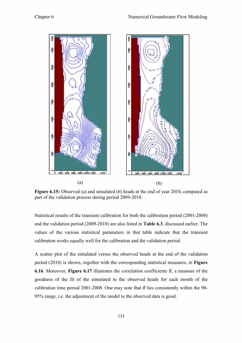
Chapter 6 Numerical Groundwater Flow Modeling
133
(a)
(b)
Figure 6.15: Observed (a) and simulated (b) heads at the end of year 2010, computed as part of the validation process during period 2009-2010.
Statistical results of the transient calibration for both the calibration period (2001-2008)
and the validation period (2009-2010) are also listed in Table 6.3, discussed earlier. The
values of the various statistical parameters in that table indicate that the transient
calibration works equally well for the calibration and the validation period.
A scatter plot of the simulated versus the observed heads at the end of the validation
period (2010) is shown, together with the corresponding statistical measures, in Figure
6.16. Moreover, Figure 6.17 illustrates the correlation coefficients R, a measure of the
goodness of the fit of the simulated to the observed heads for each month of the
calibration time period 2001-2008. One may note that R lies consistently within the 90-
95% range, i.e. the adjustment of the model to the observed data is good.

Chapter 6 Numerical Groundwater Flow Modeling
134
Figure 6.16: Scatter plot of calculated over observed heads and summary of transient calibration statistics for year 2010.
Figure 6.17: Monthly correlation coefficient for the calibration period 2001-2008.
Table 6.5 presents the final calibrated aquifer parameters values found from these
calibration runs.
87
88
89
90
91
92
93
94
95
96
97
Cor
rela
tion
coe
ff. (
R)
%
Month
R (2001) R (2002) R (2003) R (2004)
R (2005) R (2006) R (2007) R (2008)

Chapter 6 Numerical Groundwater Flow Modeling
135
Table 6.5: Finally calibrated aquifer parameters for the groundwater flow model.
Parameter Sub-aquifer Aquitard Unit
kxx (conductivity in x direction) 34
3.94 E-4 0.2
2.3 E-6 m/d m/s
kyy (conductivity in y direction) 34
3.94 E-4
0.2
2.3 E-6
m/d
m/s
kzz (conductivity in z direction) 3.4
3.94 E-5
0.02
2.3 E-7
m/d
m/s
Sy (Specific yield) 0.18 0.05 -
Ss (Specific storage) 10-4 10-5 m-1
Ф (Effective porosity) 0.25 0.3 -
n (Total porosity) 0.3 0.45 -
The three panels of Figure 6.18 show observed and calibrated yearly groundwater
levels for wells E45, Pzo36A and L57, located in the north, the middle and the south of
Gaza, respectively, over time, for both the calibration period 2001-2008 and the
validation period 2009-2010. These well hydrographs indicate that the observed heads
are well mimicked by the simulations, up to a discrepancy, that, in most cases, does not
exceed 0.5 m.
Groundwater flow balance calculations have also been carried out for the transient
simulations. These can help to understand the effects of several influential factors,
including pumping rate (discharge), seasonal fluctuations in recharge and storage
change. Figure 6.19 shows the average annual total discharge, recharge and storage
change for the aquifer system during the total transient time period 2001-2010. From the
figure one may notice that the regional storage change has become permanently
negative after 2001, which means that the aquifer has continuously been depleted since
that time.
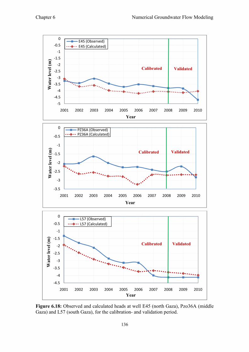
Chapter 6 Numerical Groundwater Flow Modeling
136
Figure 6.18: Observed and calculated heads at well E45 (north Gaza), Pzo36A (middle Gaza) and L57 (south Gaza), for the calibration- and validation period.
-5
-4.5
-4
-3.5
-3
-2.5
-2
-1.5
-1
-0.5
0
2001 2002 2003 2004 2005 2006 2007 2008 2009 2010
Wa
ter
lev
el (
m)
Year
E45 (Observed)E45 (Calculated)
Calibrated Validated
-3.5
-3
-2.5
-2
-1.5
-1
-0.5
0
2001 2002 2003 2004 2005 2006 2007 2008 2009 2010
Wat
er le
vel
(m)
Year
PZ36A (Observed)PZ36A (Calculated)
Calibrated Validated
-4.5
-4
-3.5
-3
-2.5
-2
-1.5
-1
-0.5
0
2001 2002 2003 2004 2005 2006 2007 2008 2009 2010
Wat
er le
vel
(m)
Year
L57 (Observed)L57 (Calculated)
ValidatedCalibrated

Chapter 6 Numerical Groundwater Flow Modeling
137
Figure 6.19: 2001-2010 annual simulated discharge, recharge and storage change in the Gaza aquifer.
6.4.2. Model sensitivity analysis
A model sensitivity analysis has also been carried out, in order to evaluate the effects of
uncertainties in various input parameters of the numerical model, such as, for example,
the boundary conditions, aquifer parameters and stresses, on the output of the calibrated
model (e.g. Anderson and Woessner, 1992). As a matter of fact, even if the boundary
conditions and the conceptual model are exactly known, uncertainties in the model
parameters would still cause predictions error.
Sensitivity is expressed here by a dimensionless index SI, calculated as the ratio
between the relative (absolute) change of model output |Δy|/y0 and the relative change
of an input parameter Δx/x0, i.e. SI = (|Δy|/y0) / (Δx/xo) (e.g. Lenhart et al., 2002;
Arlai et al., 2006). The calculated sensitivity indices are ranked into four classes, as
shown in Table 6.6, and this ranking is used to assess the calculated sensitivities and to
support the results.
The sensitivity tests have been carried out here with the focus on the two input
parameters hydraulic conductivity and recharge, which are known to have significant
and, often, adverse impacts on the simulated heads. During these sensitivity runs the
-100
-50
0
50
100
150
200
250
2000 2001 2002 2003 2004 2005 2006 2007 2008 2009 2010 2011
Ch
an
ge
Ra
te (
MC
M)
Year
Total Discharge
Total Recharge
Storage change

Chapter 6 Numerical Groundwater Flow Modeling
138
values of these two variables have been changed separately between +/-30 %, with an
increment rate of +/-10 %, from their previously determined optimal reference values,
with the other variable kept constant. Meanwhile, the hydraulic conductivity k for the
three aquitard layers is changed from 0.05 m/d to 0.4 m/d, wherefore the k of the
calibrated reference case is 0.2 m/d.
Table 6.6: Ranking of sensitivity classes (Lenhart et al., 2002).
Class Index Sensitivity
I 0.00 ≤ | I | ≤ 0.05 Small to neglect
II 0.05 ≤ | I | ≤ 0.2 Medium
III 0.20 ≤ | I | ≤ 1.00 High
IV | I | ≥ 1.00 Very high
Tables 6.7 and 6.8 summarize the statistical results of the sensitivity analysis for the
hydraulic conductivities of the sub-aquifers and the aquitards, respectively, while Table
6.9 shows the corresponding results for the sensitivity of the groundwater recharge.
Table 6.7: Sensitivity analysis for the hydraulic conductivity k of the sub-aquifers.
Change in k (%)
Correlation coefficient
Absolute residual mean (m)
|��|/y0 ��/�� Sensitivity index (S)
Sensitivity
class
-30 0.92 1.13 0.36 -0.3 -1.2 Very high
-20 0.92 0.98 0.18 -0.2 -0.9 High
-10 0.92 0.89 0.07 - 0.1 - 0.70 High
Reference 0.92 0.83 - - - -
+10 0.92 0.8 0.04 0.1 0.40 High
+20 0.92 0.79 0.05 0.2 0.25 High
+30 0.92 0.79 0.05 0.3 0.16 Medium

Chapter 6 Numerical Groundwater Flow Modeling
139
Table 6.8: Sensitivity analysis for the hydraulic conductivity k of the aquitards.
Change in k (m/d)
Correlation coefficient
Absolute residual
mean (m) |��|/y0 ��/��
Sensitivity index (S)
Sensitivity
class
0. 05 0.92 0.834 0.005 - 0.75 - 0.006 Small to neglect
0.1 0.92 0.829 0.001 - 0.5 0.002 Small to neglect
0.2 (reference) 0.92 0.83 - - - -
0.3 0.92 0.825 0.006 0.5 0.01 Small to neglect
0.4 0.92 0.824 0.007 1.0 0.007 Small to neglect
Table 6.9: Sensitivity analysis for the recharge R.
Change in R (%)
Correlation coefficient
Absolute residual
mean (m) |��|/y0 ��/��
Sensitivity index (S)
Sensitivity
class
-30 0.90 1.35 0.62 -0.3 -2.07 Very high
-20 0.91 1.14 0.37 -0.2 -1.85 Very high
-10 0.92 0.97 0.17 -0.1 -1.68 Very high
Reference 0.92 0.83 - - - -
+10 0.92 0.73 1.00 0.1 0.99 High
+20 0.92 0.70 0.19 0.2 0.95 High
+30 0.90 0.74 0.1 0.3 0.36 High
Figure 6.20 shows that the model is more sensitive to lower values of the hydraulic
conductivity, or of the recharge, than to higher values, as the sensitivity indices SI are
higher for the former than for the latter. This can also be seen from Figure 6.21, where
the absolute changes of the various error estimates of the model, discussed

Chapter 6 Numerical Groundwater Flow Modeling
140
Figure 6.20: Sensitivity index as a function of the change in hydraulic conductivity (top) and of the recharge (bottom).
earlier, namely, the residual mean (RM), the absolute residual mean (ARM) and the root
mean square error (RMS) are plotted as a function of the respective percentile parameter
change. Thus, one may note that with increasing hydraulic conductivity or recharge all
three calibration measures are decreasing.
Figure 6.21 also points out to the well-known problem, found also in other groundwater
modeling studies (e.g. Arlai et al., 2012; Koch et al., 2012), namely, the existence of
some amount of trade-off, or ambiguity, in the two varied aquifer parameters, hydraulic
-1.2
-1
-0.8
-0.6
-0.4
-0.2
0
0.2
0.4
-30 -20 -10 0 10 20 30
Sen
siti
vit
y In
dex
(S
I)
Change in hydraulic conductivity in percentage
-1.80
-1.40
-1.00
-0.60
-0.20
0.20
0.60
1.00
-30 -20 -10 0 10 20 30
Sen
siti
vity
In
dex
(S
I)
Change in Recharge in percentage
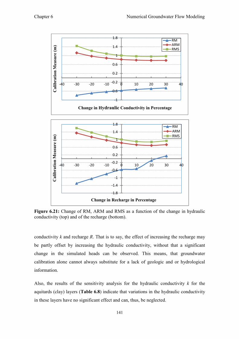
Chapter 6 Numerical Groundwater Flow Modeling
141
Figure 6.21: Change of RM, ARM and RMS as a function of the change in hydraulic conductivity (top) and of the recharge (bottom).
conductivity k and recharge R. That is to say, the effect of increasing the recharge may
be partly offset by increasing the hydraulic conductivity, without that a significant
change in the simulated heads can be observed. This means, that groundwater
calibration alone cannot always substitute for a lack of geologic and or hydrological
information.
Also, the results of the sensitivity analysis for the hydraulic conductivity k for the
aquitards (clay) layers (Table 6.8) indicate that variations in the hydraulic conductivity
in these layers have no significant effect and can, thus, be neglected.
-1
-0.6
-0.2
0.2
0.6
1
1.4
1.8
-40 -30 -20 -10 0 10 20 30 40
Ca
lib
rati
on
Mea
sure
(m
)
Change in Hydraulic Conductivity in Percentage
RMARMRMS
-1.8
-1.4
-1
-0.6
-0.2
0.2
0.6
1
1.4
1.8
-40 -30 -20 -10 0 10 20 30 40
Cal
ibra
tion
Mea
sure
(m
)
Change in Recharge in Percentage
RMARMRMS

Chapter 6 Numerical Groundwater Flow Modeling
142
6.5. Conclusions
This chapter has outlined the development and application of a numerical groundwater
flow model, based on the 3D- finite difference model MODFLOW, as embedded in the
Visual MODFLOW software environment, to the Gaza coastal aquifer.
The optimal MODFLOW-model for predicting groundwater levels in the Gaza coastal
aquifer is developed in two major steps. In the first step, steady-state calibrations for
year-2000 observed hydraulic heads have been carried out, by adjusting the hydraulic
conductivity/transmissivity, as well as the amount of natural recharge. A good
agreement between simulated and observed groundwater levels, with a correlation
coefficient of R = 0.92, is obtained.
In the second step, transient head simulations for years 2001-2010 have been carried
out, wherefore the time period 2000-2008 is used to calibrate the storage coefficients
and the specific yield of the aquifer and the remaining time for the verification of the
model. Again a good agreement between simulated and observed groundwater levels is
achieved for both the calibration period 2001-2008 and the validation period 2009-2010,
with a correlation coefficient of R = 0.938. The head results, as well as the water budget
results, show that the physical groundwater situation in the region has been
continuously deteriorating over the last decade, as groundwater levels have dropped by
nearly 5 m and 10 m in two major pumped areas in northern and southern Gaza,
respectively, and storage changes have become increasingly negative in recent years.
The subsequent sensitivity analysis of the calibrated groundwater flow model shows
that the simulated heads are more sensitive to lower than to higher values of both the
hydraulic conductivity and recharge. At the same time, some amount of trade-off
between these two parameters is found, i.e. they cannot be determined independently in
a unique way.

Chapter 7 Modeling of seawater intrusion in the Gaza aquifer
143
Chapter 7 : Numerical Modeling of the Saltwater Intrusion into the Gaza Coastal Aquifer using a Variable-Density Flow and Transport Model
7.1. General remarks on the modeling of variable-density flow and transport
In coastal aquifers, because of non-uniform distributions of highly concentrated solutes,
as in seawater, corresponding large density variations in the saline groundwater arise
which, in turn, have an effect on the groundwater flow movement. This means that,
unlike in constant-density groundwater flow and solute transport modelling, where the
flow is not affected any more by the subsequent concentration solution of the transport
equation, for variable-density flow and transport the groundwater flow equation and the
solute transport equation are coupled with each other by an equation of state for the
density as a function of the solute concentration. Therefore, groundwater flow cannot be
computed once and for all over the whole simulation period, after which for the former
can then be used for the advancement of the solute front, but, instead, the flow must be
recomputed in each time step, using updated concentrations from the transport equation,
and with it, updated densities. All this makes the modeling of variable-density
groundwater flow and solute transport a much harder computational task than regular
solute transport modeling.
In spite of these intricacies, computer modelling of density-dependent flow and solute
transport has become nowadays a powerful tool for understanding and analyzing the
hydrology of groundwater aquifers and various other aspects of subsurface flow and
transport processes, such as seawater intrusion. Thus, numerous theoretical and applied
studies exist to this date (Bear, 1961; Bachmat, 1967; Pinder and Cooper, 1970; Bear,
1979; Andersen et al., 1988; Essaid, 1990; Rivera et al., 1990; Fetter 1994; Calvache
and Pulido-Bosch 1994; Gangopadhyay and Gupta 1995; Huyakorn et al., 1996; Bear et
al., 1999; Zhou et al., 2000a: Langevin, 2001; Zhang and Brusseau, 2004; Langevin et
al., 2005; Schaars et al., 2011). Particular density-dependent flow and solute transport
models to be mentioned here (see also Chapter 2) are the SUTRA model (Voss, 1984)
and the more recently developed SEAWAT model (Guo and Bennett, 1998; Guo, &

Chapter 7 Modeling of seawater intrusion in the Gaza aquifer
144
Langevin, 2002; Langevin, 2003) which is based on the MODFLOW/MT3D constant-
density flow and transport model (McDonald and Harbaugh, 1988; Zheng, 1990).
The work presented in this chapter is an extension of previous seawater intrusion
modeling studies in the Gaza aquifer, which have already been discussed in chapter 2.
The SEAWAT model will also be applied in this chapter of the thesis to simulate the
seawater intrusion process in the Gaza coastal aquifer. More specifically, whereas in
this chapter the calibrated SEAWAT model will be applied to the modeling of the
present-day and future behavior of the seawater intrusion, the emphasis in the
subsequent chapter will be on the simulation of the future development of the intrusion
front under various groundwater management scenarios as a tool for sustainable
quantitative and qualitative management of the groundwater resources in the Gaza
coastal aquifer.
7.2. SEAWAT modeling approach
7.2.1. General features of SEAWAT
SEAWAT was originally written by Guo and Bennett (1998) to simulate three-
dimensional, variable-density ground water flow. SEAWAT was designed, following
closely the modular structure of the (constant-density) coupled flow model
MODFLOW (McDonald and Harbaugh, 1988) and the solute-transport model MT3D
(MT3DMS) (Zheng, 1990), but allowing for a two-side coupling of the effects of solute
concentration on the density of fluid flow and vice versa.
More particularly, the original MODFLOW- model is modified in the SEAWAT-
version such that fluid mass rather than fluid volume is conserved and Darcy's equation,
driving variable-density flow, is written in terms of an "equivalent freshwater head" as
the principal dependent variable. Using this fundamental concept, most of the basic
structures of the original (density-independent) MODFLOW code are kept intact, which
also means that a calibrated MODFLOW groundwater model, as developed for the Gaza
coastal aquifer in the previous chapter, can essentially be used unaltered in SEAWAT,
which may be considered as one of its most advantageous feature. However, unlike in a
constant-density flow and transport model, in which there is no feedback of the
computed solute concentration on the flow, so that the latter can be computed upfront

Chapter 7 Modeling of seawater intrusion in the Gaza aquifer
145
for the total simulation period, the flow solution from SEAWAT is passed in each
timestep to the MT3DMS solute transport model, to compute a new solute concentration
which is then used to compute new densities that, in return, are fed back into
MODFLOW. These updated densities are then used for the computation of the flow,
either for the next time-step, or when density changes are too big, for the same timestep
and, so, repeating the concentration simulation in another sub-cycle (Guo and Langevin,
2002). These two options are called explicit or implicit coupling of the groundwater
flow equation with the solute-transport equation, respectively.
7.2.2. SEAWAT theoretical details
7.2.2.1. Concept of equivalent freshwater head
Calculation of the hydraulic head gradient is the first step in solving a density-driven
flow and transport problem in a coastal aquifer system. However, due to the presence of
the non-uniform fluid densities, because of varying saltwater concentrations, the
concept of hydraulic head is not straightforward. For example, the total hydraulic
(freshwater) head hf measured just above a saltwater/freshwater interface would yield a
different value than the total hydraulic (saltwater) head h measured just below the
interface, because of these density differences.
SEAWAT is based on the concept of equivalent freshwater head hf in a saline ground-
water environment, whereby all equations are written in terms of one hf whose effective
value depends on the local, true, variable density at the same location.
For a thorough understanding of the term of equivalent freshwater head, two
piezometers open to a given point N in an aquifer, containing saline water, are shown in
Figure 7.1. Piezometer A contains freshwater and is equipped with a mechanism that
prevents saline water in the aquifer from mixing with freshwater. Piezometer B contains
water identical to that present in the saline aquifer at point N (Guo and Langevin, 2002).
The total hydraulic head hf measured at point N just above the freshwater/saltwater
interface is expressed in the usual way as

Chapter 7 Modeling of seawater intrusion in the Gaza aquifer
146
ℎ� = ��
��
� + �� (7.1)
where: hf , the equivalent freshwater head [L], PN, the pressure at point N [ML-1T-2], ρf the density of freshwater [ML-3], g, the acceleration due to gravity [LT-2] and ZN, the elevation of point N above datum [L].
An equivalent expression is found for the total (saline) hydraulic head h, measured at
point N just below the interface:
ℎ = ��
��+ �� (7.2)
where: h, head [L] ρ, density of saline ground water at point N [ML-3]. Solving Eqs, (7.1) and (7.2) for PN results in
�� = ��� (ℎ� – �) (7.3)
�� = �� (ℎ – �)
(7.4)
whereby the datum ZN has been replaced by the more general datum Z. Setting (7.3) and (7.4) equal to each other, two conversion formulae expressing one
head by the other and vice versa:
ℎ� = ���
ℎ − � − ��
��
� (7.5)
ℎ = ��
�ℎ� +
� − ��
� � (7.6)

Chapter 7 Modeling of seawater intrusion in the Gaza aquifer
147
Figure 7.1: Illustration of the principle of the equivalent freshwater head (Guo and Langevin, 2002).
Where, in SEAWAT, the second equation is mainly used, i.e., the total head h appearing
in the Darcy equation and the pressure P in the groundwater balance equation is written
in terms of the equivalent freshwater head hf. This approach conserves the basic
structure of the fundamental equations and, so, allows practically the use of the same
software, such as MODFLOW, with relatively little modification.

Chapter 7 Modeling of seawater intrusion in the Gaza aquifer
148
7.2.2.2. Governing equations
The density-dependent groundwater flow equation
Using the previously discussed concept of the equivalent total freshwater head, the
groundwater flow equation for variable density flow can be written in terms of this fresh
water head, as follows (Langevin et al., 2003):
�
������� �
���
���� +
∂
∂y����� �
∂ℎ�
∂y�� +
∂
∂z����� �
∂ℎ�
∂z+ �
�−��
���
∂Z
∂z��
= ��� ���
��+ �
��
��
��
��− ρsqs
(7.7)
where:
hf, equivalent fresh water head [L].
kfx, kfy, kfz, equivalent freshwater hydraulic conductivities in the three coordinate
directions [LT-1].
ρ, density of native aquifer water [M/L3]
ρf, density of freshwater [M/L3].
Sf, specific storage in term of equivalent fresh water head [L-1].
C, solute concentration [M/ L3].
�, effective porosity (dimensionless).
ρs, density of water entering from a source or leaving through a sink [M/L3].
qs, volumetric flow rate of sources or sinks per unit volume of aquifer [T-1].
The rate of the groundwater flow is characterized by the average linear pore water
velocity (seepage velocity) v, which can be computed by Darcy’s law:
v = k/ne * grad h
where,
v, average linear pore water velocity vector (L/T), k, hydraulic conductivity (L/T), ne, effective porosity of the porous media (dimensionless), grad h, hydraulic gradient of the head h (defined in terms of the freshwater head hf) .
(7.8)
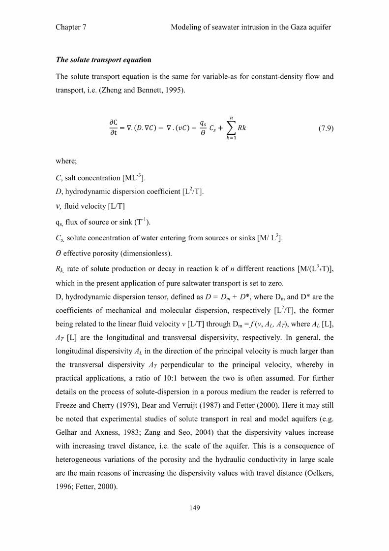
Chapter 7 Modeling of seawater intrusion in the Gaza aquifer
149
The solute transport equation
The solute transport equation is the same for variable-as for constant-density flow and
transport, i.e. (Zheng and Bennett, 1995).
∂C
∂t= ∇. (�. ∇�) − ∇ . (��) −
��
� �� + � ��
�
���
(7.9)
where;
C, salt concentration [ML-3].
D, hydrodynamic dispersion coefficient [L2/T].
v, fluid velocity [L/T]
qs, flux of source or sink (T-1).
Cs, solute concentration of water entering from sources or sinks [M/ L3].
� effective porosity (dimensionless).
Rk, rate of solute production or decay in reaction k of n different reactions [M/(L3*T)],
which in the present application of pure saltwater transport is set to zero.
D, hydrodynamic dispersion tensor, defined as D = Dm + D*, where Dm and D* are the
coefficients of mechanical and molecular dispersion, respectively [L2/T], the former
being related to the linear fluid velocity v [L/T] through Dm = f (v, AL, AT), where AL [L],
AT [L] are the longitudinal and transversal dispersivity, respectively. In general, the
longitudinal dispersivity AL in the direction of the principal velocity is much larger than
the transversal dispersivity AT perpendicular to the principal velocity, whereby in
practical applications, a ratio of 10:1 between the two is often assumed. For further
details on the process of solute-dispersion in a porous medium the reader is referred to
Freeze and Cherry (1979), Bear and Verruijt (1987) and Fetter (2000). Here it may still
be noted that experimental studies of solute transport in real and model aquifers (e.g.
Gelhar and Axness, 1983; Zang and Seo, 2004) that the dispersivity values increase
with increasing travel distance, i.e. the scale of the aquifer. This is a consequence of
heterogeneous variations of the porosity and the hydraulic conductivity in large scale
are the main reasons of increasing the dispersivity values with travel distance (Oelkers,
1996; Fetter, 2000).

Chapter 7 Modeling of seawater intrusion in the Gaza aquifer
150
In fact, Eq. (7.9) is the so-called advection-dispersion equation which describes the
transport of solutes in a general fluid flow (described by its flow velocity v, which in the
present application is equal to the groundwater flow velocity v). The transport by the
flow alone is called the advective transport and is represented by the second term on the
right side of the equation. The first term on the right side represents solutes
concentration change due to hydrodynamic dispersion and the other terms have been
discussed above.
Equation of state relating density to concentration
The variable density flow equation (7.7) is coupled in two ways to the transport
equation (7.9). Firstly by the second term on the right-hand side of Eq. (7.7) which
represents the change of fluid mass due to the change in solute concentration C, and,
secondly, by the direct effect of C on the density ρ appearing on the left side of the
subsequent equation.
The empirical (linear to first order) relation between the density ρ of saltwater and
concentration C, also called an equation of state, was developed by Baxter and Wallace
(1916) and can be written as
� = �� + ��
(7.10)
where: E= dρ/dc is the empirical relation between the density and salt concentration, and which
has a value of E= 0.7143 for salt concentrations ranging between zero and that of
seawater. With Eq. (7.10) the groundwater flow equation (7.7) is coupled to the solute
transport equation (7.9).
7.2.3. SEAWAT computational procedures
Likewise to the underlaying MODFLOW/MT3D- models, on which SEAWAT is based,
stress periods are divided into smaller timesteps, whereby the timestep lengths are
calculated during the simulation by SEAWAT, to satisfy the stability constraints and
accuracy requirements for the transport of conservative species (advection) using an

Chapter 7 Modeling of seawater intrusion in the Gaza aquifer
151
Figure 7.2: Generalized flow chart of the SEAWAT coupling procedure (Guo and Langevin, 2002).
explicit finite-difference schemes, which means that the number of timesteps is not
known prior to execution. As discussed earlier, unlike in constant-density flow and
transport modeling, now both the flow and transport equations are solved during one
SEAWAT timestep.
Moreover, in SEAWAT the coupling between flow and transport is performed through a
synchronous timestepping approach that cycles between MODFLOW solutions of the
flow equation and MT3DMS solutions of the transport equation, using an iterative
computational process (Figure 7.2).
In a first step, the groundwater flow equation is solved for the head and, using Darcy's
law, the velocity field is computed. This velocity is then passed to the transport equation
which calculates the solute transport during that time step. The density field is then
updated via the equation of state (Eq. 7.10) and the heads are recalculated with the flow

Chapter 7 Modeling of seawater intrusion in the Gaza aquifer
152
equation. This iterative procedure is continued until the density difference is less than
some user-specified density value. More specifically, the SEAWAT program includes
two methods for coupling the flow and solute-transport equations, namely, an explicit
and an implicit method.
In the (simpler) explicit method, the flow equation is solved first for each timestep, and
the resulting advective velocity field is then used in the solution of the solute-transport
equation. Then the flow equation is advanced in time, using the updated density and the
concentrations from the previous time step, which means that the values of these two
variables are always lagging behind by one time step. This computationally fast "one-
iteration" cycle, or explicit approach, works only properly, if the timesteps are small
enough to avoid large density- and concentration changes will not arise. However, if the
latter are becoming too large, inaccuracies and even instabilities in that solution
procedure may occur.
Meanwhile, in the implicit coupling method, solutions to the flow and transport
equations are computed multiple times for the same timestep, with the concentrations
and densities are updated within this timestep, until the differences in fluid density at
each cell of the model domain are less than a user-specified density value. In fact, the
implicit coupling approach in SEAWAT only works when a MT3DMS finite-difference
method is used to solve the solute-transport equation. As the implicit finite-difference
approach is known to have a larger numerical stability range, larger time steps can be
also taken for the solution of the transport equation.
In the present application of SEAWAT-model, the implicit coupling approach has been
used, which is more appropriate, especially, for seawater intrusion problems, where the
fluid density contrasts are not that large (~2.5%), which may vary between freshwater
(�=1000 kg/m3) and seawater (�=1025 kg/m3), i.e. which is much less than what can be
expected when modeling brines (� > 1500 kg/m3).

Chapter 7 Modeling of seawater intrusion in the Gaza aquifer
153
7.3. SEAWAT model set-up for the Gaza coastal aquifer
7.3.1. Set-up of the groundwater flow module
As the basic conceptual structure of the groundwater flow model part of SEAWAT is
essentially identical to the MODFLOW model, the conceptual model setup of
SEAWAT for the Gaza coastal aquifer, as implemented in Visual MODFLOW, relies
directly also on that of the original MODFLOW groundwater flow model set-up,
presented in detail in Chapter 6 (see also Sirhan and Koch, 2013a). Therefore, a
thorough discussion of that part of the SEAWAT modeling task is omitted here. This
means also that the calibration results of the constant-density MODFLOW-2000 model,
as well as the main internal and external hydrologic sources and stresses, will be
incorporated with only minor adjustments into the SEAWAT-2000 variable-density
model, to simulate the transient dynamics of the saltwater-freshwater interface in the
Gaza coastal aquifer.
7.3.2. Boundary conditions (solute transport module)
In addition to the boundary conditions already assigned in the conceptual Gaza aquifer
groundwater flow model of Chapter 6, boundary conditions have also to be applied for
the solution of the solute transport equation in the model domain. These are, namely,
constant concentration (Dirichlet) boundaries in the west (coastline), with a constant salt
concentration equivalent to that of seawater (see subsection below), and Neumann
boundary conditions in the east, with a specified salt concentration (see Figure 6.3 for
details):
Dirichlet boundary-conditions with a constant salt (TDS) concentration of that
of seawater, i.e. C=C0 = 35,000 mg/l (salinity) are set in all layers for all cells
along the Gaza coastline.
Neumann boundary conditions with a TDS of 250-1100 mg/l (salinity) are
assigned in all layers for all cells at the eastern boundary.
The salinization due to the infiltration of contaminant water from the surficial recharge
(rainfall) is neglected, because of its very small effect, compared to the main source of
salinity i.e. seawater intrusion.

Chapter 7 Modeling of seawater intrusion in the Gaza aquifer
154
7.3.3. Initial conditions
For the transient variable-density groundwater flow and solute transport simulations,
which cover a time period of 2001-2010, initial conditions for chloride concentrations
distributed across the model area must be set. In the present application the simulated
chloride concentrations for year 2000, as obtained during the steady-state calibration of
the model, are assigned as initial condition for the transient simulation.
In fact, SEAWAT model requires the concentrations of total dissolved solids (TDS)
which, by virtue of the equation of state (Eq. 7.10), determines the density of the saline
fluid, rather than the chloride concentrations. Therefore, the latter are linearly converted
to TDS, by assuming that seawater has a chloride concentration of 19,800 mg/l and a
TDS value of 35,000 mg/l (Parker et al., 1955). This means then also, that the
SEAWAT-computed concentration output is discussed in terms of total salinity, not
chloride concentrations.
7.3.4. Exploitation of the calibrated parameters of the constant-density flow
model in the variable-density SEAWAT-model
After successful calibration of the 3D- MODFLOW FD (constant-density) groundwater
flow model (see Chapter 6 and Sirhan and Koch, 2013a), the density-dependent flow
and solute transport model SEAWAT-2000, as implemented in Visual MODFLOW, has
been set up, using the same conceptual model, while exploiting the already calibrated
aquifer parameters of that flow model, to simulate the dynamics of the seawater–
freshwater interface.
More specifically, most of the data and the earlier calibrated hydraulic parameters, such
as the horizontal hydraulic conductivity Kxx and Kyy, the vertical hydraulic conductivity
Kzz, the specific yield Sy and the specific storage Ss are also used in the variable-density
model SEAWAT. As discussed in Chapter 6 (see Table 6.5), for the Gaza aquifer
system, the three hydraulic conductivities Kxx, Kyy and Kzz are such that Kxx = Kyy ≠ Kzz,,
i.e. the aquifer system is assumed to be transversely isotopic.
Regarding the solute transport parameters, required in the solute transport equation
(7.9), namely, the hydrodynamic dispersivities AL and AT for the sub-aquifers and

Chapter 7 Modeling of seawater intrusion in the Gaza aquifer
155
aquitards, these have initially been assigned and are then adjusted by trial and error
during the subsequent model calibrations. As mentioned earlier, the longitudinal
dispersion is much larger than the transversal dispersion (e.g. Gelhar and Axness, 1983;
Fetter, 2000), so that in line with many other solute transport studies on the field scale
(Gelhar et al., 1992; Sorek, et al., 1998; Yakirevich et al., 1998: Metcalf & Eddy,
2000), the initial longitudinal dispersivity AL has been assigned a value of 10-12 m, the
transverse dispersivity AT in the horizontal direction a value of 1-2 m, and the
transverse dispersivity AT in the vertical direction a value of 0.1-0.2 m. For the
molecular diffusivity D*, a value of diffusion coefficient of 1×10⁻¹⁰ m2/day can be used,
but due to the fact that molecular diffusion is an insensitive parameter, it can be ignored
in the salinity calibration (Langevin et al., 2008).
7.4. Validation of the SEAWAT flow module
The validation of the SEAWAT model calibration is an important step, which allows to
get more confidence in this variable-density flow and transport model, using the set of
calibrated parameter values and stresses from the previously calibrated constant-density
groundwater flow model in the variable-density model. This validation consists mainly
in the check of the SEATWAT model results against the calibrated hydraulic parameters
of the aquifer system by history matching of the observed hydraulic heads under steady-
state and transient conditions.
Although the SEAWAT model could already have been applied directly for the
calibration of the groundwater flow in the Gaza aquifer, instead of the MODFLOW
model in Chapter 6, for some didactic reasons, namely, the constant-density
simplification and the easier-to-use interface of the latter, as implemented in the Visual
MODFLOW software, the original MODFLOW model has been chosen and applied in
this initial stage of the groundwater flow and seawater intrusion investigation.
7.4.1. Steady-state validation
For the steady-state validation of the SEAWAT model, year-2000 head data have been
used as targets. The results for the "variable-density" heads are presented in terms of
both a qualitative and a quantitative assessment. A qualitative picture is obtained from
Figure 7.3, where the observed, MODFLOW-simulated and SEAWAT-validated head

Chapter 7 Modeling of seawater intrusion in the Gaza aquifer
156
(a) (b) (c)
Figure 7.3: Observed (a), MODFLOW-simulated (b) and SEAWAT-validated (c) year-2000 heads for steady-state calibration.
isolines for year 2000 are shown. It is obvious that the validated SEAWAT model
simulates the aquifer system well, as its head isolines have a very similar pattern as both
the observed and the MODFLOW (constant-density) simulated heads.
Similar to the MODFLOW calibrations (see Chapter 6), a more quantitative assessment
of the SEAWAT-validation is gained from various statistical error estimates (residuals)
of the fit of the observed heads by the validated model, namely, (1) the mean residual (=
- 0.506), (2) the mean absolute residual (= 0.832), (3) the standard error of the estimate
(= 0.124) and (4) the root mean square error (MSE= 1.004). A scatter plot of the
calculated versus the observed heads is shown in Figure 7.4, which reveals that the
model fits the model fits the observed groundwater levels rather well, as all points are
lying close to the diagonal line, with a correlation coefficient R = 0.923.

Chapter 7 Modeling of seawater intrusion in the Gaza aquifer
157
Figure 7.4: Scatterplot of calculated over observed year 2000 heads for SEAWAT- steady-state validation for the various layers of the model with statistical summary.
7.4.2. Transient validation
Similar to the steady-state validation, a very good agreement, both qualitatively and
quantitatively, between observed and simulated heads is obtained in the transient
SEAWAT-validation models. Figure 7.5 shows the head isolines pattern obtained at the
end of year 2010. It is obvious that the "variable-density" computed heads of SEAWAT
have similar pattern as both the observed and the MODFLOW-simulated one. In
particular, the two groundwater head depression cones observed in the north and south
of the Gaza strip are also well mimicked by the SEAWAT- model.
Similar to Figure 7.4, the quantitative scatterplot of the SEAWAT-computed over the
observed heads at the end of the transient simulation period (2000-2010) is shown in
Figure 7.6, together with the corresponding statistical measures, namely, (1) the mean
residual (= 0.816), (2) the mean absolute residual (= 1.47), (3) the standard error of the
estimate (= 0.229) and (4) the root mean square error (MSE= 1.8). Table 7.1
summarizes the various statistical error estimates obtained again, as well as those
obtained in the steady-state-, transient calibration and SEAWAT-validation. The high

Chapter 7 Modeling of seawater intrusion in the Gaza aquifer
158
(a) (b) (c)
Figure 7.5: Observed (a), MODFLOW-simulated (b) and SEAWAT-validated (c) heads at the end of year 2010 computed in transient mode for time-period 2001-2010.
correlation coefficient R=0.914, in particular, reveals that the SEAWAT-model fits the
observed groundwater levels rather well, as all points are lying close to the diagonal line
and inside the 95% confidence interval .
A comparison between the MODFLOW-simulation and SEAWAT-validation is shown
in Table 7.1. Thus, one may conclude from this table that the SEATWAT model results
obtained for the various statistical error estimates for the steady-state validation are
similar to those of the MODFLOW-simulation, while for the transient simulations the
MODFLOW-model appears to provide better results than the SEAWAT-validation. At
this stage it cannot be ruled out that a better calibration of the SEAWAT-model could
also be obtained by an independent trial-and-error calibration of SEAWAT, however,
for the reasons discussed earlier, in particular, the time-consuming efforts and the

Chapter 7 Modeling of seawater intrusion in the Gaza aquifer
159
Figure 7.6: Scatterplot of transient SEAWAT- calculated over observed heads at the end of year 2010 for the various layers of the model with summary of statistics.
Table 7.1: Statistics for MODFLOW/ SEAWAT steady-state and transient calibrations
Statistical parameter MODFLOW
steady- state
2000
SEAWAT
steady- state
2000
MODFLOW
transient simulation
2001-2010
SEAWAT
transient validation
2001-2010
Num. of observation wells 114 114 50 50
Mean residual (m) - 0.57 - 0.506 0.011 0.816
Mean abs. residual (m) 0.83 0.832 0.906 1.47
Std. error of estimate (m) 0.08 0.124 0.164 0.229
RMS (m) 1.01 1.004 1.146 1.79
Normalized RMS (%) 5.6 6.93 5.743 6.408
Correlation coefficient 0.92 0.923 0.938 0.914
complexities typically associated with building up a three-dimensional groundwater
flow and contaminant transport model with the SEWAT-code, make the use of a
constant-density groundwater flow MODFLOW model still preferable.

Chapter 7 Modeling of seawater intrusion in the Gaza aquifer
160
7.5. Calibration of the SEAWAT- solute transport model
Similar to the calibration and validation procedure for the groundwater flow modul of
SEAWAT, discussed on the previous sections, and following the usual approach in
groundwater flow and transport modeling (e,g. Anderson and Woessner, 1992), both
steady-state and transient calibrations for the solute transport modul, of SEAWAT,
wherefore chloride concentrations measured biannually in the 2000-2010 time period at
51 wells distributed across the model area (see Chapter 4) are used as calibration
targets, have been carried out. More exactly, as in the SEAWAT- model, the TDS
salinity is required, all chloride concentrations are converted to equivalent TDS-
salinity, prior use in the subsequent processing.
In addition to the aquifer parameters already calibrated in the groundwater flow model
(Chapter 6 and Sirhan and Koch, 2013a), the dispersivities for the sub-aquifers and
aquitards (clay) layers are adjusted by trial and error in the transient calibration of the
SEAWAT solute transport model, within the ranges, as listed in Table 7.2.
Table 7.2: Calibration ranges of the dispersivities for the solute transport model.
Parameter Sub-aquifer Aquitard Unit
Longitudinal dispersivity (AL) 10 - 20 0.5 - 2 m
Horizontal transverse dispersivity (AT) 1- 2 0.05 – 0.2 m
Vertical transverse dispersivity 0.1 – 0.2 0.005 - 0.02 m
7.5.1. Steady-state salinity calibration
The results of the steady-state calibration are presented both in terms of a qualitative
evaluation and a quantitative assessment. A qualitative picture is obtained from Figure
7.7, where the observed and calibrated salinity isolines for the year-2000 steady-state
calibration are shown. It is obvious that the calibrated model salinities have similar
patterns as the observed ones. Therefore, one may conclude that the calibrated steady-
state salinities match the observed one reasonably well.

Chapter 7 Modeling of seawater intrusion in the Gaza aquifer
161
(a)
(b)
Figure 7.7: Year-2000 observed (a) and steady-state simulated (b) salinity.
Figure 7.8: Scatterplot of steady-state year-2000 SEAWAT- calculated over observed salinity concentrations for the various layers of the model with summary of statistics.

Chapter 7 Modeling of seawater intrusion in the Gaza aquifer
162
The quantitative statistical results of the SEAWAT steady-state calibration of the TDS
concentrations for year 2000, with the various statistical measures, already discussed
earlier, are shown in Figure 7.8. The scatterplot shows that the modeled TDS salinities
conform well with the observed ones, since most of the points are lying close to the
diagonal line, with a correlation coefficient R = 0.902.
7.5.2. Transient salinity calibration
Results of the SEAWAT 2000-2010 transient calibration of the salinity for the end of
the simulation period, year 2010, are shown in a similar manner in Figures 7.9 and
7.10. The observed and simulated TDS isoline pattern plotted in Figure 7.9 indicate a
good agreement between the two.
The quantitative statistical assessment by the various statistical error estimates
(residuals) of the fit of the observed saline concentration by the simulated model is
shown in Figure 7.10. This scatterplot shows that the modeled saline concentrations
conform well to the observed ones, since all points are lying close to the diagonal line,
which would represent the ideal match, with a correlation coefficient R = 0.883.
Table 7.3 summarizes the finally calibrated hydraulic and transport aquifer parameter
found from the SEAWAT- steady-state and transient model calibrations.
The three panels of Figure 7.11 show observed and calibrated yearly saline
concentrations versus time for both the calibration period 2001-2008 and the validation
periods 2009-2010, for wells D67, E142 and L27, which are located in the north and the
south of Gaza, respectively, where saltwater intrusion has practically encompassed most
of these two areas. These well chemographs indicate that the observed salinity
concentrations are mimicked well by the simulations one.
Figure 7.12 shows a plain view of the simulated seawater intrusion in the sub-aquifer C
of the Gaza aquifer for years 2000-2010. One notice that most of the area affected by
seawater intrusion is located in the north and in the south, near Khan-Younis city (see
sub-section below), as there has been a gradual inland invasion of seawater with time,
with the pre-development fresh/seawater interface moving inland more and more inland.

Chapter 7 Modeling of seawater intrusion in the Gaza aquifer
163
(a) (b)
Figure 7.9: Observed (a) and transient simulated (b) salinities at the end of year 2010.
Figure 7.10: Scatterplot of transient year-2010 SEAWAT- calculated over observed salinity concentrations for the various layers of the model with summary of statistics.
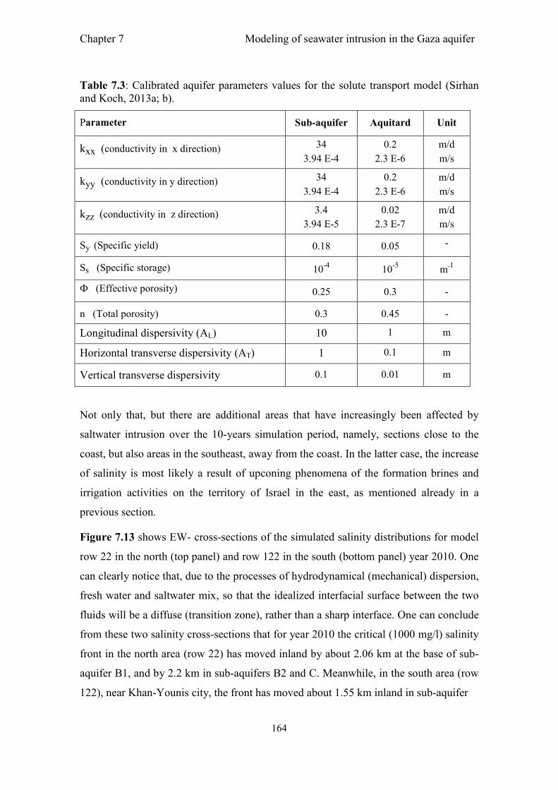
Chapter 7 Modeling of seawater intrusion in the Gaza aquifer
164
Table 7.3: Calibrated aquifer parameters values for the solute transport model (Sirhan and Koch, 2013a; b).
Parameter Sub-aquifer Aquitard Unit
kxx (conductivity in x direction) 34
3.94 E-4
0.2
2.3 E-6
m/d
m/s
kyy (conductivity in y direction) 34
3.94 E-4
0.2
2.3 E-6
m/d
m/s
kzz (conductivity in z direction) 3.4
3.94 E-5
0.02
2.3 E-7
m/d
m/s
Sy (Specific yield) 0.18 0.05 -
Ss (Specific storage) 10-4
10-5
m-1
Ф (Effective porosity) 0.25 0.3 -
n (Total porosity) 0.3 0.45 -
Longitudinal dispersivity (AL) 10 1 m
Horizontal transverse dispersivity (AT) 1 0.1 m
Vertical transverse dispersivity 0.1 0.01 m
Not only that, but there are additional areas that have increasingly been affected by
saltwater intrusion over the 10-years simulation period, namely, sections close to the
coast, but also areas in the southeast, away from the coast. In the latter case, the increase
of salinity is most likely a result of upconing phenomena of the formation brines and
irrigation activities on the territory of Israel in the east, as mentioned already in a
previous section.
Figure 7.13 shows EW- cross-sections of the simulated salinity distributions for model
row 22 in the north (top panel) and row 122 in the south (bottom panel) year 2010. One
can clearly notice that, due to the processes of hydrodynamical (mechanical) dispersion,
fresh water and saltwater mix, so that the idealized interfacial surface between the two
fluids will be a diffuse (transition zone), rather than a sharp interface. One can conclude
from these two salinity cross-sections that for year 2010 the critical (1000 mg/l) salinity
front in the north area (row 22) has moved inland by about 2.06 km at the base of sub-
aquifer B1, and by 2.2 km in sub-aquifers B2 and C. Meanwhile, in the south area (row
122), near Khan-Younis city, the front has moved about 1.55 km inland in sub-aquifer

Chapter 7 Modeling of seawater intrusion in the Gaza aquifer
165
Figure 7.11: Observed and calculated saline concentrations at wells D67 and E142 (north Gaza) and well L27 (south Gaza), for calibration and validation periods.
0
40
80
120
160
200
2001 2002 2003 2004 2005 2006 2007 2008 2009 2010
Ch
lori
de
con
cen
tra
tio
n (
mg
/l)
Year
Chloride concentration-time series
D67 (Observed)D67 (Calculated)
Calibrated Validated
0
200
400
600
800
1000
1200
1400
1600
2001 2002 2003 2004 2005 2006 2007 2008 2009 2010
Ch
lori
de
con
cen
trat
ion
(m
g/l)
Year
Chloride concentration-time series
E142 (Observed)E142 (Calculated)
Calibrated Validated
500
600
700
800
900
2001 2002 2003 2004 2005 2006 2007 2008 2009 2010
Ch
lor i
de
con
cen
trat
ion
(m
g/l)
Year
Chloride concentration-time series
L127 (Observed)L127 (Calculated)
ValidatedCalibrated

Chapter 7 Modeling of seawater intrusion in the Gaza aquifer
166
(a) (b) (c)
Figure 7.12: Simulated salinity distribution at the bottom of the aquifer for years 2000 (a), 2005 (b) and 2010 (c).
B1, and by 2.0 km in sub-aquifers B2 and C. Moreover, due to the presence of aquitard
(clay) layers, which separate the sub-aquifers, where the latter have higher hydraulic
conductivity and dispersivity values than the former, the simulation results show the
development and propagation of saltwater fingers.

Chapter 7 Modeling of seawater intrusion in the Gaza aquifer
167
Figure 7.13: EW- cross-sections of year 2010-simulated salinity distributions for model row 22 in the north (top) and row 122 in the south (bottom).
7.6. Evolution of seawater intrusion over the 2000-2010 decade
For various simulation times graphs of the salinity as a function of the distance from the
coastline, i.e. in west to east direction, within a particular sub-aquifer have been
produced from the transient 3D-salinity distributions. Figure 7.14 shows these graphs
for sub-aquifer C in a section south of Khan-Younis city for years 2000, 2005 and 2010.

Chapter 7 Modeling of seawater intrusion in the Gaza aquifer
168
Figure 7.14: Extensions of inland moving seawater intrusion in sub- aquifer C for different times.
For the illustration purposes the critical 1000 mg/l salinity line is shown as an additional
horizontal line. The intersection of the latter with the concentration line gives then the
location of that critical interface point for the different times mentioned. From the figure
one can deduce that this 1000 mg/l concentration point has moved from a distance of 1
km from the coast in 2000 to 1.5 km in 2005 and 2.05 km in 2010.
Moreover, Figure 7.15 shows the locations of fresh/saltwater interface (defined by the
1000 mg/l TDS salinity isoline) in sub-aquifer C along an EW-cross-section in the north
of Gaza for simulation years 2000, 2005 and 2010. One can conclude from the positions
of these isolines that there is a gradual inland invasion of seawater with time. Since it
can certainly be assumed that the inland movement of this saltwater intrusion front has
gone unabatedly up-to-date and will continue to do so in the near future, without
installment of any pre-emptive aquifer management strategies, endeavours to forestall
imminent future water deficiencies as well as quality (salinization) problems and to
restore and/or maintain the sustainability of the Gaza groundwater system for now and
the near future, are becoming extremely urgent. Therefore, predictive simulations of
flow and transport in the Gaza coastal aquifer for the near future will be carried in the
following chapter, assuming different future scenarios, including (1) a "do-nothing"
strategy and (2) the application of various groundwater management strategies for
artificial recharge of the Gaza aquifer.
0
5000
10000
15000
20000
25000
0 500 1000 1500 2000 2500 3000 3500
(TD
S)
mg
/l
Distance from coastline (m)
2000200520101000 mg/l

Chapter 7 Modeling of seawater intrusion in the Gaza aquifer
169
Figure 7.15: Locations of inland moving fresh/saltwater interface (1000 mg/l TDS) in sub- aquifer C along an EW-cross-section in the north for years 2000, 2005 and 2010.
7.7. Sensitivity analysis of hydrodynamic dispersion
A model sensitivity analysis has also been carried out, in order to assess the effects of
the hydrodynamic dispersion coefficient D on the behavior of the density-dependent
solute transport. Such a sensitivity analysis is the more important, as the dispersivity is
usually not known in real aquifer and, as discussed in Section 7.2, depends, in
particular, on the field scale.
In this sensitivity analysis of the hydrodynamic dispersion, simulations with different
dispersivity values have been executed, wherefore the calibrated, reference dispersivity
value, AL = 10 m has been multiplied by factors 0.2, 0.5, and 2, and the ratio of the
longitudinal to the transversal dispersivity has been kept as indicated in Table 7.3.
The salt concentrations simulated by the SEAWAT-variable-density model for year
2010 using these different longitudinal dispersivities are illustrated in the three panels of
Figure 7.16. One may observed from this figure that the simulated movement of the
seawater intrusion front is rather sensitive to the dispersivity value assumed, such that
for a larger longitudinal dispersivity, the fresh/saltwater interface, defined by the critical

Chapter 7 Modeling of seawater intrusion in the Gaza aquifer
170
Figure 7.16: SEAWAT-simulated saline concentrations along an EW-cross-section in the north for year 2010 for three different values of the longitudinal dispersivity AL, namely, 0.2 (top), 0.5 (middle) and 2 (bottom).

Chapter 7 Modeling of seawater intrusion in the Gaza aquifer
171
salinity isoline of 1000 mg/l TDS, has been moving further inland. This is a somewhat
to-be- expected result, as a larger longitudinal dispersivity leads to a broadening of the
solute mixing front, so that the low-concentration head of the advancing front arrives
earlier than is the case for a more localized, less dispersive concentration front.

Chapter 8 Integrated Water Resources Management
172
Chapter 8 : Numerical Investigation of the Prospects of Integrated Water Resources Management in the Gaza Strip
8.1. Introduction and overview
The ongoing depletion of the coastal aquifer in the Gaza strip due to overexploitation
has led to a significant decline of the groundwater levels, excessive reductions in yields,
and many groundwater wells even going dry. Some of these wells had already to be shut
down, due to an increase of the groundwater salinity above the WHO- 250 mg/l
drinking standard limit. This significant deterioration of the groundwater quality all
across the Gaza strip indicates that, last but not least, owing to the decline of the
groundwater levels, salt water intrusion from the Mediterranean has become an
imminent problem which requires a long-term remediative solution.
Nowadays, because of the disastrous groundwater situation in the Gaza region, there is
an urgent need for any action which can restore or, at least, maintain the sustainability
of the Gaza groundwater system for now and, more so, for the near future. In fact,
proper aquifer management may not prevent seawater intrusion, but may only control it.
Once the groundwater is contaminated by saline water, it is difficult to bring it back to
its original quality, but, at least, one may be able to control the further deterioration of
the groundwater quality by seawater intrusion through specific aquifer management
strategies.
With these premises, the ultimate objective of the present thesis work and what is the
focus of this chapter, is a numerical feasibility study of the, hopefully positive, effects
of artificial recharge, planned in the Gaza strip for some time, on the restoration of the
groundwater levels and on the control of the seawater intrusion on the regional scale
under numerous management scenarios schemes within the target period 2011-2040.
This will be done by using the density-dependent flow and transport model SEAWAT.
More specifically, the SEAWAT-model, as calibrated in the previous chapter, is
employed here to simulate the effects of various near-future groundwater management
strategies on the groundwater quantity and quality of the Gaza aquifer system, whereby

Chapter 8 Integrated Water Resources Management
173
the emphasis will be on the development of particular management policies which may
be able to prevent future aquifer overdraft, which is at the very origin of the increasing
seawater intrusion. This is tantamount to the investigation of the long-term safe, or more
precisely, the sustainable yield (Miles and Chambet, 1995; Maimone, 2004) of the Gaza
aquifer.
In addition, new aquifer management scenarios that have been proposed to increase this
yield and to also control the seawater intrusion, namely, artificial recharge from
wastewater, will be investigated numerically in this chapter for their effectiveness to
achieve these goals.
Indeed, the Palestinian Water Authority (PWA) has already considered the
implementation of a strategic plan for aquifer system recovery (ASR), wherefore
artificial recharge by reclaimed wastewater is one of the most promising options for the
Gaza coastal area, where land is scarce. In fact, artificial groundwater recharge has
become a proven method in recent decades for the conservation of groundwater
resources (Merritt, 1985; Ishaq and Khan, 1997; Bouwer and Rice, 2001; Bouwer,
2002; Reese, 2002) and to maintain a positive condition for aquifer, in terms of both
water quantity and quality. In the future, artificial recharge is expected to become
increasingly necessary, as growing populations require more water, so that more storage
of water is needed to prevent shortages.
8.2. The Gaza emergency technical assistance programme (GETAP)
The Palestinian Water Authority (PWA) has adopted a strategic plan, the so-called Gaza
emergency technical assistance programme (GETAP), for the management of the future
water demand in the Gaza strip and for studies of the feasibility of numerous options
for the supply of water for Gaza, taking into account the political, technical and
economic considerations for each option (Figure 8.1). This strategic plan outlines the
directions for the proposed options under question to be taken, to achieve the goals. A
comparative analysis is conducted after evaluation of each option, with the aim of
identifying a selected set of options which are deemed most feasible over the short,
medium and long term (PWA, 2011).

Chapter 8 Integrated Water Resources Management
174
As indicated in Figure 8.1, the initial screening process in GETAP utilizes four
relatively simple criteria:
Political: Is the option politically acceptable in the current context?
Technical: Is the option technically feasible?
Social: Is the option socially acceptable?
Economic: Is the option affordable, with an acceptable cost-benefit ratio?
Based on these four criteria, GETAP has carried out a comparative study of options
(CSO) which encompasses the following management options (with the first one, option
A, not really included), also shown in Figure 8.2:
Option A: Continuation of the status quo (not part of CSO)
Over the past fifteen years after the establishment of the Palestinian Authority (PA), the
status quo in terms of the general water, wastewater, and environmental situation in the
Gaza strip has been extensively documented by the Palestinian water authority (PWA).
PWA has attempted to identify the consequences of the ´´do nothing option´´, where the
situation is becoming gradually worse, due to continuous overexploitation without
sustainable management, which will accelerate the decline of the groundwater table and,
consequently, also saltwater intrusion over time, resulting in a reduction of fresh
groundwater resources in the Gaza coastal aquifer.
Therefore, additional options to be completed as part of the comparative study of
options (CSO) have been considered:
• Assess the effects that variations in the rate of groundwater abstraction could have on
water availability over the specified 30-year duration period, while taking into
consideration other water supply options.
• Examine other technical options with regard to their feasibility under the present and
future political-, security-, and economic constraints.
More specifically, the five CSO- options, as shown in Figure 8.2, are then

Chapter 8 Integrated Water Resources Management
175
Figure 8.1: Screening criteria used in the development of the CSO-G strategy (PWA, 2011).
Option B: Water demand management
Because of the overall limited water resources in the region, demand management
measures, with the requirement of reducing the utilization of fresh water in both
domestic and agricultural sectors have been incorporated, wherever appropriate (Figure
8.2), including the following:

Chapter 8 Integrated Water Resources Management
176
Figure 8.2: Available options in the status quo at GETAP, and their grouping in related types of interventions (PWA, 2011).
• Reducing system losses, such as those occurring through leakage in water distribution
networks or other forms of "unaccounted for water" (UfW).
• Reusing treated wastewater in the agricultural sector, hence, reducing the sectorial
demand for higher-quality fresh water resources.
• Controlling the demand in the agricultural sector by a variety of means, which may
include alterations in the permitted irrigation timings, changes of crop patterns, and
other types of interventions.

Chapter 8 Integrated Water Resources Management
177
Option C: Potential for wastewater reuse
It consists essentially in the use of alternative water recourses, such as treated
wastewater with an effluent that meets the standards guideline for wastewater reuse,
taking into consideration the quality of the treated effluent and treatment methods, since
any reuse will not be successful at a significant scale, if the wastewater effluent is not of
acceptable quality. .
As shown in Figure 8.2, the CSO includes additional sub-options D, E, and F and
option G of which, although they are not of relevance in the present thesis, should be
mentioned:
Option D: National (within Palestine) transfer of water
Option E: Transfer of water from Israel
Option F: Transfer of water to the Gaza strip from Turkey
As a matter of fact, these three sub-options D, E, and F include the transfer of external
water to Gaza from Palestine (West Bank), Israel or Turkey, respectively. The viability
of these options is still a function of whether a permanent status agreement is reached
between the Palestinian Liberation Organization (PLO) and the Government of Israel
(GOI) over the specified 30 years period. Actually, the transfer of water has been been a
routine matter of discussion in the past between the Palestinian National Authority
(PNA) and the Government of Israel (GOI). Politics and security are the main two
issues that have prevented these options to be realized, in addition to the blockade of
Gaza at the present time. Since the past GOI had failed to meet its commitments under
the Oslo II Agreement (Oslo II, 1995), where it was agreed upon that a small water
amount of 5 MCM/year should be provided, free of charge, to the Gaza strip from the
existing Israeli water system or , in the future, from Israel desalination plants.
Not only that, but the "stealing" of parts of the natural subsurface lateral inflow, which
enters into the Gaza aquifer from the Israeli eastern side (see previous chapters), by
pumping wells close to the Gaza-Israeli border has been considered as a reason for the
ongoing depletion of the coastal aquifer underneath Gaza.

Chapter 8 Integrated Water Resources Management
178
Even more so, technical and economical considerations forestall the use of the sub-
options D, E and F. For all of these reasons, these options are no longer applicable in
the GETAP CSO plan and, thus, cannot be used to solve the existing water crises in the
Gaza strip, which means that only options C or G (or both) should be further
investigated.
Option G: Use of seawater desalination
GETAP has proposed two stages for using seawater desalination in the Gaza strip:
Short term low-volume (STLV): STLV has been selected for providing relatively small
volumes of high quality desalinized sea water for potable use. It is estimated that a
quantity of about 10-13 MCM of desalinized seawater can be produced for domestic use
in the time period 2012-2015, before the regional desalination plants can be
implemented in 2016.
Long term high-volume (LTHV): LTHV regional desalination is planned to avoid the
further aquifer deterioration in the long term. To that avail, two regional desalination
plants have been recommended, with a total capacity of about 129 MCM/year by 2035;
the first will be located in middle Gaza and the second in southern Gaza. On this basis,
the estimated earliest possible time for the first regional desalination facility to be
commissioned would be in early 2016 and the second one in 2025. The United States
Agency for International Development (USAID) has granted resources to the PNA for
designing, construction and supervising these reverse osmosis (RO) Gaza seawater
desalination plants.
In the remainder of this chapter study the CSO-options A (do nothing) and the most viable
option C (wastewater reuse for artificial groundwater recharge) will be numerically
investigated by implementing appropriate aquifer management scenarios into the
SEAWAT model.
8.3. Description of groundwater resources management scenarios
Whereas in the previous chapter, the baseline MODFLOW and SEAWAT- numerical
model have been used to investigate such factors as water balance, recharge, extraction,

Chapter 8 Integrated Water Resources Management
179
seasonal variability and salinity distribution under steady-state and transient conditions
between in the period 2001-2010, now the predictive SEAWAT-model will be applied
to simulate future changes in groundwater levels and salinities, up to year 2040 (the
target time of the GETAP CSO plan). This will be done under two extreme future
groundwater management schemes.
In the first, pessimistic scenario, it is assumed that pumping from the aquifer continues
to increase in the near future, to meet the rising municipal water demand, as well as the
extended agricultural activities, and there is not further recharge to the aquifer than what
is provided by natural precipitation. That means essentially, as possible climate change
effects in the region are discarded, the overall annual natural recharge to the Gaza
coastal aquifer will be most likely lower during the time-horizon considered, as a result
of ongoing urbanization and subsequent surface sealing.
The second, optimistic scenario assumes that treated surficial wastewater can be used as
a source of additional artificial recharge to the aquifer which, in principle, should not
only lead to an increased sustainable yield of the latter, but could, in the best of all
cases, revert even some of the adverse present-day conditions in the aquifer (i.e.
seawater intrusion).
8.4. First scenario: Increased future pumping / no action taken
8.4.1. Setup of the first scenario
The first model scenario is basically a time-extension of the transient simulation carried
out in the previous chapter, but now up to year 2040, assuming that the groundwater
abstraction rate from the aquifer will increase continuously during this time to comply
with the population growth and augmenting agricultural needs, as shown in Figure 8.3,
and that no new water resources, other than natural rainfall infiltration, are available to
recharge the aquifer.

Chapter 8 Integrated Water Resources Management
180
Figure 8.3: Projected future (2010-2040) Gaza aquifer abstraction rates for the first scenario.
More specifically, this projected abstraction rate of Figure 8.3 is the sum of the
increased future domestic water demand, due to population growth, assuming an
average water consumption of 150 l/person/day and of the assumed agricultural
groundwater use. In fact, the latter is estimated to decrease from 80 M m3 in year 2010
to 60 M m3 in year 2040 for two reasons: Firstly, growth of the urban areas which will
invade more agricultural land and, secondly, the groundwater cannot support anymore
the future agriculture activities, as the former will have become too saline to be used for
further crop irrigation (Al-Jamal and Al-Yaqubi, 2001).
8.4.2. Impact on regional groundwater levels
Groundwater head predictions with this external stress scenario are shown in Figure 8.4
for the future years 2020, 2030 and 2040. All simulated head isolines indicate negative
groundwater levels, i.e. the latter are lying below mean sea level, whereby the
depression cones in the north of the Gaza strip go down to -5, -7.6 and -7.6 m (MSL),
for years 2020, 2030 and 2040, respectively, but reach even higher values of -13, -14
and -15 m (MSL), respectively, in the south.
0
50
100
150
200
250
300
350
To
tal
Pu
mp
ing
(M
CM
)
Year
Projection of aquifer pumping

Chapter 8 Integrated Water Resources Management
181
(a) (b)
(c)
Figure 8.4: Predicted heads for 1st scenario for years 2020 (a), 2030 (b) and 2040 (c).
These head results show that the continuously ongoing overexploitation of the Gaza
coastal aquifer will, without sustainable management, result in a very negative impact
on the aquifer, i.e. its situation will be far from sustainable, not only from a quantitative,
but also from a qualitative point of view, as these lower groundwater levels will
accentuate further seawater intrusion, as will be shown in the subsequent sub-section.
From the hydraulic heads, using Darcy's law, 3D- Darcy flow velocities and, after
division by the effective porosity, linear (seepage) velocities for each cell of the finite
difference domain grid are computed. These are shown for year 2040 in two EW- cross-
sections, one along row 26 in the north, and another one along row 126 in the south of
the domain area in the two panels of Figure 8.5.

Chapter 8 Integrated Water Resources Management
182
Figure 8.5: Seepage velocity vectors in an EW-cross-section along row 26 in the north (top) and row 126 in the south of the domain (bottom) for year 2040 for the 1st scenario.
It is clear from this the northern cross-section in the top panel of Figure 8.5 that there is
no discharge of groundwater to the Mediterranean Sea any longer, as the velocity
vectors are directed inland, with an upward-directed component in the direction of the
pre-existing cone of depression, i.e., towards the main well field, inducing sea water
intrusion and a subsequent deterioration of the freshwater quality. This well field, with
its large depression cone, pulls in water also from the eastern side of the domain, with
particularly high velocities there, as the infiltration rate in this part of the domain area
is low, owing to low-permeable soils here (dark/reddish brown).

Chapter 8 Integrated Water Resources Management
183
For the south EW- cross section (bottom panel of Figure 8.5) the situation is somewhat
similar, i.e. the flow velocities indicate the propensity for strong seawater intrusion into
the Gaza aquifer in this southern part of the Gaza strip.
8.4.3. Impact on salinity distribution
In addition to the future groundwater heads, the calibrated SEAWAT - model provides
information on the evolution of the groundwater salinity of the Gaza aquifer, due to
seawater intrusion.
From a qualitative point of view, the results obtained with this first management
scenario, i.e. a continuation of the status quo with ongoing overexploitation of the
aquifer without sustainable management, indicate a very negative impact on the aquifer,
since the pre-development salinity interface along the coastal line will continue to move
inward in the coming thirty years. This is clearly illustrated in Figure 8.6 which shows
the predicted salinity distributions of sub-aquifer C with external stress scenario for the
future years of 2020, 2030 and 2040.
One may notice from Figure 8.6 that the areas most affected by seawater intrusion are
located in the south and north of Gaza, where up to year 2040 the salt-fresh water
interface has moved inland towards the freshwater zone, with an average rate of 68 m/y,
57 m/y and 96 m/y in the north, middle and south areas, respectively, which means that
fresh water flushing into the Mediterranean sea will have decreased significantly by that
time. Thus, compared with the baseline saltwater intrusion situation for year 2010, the
salinity by year 2040 will have increased along the pre-development interface and the
latter will have moved by an additional 2, 1.7 and 2.9 km, which corresponds to a 30%,
29% and 42% of increase salinity extent in the north, middle and south areas,
respectively.
A more quantitative assessment of the aquifer’s water budget illustrate that the amount
of seawater intrusion into the Gaza aquifer is 86, 100, and 109 M m3 in years 2020,
2030 and 2040, respectively, compared with only 71 M m3 for the baseline year 2010.
This corresponds to a 35% increase of the amount of the intrusion of saline water into
the coastal aquifer by year 2040, compare with the present-day situation.

Chapter 8 Integrated Water Resources Management
184
(a) (b) (c)
Figure 8.6: Salinities for 1st scenario for years 2020 (a), 2030 (b) and 2040 (c).
In conclusion, both the future head and salinity results of this first do-nothing
SEAWAT- management scenario model clearly indicate that, without any remediative
near-future actions taken, there will be an ongoing future deterioration of the
groundwater quality over the whole Gaza strip, due to accelerated salt water intrusion
from the Mediterranean sea.

Chapter 8 Integrated Water Resources Management
185
8.5. Artificial recharge systems
Artificial recharge into the aquifer system has been widely used for groundwater
remediation. In fact, underground storage via artificial recharge is a proven method for
the conservation of groundwater resources, as it has the advantage of essentially reduce
the evaporation from the aquifer to zero. The main objective of artificial recharge
consists in the restoration of the groundwater levels, and, by creating a hydraulic
gradient towards the sea, controlling or reverting seawater intrusion. In fact, artificial
recharge of groundwater is expected to play a significant important role in water reuse
through the soil aquifer treatment (SAT) or geo-purification of the effluent, which gives
an additional treatment by seepage through the porous media of the aquifer (Ishaq and
Khan, 1997).
Noteworthy is still here that the reuse of treated wastewater for artificial aquifer
recharge depends fundamentally on the completion of these high-quality wastewater
treatment facilities to avoid clogging of the recharge system by inorganic (clay and silt)
and organic (algae, sludge) suspended solids that accumulate on the infiltration surface
(Fitzpatrick, 1986). This includes also, the removal of the suspended solid (SS), the
reduction of the biological oxygen demand (BOD), the chemical oxygen demand
(COD), and the removal of nutrients such as nitrogen and phosphorous, and bacteria,
such as F. – Coliform (Aiesh, 2004, citing Zubiller, 2002). All these parameters should
meet the standards quality requirements for wastewater recharge.
Artificial recharge of aquifers can be applied through several systems as described in
the following sub-sections:
8.5.1. Surface infiltration
Surface infiltration systems for artificial recharge can be used in the case when a
sufficiently large area for surface infiltration is available. The most common technique
for this system is the infiltration basin, as shown in Figure 8.7. The water is spread on
the ground to let infiltrate into the soil so that it can move towards the underlying
groundwater. This means, of course, that the recharging water should be of adequate
quality to prevent undue clogging of the system, resulting from depositions,
accumulation of suspended solids and formation of surface algae (Bouwer, 2002).

Chapter 8 Integrated Water Resources Management
186
Figure 8.7: Groundwater recharge using an infiltration basin (Barlow, 2003).
As a matter of fact, the infiltration basins require permeable soil of the storage zone,
which may greatly affect recoverability, so that for a check of the recharge efficacy of
the infiltrated water, it is important to analyze the soil properties of the surficial layers
(Merritt, 1985). Thus, if the latter consist of clay, boreholes through them have to be
drilled to reach the permeable layer, which in some cases means borehole depths of
more than 25 m below the basin surface.
8.5.2. Vertical infiltration systems
Where sufficient permeable soils and/or sufficient land areas surface infiltration system
are not available, groundwater recharge can also be achieved with vertical infiltration
systems, such as trenches or wells in the vadose zone, where the latter must reach the
deeper aquifer layers, as shown in Figure 8.8. Vadose zone wells are also called
recharge shafts or dry wells. Recharge trenches are dug with a backhoe and are typically
less than about 1 m wide and up to about 5 m deep. They are backfilled with coarse
sand or fine gravel, whereby the function of the upper parts of the system act as
drainage for the perched groundwater, meanwhile the lower parts are used for
recharging the aquifer through infiltration (Bouwer, 2002). One of the advantages of
such a system is that the filtered water can get an additional treatment by soil aquifer

Chapter 8 Integrated Water Resources Management
187
Figure 8.8: Sections showing surface infiltration systems with restricting layer (hatched) and perched groundwater drainage to unconfined aquifer with trench (left), vadose-zone well (center) and aquifer well (right) (Bouwer, 2002).
Figure 8.9: Recharge (A) and discharge (B) phases for an idealized aquifer storage and recover well in south Florida (Barlow, 2003).

Chapter 8 Integrated Water Resources Management
188
treatment (SAT) process through the porous soil, therefore avoiding to a large extent the
clogging problem.
Direct recharge or injections wells are used where permeable soils and/or sufficient land
area of surface infiltration are not available, where vadose zones are not suitable for
trenches or wells, and where aquifers are deep and/or confined, as shown in Figure 8.9.
Theoretically, recharge of freshwater into the saline water aquifer creates a radial zone
of mixing (the transition zone) around the well that separates the native saline water
from the injected freshwater (Reese, 2002). In reality, the shapes of the injected
freshwater zone and of the mixing zone are highly dependent on the geology of the
injection zone, such as the permeability of the injection zone, the aquifer thickness and
the surrounding hydraulic gradient. Mixing between the injected freshwater and the
native saline water can reduce the amount of freshwater that is recovered during the
withdrawal phase (Barlow, 2003).
8.6. Second scenario with different cases of artificial recharge from treated
wastewater
In this second management scenario which will be investigated in three different
variants, treated surficial wastewater will be used as a source of artificial recharge to the
aquifer, to maintain or restore positive conditions for the groundwater, both
quantitatively (water balance) and qualitatively (salinity) and, if possible, to revert the
adverse situation in the near future.
8.6.1. Proposed wastewater artificial recharge design
It is assumed that the wastewater for recharge comes the effluent of the four main
wastewater treatment plants (WWTP) in the Gaza strip (see Figure 8.10). In addition to
these existing plants, there are plans to build three new large-scale WWTP in several
stages, starting with a primary treatment plant plus short sea outfalls, supplemented later
by a tertiary treatment plant plus a reuse of the treated wastewater (see Table 8.1), in
order to minimize the risks associated with the release of untreated wastewater into the
environment (PWA, 2011). In the long-term, these WWTP will also provide additional

Chapter 8 Integrated Water Resources Management
189
quantities of water for re-use in agriculture and for artificial recharge. Figure 8.11
shows the future wastewater production in the Gaza strip up to the year 2040.
Table 8.1: Proposed WWTPs for Gaza (PWA, 2011).
Treatment
plant
Status Year Capacity
(MCM/yr)
Funding
agency
Costs
(million S$)
Technology
Northern
Gaza
Under
construction
2015-phase 1
2020-phase 2
12.8
22
World
Bank
50 Plug
flow/Complete
mixing
Central
Gaza
Detailed
design
2025 72.7 Germany
(KfW)
70 Oxidation
ditch
Southern
Gaza
Detailed
design
2025 16 Japan 35 Oxidation
ditch
Total 123.5 155
8.6.2. Numerical implementations of the artificial recharge system
The proposed artificial recharge system has been implemented numerically in
SEAWAT in three different variants, or cases, that differ by the locations and
extensions of the well fields where the treated wastewater will be injected. The reason
for generating these three configurations is to come up with the most appropriate
locations within the domain environment for the recharge, in order to create a hydraulic
gradient toward the sea and to achieve a quasi-stabilization of a minimum water level
(MSL=0) and, also, to revert or, at least, to control the seawater intrusion in the aquifer
in the long run.
In all three variants of the artificial recharge scenario, the injection of the wastewater is
assumed to start in 2015 and continues until the end of the simulation period in 2040,
with the hope to achieve a quasi-stabilization of the groundwater heads at the minimum
water level of 0 m above MSL by that time.

Chapter 8 Integrated Water Resources Management
190
Figure 8.10: Existing and Planned WWTPs in Gaza (PWA, 2011).
Figure 8.11: Projection of future wastewater production in the Gaza strip.
0
20
40
60
80
100
120
140
160
2010 2015 2020 2025 2030 2035 2040
Was
t wat
er P
rod
uct
ion
(MC
M)
Year
Proposed WWTP
Existing WWTP
Chapter 8 Integrated Water Resources Management
191
8.6.3. First recharge scenario
In this first (and also the second) recharge case it is assumed that the applied
groundwater recharge follows roughly the available production of treated wastewater
(see Figure 8.11), i.e., it starts from 50 M m3 in year 2015, increases gradually by an
increment of 2 M m3 per year, to finally reach 100 M m3 in year 2040.
The particular feature of this first case is that the artificial recharge scenario is applied
in the form of two agglomerations or fields of injection wells, located more or less
above the two groundwater head depression cones, that have already been established
for year 2010 in the south and north of the Gaza strip, respectively (see Figure 6.15).
The locations and extensions of these two well-fields are shown in Figure 8.12. About
50 injection wells have been used in each of the two well-fields and are supposed to
receive the effluent of the treated surficial wastewater.
8.6.3.1. Impact on regional groundwater levels
For this first case of the second groundwater management scenario, the simulation
results hints of some success for achieving the objective intended, namely, the aquifer
remediation in the long-term and the restoration of the groundwater levels. In fact,
Figure 8.13 demonstrates that there is a gradual aquifer recovery with time, as the zones
of the cones of depression in the north and the south of the Gaza strip are disappearing
more and more for years 2020, 2030 and 2040. Not only that, but the artificial recharge
will have induced a groundwater mound in these areas of up to 2 - 4 m above MSL by
the end of the simulation period in 2040, i.e. the depression cones have converted to
ascension cones. These groundwater mounds will, necessarily, lead to a hydraulic
gradient from its summit to the coastline which, in turn, will drive groundwater flow in
this direction. This can be clearly seen from Figure 8.14 which shows the flow velocity
vectors in two EW-cross- section in the north and south of the Gaza strip at the end of
year 2040. In contrast to the situation of the first management scenario (no artificial
recharge) (see Figure 8.5), the flow direction is now reverted in this case scenario.
The transient evolutions of the groundwater heads, i.e. the development of the
groundwater mound in the centers of the north and south pre-existing depressions,

Chapter 8 Integrated Water Resources Management
192
Figure 8.12: Locations of injection well groups for the 2nd (1st case) scenario.
relative to their 2015 values, are presented in the two panels of Figure 8.15. It is clear
from this figure that the groundwater is maintained by 7 m and 13 m in the critical area
of pre-existing depression-cones in the north and south, respectively up to year 2040.
Comparing these values with those existing at the end of the transient simulation time
period in 2010 (see Figure 6.15) one may note that the break-even time when the
depression-cones in the north and south have disappeared is around 2025 and 2030,
after which time mounding above sea-level will occur.
Moreover, a comparison of groundwater heads for the two scenarios is shown in the
EW- cross-sections of the 2040 simulated groundwater heads through the two existing
depression cones in the north and the south of the study area and for the two
management scenarios discussed in Figure 8.16. Thus, the curves for each of the two
scenarios clearly shows the positive effect of the first case of the 2nd (artificial recharge)
scenario, as the groundwater levels rise more or less steadily with increasing distance
from the coastline, unlike for the 1st scenarios, where the head decreases away from the

Chapter 8 Integrated Water Resources Management
193
(a)
(b)
(c)
Figure 8.13: Heads for 2nd scenario (1st case) for years 2020 (a), 2030 (b) and 2040 (c).
coastline, until the center of the cone of depression is met, after which on it increases
again when going towards the eastern border of the model domain.
A more quantitative assessment shows that, the additional water by the artificial
recharge contributes balances of the aquifer water budget by 81 %.
8.6.3.2. Impact on salinity distribution
The qualitative picture for this recharge scenario is provided in Figure 8.17 which
indicates that there is a slight continuous decrease of the groundwater salinity in the pre-
development interface along the coastal shore, until the end of simulation period in year
2040. Thus, Figure 8.17 illustrates that by year 2040, compared with the "do-nothing"
first scenario (see Figure 8.6), the critical (1000 mg/l) salinity front at the base of sub-

Chapter 8 Integrated Water Resources Management
194
Figure 8.14: Seepage velocities in EW-cross-section along row 26 in the north (top) and row 126 in the south of the domain (bottom) in 2040 for 2nd (1st case) scenario.
aquifer C has moved backwards towards the sea by about 1.2, 0.1 and 1.8 km, which
corresponds to a 18%, 2% and 26% of reducing the saltwater-polluted sections in the
north, middle, and south areas, respectively, up to the end of simulation period in 2040.

Chapter 8 Integrated Water Resources Management
195
Figure 8.15: Growth of the groundwater mound at the center of the north (top) and the south (bottom) pre-existing depressions cones, relative to the 2015-minimum.
0
1
2
3
4
5
6
7
8
9
2015 2020 2025 2030 2035 2040
Mo
un
d h
eig
ht
(m)
Year
Mound growth
0
2
4
6
8
10
12
14
16
2015 2020 2025 2030 2035 2040
Mou
nd
hei
ght
(m)
Year
Mound growth

Chapter 8 Integrated Water Resources Management
196
Figure 8.16: Groundwater water levels along two EW-cross section in the north (top) and in the south (bottom) for year 2040 for the two groundwater management scenarios (1st : without; 2nd (first case) : with artificial recharge).
-18
-14
-10
-6
-2
2
6
10
0 1000 2000 3000 4000 5000 6000 7000 8000 9000
Wa
ter
lev
el (
m)
Distance from the sea
1st scenario2nd (case 1)scenario
Cone of depression
Mound height
-18
-14
-10
-6
-2
2
6
10
0 1500 3000 4500 6000 7500 9000 10500 12000
Wat
e r le
vel
(m)
Distance from the sea
1st scenario
2nd (case 1)scenario
Cone of depression
Mound height

Chapter 8 Integrated Water Resources Management
197
(a) (b) (c)
Figure 8.17: Salinity for 2nd scenario (1st case) for years 2020 (a), 2030 (b) and 2040 (c).
8.6.4. Second recharge scenario
In the second case of the second (recharge) scenario, the artificial recharge is
implemented through a series of injection wells located upstream of the highly
contaminated zone (salinity > 1000 mg/l TDS) and along the seawater intrusion front,
parallel to the coastline (Figure 8.18). The injection rates used in SEAWAT in this
scenario case follow approximately the assumed production of treated wastewater
during the simulation period (see Figure 8.11).

Chapter 8 Integrated Water Resources Management
198
Figure 8.18: Locations of injection wells for the 2nd (2nd case) scenario.
8.6.4.1. Impact on regional groundwater levels
The simulation results for this groundwater management scenario reveal that there is
some success for aquifer remediation in the long-term, namely, a partial restoration of
the groundwater levels (Figure 8.19). Comparing these hydraulic head- results with
those obtained with the first scenario (Figure 8.4), one may notice that, although there
is also in the present case only a partial aquifer recovery, the groundwater levels
remediated by 3 and 6 m, in the two north and south depression-cones, respectively, by
year 2040, this means that at least in these two highly-stressed zones the Gaza aquifer
continues to be overexploited by increased pumping in the long run. Meanwhile the
groundwater levels in the middle of the model area have reached MSL by year 2020 and
continue to rise steadily, going up to 2 m above MSL, until the end of the simulation
period in year 2040, indicating a restoration of the aquifer in that part of Gaza.
80000 85000 90000 95000 100000 105000
75000
80000
85000
90000
95000
100000
105000
110000
0 5000 10000 15000
Injection wells

Chapter 8 Integrated Water Resources Management
199
(a) (b)
(c)
Figure 8.19: Heads for 2nd scenario (2nd case) for years 2020 (a), 2030 (b) and 2040 (c).
Another corroboration of these positive results can also be gained from Figure 8.20
which shows the flow velocity vectors in an EW-cross- section in the middle of the
Gaza strip at the end of year 2040. In contrast to the situation of the first management
scenario (no artificial recharge), the flow direction is now reverted in this case,
particularly, at the western side of the model along the coastal shore, i.e. flushing of
groundwater into the sea is occurring now, as a result of the artificial recharge.
Moreover, in the eastern area, behind the series of injection wells located along the
seawater intrusion front, and, owing to the fact that the infiltration rate in this part of the
domain area is low, as the soils there are rather impermeable (dark/reddish brown and
loessal sandy soil), the velocity vectors are directed inland, with an upward-directed
component.

Chapter 8 Integrated Water Resources Management
200
Figure 8.20: Seepage velocity vectors in an EW-cross-section along row 60 in the middle of the domain area for year 2040 for the 2nd scenario (2nd case).
A more quantitative assessment shows that, the additional water by the artificial
recharge contributes balances of the aquifer water budget by 77 %.
8.6.4.2. Impact on salinity distribution
The qualitative picture obtained for this recharge scenario for the salinity distributions
(Figure 8.21) indicates that there is some success in reducing the groundwater salinity
in the pre-development interface along the coastal shore- which still continued to move
on inward for a while after the beginning of the recharge of reclaimed wastewater into
the aquifer in year 2015- by the end of the simulation period in year 2040. It is obvious
that, the zones of the pre-development interface in the middle area of the model are
disappearing more and more for years 2020, 2030 and 2040. Also, one may notice that
the south area has been affected more by artificial recharge than the north area. Thus
Figure 8.21 shows at the end of year 2040 the critical (1000 mg/l) salinity front at the
base of sub-aquifer C has moved backwards towards the sea by about 0.2, 2.6 and 3.3
km, which comparing with the first (worse) scenario (see Figure 8.6), corresponds to a
4%, 46% and 48% of reducing the saltwater- polluted in the north, middle, and south
areas, respectively up to the end of simulation period in 2040.

Chapter 8 Integrated Water Resources Management
201
(a) (b) (c)
Figure 8.21: Salinity for 2nd scenario (2nd case) for years 2020 (a), 2030 (b) and 2040 (c).
8.6.5. Third recharge case scenario
8.6.5.1. Scenario case description
In the third case of the second (recharge) scenario, the artificial recharge is based on the
implementation of surface infiltration basins for wide-scale reuse of wastewaters as an
aquifer recharge-recovery system, which could be given an additional treatment by soil
aquifer treatment (SAT) or geopurification of the wastewater effluent. The proposed
infiltration basins are planned to be constructed far away from the sea shore, i.e.

Chapter 8 Integrated Water Resources Management
202
adjacent to the proposed wastewater treatment plants in the north and the middle zones
and close to the eastern political border between Gaza and Israel (see Figure 8.22).
As a matter of fact, the agriculture sector is considered the backbone of Gaza economy
and consumes approximately 50 % of total freshwater consumption (PWA, 2010a).
Therefore, in addition to the aquifer recharge-recovery scheme, this intervention could
be used for irrigation purposes in the cultivated areas through recovery wells proposed
around the infiltration basins, and then this can lead to decrease the total abstraction
from the aquifer, which will give positive impacts on aquifer behavior.
In this third case of the second (recharge) management scenario the source of artificial
recharge to the aquifer is assumed to come from the effluent of the planned new two
large-scale wastewater treatment plants (WWTPs) located at the eastern border of the
Gaza strip (see Figure 8.22), which will be built in several stages, whereby the north
and middle wastewater treatment plants are planned to start operation in year 2015 and
2025 respectively. The injection of the treated wastewater is then assumed to start in
2015 in the north, and in 2025 in the middle, whereas the wastewater effluent from the
south plant is not planned for reuse (PWA, 2011). The overall artificial recharge rates
used in this management scenario case follows roughly the available production rate of
the treated wastewater (see Table 8.1).
Thus in the north, the recharge rates start with 13 M m3 in year 2015, increases
gradually by an increment of 1.4 M m3/year until year 2020, after which time the
recharge rate is kept constant up to the end of year 2040. For the middle zone the
recharge will start in 2025, with a rate of 73 M m3/year which is kept constant until the
end of the target period in 2040 (Figure 8.23).
Estimation of the land area needed and the infiltration rates are the most important
aspects for the planning and designing of the infiltration basins system. In this case, the
proposed area of infiltration basin in the north will be about 45,000 m2, with an average
infiltration rate of 1.3 m/d applied between years 2020 and 2040. Meanwhile, the
infiltration basin in the middle will have an area of about 90,000 m2, with an average
infiltration rate of 2.2 m/d applied between years 2025 and 2040.

Chapter 8 Integrated Water Resources Management
203
Figure 8.22: Proposed locations of the infiltration basins sites in the Gaza strip for the 2nd scenario (3rd case) (adapted from PWA, 2011).
Figure 8.23: Recharge rates of the two infiltration basins at north and middle area.
0
10
20
30
40
50
60
70
80
2010 2015 2020 2025 2030 2035 2040
Rec
har
ge r
ate
(MC
M)
Year
Recharge-north
Recharge-middle
Proposed infiltration basins

Chapter 8 Integrated Water Resources Management
204
The infiltration basins of artificial recharge have been numerically modeled by
assigning aerially recharging zones at the specified locations in the model, with
infiltration rates equal to the average artificial recharge rates listed above for the two
recharging basins in the north and the middle sections of the eastern border of Gaza.
8.6.5.2. Impact on regional groundwater levels
For this third case of the second groundwater management (artificial recharge) scenario,
the simulation results for the hydraulic heads are shown in Figure 8.24. One may notice
a continuously ongoing restoration of the aquifer, as the groundwater levels in the
groundwater mound in the north and middle areas of up to 20 m above MSL by the end
of the simulation period in 2040, i.e. the depression cones have converted to ascension
levels are still occurring there. Thus, compared with the heads of the first (no artificial
recharge) scenario (see Figure 8.4), the heads in the vicinity of Khan-Younis city in
south Gaza and the southeastern area have been remediated by 3 m and 5 m,
respectively, by to year 2040.
A more quantitative assessment shows that, the additional water by the artificial
recharge contributes balances of the aquifer water budget by 72 %.
8.6.5.3. Impact on salinity distribution
The simulation results for the salinity of this groundwater recharge scenario
demonstrate that there is also some success in the recovery of the aquifer quality,
sometime after the beginning of the recharge of reclaimed wastewater into the aquifer in
year 2015. Thus, from the salinity distributions of Figure 8.25 it is obvious that the
critical saline area between the coast and the 1000 mg/l TDS isoline of the pre-
development interface, north of Gaza city, in the middle of the model domain is
disappearing more and more for years 2020, 2030 and 2040. Not only that, but the
artificial recharge has also locally diluted the salinity more in the east of the aquifer,
namely, in the north and even more so in some areas in the middle of the Gaza strip.
This is similar to the heads (Figure 8.24), where the middle and Gaza city areas have
been more affected by the artificial recharge than the north area. A more quantitative
analysis of Figure 8.25 illustrates that by year 2040, compared with the "do-nothing"
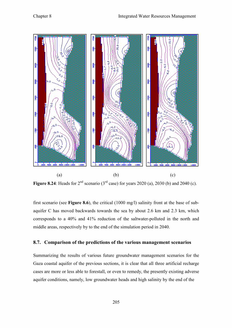
Chapter 8 Integrated Water Resources Management
205
(a)
(b)
(c)
Figure 8.24: Heads for 2nd scenario (3rd case) for years 2020 (a), 2030 (b) and 2040 (c).
first scenario (see Figure 8.6), the critical (1000 mg/l) salinity front at the base of sub-
aquifer C has moved backwards towards the sea by about 2.6 km and 2.3 km, which
corresponds to a 40% and 41% reduction of the saltwater-polluted in the north and
middle areas, respectively by to the end of the simulation period in 2040.
8.7. Comparison of the predictions of the various management scenarios
Summarizing the results of various future groundwater management scenarios for the
Gaza coastal aquifer of the previous sections, it is clear that all three artificial recharge
cases are more or less able to forestall, or even to remedy, the presently existing adverse
aquifer conditions, namely, low groundwater heads and high salinity by the end of the

Chapter 8 Integrated Water Resources Management
206
(a) (b) (c)
Figure 8.25: Salinity for 2nd scenario (3rd case) for years 2020 (a), 2030 (b) and 2040 (c).
target simulation period, year 2040 as shown in Figure 8.26 and 8.27. The positive
effects of this second (recharge) scenario groups become even more striking, when
compared with the first (do-nothing) management scenario which is the most critical
one, as it assumes ever-increasing groundwater extraction in the coming 30 years.
As a matter of fact, the first (do-nothing) scenario illustrate that at the end of the
simulation period, year 2040, the amount of saltwater intrusion into the coastal part of
the aquifer increases by about 35 %, meanwhile the salinity will be increased by 34 %.

Chapter 8 Integrated Water Resources Management
207
In contrast, all three cases of the second (artificial recharge) scenario group can partly
revert the present seawater intrusion. From the water budget point of view, compared
with the first (do nothing) scenario, for year 2040 the additional water to the aquifer by
the artificial recharge reduces the amount of water entering the aquifer by seawater
intrusion by 81%, 77% and 72 %, for the three recharge cases, respectively (Figure
8.28). Moreover, the artificial recharge reduces the saltwater-polluted (salinity) in the
Gaza aquifer by 15%, 32% and 26% for the three cases respectively (Figure 8.29).
Table 8.2 summarizes the water budget components for the four water management
scenarios by the end of the simulation period in year 2040 in a comparative manner.
The estimated hydraulic heads show that the 1st case of the second artificial recharge
scenario is the best option for achieving the aquifer remediation in the long-term in
terms of groundwater levels restoration (see Figure 8.28). Meanwhile, the 2nd case of
the second (artificial recharge) scenario is the best option in term of reducing the
salinity (TDS) in the long-term, while the 3rd case would be the second effective option
in reducing aquifer salinity (see Figure 8.29).
As a matter of fact, the results of the numerical modeling with the artificial recharge
scenarios indicate that there is some success in aquifer recovery that may forestall or
remedy the adverse aquifer conditions, such that the presently existing saltwater
intrusion is partly been reverted by the end of simulation period in year 2040.
Table 8.2: Summary of water budget components for the four water management scenarios by the end of the simulation period in year 2040.
Indicator First scenario
(do nothing)
Second scenario (with artificial recharge)
Case 1 Case 2 Case 3
Seawater intrusion Mm3/year.
109 21 25 31
% Change of seawater intrusion amount.
+ 35% - 81 % - 77 % - 72 %
% Change on salinity distribution.
+ 34 % - 15 % - 32 % - 26 %

Chapter 8 Integrated Water Resources Management
208
(a) (b) (c) (d)
Figure 8.26: Year-2040 head for 1st scenario (a), compared with 2nd scenario of 1st case (b), 2nd case (c) and 3rd case (d).
(a) (b) (c) (d)
Figure 8.27: Year-2040 salinity for 1st scenario (a), compared with 2nd scenario of 1st case (b), 2nd case (c) and 3rd case (d).
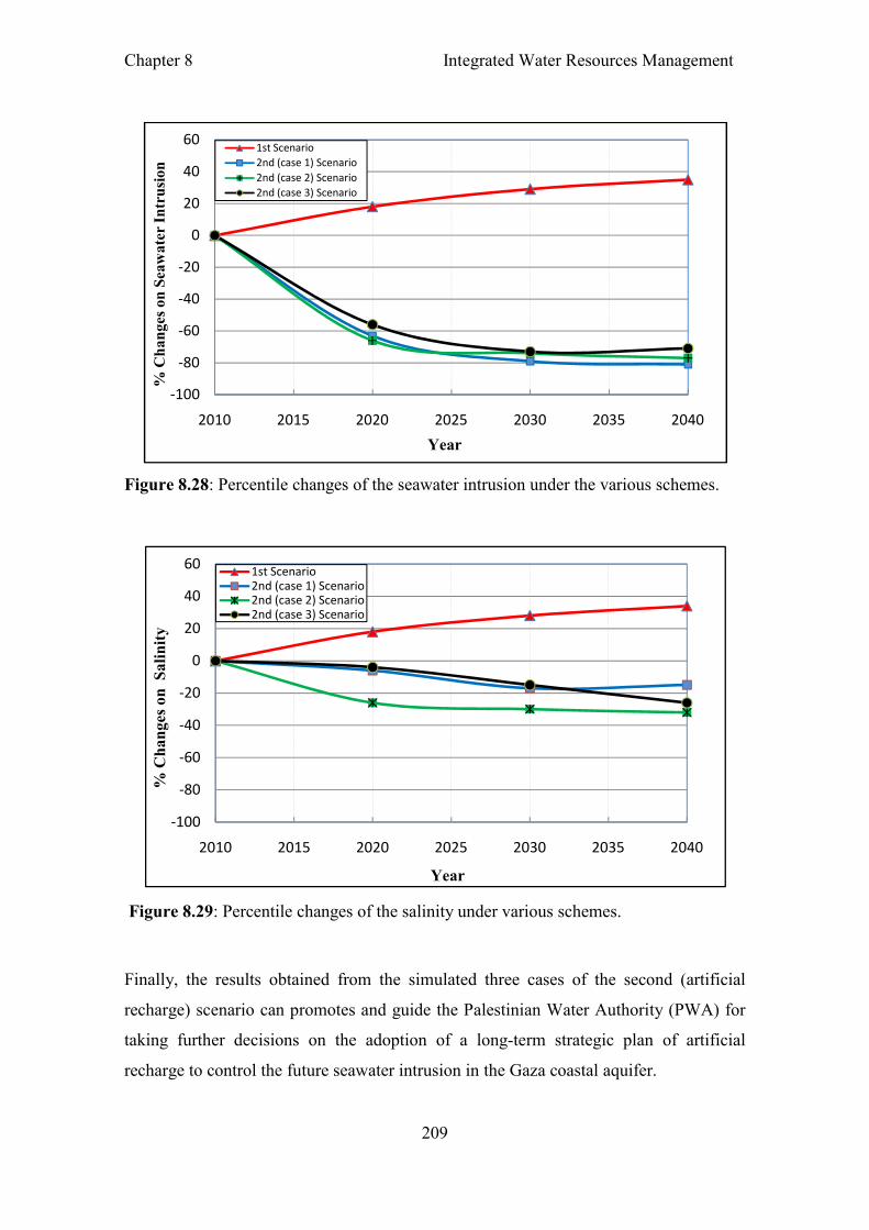
Chapter 8 Integrated Water Resources Management
209
Figure 8.28: Percentile changes of the seawater intrusion under the various schemes.
Figure 8.29: Percentile changes of the salinity under various schemes.
Finally, the results obtained from the simulated three cases of the second (artificial
recharge) scenario can promotes and guide the Palestinian Water Authority (PWA) for
taking further decisions on the adoption of a long-term strategic plan of artificial
recharge to control the future seawater intrusion in the Gaza coastal aquifer.
-100
-80
-60
-40
-20
0
20
40
60
2010 2015 2020 2025 2030 2035 2040
% C
ha
ng
es o
n S
eaw
ate
r In
tru
sio
n
Year
1st Scenario
2nd (case 1) Scenario
2nd (case 2) Scenario
2nd (case 3) Scenario
-100
-80
-60
-40
-20
0
20
40
60
2010 2015 2020 2025 2030 2035 2040
% C
han
ges
on S
alin
ity
Year
1st Scenario2nd (case 1) Scenario2nd (case 2) Scenario2nd (case 3) Scenario
Chapter 9 Conclusions
210
Chapter 9 : Conclusions and Recommendations
9.1. Conclusions
The ongoing depletion of the coastal aquifer in the Gaza strip, due to overexploitation
and, possibly, negative impacts as a result to climate change, has led to a significant
decline of the groundwater levels, excessive reductions in yields, and many
groundwater wells even going dry over the last two decades. Some of these wells had
already to be shut down in recent years, as their measured groundwater salinities
exceeded the WHO- 250 mg/l drinking standard limit. This significant deterioration of
the groundwater quality all across the Gaza strip indicates that salt water intrusion from
the Mediterranean sea, accelerated by the decline of the groundwater levels, has become
an imminent problem.
In light of these imminent groundwater problems in the Gaza aquifer, long-term
remediative solutions are asked for. One way to this, is the application of appropriate
integrated groundwater management strategies for this aquifer, in order to maintain its
sustainability and to forestall future problems. The investigation of the applicability and
feasibility of such management strategies can only be effectuated properly by numerical
groundwater flow and transport modeling. This has been the major theme of the present
thesis research.
As an initial stage of the present study, the empirical model of artificial neural networks
(ANN) has been applied as a new approach and as an attractive tool to study and to
predict groundwater levels, without applying physically-based hydrologic parameters.
This ANN- approach may improve the understanding of complex groundwater system, in
particular, when geological and hydro-geological data on the aquifer, as well as
groundwater data, is partly missing or fraught with errors, so that a deterministic model
is difficult to be set up.
The ANN-technique used here is based on a feed-forward neural network, where the
network is trained using forward propagation of the inputs and backward propagation of

Chapter 9 Conclusions
211
the error, to update the unknown activation weights between the neurons of the different
layers.
The optimal ANN-model for predicting groundwater levels in the Gaza coastal aquifer is
developed in two major steps.
In the first step an initial ANN-model is set up, after numerous trial-and-error tests as a
3-layer MLP network, and using the seven variables: initial groundwater level,
groundwater extraction rate, recharge from rainfall, hydraulic conductivity, distance of a
well from the shoreline, depth to the well screen and the well density across the area, as
input neurons. This initial ANN-model results in a very good agreement between
simulated and observed groundwater levels with a correlation coefficient of R=0.97.
In the subsequent sensitivity analysis the influential model input parameters are
analyzed, by computing the significance of individual variables in the ANN- model. The
results of this sensitivity analysis, using the ranks of the parameter influences, indicate
that the two independent variables, depth to well screen and hydraulic conductivity, are
the least important variables for predicting the groundwater levels and can, thus, be
ignored in the final ANN- model.
In the second step the final ANN-model is set up retaining only the five most influential
input variables. After numerous trials the best final ANN-model is found to be a four
MLP (5:5:30:20:1) network, with two hidden layers between input and output layer. This
final ANN- model is trained, validated and tested successfully, and results in an overall
correlation coefficient of R=0.97 between simulated and observed groundwater levels.
Finally, both response graphs and response surfaces are used to get some more physical
insight into the aquifer system’s behavior, by studying the relationships between
independent and dependent variables. Thus monotonous increases of the final water
levels WLf with the initial water levels WLi and with the groundwater recharge R, but
decreases with the pumping (abstraction) rate are observed, whereas the dependencies of
the former on the distance of the wells to the shore and on the well density are not so
clear.

Chapter 9 Conclusions
212
In contrast, the variations of WLf as a function of the distance of the well to the shore
Dshore and of the well-density Wdens are more complicated, since the corresponding
graphs exhibit some oscillatory, or unstable behavior. Meanwhile, from the response
surface, several statements can be made. Thus it can be seen that the final water levels
WLf are particularly sensitive to the initial water levels WLi and, depending on the
pumping rate Q, also on Dshore, moreover, for high pumping rates Q, the well-density
Wdens has also a strong effect on the final water levels.
The final ANN-model obtained in this way is used as a complement to the subsequently
developed classical (deterministic) groundwater model for the Gaza aquifer, in order to
better understand the influential parameters on the groundwater flow behavior in that
region.
The major part of the present thesis research is then devoted to the application of a
classical (deterministic) groundwater model, with the ultimate purpose to simulate
various future groundwater management scenarios, that may forestall or even remedy
the adverse conditions which presently exist in the Gaza aquifer.
Here the 3D- finite difference, coupled groundwater flow and contaminant transport
model MODFLOW/MT3D/SEAWAT, as implemented in the Visual MODFLOW
software, has been applied for this purpose. This modeling package has been chosen
because of its easy-to-use interface, which has been specifically designed to increase
modeling productivity and to decrease the complexities, typically associated with the
build-up of complex three-dimensional groundwater flow and solute transport models.
The optimal Visual MODFLOW-model for predicting groundwater levels in the Gaza
coastal aquifer is developed in two major steps.
In the first step, steady-state calibrations for year-2000 observed hydraulic heads have
been carried out, by adjusting the hydraulic conductivity/transmissivity, as well as the
amount of natural recharge. A good agreement between simulated and observed
groundwater levels, with a correlation coefficient of R= 0.92, is obtained.
In the second step, the heads of the steady-state calibrated model for year 2000 are used
as initial conditions for the total transient simulation, which are executed over the time

Chapter 9 Conclusions
213
period 2001 -2010. This time span includes a 8-year pure calibration period 2001-2008
and a 2-year validation period 2009-2010. The transient calibration has been carried out
by adjusting the specific yields for the unconfined aquifer layers, and of the specific
storativities for the confined layers, as well as of those for the aquitards. These
parameters have been adjusted manually by a trial and error during these transient
calibration runs, until an acceptable match between observed and calculated heads is
obtained. The average correlation coefficients R, measuring the goodness of the fit of
the simulated to the observed heads for all wells, for the individual months of the
calibration time period 2001-2008 and of the verification period 2009-2010, are R=
0.92 and 0.94, respectively, which indicates that the adjustment of the model to the data
is overall good.
The results of the hydraulic heads, as well as those of the water budget analysis show
also that the physical groundwater situation in the region has been continuously
deteriorating over the last decade, as groundwater levels have dropped by nearly 10 m
in the two major pumped areas in northern and southern Gaza.
A model sensitivity analysis has also been carried out, in order to evaluate the effects of
uncertainties in various input parameters of the numerical groundwater flow model,
such as, for example, the boundary conditions, aquifer parameters and stresses on the
output of the calibrated model. The sensitivity tests have been carried out here with the
focus on the two input parameters hydraulic conductivity and recharge, which are
known in groundwater flow modeling to have significant and often adverse impacts on
the simulated heads. During these sensitivity runs the values of these two variables have
been changed in +/-10% increments from the previously determined optimal reference
value, whereby the other variable has been kept constant.
The results of the sensitivity tests indicate that the groundwater flow model is more
sensitive, as measured by the sensitivity index, to lower values of the hydraulic
conductivity or the recharge than for higher ones.
The next major endeavour of the present thesis is then the development of a validated
density-dependent flow and solute transport model for the Gaza coastal aquifer. To that
avail, the coupled flow/transport model SEAWAT-2000, also implemented in Visual

Chapter 9 Conclusions
214
MODFLOW, is used to simulate the locations and the dynamics of the seawater–
freshwater interface in the aquifer in a time-dependent mode.
As the conceptual fundamentals of the groundwater-flow portions of SEAWAT-2000
are more or less identical to those of MODFLOW, the conceptual set-up of the latter,
with exploitation of its calibrated input data, could mostly be used also in SEAWAT.
More specifically, the data and hydraulic parameters which are reasonably well
calibrated under steady-state and transient conditions in the MODFLOW model, such as
the horizontal and vertical hydraulic conductivities, the specific yield and the specific
storage, are then also employed in the SEAWAT- variable-density flow and transport
model. However, for the latter, various additional solute transport parameters, such as
the dispersivities for the sub-aquifers and aquitards have still to be calibrated.
In the first step, the verification of the SEAWAT- model has been done by checking its
head- and flow results against the calibrated aquifer system hydraulic parameters, by
history matching the observed heads under steady-state and transient conditions. The
purpose of this SEAWAT- model verification is to establish greater confidence in the
model by using the set of calibrated parameter values and stresses from the constant-
density flow model in the variable-density model. This is corroborated by the finally
obtained high correlation coefficients between simulated and observed heads of R =
0.92 and 0.91 for steady-state and transient conditions, respectively.
In the second step, the optimal calibrated SEAWAT- model for predicting salinity
distributions in the Gaza coastal aquifer is developed. This has been done by trial and
error, using the observed salinity concentrations for the time period 2001 to 2010 as
calibration targets. Again, steady-state calibrations for year 2000 have been carried out
first, by adjusting the values of the longitudinal and of the transverse dispersivity in the
horizontal and transversal vertical direction, respectively, for the various sub-aquifers
and aquitards. A good agreement between simulated and observed salinity
concentration, with a correlation coefficient R = 0.90, is obtained. Subsequently, the
steady-state calibrations for year 2000 have been used as initial conditions for the
transient simulations carried out between 2001-2010. A correlation coefficient of
R=0.88 between simulated and observed salinity is achieved for both the calibration
period 2001-2008 and the validation period 2009-2010.

Chapter 9 Conclusions
215
These groundwater flow and solute transport simulations show clearly the effects of the
continuously ongoing overexploitation of the Gaza aquifer over the years- without
sustainable management- on the seawater intrusion process. Thus, the results of the
salinity, as well as those obtained from a mass balance analysis, illustrate that the
groundwater quality in the region has been severely deteriorating over the last decade,
as the saline seawater front has been continuing to invade the inland freshwater zone,
particularly, in the two major well-pumped areas in north and south Gaza. Thus, the
salinity isolines indicate that in year 2010 the salt- fresh water interface in the north area
has extended eastwards, inland, to a distance from the coastline of 2.06 km in sub-
aquifer B1 and of 2.2 km in sub-aquifer B2 and C, whereas for the south area, near
Khan-Younis city, the corresponding values are 1.55 and 2.0 km, respectively.
Vertical profiles of the salinities as a function of time of the transient SEAWAT- solute
transport model show the inland extensions of the seawater intrusion wedge over the
simulation time period 2001 to 2010. Defining the sea- freshwater interface by the
1000-mg/l (TDS) salinity- isoline, its inland extent at the bottom of the aquifer in the
south area near Khan-Younis city turns out to be about 1, 1.5 and 2.05 km for years
2001, 2005 and 2010, respectively, which results in an average seawater intrusion rate
of about 70 m/year. This means that most of the coastal wells in the study area are
affected by seawater intrusion which may lead to their shutdown – if not yet done so-
once the groundwater salinity has exceeded the WHO-250 mg/l drinking standard limit.
This significant deterioration of the groundwater quality all across the Gaza strip
indicates that salt water intrusion from the Mediterranean sea has become an imminent
problem, which is bound to worsen in the future, if no long-term remediative solution is
being taken.
In the final part of this thesis the SEAWAT-model has been used as a predictive
management tool to simulate the future evolution of groundwater and salinity in the
Gaza aquifer for the next 30 years. More specifically, the effects of different integrated
water resources management scenarios within the target period 2011-2040, including
also options of artificial groundwater recharge, which is considered an effective means
to increase groundwater levels again and to reduce aquifer salinity in the long-run, are
assessed numerically.

Chapter 9 Conclusions
216
The first (pessimistic) scenario assumes that there are no new water resources available
to sustain the aquifer’s yield and groundwater pumping will continue to increase in
parallel with the population growth.
Meanwhile, the second and, hopefully, more optimistic scenario assumes that treated
surficial wastewater can be used as a source of additional, artificial recharge to the
aquifer which, in principle, should not only lead to an increased sustainable yield of the
latter, but could, in the best of all cases, revert even some of the adverse present-day
conditions in the aquifer, i.e. seawater intrusion.
This recharge scenario has been simulated for three cases which differ by the locations
and extensions of the injection-fields for the treated wastewater.
The first artificial recharge case is applied in the form of two agglomerations of
injection wells located above the two groundwater head depression cones, that have
already been established in south and north Gaza, respectively, for year 2010.
The second artificial recharge case is implemented through a series of injection wells
located upstream of the highly contaminated zone (salinity > 1000 mg/l TDS), and
along the seawater intrusion front.
The third artificial recharge case is implemented through surface infiltration basins for
wide-scale reuse of wastewater as an aquifer recharge-recovery system, located adjacent
to the proposed wastewater treatment plants in the north and middle zones on the
eastern political border between Gaza and Israel.
The results obtained with the first (worst) management scenario indicate that there will
ongoing negative impacts on the aquifer, since the regional groundwater levels will
continue to decline in the coming thirty years, with particularly high and localized head
depression cones in the north and south of the model area. The salinity by year 2040
will have increased along the pre-development interface and the latter will have moved
inland by an additional 2, 1.7 and 2.9 km, which corresponds to a 30%, 29% and 42%
increase of the salinity extent in the north, middle and south areas, respectively.
Moreover, the amount of seawater intrusion into the Gaza aquifer is estimated at 86,
100 and 109 M m3 in years 2020, 2030 and 2040, respectively, compared with only 71

Chapter 9 Conclusions
217
M m3 for the baseline-year 2010, which corresponds to a 35% -increase of the saline
water amount invading the coastal aquifer.
In contrast, all three cases of the second (artificial recharge) scenario group provide
evidence for some efficacy of this management approach to guarantee the sustainability
of the Gaza coastal aquifer.
Thus, for the first artificial recharge case the groundwater levels are maintained at 7 m
and 13 m in the critical areas of the pre-existing depression-cones in the north and
south, also, the artificial recharge will have induced a groundwater mound in these areas
of up to 2 - 4 m above MSL by the end of the simulation period in 2040, i.e. the
depression cones have converted to ascension cones.
For the second artificial case the groundwater heads are maintained at 3 m and 6 m in
the critical area of pre-existing depression-cones in the north and south, respectively,
meanwhile, in the middle of the Gaza model area the groundwater levels are
continuously rising over the future years, going up to 2 m above MSL by the end of the
simulation period in 2040.
For the third recharge case the artificial recharge will have induced a groundwater
mound in the north and middle areas of up to 20 m above MSL by the end of the
simulation period in 2040, i.e. the depression cone in the north has converted to
ascension cone, also, the heads in the vicinity of Khan-Younis city in south Gaza and
the southeastern area have been remediated by 3 m and 5 m, respectively by year 2040.
With regard to the water budget, compared with the first (do nothing) scenario, for year
2040, the additional water to the aquifer by the artificial recharge reduces the amount of
water entering the aquifer by seawater intrusion by 81 %, 77% and 72 %, for the three
recharge cases, respectively.
Concerning the salinity distributions and, in particular, the seawater intrusion fronts, all
three cases of the second (artificial recharge) scenario group result in, compared with
the "do-nothing" first scenario, significant future improvements of the groundwater
quality over large sections of the Gaza aquifer, especially, near the coastline.

Chapter 9 Conclusions
218
Thus, at the end of the simulation period, target year 2040, and compared with the "do-
nothing", the critical (1000 mg/l) salinity front isoline at the base of sub-aquifer C will
have moved backward towards the sea by 1.2, 0.1 and 1.8 km, which corresponds to a
18, 2 and 26% reduction of the saltwater-polluted area in the north, middle, and south
sections of Gaza, respectively, for the first artificial recharge case; by 0.2, 2.6 and 3.3
km, corresponding to 4, 46 and 48% reduction, in these sections, respectively, for the
second artificial recharge case; and by 2.6 and 2.3 km, corresponding to a 40 and 41%
of reduction in the north and middle areas of Gaza, respectively, for the third artificial
recharge case (there is no surface infiltration basin planned in south Gaza).
In general, one can infer from the results of the various future groundwater management
scenarios for the Gaza coastal aquifer, that all three artificial recharge cases are more or
less able to forestall, or even to remedy, the presently existing adverse aquifer
conditions, namely, low groundwater heads and high salinity by the end of the target
simulation period, year 2040. The positive effects of this second (recharge) scenario
groups become even more striking, when compared with the first (do-nothing)
management scenario, which is the worst.
The inter-comparison of both the head- and salinity results of the three artificial
recharge scenarios show, in particular, that the first recharge scenario case works the
best to achieve aquifer remediation in the long term, as far as restoration of the
groundwater levels is concerned. Meanwhile, for reducing the salinity (TDS), i.e.
improving the groundwater quality, in the long term, the second recharge case is the
best, followed by the third recharge case.
The results obtained with these simulated scenario (artificial recharge) cases can guide
the Palestinian water authority in the long run for a practical evaluation of the proposed
recharge approach, to impede further seawater intrusion in the Gaza coastal aquifer.
As a concluding remark, it should be mentioned here that, although the results of this
thesis study show that proper groundwater management can control seawater intrusion,
it cannot prevent it completely. Once the groundwater is contaminated by saline water,
it is difficult to bring it back to its original quality. Hence, clean-up of salinity-polluted
aquifers is a major challenge for the future.

Chapter 9 Conclusions
219
9.2. Recommendations
Based on the results obtained during this thesis study, the following key research
recommendations to be taken into future considerations are to be noted.
Nowadays, because the groundwater situation in the Gaza region is very pitiful, there is
an urgent need for any interventions which can restore and/or maintain the sustainability
of the Gaza groundwater system for now and, more so, for the near future, when this
adverse situation will inevitably become even more disastrous. This could be done by
using alternative water resources, such as the artificial recharge option investigated in
this thesis, which may partially control the problem of aquifer contamination by
seawater intrusion.
The integrated groundwater resources management scenarios simulated in this study
assumed three different artificial recharge cases that were assessed with regard to their
quantitative and qualitative impacts on the aquifer. In addition to this approach, an
implementation of large-scale seawater/brackish desalination plants are recommended,
as these plants can be used for domestic uses, so that less groundwater pumping from
the aquifer is required. Also, it is recommended that future studies should take into
consideration the estimated costs for any planned project which could be either artificial
recharge (using injection wells or infiltration basins) or desalination plants.
As the Palestinian Water Authority (PWA) is presently taking into consideration the
implementation of an Aquifer System Recovery (ASR) through the Gaza Emergency
Technical Assistance Programme (GETAP) for the planning of an additional alternative
water supply which relies on artificial recharge for the Gaza aquifer under several
management scenarios, internal cooperation between PWA, MoA, MOPIC and other
institutions is required to maintain the sustainability of the water resources and to
forestall imminent future groundwater problems in the Gaza strip. In addition, technical
persons to operate, maintain, administer and manage all functions related to any
sustainability projects must be trained to get the qualifications to handle such complex
projects.

Chapter 9 Conclusions
220
The Gaza coastal aquifer is considered a dynamic and very complicated system, where
the seawater intrusion that has been ongoing over the past 40 years or so and which is
highly irreversible. In this thesis work, a numerical groundwater flow and solute
transport model has been applied to test the regional impacts of artificial recharge on the
aquifer behavior under different future management scenarios. Although the results of
these simulation can give some overview of the evolution of seawater intrusion on the
regional scale, more local-scale modeling will be needed to examine the behavior of the
fresh/seawater interface in some specific cross-sections in the model area, in response to
the exact specifications of the proposed artificial recharge system, such as the locations
of the injection well and the pumping and soil infiltration conditions, so that a maximal
reduction of the groundwater salinity can be achieved. This can help in the development
of appropriate long-term strategies to promote the future sustainability of the
groundwater resources, as well as to control the seawater intrusion in the Gaza aquifer.
Further studies should apply a simulation/optimization approach to investigate possible
optimum management scenarios. This amounts to the development of numerical
methods for groundwater management and optimization-based groundwater
management models in seawater intrusion problems by adopting artificial groundwater
recharge options for sustainable use of a coastal aquifer, imposed by seawater intrusion.
Such an optimization approach can help with the selection of optimum pumping rates of
depending on the location, such as increased pumping in the freshwater zones and
decreased ones in the saline zones of the coastal aquifer.
This thesis study has been carried out under the assumption that global climate change
does not affect the phenomenon of seawater intrusion. Therefore, it is recommended
that the seawater intrusion processes in response to climate change impacts, such as sea
level rise, lower rainfall with its impact on natural replenishment, higher temperatures
with their effects on evaporation, is studied further. However, this requires, accurate
recordings of meteorological and hydrological data, such as rainfall, temperature,
humidity, solar radiation, wind speed, pumping rates and water levels which, as
discussed numerous throughout this thesis, is not always available, in particular, in
developing countries like Gaza.

Chapter 9 Conclusions
221
In spite of the fact that the SEAWAT- model has been applied on the regional scale
here, a better determination of many assigned parameter values for accurate results is
still needed. Since most of the input parameters used in the solute transport model, such
as the longitudinal, and the transverse dispersivity are based on default values, more
research needs to be performed to better determine these parameters for the Gaza
coastal aquifer for use in future modeling studies.
There are several approaches that can be applied for diagnoses of the problem of
seawater intrusion in coastal aquifers. In this study the investigation of the seawater
intrusion has been done using the numerical modeling approach that is most
significantly influenced by uncertainties in various input parameters of the numerical
model, such as, for example, boundary conditions, aquifer parameters and stresses, all
of which may impact the model accuracy in a negative way. Therefore, further field
work and analysis, particularly, in coastal hydro-geochemistry are recommended, such
as chemical analysis of isotopes, to better delineated the extension of the seawater
intrusion and so to check the reliability of the numerical model.
A few final recommendations are in order here:
Firstly, given that the agricultural sector in the Gaza strip consumes large amounts of
water, it is proposed that this sector manages its water more efficiently by using drip
irrigation techniques, where water is applied at the root zone, resulting in a safe use of
water demands in irrigation systems.
Secondly, publicity campaigns should be carried out at the national level to convince
people and farmers to accept the use of treated wastewater for irrigation and other
reuses, and to protect and use the scarce water more efficiently.
Thirdly, the existing and newly proposed wastewater treatment plants should be
rehabilitated and/or re-designed appropriately, in order to meet the treatment quality
standards needed for safe artificial recharge into the Gaza aquifer.

References
222
References
[1] Affandi, A. and Watanabe, K. (2007). Daily groundwater level fluctuation
forecasting using soft computing technique. Nature and Science, 5(2), 1-10.
[2] Aish, A. (2004). Hydrogeological Study and Artificial Recharge Modeling of the
Gaza Coastal Aquifer using GIS and MODFLOW. PhD thesis, Vrije Universiteit
Brussel (VUB), Belgium, 217 pp.
[3] Aish, A. and De Smedt, F. (2004) Modeling of a Groundwater Mound Resulting
From Artificial Recharge in the Gaza Strip, Palestine, Proceedings of the Second
Israeli- Palestinian International Conference on Water for Life in the Middle East,
October 10- 14, 2004, Turkey, pp. 114-122.
[4] A1-Agha, M. (1995). Environmental contamination of groundwater in the Gaza
Strip. Environmental Geology, 25:109 113.
[5] Aliewi., A. (2009). Management and conflict aspects of waters between Palestine
and Israel. Journal of Law and Conflict Resolution, Vol. 1(4), pp. 088-097.
[6] Al-Jamal, Kh. and Al-Yaqubi, A. (2001). Water Resources and Management Issues
(Gaza Strip/Palestine). Unpublished report, Palestinian Water Authority, Gaza.
[7] Al-Sayed, EA. and El-Qadi, G. (2007). Evaluation of seawater intrusion using the
electrical resistivity and transient electromagnetic survey: case study at fan of Wadi
Feiran, Sinai, Egypt. EGM 2007 International Workshop innovation in EM, grave.
And mag. Methods: a new perspective for exploration, Capri, Italy.
[8] Al-Yaqoubi, A. (2007). Country Paper: Water Resources Statistical Records in
Palestine, Economic and Social Commission for Western Asia, Cairo, Egypt. June
5, 2007.
[9] Andersen, PF., Mercer, JW. and White, HO. (1988). Numerical modeling of
saltwater intrusion at Hallandale, Florida. Ground Water 26: 619–630 23(2): 293–
312.
[10] Anderson, M. and Woessner, W. (1992). Applied groundwater modeling simulation
of flow and advective transport. Text book, Academic Press, San Diego, CA, 381
pp.

References
223
[11] Arlai, P., Koch, M. and Koontanakulvong, S. (2006). Statistical and Stochastical
Approaches to Assess Reasonable Calibrated Parameters in a Complex Multi-
Aquifer System, In: Proceedings of CMWR XVI - Computational Methods in
Water Resources, Copenhagen, Denmark, June 19-22, 2006.
[12] Arlai, P. (2007). Numerical Modeling of Possible Saltwater Intrusion Mechanisms
in the Multiple-Layer Coastal Aquifer System of the Gulf of Thailand. PhD
Dissertation, Kassel University, Kassel, Germany, 147 pp.
[13] Arlai, P., Lukjan, A. and Koch, M. (2012). Numerical Investigation of the
Groundwater Balance in the Mae Sai Aquifer, northern Thailand, Procedia
Engineering, 32, 1214-1220.
[14] Bachmat, Y. (1967). "On the similitude of dispersion phenomena in homogeneous
and isotropic porous media", Water Resources Research, 3(4): 1079-1083.
[15] Ba'lousha, H. (2005). Using CRD method for quantification of groundwater
recharge in the Gaza Strip, Palestine. Environ Geol 48:889-900.
[16] Barker, R.D. (1989). Depth of investigation of collinear symmetrical four-electrode
arrays. Geophysics. 54:1031-1037).
[17] Barlow, Paul M. (2003). Groundwater in Freshwater-Saltwater Environments of the
Atlantic Coast, Virginia, Reston. U.S. Geological Survey Circular: 1262, 121 p.
[18] Baxter, G.P. and Wallace, C.C. (1916). Changes in volume upon solution in water
of halogen salts of alkali metals: IX, American Chemical Society Journal, no. 38, p. 70-104.
[19] Bear, J. (1961). "On the tensor form of dispersion in porous media", Journal of
Geophysical Research, 66(4): 1185-1197.
[20] Bear, J. and Dagan, G. (1964a). Some exact solutions of interface problems by
means of the hodograph method, J. Geophys. Res. 69, 1563-1572.
[21] Bear, J. (1979). Hydraulics of Groundwater, McGraw-Hill, New York, 569 pp.
[22] Bear, J. and Verruijt, A. (1987). Modelling groundwater flow and pollution, 3th ed.,
D. Reidel, Dordrecht, Holland, 196p.
[23] Bear, J., Cheng, A., Sorek, S., Ouazar, D. and Herrera, I. (1999). Seawater intrusion
in coastal aquifers-concepts, methods, and practices. Kluwer Academic Publisher,
51-69, Dordrecht -Boston- London.

References
224
[24] Bobba, A. G. (1993). Coastal Aquifer Mathematical Models for Saltwater Intrusion
in Coastal Aquifers. Water Resources Management 7: 3-37, 1993.
[25] Bouwer, H. and Rice, RC. (2001). Capturing flood waters for artificial recharge of
groundwater. Proc 10th Biennial Symp Artificial Recharge of Groundwater, Tucson, Arizona, Arizona Hydrological Society, pp 99–106.
[26] Bouwer, H. (2002). Artificial recharge of groundwater: hydrogeology and engineering. Hydrogeol. J. 10, 121–142.
[27] British Government of Palestine (1947a). Summary of Palestinian Hydrologic Data
2000 Volume 2: Gaza, Water Measurements Prior to October 1944, Irrigation
Service, Department of Land Settlement and Water Commissioner, Jerusalem, 514
pp.
[28] British Government of Palestine (1947b). Summary of Palestinian Hydrologic Data
2000 Volume 2: Gaza, Water Measurements 1944/1945, Irrigation Service,
Department of Land Settlement and Water Commissioner, Jerusalem, 514 pp.
[29] British Government of Palestine (1948). Summary of Palestinian Hydrologic Data
2000 Volume 2: Gaza, Chemical Analyses of Water from Rivers, Springs, Wadis,
and Wells, Irrigation Service, Department of Land Settlement and Water
Commissioner, Jerusalem, 514 pp.
[30] Calvache, ML. and Pulido-Bosch, A. (1994). A modeling the effects of saltwater
intrusion dynamics for a coastal karstified block connected to a detrital aquifer.
Ground Water 32(5):767-771.
[31] Cheng, J., Strobl, R. O., Yeh, G., Lin, H. and Choi, W. (1998). "Modelling of 2D
density-dependant flow and transport in the subsurface", Journal of Hydrologic
Engineering, 3(4): 248-257.
[32] Cimino, A., Cosentino, C. and Oieni, A. (2008). A geophysical and geochemical
approach for seawater intrusion assessment in the Acquedolci coastal aquifer
(Northern Sicity). Environ. Geol - 55:1473-1482.
[33] CISS/WRC (1997). Geophysical study of the southern sector of the Gaza Strip (
Khan Younis area). Italian cooperation South (CISS-Palermo) and Water Research
Center (WRC Alazhar University-Gaza), Palestine.
[34] CMWU (2007). Annual Report of Wastewater Quality in Gaza Strip for years 2007
and 2008. Coastal Municipality Water Utility (CMWU), Gaza, Palestine.

References
225
[35] CMWU (2008). “Water Safety Report”, October 2008. Coastal Municipality Water
Utility (CMWU), Gaza, Palestine.
[36] CMWU (2009). Coastal Municipality Water Utility. Gaza emergency water project
II. 2nd Quarter Report of Water Quality in Gaza Strip, Palestinian, pp: 1-19.
[37] CMWU (2010). “Water Safety Report”, October 2010. Coastal Municipality Water
Utility (CMWU), Gaza, Palestine.
[38] Cooper, Jr. (1959). Ahypothesis concerning the dynamic balance of fresh water and
salt water in a coastal aquifer, J. Geophys. Res. 64, 461-467.
[39] Coppola, E., Szidarovszky, F., Poulton, M. and Charles, E. (2003). Artificial neural
network approach for predicting transient water levels in a multilayered ground
water system under variable state, pumping, and climate conditions. Journal of
Hydrological Engineering, 8(6), 348-359.
[40] Coppola, E., Rana, A., Poulton, M., Szidarovszky, F. and Uhl, V. (2005). A neural
network model for predicting water table elevations. Ground Water, 43(2), 231-241.
[41] Coppola, E., Szidarovszky, F. and Davis, D. (2007). Multiobjective analysis of a
public wellfield using artificial neural networks. Ground Water, 45 (1), 53-61.
[42] Coulibaly, P., Anctil, F., Aravena, R. and Bobee, B. (2001). Artificial neural
network modeling of water table depth fluctuation. Water Resources Research,
37(4), 885-896.
[43] Dagan, G. and Bear, J. (1968). Solving the problem of local interface upcoming in a
coastal aquifer by the method of small perturbations, J. Hydraul. Res. 6, 15-44.
[44] Daliakopoulos, I., Coulibaly, P. and Tsanis, I. (2005). Ground water level
forecasting using artificial neural networks. Journal of Hydrology, 309( 1-4), 229-
240.
[45] Das, A. and Datta B. (1999a). Development of multiojective management models
for coastal aquifers, J. Water Resour. Plann. Manage., 125, 76-87.
[46] Das, A. and Datta B. (1999b). Development models for sustainable use of coastal
aquifers, J. Irrig. Drain. Eng., 125, 112-121.
[47] Diersch, H. (1998). FEFLOW-Interactive, graphical-based finite element simulation
system for modeling groundwater flow, contaminant mass and heat transport
processes, getting started; user manual; reference manual, WASY Institute for

References
226
Water Resources Planning and Systems Research Ltd., Berlin.
[48] Edwards, D. and Evans, K. (2002). Saltwater intrusion in Los Angeles area Coastal
Aquifers - the Marine Connection. U.S. Geological Survey Fact Sheet 030-02.
[49] El-Nakhal, H. (1968). Geology of groundwater in Gaza Sector. MSc Thesis, Ain
Shams Univ., Cairo, Egypt.
[50] El-Shawa, M. (2003). Seawater problem on Gaza Strip. MSc. thesis study, Birzeit
University, Ramallah, Palestine.
[51] EPD/IWACO-EUROCONSULT (1994). Gaza environmental profile, part one:
inventory of resources. Environmental Planning Directorate (EPD), Ministry of
Planning and International Cooperation (MOPIC), Palestine.
[52] Essaid, HI. (1990). A multilayered sharp interface model of coupled freshwater and
seawater flow in coastal systems: model development and application. Water
Resour Res 26(7):1431-1454.
[53] Feng, S., Kang, S., Huo, Z., Chen, S. and Mao, X. (2008). Neural Networks to
Simulate Regional Ground Water Levels Affected by Human Activities. Ground
Water, 46(1), 80-90.
[54] Fetter, CW. (1994). Applied hydrogeology. Macmillan College Publishing
Company, New York.
[55] Fetter, C.W. (2000). Applied Hydrogeology (4th Edition), Prentice Hall, New
Jersey, 615 p.
[56] Fitzpatrick, D. J. (1986). Tests for injecting, storing and recovering freshwater in a
saline artesian aquifer, Lee County, Florida: U.S. Geological Survey Water-
Resources Investigations Report 85-4249, 53 p.
[57] Fitzgerald R., Riordan P. and Harely, B. (2001). An integrated set of modeling
codes to support a variety of coastal aquifer modeling approaches. In: Proc first Int.
Conf Saltwater intrusion in coastal aquifers, Morocco.
[58] Freeze, R. and Cherry, J. (1979). Groundwater text book, Department of Earth
Sciences, University of Waterloo, 1st ed, Prentic-Hall, New Jersy, 5 p.
[59] Frind, E. O. (1982). "Simulation of long-term transient density-dependent transport
in groundwater", Water Resources Research, 5(2): 73-88.

References
227
[60] Gambolati, G., Putti M. and Paniconi C. (1999). Three-dimensional model of
coupled density- dependent flow and miscible transport in groundwater, In Bear et
al., (eds.) Seawater intrusion in coastal aquifers: Concepts, Methods, and Practices,
chapter 10, pp. 315-362, Kluwer Academic, Dordrecht, The Netherlands.
[61] Gangopadhyay, S. and Gupta, AD. (1995). Simulation of salt-water encroachment
in a multi-layer ground water system, Bangkok, Thailand. Hydrogeol. J 3(4):74-88.
[62] Gelhar, L. W. and Axness, C.L. (1983). Three-dimensional stochastic analysis of
macrodispersion in aquifers, Water Resour. Res, 19, 161-180.
[63] Gelhar, L. W., Welty, C. and Rehfeldt, K.R. (1992). A Critical Review of Data on
Field-Scale Dispersion in Aquifer, Water Resour. Res, 28(7), 1955-1974.
[64] Ghabayen, S., McKee, M. and Kemblowski, M. (2006). Ionic and isotopic ratios for
identification of salinity sources and missing data in the Gaza aquifer. J Hydrol.,
318:360-373.
[65] Ghyben, B.W. (1889). Nota in verband met de voorgenomen putboring najib
Amsterdam (Notes on the probable results of the proposed well drilling near
Amsterdam). In: Tijdschrift van het Koninklijk Institut van Ingenieurs, The Hague,
Netherlands, p 21.
[66] Gill, P.E., Murray, W. and Wright, M.H. (1981). Practical Optimization, Academic
Press, Orlando, Fl, 401p.
[67] Goldman, M., Gilad, D., Ronen, A. and melloul, A. (1991). Mapping of seawater
intrusion into the coastal aquifer of Israel by the time domain electromagnetic, In:
Geoexploration ed. Ellsevier Science Publishers BV. 28, 153-174.
[68] Goris, K. and Samain, B. (2001). "Sustainable Irrigation in the Gaza Strip". M.Sc
Thesis. Katholieke University Leuven, Belgium.
[69] Graham, W. (1994). Frequently asked questions about seawater intrusion. Water
Resource Manager, Jefferson County PUD # 1, MS Geology, Eastern Washington
University, USA.
[70] Guo, W. and Bennett. G.D. (1998). Simulation of saline/fresh water flows using
MODFLOW In: Proc MODFLOW 98 Conference at the International Ground
Water Modeling Center, Golden, Colorado. Vol. 1, 267–274.
[71] Guo, W. and Langevin, C.D. (2002). User's Guide to SEAWAT: A Computer
Program for Simulation of Three-Dimensional Variable-Density Ground-Water

References
228
Flow: Techniques of Water-Resources Investigations Book 6, Chapter A7, 77 p.
[72] Harbaugh, A.W. and McDonald, M.G. (1996). User's documentation for
MODFLOW-96, an update to the U.S. Geological Survey modular finite-difference
ground-water model U.S. Geol. Surv. Open-File Rep. 96-485.
[73] Held, R., Abarca, E., Slooten, LJ., Sanz, E., Zimmermann, S., Bauer, P., Carrera, J.,
Kinzelbach, W. and Berkowitz, B. (2003). Numerical models to quantify salt
intrusion and transport processes in coastal and inland aquifers. European
Commission Programme: "Energy, Environment and Sustainable Development".
Contract No. EVK1-2000-00062.
[74] Hem, J. D. (1970). Study and interpretation of the chemical characteristics of
natural water, USGS Water Supply Paper 1473, USGS.
[75] Henry, H.R. (1964). Effects of dispersion on salt encroachment in coastal aquifers:
U.S. Geological Survey Water-Supply Paper 1613-C, p. C71-C84.
[76] Herzberg, A. (1901). Die Wasserversorgung einiger Nordseebader. Jour.
Gasbeleuchtung und Wasserversorgung, vol. 44, no. 6, pp. 815-819.
[77] Huyakorn, P. S. Anderson, P. F., Mercer, J. W. and White, H. O. (1987). "Saltwater
intrusion in aquifers: Development and testing of a three-dimensional finite element
model", Water Resources Research, 23(2): 293-312.
[78] Huyakorn, PS., Wu, YS. and Park, NS. (1996). Multiphase approach to the
numerical solution of a sharp interface saltwater intrusion problem. Water Resour
Res 32(1):93-102.
[79] Ishaq, A. and Khan, A. (1997). Recharge of aquifer with reclaimed wastewater: a
case for Saudia Arabia. Arabian J Sci Eng 22(IC): 133-141.
[80] Jalalkamali, A. and Jalalkamali, N. (2011). Groundwater modeling using hybrid of
artificial neural network with genetic algorithm. African Journal of Agricultural
Research. 6(26), 5775-5784.
[81] Kashef, A. I. (1977). Management and control of salt-water intrusion in coastal
aquifers. Critical Reviews in Environmental Control, 7, 217-275.
[82] Kashef, A. I. (1982). Harmonizing Ghyben-Herzberg Interface with Rigorous
Solutions. Vol. 21, No. 2-GROUND WATER-March-April, 1982.
[83] Kawabata, H. (1965). Coning up of confined two-layers liquids through porous

References
229
media by pumping up. Bull. Of the Kyoto Gakugei University, Kyoto, Series B, No.
27, pp. 19-29.
[84] Koch, M. and Zhang, G. (1998). Numerical modelling and management of saltwater
seepage from coastal brackish canals in southeast Florida, In: Environmental
Coastal Regions, C. A. Brebbia (ed.), pp. 395-404, WIT Press, Southampton, UK.
[85] Koch, M., Arlai, P. and Lukjan, A. (2012). Modeling Investigation of the future
permissible Yield in the upper Chiang Rai Aquifer System, Procedia Engineering,
32, 69-76.
[86] Kresic, N. (1996). Quantitative solutions in hydrogeology and groundwater
modeling, text book, 1st edition, 307p.
[87] Kumar, C. P. (2012). Groundwater Modelling Software – Capabilities and
Limitations. IOSR Journal of Environmental Science, Toxicology and Food
Technology (IOSR-JESTFT), ISSN: 2319-2402, ISBN: 2319-2399. Volume 1,
Issue 2 (Sep-Oct. 2012), PP 46-57.
[88] Lallahem, S., Maniaa, J. and Hani, A. (2005). On the use of neural networks to
evaluate ground water levels in fractured media. Journal of Hydrology, 307(1-4),
92-111.
[89] Langevin, C.D. (2001). Simulation of ground-water discharge to Biscayne Bay,
Southeastern Florida. USGS Water-Resources Investigations Report 00–4251.
USGS.
[90] Langevin, C.D. (2003). Simulation of submarine ground water discharge to a
marine Estuary: Biscayne Bay, Florida. Ground Water, vol. 41 no. 6 (2003), 758-
771.
[91] Langevin, C.D., Shoemaker, W.B. and Guo, W. (2003). MODFLOW-2000, the U.S.
Geological Survey Modular Ground-Water Model–Documentation of the
SEAWAT-2000 Version with the Variable-Density Flow Process (VDF) and the
Integrated MT3DMS Transport Process (IMT): U.S. Geological Survey Open-File
Report 03-426, 43 p.
[92] Langevin, C.D., Swain, E.D. and Wolfert, M.A. (2005). Simulation of integrated
surface-water/ground-water flow and salinity for a coastal wetland and adjacent
estuary: Journal of Hydrology 314, 212-234.
[93] Langevin, C., Thorne, D., Dausman, A., Sukop, M. and Guo, W. (2008). SEAWAT
Version 4: A Computer Program for Simulation of Multi-Species Solute and Heat

References
230
Transport, U.S. Geological Survey Techniques and Methods Book 6, Chapter A22.
[94] Larabi, A. and Lakfifi, L. (2007). Coastal Aquifer Management: Management
Model for Seawater Intrusion in the Chaouia Coastal Aquifer (Morocco).
Groundwater modeling for arid and semi-arid areas G-WADI Workshop, Lanzhou,
China 11-15 June 2007.
[95] Larabi, A. (2007). Development and Application of Seawater Intrusion Models:
theory, analytical, benchmarking and numerical developments, applications.
Groundwater modeling for arid and semi-arid areas G-WADI Workshop, Lanzhou,
China 11-15 June 2007.
[96] Lecca, G. (2000). Implementation and testing of the CODESA-3D model for
density-dependent flow and transport problems in porous media, CRS4-TECH-
REP-00/40, Cagliari, Italia.
[97] Lee, C. H. and Cheng, R. T.Sh. (1974). "On seawater encroachment in coastal
aquifer", Water Resources Research, 10(5): 1039-1043.
[98] LEKA (2000). Leakage from Water and wastewater system in the Gaza Strip,
Technical report, LYONNAISE DES EAUX-KHATIB AND ALAMI (LEKA).
[99] Lenhart, T., Eckhardt, K., Fohrer, N. and Frede, H. G. (2002). Comparison of two
different approaches of sensitivity analysis, Physics and Chemistry of the Earth,
27(9-10), 645-654.
[100] Mahesha, A. (1996). Control of seawater intrusion through injection-extraction well
system. Journal of irrigation and drainage engineering, 122/5 (1996), 314-317.
[101] Mahesha, A. (2009). "Conceptual Model for the Safe Withdrawal of Freshwater
from Coastal Aquifers." Journal of Environmental Engineering, 135(10), 980-988.
[102] Maimone, M. (2004). Defining and managing sustainable yield. Ground Water, 42,
6, 809-814.
[103] Mantoglou, A. (2003). Pumping management of coastal aquifer using analytical
models of saltwater intrusion. Water resources research, 39/12 (2003), (5-1)-(5-12).
[104] Mao, X., Shang, S. and Liu, X. (2002). Ground water level predictions using
artificial neural networks. Tsinghua Science and Technology, 7(6), 574-579.
[105] McDonald, MG. and Harbaugh, AW. (1988). MODFLOW, A modular three-
dimensional finite difference ground-water flow model, U. S. Geological Survey,

References
231
Open-file report 83-875, Chapter A1.
[106] Melloul, A. and Collin, M. (1994). The hydrological malaise of the Gaza Strip.
Israel Earth Sci. J. 43, 105-116.
[107] Melloul, AJ. and Goldenberg, LC. (1997). Monitoring of seawater intrusion in
coastal aquifers: basic and local concerns. J Environ Manage 51:73-86.
[108] Melloul, A. and Collin, M. (2000). Sustainable groundwater management of the
stressed Coastal aquifer in the Gaza region. Hydrological sciences journal, 45, 147-
159.
[109] MEnA (2000). Palestinian environmental strategy-main report. Ministry of
Environmental Affairs, Gaza, pp 1-94.
[110] Mercado, A. (1968). A hydrological survey of groundwater in the Gaza Strip (in
Hebrew), Rep. 1968, Tahal Co. Ltd., Tel Aviv, Israel.
[111] Merritt, M.L. (1985). Subsurface storage of freshwater in south Florida: a digital
model analysis of recoverability: U.S. Geological Survey Water-Supply Paper 2261,
44 p.
[112] Mercer, J. and Faust, C. (1986). Ground-water modeling, National Water well
Association 2nd edition.
[113] Miles, J. C. and Chambet, P.D. (1995). Safe yield of aquifers. Journal of Water
Resources Planning and Management, American Society of Civil Engineers, Vol.
121, No. 1, January/February, Paper No. 5381, 1-8.
[114] Minns, A. W. and Hall, M. J. (1996). Artificial neural networks as rainfall-runoff
models, Hydrol. Sci. J., 41, 3, 399–417.
[115] Metcalf & Eddy (2000). Coastal Aquifer Management Program, Integrated Aquifer
Management Plan (Gaza Strip), USAID Study Task 3, Vol. 1. Executive Summary
and Appendices B-G. Gaza, Palestine.
[116] Moe, H., Hossain, R., Fitzgerald, R., Banna, M., Mushtaha, A. and Yaqubi, A.
(2001). Application of a 3-Dimensional Coupled Flow and Transport Model in the
Gaza Strip. 1st International conference on Saltwater Intrusion and Coastal Aquifers
Monitoring Modeling, and Management Essaouira, Morocco, April 23-25, 2001.
[117] Mogheir, Y. (2003). Assessment and Redesign of Groundwater Quality Monitoring
Networks using the Entropy Theory - Gaza Strip Case Study. PhD thesis, University

References
232
of Coimbra, Coimbra, Portugal, 349 pp.
[118] MOPIC (1996). “Gaza Land Resources, Land Use Planning and Resources
Protection” Technical Report NR.1-96, Environmental Planning Directorate (EPD),
Ministry of Planning and International Co-operation (MOPIC), Palestine.
[119] MOPIC (1997). Technical Maps Atlas for Gaza Governorate, first Version, Ministry
of Planning and International Corporation, Palestinian National Authority.
[120] Oelkers, E.H. (1996). Physical and chemical properties of rocks and fluids for
chemical mass transport calculations, Reviews in Mineralogy (Ed.) Lichtner et al.,
34, 1996.
[121] Oslo, II. (1995). Article 40, Water Agreement: Water and Sewage, Principles1, 2, 3.
PWA, Gaza. September 18, 1995, pp. 213-216.
[122] Parker, G.G., Ferguson, G.E. and Love, S.K. (1955). Water resources of
southeastern Florida: Geological Survey Water-Supply Paper 1255, 965 p.
[123] PCBS (1998). Population Data for the Gaza Strip. Palestinian Central Bureau of
Statistics (PCBS), Palestine.
[124] PCBS (2000). Population, housing and establishment census 1997. Palestinian
National Authority, Palestinian Central Bureau of Statistics (PCBS), Ramallah, 19p.
[125] PEPA (1994). "Gaza Environmental Profile, Inventory of Resources". Part One,
Palestinian Environmental Protection Authority (PEPA), Gaza Strip, Palestinian
National Authority.
[126] PEPA (1996). Gaza environmental profile, Part one-inventory of resources,
Palestinian Environmental Protection Authority (PEPA), Gaza, pp 1-21.
[127] Pinder G. and Bredehoeft J. (1968). Application of the Digital Computer for
Aquifer Evaluation, Water Resources Research, 4, pp.1069-1093.
[128] Pinder, G.F. and Cooper, H.H. (1970). A numerical technique for calculating the
transient position of the saltwater front, Water Resource Research, 6(3): 875–82.
[129] PWA/USAID (2000). Summary of Palestinian Hydrologic Data 2000 – Volume 2:
Gaza. Palestinian Water Authority (PWA), Palestine.
[130] PWA/USAID (2000a). Coastal Aquifer Management Program (CAMP)/ Final
Model Report (task 7). Palestinian Water Authority (PWA), Palestine, 147 pp.

References
233
[131] PWA/USAID (2000b). Coastal Aquifer Management Program (CAMP), Integrated
Aquifer Management Plan (Task-7), Palestinian Water Authority (PWA), Gaza.
[132] PWA/USAID (2000c). Coastal Aquifer Management Program (CAMP) / Water
Quality Baseline Survey (task 5B), Palestinian Water Authority (PWA), Palestine,
p 1-54.
[133] PWA (2001). Hydrogeological report for the Gaza strip, Technical report, Volume
2, Palestinian Water Authority (PWA), Gaza Strip, 67 p.
[134] PWA (2001a). "Municipal wells in the Gaza Governorates Evaluation and
Assessment". Water Resources and Planning Department, Hydrology Section.
Palestinian water Authority (PWA), Gaza, Palestine.
[135] PWA (2003). "Groundwater Levels Decline Phenomena in Gaza Strip Final
Report". Water Resources and Planning Department-Hydrology Section. Palestinian
Water Authority, February, 2003. Gaza.
[136] PWA (2008). Data Bank Department, yearly data books. Palestinian Water
Authority (PWA), Gaza, Palestine.
[137] PWA (2010a). Agricultural and Municipal Water Demand in Gaza Governorates.
Strategic Planning Directorate, Palestinian Water Authority, Gaza, Palestine.
[138] PWA (2011). The Gaza Emergency Technical Assistance Programme (GETAP) on
Water Supply to the Gaza Strip Component 1 - The Comparative Study of Options
for an Additional Supply of Water for the Gaza Strip (CSO-G). Palestinian Water
Authority (PWA), the Updated Final Report [Report 7 of the CSO-G], 31 July 2011.
[139] Qahman, Kh. and Zhou, Y. (2001). Monitoring of Seawater Intrusion in the Gaza
Strip, Palestine First International conference on Saltwater Intrusion and Coastal
Aquifers Monitoring Modeling, and Management Essaouira, Morocco, April 23-25,
2001.
[140] Qahman, Kh. (2004). Aspects of Hydrogeology, Modeling, and Management of
Seawater Intrusion for Gaza Aquifer - Palestine, PhD Thesis, UNIVERSITE
MOHAMED V – AGDAL, Morocco, 181 pp.
[141] Qahman, Kh. and Larabi, A. (2005). Evaluation and numerical modeling of
seawater intrusion in the Gaza aquifer (Palestine) Hydrogeology Journal, Springer-
Verlag. September (2005) 14: 713–728.

References
234
[142] Rastogi, A. K., Choi, G. W. and Ukarande, S. K. (2004). Diffused Interface Model
to Prevent Ingress of Sea Water in Multi-Layer Coastal Aquifers. Journal of Spatial
Hydrology Vol.4, No.2.
[143] Reese, R. (2002). U.S. Geological Survey Water-Resources Investigations Report.
Inventory and Review of Aquifer Storage and Recovery in Southern Florida. U.S.
GEOLOGICAL SURVEY PLACE-BASED STUDIES PROGRAM 02-4036.
[144] Rivera, A., Ledoux, E. and Sauvagnac, S. (1990). A compatible single-phase/two-
phase numerical model: 2. Application to a coastal aquifer in Mexico. Ground
Water 28(2):215-223.
[145] Rumelhart, D.E., Hinton, G.E. and Williams, R.J. (1986). Learning representations
by backpropagating errors. Nature 323 (6188), 533-536.
[146] Sarsak, R. and Almasri, M. (2013). Seawater intrusion into the coastal aquifer in the
Gaza Strip: a computer-modelling study. The Lancet, ScienceDirect, Volume 382,
Page S32, (2013) doi:10.1016/S0140-6736 (13) 62604-5.
[147] Schmorak, S. and Mercado, A. (1969). Upconing of fresh water--sea water interface
below pumping wells, field study. Water Resour. Res., 5: 1290--1311.
[148] Schaars, F.W., Bakker, M., Hughes, J.D., Dausman, A.M. and Langevin, C.D.
(2011). Modeling regional seawater intrusion with MODFLOW2005 and the SWI
Package. In MODFLOW and More 2011: Integrated Hydrologic Modeling–
Conference Proceedings, June 5-8, 2011, International Groundwater Modeling
Center, Colorado School of Mines.
[149] Seyam, M. and Mogheir, Y. (2011). Application of Artificial Neural Networks
Model as Analytical Tool for Groundwater Salinity, Journal of Environmental
Protection, 2, 56-71.
[150] Shaaban, F.F. (2001). Vertical electrical soundings for groundwater investigation in
northwestern Egypt: A case study in a coastal area. Journal of African Earth
Sciences 33 (3-4), 673-686.
[151] Sherif, M. M. and Singh, V.P. (1996). Saltwater intrusion, Hydrology of Disasters,
Chap. 10, 269-316, Kluwer Academic.
[152] Shomar, B. (2006). Groundwater of the Gaza Strip: is it drinkable?. Environ Geol
(2006) 50: 743-751.DOI 10.1007/s00254-006-0246-9.
[153] Shomar, B., Abu Fakher, S. and Yahya, A. (2010). Assessment of Groundwater

References
235
Quality in the Gaza Strip, Palestine Using GIS Mapping. J. Water Resource and
Protection, 2010, 2, 93-104.
[154] Sirhan, H. and Nigim, H. (2002). Evaluation of Wastewater Reclamation for Reuse
in Agriculture in the Gaza Strip. International Water Association (IWA), Iraklio,
Greece, 8, pp 428-445.
[155] Sirhan, H. and Koch, M. (2012a). Prediction of Dynamic Groundwater Levels in the
Gaza Coastal Aquifer, South Palestine, using Artificial Neural Networks. Journal of
Hydrocarbons Mines and Environ. Research, ISSN: 2107-6510, Volume 4, Issue 1,
June 2013, 42-56.
[156] Sirhan, H. and Koch, M. (2012b). Calibration and Validation of a 3D- Groundwater
Model for the Gaza Coastal Aquifer, South Palestine. 1st International Colloquium
REZAS12: "Water resources in the arid and semi-arid regions-challenges and
prospects. Case of the African continent" Beni Mellal, Morocco, November 14-16,
2012.
[157] Sirhan, H. and Koch, M. (2013a). Numerical Modeling of the Effects of Artificial
Recharge on Hydraulic Heads in Constant-Density Ground Water Flow to Manage
the Gaza Coastal Aquifer, South Palestine, 6th International Conference on Water
Resources and Environment Research, ICWRER 2013, Koblenz, Germany, June 3-
7, 2013, Presentation.
[158] Sirhan, H. and Koch, M. (2013b). Numerical Modeling of three-dimensional
Coupled Flow and Salinity Transport in the Gaza Coastal Aquifer, South Palestine ,
In: Proceedings of the "6th International Conference on Water Resources and
Environment Research, ICWRER 2013", Koblenz, Germany, June 3-7, 2013,
Poster.
[159] Smith, J. and Eli, N. (1995). Neural network models of rainfall-runoff process.
Journal of Water Resources Planning and Management, 121, 499-508.
[160] Sorek, S., Yakirevich, A., Borisov, V., Krupnik, A. and Melloul, A. (1998).
Development of Water Resources Management Tools for Problems of Sea Water
Intrusion and Contamination of Fresh Water Resources in Coastal Aquifers: The
Khan Yunis section of the Gaza Strip Coastal Aquifer, Intl. Conf. on Water in the
Mediterranean, Istanbul, Turkey, pp. 1-8, November, 1997.
[161] STATISTICA (2004). Electronic Manual StatSoft, Inc. STATISTICA (data analysis
software system), version 7.

References
236
[162] Todd, D. (1980). Groundwater hydrology, second edition, University of California,
Berkeley,USA.
[163] Tokar, S.A. and Johnson, P.A. (1999). Rainfall-runoff modeling using artificial
neural networks. Journal of Hydrologic Engineering, 4, 232-39.
[164] Vengosh, A., Klopmann, W., Marei, A., Livshitz, Y., Guttierez, A., Banna, M.,
Guerrot, C., Pankratov, I. and Ranaan, H. (2005). Sources of salinity and boron in
the Gaza Strip: Natural contaminant flow in the southern Mediterranean coastal
aquifer. Water Resources Research 41, no. 1.
[165] Voss, C. (1984). A finite-element simulation model for saturated-unsaturated fluid-
density-dependent groundwater floe with energy transport or chemically solute
transport, U.S. Geological Survey, Water Resources Investigations Report 84-4369,
reactive single-species 409 p.
[166] Voss, C.I. and Souza, W.R. (1987). Variable density flow and solute transport
simulation of regional aquifers containing a narrow freshwater-saltwater transition
zone. Water Resources Research 23, no. 10: 1851–1866.
[167] Voss, A. and Koch, M. (2001a). 2D and 3D numerical benchmark tests of saltwater
upcoming with application to a formation-water aquifer. First international
conference on saltwater intrusion and coastal aquifers - monitoring, modelling, and
management. Essaouira, Morocco, April 23 - 25, 2001.
[168] Voss, A. and Koch, M. (2001b). Numerical simulations of topography-induced
saltwater upconing in the state of Brandenburg, Germany, Physics and Chemistry of
the Earth (B), 26, 353-359.
[169] Wang, H.F. and Anderson, M.P. (1982). Introduction to Groundwater Modeling.
Finite Difference and Finite Element Methods. Freeman, San Francisco, Calif.
[170] Widagda, L. and Jagranatha, I.B. (2005). Recharge Calculation of Lahendong
Geothermal Field in North Sulawesi-Indonesia. Proceedings World Geothermal
Congress Antalya, Turkey, 24-29 April 2005.
[171] Winston, R.B. and Voss, C.I. (2003). SutraGUI, a graphical-user interface for
SUTRA, a model for ground-water flow with solute or energy transport: U.S.
Geological Survey Open-File Report 03-285, 114 p.
[172] Yakirevich, A., Melloul, A., Sorek, S., Shaath, S. and Borisov, V. (1998).
Simulation of seawater intrusion into the Khan Yunis area of the Gaza strip coastal

References
237
aquifer. Hydrogeol J pp 549-559.
[173] Yuqun, X., Jichun, W., Peimin, L., Jianji, W., Qingbo, J. and Hongwen, S. (1993).
Ground water: A study on seawater intrusion in the coastal area of Laizhou Bay,
China: Distribution of seawater intrusion and Its hydrochemical characteristics. v
31, Number 4, pp. 532 to 537.
[174] Zang, Y. K. and Seo, B. M. (2004). Stochastic analysis and Monte Carlo
simulations of nonergodic solute transport in three-dimensional heterogeneous and
statistically anisotropic aquifers, Water Resour. Res., 40(5), W05103, 2004.
[175] Zhang G., Koch, M. and Pfeffer, R. (1996). Modeling of Saltwater Intrusion from
brackish Canals in Southeast Florida: Dynamics and Management Implications,
1996- Spring Meeting of the American Geophysical Union, Baltimore, Maryland.
[176] Zhang, J., Walter, G.G., Miao, Y. and Wayne, W.N. (1996). Wavelet neural
networks for function learning. IEEE Transactions on Signal Processing 43 (6),
1485–1497.
[177] Zhang, Z. and Brusseau, M. L. (2004). "Nonideal transport of reactive contaminants
in heterogeneous porous media: 7. distributed-domain model incorporating
immiscible-liquid dissolution and rate-limited sorption/desorption", Journal of
Contaminant Hydrology, 74: 83–103.
[178] Zheng, C. (1990). MT3D: A modular three-dimensional transport model for
simulation of advection, dispersion and chemical reactions of contaminants in
groundwater systems. Report to the U.S. Environmental Protection Agency, Ada,
Oklahoma.
[179] Zheng, C. and Bennett, G.D. (1995). Applied contaminant transport modeling,
theory and practice: Van Nostrand Reinhold, 440 p.
[180] Zhou, X., Chen, M., Wan, L., Wang, J. and Ning, X. (2000a). Numerical simulation
of sea water intrusion, China. Environ Geol 40:223–233.
[181] Zhou, Q., Bear, J. and Bensabat, J. (2005). Saltwater Upconing and Decay Beneath
a Well Pumping Above an Interface Zone, Transport in Porous Media, 61(3):337-
363.
[182] Zubiller, Carl-O., Afifi, S., Nassar, A., Al-Baz, I., Henzler, M. and Mostert, C.
(2002). Policy guidelines for sustainable wastewater management in the Gaza Strip.
Part I, LIFECY/99/GA/141, legal and institutional issues.