Embed Size (px)
Citation preview

Numerical Analysis of Wind TurbineAerodynamics
Ivan Herraez Hernandez
Von der Fakultat fur Mathematik und Naturwissenschaftender Carl von Ossietzky Universitat Oldenburg
zur Erlangung des Grades und Titels eines
DOKTORS DER INGENIEURWISSENSCHAFTEN
DR. ING.
angenommene Dissertation
von Herrn Ivan Herraez Hernandezgeboren am 30.01.1979 in Barcelona (Spanien)

Gutachter: Prof. Dr. Joachim Peinke
Zweitgutachter: Prof. Dr. Martin Kuhn
Tag der Abgabe: 04.01.2016
Tag der Disputation: 22.01.2016

To Zoe and Yara. To their generation.


Contents
Abstract 1
Zusammenfassung 3
1 Introduction 51.1 Motivation of research . . . . . . . . . . . . . . . . . . . . . . . . . . . . . . 51.2 Scope of this thesis . . . . . . . . . . . . . . . . . . . . . . . . . . . . . . . . 51.3 Outline . . . . . . . . . . . . . . . . . . . . . . . . . . . . . . . . . . . . . . 6
2 Numerical method 72.1 The governing equations of flow motion . . . . . . . . . . . . . . . . . . . . . 72.2 Turbulence modelling . . . . . . . . . . . . . . . . . . . . . . . . . . . . . . . 9
2.2.1 Direct Numerical Simulation . . . . . . . . . . . . . . . . . . . . . . . 92.2.2 Large Eddy Simulation . . . . . . . . . . . . . . . . . . . . . . . . . . 92.2.3 Reynolds Averaged Navier-Stokes Simulation . . . . . . . . . . . . . . 102.2.4 Detached Eddy Simulations . . . . . . . . . . . . . . . . . . . . . . . 16
2.3 Selection of numerical methods for this work . . . . . . . . . . . . . . . . . . 162.3.1 Own developments in OpenFOAM . . . . . . . . . . . . . . . . . . . 17
3 Simulation of a wind turbine 193.1 Introduction . . . . . . . . . . . . . . . . . . . . . . . . . . . . . . . . . . . . 193.2 Methods . . . . . . . . . . . . . . . . . . . . . . . . . . . . . . . . . . . . . . 20
3.2.1 Experimental data . . . . . . . . . . . . . . . . . . . . . . . . . . . . 203.2.2 Numerical method . . . . . . . . . . . . . . . . . . . . . . . . . . . . 22
3.3 Results and discussion . . . . . . . . . . . . . . . . . . . . . . . . . . . . . . 233.3.1 Validation of the numerical model . . . . . . . . . . . . . . . . . . . . 243.3.2 Trailing vorticity . . . . . . . . . . . . . . . . . . . . . . . . . . . . . 28
3.4 Conclusions . . . . . . . . . . . . . . . . . . . . . . . . . . . . . . . . . . . . 33
4 The blade root flow 354.1 Introduction . . . . . . . . . . . . . . . . . . . . . . . . . . . . . . . . . . . . 354.2 Methods . . . . . . . . . . . . . . . . . . . . . . . . . . . . . . . . . . . . . . 38
4.2.1 Experimental setup . . . . . . . . . . . . . . . . . . . . . . . . . . . . 384.2.2 Numerical method and computational mesh . . . . . . . . . . . . . . . 39
4.3 Results and discussion . . . . . . . . . . . . . . . . . . . . . . . . . . . . . . 404.3.1 Main characteristics of the flow field over the blades . . . . . . . . . . 40

vi CONTENTS
4.3.2 The source of the spanwise flows . . . . . . . . . . . . . . . . . . . . 454.3.3 Onset of the Himmelskamp effect . . . . . . . . . . . . . . . . . . . . 464.3.4 The origin of the root vortex . . . . . . . . . . . . . . . . . . . . . . . 48
4.4 Conclusions . . . . . . . . . . . . . . . . . . . . . . . . . . . . . . . . . . . . 52
5 The role of 3D rotational effects 535.1 Introduction . . . . . . . . . . . . . . . . . . . . . . . . . . . . . . . . . . . . 535.2 Methods . . . . . . . . . . . . . . . . . . . . . . . . . . . . . . . . . . . . . . 56
5.2.1 The MEXICO Experiment . . . . . . . . . . . . . . . . . . . . . . . . 565.2.2 Numerical method and computational mesh . . . . . . . . . . . . . . . 57
5.3 Results and discussion . . . . . . . . . . . . . . . . . . . . . . . . . . . . . . 595.3.1 3D aerodynamic characteristics . . . . . . . . . . . . . . . . . . . . . 595.3.2 Influence of rotational effects on the Cp distributions . . . . . . . . . . 645.3.3 Flow field in the wake after the blade passage . . . . . . . . . . . . . . 675.3.4 Wall-bounded flow field . . . . . . . . . . . . . . . . . . . . . . . . . 71
5.4 Conclusions . . . . . . . . . . . . . . . . . . . . . . . . . . . . . . . . . . . . 74
6 The blade tip flow 776.1 Introduction . . . . . . . . . . . . . . . . . . . . . . . . . . . . . . . . . . . . 776.2 Numerical method . . . . . . . . . . . . . . . . . . . . . . . . . . . . . . . . 786.3 Results . . . . . . . . . . . . . . . . . . . . . . . . . . . . . . . . . . . . . . . 80
6.3.1 Bound vorticity . . . . . . . . . . . . . . . . . . . . . . . . . . . . . . 806.3.2 Bound circulation . . . . . . . . . . . . . . . . . . . . . . . . . . . . . 806.3.3 The conservative tip load . . . . . . . . . . . . . . . . . . . . . . . . . 836.3.4 Simulations without chordwise vorticity . . . . . . . . . . . . . . . . . 86
6.4 Interpretation of the results and conclusions . . . . . . . . . . . . . . . . . . . 86
7 The role of conservative loads 897.1 Introduction . . . . . . . . . . . . . . . . . . . . . . . . . . . . . . . . . . . . 897.2 Methods . . . . . . . . . . . . . . . . . . . . . . . . . . . . . . . . . . . . . . 91
7.2.1 Modelled wind turbine rotor . . . . . . . . . . . . . . . . . . . . . . . 917.2.2 Numerical model . . . . . . . . . . . . . . . . . . . . . . . . . . . . . 91
7.3 Results . . . . . . . . . . . . . . . . . . . . . . . . . . . . . . . . . . . . . . . 947.3.1 Verification of the baseline numerical model . . . . . . . . . . . . . . . 947.3.2 Influence of the conservative load on the tip vortex trajectory . . . . . . 967.3.3 Influence of the conservative load on the rotor performance . . . . . . . 96
7.4 Conclusions . . . . . . . . . . . . . . . . . . . . . . . . . . . . . . . . . . . . 99
8 Conclusions 101
9 Future work 103
Bibliography 105
List of publications 117

Acknowledgments 119
Curriculum vitae 121
Erklarung 122

viii Contents

AbstractThe flow over the rotor blades of horizontal axis wind turbines is subjected to complex phy-
sical mechanisms that are still poorly understood. Even stationary, axisymmetric and uniforminflow conditions can lead to fluid dynamic phenomena not well characterized yet. The root andtip regions of the blade, where the flow is highly three-dimensional and strongly influenced bythe trailing vortices, are especially prone to this problem. As a consequence, the characterizationof the blade flow can be extremely challenging, what implies a high level of uncertainty in thewind turbine design process. This work addresses this issue by means of computational fluiddynamics (CFD) simulations. The scope is to unveil the physics of the blade aerodynamics,with a special focus on the root and tip flows.
Reynolds Averaged Navier-Stokes (RANS) simulations are used in this work for all thecomputations in which the true geometry of the blades is simulated. Owing to the high compu-tational cost of Large Eddy Simulations (LES), their utilization is restricted to computations inwhich the blade geometry is replaced by an actuator line model. All the simulations presentedin this thesis are compared with measurements obtained from model wind turbines operatingunder controlled conditions in wind tunnels. Special emphasis is put on the validation of theflow features governing the root and tip aerodynamics. The agreement between simulations andexperiments is in general very good.
Spanwise flows are shown to influence drastically the performance of the blade inboardregion when it operates at high angles of attack, both with attached and separated flow. Theirorigin as well as their significance for the Himmelskamp effect are discussed in detail. TheHimmelskamp effect is analysed in two wind turbines and in both cases the lift is enhancedbut the drag is not significantly affected. Furthermore, it is shown that the spanwise flows(and correspondingly also the Himmelskamp effect) can be disrupted by vortices trailing fromthe blade transition regions between different airfoil types. This, however, only occurs if theaerodynamic characteristics of two adjacent airfoils differ much from each other.
The origin and relevance of the root and tip vortices are also investigated in detail. Thenumerical results show how in the root and tip regions the bound vorticity is deflected from thespanwise towards the chordwise direction, what gives rise to the trailing vortices. However, thisprocess is more gradual at the root than at the tip. Correspondingly, the formation of the rootvortex extends over a comparatively large area. This makes the root vortex to present a lessdefined and distinctive structure than the tip vortex.
The load acting on the chordwise vorticity at the tip and root is orthogonal to the blade chord.This implies that it does not contribute to the power generation. Hence, it can be considered asa conservative load. This load is typically disregarded in all calculation methods based on theblade element theory (e.g. in blade element momentum and actuator line models). However,a detailed study of its role in the turbine aerodynamics suggests that it can slightly modify theblade tip trajectory. In order to prove this hypothesis, an actuator line model is implemented,which automatically computes and applies the conservative force. It is demonstrated that theconservative force induces a short inboard motion of the tip vortex just after release. This, inturn, reduces slightly the turbine performance.
These results show the great potential of CFD for the study of wind turbine aerodynamics.Furthermore, they pave the way for a better characterization of the flow over the rotor blades.

2 Abstract

Zusammenfassung 3
ZusammenfassungDie Stromung entlang der Rotorblatter von Windkraftanlagen ist komplexen physikalischenMechanismen ausgesetzt, welche noch immer nicht vollstandig verstanden sind. Selbst sta-tionare, achsensymmetrische und gleichformige Einstromungen konnen zu stromungsmecha-nischen Phanomenen fuhren, die bisher noch nicht gut charakterisiert sind. Dies ist besondersausgepragt an der Blattwurzel und Blattspitze, wo die Stromung hochgradig dreidimensionalund stark von den abgelosten Wirbeln abhangig ist. Deswegen kann die Charakterisierung derStromung um Windkraftanlagenblatter sehr komplex werden, was zu einem hohen Level an Un-sicherheit im Designprozess der Windkraftanlagen fuhrt. Diese Arbeit geht diese Problematikunter Nutzung von numerischen Stromungssimulationen (CFD, aus dem Englischen: Compu-tational Fluid Dynamics) an. Ziel ist es, das physikalische Verstandnis der Blattaerodynamik zuverbessern. Der Fokus liegt dabei vor allem auf der Stromung um Blattwurzel und Blattspitze.
In dieser Arbeit werden Reynolds-gemittelte Navier-Stokes (RANS, aus dem Englischen:Reynolds-Averaged Navier-Stokes) Simulationen fur samtliche Untersuchungen genutzt, inwelchen die Geometrie des Blattes aufgelost wird. Aufgrund des hohen Rechenaufwands vonGrobstruktursimulationen (LES, aus dem Englischen: Large Eddy Simulations), werden dieaufgelosten Blattgeometrien durch sogenannte Aktuatorlinien ersetzt. Die Simulationen, diein dieser Arbeit prasentiert werden, werden mit Messungen an Modellwindkraftanlagen ver-glichen. Die Messungen wurden dabei unter kontrollierten Bedingungen in Windkanalen er-fasst. Ein Fokus der Arbeit liegt dabei in der Validierung der Simulationen fur die Blattwurzel-und Blattspitzenaerodynamik. Die Ubereinstimmung zwischen den Experimenten und den Sim-ulationen ist generell sehr gut.
Es wird gezeigt, dass radiale Stromungen einen drastischen Einfluss auf das aerodynamischeVerhalten im Blattwurzelbereich haben, sobald das Blatt mit hohen Angriffswinkel angestromtwird. Dies ist sowohl bei angelegter als auch bei abgeloster Stromung zu erkennen. DieHerkunft und Bedeutung der radialen Stromung fur den Himmelskampeffekt werden im Detaildiskutiert und analysiert. Dafur wird der Himmelskampeffekt an zwei Windkraftanlagen unter-sucht und in beiden Fallen kann gezeigt werden, dass der Auftrieb verstarkt, aber der Wider-stand nicht deutlich beeinflusst wird. Des Weiteren wird gezeigt, dass radiale Stromungen (unddaher auch der Himmelskampeffekt) durch Wirbelablosungen gestort werden konnen, welcheim ubergangsbereich zwischen verschiedenen Blattprofilen entstehen. Dies ist allerdings nurder Fall, wenn sich zwei nebeneinander liegende Profile deutlich unterscheiden.
Der Ursprung und die Relevanz des Blattwurzel- und des Blattspitzenwirbels wird eben-falls im Detail untersucht. Die numerischen Ergebnisse zeigen, wie die gebundene Vortizitatim Blattwurzel- und Blattspitzenbereich von der radialen Richtung in die Sehnenrichtung abge-lenkt wird, was die Entstehung von abgelosten Wirbeln verursacht. Da dieser Prozess an derBlattwurzel graduell verlauft, ist die Entstehung des dortigen Wirbels uber eine vergleichsweisegroße Flache ausgedehnt. Dies sorgt dafur, dass der Wirbel an der Blattwurzel eine wenigerdefinierte und ausgepragte Form hat als der Blattspitzenwirbel.
Die Lasten, die auf die Vortizitat in Sehnenrichtung an der Blattspitze und -wurzelwirken, sind senkrecht zur Blattsehne ausgerichtet. Dies hat zur Folge, dass diese nicht zurLeistungserzeugung beitragen und daher als konservative Krafte angesehen werden konnen.Konservative Lasten werden ublicherweise in allen Berechnungsmodellen, welche auf derBlatt-Element-Theorie (z.B. Blatt-Element-Impuls-Theorie und Aktuatorlinien) basieren, ver-

nachlassigt. Eine detaillierte Betrachtung der wirkende Krafte weist allerdings darauf hin,dass die Vortizitat in Sehnenrichtung die Trajektorie des Blattspitzenwirbels evtl. beeinflussenkonnte. Um diese Hypothese zu beweisen, wird ein Aktuatorlinien-Modell implementiert,welches automatisch die konservativen Krafte bestimmt und in der Simulation berucksichtigt.Es wird gezeigt, dass die konservative Kraft zu einer nach innen gerichteten Bewegung desBlattspitzenwirbels kurz nach seiner Entstehung fuhrt. Dies wiederum zieht eine leichte Re-duktion der Anlagenleistung nach sich.
Die Ergebnisse dieser Arbeit zeigen das große Potential der CFD fur die Untersuchung derWindkraftanlagenaerodynamik. Des Weiteren ebnen sie den Weg fur eine bessere Charakter-isierung der Stromung entlang von Rotorblattern.

Chapter 1
Introduction
1.1 Motivation of researchWind power must be rapidly further deployed for addressing the current environmental chal-lenges associated with the generation of electricity. This requires reliable and cost-effectivewind turbines. However, the design of wind turbines is currently subjected to a high level ofuncertainty, what plays a negative role in the economic feasibility of wind energy. One of themain sources of uncertainty is the aerodynamic behaviour of the rotor, which is subjected tomany unsteady effects that are still poorly understood (Leishman, 2002). Indeed, even station-ary, homogeneous and axisymmetric inflow conditions lead to several physical phenomena thatmake the blade section characteristics to deviate substantially from the characteristics obtainedfrom 2D airfoils operating at the same angle of attack (Schepers, 2012). This is especiallytrue for the tip and root blade regions, where several interrelated aerodynamic effects like e.g.spanwise flows, the Himmelskamp effect, aerodynamic losses, flow separation, the root and tipvortices, etc. affect to a great extent the aerodynamic performance. The existence of those ef-fects is known since many decades ago (Himmelskamp, 1947; Glauert, 1935), but they are stillfar being from well understood and characterized. This thesis aims at shedding light into thoseeffects by means of computational fluid dynamics (CFD) models. This allows not only to gaininsight into those phenomena, but also to asses the capabilities and limitations of current stateof the art CFD simulations.
1.2 Scope of this thesisThis thesis is devoted to the study of the flow over wind turbine blades by means of Computa-tional Fluid Dynamics (CFD) simulations. Special attention is paid to the study of the tip androot regions of the rotor blades, where the aerodynamic characteristics of the blade sections candeviate substantially from the equivalent two-dimensional profiles operating at the same angleof attack (AoA). The scope can be summarized in the following points:
1. Simulation of wind turbine rotor models with the open-source toolbox OpenFOAM.
2. Validation of the numerical models against experimental results.
3. Analysis of the flow over the blade root and tip regions.

6 1. Introduction
4. Detailed study of the following phenomena affecting the aerodynamic performance of theroot and tip:
• Spanwise flows in the boundary layer.
• Himmelskamp effect.
• Origin and evolution of the root and tip vortices.
• Role of the conservative forces.
1.3 OutlineThis thesis is a collection of scientific articles and it is structured in the following way:
• Chapter 2 introduces the numerical methods used in this work.
• Chapter 3 presents the simulation of a model wind turbine and its extensive validationagainst experimental results. Furthermore, the analysis of the results includes the studyof radial flows in the boundary layer as well as their interaction with trailing vorticesdeparting from blade radial positions corresponding to the transition between differentairfoil types.
• Chapter 4 is devoted to the detailed study of the root flow. The role and origin of radialflows, Himmelskamp effect as well as root vortex are thoroughly discussed.
• Chapter 5 focuses on the analysis of the Himmelskamp effect, including its sources andinfluence on the blade performance.
• Chapter 6 consists on an exhaustive study of the blade tip flow. The radial flows, thebound vorticity distribution, the origin of the tip vortex and the existence and role ofconservative aerodynamic forces are discussed in detail.
• Chapter 7 verifies the influence of the conservative loads on the tip vortex trajectory andthe rotor performance by means of an enhanced actuator line model.
• Chapter 8 summarizes the main conclusions of this work.
• Chapter 9 presents suggestions for future work.

Chapter 2
Numerical method
2.1 The governing equations of flow motionThe motion of viscous fluids (e.g. the air flow over wind turbine blades) can be described bymeans of the Navier-Stokes equations, which are based on the conservation of mass, momentumand energy. The energy equation is disregarded in this thesis, since it is only required forcompressible flows (compressible effects are negligible in wind turbines since Ma < 0.3). TheNavier-Stokes equations assuming constant density can be written in differential, scalar formas:
∂u∂x
+∂v∂y
+∂w∂ z
= 0 (2.1)
ρDuDt
=−∂ p∂x
+∂τxx
∂x+
∂τyx
∂y+
∂τzx
∂ z+ρ fx (2.2)
ρDvDt
=−∂ p∂y
+∂τxy
∂x+
∂τyy
∂y+
∂τzy
∂ z+ρ fy (2.3)
ρDwDt
=−∂ p∂ z
+∂τxz
∂x+
∂τyz
∂y+
∂τzz
∂ z+ρ fz (2.4)
Eq. 2.1 is the continuity equation and Eq. 2.2-2.4 are the momentum equations for the x,yand z components, respectively. The momentum equations are derived from Newton’s secondlaw. The left part of the momentum equations represents the mass acceleration per unit volume,whereas the right part represents the sum of body and surface forces per unit volume. Bodyforces are forces that act at a certain distance (like e.g. the gravitational and electromagneticforces). On the contrary, surface forces act directly on the surface of the fluid element. Thereare two types of surface forces: pressure and friction forces. The friction forces can also besubdivided in two categories: normal and shear stress forces. The first term on the right-handside of Eq. 2.2-2.4 represents the pressure forces. The second, third and fourth terms are theviscous forces. The fifth term stands for the body forces.
The shear stresses from the viscous terms can be expressed as
τxy = τyx = µ
(∂v∂x
+∂u∂y
)(2.5)

8 2. Numerical method
τyz = τzy = µ
(∂w∂y
+∂v∂ z
)(2.6)
τzx = τxz = µ
(∂u∂ z
+∂w∂x
)(2.7)
where µ is the viscosity coefficient.The normal stresses τxx,τyy and τzz can be neglected in many cases, since the shear stresses
from Eq. 2.5-2.7 are usually much larger. However, if the velocity gradients ∂u/∂x, ∂v/∂y and∂w/∂ z are big enough, then the normal stresses can contribute noticeably to the normal forceinduced by the pressure. The effect of the normal stresses is to expand or compress the volumein the normal direction and they can be computed as
τxx = 2µ∂u∂x
(2.8)
τyy = 2µ∂v∂y
(2.9)
τzz = 2µ∂w∂ z
(2.10)
After rearranging Eq. 2.2-2.4 with Eq. 2.5-2.10, we obtain
DuDt
=− 1ρ
∂ p∂x
+ν ∇2u+ fx (2.11)
DvDt
=− 1ρ
∂ p∂y
+ν ∇2v+ fy (2.12)
DwDt
=− 1ρ
∂ p∂ z
+ν ∇2w+ fz (2.13)
where ν is the dynamic viscosity of the fluid defined as
ν =µ
ρ(2.14)
From Eq. 2.1 and Eq. 2.11-2.13, the Navier-Stokes equations for a three-dimensional,unsteady incompressible fluid can also be written in differential, tensor form as:
∂ui
∂xi= 0 (2.15)
∂ui
∂ t+u j
∂ui
∂x j=− 1
ρ
∂ p∂xi
+ν ∇2ui + fi (2.16)

2.2 Turbulence modelling 9
2.2 Turbulence modellingThe Reynolds number is a fundamental quantity for characterizing the flow regime of a fluid. Itrelates the relative importance of the inertial to the viscous forces:
Re =|V| L
ν(2.17)
where V is the velocity magnitude, L is the characteristic length and ν is the kinematic viscos-ity. At low Reynolds numbers the flow is laminar and viscous effects play an important role.Under these conditions, adjacent layers of fluid move orderly and smoothly without disruptingeach other and without significant lateral mixing. However, at high Reynolds numbers the flowbecomes turbulent, presenting continuous chaotic changes in the velocity and pressure fields.These fluctuations are highly three-dimensional and are caused by numerous eddies on manydifferent scales. As a consequence, mixing and diffusion of mass, momentum and energy isincreased. The largest eddies extract energy from the mean flow by a process called vortexstretching, in which the eddies are distorted by mean velocity gradients in sheared flows (Ver-steeg and Malalasekera, 1995). These eddies eventually break up and their energy is transferredto smaller and smaller eddies through the vortex stretching process. This is known as the energycascade. At the smallest scales of turbulence the viscous effects dissipate the kinetic energy intothermal energy.
The transition to turbulence can be caused by different mechanisms, but it is usually relatedto sheared flows, which cause small disturbances that trigger flow instabilities. These instabili-ties always occur upstream of the transition point to turbulent flow. The amplification of the flowinstabilities leads to areas of concentrated rotational structures, what gives rise to the formationof intense small scale motions and finally to the growth and merging of these areas of smallscale motion into fully turbulent flows (Versteeg and Malalasekera, 1995). Different strategiesexist for the simulation of turbulent flows. The most common approached are described in thefollowing.
2.2.1 Direct Numerical SimulationThe Direct Numerical Simulation (DNS) method consists on solving numerically the completeNavier-Stokes equations, what allows to compute all turbulence scales. However, solving allscales of turbulence requires a huge number of cells in order to capture the smallest eddies.Furthermore, the use of DNS also requires very accurate, low-dissipative numerical schemesMockett (2009). This makes this type of simulation unsuitable for most technical applications,especially for high Reynolds number flows. According to Spalart (2000), the computationalpower required for simulating an aircraft by means of CFD will not be readily available beforethe year 2080. However, DNS is already used for performing basic turbulence research at lowReynolds numbers (Laizet and Vassilicos, 2011).
2.2.2 Large Eddy SimulationThe Large Eddy Simulation method consists on solving the large scale eddies and modellingthe small scales. Large scale eddies contain more energy and transport more effectively the

10 2. Numerical method
conserved properties than the small scale eddies (Ferziger and Peric, 2002). Hence, puttingthe computational effort on solving only the large scale turbulence is an efficient technique(in comparison to the DNS method) and it does not compromise severely the simulation ac-curacy. Furthermore, modelling the small scale turbulence is comparatively simple because ofits isotropic, homogeneous and universal characteristics (in opposition to the anisotropic andproblem-specific characteristics of large scale turbulence).
The LES method requires a filter for dividing the flow into large and small scale eddies, i.e.resolved and modelled fields. Different types of filter exist, but all of them have in common theusage of a length scale ∆ that sets the limit between large and small eddies. The size of ∆ mustbe greater than the local cell size but it can be either uniform throughout the whole domain orapplied as a constant multiple of the local cell size (Mockett, 2009). Two different approachesexist for modelling the effect of turbulence scales smaller than ∆. The first one consists onchoosing numerical schemes that resemble the dissipation from small scale turbulence. Thesecond one consists on using a specific mathematical model for describing the subgrid-scale(SGS) turbulence (Mockett, 2009).
Two types of widely used SGS-models are described in the following:
Smagorinsky SGS model
The earliest, simplest and most commonly used sub-grid scale model is the one from Smagorin-sky (1963). It belongs to the eddy viscosity type of models and as such it enhances transportand dissipation by means of the eddy viscosity. The subgrid viscosity is modelled as
νsgs = (Cs ∆)2√
2 Si j Si j (2.18)
where ∆ is the filter length scale, Si j is the strain rate tensor and Cs is the Smagorinskyparameter, for which different values have been proposed (Cs ≈ 0.2 for isotropic turbulence).The Smagorinsky model has some drawbacks like the fact that Cs is very dependent on the flowcharacteristics and therefore it is not a constant. Another issue is the fact that it can not predicttransition to turbulence. Furthermore, it requires several modification for modelling realisticallywall-bounded flows.
Dynamic SGS models
The mentioned drawbacks of the Smagorinsky model can be partly overcome using a dynamicSGS model, like the one from Germano et al. (1991). In these models the optimal value ofCs is computed automatically and it varies in space and time. Transition is accounted for andwall bounded flows can be well predicted without requiring special modifications like dampingfunctions. However, the use of dynamic SGS models also presents some issues. The mainproblem is that numerical instabilities often arise when Cs adopts negative values in large spaceor time ranges.
2.2.3 Reynolds Averaged Navier-Stokes SimulationThe computational cost of both DNS and LES makes those types of simulations prohibitive formost technical applications. However, in many cases the use of Reynolds Averaged Navier-

2.2 Turbulence modelling 11
Stokes Simulations (RANS) is a good alternative that offers a reasonable comprise betweensimulation accuracy and computational cost. The main idea of RANS is to divide the flowvariables into a mean and a fluctuating part:
φxi,t = φ(xi)+φ′(xi, t) (2.19)
with
φ(xi) =1T
∫ T
0φ(xi, t)dt (2.20)
where t is the time and T is the averaging interval. As Ferziger and Peric (2002) explains, Tmust be large compared to the time scale of the fluctuations. This is necessary for making thesolution time-independent.
When the flow presents more unsteadiness than the one attributed to the turbulence (e.g.because of vortex shedding or time-dependent wall motion), φ(xi) can not be obtained fromtime averaging. In that case, ensemble averaging is used:
φ(xi) =1N
N
∑n=1
φ(xi, t) (2.21)
where N is the number of elements in the ensemble. A large number of elements is requiredfor eliminating the influence of the fluctuations (Ferziger and Peric, 2002)
φ(xi) is solved numerically and φ ′(xi, t) is modelled by means of dedicated turbulence mod-els.
The application of any of both averaging techniques (Eq. 2.20 and 2.21) leads to theReynolds-Averaged Navier-Stokes equations. The continuity and momentum equations for in-compressible flows become:
∂ui
∂xi= 0 (2.22)
∂ui
∂ t+u j
∂ui
∂x j=− 1
ρ
∂ p∂xi
+ν ∇2ui−
∂
∂x ju′iu′j + fi (2.23)
Equations 2.22 and 2.23 highly resemble the unmodified Navier-Stokes equations from Eq.2.15 and 2.16. The only differences are the time averaging of the flow variables and the addi-tional tensor u′iu
′j, which is known as Reynolds stress tensor. This tensor describes the fluctu-
ations owed to the turbulence but it leads to a closure problem because it is a new unknown.Hence, a turbulence model is required for approximating this variable.
Eddy viscosity models
The Boussinesq hypothesis addresses the turbulence closure problem by introducing the turbu-lent eddy viscosity νt for coupling the Reynolds stresses with the mean velocity gradients. Thismethod is based on the assumption that the effects of turbulence are similar to an increasedviscosity (Mockett, 2009):
u′iu′j =−
23
k δi j−νt
(∂ui
∂x j+
∂u j
xi
)(2.24)

12 2. Numerical method
The strain tensor Si j is defined as
Si j =12
(∂ui
x j+
∂u j
xi
)(2.25)
so that Eq. 2.24 can be written as
u′iu′j =−
23
k δi j−2νt Si j (2.26)
Many turbulence models are based on the Boussinesq approximation for closing the RANSequations. Those models are termed eddy viscosity models and they are used for determiningthe unknown νt . Some widely used examples of such models are presented in the following.
Spalart-Allmaras’ turbulence model
The Spalart-Allmaras Spalart and Allmaras (1994) turbulence model is a robust one-equationmodel that has proven to work well for wall-bounded attached flows with adverse pressure gra-dients. It was designed for aeronautic applications, what makes it also suitable for the simulationof wind turbines. Furthermore, since it only solves one equation, it is faster than two-equationturbulence models. However, its prediction capabilities are substantially diminished with sepa-rated flows.
The transport equation is solved for a viscosity-like variable known as ν . The relationshipbetween the νt and ν is:
νt = ν fv1, fv1 =χ3
χ3 + c3v1, χ =
ν
ν(2.27)
And the transport equation is:
Dν
Dt= P−D+T +
1σ
[∇ · ((ν + ν))+ cb2 (∇ν)2
](2.28)
where the production P, wall destruction D and trip terms T are
P = cb1 (1− ft2) Sν , D =(
cw1 fw−cb1
k2 ft2) [
ν
d
]2
, T = ft1 (∆u)2 (2.29)
and where S is the modified vorticity:
S = S+ν
k2d2 fv2, fv2 = 1− χ
1+χ fv1(2.30)
Standard k− ε turbulence model
The standard k− ε turbulence model (Launder and Spalding, 1974) is a very widespread two-equations model that obtains the turbulent eddy viscosity νt from the transported variables kand ε , which represent the turbulent kinetic energy and the turbulent dissipation, respectively:
νt =Cµ k1/2 l =Cµ
k2
ε, l =
k3/2
ε(2.31)

2.2 Turbulence modelling 13
The transport equation for k is
∂k∂ t
+u j∂k∂x j
= τi j∂ui
∂x j− ε +
∂
∂x j
[(µ +
νt
σk
)∂k∂x j
](2.32)
and the transport equation for ε is
∂ε
∂ t+ui
∂ε
∂xi=Cε1
ε
kτi j
∂ui
∂x j−Cε2
ε2
k+
∂
∂x j
[(µ +
µt
σε
)∂ε
∂x j
](2.33)
The model coefficients can be found e.g. in Wilcox (1998) In spite of its high stability andits popularity for many types of flows, this model is rather unsuitable for large adverse pres-sure gradients (Wilcox, 1998) and rotating flows. Therefore, it is not the best option for thesimulation of wind turbine blades.
Wilcox’s k−ω turbulence model
The Wilcox’s k−ω turbulence model is also a widely used two-equation turbulence model thatobtains the turbulent eddy viscosity νt from the transported variables k and ω , which representthe turbulent kinetic energy and its specific rate of dissipation, respectively.
The turbulent eddy viscosity νt is obtained from k and ω in the following way:
νt =kω
(2.34)
The transport equation for k is
∂k∂ t
+u j∂k∂x j
= τi j∂ui
∂x j−β
∗kω +∂
∂x j
[(ν +σ
∗νt)
∂k∂x j
](2.35)
and the transport equation for ω is
∂ω
∂ t+u j
∂ω
∂x j= α
ω
kτi j
∂ui
∂x j−βω
2 +∂
∂x j
[(ν +σνt)
∂ω
∂x j
](2.36)
The recommended value for the different closure coefficients can be found in Wilcox (1998).The k−ω turbulence model is better suited than k− ε for wall-bounded flows with adversepressure gradients. However, its performance for free shear flows is rather poor.
Menter’s k−ω Shear-Stress-Transport turbulence model
The k−ω Shear-Stress-Transport model was developed by Menter (1993) and it combines theadvantages of both the k− ε and k−ω models. The wall bounded-flow is computed followinga k−ω formulation, whereas the free shear flow makes use of the k− ε model. Switchingbetween both types of formulations is achieved by means of the blending function F1.
The following expression relates the turbulent eddy viscosity νt with k and ω:
νt =α1k
max(α1ω,SF2)(2.37)

14 2. Numerical method
The transport equation for k is
∂k∂ t
+u j∂k∂x j
= min(
τi j∂ui
∂x j,10β
∗kω
)−β
∗kω +∂
∂x j
[(ν +σkνt)
∂k∂x j
](2.38)
and the transport equation for ω becomes
∂ω
∂ t+u j
∂ω
∂x j= αS2−βω
2 +∂
∂x j
[(ν +σωνt)
∂ω
∂x j
]+2(1−F1)σω2
1ω
∂k∂xi
∂ω
∂xi(2.39)
The blending functions F1 and F2 as well as the model coefficients are documented in Menter(1994).
This model is often the preferred option for large adverse pressure gradients with separatedflow. However, it is computationally more expensive than the other turbulence models previ-ously described.
Reynolds stress models
A more advanced approach for closing the RANS equations consists on directly computing theReynolds stress tensor, as Launder et al. (1975) first proposed. This type of model is calledReynolds Stress Model (RSM) or Reynolds Transport Model (RTM). It presents a greater com-plexity than eddy viscosity models but it has the advantage that the turbulence is not assumedto be isotropic (as it is the case for the eddy viscosity models). Hence, all components of theturbulent transport are computed individually. RSM models are more general than eddy viscos-ity models and therefore they can be applied to many different cases. One of its drawbacks isthat they are computationally expensive. Furthermore, in spite of the fact that RSM models arein principle more physically-sound than eddy viscosity models, they had so far only moderatesuccess on predicting real flows (Ferziger and Peric, 2002).
Wall treatment
There are two different methods for treating turbulence in the wall region by means of RANSmodels: either using a high or a low Reynolds number approach. The low-Re approach consistson resolving the equations of the turbulence model in the whole boundary layer. This requiresa very fine grid resolution in the boundary layer, since the first mesh point needs to be placedat the dimensionless wall distance y+ < 5 (ideally y+ ≈ 1 or lower) for properly resolving thestrong velocity gradients in that region. Recall that y+ is defined as
y+ =yuτ
ν, uτ =
√τw
ρ(2.40)
with y the distance from the wall, uτ the friction velocity, ν the kinematic viscosity, τw the wallshear stress and ρ the fluid density. On the contrary, the high-Re approach allows to place thefirst grid point at a distance 30 ≤ y+ ≤ 300, implying an important reduction in the number ofcells. This is achieved by making use of wall functions, which are based on the law of the walland allow to prescribe the velocity profile in the inner layer of the boundary layer. The law ofthe wall divides the inner boundary layer into the following sublayers:

2.2 Turbulence modelling 15
• viscous sublayer: y+ < 5
• buffer layer: 5 < y+ < 25
• log-law region: 25 < y+ < 250
As Fig. 2.1 shows, the dimensionless velocity u+ in the y+ range corresponding to theviscous sublayer can be approximated as:
100
101
102
2
4
6
8
10
12
14
16
18
20
y+ [−]
u+ [−
] u+ = 1k ln(y+)+B
u+ = y+
Viscous sublayer−−−−−−−−−−−−→
Log-law←−−−−−−−
Buffer layer←−−−−−−−−−−−−−−−−−−−→
Figure 2.1: Law of the wall representing the three regions of the inner part of a turbulent bound-ary layer. The red line displays the real velocity profile and the black lines indicate a mathemat-ical approximation for the viscous sublayer and the log-law region.
u+ = y+ (2.41)
and the following expression can be applied to the y+ range corresponding to the log-lawregion:
u+ =1k
ln(y+)+B (2.42)
where k = 0.41 and B = 5.1.Hence, the velocity in the inner part of the boundary layer can be quite accurately prescribed
with a wall function if the first grid point is placed in the log-law region. It is however importantto recall that the mentioned law only applies to attached turbulent boundary layers. Hence,the application of wall functions to separated flows is fundamentally wrong. An importantproblem of both the high-Re and low-Re approaches is that both of them are very restrictivein terms of the grid requirements. As described above, the required height of the first layerof cells depends on the local y+ , and hence also on the friction velocity uτ (as shown in Eq.

16 2. Numerical method
2.40). Therefore, the wall-bounded flow needs to be known prior to generating the mesh. Thisinformation is only rarely available, though, so producing an adequate grid is an iterative processthat is only stopped when all the wall regions present a suitable range of y+. A possible solutionfor overcoming this issue is the utilization of so-called adaptive (also known as continuous) wallfunctions. This type of wall functions can switch automatically between a high-Re and a low-Reapproach depending on the local y+. A blending function allows a smooth transition betweenboth approaches.
2.2.4 Detached Eddy Simulations
Although several hybrid RANS-LES methods have been proposed in the last years, the De-tached Eddy Simulation (DES) approach, which was introduced by Spalart et al. (1997), hasreceived most attention. This method represents an effort for combining the advantages of LESand RANS, i.e. enhancing the simulation accuracy with respect to RANS without increasing toomuch the computational cost. The main idea is to simulate with RANS the boundary layer ofthe considered geometry and to resolve by means of LES the free shear flow (i.e. the detachedflow). The turbulence model must therefore work as a RANS model in areas of wall-boundedflow and as a subgrid-scale model in areas outside the boundary layer. This implies that thepoint of separation is predicted by the RANS model, what can be considered as a substantialdrawback of DES since predicting separation is one of the weak points of RANS. In fact, thehigh dependency of DES on the underlying RANS model has been identified as one of the mainissues of DES (Mockett, 2009). Another important challenge associated to DES is the transi-tion region between RANS and LES, where turbulence fluctuations should be transmitted fromthe RANS solution to LES. Since RANS does not really resolve turbulence but just models itsinfluence, no realistic turbulence can be convected into the LES area.
2.3 Selection of numerical methods for this workThe flow over the blades of wind turbines is viscous and incompressible (Ma < 0.3). Therefore,in this work the energy equation was disregarded.
The DNS method for treating turbulence (Sect. 2.2.1) was ruled out from the beginning dueto its prohibitive computational cost. The same applies to the application of the LES method(Sect. 2.2.2) for the simulation of wall-bounded flows. However, LES simulations were per-formed for cases in which the true geometry of the blade was replaced by an actuator line.The use of the actuator line technique prevented from resolving the blade boundary layer, whatallowed to drastically reduce the computational cost. The standard Smagorinky subgrid-scalemodel was chosen for the LES simulations because of its simplicity, robustness and stability(see Sect. 2.2.2). The use of this type of simulations was restricted to the analysis of the tipvortex trajectory since the actuator line technique is not suitable for the study of the flow overthe blades (this is due to the huge simplification of the blade geometry).
The RANS method was used for all the simulations in which the true geometry of the bladewas considered. The turbulence closure problem was addressed with the Spalart-Allmaras andthe k−ω SST turbulence models (see Sect. 2.2.3 for a description of those models). At earlystages of this work, the available meshing tools did not allow for an optimal control of the

2.3 Selection of numerical methods for this work 17
grid quality. Therefore, the Spalart-Allmaras model was the preferred option because of its ro-bustness, simplicity, computational-efficiency and suitability for aerodynamic simulations withlarge adverse pressure gradients. The mentioned meshing limitations also prevented from gen-erating suitable meshes for treating the turbulence in the boundary layer consistently with alow-Re approach. Therefore, an adaptive wall function was used for switching automaticallybetween a high-Re and a low-Re approach depending on the local non-dimensional wall dis-tance y+ (see Sect. 2.2.3 for more information). The use of standard wall functions was ruledout because of their unsuitability for the simulation of separated flows.
At a later stage, when the quality of the meshes could be enhanced thanks to a new meshingtool, the k−ω SST model became the preferred option because of its greater adequacy forpredicting flow separation. Furthermore, the greater mesh control of the boundary layer regionallowed to use a low-Re approach for the wall treatment along the whole blade.
2.3.1 Own developments in OpenFOAMAll the simulations have been performed with the open source C++ object-oriented libraryOpenFOAM (2015). OpenFOAM is a finite-volume toolbox for performing numerical simu-lations of partial differential equations. It offers over 80 solvers for different kinds of CFDsimulations and over 170 utilities for pre- and post-processing tasks. However, the standard li-braries from OpenFOAM often had to be adapted or extended for carrying out the investigationspresented in this work. Also, a large number of Matlab scripts were implemented for postpro-cessing the numerical results. Examples of such tools include routines for computing the angleof attack, the aerodynamic forces, the bound vorticity and circulation, etc. Different types ofmesh motion algorithms were also implemented. Some solvers were modified for meeting therequirements of the research. For instance, a laminar solver with pressure-velocity couplingbased on the PISO algorithm was adapted for solving turbulent flows with the PIMPLE algo-rithm. Another example is the actuator line model used in Chapter 7, which is an extension ofthe standard SOWFA (2015) package. The modifications performed in this model include thefollowing features:
• Calculation of the bound radial and chordwise circulation.
• Calculation and application of the conservative load at the blade tip.
• Pressure-velocity coupling based on the PIMPLE algorithm.
• Implementation of different types of tip correction models (Shen et al., 2005).
• Implementation of different types of blade element distribution along the blade span.
• Implementation of different methods for computing and applying automatically the regu-larization parameter ε (Shives and Crawford, 2013; Jha et al., 2014).
Much work has also been devoted to the mesh generation process. The meshing tool fromOpenFOAM for structured grids, known as blockMesh, is only suited for very simple mesheswith few blocks. Doing complex grids with that tool is nearly impossible without writing dedi-cated automatization scripts. Therefore, several utilities were written for the automatic meshingof airfoils.

18 2. Numerical method

Chapter 3
CFD simulation of a wind turbine1
Abstract CFD (Computational Fluid Dynamics) simulations are a very promising method forpredicting the aerodynamic behavior of wind turbines in an inexpensive and accurate way. Oneof the major drawbacks of this method is the lack of validated models. As a consequence,the reliability of numerical results is often difficult to assess. The MEXICO project aimed atsolving this problem by providing the project partners with high quality measurements of a 4.5meters rotor diameter wind turbine operating under controlled conditions. The large measure-ment data-set allows the validation of all kind of aerodynamic models. This work summarizesour efforts for validating a CFD model based on the open source software OpenFoam. Bothsteady-state and time-accurate simulations have been performed with the Spalart-Allmaras tur-bulence model for several operating conditions. In this paper we concentrate on axisymmetricinflow for 5 different wind speeds corresponding to flow states ranging from pre- to post-stall.The numerical results are compared with pressure distributions from several blade sections andPIV-flow data from the near wake region. In general, a reasonable agreement between mea-surements and simulations is found. Some discrepancies, which require further research, arealso discussed. Special attention is devoted to the vortices trailing from the blade at high windspeeds and to their influence on the radial pumping mechanism.
3.1 Introduction
The unsteady nature of wind makes the flow over wind turbine blades extremely difficult topredict. Indeed, even with stationary inflow conditions, complex unsteady phenomena willoccur, including flow separation, secondary flows and stall delay due to rotational augmentationLeishman (2002). CFD simulations are a very promising method for predicting accurately theflow over the blades (Duque et al., 1999, 2003; Le Pape and Lecanu, 2004; Johansen et al., 2002;Johansen and Sørensen, 2004; Sørensen and Schreck, 2012). Once the flow characteristics arewell predicted and understood, improved and efficient engineering models can be developedfor avoiding the high computational cost of CFD (Schepers, 2012). Detailed measurementsof wind turbines operating under controlled conditions are required for performing extensive
1This chapter is an extended and improved version of the article published as I. HERRAEZ, W. MEDJROUBI, B.STOEVESANDT and J. PEINKE, Aerodynamic Simulation of the MEXICO Rotor, Journal of Physics: ConferenceSeries, 555, 012051, 2014

20 3. Simulation of a wind turbine
validations. The aim of the MEXICO project (Snel et al., 1993) was to provide the projectpartners with the afore mentioned data for validation purposes. The available measurements,which cover different operating conditions, have been used within the project MexNext IEATask 29 by 20 research institutions from 11 different countries for validating numerical modelsand for the analysis of aerodynamic effects (Bechmann et al., 2011; Shen et al., 2012; Nilssonet al., 2015a; Sørensen et al., 2014). In this work we summarize our efforts for validating a CFDmodel of the Mexico-turbine based on the open source toolbox OpenFOAM (2015). We focuson axisymmetric inflow conditions under different wind speeds, keeping the rotational speedand pitch angle constant. The simulations correspond to five different cases ranging from fullyattached to fully separated flow conditions. The numerical results are compared with ParticleImage Velocimetry (PIV) measurements, experimental surface pressure data and tower loads.Special emphasis is put in the analysis of the trailing vortices and their relevance for the radialpumping effect.
The MEXICO experiment and the numerical method are described in Sect. 3.2. Section 3.3presents the results of this study, focusing first in the validation of the numerical model (Sect.3.3.1) and then in the study of the radial flows and trailing vortices (Sect. 3.3.2). Finally, theconclusions of this work are summarized in Sect. 3.4.
3.2 MethodsThis section begins with a description of the MEXICO experiment. Afterwards, the numericalmethod and computational mesh are presented. Finally, the method used for calculating theangle of attack (AoA) is explained.
3.2.1 Experimental data
The MEXICO project stands for Model Experiments in Controlled Conditions. The measure-ment campaign took place in December 2006 and involved the extensive measuring of load,pressure and flow data from a 3 bladed wind turbine placed in the Large Low-Speed Facil-ity (LLF) of the German-Dutch Wind tunnel DNW, which has an open section of 9.5x9.5 m2
(Schepers and Snel, 2007; Schepers et al., 2011). The blockage ratio of the wind tunnel is18 % and the use of breathing slots behind the collector helps to reduce tunnel effects. Priorstudies by other project-partners show that tunnel effects do not influence dramatically the ro-tor flow (Rethore et al., 2011). The wind turbine has a rotor diameter of 4.5 m. The bladesrotate in clockwise direction and are twisted and tapered. Their design is based on 3 differentaerodynamic profiles, as seen in Table 3.1.
As it can be seen in Fig. 3.1, the RISØ-A1-21 lift characteristics are substantially differ-ent from the two other airfoils, especially in the stall onset and post-stall range (Boorsma andSchepers, 2003). As it will be seen later, this is a critical issue for the MEXICO turbine.
A zig-zag tape placed at 5 % of the chord was used on both the suction and pressure sides ofthe blades for triggering the laminar to turbulent flow transition. The material used for the bladesis Aluminium 7075-T651 Alloy. The tower center is located 2.1 m downwind from the rotor,and its influence on the rotor flow is believed to be minimal. The measurements were carried outunder several flow conditions, including 2 different rotational speeds (324 rpm and 424 rpm),

3.2 Methods 21
Table 3.1: Airfoil type distribution along the span of the MEXICO bladeRadial position [%] Radius [m] Airfoil type9-17 0.21-0.375 Cylinder17-20 0.375-0.45 Transition20-50 0.45-1.125 DU91-W2-25050-54 1.125-1.225 Transition54-70 1.225-1.575 RISØ-A1-2170-74 1.575-1.675 Transition74-100 1.675-2.250 NACA64-418
−5 0 5 10 15 20 25 30 350
0.5
1
1.5
Angle of attack [deg]
Lift
co
eff
icie
nt
[−]
DU91−W2−250
RISO−A1−21
NACA64−418
Figure 3.1: Lift curves for the 3 airfoil types used in the MEXICO experiment.
several wind speeds (ranging from 10 to 30 m/s), several pitch angles (from -5.3 deg to 1.7deg) and several yaw-inflow angles (from 0 deg to 45 deg). The pressure measurements wereperformed by means of Kulite transducers placed at 5 different blade sections correspondingto 25% , 35%, 60%, 82% and 92% blade span positions. Some pressure transducers located atthe 0.25 blade span position were malfunctioning during most of the measurements, so they aredisregarded in this work. The PIV measurements were performed along multiple PIV windowsupstream and downstream of the turbine. Two radial and two axial traverses were performed.Unfortunately, only outer radial positions can be analyzed with the available PIV data, sincethe innermost PIV-data are at the 45 % radial position. This is an important draw-back for thestudy of 3D effects, which play a major role in the inner region of the blades. In this workfive different wind speeds have been considered (10 m/s, 15 m/s, 19 m/s, 24 m/s and 30 m/s),while the rotational speed has been kept constant at 424.4 rpm. The rated wind speed is 15m/s. For higher wind speeds the blades present flow separation. The Reynolds number varies

22 3. Simulation of a wind turbine
between 3.5 · 105 at the blade root to 7 · 105 at the blade tip. The tip speed is 100 m/s for allcases, resulting in a tip speed ratio of 6.7 at design conditions (15 m/s). The Mach number iswell below 0.3 and compressible effects can be disregarded.
Further details about the experiment can be found in Boorsma and Schepers (2003).
3.2.2 Numerical method
The simulations have been performed with the open source C++ object-oriented library Open-Foam (OpenFOAM, 2015). OpenFoam is a finite-volume toolbox for performing numericalsimulations of partial differential equations. It offers over 80 solvers, for performing differentkinds of CFD simulations and over 170 utilities for performing pre- and post-processing tasks.Most of the solvers and many of the utilities can be run in parallel by means of Message PassingInterface (MPI).
Steady state and time-accurate simulations have been performed in this work. The steadystate simulations rely on the Reynolds Averaged Navier-Stokes (RANS) method. The time-accurate simulations rely on the Unsteady Reynolds Averaged Navier-Stokes (URANS) method.The rotation of the blades can be simulated in different ways. In the present simulations the“frozen rotor” method was chosen for the steady state simulations. For the time-accurate simu-lations an sliding mesh approach is used. In the frozen rotor approach the rotating flow field issolved in a non-inertial reference system, whereas the non-rotating parts are solved in an inertialreference system. The Coriolis and centrifugal forces are added to the momentum equation inthe regions subjected to rotation. In this way, it is possible to simulate a rotating system withouta moving mesh. This allows a considerable speed-up of the simulations. The relative positionof the rotor and the stator remains constant for the whole simulation. This is an obvious disad-vantage when a strong rotor-stator interaction is expected. In the case of the MEXICO turbine,the interaction between the rotor (blades) and the stator (tower) is believed to be negligible.Consequently the tower is not modelled. This implies that the flow unsteadiness is not resolvedin time. The use of unsteady simulations with sliding meshes is useful when the above men-tioned limitations can influence negatively the solution. The solver used for the frozen rotorsimulations can deal with multiple reference frames (MRF) and uses the SIMPLE algorithmfor pressure-velocity coupling. Hence its name MRFSimpleFoam. It is an incompressible,isotherm, turbulent and stationary flow solver. The transient simulations make use of the socalled General Grid Interface (GGI) between the rotor and the stator. This approach allows fora relative mesh motion between the rotor and the stator, avoiding at the same time mesh topol-ogy modifications. This is done by means of a special algorithm that allows the interpolation ofthe flow variables between the GGI interfaces. Both meshes (the moving and the static meshes)can be conformal or non-conformal. Since no tower was modelled in the MEXICO turbine, theinterest of performing simulations with the sliding mesh was only to obtain a time-dependentsolution. This should in principle allow a better prediction of unstationary effects. The use ofGGI implies the calculation of weighting factors for every facet, originating from the geometricintersection of the faces of the rotor and the stator interfaces. This is done in order to ensureflux conservation between both parts. The price that has to be paid for the enhanced accuracyand more realistic flow prediction of the unsteady simulations with moving meshes is a muchhigher computational cost. The solver used for the transient simulations, named pimpleDyM-Foam, is an incompressible, isotherm, turbulent solver which can deal with moving meshes. It

3.3 Results and discussion 23
makes use of the PIMPLE algorithm for the pressure-velocity coupling. The PIMPLE algo-rithm is a hybrid of the standard SIMPLE and PISO algorithms that allows the use large timesteps. The 2nd order linear-upwind discretization scheme has been used in this work for theconvective terms of both the steady-state and the transient simulations. The time is discretizedwith a 2nd-order backward formulation. The simulations, which are run fully turbulent, makeuse of the Spalart and Allmaras (1994) turbulence model. The transient computations use thesteady-state results as a pre-solution. All the simulations have been run at the FLOW computercluster (FLOW, 2015) of the University of Oldenburg using 240 processors. The steady-statecomputations reached convergence in less than 5 hours. For the transient simulations, however,more than 1 week was required for solving 4 rotor revolutions. The wind speed at the inlet andthe pressure at the outlet were set to Dirichlet boundary conditions. The pressure at the outletwas always set to atmospheric pressure. No-slip boundary conditions were set for the bladesand the nacelle. For the wind speed at the outlet and the pressure at the inlet Neumann condi-tions (zero gradient) were used. At the interfaces between the moving and the static part of themesh, a special GGI boundary condition was used.
The same mesh was used for all the simulations. As explained above, only the blades andthe nacelle were simulated. The high computational cost of the transient simulations made itnecessary to keep the number of grid cells as low as possible. On the other hand, the highrequirements on the solution quality made it advisable to use a fine mesh. After several compu-tations with different meshes, it was decided that the best compromise between computationalcost and solution accuracy was offered by a mesh with 11 ·106 cells. The mesh was made withthe tool snappyHexMesh, which is included in the OpenFOAM (2015) package. In fact, themesh consist of a non-moving mesh merged to a moving mesh. The domain is cylindrical, witha radius of 16 m and a length of 52 m. The rotating region has a radius of 6 m and a lengthof 14.5 m. Most of the cells are hexaedrons, although split hexaedrons are also present in theproximity of the boundary layer. The boundary layer of the blades was resolved with 10 prism-layers. For the nacelle, 3 prism-layers were used. Since wall functions were employed in thecomputations, an extremely fine resolution of the cells in the boundary layer could be avoided.The y+ value on the blades oscillated between 50 and 200. The wake and the regions wherehigh gradients were expected were accordingly refined. In figure 3.2, showing a slice of themesh at the inboard region of one blade, a refinement region in the vicinity of the blade can beseen.
3.3 Results and discussion
Steady-state simulations have been performed for all wind speeds. Furthermore, transient sim-ulations have been computed for the cases with 15 and 24 m/s (i.e. stall onset and post-stallconditions). The scope of performing transient simulations was to assert if the results vary sub-stantially as compared to the steady-state simulations, what would imply that important transienteffects dominate the blade aerodynamics under axial inflow conditions. However, only minordifferences were found between numerical results from steady state and transient simulations.This is consistent with the observations done by Sørensen et al. (2002) with steady and unsteadyRANS computations of the UAE Phase VI wind turbine. Consequently, the simulation of moretransient runs would not be justified considering their very high computational cost. Hence,

24 3. Simulation of a wind turbine
Figure 3.2: Detail of a mesh slice, showing a blade section and the adjacent refinement region.
the numerical results presented in this work correspond to steady-state simulations, except forthe 15 and 24 m/s cases, where the results are taken from transient simulations, and then areaveraged over the last 4 rotor revolutions.
It is worth remarking that in the experimental results for the 10 and 15 m/s cases, the windspeed at several rotor diameters upwind of the rotor is about 9.7 and 14.7 m/s, respectively. Thereason for this effect is not clear yet, but it is probably related to the high tunnel blockage whenthe rotor is heavily loaded. Consequently, in the CFD simulations the inflow wind speed for thementioned cases has been set to 9.7 and 14.7 m/s.
3.3.1 Validation of the numerical model
Thrust force
The axial force is the most reliable load that can be extracted from the tower balance. The restof the loads were apparently too low for the operating range of the balance, leading to veryinconsistent measurements. Therefore, the thrust force of the rotor, which is aligned with theaxial force measured by the balance, is used here for a first validation of the model. Furthermore,this integrated load presents the advantage that it is very representative of the flow state, so itgives a good idea of the accuracy of the model. The axial force measured by the balanceincludes both the tower drag and the rotor thrust. Hence, the tower drag must be estimated andsubtracted from the axial force for obtaining the rotor thrust.
The range of Reynolds numbers corresponding to the tower for the considered wind speedsgoes from Re = 2.7× 10⁵ to Re = 8.3× 10⁵. The drag crisis for a cylinder is known to takeplace at approximately Re= 4×10⁵ (although this value also depends among other things on thesurface roughness). This suggests that only a very coarse approximation of the tower drag canbe obtained for the considered wind speeds. However, the fact that the tower had a helical strakearound its outer walls helps to delay remarkably the drag crisis. This effect was seen among

3.3 Results and discussion 25
others by Kwon et al. (2002) in their experimental work in the field of offshore structures and byConstantinides and Oakley (2006) in their numerical investigations in the same field. The dragforce coefficient remains therefore stable for the whole range of considered Reynolds numbers,and its estimation is of reasonable accuracy. A parked rotor case with a wind speed of 30 m/sand the blades pitched to feathered position has been chosen as a reference for the estimation ofthe tower drag force coefficient. At those conditions the rotor thrust is assumed to be negligiblein comparison to the tower drag. Therefore, the axial force measured by the balance is assumedto correspond to the tower drag. Using the equation
CDtower =Faxial
0.5ρHtowerDtowerU2wind
(3.1)
a tower drag coefficient CDtower equal to 1.11 is obtained. Faxial is the axial force measured by thebalance, ρ is the air density, Htower is the tower height, Dtower is the tower diameter and Uwindis the wind speed. CDtower is then used for calculating the tower drag force associated with everyconsidered wind speed. Finally, the tower drag force is subtracted from Faxial for calculating therotor thrust force. The experimental rotor thrust force obtained in this way is plotted against thenumerical results in Fig. 3.3 and, as it is shown, a very good agreement between measurementsand simulations is achieved. At 30 m/s, where the blade is completely stalled, the simulationsslightly overpredict the thrust force. However, this is still a good prediction considering thelimitations of the RANS method in simulating separated flows.
5 10 15 20 25 30 35
600
800
1000
1200
1400
1600
1800
2000
2200
2400
2600
2800
3000
uwind
[m/s]
Th
rust
forc
e o
n r
oto
r [N
]
Figure 3.3: Thrust force on the rotor for different wind speeds. Lines are simulations and circlesare experiments.
Surface pressure distributions
The simulated and measured Cp distributions for five wind speeds and five radial blade sta-tions are plotted in Fig. 3.4. As observed by Schepers and Snel (2007), some sensors in the

26 3. Simulation of a wind turbine
inboard region of the blade were malfunctioning during the measurements, especially at lowwind speeds. This can be seen e.g. in Fig. 3.4-a at 25% radius, where the numerical resultsseem more reliable than the measurements. In the cases where the sensors are working properly,
0 0.25 0.5 0.75 1
−1
−0.5
0
0.5
1
x/chord [−]
r/R = 0.25
−1
−0.5
0
0.5
1
r/R = 0.35
−1
−0.5
0
0.5
1
r/R = 0.60
−1
−0.5
0
0.5
1
r/R = 0.82
−1.5
−1
−0.5
0
0.5
1
(a) Cp for 10 m/s
r/R = 0.92
0 0.25 0.5 0.75 1
−3
−2
−1
0
1
x/chord [−]
r/R = 0.25
−2
−1
0
1
r/R = 0.35
−1.5
−1
−0.5
0
0.5
1
r/R = 0.60
−1.5
−1
−0.5
0
0.5
1
r/R = 0.82
−2
−1.5
−1
−0.5
0
0.5
1
(b) Cp for 15 m/s
r/R = 0.92
0 0.25 0.5 0.75 1
−5−4−3−2−1
01
x/chord [−]
r/R = 0.25
−4
−3
−2
−1
0
1
r/R = 0.35
−2
−1
0
1
r/R = 0.60
−2
−1
0
1
r/R = 0.82
−3
−2
−1
0
1
(c) Cp for 19 m/s
r/R = 0.92
0 0.25 0.5 0.75 1
−8
−5
−2
1
x/chord [−]
r/R = 0.25
−7
−5
−3
−1
1
r/R = 0.35
−3
−2
−1
0
1
r/R = 0.60
−3
−2
−1
0
1
r/R = 0.82
−4
−3
−2
−1
0
1
(d) Cp for 24 m/s
r/R = 0.92
0 0.25 0.5 0.75 1
−4
−3
−2
−1
0
1
x/chord [−]
r/R = 0.25
−7
−5
−3
−1
1
r/R = 0.35
−4
−3
−2
−1
0
1
r/R = 0.60
−2
−1
0
1
r/R = 0.82
−2
−1.5
−1
−0.5
0
0.5
1
(e) Cp for 30 m/s
r/R = 0.92
Figure 3.4: Cp distributions for 5 radial stations and 5 different wind speeds: a) 10 m/s, b)15 m/s, c) 19 m/s, d) 24 m/s and e) 30 m/s. Circles are measurements and solid lines aresimulations.
in general a fairly good agreement between experimental and numerical results exists. At 10m/s (Fig. 3.4-a) the simulations tend to slightly underpredict the pressure on the upper bladesurface, especially at 60 % radius. This occurs probably because the simulations were run fullyturbulent, whereas in the experiment a zig-zag tape was used at 5% chord for triggering thelaminar to turbulent transition. The same trend is seen at 15 m/s (Fig. 3.4-b) and 19 m/s (Fig.3.4-c). On the other hand, at 24 m/s (Fig. 3.4-d) and 30 m/s (Fig. 3.4-e) this trend is much lesspronounced. The reason for this is that the separation point moves closer to the leading edge athigh wind speeds (being the rotational speed constant, an increase in wind speed involves a risein the AoA and consequently greater flow separation). Correspondingly, when the separationpoint is located before the zig-zag tape or in its proximity, the influence of the zig-zag tape onthe pressure distribution is minimized. Performing simulations with a fixed point of laminar-

3.3 Results and discussion 27
turbulent transition should help to improve the accuracy of the numerical results at low windspeeds.
At 19 m/s (Fig. 3.4-c) the predicted adverse pressure gradient on the upper blade surface isa bit delayed with respect to the experimental results. This is a well known problem of RANSsimulations, which commonly have difficulties at predicting accurately the point of separation(Johansen and Sørensen, 2004).
The pressure distribution at 24 m/s (Fig. 3.4-d) and 60% radius is especially importantbecause it is very close to the location at which the trailing of a strong vortex is supposed totake place at this wind speed, as it will be shown in Section 3.3.1 and 3.3.2. As it is observed,the agreement between numerical and experimental results at this station is very good, whichagain confirms the optimal prediction of the flow characteristics by the CFD model.
At 30 m/s (see Fig. 3.4-e), massive flow separation is present along the complete blade span,leading to a flat pressure distribution along the whole chord length (or most of it) on the upperblade surface. The simulations tend to overpredict the suction peak at the leading edge, which atsome stations is almost non existing in the measurements. This explains the light overpredictionof the thrust force at 30 m/s (see Fig. 3.3).
Wind speed traverses
An axial traverse has been extracted from the PIV experiments for comparing the measuredwind speed (which has been averaged over time) with the simulations (Fig. 3.5). The PIVinterrogation windows were located in the horizontal plane at the 9 o’clock position. The axialtraverse is therefore in that horizontal plane and it is parallel to the axis of rotation of the turbine.The distance between the axial traverse and the axis of rotation is 1.37 m. The measurementswere carried out when blade 1 was pointing upwards (12 o’clock position). The comparison isperformed for the three wind speeds for which PIV measurements are available, namely 10, 15and 24 m/s, i.e. pre-stall, design and post-stall conditions. For the 24 m/s case, an excellentagreement is achieved. The wind speed fluctuations observed downstream of the rotor arerelated to turbulent wake structures, which is characteristic for separated flows. It is importantto notice that the simulations are able to predict in great detail the wake turbulence, showing thehigh level of accuracy obtained for such complex flow conditions. At 15 m/s, the measurementsalso show wind speed fluctuations in the wake. Apparently, the blade begins to stall at thiswind speed, which corresponds to the design conditions of the MEXICO rotor. However, thesimulations do not predict a turbulent wake. This is again attributed to the limitations of RANSfor predicting the stall onset. At 10 m/s the flow is satisfactorily predicted, with only a lightoverprediction of the wind speed in the near-wake region.
A radial traverse located 1.53 m behind the rotor plane has been extracted from the PIVmeasurements in a similar fashion like the axial traverse. The radial traverse is also in the 9o’clock horizontal plane, and it is orthogonal to the rotor axis of rotation. Fig. 3.6 shows thecomparison between experimental and numerical results for an inflow wind speed of 24 m/s.The interpretation of the experimental results has been the object of much discussion (Scheperset al., 2011). We attribute the sudden wind speed drop observed experimentally at around 1.25m radius to an edge effect of the PIV window. The edges of the PIV interrogation windowsare usually slightly overlapped in order to avoid such effects. However, this radial positioncorresponds to the bottom border of the innermost PIV window, so no overlapping with other

28 3. Simulation of a wind turbine
−5 −4 −3 −2 −1 0 1 2 3 4 5 6 70
2.5
5
7.5
10
12.5
15
17.5
20
22.5
25
Axial position [m]
uw
ind [m
/s]
Figure 3.5: Axial traverse of the wind speed for three inflow wind speeds: 10, 15 and 24 m/s.Symbols are measurements and solid lines are simulations. The 0 m axial position correspondsto the rotor plane and positive axial positions represent the rotor wake.
window was possible. This wind speed drop is also visible at other radial traverses locatedat different axial positions and wind speeds. This confirms that the drop is unrealistic and itis caused by an experimental error. Apart from that, the radial distribution of the wind speedpresents important fluctuations along the measured region. As it is shown, the numerical resultsalso display the mentioned fluctuations, and a good qualitative agreement is obtained.
3.3.2 Trailing vorticityThis section is devoted to the study of the trailing vorticity behaviour in the MEXICO rotor.
Fig. 3.7 shows numerical results displaying the isovorticity contours in the plane wherethe PIV windows are located (9 o’clock position). Blade 1 is at the 12 o’clock position, corre-sponding to the azimuthal position at which the PIV measurements are performed. As it can beseen, the radial traverse (represented with the vertical line in the wake) crosses a trailing vortexdeparting from the mid-span region. This is the reason for the strong velocity fluctuations seenin Fig. 3.6. Schepers et al. (2011) suggested the existence of a strong vortex in this blade region,which is now confirmed by our numerical results.
Fig. 3.8 shows by means of streamlines of the relative wind speed the departure from theblade of the mentioned vortex. As it can be seen, the origin of the vortex is on the suction side ofthe blade root. Hence, air is “pumped” from the root outwards. This effect of ”radial pumping”has been commonly observed experimentally (using wool tufts) (Robinson et al., 1999) andnumerically (Sørensen et al., 2002) in other turbines operating under stall conditions. Indeed, itis commonly considered as a major source of rotational effects (Sørensen et al., 2002; Schrecket al., 2007; Lindenburg, 2003). One more interesting feature of the standing vortex is its high

3.3 Results and discussion 29
1.25 1.5 1.75 2 2.25
12.5
15
17.5
20
22.5
Radial position [m]
uw
ind [
m/s
]
Figure 3.6: Radial traverse at 1.53 m radial position for 24 m/s inflow wind speed. Blade 1is at the 12 o’clock position and the PIV traverse is at the 9 o’clock position. Symbols aremeasurements and solid lines are simulations.
stability over all the computed time. This is consistent with the experimental observations doneby Robinson et al. (1999) and Schreck and Robinson (2002). Both works focused on the UAEPhase VI wind turbine, the former on the downwind configuration and the latter in the upwindconfiguration. In both cases the high stability of the radial pumping effect was highlighted.
Further insight is gained by investigating the radial distributions of the normal and tangentialforces (Fn and Ft , respectively), which are obtained by integrating the pressure distributions.
Fig. 3.9 shows the normal and tangential forces (Fn and Ft , respectively) along the bladespan. The experimental results are only available for five radial stations. The numerical results,which have a much higher resolution, offer additional information for understanding the bladeaerodynamics. A good agreement between measurements and simulations is found for Fn atall wind speeds. The predicted Ft is not always consistent with the experiments at separatedflow conditions. However, it must be noticed that determining Ft experimentally from pressuredistributions is often connected to a considerable level of uncertainty, since it highly dependson the density of sensors in the leading edge region. Nevertheless, the consistency betweenexperiments and simulations is in general good, especially when the flow is attached, i.e. at lowwind speeds and at outboard positions (where the AoA is lower).
At 10 and 15 m/s, i.e. when the flow is mainly attached and 2D, no significant oscillationsin the Fn (Fig. 3.9-e, 3.9-d) and Ft (Fig. 3.9-j, 3.9-i) distributions occur. However, from 19 m/sonwards, i.e. at stall conditions, great Fn and Ft fluctuations take place at outboard positions.
At 19 m/s an important drop in Fn (Fig. 3.9-c) and Ft (Fig. 3.9-h) exists at 75% radius.This radial position corresponds to the end of the transition from the RISØ-A1-21 to the NACA64-418 airfoils (see Table 3.1). The AoA at this location for the given wind speed is 11, whichmatches approximately with the stall onset of the RISØ-A1-21 airfoil, but is still about 4 beforethe AoA of maximum lift in the NACA 64-418 airfoil. Therefore, the Cl coefficients associated
30 3. Simulation of a wind turbine
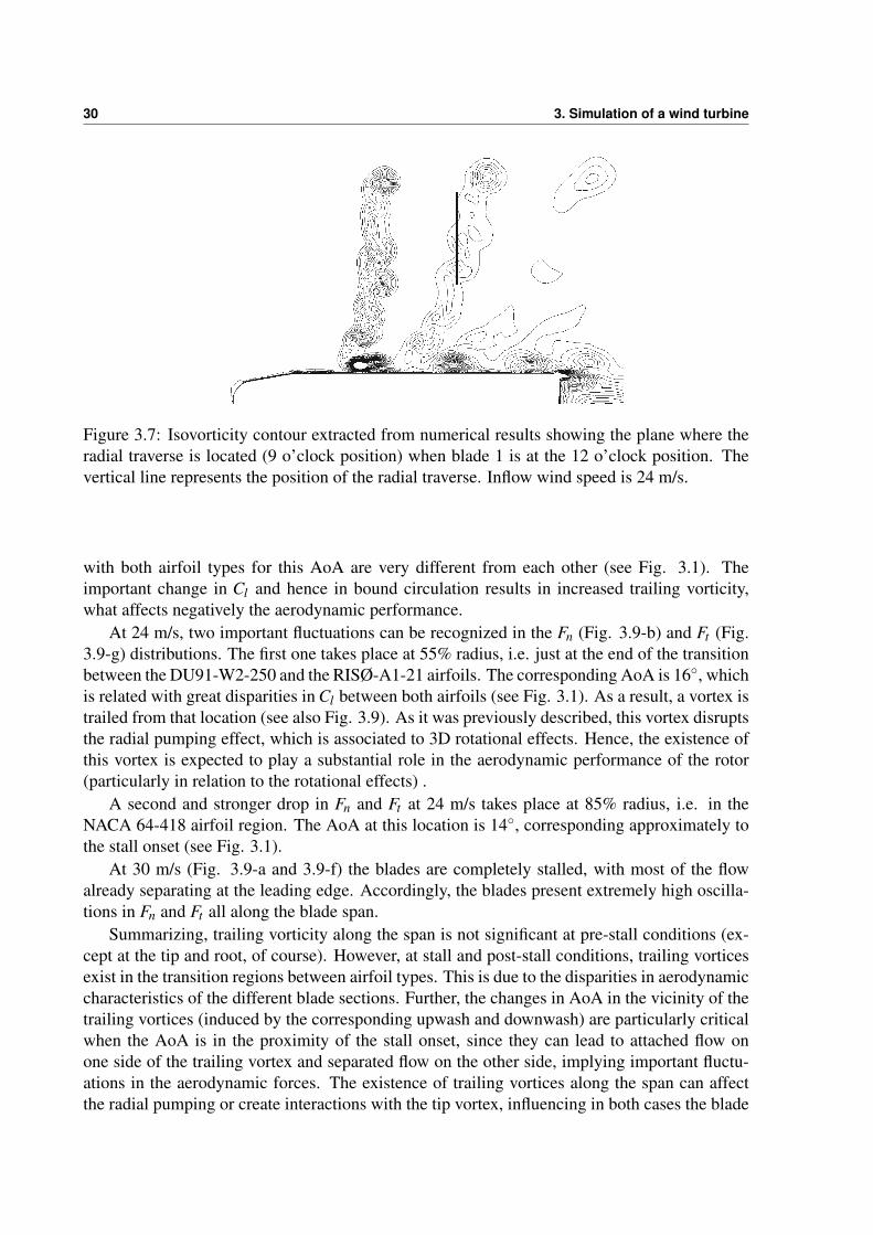
Figure 3.7: Isovorticity contour extracted from numerical results showing the plane where theradial traverse is located (9 o’clock position) when blade 1 is at the 12 o’clock position. Thevertical line represents the position of the radial traverse. Inflow wind speed is 24 m/s.
with both airfoil types for this AoA are very different from each other (see Fig. 3.1). Theimportant change in Cl and hence in bound circulation results in increased trailing vorticity,what affects negatively the aerodynamic performance.
At 24 m/s, two important fluctuations can be recognized in the Fn (Fig. 3.9-b) and Ft (Fig.3.9-g) distributions. The first one takes place at 55% radius, i.e. just at the end of the transitionbetween the DU91-W2-250 and the RISØ-A1-21 airfoils. The corresponding AoA is 16, whichis related with great disparities in Cl between both airfoils (see Fig. 3.1). As a result, a vortex istrailed from that location (see also Fig. 3.9). As it was previously described, this vortex disruptsthe radial pumping effect, which is associated to 3D rotational effects. Hence, the existence ofthis vortex is expected to play a substantial role in the aerodynamic performance of the rotor(particularly in relation to the rotational effects) .
A second and stronger drop in Fn and Ft at 24 m/s takes place at 85% radius, i.e. in theNACA 64-418 airfoil region. The AoA at this location is 14, corresponding approximately tothe stall onset (see Fig. 3.1).
At 30 m/s (Fig. 3.9-a and 3.9-f) the blades are completely stalled, with most of the flowalready separating at the leading edge. Accordingly, the blades present extremely high oscilla-tions in Fn and Ft all along the blade span.
Summarizing, trailing vorticity along the span is not significant at pre-stall conditions (ex-cept at the tip and root, of course). However, at stall and post-stall conditions, trailing vorticesexist in the transition regions between airfoil types. This is due to the disparities in aerodynamiccharacteristics of the different blade sections. Further, the changes in AoA in the vicinity of thetrailing vortices (induced by the corresponding upwash and downwash) are particularly criticalwhen the AoA is in the proximity of the stall onset, since they can lead to attached flow onone side of the trailing vortex and separated flow on the other side, implying important fluctu-ations in the aerodynamic forces. The existence of trailing vortices along the span can affectthe radial pumping or create interactions with the tip vortex, influencing in both cases the blade

3.3 Results and discussion 31
Figure 3.8: Streamlines of the relative wind speed over the blade upper surface, showing astrong standing vortex on the upper surface of every blade, which pumps air from the rootregion outwards. The inflow wind speed is 24 m/s.
performance.It is worth mentioning that Tangler (2004), who studied the experimental data of the NREL
UAE Phase VI wind turbine, made similar observations about the trailing vorticity in that rotor.More specifically, the author also suggested the existence (under certain conditions) of a mid-span vortex, which supposedly emanated from a standing vortex on the upper surface of theblade. Furthermore, he saw the same influence of the vortex-induced upwash and downwash onthe AoA. This indicates, that the effects observed in the MEXICO turbine might be commonalso in other rotors, even if their blade design is not based on airfoils with significant disparitiesin their characteristics (the UAE Phase VI blade is based exclusively on the S809 airfoil).
One more interesting feature of the Fn and Ft force distributions along the blade span is howthey evolve from low to high wind speeds: At low wind speeds (attached flow), the region ofthe blade producing the highest aerodynamic forces is the tip. When the wind speed increases(stall conditions), the tangential force, i.e. the force contributing the most to the driving torque,is greater at inboard locations. This is very meaningful, because inboard locations are subjectedto greater separation owing to the thicker airfoil type and greater AoA (the twist angle doesnot completely compensate for the higher inflow angle). The existence of rotational effects atinboard positions make therefore the rotating blades behaviour to differ substantially from sta-tionary blades, where flow separation is connected to a reduction in aerodynamic performance.

32 3. Simulation of a wind turbine
0 25 50 75 1000
100
200
300
r/R
Fn [N
/m]
100
200
300
400
Fn [N
/m]
200
300
400
500
Fn [N
/m]
300
400
500
600
Fn [N
/m]
300
400
500
600
700
Fn [N
/m]
0 25 50 75 100−10
0
10
20
r/R
Ft [N
/m]
20
40
60
Ft [N
/m]
20
40
60
80
Ft [N
/m]
20
40
60
80
100
120
140
Ft [N
/m]
50
100
150
200
Ft [N
/m]
(e) u = 10 m/s
(d) u = 15 m/s
(c) u = 19 m/s
(b) u = 24 m/s
(a) u = 30 m/s
(j) u = 10 m/s
(i) u = 15 m/s
(h) u = 19 m/s
(g) u = 24 m/s
(f) u = 30 m/s
Figure 3.9: Normal and tangential force along the blade span for 5 different wind speeds. Cir-cles are measurements and solid lines are simulations.

3.4 Conclusions 33
3.4 ConclusionsA CFD model of the MEXICO wind turbine based on the open source code OpenFOAM hasbeen successfully validated against experimental data. This validation enabled the synergeticuse of numerical and experimental results for the study of the trailing vortices and their interac-tion with the radial pumping effect, which in turn is related to the rotational effects that make3D blade characteristics to deviate substantially from 2D airfoil data. The authors infer that theuse of rather incompatible airfoil types of the MEXICO rotor leads to increased trailing vorticityat mid-span positions. In that region, the radial pumping effect is disrupted as a consequence ofa trailing vortex. This is believed to play an important role for the 3D rotational effects on theblade.

34 3. Simulation of a wind turbine

Chapter 4
Insight into the blade root flow1
Abstract The root flow of wind turbine blades is subjected to complex physical mechanismsthat influence significantly the rotor aerodynamic performance. Spanwise flows, the Himmel-skamp effect and the formation of the root vortex are examples of interrelated aerodynamicphenomena observed in the blade root region. In this study we address those phenomena bymeans of Particle Image Velocimetry (PIV) measurements and Reynolds Averaged Navier-Stokes (RANS) simulations. The numerical results obtained in this study are in very goodagreement with the experiments and unveil the details of the intricate root flow. The Himmel-skamp effect is shown to delay the stall onset and enhance the lift force coefficient Cl even at amoderate angle of attack (AoA ≈ 13). The results also show that the vortex emanating fromthe spanwise position of maximum chord length rotates in the opposite direction of the rootvortex, what affects the wake evolution.
4.1 IntroductionThe aerodynamic design of wind turbine blades is subjected to important levels of uncertainty.As a matter of fact, not only transient operational states can pose a challenge to the wind tur-bine designer, but also seemingly simple cases involving steady operation under axisymmetric,uniform inflow conditions (Leishman, 2002; Schepers, 2012). This is especially true for the tipand root regions of the blades, where the flow is three-dimensional and strongly influenced bythe trailing vortices (Micallef, 2012).
Spanwise flows and Himmelskamp effect
At the root of the blade, the angle of attack (AoA) is usually considerably higher than at thetip. This increases the complexity of the flow, since it often leads to flow separation, what inthis part of the blade generally gives rise to the Himmelskamp effect (Himmelskamp, 1947).This effect delays the stall onset and enhances the lift force as compared to non-rotating bladesoperating at the same AoA. The Himmelskamp effect, also known as stall delay or rotational
1Accepted for publication as discussion paper as I. HERRAEZ, B. AKAY, G.J.W. VAN BUSSEL, J. PEINKE andB. STOEVESANDT: Detailed Analysis of the Blade Root Flow of a Horizontal Axis Wind Turbine, Wind Energ.Sci..

36 4. The blade root flow
augmentation, has been studied by many authors both experimentally (Schreck and Robinson,2002; Sicot et al., 2008; Ronsten, 1992) and numerically (Guntur and Sørensen, 2014; Herraezet al., 2014; Schreck et al., 2007), although it still remains far from being well understood andcharacterized. It mainly affects the blade root region and is known to be closely related to theexistence of spanwise flows in the boundary layer. Snel et al. (1993) were the first to proposea correction model to be applied to 2D airfoil characteristics in order to account for this effectin Blade Element Momentum (BEM) and other engineering tools that rely in 2D airfoil data.More correction models have been developed since then (Chaviaropoulos and Hansen, 2000;Bak et al., 2006; Raj, 2000; Corrigan and Schillings, 1994, etc.). However, Breton et al. (2008)and Guntur et al. (2011) proved that their accuracy is still a critical issue. Currently, a majorimpediment in the development of accurate correction models is the incomplete understandingof the physical mechanisms. It is worth highlighting that, up to now, the study of the Him-melskamp effect has been mostly focused on post-stall conditions. Consequently, very little isknown about its onset at moderate angles of attack.
The root vortex
One fundamental feature of the root (and tip) flow is the formation of trailing vorticity that rollsup into a discrete vortex. Several authors have attempted to capture experimentally the rootvortex in the near wake of a wind turbine. However, as Vermeer et al. (2003) highlighted, thiscan be extremely difficult to achieve due to the fact that the near wake usually does not present adistinctive, well defined root vortex (opposite to the tip vortex). Many wind tunnel experimentswith model wind turbines confirmed this. For instance, Massouh and Dobrev (2007) and Haanset al. (2008) also came to that conclusion after studying a wind turbine rotor wake with ParticleImage Velocimetry (PIV) and hot film wake measurements, respectively. Furthermore, Ebertand Wood (2001) and Sherry et al. (2013) observed by means of PIV (among other measure-ment techniques) that the root vortex diffuses very rapidly. The PIV measurements performedby Akay et al. (2012b) on two different rotors demonstrated that the evolution and strength ofthe root vortex highly depends on the blade root geometry and the spanwise distribution of cir-culation. In a subsequent work also based on PIV measurements, Akay et al. (2014) suggestedthat the flow in the root region is driven by the bound vorticity.The study of the root (and tip) vortices can also be addressed by means of numerical simula-tions. For this purpose, Large Eddy Simulations (LES) are commonly combined with actuatorline models (Ivanell et al., 2007; Troldborg et al., 2007; Nilsson et al., 2015b). This technique isvery useful for analysing the evolution of the trailing vortices in the wake. However, it impliesa very strong simplification of the blade geometry, what makes it unsuitable for studying theorigin of the root and tip vortices. This is well exemplified in van Kuik et al. (2014), where itis concluded that the fact that actuator line models disregard the chordwise bound circulation atthe blade tip prevents them from computing correctly the tip vortex trajectory in the vicinity ofthe blade. The same article also shows that full blade Reynolds Averaged Navier-Stokes Simu-lations (RANS) as well as panel code computations allow a much more realistic study of the tipvortex formation mechanism. Indeed, the use of a panel code allowed Micallef et al. (2012) tostudy the origin of the tip vortex on a wind tunnel model rotor, unveiling the complex distribu-tion of bound vorticity at the blade tip. However, to the best of our knowledge, the origin of theroot vortex has still not been addressed in detail up to now.

4.1 Introduction 37
Scope and outlineThis article aims at gaining insight both experimentally and numerically into the root flow of ahorizontal axis wind turbine operating at design conditions. The focus is put into two importantand interrelated aspects of the root flow that, as above explained, are insufficiently understoodso far:
1. Spanwise flows and onset of the Himmelskamp effect at moderate angles of attack (designoperating conditions)
2. The origin of the root vortex
Section 4.2.1 and Sect. 4.2.2 describe the experimental and numerical set-up, respectively. Themain characteristics of the flow over the root region are presented in Sect. 4.3.1. Furthermore, inthis section the simulations are validated against experimental results. The presence of spanwiseflows is further discussed in Sect. 4.3.2. Section 4.3.3 addresses the onset of the Himmelskampeffect. The origin of the root vortex is analysed in Sect. 4.3.4. Finally, the main conclusions ofthis work are summarized in Sect. 4.4.

38 4. The blade root flow
0 0.2 0.4 0.6 0.8 10.05
0.1
0.15
0.2
0.25
Ch
ord
/ R
[−
]
r / R [−]
0 0.2 0.4 0.6 0.8 10
5
10
15
20
Tw
ist
[de
g]
Chord
Twist
Figure 4.1: Chord and twist distribution along the blade span.
4.2 Methods
4.2.1 Experimental setupThe scope of the experimental campaign is to measure the three components of the flow over theroot region of a wind turbine blade. This is achieved by means of stereoscopic Particle ImageVelocimetry (PIV).
The measurements are carried out in the Open Jet Facility of the Faculty of AerospaceEngineering at the Delft University of Technology. This wind tunnel has an octagonal open jetwith an equivalent diameter of 3 m. The studied wind turbine consists of a two-bladed rotorwith a diameter of 2 m. The chord and twist distributions are shown in Fig. 4.2.1. Table 4.1shows the used airfoil types.
Table 4.1: Airfoil type distribution along the blade spanRadial position range [r/R] Airfoil type
0.14 - 0.16 Cylinder0.16 - 0.21 Transition0.21 - 1.0 DU96-W-180
The measurement campaign includes both a spanwise and a chordwise configuration ofthe PIV windows. The spanwise measurements are carried out at different azimuth angles forcapturing the evolution of the near wake. In the chordwise configuration the PIV windows areorthogonal to the blade axis around the blade chord. This configuration, which included 40different radial positions, offers the best insight into the flow around the blade surface.
The measurements are phase-locked and phase-averaged with the azimuthal position of therotor blade rotation. This allows to reconstruct the flow over each blade section after measuringthe pressure and suction sides separately.

4.2 Methods 39
The rotor operated at rated conditions with a freestream wind speed U∞ = 6 m/s and arotational speed ω = 400 rpm (tip speed ratio λ = 7). The turbulence intensity is T I = 0.28%and there is no yaw misalignment. The Reynolds number at the radial position of maximumchord reached Re≈ 1.5×10⁵.
Further details about the experimental set-up can be found in Akay et al. (2014).
4.2.2 Numerical method and computational meshThe simulations presented in this work are based on the Reynolds-Averaged Navier-Stokes(RANS) method and they are performed with the open source code OpenFOAM (OpenFOAM,2015). The computational model solves the incompressible Navier-Stokes equations using afinite volume approach for the spatial discretization. The convective terms are discretized witha second order linear-upwind scheme. For the viscous terms a second-order central differenceslinear scheme is employed. The use of a non-inertial reference frame and the addition of theCoriolis and centrifugal forces to the momentum equations allows to account for the rotation ofthe system. The SIMPLE algorithm is employed for enforcing the pressure-velocity coupling.The turbulence in the boundary layer is modelled by means of the k−ω Shear-Stress Transport(SST) model proposed by Menter (1993).
The grid is generated with the software Pointwise (Pointwise, 2015). It exploits the sym-metry of the rotor by modelling only one half of it and using periodic boundary conditions.The computational domain is represented in Fig. 4.3 and it consists of two independent block-structured grids connected by means of a so called arbitrary mesh interface. The outer grid is a
Figure 4.2: Schematic representation of the computational domain. The inner cylinder repre-sents the arbitrary mesh interface.
semi-sphere with the radius 22R, where R is the blade radius. The inner grid, which containsthe blade, is a cylinder with the radius 1.1R and the height 1.1R. The motivation for using twostructured grids connected by an interface is to independently control the mesh resolution in theproximity of the blade and in the far field. The total number of cells is 9.8× 10⁶. The blade
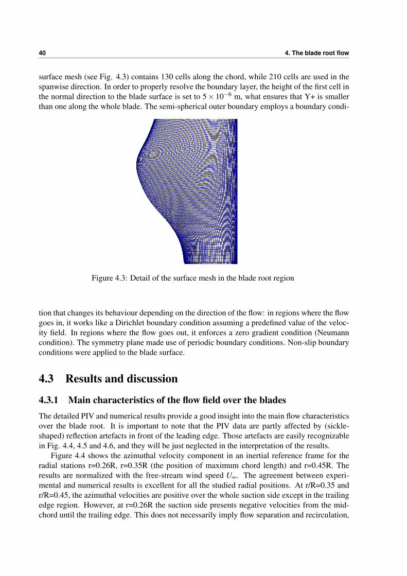
40 4. The blade root flow
surface mesh (see Fig. 4.3) contains 130 cells along the chord, while 210 cells are used in thespanwise direction. In order to properly resolve the boundary layer, the height of the first cell inthe normal direction to the blade surface is set to 5×10⁻⁶ m, what ensures that Y+ is smallerthan one along the whole blade. The semi-spherical outer boundary employs a boundary condi-
Figure 4.3: Detail of the surface mesh in the blade root region
tion that changes its behaviour depending on the direction of the flow: in regions where the flowgoes in, it works like a Dirichlet boundary condition assuming a predefined value of the veloc-ity field. In regions where the flow goes out, it enforces a zero gradient condition (Neumanncondition). The symmetry plane made use of periodic boundary conditions. Non-slip boundaryconditions were applied to the blade surface.
4.3 Results and discussion
4.3.1 Main characteristics of the flow field over the bladesThe detailed PIV and numerical results provide a good insight into the main flow characteristicsover the blade root. It is important to note that the PIV data are partly affected by (sickle-shaped) reflection artefacts in front of the leading edge. Those artefacts are easily recognizablein Fig. 4.4, 4.5 and 4.6, and they will be just neglected in the interpretation of the results.
Figure 4.4 shows the azimuthal velocity component in an inertial reference frame for theradial stations r=0.26R, r=0.35R (the position of maximum chord length) and r=0.45R. Theresults are normalized with the free-stream wind speed U∞. The agreement between experi-mental and numerical results is excellent for all the studied radial positions. At r/R=0.35 andr/R=0.45, the azimuthal velocities are positive over the whole suction side except in the trailingedge region. However, at r=0.26R the suction side presents negative velocities from the mid-chord until the trailing edge. This does not necessarily imply flow separation and recirculation,

4.3 Results and discussion 41
Figure 4.4: Experimental and numerical results of the azimuthal velocity component at differentblade spanwise positions.
though, since the relative velocity might still remain positive along the whole suction side. In-deed, at that radial position the local circumferential velocity caused by the blade rotation is1.82/U∞, what implies that the flow remains attached up to Uθ =−1.82/U∞. In Sect. 4.3.3 thelack of separation is demonstrated by means of the wall shear stress.
The axial flow component is shown in Fig. 4.5. The axial velocity over the second half of thesuction side becomes smaller with increasing radial position. This is in fact just a geometricaleffect that occurs as a consequence of the twist of the rotor blade. At r=0.45R the orientation ofthe second half of the suction side is slightly upstream, so the axial velocity becomes negativeif the flow is attached. The effect is smaller for lower radial positions because of the larger twist

42 4. The blade root flow
Figure 4.5: Experimental and numerical results of the axial velocity component at differentblade spanwise positions.
angle, which neutralizes the mentioned geometrical effect. The numerical results are consistentwith the experiments, although at r=0.45R the axial velocity over the suction side is slightlyoverpredicted.
Figure 4.6 displays the radial velocity component for the three considered spanwise posi-tions. At r=0.26R, this velocity is very strong on the suction side. However, at r=0.35R andr=0.45R it becomes much weaker. Hence, the presence of spanwise flows seems to be limitedto the innermost region of the blade. The agreement between experiments and simulations isagain very good for all three stations.
The velocity field 10 mm off the suction side has been extracted from both the numerical

4.3 Results and discussion 43
Figure 4.6: Experimental and numerical results of the radial velocity component at differentblade spanwise positions.
results and the available PIV data (including 40 different radial positions between r=0.17R andr=0.65R) in order to study the flow in the proximity of the blade surface in more detail. Fig. 4.7shows that the azimuthal component is always positive outboard of the position of maximumchord length (r=0.35R). Below that position, a significant region of the blade presents negativeazimuthal velocities close to the trailing edge. At r ≈ 0.3R, this effect is stronger in the PIVmeasurements than in the numerical results. Apart from this, the numerical results are in verygood agreement with the experimental results.
The axial flow velocity component is displayed in Fig. 4.8. Outboard of the radial positionof maximum chord length, the axial velocity becomes negative from the mid-chord towards the

44 4. The blade root flow
Figure 4.7: Experimental and numerical results of the azimuthal velocity component 10 mm offthe blade suction side
trailing edge. The same effect was already discussed in relation to Fig. 4.5. The fact that thenumerical results underpredict a bit this effect, which is caused by the relative position of thesuction side to the rotor plane, might indicate a possible small deviation in the pitch angle. Theagreement between PIV and CFD in the root region is very good, which is a clear indicationthat the wake and blade inductions are correctly predicted with the current CFD model.
Figure 4.6 presents the distribution of radial velocity along the blade suction side. Theexperimental results show a substantial spanwise flow in the leading edge region from r=0.45Routwards. This is rather surprising, since the flow in that region is fully attached (as shown forinstance in Fig. 4.7) and it is far away from the tip and root, where spanwise flows are usuallyexpected. The numerical results show much smaller radial velocities in that region. At presentthe authors do not have a solid explanation for this discrepancy. In the root region both PIV andCFD show evidence of strong spanwise flows in the proximity of the trailing edge, although thesimulation tends to underpredict the spanwise flow in the region 0.3R < r < 0.35R, as it alsohappened with the azimuthal velocity (Fig. 4.7). As stated earlier, this might be caused by aslight deviation of the pitch angle. Other than this, the consistency between PIV and CFD isagain very good, what gives confidence in the reliability of the numerical model in predictingthe complex flows of the root region.

4.3 Results and discussion 45
Figure 4.8: Experimental and numerical results of the axial velocity component 10 mm off theblade suction side
4.3.2 The source of the spanwise flowsTwo different explanations have been proposed in the literature for explaining the origin of thespanwise flows:
1. spanwise pressure gradients: the dynamic pressure over the blade surface is inverselyproportional to the radial position. Hence, the air is assumed to travel from the roottowards outer positions as a consequence of spanwise pressure gradients (Schreck andRobinson, 2002; Schreck et al., 2010).
2. centrifugal force: the centrifugal force that acts on the bottom of the boundary layer (i.e.the region where the flow is not detached from the surface) pushes the flow towards thetip (Lindenburg, 2003; Guntur and Sørensen, 2014).
In order to elucidate which is the actual source of the spanwise flows, the computed isobarsof the blade suction side are compared with the limiting streamlines (obtained from the wallshear stress) in Fig. 4.10. As it can be seen, the surface pressure does not present significantspanwise gradients. It is worth remarking that the same observation was made in the analysis

46 4. The blade root flow
Figure 4.9: Experimental and numerical results of radial velocity component 10 mm off theblade suction side
of the MEXICO wind tunnel experiment (Herraez et al., 2014). Therefore, we conclude that thecentrifugal force is the main source of spanwise flows.
Figure 4.10 also shows how the Coriolis force progressively redirects the spanwise flowcoming from the root towards the trailing edge, what makes the flow to follow a curved trajec-tory.
4.3.3 Onset of the Himmelskamp effectFigure 4.11 compares the pressure coefficient Cp distribution obtained from the blade atr=0.26R with the Cp distribution extracted from a 2D simulation at the same Reynolds num-ber (Re≈ 1×10⁵) and same angle of attack (AoA≈ 13, computed using the method proposedby Shen et al., 2009). The 2D simulation is a RANS computation performed with the k−ω SSTturbulence model. Also, the 2D mesh is equivalent to the 3D mesh except for the third dimen-sion. Experimental results of the same 2D airfoil with Re = 1×10⁶ are displayed as well. The2D experimental and numerical results present some disparity in the region of the suction peak,but apart from this they are very similar in spite of the difference of Reynolds number. However,the 3D results exhibit some important differences. The slope of the adverse pressure gradient is

4.3 Results and discussion 47
x / R [−]
r / R
[−]
0 0.05 0.1 0.15 0.2 0.25
0.4
0.35
0.3
0.25
0.2
0.15
Figure 4.10: Isobars and limiting streamlines over the suction side of the blade root region.
0 0.2 0.4 0.6 0.8 1
−3.5
−3
−2.5
−2
−1.5
−1
−0.5
0
0.5
1
x / c [−]
Cp [
−]
2D experiment
2D simulation
3D simulation
Figure 4.11: Cp distributions at AoA≈ 13. The corresponding Reynolds numbers are Re≈ 1×10⁶ for the 2D experimental results, Re≈ 1×10⁵ for the simulated 2D airfoil and Re≈ 1×10⁵
for the 3D blade (r=0.26R).

48 4. The blade root flow
substantially reduced, what leads to a delay of the separation point. The separation point can beapproximately identified as the point where the adverse pressure gradient meets the region withzero pressure gradient (i.e. the region where the flow is separated). In the 2D airfoils the sepa-ration point is located at x/c≈ 0.4. In the 3D case, the adverse pressure gradient presents a kinkat x/c ≈ 0.5, but it stays negative for the whole chord length, what seems to indicate that theflow remains attached. However, Sicot et al. (2008) concluded that rotating blades can presentseparation even in regions of adverse pressure gradient. In order to verify if there is separationin the 3D case, the skin friction coefficient C f x on the suction side is displayed in Fig. 4.12 forboth the 2D and 3D simulations. In the 2D case, C f x becomes positive at x/c = 0.39, indicatingthat the flow separates exactly at that point (in good agreement with the estimation from theCp distribution). In the 3D case, C f x becomes zero at x/c = 0.52, but it recovers directly af-terwards, remaining always negative. This confirms that the flow stays completely attached allalong the chord. The point where C f x becomes zero is actually the place where the chordwiseflow direction is deflected into a spanwise flow direction. The same happens for all other radialpositions at the root. Therefore, the transition between the chordwise and spanwise flows inFig. 4.10 can be considered as an isoline of C f x = 0.
Another remarkable feature of the 3D Cp distribution from Fig. 4.11 is that both the pressureand suction sides present approximately the same slope shortly after the kink in the adversepressure gradient (x/c ≈ 0.5) until the trailing edge. This resembles the behaviour of the 2Dcase in the region with zero pressure gradient. Finally, it is worth highlighting that the 3D casepresents a smaller suction peak than the 2D case.
The resulting lift and drag coefficients (Cl and Cd , respectively) for the 2D and 3D cases arepresented in Table 4.2. Cl is increased by approximately 9% as a consequence of the Himmels-kamp effect, whereas Cd does not seem to be influenced at all. This is also in agreement withour observations from the MEXICO turbine, where the Himmelskamp effect had a very limitedinfluence on the drag (Herraez et al., 2014).
Table 4.2: Cl and Cd for the simulated 2D airfoil and 3D blade at r=0.26R, AoA≈ 13
Cl Cd2D 0.97 0.073D 1.06 0.07
4.3.4 The origin of the root vortexThe bound vorticity γ can be computed as the difference in the velocity outside the boundarylayer of the pressure and suction sides. γ can then be decomposed into a radial γradial and achordwise γchordwise component. Figure 4.13 shows both components side by side.
γradial is concentrated around the 1/4 chord position, as might be expected. The radialcirculation Γradial can be computed from γradial as its integral along the chord: where ρ is theair density and Urel is the relative velocity in the plane perpendicular to the blade axis. Owingto the γradial distribution from Fig. 4.13 and the strong link between γradial and the lift, it can beconcluded that the lift force is generated almost exclusively in the first half of the chord all alongthe blade. The decay of γradial , and hence the decay of the lift force, is much more sudden at the

4.3 Results and discussion 49
0 0.2 0.4 0.6 0.8 1−15
−10
−5
0
5x 10
−3
x / c [−]
Cf
x [
−]
2D simulation
3D simulation
Figure 4.12: Wall shear stress in the chordwise direction over the suction side for the 2D and3D (r/R = 0.26) cases.
tip than at the root. As a consequence, the root losses take place much more gradually than thetip losses. This should be taken into account by the correction models used e.g. in the BEM andactuator line methods. γradial is transformed into γchordwise at the tip and root before becomingtrailed free vorticity, what gives rise to the tip and root vortices. This is evidenced in Fig. 4.13-b,where it can be seen that the tip and root regions present substantial γchordwise in the proximityof the trailing edge. γchordwise is distributed over a larger spanwise range at the root than at thetip, what is in agreement with the gradual root losses earlier described. Van Kuik et al. (2014)obtained very similar results at the tip of a different rotor but the root was not studied. In theinnermost region of the blade the sign of γchordwise at the trailing edge is opposite to that of thetip (as one would expect from a horseshoe vortex model). However, in the region of maximumchord length, γchordwise at the trailing edge presents the same sign as the tip vortex. The negativeγchordwise at the root implies an outward motion of the flow over the part of the suction side wherethe azimuthal velocity is slow (see Fig. 4.7). On the contrary, the positive γchordwise in the regionof maximum chord leads to an inward flow motion. Akay et al. (2014) studied the wake of thesame wind turbine with PIV and indeed observed the presence of an outward flow for r < 0.25Rand the existence of an inward flow in the radial range 0.25R < r < 0.35R. Furthermore, Mediciand Alfredsson (2006) did similar observations in their experimental wake study of a differentwind turbine. The present results not only confirm the mentioned experimental observations,but also explain the origin of this aerodynamic behaviour.
Figure 4.14 shows the bound vorticity vectors over the blade. From this figure it is evidenthow the direction of the bound vorticity γ changes at the root. As it can be seen, at the mostinboard part of the blade (r < 0.35R), γchordwise dominates the flow over the second half of thechord, indicating that vorticity is trailed along that region.
The fact that γchordwise is distributed over such a large area of the root might explain that

50 4. The blade root flow
Figure 4.13: Radial and chordwise components of the bound vorticity
the root vortex does not present a well defined, distinctive structure, as Vermeer et al. (2003),Massouh and Dobrev (2007) and Haans et al. (2008) reported in their experimental wake studiesof different wind turbines. Furthermore, the existence of two adjacent root regions with counter-rotating γchordwise might also explain the fast diffusion of the root vortex reported by Ebert andWood (2001) and Sherry et al. (2013).

4.3 Results and discussion 51
0 0.05 0.1 0.15 0.2
0.2
0.3
0.4
0.5
0.6
0.7
0.8
0.9
1
r/R
[−
]
x/R [−]
Figure 4.14: Bound vorticity vectors over the blade

52 4. The blade root flow
4.4 ConclusionsThe use of Particle Image Velocimetry (PIV) measurements and Reynolds-Averaged Navier-Stokes (RANS) simulations enabled the analysis of the flow in the root region of a wind turbineblade operating at design conditions with axisymmetric inflow. The following conclusions aredrawn:
• The RANS method is capable of capturing accurately the main features of the root flowof wind turbine blades operating at design conditions.
• The spanwise flows in the root region are caused by the centrifugal force and not by radialpressure gradients, as some authors have suggested.
• Even at relatively moderate angles of attack (AoA ≈ 13), the interaction of the centrifu-gal and Coriolis forces can give rise to the Himmelskamp effect.
• The influence of the Himmelskamp effect on the sectional Cp distribution is twofold: onone hand the suction peak is reduced, on the other hand the separation point is delayed(indeed in our case the separation is completely avoided). As a consequence of bothcounteracting effects, the influence of the Himmelskamp effect on the loads is weakerthan in the Cp distribution.
• The reduction of the aerodynamic performance is more gradual at the root than at the tip.Tip/root loss correction models (as used e.g. in BEM simulations) should account for thiseffect.
• The trailing vorticity in the spanwise position of maximum chord length presents theopposite sign than at the blade root. This contributes to the diffusion of the root vortex.
We recommend to consider these points for a better characterization of the root flow of windturbine blades. This can help to reduce the uncertainty of the blade design process, what in turnwould contribute to make the turbines more cost-effective.

Chapter 5
Insight into the role of 3D rotationaleffects1
Abstract Rotational effects are known to influence severely the aerodynamic performance ofthe inboard region of rotor blades. The underlying physical mechanisms are however far frombeing well understood. The present work addresses this problem using Reynolds AveragedNavier-Stokes computations and experimental results of the MEXICO rotor. Four axisymmetricinflow cases with wind speeds ranging from pre-stall to post-stall conditions are computed andcompared with pressure and PIV experimental data, obtaining in general consistent results. Atlow angles of attack, the aerodynamic behaviour of all the studied blade sections resembles theone from the corresponding 2D airfoils. However, at high angles of attack rotational effectslead to stall delay and/or lift enhancement at inboard positions. Such effects are shown tooccur only in the presence of significant radial flows. Interestingly, the way in which rotationaleffects influence the aerodynamics of the MEXICO blades differs qualitatively in certain aspectsfrom the descriptions found in the literature about this topic. The presented results providenew insights that are useful for the development of advanced and physically-sound correctionmodels.
5.1 IntroductionThe ever increasing size of wind turbine rotor blades requires accurate and efficient methodsfor the prediction of the aerodynamic loads and performance. Without a deep understandingof the flow phenomena governing the rotor aerodynamics, high levels of uncertainty must beexpected within the design process, implying a reduction in cost-effectiveness and reliability ofthe whole machine. Numerous difficulties have been identified in modelling the aerodynamicsof rotor blades (Leishman, 2002). Even stationary axial inflow conditions lead to complex flowphenomena, which are not yet well understood. Flow separation, secondary flows and stalldelay are examples of such interrelated phenomena, which furthermore are known to play a keyrole in the aerodynamic behaviour of the rotor. Those effects, being highly three-dimensional(3D), limit substantially the applicability of two-dimensional (2D) airfoil polars for their use in
1Published as I. HERRAEZ, B. STOEVENSADT and J. PEINKE: Insight into Rotational Effects on a WindTurbine Blade using Navier-Stokes Computations, Energies, 7, 6798–6822, 2014.

54 5. The role of 3D rotational effects
the design process. Therefore, 2D polars need to be corrected for rotational effects before usingthem in aeroelastic codes and other design tools.
Simms et al. (2001) reported the results of a blind test comparison in which different aerody-namic models were used for simulating the NREL Unsteady Aerodynamics Experiment (UAE)Phase VI turbine. The computed results, which were obtained with numerical tools rangingfrom Blade Element Momentum (BEM) theory to wake and Computational Fluid Dynamics(CFD) codes, showed a great level of uncertainty. The discrepancies observed between exper-iments and computations were attributed to the difficulty of predicting correctly the effect ofrotation on rotor blades. This highlights the importance of improving the correction models forrotational effects and at the same time it stresses the necessity of gaining a deeper understandingof the underlying physical mechanisms.
The study of rotational effects dates back to the mid-20th century. Himmelskamp (1947)studied experimentally rotational effects on aircraft propellers and observed lift enhancementand stall delay in rotating blades as compared to non-rotating blades. Banks and Gadd (1963)performed a theoretical analysis for steady boundary layers and inferred that rotation helps todelay stall, especially in the blade root region. McCroskey and Yaggy (1968) showed thatcrossflows contribute to the delay of separation on rotating helicopter blades. A rotating and anon-rotating wind turbine blade were compared experimentally by Ronsten (1992), concludingthat rotational effects were significant only in the proximity of the hub. Wood (1991) describedstall delay in terms of pressure changes to the external inviscid flow and observed that it dependson the local solidity of the blades. The use of 3D steady momentum integral boundary layerequations allowed Du and Selig (2000) to discern the importance of the Reynolds number forrotational effects on a wind turbine, deducing that for large wind turbines rotational effectswould be of less importance than for small turbines. Schreck and Robinson (2002) investigatedsurface pressure measurements from the NREL UAE Phase VI experiment and observed thatrotational augmentation is connected to radial surface pressure gradients. Tangler (2004) alsostudied the experimental data from the same wind turbine and highlighted the importance of thetrailing vorticity and rotational effects for the aerodynamic performance. An experimental workby Sicot et al. (2008) on a small wind turbine, compared sectional surface pressure distributionsfrom a rotating and a non-rotating blade operating in turbulent flow. The root region of the bladepresented enhanced lift, but no evidence of stall delay was observed.
CFD simulations have also been commonly used since the last 15 years for the analysisof rotor aerodynamics. Different types of simulation codes have been validated against mea-surements since then. Duque et al. (1999) and Duque et al. (2003) obtained reasonable results(specially at attached flow conditions) simulating the NREL Combined Experiment Phase IIand the NREL UAE Phase VI turbines with a RANS unsteady compressible code that madeuse of overset grids and the Baldwin-Lomax algebraic turbulence model. Le Pape and Lecanu(2004) used another unsteady compressible RANS code with the kω and the kω − SST turbu-lence models for simulating the NREL Phase VI turbine. The best results were obtained with thekω−SST model, but the predictions at stall conditions were rather inaccurate with both mod-els. Johansen et al. (2002) used Detached-Eddy Simulations based on the kω−SST turbulencemodel for predicting the flow around the NREL Phase VI turbine under parked conditions withfixed pitch as well as with oscillating pitch. The DES results presented more three-dimensionalflow structures than RANS simulations, but the global blade characteristics were not better pre-dicted. Johansen and Sørensen (2004) simulated 3 different wind turbines with RANS using the

5.1 Introduction 55
kω−SST model and one turbine using DES. The authors highlighted the challenges associatedto the prediction of highly separated rotor flows.Sørensen and Schreck (2012) obtained goodresults of the flow field upstream and downstream of the MEXICO turbine in axial and yawedconditions using the kω turbulence model.In general, most CFD codes obtained better results simulating the NREL UAE Phase VI turbinethan the MEXICO turbine. Sørensen et al. (2002) explained that the NREL turbine was compar-atively well suited for the computation with the RANS method because its blades are designedwith the S809 airfoil, for which good results at high angles of attack (AoA) are obtained alsowith 2D simulations. Furthermore that airfoil type is apparently rather insensitive to the vortexinteraction in the wake, what facilitates its prediction with RANS. The authors also studied ro-tational effects in that wind turbine, concluding that the enhancement of the aerodynamic forcesat inboard radial positions was attributed to radial pumping of the separated flow in the inboardblade region. In a later work, Schreck et al. (2007) studied the same turbine using RANS withthe kω − SST turbulence model and ascribed the rotational effects to stationary vortical struc-tures located on the upper blade surface. Very recently, Guntur and Sørensen (2014) studiedthe MEXICO turbine with RANS and the kω model, observing that on rotating blades there isa postponement of the separation point. Furthermore it was concluded that the AoA at whichseparation is initiated is higher in 3D compared with 2D.
The knowledge gained from measurements, theoretical works and numerical computationshas been used by several authors for developing correction models for 2D polars (Snel et al.,1993; Chaviaropoulos and Hansen, 2000; Raj, 2000; Bak et al., 2006; Lindenburg, 2003; Cor-rigan and Schillings, 1994; Tangler and Selig, 1997; Du and Selig, 1998). Breton et al. Bretonet al. (2008) compared six different correction models for rotational effects using a lifting-lineprescribed wake vortex code for simulating the NREL UAE phase VI turbine. None of the mod-els was able to predict the measured data satisfactorily and the loads under stall conditions weregenerally overestimated. Guntur et al. Guntur et al. (2011) performed a similar test with exper-imental data from the MEXICO wind turbine, using an inverse BEM method for determiningthe AoA. Again, none of the correction models was successful at predicting the 3D aerodynamiccharacteristics.
As shown, current knowledge about rotational effects is still incomplete and requires furtherinvestigation if rotor blades are to be designed in a more reliable and cost-effective way.
The present work addresses this problem using a CFD model of the MEXICO wind turbinein conjunction with experimental data. The existence of rotational effects is verified by compar-ing 2D and 3D airfoil polars. Then, 2D and 3D Cp distributions are analysed for ascertainingthe mechanisms that lead to an augmentation of the lift force at inboard positions. A deeperinsight into the sources of the rotational effects is gained through the study of distinctive flowfeatures in the near wake and the boundary layer of the rotor blades. The knowledge gainedfrom these analyses is compared throughout the paper with the findings from other studies andthe assumptions from well-known correction models. This provides important information forthe development of improved and physically-sound correction models.

56 5. The role of 3D rotational effects
5.2 Methods
5.2.1 The MEXICO ExperimentThe EU FP5 MEXICO (Model EXperiments In COntrolled COnditions) project involved theextensive measuring of loads, surface pressure and flow field data of a three bladed 4.5 mrotor diameter wind turbine placed in the Large Low-Speed Facility of the German-Dutch Windtunnel DNW, which has an open Section of 9.5 x 9.5 m2 (Schepers and Snel, 2007). Theblockage ratio was 18% but the use of breathing slots behind the collector helped to reducetunnel effects. Rethore et al. (2011) and Shen et al. (2012) showed that tunnel effects have verylimited influence on the rotor flow.
The design of the blades was based on 3 different aerodynamic profiles, as shown in Table5.1.
Table 5.1: Airfoil type distribution along the span of the MEXICO bladeRadial position [r/R] Airfoil type
0.09-0.17 Cylinder0.17-0.20 Transition0.20-0.50 DU91-W2-2500.50-0.54 Transition0.54-0.70 RISØ-A1-210.70-0.74 Transition0.74-1.00 NACA 64-418
The blades were twisted and tapered, and a zig-zag tape at 5% of the chord was used bothon the blade upper and lower surfaces to trigger the laminar to turbulent transition.
The tower was located 2.13 m downwind from the rotor and its diameter was only 0.5 m, soits influence on the rotor flow is believed to be negligible (Bechmann et al., 2011; Shen et al.,2012). The measurements were performed under different inflow conditions. In this work fourwind speeds have been considered, namely 10, 15, 19 and 24 m/s. The rotational speed and thepitch angle were kept constant at 424.4 rpm and -2.3, respectively. Only axial inflow conditionsare considered in order to isolate the rotational effects from other influences like dynamic stall.
The pressure measurements were performed by means of pressure transducers placed atfive different blade sections corresponding to the blade span positions 0.25R, 0.35R, 0.60R,0.82R and 0.92R. Multiple PIV windows upstream and downstream of the turbine were usedfor measuring the flow field. Furthermore, the loads on the tower bottom were measured bymeans of a balance.
The tip speed was 100 m/s for all cases, meaning a tip speed ratio of 6.7 at design con-ditions (U∞=15 m/s). The Mach number did not exceed 0.3, and compressibility effects areconsequently disregarded in this work.
Table 5.2 shows the chord-based Reynolds and Rossby numbers of the MEXICO turbineat different radial positions. For comparison with a large turbine, the same parameters corre-sponding to the NREL 5 MW wind turbine (Jonkman et al., 2009) are shown. In both cases,

5.2 Methods 57
rated operating conditions have been assumed. The Reynolds number in the MEXICO turbineis one order of magnitude smaller than in the NREL 5 MW turbine, indicating that the viscousforces play a substantially stronger role in the MEXICO turbine. However, the Rossby numberis similar for both machines (on average it is just about 17% smaller in the MEXICO turbine),what implies that the effect of rotation in both cases is probably comparable. Furthermore, theRossby number decreases towards the blade root, what in turn means that the influence of theCoriolis force in that blade region is stronger.
Table 5.2: Reynolds and Rossby numbers for the MEXICO (subscript MX) and the NREL 5MW (subscript NREL) wind turbines at different radial positions.
r/R ReMX RoMX ReNREL RoNREL
0.25 4.3×10⁵ 2.9 7.0×10⁶ 3.90.50 5.5×10⁵ 7.4 1.0×10⁷ 8.70.75 6.2×10⁵ 14.1 1.2×10⁷ 15.80.90 6.2×10⁵ 20.1 1.2×10⁷ 23.3
The MEXICO data set (Boorsma and Schepers, 2003) also includes wind tunnel measure-ments of the 2D airfoils shown in Table 5.1. The Reynolds numbers from the 2D experimentsare approximately in the range corresponding to the blades. Furthermore, the 2D airfoils werefitted with a zig-zag tape in the same fashion like the blades for triggering the transition fromlaminar to turbulent flow. The 2D experiments include both lift and drag characteristics aswell as Cp distributions (except for the RISØ-A1-21 airfoil, for which only aerodynamic forcecoefficients are available).
It would be very useful to count with blade section characteristics obtained from parkedrotor experiments in order to isolate rotational effects from possible 3D effects caused by theblade geometry. Such experiments were also carried out within the MEXICO project, but thecorresponding measurement results are unfortunately not reliable because of malfunctioningpressure sensors (Pascal, 2009). However, the main differences between 2D and 3D results areknown to occur in the post-stall range, especially in the inboard region, where rotational effectsclearly dominate over other influences (Sicot et al., 2008; Schreck et al., 2007). Therefore, weassume that comparing 2D and 3D characteristics is an acceptable method for assessing therole of the rotational effects. This is also the most common way to do it (Bechmann et al.,2011; Guntur and Sørensen, 2014; Johansen and Sørensen, 2004; Le Pape and Lecanu, 2004;Sørensen et al., 2002; Tangler, 2004; Troldborg et al., 2013; Breton et al., 2008; Guntur et al.,2011).
Further details about the experimental set-up can be found in Boorsma and Schepers (2003).
5.2.2 Numerical method and computational meshThe numerical results presented in this work have been obtained from incompressible steadystate Reynolds Averaged Navier-Stokes (RANS) simulations performed with the open sourcesoftware OpenFOAM. OpenFOAM is a computational framework for numerical simulations ofpartial differential equations. The rotation of the system was accomplished using a non-inertial

58 5. The role of 3D rotational effects
reference frame and adding the Coriolis and centrifugal forces to the momentum equations.The SIMPLE algorithm was employed for the pressure-velocity coupling. The convective termswere discretized with a second order linear-upwind scheme. The discretization of the viscousterms was achieved by means of a second order central-differences linear scheme. The spatialdiscretization was performed with the finite volume method. No time discretization was usedsince only steady-state simulations were performed. The simulations were run fully turbulentand made use of the Spalart and Allmaras (1994) turbulence model. The use of a so called adap-tive (also known as continuous) wall function allowed to maintain a comparatively low numberof cells without compromising the accuracy of the simulations under separated flow conditions.The way in which the adaptive wall function works is simple: it switches automatically betweena low-Re and a high-Re computation approach in dependence of the local Y+ value. In regionswhere the first grid point is within the viscous sublayer (small Y+), the low-Re approach isfollowed and the boundary layer is completely resolved. In areas where the first grid point is inthe log-law region (high Y+), a wall function is used. A blending function is also implementedfor the cases where the first grid point is within the buffer layer, i.e. between the viscous sub-layer and the log-law region. When the flow is separated or close to the separation point, theflow velocity becomes very low, what implies that Y+ will be also very small. The boundarylayer will be then fully resolved instead of modelled with a wall function. This is a substantialenhancement as compared to standard wall functions, since it allows a satisfactory prediction ofcomplex flow conditions including stall (Spalding, 1961; Rung et al., 2001; de Villiers, 2006;Mockett, 2009; Schmidt et al., 2009).
In OpenFoam the velocity-pressure coupling is based on a collocated grid approach (boththe velocity and the pressure are solved at the centre of the control volumes). This implies thatboth the velocity and the pressure conditions have to be defined at all boundaries. At the inlet,the wind speed was specified and the pressure was set to zero gradient. On the contrary, at theoutlet the pressure was predefined and the velocity was set to zero gradient. Non-slip boundaryconditions were set for the blades and the nacelle.
The parallelization of the simulations was accomplished by means of the Message PassingInterface (MPI).
The iterative convergence was ensured by achieving at least three orders of magnitude re-duction in the residuals of each field variable. Furthermore, in order to guarantee that the nu-merical results are grid independent, a grid convergence study was performed prior to carryingout the simulations presented in this paper. The study was based on the Grid Convergence In-dex (GCI) method developed by Roache (Roache, 1994, 1998a), which is used for quantifyingthe numerical uncertainty. For this, the MEXICO rotor was simulated at design conditions (i.e.15 m/s and axisymmetric flow) with three different meshes. After generating a coarse mesh(5.8×10⁶ cells), it was systematically refined for creating the medium (8.5×10⁶ cells) and fine(11.3×10⁶ cells) meshes.
Table 5.3 summarizes the results of the study for the key variables torque and thrust. φ
represents the corresponding key variable, whereas eext and GCI represent the extrapolatedrelative error and the numerical uncertainty, respectively, both referred to the fine grid. The lowuncertainty level obtained for both the torque and the thrust (0.42% and 0.55%, respectively)is a clear indicator, that the results with the fine mesh are grid independent. That mesh wastherefore used for all the simulations presented in this paper.
The mesh exploited the 120-degrees symmetry of the wind turbine rotor by modelling only

5.3 Results and discussion 59
Table 5.3: Results of the grid convergence studyφ=Torque φ=Thrust
φ f ine 101.97 Nm 569.97 Nφmedium 102.03 Nm 570.40 Nφcoarse 102.25 Nm 576.76 Neext 0.34% 0.44%GCI 0.42% 0.55%
one blade. The domain consisted of 1/3 of a cylinder and employed periodic boundary con-ditions in order to account for the other two blades. Its length and radius were 52 and 16 m,respectively. The mesh was of type unstructured and hex-dominant (99% of the cells werehexaedra, the rest were split hexaedra). The boundary layer of the blades and the nacelle wasresolved with 5 prism-layers. The use of the adaptive wall function allowed for a y+ value onthe blades between 50 and 200 under attached flow conditions, which helped to limit the num-ber of cells. The wake and the regions where high gradients were expected, were accordinglyrefined.
5.3 Results and discussion
5.3.1 3D aerodynamic characteristicsAs mentioned in Section 5.1, the aerodynamic characteristics extracted from rotating bladescommonly present evidence of rotational effects such as stall delay and lift enhancement (es-pecially at radial positions close to the blade root). In order to verify the existence of sucheffects in the MEXICO turbine, the measured and computed lift coefficient (Cl) characteristicsfrom different blade radial positions are compared with experimental 2D Cl characteristics inFig. 5.1. The same comparison for the drag coefficient (Cd) is shown in Fig. 5.2. Every plotin those figures shows four points for the 3D experimental results. Every point corresponds toa different wind speed (U∞ = 10, 15, 19 and 24 m/s). Owing to the constant pitch angle androtational speed, increasing wind speed implies increasing AoA. The full lines representing thenumerical results were also obtained from the above mentioned four free-stream wind speeds.
The 3D polars have been extracted from the numerical and experimental results followingthe method described in Johansen and Sørensen (2004). For this, the normal force coefficient(Cn) and tangential force coefficient (Ct) have been computed from the surface pressure co-efficient (Cp) distributions and then transformed into Cl and Cd after calculating the AoA. Thecalculation of the AoA is based on the method proposed by Hansen et al. (1997), which relies onflow field data extracted from numerical simulations, and has proven to be reliable (Johansenand Sørensen, 2004; Sørensen et al., 2002; Guntur and Sørensen, 2012). In this method, thewind speed is sampled along multiple rings both upstream and downstream of the rotor. Theradius of the rings corresponds to the spanwise positions for which the AoA should be obtained.Then, the average velocity for each ring is calculated. Afterwards, the velocity in the rotor planefor each radius is computed by interpolating along the axial direction the mean velocities ob-

60 5. The role of 3D rotational effects
0 10 20 300
0.5
1
1.5
2
2.5
3
AoA [deg]
Cl [
−]
0 10 200
0.5
1
1.5
2
2.5
AoA [deg]
Cl [
−]
0 10 200
0.5
1
1.5
2
AoA [deg]
Cl [
−]
0 5 10 150
0.5
1
1.5
2
AoA [deg]
Cl [
−]
0 5 10 150
0.5
1
1.5
2
AoA [deg]
Cl [
−]
a) b) c)
d) e)
r=0.25R r=0.35R r=0.60R
r=0.82R r=0.92R
Figure 5.1: Comparison of Cl characteristics at five different spanwise positions. The dottedlines represent 2D experimental results, the circles indicate 3D experimental results and the fulllines show 3D numerical results.

5.3 Results and discussion 61
0 10 20 300
0.1
0.2
0.3
0.4
0.5
0.6
AoA [deg]
Cd [−
]
0 10 20 300
0.1
0.2
0.3
0.4
AoA [deg]
Cd [−
]
0 10 200
0.05
0.1
0.15
0.2
AoA [deg]C
d [−
]
0 5 10 150
0.05
0.1
0.15
0.2
AoA [deg]
Cd [−
]
0 5 10 150
0.05
0.1
0.15
0.2
AoA [deg]
Cd [−
]a) b) c)
d) e)
r=0.25R r=0.35R r=0.60R
r=0.82R r=0.92R
Figure 5.2: Comparison of Cd characteristics at 5 different spanwise positions. The dotted linesrepresent 2D experimental results, the circles indicate 3D experimental results and the full linesshow 3D numerical results.

62 5. The role of 3D rotational effects
tained in the previous step. Finally, the effective angle of attack is estimated with the followingequation:
AoA = arctan(
Urotor
rω
)−φ , (5.1)
where, Urotor is the axial wind speed in the rotor plane, ω is the rotational speed, r is the localradius and φ is the local angle between the chord of the blade section and the rotor plane,considering both the pitch and the twist angles.
3D Cl characteristics
In the proximity of the blade root, i.e. at r = 0.25R (Fig. 5.1-a), the experimental 3D Cl char-acteristics are almost identical to the 2D case until the 2D airfoil begins to stall (approximatelyat AoA = 12). After having reached that angle, only the 3D Cl curve continues to rise. Indeed,that Cl curve does not present any evidence of stall for the whole range of available data, whichgoes until AoA = 26. Taking into account that the AoA of stall onset for the 2D case is ap-proximately 12, the lack of stall in the 3D case implies a delay in the stall AoA of at least 14,i.e. the stall onset is delayed by 117%. At AoA = 26, the 3D Cl curve presents 115% more liftthan the 2D case for the same AoA and 55% more lift than the maximum lift from the 2D case.The simulations agree quite well with the measurements and are able to predict satisfactorilythe stall delay and lift enhancement.
A bit further outboard, at r = 0.35R (Fig. 5.1-b), the experimental 3D Cl characteristicsagain resemble the 2D curve up to the 2D stall onset, although the slope of the 3D curve isslightly greater when the stall AoA is approached. At higher AoA, the 3D case presents liftenhancement as compared with the 2D curve. However, the slope of the 3D Cl characteristicsbecomes less steep after the 2D stall onset, meaning that rotational effects are less strong atthis position than at r = 0.25R. In fact, the stall angle does not seem to be delayed, in spite ofthe maximum lift being enhanced by approximately 15%. At this radial station the numericalresults are consistent with the 3D experimental results up to the 2D stall onset. For higher AoA,the simulations overpredict a bit the Cl values, although they offer a good qualitative agreementwith the experiments.
In the proximity of the mid-span region, i.e. r = 0.60R (Fig. 5.1-c), the experimental 2Dand 3D Cl characteristics are similar until the stall onset. From the experimental results, itseems that at AoA = 12, i.e. shortly after the 2D stall onset, the rotating blade produces less liftthan the 2D airfoil. However, at AoA = 17 (i.e. in the post-stall region), the blade maintainsalmost the same Cl as the maximum Cl from the 2D airfoil, indicating the existence of stalldelay. Measurements and simulations present a good qualitative and quantitative agreement forthe whole range of available AoA except for AoA = 12, where the simulations overpredict thelift.
At r = 0.82R (Fig. 5.1-d) and more markedly at r = 0.92R (Fig. 5.1-e), the experimental3D results display a lower Cl than the 2D airfoil for the whole range of AoA, although thiseffect is significantly stronger after the stall onset. At low AoA, the Cl reduction is attributedto the influence of the tip vortex on the local induction. At high AoA, it seems to exist anadditional source of Cl reduction, which is discussed later in more detail. The simulationspredict satisfactorily the linear range but overestimate Cl at high AoA. Here, it is worth to recallthat other CFD investigations from the MEXICO turbine encountered the same difficulties in

5.3 Results and discussion 63
the outboard region. As an example, the final report of the MexNext project (Schepers et al.,2012) shows a comparison of the Cp distributions obtained from different CFD models. At U∞
= 24 m/s, the results for r = 0.82R and r = 0.92R from six different models out of seven presenta good consistency between them. However, all the mentioned models overpredict the negativepressure on the attached flow region of the suction side, what implies an overestimation of Cl .
Breton et al. (2008), who used a lifting line prescribed wake vortex code for simulating theNREL UAE Phase VI turbine, documented that most correction models for rotational effectslead to an overprediction of the lift in the outermost region of the blade. Only two exceptionswere identified: the model by Corrigan and Schillings (1994), who suggested not to apply anycorrection for rotational effects above r = 0.75R, and the model by Lindenburg (2003), whosuggested not only not to apply any lift-enhancement correction above r = 0.80R, but also tointroduce a special tip loss correction for accounting for radial flows above that radial position.The results from the MEXICO turbine confirm that it is a good idea to limit the enhancementof the lift force at outboard positions. The suitability of the special tip loss correction proposedby Lindenburg is discussed later in connection with the drag.
3D Cd characteristics
In opposition to the 3D Cl characteristics, the 3D Cd characteristics (Fig. 5.2) are more or less ingood agreement with the 2D characteristics at r = 0.25R and r = 0.35R for the whole range ofavailable AoA (even under stall conditions). The simulations are in general consistent with theexperiments, except at the highest AoA, where Cd is underestimated. Furthermore, at r = 0.35Rthe simulations tend to slightly underestimate Cd for the whole range of AoA.
At r = 0.60R (Fig. 5.2-c) the experimental 3D Cd characteristics resemble again the 2Dcase, except at AoA = 17, where the 3D drag is reduced as compared with the 2D case. As itwas seen in the Cl characteristics for the same radial position and AoA, rotational effects playa significant role at these conditions. The Cd reduction is therefore attributed to the mentionedeffects. The numerical results are also reasonably consistent with the experiments at this station.At AoA = 17 the simulations overestimate Cd , though.
The way in which rotational effects influence the Cd characteristics of the MEXICO rotorblades differs from the descriptions found in the literature about this topic: as an example, in theNREL UAE Phase VI wind turbine, rotational effects were accompanied by a significant dragincrease (Sørensen et al., 2002; Breton et al., 2008; Johansen and Sørensen, 2004). Additionally,Lindenburg (2003) describes rotational effects to increase the drag as a consequence of theradial flows existing in rotating blades under stall conditions, arguing that energy is required forpumping air from the root region towards outer radial positions. Furthermore, most correctionmodels for rotational effects predict a Cd increase (Bak et al., 2006; Raj, 2000; Lindenburg,2003), while others describe a Cd reduction (Du and Selig, 2000; Corrigan and Schillings, 1994)or no influence at all on Cd (Snel et al., 1993). Owing to the fact that in the MEXICO turbinerotational effects do not affect substantially Cd , except at r = 0.60R, it is not surprising that inthe study by Guntur et al. (2011), who tested different correction models with the MEXICOturbine, it is concluded that correcting for Cd might be unnecessary (their study was limited tothe radial stations r = 0.25R and r = 0.35R). That conclusion, which our results confirm for thesame turbine, can however not been generalized for other wind turbines (as explained above).Furthermore, the fact that in the MEXICO turbine rotational effects influence Cd at r = 0.60R,

64 5. The role of 3D rotational effects
but do not do it at r = 0.25R and r = 0.35R, is an indication that such effects might be airfoiltype-dependent (at r = 0.25R and r = 0.35R, the DU91-W2-250 airfoil was used, whereas atr = 0.60R the RISØ-A1-21 airfoil was utilized).
At r = 0.82R as well as at r = 0.92R (Fig. 5.2-d and Fig. 5.2-e, respectively), the exper-imental Cd from the 3D case is increased as compared with the 2D airfoil, especially at highAoA. The influence of the tip vortex and the subsequent downwash at radial positions r < Rimply a reduction of the AoA, what also leads to a reduction of Cl and Cd . The Cd rise observedin the MEXICO turbine indicates that other influences must be taken into account. Lindenburg(2003) suggested that the influence of the radial flows coming from inboard positions should beconsidered for modelling the airfoil characteristics at outboard positions. Therefore, his modelfor rotational effects includes a special correction for r > 0.8R, which is based on the idea thatthe spanwise flows acting on the separated volume of air can not be driven further outboardthan the blade tip itself, what causes a pressure rise on the suction side of the tip region. Asa consequence, he expected Cl and Cd to drop. This is in conflict with the Cd rise observed athigh AoA in Fig. 5.2-d and Fig. 5.2-e, so Lindenburg’s suggestion does not seem adequate forthe MEXICO wind turbine.
The CFD results for r = 0.82R and r = 0.92R present the problem that the drag is under-predicted at high AoA. Even for 2D airfoils, the prediction of the aerodynamic loads under stallconditions is known to be a challenge for RANS computations (Bertagnolio et al., 2001), so themismatch with the experiments are probably due to the limitations of the RANS method. Theselimitations for the prediction of separated flows mainly arise from two issues: First, turbulenceis not resolved, but modelled. The turbulence models are usually designed and calibrated forcertain applications and conditions, and they are by no means universally reliable. Complexflow situations like flow separation are certainly a major challenge for any turbulence model.Secondly, RANS is not able to resolve the unsteadiness associated to separated flows becauseit only provides an averaged solution, what of course can lead to poor predictions in the stallregion. However, this problem is expected to be of less importance in the blade root region,where separation is known to be a rather stationary process because of the stabilizing standingvortex that characterizes stall in that part of the blade (Schreck and Robinson, 2002; Robinsonet al., 1999).
However, it remains unclear why under stall conditions the experimental results for r =0.82R and r = 0.92R show that the lift reduction is accompanied by a drag increase as comparedwith the 2D airfoil. This problem is further discussed in the Sections 5.3.3 and 5.3.4.
5.3.2 Influence of rotational effects on the Cp distributionsThe 3D airfoil characteristics have shown that, under stall conditions, stall delay and/or lift en-hancement influence the aerodynamic performance of the blade at the radial positions r = 0.25R,r = 0.35R and r = 0.60R. In order to study in more detail the origin of those effects, the com-puted and measured Cp distributions of the mentioned radial positions are presented in Fig.5.3-5.5 for U∞ = 24 m/s (corresponding to the wind speed at which the strongest rotationaleffects occur). In Fig. 5.3 and Fig. 5.4 (r = 0.25R and r = 0.35R, respectively), the exper-imental Cp distributions from the corresponding 2D airfoil (DU91-W2-250) are also shown.Unfortunately, for the station r = 0.60R, which uses the airfoil RISØ-A1-21, no experimentalCp distribution of the 2D airfoil is available.

5.3 Results and discussion 65
0 0.2 0.4 0.6 0.8 1
−10
−8
−6
−4
−2
0
x/c [−]
Cp [−
]
Figure 5.3: Cp distribution from r = 0.25R for U∞ = 24m/s, corresponding to AoA = 26. Thedotted line represents 2D experimental results, the circles indicate 3D experimental results andthe full line shows 3D numerical results.
0 0.2 0.4 0.6 0.8 1
−8
−7
−6
−5
−4
−3
−2
−1
0
1
x/c [−]
Cp [−
]
Figure 5.4: Cp distribution from r = 0.35R for U∞ = 24m/s, corresponding to AoA = 23. Thedotted line represents 2D experimental results, the circles indicate 3D experimental results andthe full line shows 3D numerical results.

66 5. The role of 3D rotational effects
0 0.2 0.4 0.6 0.8 1
−5
−4
−3
−2
−1
0
1
x/c [−]
Cp [−
]
Figure 5.5: Cp distribution from r = 0.60R for U∞ = 24m/s, corresponding to AoA = 17. Thecircles indicate 3D experimental results and the full line shows 3D numerical results.
At r = 0.25R (Fig. 5.3), the blade rotation induces two important effects on the suction side:the suction peak is enhanced and the slope of the adverse pressure gradient is reduced. Botheffects lead to a delay of the point of separation, which is the point where the adverse pressuregradient and the region with constant, nearly zero pressure gradient meet (Schreck et al., 2007).In the 2D case the separation point is located at x≈ 0.2c, whereas in the 3D experimental caseit seems to be at x ≈ 0.3c, although in this case the change in slope, i.e. pressure gradient, ismore gradual, what complicates the exact determination of the separation point. Consequently,the lift in the 3D case is greatly enhanced (see also Fig. 5.1-a). The numerical results predictvery well these phenomena, showing an excellent agreement with the 3D experimental results.
At r = 0.35R (Fig. 5.4), evidence of rotational effects is present both in the experimentaland numerical results, although their intensity is much lower than at r = 0.25R. The simulationsclearly overpredict the stall delay effect, which according to the 3D experiments seems to benearly negligible. Ultimately, this results in the overprediction of the computed Cl seen in Fig.5.1-b. The Cl enhancement of the 3D experimental results with respect to the 2D experiments iscaused by the magnified suction peak. Sicot et al. (2008), who studied experimentally a 1.34 mrotor diameter wind turbine, also observed lift enhancement without evidence of stall delay attwo radial positions (r = 0.26R and r = 0.50R). The lack of stall delay was attributed to the highturbulence level of their experimental setup (TI= 9%). However, in the MEXICO experimentthe turbulence intensity was only TI=0.8%, what contradicts their assumption. This leads tothe conclusion that stall delay and Cl enhancement can exist independently from each other(although they are often observed together) no matter what the flow regime is.
At r = 0.60R (Fig. 5.5), the agreement between experimental and numerical results is againexcellent, and the Cp distribution resembles qualitatively those from r = 0.25R and r = 0.35R:a strong suction peak in the proximity of the leading edge is followed by an adverse pressuregradient and a region with nearly constant pressure, which extends until the trailing edge. Thistype of Cp distribution is characteristic for 2D airfoils with trailing edge separation. Having

5.3 Results and discussion 67
such distributions in regions where rotational effects do not play any role, is not surprising.However, in regions influenced by rotational effects, other Cp distribution shapes are usuallyexpected. For instance, in the NREL UAE Phase VI turbine the Cp curves from regions influ-enced by rotational effects exhibited no suction peak and no (or very weak) adverse pressuregradient (Schreck and Robinson, 2002). In a more recent work, Schreck et al. (2010) have high-lighted that the MEXICO rotor blades do not exhibit those features. Ronsten (1992) performedexperiments on a 2.375 m rotor blade, and his results show that in regions affected by rotationaleffects, the Cp curves displayed a very reduced adverse pressure gradient extending uniformlyfrom a broad suction peak until the trailing edge. Sicot et al. (2008) also obtained similar Cpcurves in their experimental study of rotational effects on a 1.34 m wind turbine rotor. On theother hand, the experimental and numerical study by Troldborg et al. (2013) on the 3D airfoilcharacteristics of a multimegawatt wind turbine, showed Cp distributions from radial positionsaffected by rotational effects that resemble the results from the MEXICO turbine: the suctionside exhibited a suction peak in the proximity of the leading edge, then the pressure was in-creased by an adverse pressure gradient and finally the pressure was kept nearly constant untilthe trailing edge.
One more interesting feature of the Cp distributions from Fig. 5.3-5.5, is the fact that thepressure level in areas with separated flow, i.e. regions from the suction side with nearly con-stant pressure, is very similar for the 2D and 3D cases. This is in conflict with the observationsdone by Schreck and Robinson (2002) in the NREL Phase VI wind turbine, who observed thatthe pressure in the separated region was substantially reduced as compared with the 2D airfoil.Lindenburg (2003) also analysed the same measurements and concluded that radial flows in theseparated flow region cause an important additional negative pressure, which contributes to thelift enhancement.
The lack of such a strong additional negative pressure in the separated regions of the MEX-ICO blades could be interpreted as a lack of substantial radial flows. However, as it will beshown in Section 5.3.3 and Section 5.3.4, this assumption does not hold true.
All these observations show that there is not a unique shape of Cp distribution that can beconsidered as representative for rotational effects. This hinders the development of generalizedcorrection models that perform well for any kind of wind turbine.
5.3.3 Flow field in the wake after the blade passageThe study of the Particle Image Velocimetry (PIV) experimental data in conjunction with thenumerical results allows to gain a better insight into relevant flow features which are importantfor the analysis of the rotational effects.
Fig. 5.6 shows schematically the area where the flow field was experimentally captured bymeans of PIV measurements. The PIV sheets cover the range of radial positions 0.52R < r <1.21R, and the range of axial positions −0.13R < x < 0.13R, where x = 0R is the rotor plane(upstream of the rotor plane the axial coordinates are negative, whereas downstream of it theyare positive). For radial positions lower than 0.52R, only numerical data are available.
All the presented results were acquired 10 degrees after the blade passage. The experimen-tal data, which are available for the wind speeds 10, 15 and 24 m/s, are compared with thenumerical results in Fig. 5.7, Fig. 5.8 and Fig. 5.9, respectively. The white regions observed inthe numerical results correspond to the intersection of the nacelle and the blade inboard region

68 5. The role of 3D rotational effects
Figure 5.6: Schematic view of the plane where the flow field was measured 10 after the bladepassage. The PIV windows only cover the outboard region, whereas the CFD results encompassthe whole blade span.
with the plane where the flow field is studied (the intersection is also displayed in Fig. 5.6). Allthe velocity fields shown in this analysis have been normalized with the free stream wind speedin order to make the comparison between the three different cases easier.
Fig. 5.7-a and 5.7-c show respectively the measured and simulated axial wind speed forU∞ = 10 m/s. As it can be seen, the axial wind speed in the rotor plane is about one third ofthe freestream velocity, indicating a high induction. The high induction leads to a strong wakeexpansion, which in turn is responsible for a significant radial component in the wind speed,especially in the blade outboard region, as presented in Fig. 5.7-b for the experiment and Fig.5.7-d for the simulation. However, as it can be seen in the wake, the passage of the bladedoes not trigger additional radial flows. This is an indication that at this wind speed, at whichrotational effects are non-existent, the flow in the blade boundary layer is attached and 2D. Theexperimental and numerical results compare fairly well for both the axial and radial velocitycomponents, although the simulation underpredicts a bit the strength of the tip vortex and theradial velocity component for r > R. Interestingly, the numerical results show the existence of asubstantial radial velocity component in the blade root region, which seems to suggest that theflow in that area is separated.
At U∞ = 15 m/s, the outboard region of the rotor plane presents an axial wind speed whichalmost reaches two thirds of the free-stream wind speed, indicating optimum induction (Fig.5.8-a for the experiment and Fig. 5.8-c for the simulation). At inboard positions the axialwind speed is lower, i.e. the induction is higher, but it should be noted that at those spanwisepositions the influence of the blade body on the studied plane is much stronger because ofits proximity (Fig. 5.6). The reduced induction as compared to the case with U∞ = 10 m/simplies less wake expansion, what also means that the radial velocity component in the outboardregion becomes weaker (Fig. 5.8-b and Fig. 5.8-d for the experimental and numerical results,respectively). The blade passage does not contribute to increase significantly the radial velocitycomponent in the wake, but the experimental results suggest that it triggers a very weak vortexsheet, which does not exist in the numerical results. These results imply that the flow in theboundary layer is basically attached and 2D, although incipient separation might exist close tothe trailing edge. Apart from this, the agreement between numerical and experimental resultsis excellent in spite of some rather artificial effects in the experimental results in the range0.52R < r < 0.7R. Micallef et al. (2013) attributed those effects to the laser sheet reflection on

5.3 Results and discussion 69
r/R [−]
x/R
[−
]
0 0.2 0.4 0.6 0.8 1 1.2
−0.1
0
0.1
x/R
[−
]
−0.1
0
0.1
Uaxial
/U∞
0 0.2 0.4 0.6 0.8 1 1.2
r/R [−]
0 0.2 0.4 0.6 0.8 1 1.2
Uradial
/U∞
−0.3 −0.15 0 0.15 0.3
a) b)
c) d)
Figure 5.7: Measured and computed flow field at U∞ = 10 m/s. Upper row: experimental results,lower row: numerical results, left column: axial wind speed, right column: radial wind speed.
the blade. The root vortex is also easily recognizable in the radial component of the numericalresults.
r/R [−]
x/R
[−
]
0 0.2 0.4 0.6 0.8 1 1.2
−0.1
0
0.1
x/R
[−
]
−0.1
0
0.1
Uaxial
/U∞
0 0.2 0.4 0.6 0.8 1 1.2
r/R [−]
0 0.2 0.4 0.6 0.8 1 1.2
Uradial
/U∞
−0.3 −0.15 0 0.15 0.3
a) b)
c) d)
Figure 5.8: Measured and computed flow field at U∞ = 15 m/s. Upper row: experimental results,lower row: numerical results, left column: axial wind speed, right column: radial wind speed.
From Fig. 5.9-a and Fig.5.9-c (experimental and numerical results, respectively), it is clearthat at U∞=24 m/s, the axial induction is weaker than at U∞=15m/s. This circumstance re-duces the wake expansion and consequently also the radial velocity component promoted bythe expansion itself (Fig. 5.9-b and Fig. 5.9-d). However, the blade passage increases the ra-dial velocity due to the trailed vorticity. This effect is visible in the experimental as well as inthe numerical results, in spite of some inconsistencies between both of them. Here it is worthto recall that under these conditions (stall) the flow is non-stationary and the experimental re-

70 5. The role of 3D rotational effects
sults, which are phase-locked, are averaged over 30 frames, where a frame is the result of twosubsequent photographs, i.e. an image pair (Boorsma and Schepers, 2003). Therefore, afteraveraging the measured frames the radial velocities appear as a smeared blob of spanwise flowalong the blade radius. This poses a challenge for the comparison with the numerical resultsbecause the simulations are steady-state, so only one solution is obtained and no averaging overtime is possible. This problem is accentuated by the flapwise oscillations: as it can be seenin the experimental results (Fig. 5.9-a and Fig. 5.9-b), the axial position of the tip vortex islocated further downstream than in the simulation (Fig. 5.9-c and Fig. 5.9-d). In fact, thesame happens at U∞=10 m/s and U∞=15 m/s, although the discrepancy increases with the windspeed. This seems to indicate that the blade presents a certain deflection in the flapwise direc-tion when it is loaded. The experimental results (especially those corresponding to the axialvelocity component, Fig. 5.9-a) also show that the vortex sheet located along the blade span is abit bended towards the downstream direction, what confirms the blade deflection. Carrion et al.(2012) performed a fluid-structure interaction study of the MEXICO turbine and estimated thatthe blade tip deflection was approximately 5 cm for U∞ = 15 m/s. For U∞ = 24 m/s it shouldbe even more. Under stall conditions, where the flow is highly unstationary, the deflection isexpected to be subjected to substantial flapwise oscillations. The corresponding oscillationsin the wake, when averaged, contribute to the blurred distribution of radial velocities seen inthe experimental results, complicating the comparison with the steady-state, rigid blade CFDsimulation.
r/R [−]
x/R
[−
]
0 0.2 0.4 0.6 0.8 1 1.2
−0.1
0
0.1
x/R
[−
]
−0.1
0
0.1
Uaxial
/U∞
0 0.2 0.4 0.6 0.8 1 1.2
r/R [−]
0 0.2 0.4 0.6 0.8 1 1.2
Uradial
/U∞
−0.3 −0.15 0 0.15 0.3
a) b)
c) d)
Figure 5.9: Measured and computed flow field at U∞ = 24 m/s. Upper row: experimental results,lower row: numerical results, left column: axial wind speed, right column: radial wind speed.
In the range 0.70R < r < 0.90R the numerical results seem to underpredict the (weak) radialflow component. This is approximately the region where the experimental 3D airfoil charac-teristics are not consistent with the simulations and display a lift reduction and a drag increasewith respect to the 2D case (Fig. 5.1 and Fig. 5.2). The experimental radial velocity field seemsto suggest that the reason for the underperformance of the blade in that region is connectedto the increased trailed vorticity. However, it is not clear which is the source of the increasedtrailed vorticity: the NACA 64-418 airfoil is used in the range 0.74R < r < R. Since there is no

5.3 Results and discussion 71
transition between different airfoil types in that region, no abrupt change in the bound circula-tion is expected there, meaning that no increased trailed vorticity is expected either. A possibletorsional deflection caused by the pitching moment would act in the nose-down direction, whatwould reduce the AoA, decreasing at the same time the trailed vorticity. The effect can thereforenot been explained by a torsional deflection. Furthermore, as described in Section 5.3.1, the in-fluence of the tip vortex and the radial flows is not believed to be the cause for this aerodynamicbehaviour. Further insight is gained in the next section.
At lower radial positions the numerical results are in better agreement with the measure-ments. In the inboard region, the analysed plane intersects the blade and the numerical resultsprovide valuable information about the flow in the boundary layer. Fig. 5.9-d shows that theflow in this region, in which rotational effects play an important role, is dominated by a strongradial component (in contrast to the cases in which rotational effects were negligible). Thefact that the rotational effects only exist in the presence of radial flows in the boundary layersuggests that most probably there is a connection between both phenomena. This is in conflictwith the work of Wood (1991), who concluded that rotational effects can be explained in termsof changes on the pressure gradient in the external inviscid flow. In other words, Wood sug-gested that inertial forces in the boundary layer (causing e.g. radial flows) can be disregardedbecause boundary layers respond to the pressure gradients imposed on them. On the contrary,other authors like Dumitrescu and Cardos (2004) have highlighted the importance of the bladeboundary layer and the forces acting on it for the study of rotational effects.
5.3.4 Wall-bounded flow fieldIn order to analyse in more detail the wall-bounded flow field on the suction side, the simulatedwall shear stress on the suction side is visualized as oil flow in Fig. 5.10 for all the computedwind speeds. Under stall conditions, the separation line is clearly recognizable along the span asthe location where the flow coming from the leading edge ceases to be oriented in the chordwisedirection. Furthermore, the figure shows with circles the separation point obtained from theexperimental Cp distributions at five radial positions (in the cases where separation occurs) .Here, it has been assumed that the location of the separation point corresponds to the pointwhere the adverse pressure gradient meets the region with a constant, nearly zero pressuregradient (Schreck et al., 2007; Sicot et al., 2008).
At U∞ = 10 m/s and U∞ = 15 m/s (Fig. 5.10-a and Fig. 5.10-b, respectively), the flow isalmost fully attached and 2D. However, evidence of separation exists in the root region (aroundthe area of maximum chord) in both cases. Furthermore, incipient flow separation is present inthe inboard-aft region at 15 m/s. From the experimental results it was not possible to determineclearly if there was separation at inboard positions, so no experimental separation point is shownfor these wind speeds.
At U∞ = 19 m/s and U∞ = 24 m/s (Fig. 5.10-c and Fig. 5.10-d, respectively), the bladeis stalled to a great extent. At inboard and mid-span positions (r = 0.25R, r = 0.35R andr = 0.60R) the location of the computed separation line is consistent with the experimentalseparation point. However, at U∞ = 24 m/s the experimental separation point from outboardradial positions (r = 0.82R and r = 0.92R), is closer to the leading edge than in the simulations.As it was seen in Fig. 5.1-d and Fig. 5.1-e, the numerical results at these stations resembleapproximately the 2D case for high AoA, so the measured underperformance of the blade with

72 5. The role of 3D rotational effects
Figure 5.10: Oil-flow representation of the computed wall shear stress on the suction side atdifferent wind speeds: a) U∞=10 m/s, b) U∞=15 m/s, c) U∞=19 m/s and d) U∞=24 m/s. Thewhite dots indicate the point of separation extracted from the experimental Cp distributions.

5.3 Results and discussion 73
respect to the 2D airfoil (Section 5.3.1) should be ascribed to the advancement of the separationpoint. Furthermore, this is also consistent with the Cd rise observed in Fig. 5.2-d and Fig. 5.2-eand with the increased trailed vorticity described in Section 5.3.3. However, it is still not clearwhat exactly is causing this effect. Further research is therefore needed for explaining it.
From Fig. 5.10-c and Fig. 5.10-d it is also evident that under stall conditions large regionsof the suction side are dominated by radial flows, which additionally contain a recirculationcomponent towards the leading edge. The combination of the recirculation and the radial flowin the inboard region creates a standing vortex on the separated area, which “pumps” the airradially from the root region outwards. This effect, which is commonly refered to as “radialpumping”, has been observed both experimentally (Robinson et al., 1999; Corten, 2001; Mc-Croskey and Yaggy, 1968) and numerically (Sørensen et al., 2002; Schreck et al., 2007) in otherturbines operating under stall conditions, and it is usually considered to be intrinsically relatedto the existence of rotational effects.
Two main causes have been identified in the literature for explaining the origin of the radialflows in the boundary layer. The first explanation attributes the radial flows to the difference indynamic pressure along the blade span. This pressure difference occurs because for a given rota-tional speed, the local tangential speed is directly proportional to the local radius. Consequently,the air is supposed to travel from regions of high pressure (blade root) to regions of low pres-sure (blade tip). This explanation was supported by the observations done in the NREL UAEPhase VI wind turbine by Schreck and Robinson (2002), who concluded that strong spanwisepressure gradients were responsible for the radial flows. The second explanation considers thatthe spanwise pressure gradients found on the separated flow regions are too small for causingany radial flow, so it attributes the radial flows to the centrifugal force acting on the separatedflow (Lindenburg, 2003).
In Fig. 5.11, the isobars obtained from the simulation with U∞ = 24 m/s are plotted togetherwith arrows indicating the flow direction (extracted from the computed wall shear stress afterinverting the sign).
From this figure, it is evident that the flow direction in the separated region is mostly un-related to the pressure gradients. Consequently, in the MEXICO turbine the radial flow in theboundary layer must be mainly attributed to the centrifugal force and not to spanwise pressuregradients. The fact that larger wind turbines rotate slower may lead to thinking that this ef-fect could be much less pronounced in utility-scale wind turbines, since the centrifugal force isproportional to the square of the rotational speed and only linearly proportional to the radius.However, it must be kept in mind that the tip speed ratio for both small and large wind turbinesis comparable, what should lead to similar effects of rotation (as it was also explained in Section5.2.1 with the Rossby number).
As often described in the literature about rotational effects (Breton et al., 2008; Lindenburg,2003), the Coriolis force acting on the separated radial flow apparently pushes that volume of airtowards the trailing edge, what contributes to delay the separation. Perhaps more importantly,the centrifugal force, which of course also acts on the attached flow region, gives the attachedflow a radial velocity component in regions close to the end of adverse pressure gradient, wherethe chordwise velocity component is very weak. The Coriolis force acting on that radial velocitycomponent is also oriented towards the trailing edge, so it partially counteracts the adversepressure gradient, and consequently helps to delay separation before it happens at all. The factthat the Rossby number decreases towards the blade root (as seen in 5.2), suggests that Coriolis

74 5. The role of 3D rotational effects
Figure 5.11: Computed isobars of surface pressure and arrows indicating the flow direction atU∞ = 24 m/s. The isobars go from 0 Pa to 8000 Pa with an interval of 80 Pa. The radial flow inthe separated region is mostly unrelated to the pressure gradients.
.
force plays a decisive role in the stall delay effect.
5.4 ConclusionsIn the current work, a CFD model of the MEXICO turbine based on the open source toolboxOpenFOAM has been used in conjunction with experimental results for the study of rotationaleffects. The closer to the blade root, the stronger was their influence on the aerodynamic perfor-mance. The evidence shows, that the subsequent phenomena of stall delay and lift enhancementcan exist independently from each other, although they tend to manifest themselves together.Furthermore, their influence on the drag seems to be airfoil-type dependent: the drag is notaffected at positions where the DU91-W2-250 airfoil is used, but it is reduced at the radial posi-tion with the RISØ-A1-21 airfoil. It must be noticed, that most correction models for rotationaleffects assume a drag increase, what is in conflict with our observations. In fact, the influenceof rotational effects on the Cp distributions differs qualitatively very strongly from one turbineto the other, implying that no single shape of Cp distribution can be considered as representa-tive for rotational effects. This is a major issue for the development of generalized correctionmodels.
The use of flow field data from PIV experiments and numerical simulations allowed toobserve that the presence of a strong radial velocity component in the rotor plane does notlead to lift enhancement or stall delay as long as its origin is not in the blade boundary layer.On the other hand, the radial flows dominating the aft region of the boundary layer under stallconditions seem to be intrinsically connected to the existence of rotational effects. According toour results, these radial flows are due to the centrifugal force acting on the separated air volume,whereas in the literature of the NREL UAE Phase VI wind turbine, spanwise pressure gradientsare mentioned to be responsible for the effect. Furthermore, the Coriolis force acting on the

5.4 Conclusions 75
radial flow seems to play a crucial role in the stall delay effect.These findings show the lack of generality of the state of the art knowledge about rotational
effects and stress the necessity for more research in this field.

76 5. The role of 3D rotational effects

Chapter 6
Insight into the blade tip flow1
6.1 Introduction
Akay et al. (2012a), Micallef (2012) and Micallef et al. (2012, 2013) report experiments on twotwo-bladed rotors (TUD-A and -B) of 2 m diameter in the 3 m diameter Open Jet Facility of TU-Delft, with emphasis on the root and tip region. Schepers and Snel (2007) and Schepers et al.(2012) report experiments on a 4.5 m diameter three-bladed rotor called Mexico (Measurementsand EXperiments In COntrolled conditions) in the 9.5×9.5 m2 open test section of the German-Dutch Wind Tunnel. Xiao et al. (2011) report detailed tip vortex experiments on a 1.25 mdiameter model of the NREL UAE phase VI wind turbine described by Hand et al. (2011), inan open test section of 3.2 m diameter. The flow near the blade tip of these rotors shows the tipvortex, when leaving the tip, moving inboard after which the wake expansion moves the vortexto a larger radius. Micallef et al. (2013) provide a detailed description of this phenomenon,Micallef (2012) and Micallef et al. (2012) give the experimental data of the TUD and Mexicorotor experiments and the analyses, as Xiao et al. (2011) does for the NREL model rotor. Thefirst mention of this effect was by van Kuik (1991), where the physical mechanism is explained.The tendency of any tip vortex to first move inboard may be stronger than the wake expansion,depending on tip shape and tip load. For a propeller, both effects sum up, and the tip vortexalways travels to a smaller radius. The TUD-A rotor shows some inboard motion of the tipvortex, but this effect is better quantified for the other rotors. At 10 azimuth angle behindthe blade quarter chord position, the radial position of the tip vortex of the Mexico rotor is0.99R, and of the TUD-B rotor 0.995R with the expansion to values r > R starting only after30 azimuth angle. The tip vortex of NREL-model rotor reaches 0.98R at 30 azimuth angleafter which expansion starts. The inboard induction is caused by the chordwise vorticity atthe tip (see Sect. 6.3.1), since all other blade bound or free wake vorticity components cannotinduce such an inboard velocity, as becomes clear by qualitative considerations based on theBiot-Savart induction rules. Although the effect is least visible for the TUD-B rotor, it is mostsuited for detailed tip flow analysis because of its geometry and because the tip flow is measured
1This chapter is an extract of the numerical work included in the article published as G.A.M. VAN KUIK, D.MICALLEF, I. HERRAEZ, A. H. VAN ZUIJLEN and D. RAGNI: The role of conservative forces in rotor aerody-namics, Journal of Fluid Mechanics, 750:284–315Minor changes of the original document have been performed for the sake of clarity. See authors contributions inthe section “List of publications”.

78 6. The blade tip flow
Figure 6.1: The geometry of the tip of the TUD-B rotor, the coordinate system and the plane atz = 0 coinciding with the quarter-chord position, used for the measurements and calculations.The iso-lines indicate the radial velocity. The square contour is used to determine the chordwisebound circulation.
in all required details. Fig. 6.1 shows its almost cylindrical blade shape with a blunt tip surfacehaving a zero pitch angle at r = R. All results concern the rotor operating at its optimal tip speedratio seven at a wind speed of 6 m/s.
6.2 Numerical methodThe CFD results were computed with the open-source C++ object-oriented numerical toolboxOpenFOAM (2015) using a Reynolds-averaged Navier–Stokes simulation approach. Open-FOAM is a finite-volume software for solving numerically partial differential equations. Thecomputation was run in parallel in the FLOW (2015) computer cluster of the University of Old-enburg using 180 cores. An unstructured and hexa-dominant mesh design was chosen for itshigh adaptability (in comparison to structured meshes) to complex geometries. The compu-tational mesh includes both blades and the nacelle. The tower is omitted, since it is assumedthat it does not significantly influence the aerodynamic phenomena studied in this work. Morethan 99 % of the mesh elements are hexahedra, the rest being polyhedra. The total number ofcells is 20 million. For the actuator line simulations, the same kind of grid was used, but thenumber of cells could be reduced to 4 million owing to the fact that no turbine componentswere meshed. The whole mesh generation process has been carried out with tools available inOpenFOAM. The comparatively low computational cost of the actuator line model allowed atime-accurate computation to be performed, whereas a steady-state simulation was used for thefull rotor approach. In that case, the rotation of the rotor was accounted for by adding the Cori-olis and centrifugal forces to the momentum equations in the regions subjected to rotation. Thisavoided the use of computationally expensive moving grids. The pressure–velocity couplingwas accomplished by means of the SIMPLE algorithm in the full rotor case and by the PIMPLEalgorithm in the actuator line case. The Prandtl/Glauert tip loss correction (see Glauert, 1935,chapter VII) has been applied to the computation with the actuator line to obtain a more realistic

6.2 Numerical method 79
Tϕ,blade Tx,blade Tϕ,tip Tx,tip Rx,tip
GCI 0.75 1.16 0.35 0.02 0.13
Table 6.1: Discretization error of the CFD simulations.
loading both at the blade tip and root. The actuator line library from SOWFA (2015) was usedfor implementing an in-house solver for that kind of computation. In both types of simulations,a second-order linear upwind discretization scheme has been used for the convective terms.The simulations were run fully turbulent using the turbulence model by Spalart and Allmaras(1994). This turbulence model has been chosen for its robustness and satisfactory performancefor wall-bounded and adverse-pressure-gradient flows, as well as for its comparatively low sen-sitivity to grid resolution. In spite of its limitations for separated and wake flows, it is wellsuited for the research presented here considering blade loads at attached flow conditions. Thecalculation of the forces has been accomplished in two different ways: integrating the surfacepressure along the blade walls, and applying the Kutta–Joukowsky theorem o the circulationobtained after “probing” the wind speed field at a distance of 5 mm around the blade surface.The velocity component tangential to the blade surface was used to derive the radial vorticity,whereas the chordwise vorticity was derived from the radial velocity component. The radialcirculation was obtained by integrating the radial vorticity from the leading to the trailing edge.The chordwise circulation was computed by integrating the chordwise vorticity from inboardradial positions towards the blade tip. The uncertainty of the CFD simulations has been assessedby means of the GCI (Roache, 1998b). Simulations with a coarse, medium and fine grid havebeen performed using 10 ·106, 15 ·106 and 20 ·106 cells, respectively. In order to achieve con-vergence, the residuals for all the field variables were monitored to ensure a residual decreaseof at least three orders of magnitude. Furthermore, the integral quantities torque and thrust werealso monitored during the simulation for convergence. Starting with the 10 ·106 cells grid, themesh has been systematically refined, i.e. the refinement itself was structured in spite of themesh being of type unstructured. The results presented in this work refer to the finest mesh.The study of the numerical uncertainty has been done focusing first on the azimuthal load perblade, Tϕ,blade, and thrust per blade, Tx,blade. The corresponding levels of uncertainty presentedin Table 6.2 are sufficiently low to consider this general verification of the simulation model assatisfactory. Further, the uncertainty in the tip region of the blade, which is the main region ofinterest for the research, is analysed in more detail. Table 6.2 gives the uncertainty for the thrustforce Tx,tip associated with the outer 10 % of the blade span, the radial force R as well as theratio R/Tx,tip. This force ratio Tx,blade is ≈ 10 %, i.e. ≈ 80 times higher than its correspondinguncertainty, so the uncertainty of the simulation model is considered to be low enough for thescope of our study.

80 6. The blade tip flow
6.3 Results
6.3.1 Bound vorticity
Fig. 6.2 shows the most simple rotor blade with a constant cross-section C, being a symmetricaerofoil without pitch or twist angle. This is not an optimal rotor design, but although not self-starting, it acts as a wind turbine rotor once the tip speed ratio is sufficiently high. In general,a tip aerofoil is cambered or has an inclination with respect to the disc plane, so the chordwisevorticity also has an axial component. By the chosen simple configuration, the blade can carryonly radial and azimuthal vorticity components, which suffices for the present analysis. Bothcomponents of the vorticity are sketched in Fig. 6.2, where it is represented as a vortex sheetwith strength γ resulting from the integration of the vorticity across the blade thickness.
The relation between the two components will be now expressed in terms of the circulationΓ . For any lifting surface, the well-known relation between the change of spanwise circulationand trailing vorticity is γchordwise = −∂Γspanwise/∂ r, where r is the spanwise coordinate. Ex-pressed in the coordinate system of Fig. 6.2 this becomes γϕ = ∂Γr/∂ r, where the minus signhas vanished since the direction of the chordwise and azimuthal coordinates is opposite (seeFig. 6.1). The subscript r indicates that Γ is defined in a plane normal to a radius. Similarly, thecirculation Γϕ is defined in a plane normal to the chordwise direction. When measured fromthe tip to a local value of r then Γϕ(r) = −
∫ rR γϕdρ or γϕ = −∂Γϕ/∂ r. Combining the two
expressions for γϕ givesγϕ = ∂Γr/∂ r =−∂Γϕ/∂ r or
∂ (Γr +Γϕ)
∂ r= 0
This gives the relation between the circulation around a radius and the circulation around anazimuthal line, at any position of the blade. It provides a coupling between the radial vorticityand the azimuthal vorticity. For rotor blades having the circulation distributed along the span asconstant as possible, the azimuthal vorticity will be located near the blade root and tip, so theconservative load will then be concentrated near the root and tip.
6.3.2 Bound circulation
CFD codes as used by Herraez et al. (2014) as well as vortex panel codes as used by Micallefet al. (2013) are able to capture the tip flow in detail. Fig. 6.2 shows the plane of observationwith the coordinate systems. Besides the (x,r,φ) system defined in Fig. 6.1, also the local(x,z,r) system is used since it is convenient to express local flow properties in the chordwisecoordinate z. The measured and calculated radial flow are shown in Fig. 6.3. At the tip, alarge difference in radial velocity at the pressure side of the blade tip (x < 0) and suction side isvisible, indicating chordwise vorticity bounded at the tip. This vorticity component is shown inFig. 6.4, indicating high values for r/R > 0.97. This chordwise vorticity may be considered asthe beginning of the tip vortex. Fig. 6.5 gives the pressure distribution at the suction side of thetip, showing for r/R > 0.98 the low-pressure region due to this vortex. Ferrer and Munduate(2007) show similar pressure distributions for other rotor lay-outs. Fig. 6.6 shows how the bladebound radial vorticity γradial is connected to the bound chordwise vorticity γchord expressed in

6.3 Results 81
Figure 6.2: Rotor blade bound vorticity, with loads acting on the flow. The loads are drawnassuming vx > 0, vϕ,rot < 0, vr = 0 near the root and vr < 0 near the tip
x/R
r/R
PIV exp.
0.9 0.95 1 1.05 1.1−0.03
0
0.03
0.06
r/R
Vortex panel sim.
0.9 0.95 1 1.05 1.1−0.03
0
0.03
0.06
r/R
CFD sim.
0.9 0.95 1 1.05 1.1−0.03
0
0.03
0.06
Vr,ind
/U∞
−1
0
1
Figure 6.3: Comparison of the radial velocities in the meridional plane through the quarter-chord tip position; U∞ is aligned with the rotor axis, and the tip speed ratio ωR/U∞ = 7.

82 6. The blade tip flow
r/R
z/c
Vortex panel sim.
0.8 0.85 0.9 0.95 1
0.2
0.4
0.6
0.8
1
r/R
CFD sim.
0.8 0.85 0.9 0.95 1
0.2
0.4
0.6
0.8
1
γchord
/U∞
−1.5
0
1.5
Figure 6.4: The chordwise vorticity determined by difference in radial velocities.
Figure 6.5: The pressure at the blade tip shown only qualitatively by isobars.

6.3 Results 83
0.1
0.20.3
0.4
0.5
0.6
0.7
0.8
0.9
1
Γradial
/Γmax
[−]
r/R [−]
z/c
[−
]
0.8 0.82 0.84 0.86 0.88 0.9 0.92 0.94 0.96 0.98 10
0.1
0.2
0.3
0.4
0.5
0.6
0.7
0.8
0.9
1
Figure 6.6: Iso-lines of constant percentage of the local circulation Γr(r,z)/Γr,max(r) around theTUD-B rotor blade, determined by the CFD method; Γr is integrated from the leading edge toΓr =
∫ zle γrdζ
the circulation Γ . The value of the isocirculation lines gives the local circulation, measuredfrom the leading edge le, so Γr(r,z) =
∫ zle γradialdζ , divided by the maximum blade circulation.
This maximum occurs at the trailing edge at r/R = 0.825. With Γϕ replaced by −Γz, givesΓr−Γz = 0 for a fixed chordwise position z when Γz is integrated inboard: Γz(r,z)=
∫ rR γchorddρ .
Consequently the iso-lines give the value for Γr, measured along the chord from the leadingedge, as well as Γz, measured along the radius from the tip to inboard. As an example at thetrailing edge the spanwise circulation increases from 0 at r = R to ≈ 0.9Γr,max at r = 0.94R. Inother words, 90% of the radial circulation leaves the blade as chordwise circulation in the outer6 % of the blade. The figure shows that a small amount of the circulation leaves the tip – seethe iso-lines 0.1 and 0.2. This missing part is not analysed further, but it is unbound vorticity orthe contribution of the flat tip surface to the bound circulation. Fig. 6.6 is similar to figure 5 ofWald (2006) .
6.3.3 The conservative tip load
The chordwise circulation between r = 0.9R and r = R, the normal force N and radial force Rare determined by several means. The measured and CFD-calculated velocity field is integratedalong the contour displayed in Fig. 6.1 to obtain the circulation Γ(z) around the chordwisevorticity. The choice of the contour edges is such that no vorticity other than chordwise vorticityis contained within the integrated zone. On the contour side that cuts the blade, a linear jump

84 6. The blade tip flow
Figure 6.7: (a) Chordwise circulation, and (b) normal and radial loads. The squares show the K–J method applied to the CFD data. The diamonds indicate the same applied to the experimentaldata. The triangles present the experimental momentum method. The error bars for the K–Jexperimental load show the sensitivity for the position to determine vre f .The sensitivity of theradial load for variations of the contour in the momentum method is 5 % of the values indicated.
in velocities is assumed, but this was found to have practically no influence on the calculatedcirculation. This procedure is repeated for six chordwise positions, with the results shownin Fig. 6.7. The two curves agree reasonably, with a maximum chordwise circulation of ≈0.9Γradial,max. According to Fig. 6.6 the spanwise circulation at the trailing edge at r/R = 0.9is ≈ 0.95Γradial,max, which confirms the contour method.
The force is calculated by chordwise integration of the Kutta–Joukowsky load −ρvre f ×Γ, where the equivalent velocity vre f is the velocity in the (x, r) plane at a position close to thetip. The choice of this position is not straightforward, so when using the experimental data thesensitivity of the choice is assessed by determining vref at five positions: (x/R, r/R) = (-0.04,1.0), two positions with ∆r =±0.02R and two with ∆x =−0.01R and +0.015R. The variationin the results is shown by the error bars in Fig. 6.1. When using the CFD data, for the sameprocedure, the position (-0.04, 1.0) is used. Furthermore, the radial load is found by applyinga radial momentum balance using the measured velocity field based on a contour as shown inFig. 6.1, but with r = R as inboard boundary instead of r = 0.9R. By doing so, the pressureat the flat tip surface is the source term in the balance giving the radial load. The sensitivityfor the choice of the contour is checked by varying the position of the other contour sides. Themomentum method is described in del Campo et al. (2014), where it is applied to determine theload on the radial circulation. The results of Fig. 6.7 are integrated along the chord to obtainthe normal and radial load given in Table 6.2. Furthermore, the loads as obtained by directintegration of the CFD-calculated pressure are given. The results agree reasonably well, withthe pressure integrated radial load deviating most. The ratio of the radial force to the thrust ofthe blade is 1-2 %, so the contribution of the conservative tip loads to the overall rotor load

6.3 Results 85
CFD ExperimentP K–J K–J MOM
N 1.2 1.0 1.3±0.3 –R 1.2 1.8 1.9±0.4 2.2±0.1
Table 6.2: The normal load N and the radial load R at the tip, as a percentage of Tblade. HereP, K–J and MOM refer to the pressure, Kutta–Joukowsky and momentum methods.
Figure 6.8: The radial coordinate of the tip vortex as a function of the azimuth angle measuredfrom the c/4 position.
is very small. However, when N and R are normalized by the thrust acting within the areaof this research as defined in Fig. 6.7, the order of magnitude changes to 10 % of the thrustTtip at the blade for r > 0.9R. Besides the loads, also the tip vortex trajectories are compared.Figure 6.8 shows the calculated trajectories in comparison with the measured values. The CFDblade results corresponds to the CFD analysis discussed so far; the actuator line (CFD AL)results are presented in the following section. Both CFD results are obtained by taking theaverage position of 100 streamlines forming the tip vortex. For the panel code, the trajectoryis the vorticity filament that leaves the blade at the trailing edge of the tip. Although there aredifferences between the experimental data and calculated trajectories, the CFD blade and panelcode results confirm that the tip vortex moves somewhat inboard before expansion starts afterapproximately 30 azimuth angle after the c/4 position.

86 6. The blade tip flow
6.3.4 Simulations without chordwise vorticityUp to now, we have analysed the impact of the conservative radial load on the flow by comparingnumerical flow field solutions with and without the radial load. A similar comparison is donehere, by comparing the previous CFD results with results obtained by an actuator line analysisusing the same code. In an actuator line simulation, the blade is modelled as a line, so allchordwise information is lost like in a lifting line approach. A lifting line models the boundvortex representing the blade bound radial vorticity, whereas the actuator line carries the axialand azimuthal loads of the blade, concentrated at this line. The actuator line is the force fieldequivalent of the lifting line, and is used often in rotor aerodynamics. The actuator line analysisof this paper uses the same method as explained in Shen et al. (2012). Since all chordwiseinformation is discarded, the bound chordwise vorticity and the loads acting on it are absent.Figure 6.8 shows the comparison of the actuator line simulation (CFD AL) and the simulationfor the blade (CFD blade), revealing a clear difference: the wake expansion in CFD AL startsimmediately after the tip vortex is released, while this is delayed in CFD blade. The slope of theexpansion is the same. When the expansion part of CFD blade is interpolated to r = R keepingthe same slope, the equivalent delay in wake expansion compared to CFD AL is 50 azimuthangle.
6.4 Interpretation of the results and conclusionsThe conservative forces change the pressure field locally, as they do not influence the boundaryconditions at large distances from where they act. The non-conservative forces do so as theyperform work and create vorticity. However, conservative forces have an indirect effect on thefar field since the modification of the pressure field changes the action of the non-conservativeforces. Conservative and non-conservative forces depend in essentially different ways on thegeometry of the surface or volume carrying them. The non-conservative forces, like thosecontributing to thrust and torque, are determined by the radial bound circulation, which can bemodelled by lifting line analyses. In such analyses, no geometrical information is necessaryonce the circulation is defined. In contrast to this, conservative forces do depend on geometrysince they vanish for vanishing disc thickness or blade cross-section. Unlike non-conservativeforces, they do not behave as a delta function for vanishing thickness or cross-section. Thisimplies that the effect of the conservative forces is of higher order compared to the effect ofnon-conservative forces.
Since the conservative force field does not convert power nor produce vorticity, it may bediscarded from the force field that induces the flow, without violating conservation laws or far-field boundary conditions. The physical origin of the conservative force field is the same as ofthe non-conservative one, which is the pressure distribution at the rotor blade. When expressedas the load on bound vorticity, there is a clear distinction: in the flow cases studied here, thenon-conservative load acts on radial bound vorticity, whereas the conservative load acts on axialdisc bound vorticity or azimuthal blade bound vorticity.
The following conclusions can be drawn from this work:
• Force fields representing the action of lifting surfaces having non-zero thickness or chordcan be distinguished by non-conservative forces creating vorticity and performing work,

6.4 Interpretation of the results and conclusions 87
and conservative forces only changing the pressure field.
• A conservative force acts on the chordwise bound vorticity of rotor blades, with a normaland radial component. This force is conservative, unlike the thrust and torque. For amodel wind turbine rotor, the chordwise vorticity and the load have been identified byexperimental and numerical analyses. The magnitude of the load is 1-2 % of the axialforce per blade or ≈ 10 % of the axial force at the tip defined by r > 0.9R.
• The CFD and panel code analyses confirm the experimentally observed initial inboardmotion of the tip vortex before wake expansion moves it to a larger radius. This happens≈ 30 azimuth angle after the quarter-chord position of the blade tip. An actuator lineanalysis, which does not account for the conservative load, does not reproduce the inboardmotion.
• The conservative component of the force field is taken into account by vortex lattice andCFD methods that model the rotor blade as a surface with dimensions.
• For lifting/actuator line models and analyses based on infinitely thin discs, like the exactsolutions of Conway (1998), conservative forces play no role. These models/analyses areunaffected by the results presented here.

88 6. The blade tip flow

Chapter 7
Insight into the role of conservative forces1
Abstract The presence of conservative forces on rotor blades is neglected in the blade elementtheory and all the methods derived from it (like e.g. the blade element momentum theory andthe actuator line technique). This might seem a reasonable simplification of the real flow ofpropellers, helicopters and wind turbine rotors, since conservative loads, by definition, do notcontribute to the power conversion. However, as we suggested in a previous work, conservativeloads might affect the tip vortex trajectory, which in turn could influence the rotor performance.In the current work we confirm that hypothesis by means of an enhanced actuator line modelthat is capable of considering the conservative blade loads acting on the chordwise vorticity.We demonstrate that the tip vortex trajectory of a wind turbine rotor is better predicted whenthe conservative loads are taken into account. Furthermore, the power output seems to be alsoslightly affected. These results can be relevant for the development of physically-sound bladetip correction models.
7.1 Introduction
The study of the fluid mechanics of propellers dates back to the 19th century. Rankine (1865)and Froude (1889) settled the basis of the momentum theory explaining the origin of propellerthrust and torque from the momentum change in the fluid. This theory defines a limit to theefficiency of an ideal propeller but, due to the fact that this theory is one-dimensional, it doesnot provide any information about the required propeller geometry. On the contrary, the bladeelement theory, which is attributed to Froude (1878) and Drzewiecki (1892), takes the rotor ge-ometry into account by dividing each blade into a finite number of independent lifting surfaces(blade elements), although it does not define any limit to the propeller efficiency. This limitationis owed to the lack of consideration of the velocity induction of the propeller itself. In order toovercome the above mentioned drawbacks of both theories, Glauert (1935) introduced the BladeElement Momentum (BEM) theory combining the momentum and the blade element theories.This theory has been successively improved over the years with many corrections that makeit an essential tool for rotor design (Hansen and Aagaard Madsen, 2011). It is worth remark-
1Submitted for publication as I. HERRAEZ, D. MICALLEF, G.A.M. VAN KUIK and J. PEINKE: Numericalevidence of the influence of conservative forces on the performance of rotor blades, Wind Energy Science, inreview.

90 7. The role of conservative loads
ing that only fluid loads contributing to the power conversion (i.e. non-conservative loads) areconsidered in BEM codes (van Kuik et al., 2015; Okulov et al., 2015). The same applies to allother methods relying on the blade element theory. For example, the actuator line method (in-troduced by Sørensen and Shen, 2002), replaces the momentum theory from the BEM methodwith the 3D Navier-Stokes equations for obtaining the induced velocities in the rotor plane.However, it also uses the blade element theory for computing the blade loads. Consequently,the actuator line (AL) method, which is gaining much attention in the field of wind farm sim-ulations (Troldborg, 2008; Shives and Crawford, 2013; Nilsson et al., 2015a), disregards theconservative loads. Conservative loads do not contribute to the power conversion and they donot generate vorticity. Gravitational loads are a well known example of that type of load, butpart of the load on lifting surfaces might be considered conservative, too (van Kuik et al., 2014).At the root and tip of the blade, the radially oriented bound circulation is deflected towards thechordwise direction before becoming free vorticity. This gives rise to another conservative load,namely the Kutta-Joukowsky force acting on the chordwise bound circulation (van Kuik et al.,2014). This load is contained in a plane normal to the chord, so that it can not contribute tothe power conversion. However, it can affect the surface pressure. This article discusses theadequacy of neglecting this type of loads in numerical models making use of the blade elementtheory.
Currently, rotor models that do not rely on the blade element theory are also widely-used.For instance, Navier-Stokes models based on body-fitted grids have demonstrated to be veryuseful for the study of rotor aerodynamics (Sørensen et al., 2002; Bechmann et al., 2011;Herraez et al., 2014; Sørensen et al., 2014). Also vortex lattice models have proven to be reli-able under attached flow conditions (Micallef et al., 2013). It is worth to recall that these typesof models obtain the loads from the pressure field, which makes them capable of consideringthe conservative loads (in opposition to the AL technique).
In van Kuik et al. (2014) we used an AL, a vortex lattice and body-fitted grid Navier-Stokesmodel for simulating the same wind turbine like in the present article. The models not relyingon the blade element theory predicted a short inboard motion of the tip vortex after releasebefore expansion drives it outboard. This was in agreement with our experimental observations.Further experimental evidence of the same tip vortex behaviour is also available for other windturbines (Xiao et al., 2011; Micallef, 2012). However, the AL model was unable to predictthat behaviour. These results suggest that the conservative radial load acting on the chordwisebound vorticity is responsible for the inboard motion of the tip vortex. Furthermore, as wehypothesized, the change in the tip vortex trajectory might influence the rotor performance. Inorder to clarify if these hypothesis hold true, in the current work we have extended an AL modelfor computing and applying automatically the conservative load at the tip. Hence, we aim atanswering the following questions by comparing the baseline case (which only considers thenon-conservative loads) with the extended model (which also considers the conservative load):
1. Is the conservative load that acts on the chordwise bound circulation truly responsible forthe inboard motion of the tip vortex after release?
2. If the previous question is answered affirmatively, is the influence of the mentioned effecton the rotor performance appreciable?
3. Is there any potential to improve the accuracy of AL and BEM models by accounting for

7.2 Methods 91
the conservative loads?
Section 7.2 introduces the numerical models that we use in our study. In §7.3 we first verifythe reliability of the models and then compare the results of the simulations with and withoutconservative loads. This allows us to clarify what is the effect of the conservative loads. Finally,in §7.4 we present the main conclusions of this work in relation to our initial research questions.
7.2 Methods
7.2.1 Modelled wind turbine rotorIn this work we use the same experimental results as in van Kuik et al. (2014) for verificationpurposes. Correspondingly, our study is based on the so called TUDelft-B wind turbine. Thetwo-bladed rotor has a diameter of 2 meters. The blades are twisted and tapered. They makeuse of the DU96-W-180 airfoil type along the whole span except at the connection to the hub,where the blade section becomes cylindrical. The blade tip is not pointed but rectangular. Thewind turbine is operated at its nominal conditions (tip speed ratio λ = 7). In the experiment thetip vortex trajectory was tracked by means of particle image velocimetry (PIV). Further detailsabout the wind turbine and the experimental set-up can be found in Micallef et al. (2012);Micallef (2012); del Campo et al. (2014).
7.2.2 Numerical modelNavier-Stokes solver
The simulations have been carried out with the open source toolbox OpenFOAM, whichconsists of a set of C++ libraries for solving partial differential equations (OpenFOAM, 2015).All the computations are of the type Large Eddy Simulation (LES) and make use of a standardSmagorinsky sub-grid scale eddy viscosity model (Smagorinsky, 1963) for modelling theeddies of smaller size than the grid elements. The standard Smagorinky constant was set toCs = 0.168, in accordance to the recommendations for isotropic turbulence (Lilly, 1967; Pope,2000). The discretization of the governing equations was based on the finite volume method.The time was discretized with a second order backward scheme. For the convective anddiffusive terms we used second order linear upwind and linear limited differencing schemes,respectively. The pressure-velocity coupling was accomplished by means of the so calledPIMPLE algorithm (OpenFOAM, 2015), which merges the PISO (Issa, 1985) and SIMPLE(Patankar, 1980) algorithms.
Baseline actuator line model
Our implementation of an actuator line (AL) model in OpenFOAM is based on the AL from theSOWFA package (SOWFA, 2015), which in turn is based on the original formulation proposedby Sørensen and Shen (2002). In this kind of model the actual geometry of each blade issubstituted by a body force distributed along a line. In order to compute the body force, theactuator line is discretized into a finite number of blade elements. The user must predefine

92 7. The role of conservative loads
the blade geometry (spanwise distributions of chord and twist) as well as the aerodynamiccharacteristics of each blade element as a function of the angle of attack (AoA). Then, the AoAand the local lift Fl and drag Fd forces can be obtained iteratively from the above mentionedpredefined data and the velocity field computed by the Navier-Stokes solver. In order to avoidnumerical instabilities when applying the actuator line loading to the fluid, a gaussian smearingfunction is used for converting the point loads of each blade element into volumetric loads. Theload applied to the fluid f was computed as:
f =(Fl+Fd)
ε3π3/2 exp[−(r/ε)2] (7.1)
where r is the distance between grid points and blade elements and ε represents a regularizationparameter. Previous studies have shown a high dependency of the predicted power on the ε
parameter. Therefore, in §7.3.1 we assess the sensitivity of our model to this parameter.The hub is usually neglected in simulations based on the AL. As a consequence, an unrealisticjet along the centerline of the rotor results. In order to overcome this issue, we modelled thenacelle as a permeable disk area, as described in Wu and Porte-Agel (2010). The force appliedby the hub to the fluid is:
Fhub =−12
ρu2∞AhubCDhub (7.2)
where u∞ is the undisturbed velocity upstream of the hub, Ahub is the hub area and CDhub is thehub drag coefficient. In our simulations we assumed CDhub = 0.85, as Wu and Porte-Agel (2010)suggested.
The wake induction on the rotor plane is automatically taken into account by the AL andthere is no need for considering any correction for the finite number of blades (like e.g. the oneproposed by Prandtl, see Glauert, 1935). However, the AL disregards the pressure equalizationbetween the pressure and suction sides of the blade. In order to overcome this limitation, weused the correction model developed by Shen et al. (2005) for accounting for this effect onactuator models (in accordance to the recommendations of Sørensen, 2015, Chapt. 8.7). Thecorrection model applies the following function to the 2D airfoil data:
F1 =2π
cos−1[
exp(−g
B(R− r)2rsinφ
)](7.3)
where B is the number of blades, R is the blade radius, r is the local radial position, φ is theflow angle and g is the function
g = exp(−0.125
(BΩRU∞
−21))
+0.1 (7.4)
where Ω is the rotational speed and U∞ is the freestream velocity.The numerical domain consisted of a square cylinder with a length of 22R and a width of
20R, in accordance to the recommendations of Troldborg (2008). The rotor was placed at adistance of 10R from the inlet. The greatest cell density was concentrated around the rotor. Inthat region, which has the width 1.6R and the length 4R, the cell size is R/50. Outside that regionthe grid is progressively stretched towards the outer boundaries. It is worth to recall that a gridresolution with the cell size R/30 in the rotor region is usually considered to be enough for AL

7.2 Methods 93
simulations (Shen et al., 2012; Sørensen and Shen, 2002). The reason why a finer resolution wasused in our case was to capture the tip vortex trajectory as accurately as possible. For the samereason, 60 blade elements were used for modelling the blade in spite of the fact that 20 elementsare usually considered to be enough (Jha et al., 2014). Ivanell et al. (2009) documented that inactuator line simulations the tip vortex is released slightly inboard of the tip. In our experience,this problem is related to the size of the blade elements in that region. Therefore, apart fromhaving a relatively large number of elements, the spacing between elements in our simulationfollows a stretching function that allows the element density to increase from the hub towardsthe blade tip. Jin (2013) also showed that increasing the blade element density at the tip is acomputationally efficient manner of improving the simulation accuracy.
A Dirichlet boundary condition was used for the wind speed at the inlet and for the pressureat the outlet. A Neumann condition was set for the pressure at the inlet and for the wind speedat the outlet. At the lateral boundaries of the domain, both the wind speed and the pressure wereset to Neumann conditions.
Enhanced actuator line model
The enhanced AL model only differs from the baseline model in the consideration of the con-servative load at the blade tip. As we described in van Kuik et al. (2014), the origin of the con-servative force is the Kutta-Joukowski load acting on the chordwise bound circulation Γchord ,which is defined as the circulation around a contour normal to the blade chord (see e.g. vanKuik et al., 2014, Fig. 5). Hence, the normal N and radial R components of the conservativeload are computed as:
N = ρ ·Vradial ·Γchord · c (7.5)
R = ρ ·Vaxial ·Γchord · c (7.6)
where ρ is the fluid density, Vradial and Vaxial are the axial and radial components of the relativevelocity, respectively, and c is the chord length. Γchord is concentrated at the tip (see Fig. 7 and9 from van Kuik et al., 2014, where the chordwise vorticity and circulation are shown), so it isassumed that N and R act only at the last blade element, which has the size 3 ·10−4R .
In order to obtain Γchord we need to compute first the radial bound circulation along the spanas
Γradial(r) =Fl(r)
ρ ·Vrel(r)(7.7)
where Fl and Vrel are the sectional lift force the relative wind speed, respectively. Γchord at thetip can then be easily obtained from the maximum Γradial assuming conservation of circulation:
Γchord = z ·max(Γradial(r)) (7.8)
where z is a factor between 0 and 1 accounting for the fact, that a fraction of the maximumcirculation is released as trailing circulation along the blade span (see van Kuik et al., 2014,Fig. 9). We assume z = 0.75, since as Fig. 9 from van Kuik et al. (2014) shows, only about25% of the bound circulation is radially oriented at the quarter chord position of the blade tip.We expect this value to be highly dependent on the blade geometry and the operating tip speedratio.

94 7. The role of conservative loads
2 2.5 3 3.5 41
1.1
1.2
1.3
1.4
ε / ∆ x [−]
PA
L / P
Exp [−
]
Figure 7.1: Sensitivity of the computed power (normalized with the experimental results) to theratio between the regularization parameter ε and the cell length ∆x.
7.3 Results
7.3.1 Verification of the baseline numerical model
It is well known that the accuracy of AL models highly depends on the regularization parameterε . As Ivanell et al. (2009) reported, ε must be as small as possible in order to avoid influenc-ing the wake structure with the Gaussian smearing of the body force. However, the ratio ε/∆x(where ∆x is the cell size in the rotor plane) can not be too small if numerical instabilities areto be avoided. Therefore, in order to achieve a small ε and resolve accurately the tip vortex,we chose in the first place a mesh that clearly exceeds the usual requirements of actuator linesimulations (see §7.2.2). The power obtained from the simulations is used for analysing thesensitivity of the numerical model to the the ratio ε/∆x. The best consistency with the experi-ment (power overprediction of just 3%) is achieved with ε/∆x = 2 (i.e. ε = R/25). Troldborg(2008) also suggested the same ratio as the best compromise between simulation accuracy andstability. For smaller values of ε/∆x the simulation was too unstable. Therefore we selectedε/∆x = 2 as baseline for our study.
As we explained in §7.2.2, the axial and radial velocity components are required for comput-ing the conservative load that acts on the chordwise vorticity. Figure 7.2 shows those velocitycomponents at the rotor plane as predicted by two different models: the current AL model andthe RANS model with body-fitted mesh that was validated in van Kuik et al. (2014).
In spite of the fact that modelling a 3D blade by means of a 1D line is a strong simplification,the agreement between the AL and the body-fitted RANS model is in general very satisfactoryfor both the axial and radial velocity components. However, a shift can be seen in the azimuthalposition of the region with high radial velocity close to the blade tip. This implies that theradial velocity at the tip of the actuator line is strongly underpredicted. As a consequence, thenormal component of the conservative load N is also completely underestimated (see table7.1). However, the radial component R is very accurately predicted.

7.3 Results 95
Figure 7.2: Velocity at the rotor plane: (a) Vaxial from the body-fitted RANS simulation, (b)Vaxial from the AL-LES simulation, c) Vradial from the body-fitted RANS simulation and (d)Vradial from the AL-LES simulation. The white surface in the results from the body-fitted RANSsimulation represents the intersection of the rotor plane with the blades and nacelle. The whitelines in the results from the AL-LES simulation represent the actuator lines.
Body-fitted RANS ALbaseline ALenhanced
N 1.2 0 0.03R 1.2 0 1.2
Table 7.1: Normal and radial loads (N and R, respectively) at the tip, as a percentage of theblade thrust. The body-fitted RANS results were obtained from the model presented in vanKuik et al. (2014) and they were calculated by surface pressure integration.
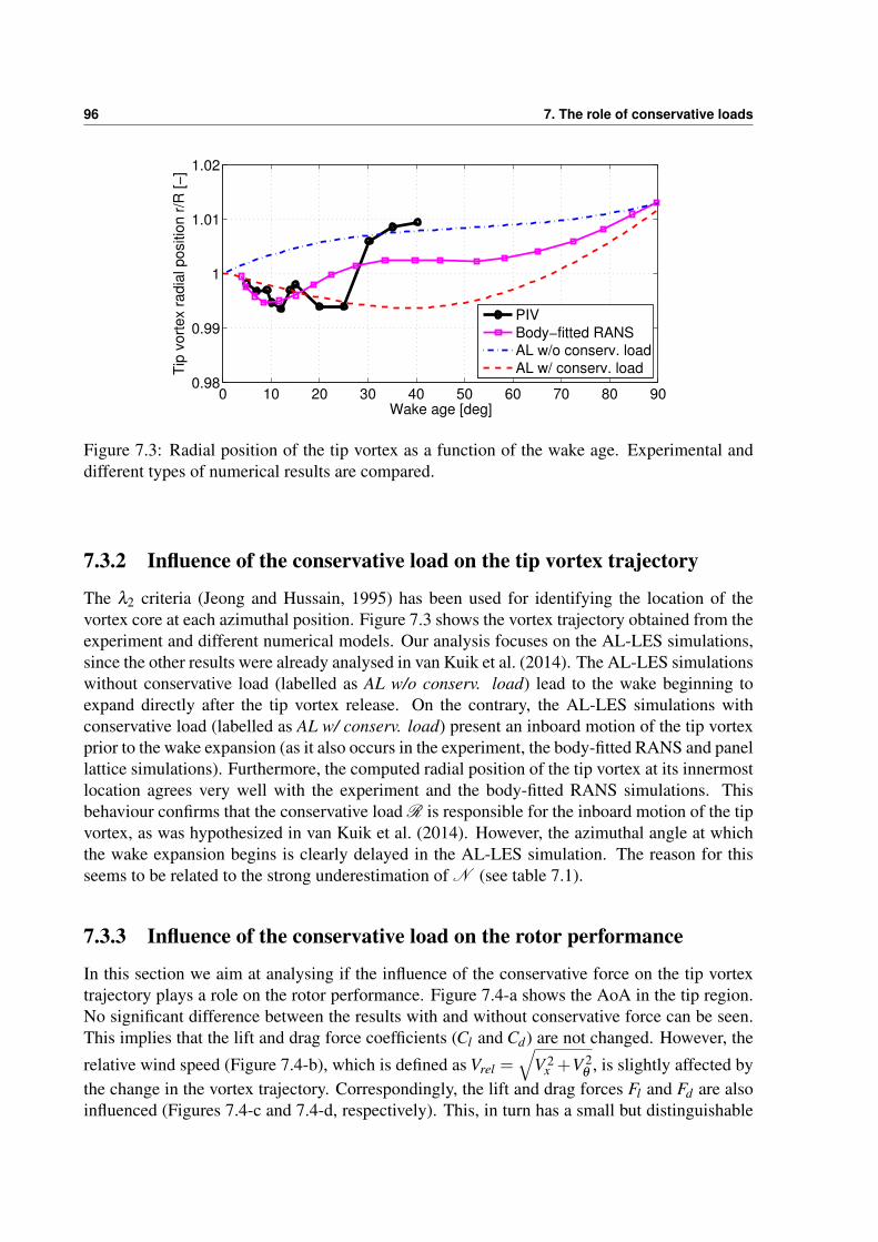
96 7. The role of conservative loads
0 10 20 30 40 50 60 70 80 900.98
0.99
1
1.01
1.02
Wake age [deg]
Tip
vort
ex r
adia
l positio
n r
/R [−
]
PIV
Body−fitted RANS
AL w/o conserv. load
AL w/ conserv. load
Figure 7.3: Radial position of the tip vortex as a function of the wake age. Experimental anddifferent types of numerical results are compared.
7.3.2 Influence of the conservative load on the tip vortex trajectory
The λ2 criteria (Jeong and Hussain, 1995) has been used for identifying the location of thevortex core at each azimuthal position. Figure 7.3 shows the vortex trajectory obtained from theexperiment and different numerical models. Our analysis focuses on the AL-LES simulations,since the other results were already analysed in van Kuik et al. (2014). The AL-LES simulationswithout conservative load (labelled as AL w/o conserv. load) lead to the wake beginning toexpand directly after the tip vortex release. On the contrary, the AL-LES simulations withconservative load (labelled as AL w/ conserv. load) present an inboard motion of the tip vortexprior to the wake expansion (as it also occurs in the experiment, the body-fitted RANS and panellattice simulations). Furthermore, the computed radial position of the tip vortex at its innermostlocation agrees very well with the experiment and the body-fitted RANS simulations. Thisbehaviour confirms that the conservative load R is responsible for the inboard motion of the tipvortex, as was hypothesized in van Kuik et al. (2014). However, the azimuthal angle at whichthe wake expansion begins is clearly delayed in the AL-LES simulation. The reason for thisseems to be related to the strong underestimation of N (see table 7.1).
7.3.3 Influence of the conservative load on the rotor performance
In this section we aim at analysing if the influence of the conservative force on the tip vortextrajectory plays a role on the rotor performance. Figure 7.4-a shows the AoA in the tip region.No significant difference between the results with and without conservative force can be seen.This implies that the lift and drag force coefficients (Cl and Cd) are not changed. However, the
relative wind speed (Figure 7.4-b), which is defined as Vrel =√
V 2x +V 2
θ, is slightly affected by
the change in the vortex trajectory. Correspondingly, the lift and drag forces Fl and Fd are alsoinfluenced (Figures 7.4-c and 7.4-d, respectively). This, in turn has a small but distinguishable

7.3 Results 97
effect on the driving torque and the thrust (Figures 7.4-e and 7.4-f, respectively). Integrating thetorque over the last 10% of the blade gives a difference of the torque at the tip with and withoutconservative load of approx. 2%. The total power of the turbine is reduced by approx. 1%.This contributes to mitigate the slight power overprediction of the simulation as compared tothe experiment (see Figure 7.1). This confirms that the conservative loads play an indirect roleon the rotor performance that should not be neglected if high order effects are to be considered.

98 7. The role of conservative loads
0
2
4
6
Ao
A [
de
g]
w/ conserv. load
w/o conserv. load6.2
6.4
6.6
6.8
7
7.2
7.4
V re
l /
V∞
[−
]
w/ conserv. load
w/o conserv. load
0
20
40
60
Fl [
N/m
]
w/ conserv. load
w/o conserv. load0
0.2
0.4
0.6
0.8
Fd [
N/m
]
w/ conserv. load
w/o conserv. load
0.9 0.95 10
1
2
3
4
r/R [−]
To
rqu
e [
Nm
/m]
w/ conserv. load
w/o conserv. load
0.9 0.95 10
20
40
60
r/R [−]
Th
rust
[N/m
]
w/ conserv. load
w/o conserv. load
(a) (b)
(c) (d)
(e) (f)
Figure 7.4: Influence of the conservative force on the spanwise distribution of (a) angle of attackAoA, (b) relative velocity Vrel , (c) sectional lift force Fl , (d) sectional drag force Fd , (e) sectionaltorque and (f) sectional thrust.

7.4 Conclusions 99
7.4 ConclusionsThe use of an enhanced actuator line model capable of applying conservative loads to the fluidallowed us to gain insight into the role of those loads on the rotor performance. The agreementof the model with experimental results and other numerical models representing the true geom-etry of the blade was in general satisfactory. However, the prediction of the radial wind velocitycomponent should be improved for obtaining a realistic normal component of the conservativeforce. The initial research questions have been successfully addressed:
• The conservative load acting on the chordwise bound circulation of a wind turbine bladeis confirmed to cause an inboard motion of the tip vortex after release and prior to thewake expansion.
• The influence of the conservative load on the tip vortex trajectory seems to play a small butnoticeable role on the power output. Its consideration helped to improve the consistencywith the experimental results. However, it must be kept in mind that this is a higherorder effect and correspondingly the numerical uncertainty might play a substantial role.Furthermore, the effect is assumed to be very dependent on the blade geometry.
• The consideration of conservative loads on tip loss correction models is recommended ifhigh order effects are to be considered.

100 7. The role of conservative loads

Chapter 8
Conclusions
This work has addressed the study of the aerodynamics of wind turbines by means of Computa-tional Fluid Dynamics (CFD) simulations. Special attention has been paid to the aerodynamicsof the blade root and tip regions, where the flow is highly three-dimensional and strongly influ-enced by the trailing vortices. The simulations of several wind turbines have been extensivelyvalidated against experimental results from model turbines operating under controlled condi-tions in a wind tunnel. The Reynolds Averaged Navier-Stokes (RANS) models were proven tobe suitable for the prediction of the flow around the blades and in the near wake. However, theaccuracy of this method was found to be reduced at stall conditions, since the models tendedto underpredict the flow separation. Large Eddy Simulations (LES) have also been performedwithin this thesis. However, their use was restricted to actuator line simulations, since the re-quired number of cells for solving the true blade geometry with boundary layer would be fartoo large for the available computational resources. The actuator line LES simulations wereespecially useful for the study of the tip vortex trajectory and evolution.
It has been shown that the blade inboard region is very prone to the presence of strongspanwise flows, especially in areas where the chordwise velocity is low. Furthermore, bothattached and separated flows can present significant radial flows. According to our results,the origin of these flows is not the existence of spanwise pressure gradients, as some authorshave suggested, but the centrifugal force acting on the boundary layer. The radial flows arealso affected by the Coriolis force, which “pushes” the flow towards the trailing edge. As aconsequence, the adverse pressure gradient on the suction side is reduced, what leads to thedelay of stall and the enhancement of lift. This phenomenon, which is known as Himmelskampeffect, did not play any significant role on the drag of the turbines studied in this thesis. Thisis in contrast to other wind turbines documented in the literature, where the drag was increasedor even reduced under the influence of the mentioned effect. The impact of the Himmelskampeffect on the Cp distribution seems to be very dependant on the airfoil geometry. The resultingCp distribution disparities between different airfoil types are not only quantitative, but alsoqualitative. This can be a major issue for the development of generalized correction models.
Another achievement of this thesis has been the correct prediction of trailing vortices in thetransition regions between airfoils of substantially different aerodynamic characteristics. As ithas been shown, those trailing vortices can disrupt the radial flows and correspondingly also theHimmelskamp effect. This is also a serious challenge for the development of reliable correctionmodels for this effect.

102 8. Conclusions
It has also been shown that the bound vorticity is oriented radially along most of the bladespan except at the tip and the root, where it is deflected towards the chordwise direction. Indeed,the chordwise bound vorticity is the origin of the tip and root trailing vortices. The changefrom spawise to chordwise bound vorticity is much more gradual at the root than at the tipand so are also the aerodynamic losses. This effect is most probably very dependant on theroot and tip geometry and it should be accounted for in the engineering correction models foraerodynamic losses. Another consequence of this effect is that the root vortex does not presenta well defined, distinctive structure. Furthermore, it has also been shown that the vortex trailedfrom the spanwise position of maximum chord length rotates in the opposite direction of theroot vortex. This explains the fast diffusion of the root vortex reported in many experiments.
The physical origin of the loads acting on the chordwise and the radial bound vorticity is thesame in both cases: pressure distributions on the blade surface. However, the load acting on theradial vorticity is orthogonal to the blade radius and the load acting on the chordwise vorticity isorthogonal to the blade chord. Hence, the load from the radial vorticity can produce work (i.e.contribute to the power conversion) and the load from the chordwise vorticity can not do it. Theformer is therefore a non-conservative load and the latter is a conservative load. Conservativeforces are always disregarded in the calculation methods based on the blade element theory(e.g. in blade element momentum and actuator line models). However, in this work an actuatorline model capable of computing and applying automatically the conservative load has beendeveloped. The comparison between simulations with and without conservative load allowedto conclude that the conservative load can modify the blade tip trajectory. Indeed, the existenceof that force explains the observations from several experiments, where the tip vortex presentsan inboard motion just after release from the blade tip and before the wake expansion drivesit outboard. The change in the tip vortex trajectory has been shown to influence slightly thepower conversion. Therefore, engineering models can be improved if the conservative tip loadis included. A similar effect is expected at the root. However, the relevance of this root effect isprobably negligible owing to the much stronger Himmelskamp effect and to the comparativelylow impact of the root forces on the power conversion.
These results show the great potential of CFD for the study of wind turbine aerodynamics.Furthermore, they pave the way for a better characterization of the blade flow. Ultimately, thisshould contribute to reduce the uncertainty in the design process of wind turbines and hence toimprove the cost-effectiveness of wind energy.

Chapter 9
Future work
This work has given insight into several aerodynamic phenomena affecting the blade tip androot of wind turbines by means of CFD simulations. Many of the limitations of the currentresults could be addressed in a future work:
• Use of Reynolds Stress Models (RSM) for modelling the turbulence: The turbulence mod-els used in this thesis are based on the Boussinesq approximation. One of the drawbacksof this method is the assumption of isotropic turbulence in the boundary layer. This is astrong simplification and in the case of highly three-dimensional flows it can affect thesimulation accuracy. Therefore, the use of more advanced Reynolds Stress Models isrecommended.
• Development of correction models: The final goal of the flow characterization is the im-plementation of reliable models. Hints and advices have been given for the developmentof correction models. This is however by no means a finished task and it should be con-tinued. There is still a long way to go until the physical mechanisms of the blade flow aresufficiently well understood for developing reliable corrections.
• Determination of the angle of attack: The determination of the angle of attack is oneof the main sources of uncertainty in the characterization of the blade aerodynamics.Further efforts should be performed for the development of reliable methods to computeand measure it.
• Sensitivity to blade geometry and airfoil type: the geometry of the tip and root as well asthe used airfoil type are expected to play a decisive role in the aerodynamic effects studiedin this thesis. The sensitivity to both factors should therefore be analysed in detail.
• Sensitivity to Reynolds number: the range of Reynolds number considered in this work isone order of magnitude lower than in full scale wind turbines. Therefore, its influence onthe studied effects should be analysed.
• Sensitivity to turbulence: all the results presented in this work were based on laminarinflow. This assumption was necessary for isolating the studied effects from other in-fluences and for validating the simulations against available wind tunnel measurements.However, full scale wind turbines operate under the influence of turbulence. Therefore,its role should be analysed.

104 9. Future work
• Other aspects of the root and tip flow: Many aspects of the tip and root flow deserve moreattention. As an example, the effect of the finite number of blades, the tip losses causedby the pressure equalization between the blade upper and lower sides, the interactionbetween root losses and Himmelskamp effect, the transition from laminar to turbulentflow, etc. should be studied in more depth.
• Transient aerodynamic effects: The study of transient aerodynamic effects was out of thescope of this thesis. However, they could be addressed in a future work. Examples ofsuch effects include dynamic stall, dynamic inflow, tower shadow, etc.

Bibliography
Akay, B., C. J. Ferreira, G. J. van Bussel, and I. Herraez2012a. Experimental and numerical quantification of radial flow in the root region of a hawt.In 50th AIAA Aerospace Sciences Meeting, Nashville, TN.
Akay, B., D. Micallef, C. J. Ferreira, and G. van Bussel2012b. Effects of geometry and tip speed ratio on the HAWT blade’s root flow. In Proceed-ings of the Science of Making Torque from Wind 2012, Oldenburg, Germany.
Akay, B., D. Ragni, C. Simao Ferreira, and G. van Bussel2014. Experimental investigation of the root flow in a horizontal axis wind turbine. WindEnergy, 17(7):1093–1109.
Bak, C., J. Johansen, and P. Andersen2006. Three–dimensional corrections of airfoil characteristics based on pressure distribu-tions. In 2006 European Wind Energy Conference Scientific Proceedings, Athens, Greece.
Banks, W. and G. Gadd1963. Delaying effect of rotation on laminar separation. AIAA Journal, 1(4):941–942.
Bechmann, A., N. N. Sørensen, and F. Zahle2011. CFD simulations of the MEXICO rotor. Wind Energy, 14(5):677–689.
Bertagnolio, F., N. Sørensen, J. Johansen, and P. Fuglsang2001. Wind turbine airfoil catalogue. Technical Report Risø–R–1280, Risø, Risø NationalLaboratory, Roskilde, Denmark.
Boorsma, K. and J. Schepers2003. Description of experimental setup. MEXICO measurements. Technical Report ECN–X–09–0XX, ECN, Petten, Netherlands.
Breton, S.-P., F. N. Coton, and G. Moe2008. A study on rotational effects and different stall delay models using a prescribed wakevortex scheme and NREL phase VI experiment data. Wind Energy, 11(5):459–482.
Carrion, M., M. Woodgate, R. Steijl, G. Barakos, S. Gomez-Iradi, and X.Munduate2012. Cfd and aeroelastic analysis of the mexico wind turbine. In Proceedings of the Scienceof Making Torque from Wind 2012, Oldenburg, Germany.

106 Bibliography
Chaviaropoulos, P. K. and M. O. L. Hansen2000. Investigating three–dimensional and rotational effects on wind turbine blades by meansof a quasi–3D Navier-Stokes solver. Journal of Fluids Engineering, 122(2):330–336.
Constantinides, Y. and O. Oakley2006. Numerical prediction of bare and straked cylinder VIV. In Proceedings from 25th Inter-national Conference on Offshore Mechanics and Arctic Engineering, OMAE2006, Hamburg,Germany.
Conway, J. T.1998. Exact actuator disc solutions for non-uniform heavy loading and slipstream contrac-tion. Journal Fluid Mechanics, 365:235–267.
Corrigan, J. and H. Schillings1994. Empirical model for stall delay due to rotation. In Proceedings of the AmericanHelicopter Society Aeromechanics Specialists Conference 1994, San Francisco, CA.
Corten, G.2001. Flow Separation on Wind Turbine Blades. PhD thesis, University of Utrecht.
de Villiers, E.2006. The Potential of Large Eddy Simulation for the Modelling of Wall Bounded Flows.PhD thesis, Imperial College London.
del Campo, V., D. Ragni, D. Micallef, B. Akay, F. J. Diez, and C. S. Ferreira2014. 3D load estimation on a horizontal axis wind turbine using SPIV. Wind Energy,17(11):1645–1657.
Drzewiecki, S.1892. Bulletin de L’Association Technique Maritime, Paris.
Du, Z. and M. Selig1998. A 3D stall-delay model for horizontal axis wind turbine prediction. In Proceedings of1998 ASME Wind Energy Symposium, number AIAA-98-0021, Reno, NV, USA.
Du, Z. and M. Selig2000. The effect of rotation on the boundary layer of a wind turbine blade. RenewableEnergy, 20(2):167 – 181.
Dumitrescu, H. and V. Cardos2004. Rotational effects on the boundary-layer flow in wind turbines. AIAA Journal,42(2):408–411.
Duque, E. P. N., M. D. Burklund, and W. Johnson2003. Navier-Stokes and comprehensive analysis performance predictions of the NRELPhase VI experiment. Journal of Solar Energy Engineering, 125(4):457–467.

Bibliography 107
Duque, E. P. N., C. van Dam, and S. Hughes1999. Navier-Stokes simulations of the NREL combined experiment Phase II rotor. In Pro-ceedings 1999 ASME Wind Energy Symposium, number AIAA-99-0037, Pp. 143–153, Reno,NV.
Ebert, P. and D. Wood2001. The near wake of a model horizontal–axis wind turbine: Part 3: properties of the tipand hub vortices. Renewable Energy, 22(4):461 – 472.
Ferrer, E. and X. Munduate2007. Wind turbine blade tip comparison using cfd. Journal of Physics: Conference Series,75(012005).
Ferziger, J. and M. Peric2002. Computational methods for fluid dynamics. Springer.
FLOW2015. Facility for Large-scale COmputations in Wind Energy Research. http://www.fk5.uni-oldenburg.de/57249.html. Accessed: October 2015.
Froude, R.1889. On the part played in propulsion by differences of fluid pressure. Transactions Instituteof Naval Architects, 30:390–405.
Froude, W.1878. Transactions Institute of Naval Architects, 19:47.
Germano, M., U. Piomelli, and P. W. Cabot1991. A dynamic subgrid-scale eddy viscosity model. Physics of Fluids A, 3(7):1760–1765.
Glauert, H.1935. The general momentum theory. In Aerodynamic Theory, W. Durand, ed., volume IV.Division L. Springer. Reprinted 1963 Dover.
Guntur, S., C. Bak, and N. Sørensen2011. Analysis of 3D stall models for wind turbine blades using data from the MEXICOexperiment. In Proceedings of 13th International Conference on Wind Engineering, Amster-dam, The Netherlands.
Guntur, S. and N. Sørensen2012. An evaluation of several methods of determining the local angle of attack on windturbine blades. In Proceedings of the Science of Making Torque from Wind 2012, Oldenburg,Germany.
Guntur, S. and N. N. Sørensen2014. A study on rotational augmentation using cfd analysis of flow in the inboard region ofthe mexico rotor blades. Wind Energy.

108 Bibliography
Haans, W., G. van Kuik, and G. van Bussel2008. The inverse vortex wake model:a measurement analysis tool. Journal of Solar EnergyEngineering, 130(3):031009–031009–14.
Hand, M., D. Simms, L. Fingersh, D. Jager, J. Cotrell, S. Schreck, and S. Larwood2011. Unsteady aerodynamics experiment phase vi: wind tunnel test configurations andavailable data campaigns. Technical Report NREL/TP-500-29955, Risø, National RenewableLaboratory.
Hansen, M., N. Sørensen, J. Sørensen, and J. Michelsen1997. Extraction of lift, drag and angle of attack from computed 3D viscous flow around arotating blade. In Scientific Proceedings from European Wind Energy Conference, EWEC’97,Pp. 499–501, Dublin, Ireland.
Hansen, M. L. and H. Aagaard Madsen2011. Review paper on wind turbine aerodynamics. Journal of Fluids Engineering,133(11):114001–114001–12.
Herraez, I., B. Stoevesandt, and J. Peinke2014. Insight into rotational effects on a wind turbine blade using Navier–Stokes computa-tions. Energies, 7(10):6798–6822.
Himmelskamp, H.1947. Profile investigations on a rotating airscrew, Reports and translations. VolkenrodeMAP.
Issa, R. I.1985. Solution of the implicitly discretized fluid flow equations by operator-splitting. Journalof Computational Physics, 62:40–65.
Ivanell, S., J. Sørensen, R. Mikkelsen, and D. Henningson2007. Numerical analysis of the tip and root vortex position in the wake of a wind turbine.Journal of Physics: Conference Series, 75(012035).
Ivanell, S., J. N. Sørensen, R. Mikkelsen, and D. Henningson2009. Analysis of numerically generated wake structures. Wind Energy, 12(1):63–80.
Jeong, J. and F. Hussain1995. On the identification of a vortex. Journal of Fluid Mechanics, 285:69–94.
Jha, P. K., M. J. Churchfield, P. J. Moriarty, and S. Schmitz2014. Guidelines for volume force distributions within actuator line modeling of wind tur-bines on Large-Eddy Simulation-type grids. J. Sol. Energy Eng., 136(3):031003–031003–11.
Jin, W.2013. Numerical simulation of wind turbine wakes based on actuator line method inNEK5000. Master’s thesis, KTH, Sweden.

Bibliography 109
Johansen, J. and N. N. Sørensen2004. Aerofoil characteristics from 3D CFD rotor computations. Wind Energy, 7(4):283–294.
Johansen, J., N. N. Sørensen, J. A. Michelsen, and S. Schreck2002. Detached-eddy simulation of flow around the NREL Phase VI blade. Wind Energy,5(2-3):185–197.
Jonkman, J., S. Butterfield, W. Musial, and G. Scott2009. Definition of a 5 mw reference wind turbine for offshore system development. Tech-nical Report NREL/TP-500-38060, NREL, Golden, CO, USA.
Kwon, S., J. Cho, J. Park, and H. Choi2002. The effects of drag reduction by ribbons attached to cylindrical pipes. Ocean Engi-neering, 29(15):1945–1958.
Laizet, S. and J. C. Vassilicos2011. Dns of fractal generated turbulence. Flow, turbulence and combustion, 87:673–705.
Launder, B., G. Reece, and W. Rodi1975. Progress in the development of a Reynolds stress turbulence closure. Journal of FluidMechanics, 68:537–566.
Launder, B. and D. Spalding1974. The numerical computation of turbulent flows. Computer Methods in Applied Me-chanics and Engineering, 3:269–289.
Le Pape, A. and J. Lecanu2004. 3D Navier–Stokes computations of a stall–regulated wind turbine. Wind Energy,7(4):309–324.
Leishman, J. G.2002. Challenges in modelling the unsteady aerodynamics of wind turbines. Wind Energy,5(2-3):85–132.
Lilly, D. K.1967. The representation of small–scale turbulence in numerical simulation experiments. InProc. IBM Scientific Computing Symposium on Environmental Sciences.
Lindenburg, C.2003. Investigation into rotor blade aerodynamics. Technical Report ECN-C03-025, ECN,Petten, Netherlands.
Massouh, F. and I. Dobrev2007. Exploration of the vortex wake behind of wind turbine rotor. Journal of Physics:Conference Series, 75(012036).
McCroskey, W. and P. Yaggy1968. Laminar boundary layers on helicopter rotors in forward flight. AIAA Journal,6(10):1919–1926.

110 Bibliography
Medici, D. and P. H. Alfredsson2006. Measurements on a wind turbine wake: 3D effects and bluff body vortex shedding.Wind Energy, 9(3):219–236.
Menter, F.1993. Zonal two equation k–ω turbulence models for aerodynamic flows. AIAA Journal,93(2906).
Menter, F.1994. Two–equation eddy-viscosity turbulence models for engineering applications. AIAAJournal, 32(8):1598–1605.
Micallef, D.2012. 3D flows near a HAWT rotor: A dissection of blade and wake contributions. PhDthesis, Delft University of Technology.
Micallef, D., B. Akay, C. S. ao Ferreira, T. Sant, and G. van Bussel2012. The origins of a wind turbine tip vortex. In Proceedings of the Science of MakingTorque from Wind 2012, Oldenburg, Germany.
Micallef, D., G. van Bussel, C. S. a. Ferreira, and T. Sant2013. An investigation of radial velocities for a horizontal axis wind turbine in axial andyawed flows. Wind Energy, 16(4):529–544.
Mockett, C.2009. A comprehensive study of detached-eddy simulation. PhD thesis, Technical Universityof Berlin.
Nilsson, K., W. Z. Shen, J. N. Sørensen, S. P. Breton, and S. Ivanell2015a. Validation of the actuator line method using near wake measurements of the MEXICOrotor. Wind Energy, 18(3):499–514.
Nilsson, K., W. Z. Shen, J. N. Sørensen, S.-P. Breton, and S. Ivanell2015b. Validation of the actuator line method using near wake measurements of the mexicorotor. Wind Energy, 18(9):1683–1683.
Okulov, V. L., J. N. Sørensen, and D. H. Wood2015. The rotor theories by Professor Joukowsky: Vortex theories. Progress in AerospaceSciences, Pp. 19–46.
OpenFOAM2015. OpenFOAM: the open source CFD toolbox. www.openfoam.com. Accessed: October2015.
Pascal, L.2009. Analysis of MEXICO Measurements. Technical Report ECN-Wind Memo-09-010,ECN, Petten, Netherlands.

Bibliography 111
Patankar, S. V.1980. Numerical Heat Transfer and Fluid Flow. Taylor & Francis.
Pointwise2015. Pointwise. www.pointwise.com. Accessed: October 2015.
Pope, S. B.2000. Turbulent flows. Cambridge University Press.
Raj, N.2000. An improved semi–empirical model for 3D post–stall effects in horizontal axis windturbines. Master’s thesis, University of Illinois, Urbana–Champaign.
Rankine, W. J. M.1865. On the mechanical principles of the action of propellers. Transactions Institute ofNaval Architects, 6:13–39.
Rethore, M., F. Zahle, N. Sørensen, and A. Bechmann2011. CFD simulations of the mexico wind tunnel and wind turbine. In Proceedings ofEWEA 2011, Brussels, Belgium.
Roache, P. J.1994. Perspective: A method for uniform reporting of grid refinement studies. Journal ofFluids Engineering, 116(3):405.
Roache, P. J.1998a. Perspective: A Method for Uniform Reporting of Grid Refinement Studies, Pp. 8–9.Hermosa Publishers.
Roache, P. J.1998b. Perspective: A Method for Uniform Reporting of Grid Refinement Studies, Pp. 8–9.Hermosa Publishers.
Robinson, M., M. Hand, S. Simms, and S. Schreck1999. Horizontal axis wind turbine aerodynamics: Three–dimensional, unsteady, and sepa-rated flow influences. In Proceedings of FEDSM99, number FEDSM99-S295-01, San Fran-cisco, CA.
Ronsten, G.1992. Static pressure measurements on a rotating and a non-rotating 2.375 m wind turbineblade. comparison with 2D calculations. Journal of Wind Engineering and Industrial Aero-dynamics, 39(1–3):105–118.
Rung, T., H. Lubcke, and F. Thiele2001. Universal wall-boundary conditions for turbulence-transport models. ZAMM - Jour-nal of Applied Mathematics and Mechanics / Zeitschrift fur Angewandte Mathematik undMechanik, 81(S3):481–482.

112 Bibliography
Schepers, J.2012. Engineering models in wind energy aerodynamics. PhD thesis, TU-Delft.
Schepers, J., K. Boorsma, T. Cho, S. Gomez-Iradi, A. Schaffarczyk, A. Jeromin, W. Shen,T. Lutz, K. Meister, B. Stoevesandt, S. Schreck, D. Micallef, R. Pereira, T. Sant, H. Madsen,and N. Sørensen2012. Final report of iea task 29, mexnext (phase 1): Analysis of mexico wind tunnel mea-surements. Technical Report ECN–E–12–004, ECN, KARI, CENER, CEWind EG, DTU,University of Stuttgart, ForWind, NREL, TUDelft, RISØ.
Schepers, J., K. Boorsma, C. Kim, and T. Cho2011. Analysis of detailed aerodynamic measurements on a 4.5 m diameter rotor placed in thelarge german dutch wind tunnel DNW. In Proceedings of EWEA 2011, Brussels, Belgium.
Schepers, J. and H. Snel2007. Model experiments in controlled conditions, final report. Technical Report ECN-E-07-042, ECN, Petten, Netherlands.
Schmidt, T., C. Mockett, and F. Thiele2009. Adaptive wall function for the prediction of turbulent flows. In MEGADESIGN andMegaOpt - German Initiatives for Aerodynamic Simulation and Optimization in Aircraft De-sign, N. Kroll, D. Schwamborn, K. Becker, H. Rieger, and F. Thiele, eds., volume 107 ofNotes on Numerical Fluid Mechanics and Multidisciplinary Design, Pp. 21–33. SpringerBerlin Heidelberg.
Schreck, S. and M. Robinson2002. Rotational augmentation of horizontal axis wind turbine blade aerodynamic response.Wind Energy, 5(2-3):133–150.
Schreck, S., T. Sant, and D. Micallef2010. Rotational augmentation disparities in the mexico and UAE phase vi experiments. InProceedings of the Science of Making Torque from Wind 2010, Heraklion, Crete, Greece.
Schreck, S. J., N. N. Sørensen, and M. C. Robinson2007. Aerodynamic structures and processes in rotationally augmented flow fields. WindEnergy, 10(2):159–178.
Shen, W. Z., M. O. L. Hansen, and J. N. Sørensen2009. Determination of the angle of attack on rotor blades. Wind Energy, 12(1):91–98.
Shen, W. Z., J. N. Sørensen, and R. Mikkelsen2005. Tip loss correction for actuator/Navier–Stokes computations. Journal of Solar Engi-neering, 127:209–213.
Shen, W. Z., W. J. Zhu, and J. N. Sørensen2012. Actuator line/Navier–Stokes computations for the MEXICO rotor: comparison withdetailed measurements. Wind Energy, 15(5):811–825.

Bibliography 113
Sherry, M., J. Sheridan, and D. Jacono2013. Characterisation of a horizontal axis wind turbine’s tip and root vortices. Experimentsin Fluids, 54(3).
Shives, M. and C. Crawford2013. Mesh and load distribution requirements for actuator line CFD simulations. WindEnergy, 16(8):1183–1196.
Sicot, C., P. Devinant, S. Loyer, and J. Hureau2008. Rotational and turbulence effects on a wind turbine blade. investigation of the stallmechanisms. Journal of Wind Engineering and Industrial Aerodynamics, 96(8–9):1320–1331.
Simms, D., S. Schreck, and L. Fingeresh2001. NREL unsteady aerodynamics experiment in the NASA–Ames wind tunnel: a com-parison of predictions to measurements. Technical Report NREL/TP–500–29494, NationalRenewable Energy Laboratory, Golden, CO, USA.
Smagorinsky, J.1963. General circulation experiments with the primitive equations. Monthly Weather Re-view, 91:99–164.
Snel, H., R. Houwink, G. van Bussel, and A. Bruining1993. Sectional prediction of 3D effects for stalled flow on rotating blades and comparisonwith measurements. In 1993 European Community Wind Energy Conference Proceedings,Pp. 395–399, Travemunde, Germany.
Sørensen, J. and W. Shen2002. Numerical modelling of wind turbine wakes. Journal of Fluids Engineering,124(2):393–399.
Sørensen, J. N.2015. General Momentum Theory for Horizontal Axis Wind Turbines. Springer.
Sørensen, N. and S. Schreck2012. Computation of the National Renewable Energy Laboratory Phase–VI rotor in pitchmotion during standstill. Wind Energy, 15(3):425–442.
Sørensen, N. N., A. Bechmann, P. E. Rethore, and F. Zahle2014. Near wake Reynolds-averaged Navier—Stokes predictions of the wake behind theMEXICO rotor in axial and yawed flow conditions. Wind Energy, 17(1):75–86.
Sørensen, N. N., J. A. Michelsen, and S. Schreck2002. Navier–Stokes predictions of the NREL phase VI rotor in the NASA Ames 80 ft x 120ft wind tunnel. Wind Energy, 5(2-3):151–169.
SOWFA2015. SOWFA: Simulator for wind farm applications. https://nwtc.nrel.gov/SOWFA. Ac-cessed: October 2015.

114 Bibliography
Spalart, P.2000. Strategies for turbulence modelling and simulation. International Journal for Heatand Fluid Flow, 21(3):252–263.
Spalart, P., W.-H. Jou, M. Strelets, and S. Allmaras1997. Comments on the feasibility of LES for wings, and on a hybrid RANS/LES approach.In Advances in LES/DNS, First AFOSR International Conference on DNS/LES, GreydenPress, Louisiana Tech University.
Spalart, P. R. and S. R. Allmaras1994. A one-equation turbulence model for aerodynamic flows. La Recherche Aerospatiale,1(1):5–21.
Spalding, D. B.1961. A single formula for the law of the wall. Journal of Applied Mechanics, 28(3):444–458.
Tangler, J. and M. Selig1997. An evaluation of an empirical model for stall delay due to rotation for HAWTs. InProceedings of WindPower 97, Austin, Texas.
Tangler, J. L.2004. Insight into wind turbine stall and post–stall aerodynamics. Wind Energy, 7(3):247–260.
Troldborg, N.2008. Actuator Line Modeling of Wind Turbine Wakes. PhD thesis, Technical University ofDenmark.
Troldborg, N., C. Bak, N. Sørensen, H. Madsen, M. Rethore, F. Zahle, and S. Guntur2013. Experimental and numerical investigation of 3D aerofoil characteristics on a MW windturbine. In Proceedings of EWEA 2013, Vienna, Austria.
Troldborg, N., J. N. Sørensen, and R. Mikkelsen2007. Actuator line simulation of wake of wind turbine operating in turbulent inflow. InProceedings of the Science of Making Torque from Wind 2007, Copenhagen, Denmark.
van Kuik, G.1991. On the limitations of Froude’s actuator disc concept. PhD thesis, Technical UniversityEindhoven, The Netherlands.
van Kuik, G. A. M., D. Micallef, I. Herraez, A. H. van Zuijlen, and D. Ragni2014. The role of conservative forces in rotor aerodynamics. Journal of Fluid Mechanics,750:284–315.
van Kuik, G. A. M., J. N. Sørensen, and V. L. Okulov2015. Rotor theories by Professor Joukowsky: Momentum theories. Progress in AerospaceSciences, 73:1–18.

Bibliography 115
Vermeer, L., J. Sørensen, and A. Crespo2003. Wind turbine wake aerodynamics. Progress in Aerospace Sciences, 39(6-7):467–510.
Versteeg, H. and W. Malalasekera1995. An Introduction to Computational Fluid Dynamics. Pearson Prentice Hall.
Wald, Q. R.2006. The aerodynamics of propellers. Progress in Aerospace Sciences, 42(2):85–128.
Wilcox, D. C.1998. Turbulence Modelling for CFD. DCW Industries.
Wood, D.1991. A three-dimensional analysis of stall–delay on a horizontal–axis wind turbine. Journalof Wind Engineering and Industrial Aerodynamics, 37(1):1–14.
Wu, Y. T. and F. Porte-Agel2010. Large-Eddy simulation of wind-turbine wakes: Evaluation of turbine parametrisations.Boundary-Layer Meteorol, 138:345–366.
Xiao, J., J. Wu, L. Chen, and Z. Shi2011. Particle image velocimetry (PIV) measurements of tip vortex wake structure of windturbine. Appl. Math. Mech., 32(6):729—738.

116 Bibliography

List of publications 117
Publications on which this thesis is based:
Peer-reviewed publications
I. HERRAEZ, W. MEDJROUBI, B. STOEVESANDT AND J. PEINKE, Aerodynamic Simulationof the MEXICO Rotor, Journal of Physics: Conference Series, 555, 012051, 2014.
I. Herraez performed the simulations, carried out the scientific analysis and wrote themanuscript. W. Medjroubi, B. Stoevesandt and J. Peinke had a supervising function.
I. HERRAEZ, B. STOEVESANDT AND J. PEINKE, Insight into Rotational Effects on a WindTurbine Blade Using Navier-Stokes Computations, Energies, 7, 6798-6822, 2014.
I. Herraez performed the simulations, carried out the scientific analysis and wrote themanuscript. B. Stoevesandt and J. Peinke had a supervising function.
P. LIND, I. HERRAEZ, M. WACHTER AND J. PEINKE, Fatigue Load Estimation through aSimple Stochastic Model, Energies, 7, 8279, 2014.
The original idea of the article is from J. Peinke. P. Lind implemented the stochasticmodel and wrote the manuscript. I. Herraez carried out the fatigue load analysis. M.Wachter and J. Peinke had a supervising function.
G.A.M. VAN KUIK, D. MICALLEF, I. HERRAEZ, A.H. VAN ZUJLEN AND D. RAGNI, Therole of conservative forces in rotor aerodynamics, Journal of Fluid Mechanics, 750, 284-315, 2014.
G.A.M. van Kuik proposed the main ideas of the paper. He also performed the analyticalwork and wrote the article. D. Micallef did the measurements and carried out panel codesimulations. I. Herraez performed Navier-Stokes simulations based on the true bladegeometry and on an actuator line model. A.H. van Zujlen contributed with actuator disksimulations. D. Ragni supported the experimental work.
I. HERRAEZ, B. AKAY, G.J.W. VAN BUSSEL, J. PEINKE AND B. STOEVESANDT, DetailedAnalysis of the Blade Root Flow of a Horizontal Axis Wind Turbine, Wind Energy Sci-ence, in review.
I. Herraez performed the simulations, carried out most of the scientific analysis and wrotethe manuscript. B. Akay provided the experimental results. G.J.W. van Bussel contributedto the analysis of the measurements. J. Peinke and B. Stoevesandt had a supervisingfunction.
I. HERRAEZ, D. MICALLEF, G.A.M. VAN KUIK AND J. PEINKE, Numerical evidence of theinfluence of conservative forces on the performance of rotor blades, Wind Energy Science,in review.
I. Herraez performed the simulations, analysed the results and wrote the manuscript. D.Micallef and G.A.M. van Kuik contributed to the interpretation of the results. J. Peinkehad a supervising function.

118 List of publications
D. TRAPHAN, I. HERRAEZ, P. MEINLSCHMIDT, F. SCHLUTER, J. PEINKE AND G.GULKER, Remote surface damage detection on rotor blades of operating wind turbinesby means of infrared thermography, in preparation to be submitted to Applied Energy.
D. Traphan carried out the measurements and wrote the manuscript. I. Herraez performedthe simulations. The scientific analysis was done by D. Traphan and I. Herraez. P.Meinlschmidt and F. Schluter contributed to the experimental work. J. Peinke and G.Gulker had a supervising function.
Book chapters
E. DANIELE, I. HERRAEZ, B. STOEVESANDT AND J. PEINKE, DES study of airfoil liftcoefficient sensitivity to flow turbulence, Wind Energy - Impact of turbulence, editors M.Holling, J. Peinke and S. Ivanell, Springer Berlin Heidelberg, 2014.
Conference proceedings
B. AKAY, C. S. FERREIRA, G.J.W. VAN BUSSEL AND I. HERRAEZ, Experimental and nu-merical quantification of the flow in the root region of a HAWT, Proceedings of the 50thAIAA Aerospace Sciences Meeting, Nashville, Tennessee, 2012.
I. HERRAEZ, B. STOEVESANDT AND J. PEINKE, Validating OpenFOAM with the MEXICODataset, Proceedings of the 7th EAWE PhD Seminar on Wind Energy in Europe, Delft,the Netherlands, 2011.
I. HERRAEZ, B. STOEVESANDT AND J. PEINKE, Numerical Study of Rotational Effects onWind Turbines, Proceedings of the DEWEK 2015, Bremen, 2015.

Acknowledgments 119
Acknowledgments
Working on this thesis has been an enjoyable and rewarding adventure thanks to many peo-ple who supported me in one way or the other.
I would like to express my sincere gratitude to Prof. Joachim Peinke for advising me, placinghis trust and confidence in my work and giving me a lot of freedom for following my owninterests and ideas. Many thanks to Bernhard Stoevesandt for his support and helping me todevelop my background in the field of CFD. I am also very grateful to Wided Medjroubi for herguidance and encouragement in the first stage of the PhD. I thank Prof. Martin Kuhn for willingto be part of the defence committee of this thesis.
Many thanks to my collaborators from the TU-Delft: I am specially grateful to Prof. GijsA.M. van Kuik , with whom I had the privilege to cooperate during his research stay at theUniversity of Oldenburg (and afterwards). He gave me a new perspective for my research andI really enjoyed each of our (not only scientific) discussions. I also would like to thank Prof.Gerard J.W. van Bussel for his insightful and motivating comments about our common work.I am grateful to Busra Akay for sharing her experimental work with me and for the fruitfulcollaboration. Thanks a lot too to Daniel Micallef, from whom I learned much in our commonarticles.
I would like to express my gratitude to the participants of the MexNext-project for theinsightful meetings and discussions.
I thank Stefan Albensoeder for his support with the computer cluster of the University ofOldenburg and for his kind help with any kind of IT problems. I am also very grateful to mycolleges from the CFD group Hamid Rahimi, Bastian Dose, Lena Vorspel, Sebastian Ehrich,Michael Schwarz, Elia Daniele, Jose Parra, Jonas Schmidt, Carlos Peralta, Matthias Schramm,Samuel Chang, and Cherif Mihoubi for the relaxed and friendly working atmosphere. Manythanks also to other colleges of the TWiSt and We-Sys groups including Philip Rinn, MatthiasWachter, Mike Holling, Patrick Milan, Gerd Gulker, Jannik Schottler, Nico Reinke, Jarek Puczy-lowski, Stanislav Rockel, Alan Morales, Luis Vera-Tudela, Juan Jose Trujillo and many othersthat contributed to make my stay at the University of Oldenburg an unforgettable experience.Special thanks to Dominik Traphan and Pedro Lind for the enjoyable cooperations within ourresearch group. I would like to extend my sincere gratitude also to George Pechlivanoglou, whoencouraged me to do this PhD.
I am very grateful to my parents and sister as well as to Herena for their continuous supportnot only during this thesis, but always. Last but no least, my deepest thankfulness goes to mydaughters Zoe and Yara, who had to share their dad too often with this thesis.

120 Acknowledgments

Curriculum vitae 121
Curriculum vitae
Personal data:Name Ivan Herraez Hernadez
Date of birth 30.01.1979
Place of birth Barcelona (Spain)
Nationality Spanish
Education:10/2010 – 12/2015 Doctoral student under the supervision of Prof. Dr.
Peinke at University of Oldenburg, Germany
10/2005 – 04/2007 M.Sc. Renewable Energy at the University ofOldenburg, Germany.
10/1998 – 08/2002 B.Sc. Mechanical Engineering at the University ofLeon, Spain. Exchange student at the FH-Ulm(WS00-01/SS01)and the RWTH-Aachen (WS01-02/SS02)
Professional experience:
10/2014 – present Leader of the subgroup “CFD” in the research groupof Prof. Dr. Peinke at the University of Oldenburg,Germany
05/2007 – 09/2010 Development engineer at the company Nordex GmbH.Load calculation and structural-dynamic analysis ofwind turbines.

Erklarung
Ich erklare hiermit, dass ich diese Arbeit selbststandig verfasst und nur die angegebenenHilfsmittel benutzt habe.
Oldenburg, den 04. Januar 2016
......................................................................................
(Ivan Herraez Hernadez)


