AD-785 623

ON THE ARITHMETIC MEANS AND VARIANCESOF PRODUCTS AND RATIOS OF RANDOMVARIABLES

Fred Frishman

Army Research OfficeDurham, North Carolina

1971

DISTRIBUTED BY:

National Technical Idmtio SerieU. S. DEPARTMENT OF COMMERCE5285 Port Royal Road, Springfield Va. 22151

iJ----n II-

FRISHMAN AD 785 623

1ON THE ARITHMETIC MEANS AND VARIANCES OFPRODUCTS AND RATIOS OF RANDOM VARIABLES

tie FRED FRISHMAN, DR.

U. S. ARMY RESEARCH OFFICEgot DURHAM, NORTH CAROLINA

I *_

1. INTRODUCTION

In the sciences and other disciplines, it is quite common toencounter situations where random variables appear in combinations.Two combinations are the product and the ratio of two random vai-ables. Given such combinations, it is required to know the mean and

- -, the variance and it is preferable that the mean and variance be deter-mined from the original random variables. Thus, if U = XY andV = X/Y then we want to know the arithmetic means and variances of Uand V based on our knowledge of X and Y.

2. ON THE PRODUCT OF TWO RANDOM VARIABLESThe mean and the variance of a product are well known [ 5.

To obtain the result in a more simple manner, we note that

(2.1) Cov(X,Y) = E(XY) - E(X) E(Y)

provided that the moments exist. Henceforth, we will assume that themoments exist.

By rearranging (2.1), we obtain

(2.2) E(XY) = Cov(X,Y) + E(X) E(Y).

Further, the definition of the linear correlation coefficient PX,Y is

given by(.)CoV(X, Y)(2.3) PXY 1 VrX]/2[Vr 1)]/2

- Var(X)] 1,'a[(Y)] /

f4ATIONAl TFCHNICALINFORMATION SERVICE"U S D,'p.,,-wnF o Co-mrre' 331

"p;i nt'+, If ',A 'I VA

- - l" |- " I l , . . ',,H # ' J , ' - '' ' '' :

'- '-' J ' ' ' ' %" "''= .. . .. . . . " ...'

FRISHMAN

By introducing (2.3) into (2.2), it is seen that

(2.4) E (XY)=E M)E (Y) + pX Y~(Var(X) 1 12(Var(Y) 1 1/2a

To obtain the variance of a product of random variables, wenote that

(2.5) VartOCY= E( XIY )-E(XY)]

and that

(2.6) Cov(X2 ,Y2 ) =E (X2Y2 )-E (X2 )E(Y2

Then from (2.1) and (2.5),2 2 X2) 2Cov (X , Y2) = Var (XY) + (Cov (X, Y) + E(M)E(Y)1 - E( )E(Y2

2-Var(XY) +(Cov (X,Y)1 +2 Cov(X,Y) E(X)E(Y)

-Var (X) Var (Y) - Var (X) C F(Y)1 Var(Y) [E(X)12

Then, by rearrangement of terms,

(2.7) Var(XY) =Cov(X 2Y )-f2Cov(XY) 1 -_2 Cov(X, Y) E ()E(Y)2 2+ Var(XM Var (Y) + VarX)I(E (Y) I + Var (Y) E E X) I

If X and Y are independent or uncorrelated, (2 .2)and (2.7) reduce to

(2,8) E(XY) =E(X) E(Y),

and

(2.9) Var(XY) =Var(X)Var(Y) +Var(X)[E(Y)1 +Var(Y)(E(X)1In addition, if the two variables are independent or uncorrelated, then

(2.10) Var(XY) = Var(X) Var(Y)

only if the means of both random variables are zero.

3. ONE SET OF RESULTS FOR THE MEAN AND VARIANCE OF A RATIO_OF" RANDOM VARIABLES

We can write, using (2.3) E(-I~)- E (Y) Ei)

Then as in (2.4),

(3.2) E Y E(Y) E rJ+ p ~Var(Y) 1/ Vark x)1/2

332

- - - - - - - - - - -_ _ _ _ _ _ _ _ _ _

)FRISHMAN

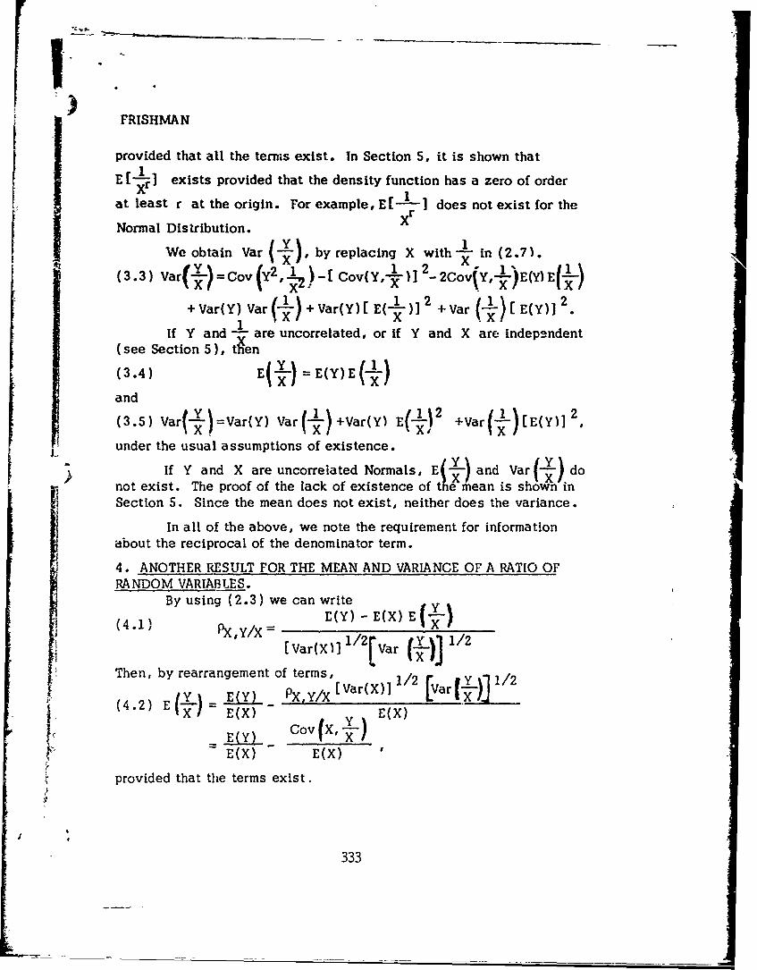
provided that all the terms exist. In Section 5, it is shown that

E[--1 exists provided that the density function has a zero of order

at least r at the origin. For example, E[ - does not exist for theNormal Distribution. xI Y elcn wthj in ( 2.7 ).We obtain Var (-fl,o by replacing Xwih-i n(27

+ aar)[ (_j) 22

Var(Y) 1 VrEY

If Y and - are uncorrelated, or if Y and X are indep2ndent(see Section 5), t~en

and

under the usual assumptions of existence.

If Y and X are uncorrelated Normals, E -Y-) and. Var (1 - donot exist. The proof of the lack of existence of the mean is shown inSection 5. Since the mean does not exist, neither does the variance.

In all of the above, we note the requirement for informationabout the reciprocal of the denominator term.

4. ANOTHER RESULT FOR THE MEAN AND VARIANCE OF A RATIO OFRANDOM VARIABLES.

By using (2.3) we can write

(4.1)PX, Y/X =[Var(X)] 1/2 Var (i_)] 1/2

Then, by rearrangement of terms, 1/2 1/2

(4.2) E E(Y) - PXY/X war(x) ] 1 ar

E(Y) - EE(X) E(X)

provided that the terms exist,j

333

FRISHMAN

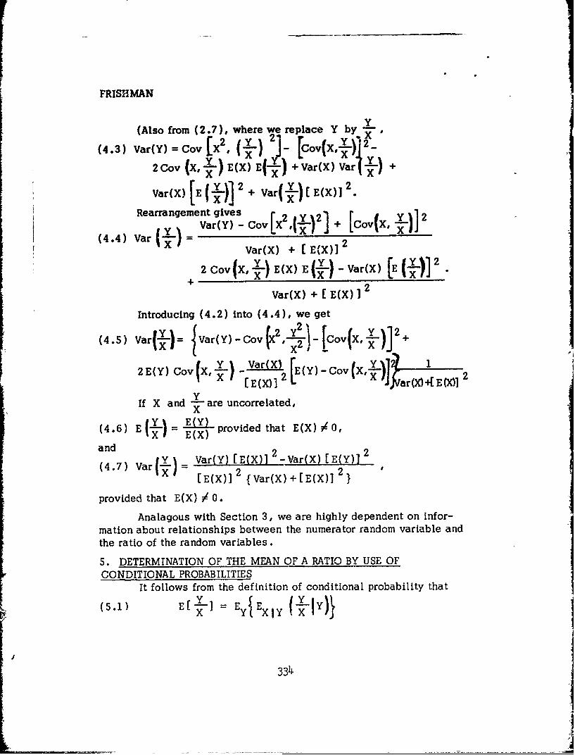
(Also from (2.7), where we replace Y by "

Rearrangement ygives CorI2 , 1Y-)]+[o(,x--(4.4) Var Var(Y) Cv (-) J [-

Var(X) + [E(X)1 2

2 Co(X, ) E(X) E -) -VarX [E -)]2

+

V - Var(X) + [ E(X) ] 2

Introducing (4.2) into (4.4), we get

Va(Y -ovox(4.5) Var (-) = -

Vat(X) + 1

2 Cov(X) VrE(X) IE(Y)- CoV"(X ar(X E0X[E (X) + E2(X

If X ad areuncorrelated,(4I6)Eo E(X) providedthat E(X) ,and 2 2

(4.7) Var-Y) = Var(Y) [E(X) -Var(X) [E(y) 2

VaX 21 2

[E(X)] {Var(X) +[E(X)] 2

provided that E(X) 0.

Analagous with Section 3, we are highly dependent on infor-mation about relationships between the numerator random variable andthe ratio of the random variables.

5. DETERMINATION OF THE MEAN OF A RATIO BY USE OFCONDITIONAL PROBABILITIES

It follows from the definition of conditional probability that

(5.1) E[- -= {jEXY (Ey-EIYx

334 I

FRISHMAN

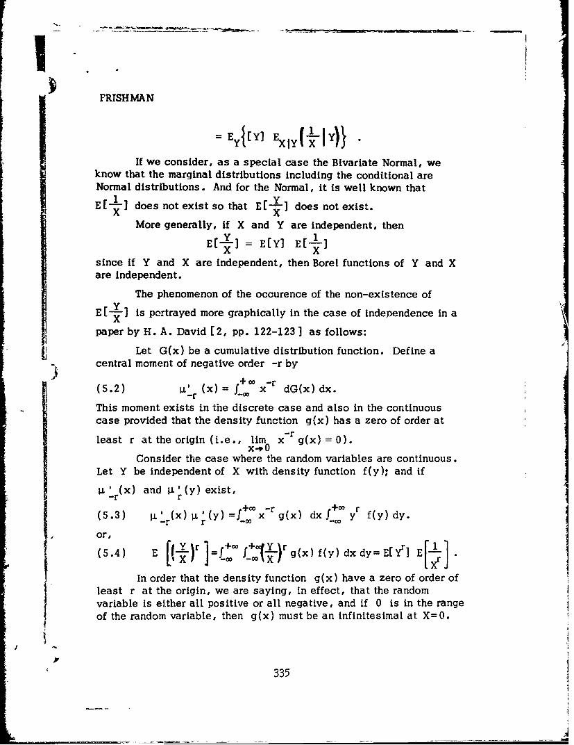
-EyjEY1 EXtY(ttY)

If we consider, as a special case the Bivariate Normal, weknow that the marginal distributions including the conditional areNormal distributions. And for the Normal, it is well known that

x]-L does not exist so that E[Y does not exist.1 Y

More generally, if X and Y are independent, then

since if Y and X are independent, then Borel functions of Y and Xare independent.

The phenomenon of the occurence of the non-existence of

x[-] is portrayed more graphically in the case of independence in aE

paper by H. A. David [2, pp. 122-123 1 as follows:

Let G(x) be a cumulative distribution function. Define acentral moment of negative order -r by

(5.2) t (x)= f0 x - r dG(x) dx.

This moment exists in the discrete case and also in the continuouscase provided that the density function g(x) has a zero of order at

least r at the origin (i.e., lim x- r g(x) = 0).x-*0

Consider the case where the random variables are continuous.Let Y be independent of X with density function f(y); and if

L I W(x) and P.' (y) exist,-r r+oo -r +00 r

(5.3) W._r(X).(Y) = .x g(x) dx fL y f(y) dy.

or,

(5.4) E FiXr r00 XIYr )f(y) dxdy =E[ Yrl Er1In order that the density function g(x) have a zero of order of

least r at the origin, we are saying, in effect, that the randomvariable is either all positive or all negative, and If 0 is in the rangeof the random variable, then g(x) must be an infinitesimal at X=0.

335

FRISHMAN

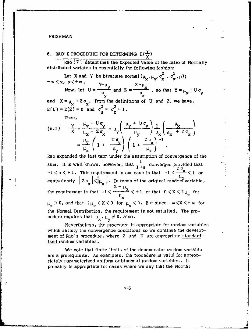
6. RAO' S PROCEDURE FOR DETERMING E(K)

Rao [ 7 ] determines the Expected Value of the ratio of Normallydistributed variates in essentially the following fashion:

Let X and Y be bivariate normal (ix, , a2 , a ,p);- oo<x, y<+o. x yY- an Z - x - x

Now, let U- and Z a , sothat Y=y +Ua y

and X = Px + Z a . From the definitions of U and Z, we have,E(U)=E(Z)=0 and a 2

u zThen,

(6.1) X Lx + Z (Y -y ) yx a

xxI I + ___ 1 + .

Rao expanded the last term under the assumption of convergence of the

sum. It is well known, however, that converges provided that1+a Za

-1 <a <+ 1. This requirement in our case is that -1 <-a- < 1 or

equivalently ZaI < I j. In terms of the original random variable,1X-

P xthe requirement is that -1< <+1 or that 0< X<2 x forxp > 0, andthat 2 1x<X<0 for p <0. Butsince -oo<X<+oo for

the Normal Distribution, the requirement is not satisfied. The pro-cedure requires that V x, p y ? 0, also.

Nevertheless, the procedure is appropriate for random variableswhich satisfy the convergence conditions so we continue the develop-ment of Rao' s procedure, where Z and U are appropriate standard-ized random variables.

We note that finite limits of the denominator random variableare a prerequisite. As examples, the procedure is valid for approp-riately parameterized uniform or binomial random variables. Itprobably is appropriate for cases where we say that the Normal

336

?i

• 1....

FRISHMAN

distribution satisfies the data, since we probably nean that a trun-cated Normal satisfies the data, it being rare for an item or testmeasurement to take on both positive and negative values. By slightlyrewriting (6.1) and performing the expansion we obtain

(6.2) U x + Z2 . 3

+ + .

= 22 3X X PX

Cr V U 2 Ua2

+ Y x U +x ...x x

Taking Expected Values, we obtain

PV - + 2E(Z2) a E(Z3)(6.3) E- + Il xLX 2 3

(-l)' ar E(Z) )rIaE(U+ x } {

M

a2 E Z2 U_,n-1ian E nU

2 +n*~

00 (- )Z

I1 i=2 If /3

+ a E xY J=1 j +1

If, in addition to the prior conditions on the range of X andtha t p. ? 0, we specify that Z, U are bivariate central symmetrically

rdistributed. Then from [8, pp. 23], we have that

-' 337

FRISHMAN

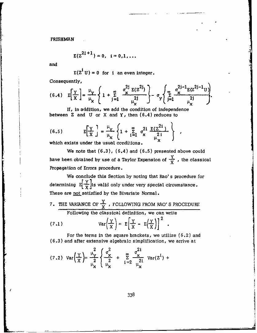
E(Z 2 1 + 1 )=O, i=0,1,...

and

E(Z i U) =0 for i an even integer.

Consequently,

(6.4) E- 3 1 + Z (-- 2j 2 Txx x

If, in addition, we add the condition of independencebetween Z and U or X and Y, then (6.4) reduces to

rY = -Y ~ 21 E(Z 21(6.5) E [ = x + x a

x f x

which exists under the usual conditions.

We note that (6.3), (6.4) and (6.5) presented above could

have been obtained by use of a Taylor Expansion of -L , the classicalxPropagation of Errors procedure.

We conclude this Section by noting that Rao' s procedure for

determining E[-LJis valid only under very special circumstance.

These are not satisfied by the Bivariate Normal.

Y7. THE VARIANCE OF - , FOLLOWING FROM RAO' S PROCEDURE

Following the classical definition, we can write

(7.1) Va r (7 E [Y- E .Y)

For the terms in the square brackets, we utilize (6.2) and

(6.3) and after extensive algebraic simplification, we arrive at

2 a 2 21

(7.2) Var = . -- + 2Var(Z

lx ~x i=2 3 x

3348

FRISHMAN

i +k

2 X X ~I- (I Cov(Zi Zi=k k-2 k

I<k

+ 2~ (--- Cov(ZU) +2x 1+x

a i+ j

E 1 (-1)'+J x ,zJx-- J= 1 1± J

v ; + : Var(Z~uJ2 j 12jx Ilk

COj +m+ 2 (-E Cov(Z IT. zmU)

j=O m=1 j +mJ<m ' X

) where, for example, Var (Zj U) = E [ Zj U-E (Z U)] 2

Cov (Z1 U, zmu )= E[ZJ U-E (Zj U)] zmU-E (Zmu)

Cov(Z,U)=E[Z-E(Z)l [U-E(U)] =E(ZU).

If we take only the first term in each of the curly brackets, weobtain an approximation 2

p2 a2 P p a(7.3) Var(-' ' " 2 , + +

x -2xL) 4 -3 2Lx Lx 11x

22 22!za + JLa- 2ppa

4

which can be obtained, also, by the usual Propogation of Errorsprocedures.

If we specify that X and Y (and consequently U and Z) areindependent, then (7.2) reduces to

S339

FRISHMAN

2 2 21

(7.4) Vax= - + Var(Z i ) +2 2 i 2 2

x Px Ixi+k2)

2a E x (1)i+k Cvzi ki=1 k=2 i+k Cov(ZiZi<k 'xa2 2J Va 7a 2 0'2

2 1 + = 2j

Ix P xand the approximation reduces to

22 22

(7.5) Var ) x 4 y

8. THE DISTRIBUTION OF THE RATIO OF NORMAL VARIATESC. C. Craig [ 1, pp. 24-32 1 presents Fieller' s development

[3, pp. 424-440 1 on the distribution of a ratio and Geary' s approxi-mation [4, pp. 442-460 1 . The following is a summary of the results:

2 2Thn Assum (x,Y) is Bivarae Normal or BVN (Ix, ,, ,ia p).

(8.1) f(x,y) 27T(1-l2)1/2 e-1/2(1-p2I-x )2

+ x

' Let V= - - a n d let x =x. Then, dvdax-

(8.2) g(v)=f +Ixtf(x,xv) dx = f0 x f(x,xv) dx - fox f(x,xv)dx

+00 0

Q xv =xf ddxdyandeRde)in

Len x f(x,xv)dx-2 fo x f(x,xv) dxLetting

Q(v) =.Cox f(x,xv) dx, and R(v) f0-2x f(x,xv) dx, then

34o

iI

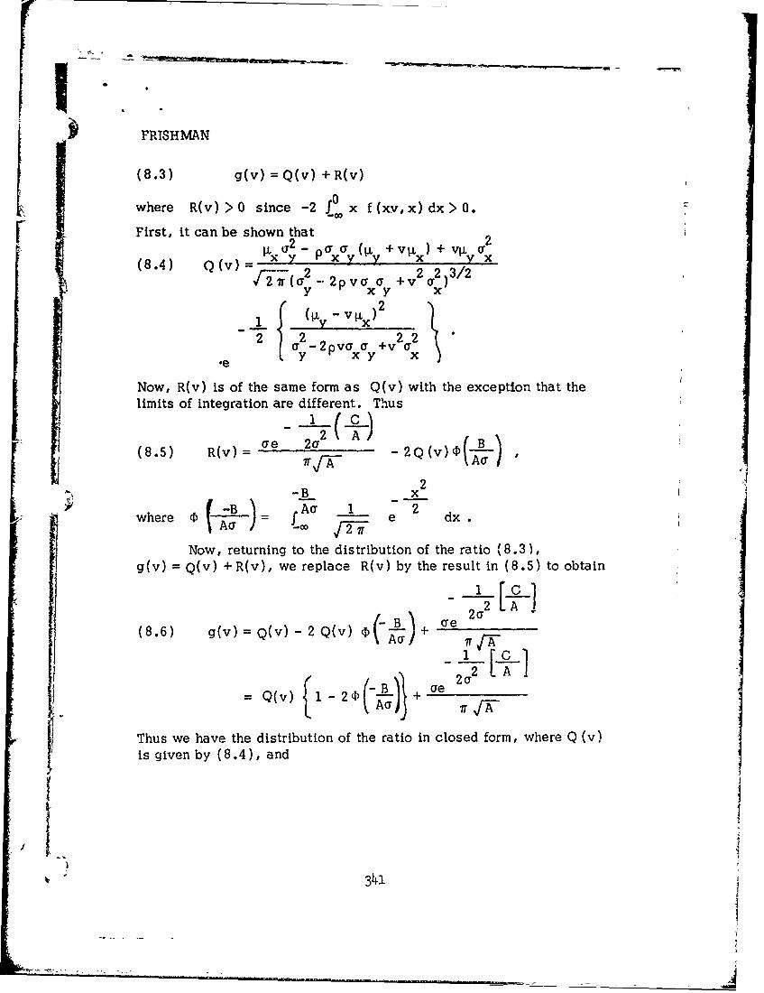
(8.3) g(v) =Q(v) +R(v)

where R(v) >0 since -2 t0 x f(xv, x) dx>0.First, it can be shown that 2t U2 - ( Y + v x ) V L x(8.4) Q(v)=Ir 2. 2pva a +,2 2)3/2

2 {a 2 2pvY a +V 2a 2

xy x

Now, R(v) is of the same form as Q(v) with the exception that thelimits of integration are different. Thus

(8.5) R(v) = ae 2-2Q(v) -

-x 2

f-B\ fAU 1 2where 1 - - e dx.

Now, returning to the distribution of the ratio (8.3),g(v) = Q(v) +R(v), we replace R(v) by the result in (8.5) to obtain

2a2

(8.6) g(v)=Q(v)-2Q(v) )(-B)+ ae

= Q(v) 1-2(

Thus we have the distribution of the ratio in closed form, where Q (v)is given by (8.4), and

" 341IqmI

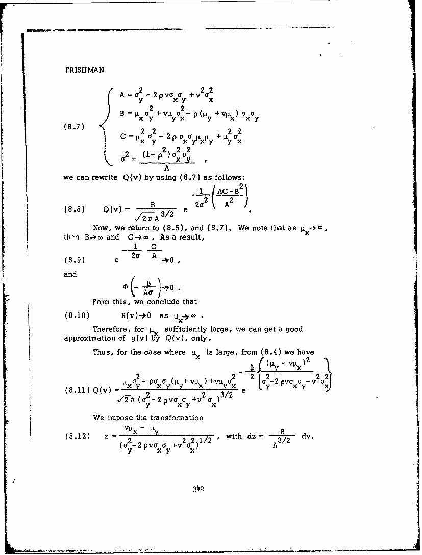
FRISHMAN

A: -2pvra +v ay x y x

B=i 2+ a2 ( +v )aa

(8.7) 2 2 2 2C=Zx2-° 0.y x y x y + Yo

S2= ( 1_ 02) a2 a2

we can rewrite Q(v) by using (8.7) as follows:

(8.8) Q(v) = B (c -2A/2)

Now, we return to (8.5), and (8.7). We note that as x-c,t--n B-* c and C- oo . As a result,

1 C2--U A(8.9) e . 0,

and ,( B-AaJ

From this, we conclude that

(8.10) R(v)-*0 as ix-)co

Therefore, for L sufficiently large, we can get a goodapproximation of g(v) by Q(v), only.

Thus, for the case where [jx is large, from (8.4) we have

2 2 2 2 2 2xy xy xyy x xy

(8.,11 Q((v) e22 +v 2 )3/2

y y x

We impose the transformationV[Lx- Ly

_ B(8.12) z 2 v a 21/2 with dz- 3/2 dv,

(a y - 2 P v X y x+v a A

342

- .',.-,

~FRISHMAN

and we note that the denominator of Q(v) is positive for all v.Hence ." Val - u.. ]

(8.13) Q(z)= Q 2 V 2 2)1/2

x yIt follows that, as Lx-L'* for afinite, z approaches a N(0,11.

This is the Geary result[4 1 . x

If in (8.6), ux = ty = 0, we obtain

p..2)1/2

(8.14) g 1 (v). (1- P2 1 a

r Y xIT( ~- 2 Pv +v 2 -

a generalized Cauchy distribution.

The cumulative distribution function for (8.14) is

1 1-p(8.151 G(v)= fV~gv dv ar tg .arx vPa y ]

as obtained from Gradstein and Ryzhik, [ 6, p. 82].

The generalized Cauchy obtained by this writer is a simpleextension and has utility more from a theoretical viewpoint than anapplications viewpoint.

However, the Geary result has great applicability as do theapproximation results in Sections 6 and 7 when one is willing toassume that X and Y are Bivariate Normal. As noted in Section 6,in the real world, few if any, random variables are truly normallydistributed since few, if any, can range from - oo to + oo. Few, if any,

will take on both positive and negative values! Thus the mathematical

abstraction, the Normal Distribution, can be at best a good approxi-mation, and a good approximation only around the mean of the data,since ordinarily one does not see data points in the extreme tails ofthe Distribution.

34 3

FRISHMAN

9. SUMMARY

In Sections 3 and 4, exact expressions are given for the Meanand the Variance of a Ratio of random variables, regardless of the formof the random variables. One problem is that certain correlation co-efficients must be known or assumed to be zero in order to use theformulae. Also, there is the usual requirement that the moments exist.Based on the results of Section 5, we know that these exact resultsare not appropriate for the Normal Distribution and those other distri-butions where the random variable takes on negative and positivevalues and/or the value 0 with probability greater than 0.

In Section 6, a procedure is given for getting the Mean of aRatio. The requirement is that the denominator random variable besuch that either 2ix<X <0 when px Is negative or that 0<X<2 xwhen p is positive. Also, we require that the Mean of the numerator

10. In Section 7, we obtain the Variance. Since the results inboth Sections require summing infinite series, approximations can beobtained by terminating the summation wherever desired.

Finally in Section 8, we sketch out the development for anapproximation of the distribution of the ratio if both random variablesare Normally Distributed, in the sense that the Denominator variabledoes not take on both positive and negative values. It is claimed thatit is rare for actual random variables to be Normally distributed in themathematical sense. Rather, the Normal Distribution is a reasonableapproximation at best, and under these circumstances, the resultspresented in Sections 6,7 and 8 are appropriate to be used.

10. BIBLIOGRAPHY

1. Craig, C. C. (1942) "On Frequency Distributions of the Quotientand of the Product of Two Statistical Variables", Amer. Math.Monthly, Vol. 49, No. 1.

2. David, H. A. (1955) "Moments of Negative Order and Ratio-Statistics", Journal of the Royal Stat. Society, Part 1.

3. Fieller, E. C. (1932) "The Distribution of the Index in a NormalBivariate Population", Biometrika, Vol. 24.

4. Geary, R. C. (1932) "The Frequency Distribution of the Quotientof two Normal Variables", Journal of the Royal StatisticalSociety, Vol. 93.

3341ij.

-

FRISHMAN

S. Goodman, L. (1960) "On the Exact Variance of Products",Journal of the American Stat. Assn., Vol. 55.

6. Gradstein, I. S. and Ryzhik, I. M. (1965) Tables of Integrals,Series and Products. Academic Press.

7. Rao, C. R. (1952) Advanced Statistical Methods in Biometrics

Research. John Wiley and Sons, Inc.8. Frishman, F. (1971) "On Ratios of Random Variables and an

Application to a Non-linear Regression Problem". Ph.D.dissertation, The George Washington University.

34

I 345

I