Embed Size (px)
Citation preview
Energies 2014, 7, 6620-6644; doi:10.3390/en7106620
energies ISSN 1996-1073
www.mdpi.com/journal/energies
Article
Real-Time Wavelet-Based Coordinated Control of
Hybrid Energy Storage Systems for Denoising and
Flattening Wind Power Output
Tran Thai Trung 1, Seon-Ju Ahn 1,*, Joon-Ho Choi 1, Seok-Il Go 1 and Soon-Ryul Nam 2
1 Department of Electrical Engineering, Chonnam National University, Gwangju 500-757, Korea;
E-Mails: [email protected] (T.T.T.); [email protected] (J.-H.C.);
[email protected] (S.-I.G.) 2 Department of Electrical Engineering, Myongji University, Yongin 449-728, Korea;
E-Mail: [email protected]
* Author to whom correspondence should be addressed; E-Mail: [email protected];
Tel.: +82-62-530-1738; Fax: +82-62-530-1749.
External Editor: Frede Blaabjerg
Received: 30 July 2014; in revised form: 25 September 2014 / Accepted: 9 October 2014 /
Published: 16 October 2014
Abstract: Since the penetration level of wind energy is continuously increasing, the negative
impact caused by the fluctuation of wind power output needs to be carefully managed.
This paper proposes a novel real-time coordinated control algorithm based on a wavelet
transform to mitigate both short-term and long-term fluctuations by using a hybrid
energy storage system (HESS). The short-term fluctuation is eliminated by using an
electric double-layer capacitor (EDLC), while the wind-HESS system output is kept
constant during each 10-min period by a Ni-MH battery (NB). State-of-charge (SOC)
control strategies for both EDLC and NB are proposed to maintain the SOC level of
storage within safe operating limits. A ramp rate limitation (RRL) requirement is also
considered in the proposed algorithm. The effectiveness of the proposed algorithm has
been tested by using real time simulation. The simulation model of the wind-HESS system
is developed in the real-time digital simulator (RTDS)/RSCAD environment. The proposed
algorithm is also implemented as a user defined model of the RSCAD. The simulation
results demonstrate that the HESS with the proposed control algorithm can indeed assist in
dealing with the variation of wind power generation. Moreover, the proposed method
OPEN ACCESS
Energies 2014, 7 6621
shows better performance in smoothing out the fluctuation and managing the SOC of
battery and EDLC than the simple moving average (SMA) based method.
Keywords: wind generation; electrical energy storage system (EESS); real-time wavelet
transform; energy management; fluctuation mitigation; real time digital simulation;
Ni-MH battery (NB); electric double-layer capacitor (EDLC)
1. Introduction
Recently, the exhaustion of fossil fuels and the critical environmental pollution have led to the need
to develop new clean energy sources. Wind energy, a type of renewable and environmental-friendly
energy, is considered as a prospective replacement for conventional energy resources. However,
because of the stochastic and intermittent characteristic of wind speed, the resulting fluctuation in power
output is the greatest obstacle to the increasing penetration level of wind power in power grids [1].
In order to reduce the negative impact of these fluctuations on the stability, reliability and protection of
the power system, a number of control methods have been proposed.
Many researchers have demonstrated that pitch angle control, in conjunction with other modern
controllers such as the fuzzy logic controller, provides a very effective means of regulating
aerodynamics to reduce wind power fluctuation [2]. However, the short-term fluctuations of wind
power output cannot be mitigated by these types of controllers because of the mechanical stress
accrued by the wind blade. Abedini et al. [3] used a rotor inertia adjustment method to smooth out
wind power output. This approach also does not require any energy storage devices but the rotor speed
no longer can be controlled to follow maximum power tracking.
An electrical energy storage system (EESS) is recognized as an alternative technique to mitigate
both short-term and long-term wind power fluctuations. Various benefits of using EESS in wind
power applications are discussed in [4]. The cooperation of different storage devices with different
charge/discharge characteristics makes it possible to balance both power- and energy-scale requirements.
Among various hybrid energy storage system (HESS) options, this paper focuses on the Ni-MH
battery (NB)-electric double-layer capacitor (EDLC) HESS as a solution to mitigate the wind
power fluctuation. EDLC is suitable for denoising wind power output because it has a number of
exceptional characteristics, including high power density, fast charge/discharge process, high efficiency,
and long lifetime [5]. On the other hand, NB with high energy density characteristic is fit for flattening
wind power fluctuations.
In the existing literature, a moving average technique and the first-order delay filter (FDF), the
simplest methods, have been applied to smooth out wind power fluctuation [6–10]. Ushiwata et al. [6]
presented a smoothing approach to mitigate wind power fluctuations using EDLC and the simple
moving average (SMA) control method. Tanabe et al. [7] used FDF with an adjustable time constant
and additional rate limiter to keep the fluctuation of wind power output within 10% for 20 min,
while Sheikh et al. [8] proposed a hybrid control algorithm including both SMA and exponential
moving average (EMA) to generate output power reference of static synchronous compensator
(STATCOM)/superconducting magnetic energy storage (SMES) system. A state-of-charge (SOC)
Energies 2014, 7 6622
regulation method of a battery in a hybrid wind power/battery energy storage system has been
proposed in [9], and hardware-in-the-loop (HIL) simulation studies of a wind turbine coupled with
battery supercapacitor EESS has been presented in [10]. Both are based on simple filtering algorithms.
Some researchers have proposed intelligent approaches for EESS power dispatching and scheduling.
Suvire et al. [11] utilized a fuzzy inference system to control the active power of the distribution static
synchronous compensator (DSTATCOM) coupled with flywheel energy storage system to smooth out
wind power fluctuation, whereas Mishra et al. [12] used a bacteria foraging technique to integrate
wind turbine and batteries to maintain a constant grid power output. Li et al. [13] proposed a control
algorithm cooperating wavelet transform with fuzzy logic control to smooth a hybrid system including
photovoltaic and wind power systems by using a battery energy storage system. However, these methods
are implemented via non-real time process, which limits the real-time application. Furthermore, they failed
to neither ensure the system power output always satisfies ramp rate requirements nor consider to safe
working limits of EESS. Jiang et al. [14] implemented a wavelet-based capacity configuration and
coordinated control algorithm for reducing output power fluctuations of a wind system using a
lithium-ion battery-ultra-capacitor energy storage system. Although this paper proposed a novel
approach for solving most of the above problems, it still used two stages of wavelet filtering that
increase the computational complexity and require wind data prediction algorithm. The various
features of the previous researches are summarized in Table 1.
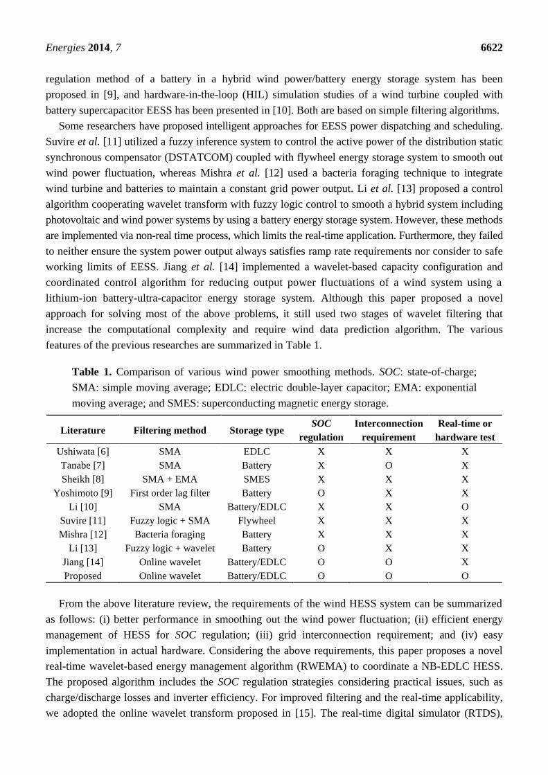
Table 1. Comparison of various wind power smoothing methods. SOC: state-of-charge;
SMA: simple moving average; EDLC: electric double-layer capacitor; EMA: exponential
moving average; and SMES: superconducting magnetic energy storage.
Literature Filtering method Storage type SOC
regulation
Interconnection
requirement
Real-time or
hardware test
Ushiwata [6] SMA EDLC X X X
Tanabe [7] SMA Battery X O X
Sheikh [8] SMA + EMA SMES X X X
Yoshimoto [9] First order lag filter Battery O X X
Li [10] SMA Battery/EDLC X X O
Suvire [11] Fuzzy logic + SMA Flywheel X X X
Mishra [12] Bacteria foraging Battery X X X
Li [13] Fuzzy logic + wavelet Battery O X X
Jiang [14] Online wavelet Battery/EDLC O O X
Proposed Online wavelet Battery/EDLC O O O
From the above literature review, the requirements of the wind HESS system can be summarized
as follows: (i) better performance in smoothing out the wind power fluctuation; (ii) efficient energy
management of HESS for SOC regulation; (iii) grid interconnection requirement; and (iv) easy
implementation in actual hardware. Considering the above requirements, this paper proposes a novel
real-time wavelet-based energy management algorithm (RWEMA) to coordinate a NB-EDLC HESS.
The proposed algorithm includes the SOC regulation strategies considering practical issues, such as
charge/discharge losses and inverter efficiency. For improved filtering and the real-time applicability,
we adopted the online wavelet transform proposed in [15]. The real-time digital simulator (RTDS),
Energies 2014, 7 6623
which provides reliable and accurate computation in hard real time, is used to model the system and to
implement and validate the proposed algorithm [16].
This paper is organized as follows: Section 2 presents the modeling of each energy storage device;
Section 3 introduces the RWEMA; in Section 4, the simulation studies are carried out in the
RTDS/RSCAD environment to validate the effectiveness of the proposed algorithm; finally, some
conclusions are given in Section 5.
2. Wind-Hybrid Energy Storage System Modeling in RSCAD
Integrating EESS with a wind power system will reduce the power output fluctuation. In order to
reduce both short-term and long-term fluctuations, this paper proposes the combination of the NB and
EDLC energy storage system to satisfy both high power and energy capacity requirements.
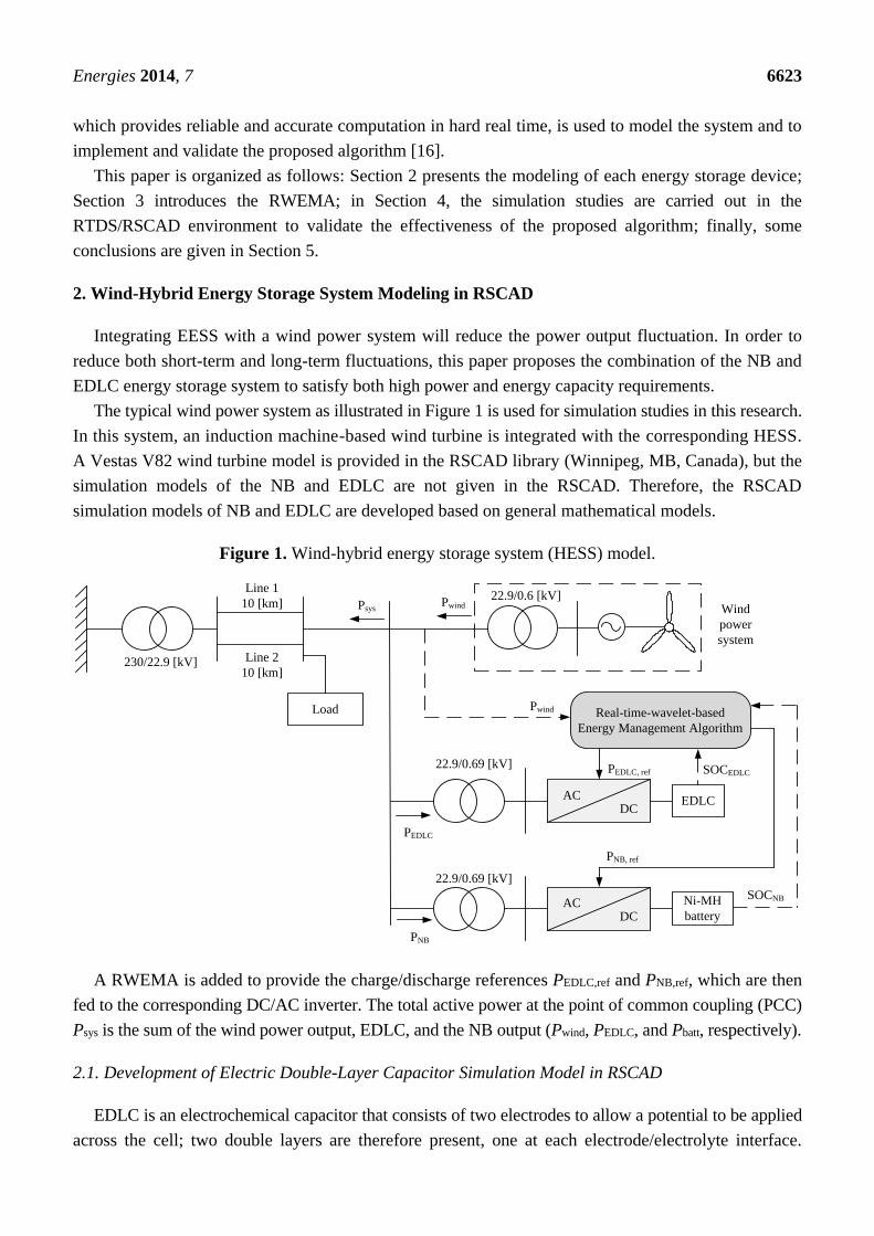
The typical wind power system as illustrated in Figure 1 is used for simulation studies in this research.
In this system, an induction machine-based wind turbine is integrated with the corresponding HESS.
A Vestas V82 wind turbine model is provided in the RSCAD library (Winnipeg, MB, Canada), but the
simulation models of the NB and EDLC are not given in the RSCAD. Therefore, the RSCAD
simulation models of NB and EDLC are developed based on general mathematical models.
Figure 1. Wind-hybrid energy storage system (HESS) model.
A RWEMA is added to provide the charge/discharge references PEDLC,ref and PNB,ref, which are then
fed to the corresponding DC/AC inverter. The total active power at the point of common coupling (PCC)
Psys is the sum of the wind power output, EDLC, and the NB output (Pwind, PEDLC, and Pbatt, respectively).
2.1. Development of Electric Double-Layer Capacitor Simulation Model in RSCAD
EDLC is an electrochemical capacitor that consists of two electrodes to allow a potential to be applied
across the cell; two double layers are therefore present, one at each electrode/electrolyte interface.
Load
ACDC
EDLC
ACDC
Ni-MH
battery
Real-time-wavelet-based
Energy Management Algorithm
Wind
power
system
SOCNB
SOCEDLCPEDLC, ref
PNB, ref
230/22.9 [kV]
22.9/0.69 [kV]
22.9/0.69 [kV]
22.9/0.6 [kV]
Pwind
Line 1
10 [km]
Line 2
10 [km]
Psys
PEDLC
PNB
Pwind
Energies 2014, 7 6624
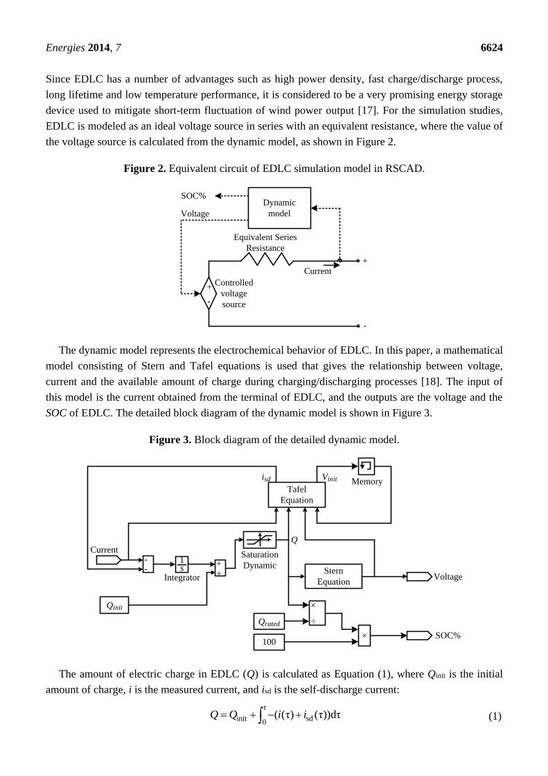
Since EDLC has a number of advantages such as high power density, fast charge/discharge process,
long lifetime and low temperature performance, it is considered to be a very promising energy storage
device used to mitigate short-term fluctuation of wind power output [17]. For the simulation studies,
EDLC is modeled as an ideal voltage source in series with an equivalent resistance, where the value of
the voltage source is calculated from the dynamic model, as shown in Figure 2.
Figure 2. Equivalent circuit of EDLC simulation model in RSCAD.
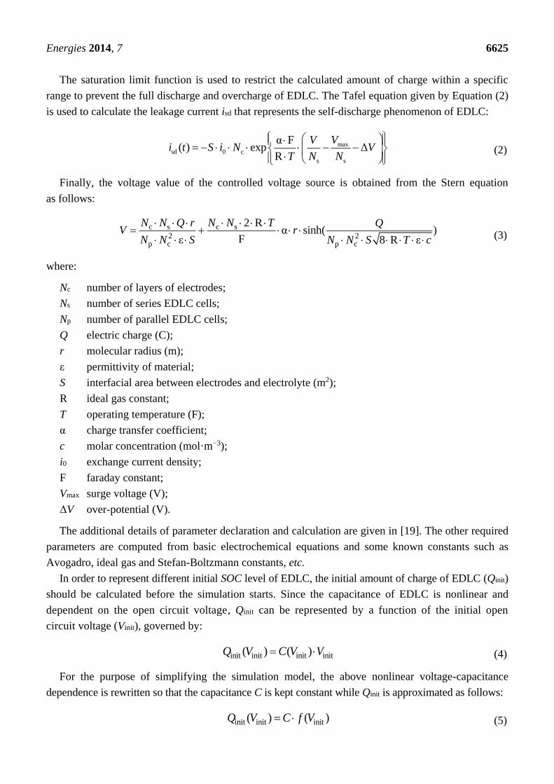
The dynamic model represents the electrochemical behavior of EDLC. In this paper, a mathematical
model consisting of Stern and Tafel equations is used that gives the relationship between voltage,
current and the available amount of charge during charging/discharging processes [18]. The input of
this model is the current obtained from the terminal of EDLC, and the outputs are the voltage and the
SOC of EDLC. The detailed block diagram of the dynamic model is shown in Figure 3.
Figure 3. Block diagram of the detailed dynamic model.
The amount of electric charge in EDLC (Q) is calculated as Equation (1), where Qinit is the initial
amount of charge, i is the measured current, and isd is the self-discharge current:
init sd0( (τ) (τ))dτ
tQ Q i i (1)
+
Voltage
Equivalent Series
Resistance
Current
-
+
-
Dynamic
model
SOC%
Controlled
voltage
source
Tafel
Equation
Memory
1s
Qinit
Stern
Equation
Qrated
100
×
÷
--
×
isd Vinit
Integrator
Saturation
Dynamic
Current
Voltage
SOC%
++
Q
Energies 2014, 7 6625
The saturation limit function is used to restrict the calculated amount of charge within a specific
range to prevent the full discharge and overcharge of EDLC. The Tafel equation given by Equation (2)
is used to calculate the leakage current isd that represents the self-discharge phenomenon of EDLC:
maxsd 0 c
s s
α F( ) exp Δ
R
VVi t S i N V
T N N
(2)
Finally, the voltage value of the controlled voltage source is obtained from the Stern equation
as follows:
c s c s
2 2p c p c
2 Rα sinh( )
Fε 8 R ε
N N Q r N N T QV r
N N S N N S T c
(3)
where:
Nc number of layers of electrodes;
Ns number of series EDLC cells;
Np number of parallel EDLC cells;
Q electric charge (C);
r molecular radius (m);
ε permittivity of material;
S interfacial area between electrodes and electrolyte (m2);
R ideal gas constant;
T operating temperature (F);
α charge transfer coefficient;
c molar concentration (mol·m−3);
i0 exchange current density;
F faraday constant;
Vmax surge voltage (V);
ΔV over-potential (V).
The additional details of parameter declaration and calculation are given in [19]. The other required
parameters are computed from basic electrochemical equations and some known constants such as
Avogadro, ideal gas and Stefan-Boltzmann constants, etc.
In order to represent different initial SOC level of EDLC, the initial amount of charge of EDLC (Qinit)
should be calculated before the simulation starts. Since the capacitance of EDLC is nonlinear and
dependent on the open circuit voltage, Qinit can be represented by a function of the initial open
circuit voltage (Vinit), governed by:
init init init init( ) ( )Q V C V V (4)
For the purpose of simplifying the simulation model, the above nonlinear voltage-capacitance
dependence is rewritten so that the capacitance C is kept constant while Qinit is approximated as follows:
init init init( ) ( )Q V C f V (5)

Energies 2014, 7 6626
The function f(Vinit) is obtained for a specific EDLC module under test, which consists of 3000 F
Maxwell BootsCap Devices (San Diego, CA, USA). For this, the simulation is implemented with an
EDLC model provided by Simscape module in MATLAB Simulink [19]. The Qinit data is captured by
changing the initial voltage from 0 V to 2.8 V (equivalent to SOC level from 0% to 100%) while the
EDLC is either fully charged or fully discharged with a constant current. From the simulation data,
the relationship between Vinit and Qinit is established by curved fitting as follows:
6 5 4 3init init init init init
2init init
( ) 0.001822 ( ) 0.018478 ( ) 0.073154 ( ) 0.125816 ( )
0.012911 ( ) 0.766703 ( ) 0.001655
f V V V V V
V V
(6)
Based on the above mathematic model, a user-defined model (UDM) of EDLC is made by using
the component builder in the RSCAD. From the configuration interface of the developed UDM,
the parameters of EDLC can be modified to satisfy the requirements of different simulation cases,
as shown in Figure 4.
Figure 4. EDLC model parameter configuration menu.
2.2. Development of Ni-MH Battery Simulation Model in RSCAD
The first NB was introduced in 1990 by Sanyo Electric Company in Osaka, Japan. This battery type
has a number of advantages such as having high energy density and high efficiency, and containing no
toxic metals. Since its response is slower than EDLC, it is used to reduce long-term wind
power fluctuation.
NB is also modeled as a controllable voltage source, where the value of the voltage source is
calculated from the dynamic model. In this study, the modified Shepherd-based mathematic model of
NB presented in [20] is used. This model includes an equation to describe the electrochemical behavior
of a battery directly in terms of terminal voltage, open circuit voltage, internal resistance, discharge current,
and SOC. This model is based on a number of specific assumptions and limitations, including the
internal resistance is supposed to be constant and temperature effect is not considered.
Energies 2014, 7 6627
The value of the voltage source during the discharge and charge process can be calculated by using
Equations (7) and (8), respectively:
*batt 0 b ( ) Exp( )
QV E R i K it i t
Q it
(7)
*batt 0 b
Pol. Voltage
Exp( )0.1
Q QV E R i K i K it t
it Q Q it
(8)
where:
Vbatt battery voltage (V);
E0 battery constant voltage (V);
K polarization constant (V/A·h) or polarization resistance (Ω);
Q battery capacity (A·h);
it actual battery charge (A·h);
A exponential zone amplitude (V);
B exponential zone time constant inverse (A·h)−1;
R internal resistance (Ω);
i battery current (A);
i* filtered current (A).
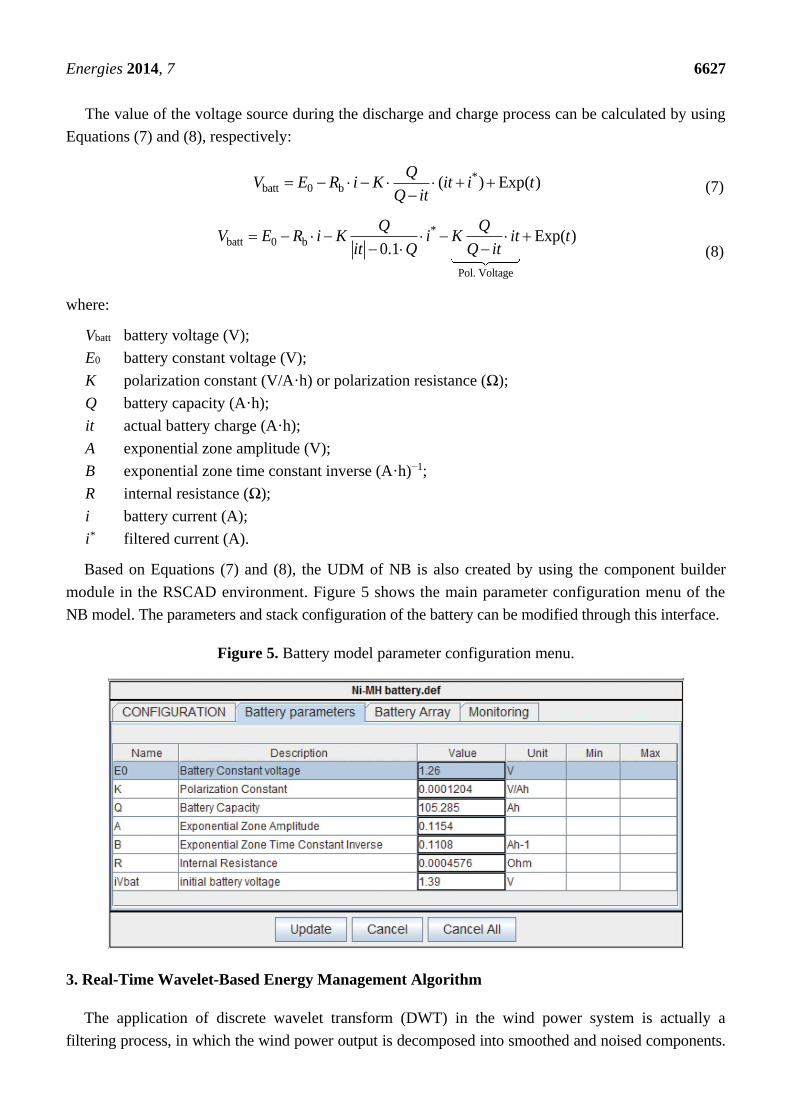
Based on Equations (7) and (8), the UDM of NB is also created by using the component builder
module in the RSCAD environment. Figure 5 shows the main parameter configuration menu of the
NB model. The parameters and stack configuration of the battery can be modified through this interface.
Figure 5. Battery model parameter configuration menu.
3. Real-Time Wavelet-Based Energy Management Algorithm
The application of discrete wavelet transform (DWT) in the wind power system is actually a
filtering process, in which the wind power output is decomposed into smoothed and noised components.
Energies 2014, 7 6628
This process can be classified into non-real-time and real-time methods. In this paper, a real-time
wavelet method is implemented based on a moving window function (MWF) [15]. This MWF has a
length of n and is designed to store wind power output data as a first-in first-out buffer. The proposed
RWEMA controller dynamically obtains the results from MWF and the SOC from the EDLC and
NB bank, and then determines the reference value for the corresponding DC/AC inverter controller
of HESS. Furthermore, the SOC control strategies are added to maintain the SOC levels of storage
within their safe operating limits, which are normally between 20% and 80% for battery [14] and
between 30% and 90% for EDLC.
The objective of the proposed RWEMA is to both denoise and flatten the total wind-HESS system
output during the specified time period. In order to obtain a constant total power output every 10 min,
an average buffer with a length of m is used in the RWEMA. The procedure of the proposed
RWEMA consists of three key stages: data processing and DWT procedure, SOC control strategy,
and ramp rate limitation (RRL).
3.1. Data Processing and Discrete Wavelet Transform Procedure
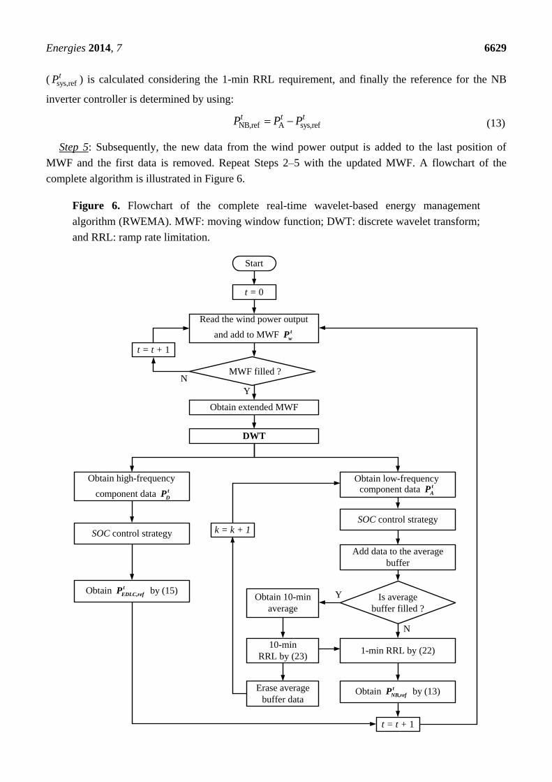
Step 1: During the first n seconds, the wind power output data is sampled every second and added to
the MWF:
1, 2, ..., 1, twP t n n (9)
Step 2: As soon as the MWF is filled, the MWF is extended by using a short-symmetric method to
deal with some of the disadvantages of real-time wavelet transform such as border distortion and the
pseudo-Gibbs phenomena [15]. The length of MWF is increased, and the pre-processed wind power
series becomes:
1 2 1 1 Δ
Short-Symmetric
, ,..., , , , ,...,n n n n n tw w w w w w wP P P P P P P
(10)
Step 3: The wind power output in the extended MWF is decomposed into two corresponding
components by passing it through low-pass and high-pass filter to the l-th level. The level-l low-frequency
component and the sum of the l-level high-frequency terms are:
1, 2,..., 1, , , 1,..., ΔtAP t n n n n n t
(11)
1, 2,..., 1, , , 1,..., ΔtDP t n n n n n t
(12)
Step 4: The n-th data of the high and low frequency component are sent to SOC control strategy
stage described in Section 3.2. The modified high frequency component is directly used to determine
the active power reference for the inverter controller of EDLC. The modified low frequency
component is then added to the average buffer. As soon as the average buffer is filled, the system
output reference for the next 10 min ( sys,refkP ) is calculated by taking the average of the buffer and
applying the 10-min RRL constraint given in Section 3.3. The system output reference at time t
Energies 2014, 7 6629
( sys,reftP ) is calculated considering the 1-min RRL requirement, and finally the reference for the NB
inverter controller is determined by using:
NB,ref A sys,reft t tP P P (13)
Step 5: Subsequently, the new data from the wind power output is added to the last position of
MWF and the first data is removed. Repeat Steps 2–5 with the updated MWF. A flowchart of the
complete algorithm is illustrated in Figure 6.
Figure 6. Flowchart of the complete real-time wavelet-based energy management
algorithm (RWEMA). MWF: moving window function; DWT: discrete wavelet transform;
and RRL: ramp rate limitation.
Start
t = 0
Obtain extended MWF
DWT
t = t + 1
Obtain 10-min
average
SOC control strategy
Obtain low-frequency component data t
AP
Obtain high-frequency
component data t
DP
Obtain by (15)t
EDLC,refP
N
Y
N
Y
t = t + 1
Read the wind power output
and add to MWF t
wP
Erase average
buffer data
MWF filled ?
SOC control strategy
Add data to the average
buffer
Is average
buffer filled ?
10-min
RRL by (23)1-min RRL by (22)
Obtain by (13)t
NB,refP
k = k + 1

Energies 2014, 7 6630
Since the average of the previous 10-min period is used as a reference for the next period, the
proposed method does not require any additional forecasting technique. The combined power output of
the wind turbine and HESS defined by Equation (14) is denoised and kept almost constant during the
10 min period:
sys w NB EDLCt t t tP P P P (14)
where:
systP power output of the wind-HESS system at time t;
wtP power output of the wind turbine at time t;
NBtP power charged into NB at time t;
EDLCtP power charged into EDLC at time t.
3.2. State-of-Charge Control Strategies
The SOC levels of the storage devices continuously vary during the charge/discharge process.
Furthermore, the non-ideal charging and discharging efficiency of NB and EDLC slowly reduces
their SOC level. Since the capacity of the storage devices is limited, the SOCs of NB and EDLC
may exceed their safe operating limits. In that case, HESS will be disconnected from the grid for safety,
and the regulation effect will no longer exist. To avoid or even reduce these unexpected situations,
this paper proposes SOC control strategies.
3.2.1. State-of-Charge Control Strategy of the Electric Double-Layer Capacitor
The high frequency component D
tP is basically used as a reference value for the EDLC inverter
controller ( EDLC,reftP ). In order to keep the SOC within the specified limits, an offset term is added to
D
tP as Equation (15), where αEDLC is a tuning constant determined depending on the EDLC SOC level,
and PEDLC,rated is the rated power of the EDLC:
DEDLC,ref EDLC EDLC,ratedαt tP P P (15)
If the SOC level is within a safe range, 45%–75% in this research, the offset term will be zero.
If the SOC level is above this range, the offset term should be negative in order to reduce charging or
increase discharging, while the term should be positive in the opposite case. Moreover, the magnitude
of the offset term should increase as the SOC level further deviates from the safe range.
When the losses during the charge/discharge process are considered, the offset term is slightly modified.
Considering the efficiency of the EDLC and the inverter, the charged (PEDLC,c) and discharged (PEDLC,d)
power can be calculated as follows:
EDLC,c c inv ref,cη ηP P (16)
EDLC,d ref,d
d inv
1 1
η ηP P (17)
Energies 2014, 7 6631
where ηc and ηd are the charging and discharging efficiency of EDLC, respectively; ηinv is the efficiency
of the inverter; and Pref,c and Pref,d are the electrical charge and discharge references of EDLC, respectively.
Thus, the SOC level of EDLC will gradually decrease with time, even though the average value of the
charge and discharge reference value is zero. In this paper, the charging and discharging efficiencies of
EDLC are assumed to be 98%, whereas the efficiency of the inverter is chosen to be 97%. The power
loss in the charge and discharge process is determined as:
Loss,c ref,c EDLC,c c inv ref,c ref,c(1 η η ) 0.049P P P P P (18)
Loss,d EDLC,d ref,d ref,d ref,d
d inv
1 1( 1) 0.052η η
P P P P P (19)
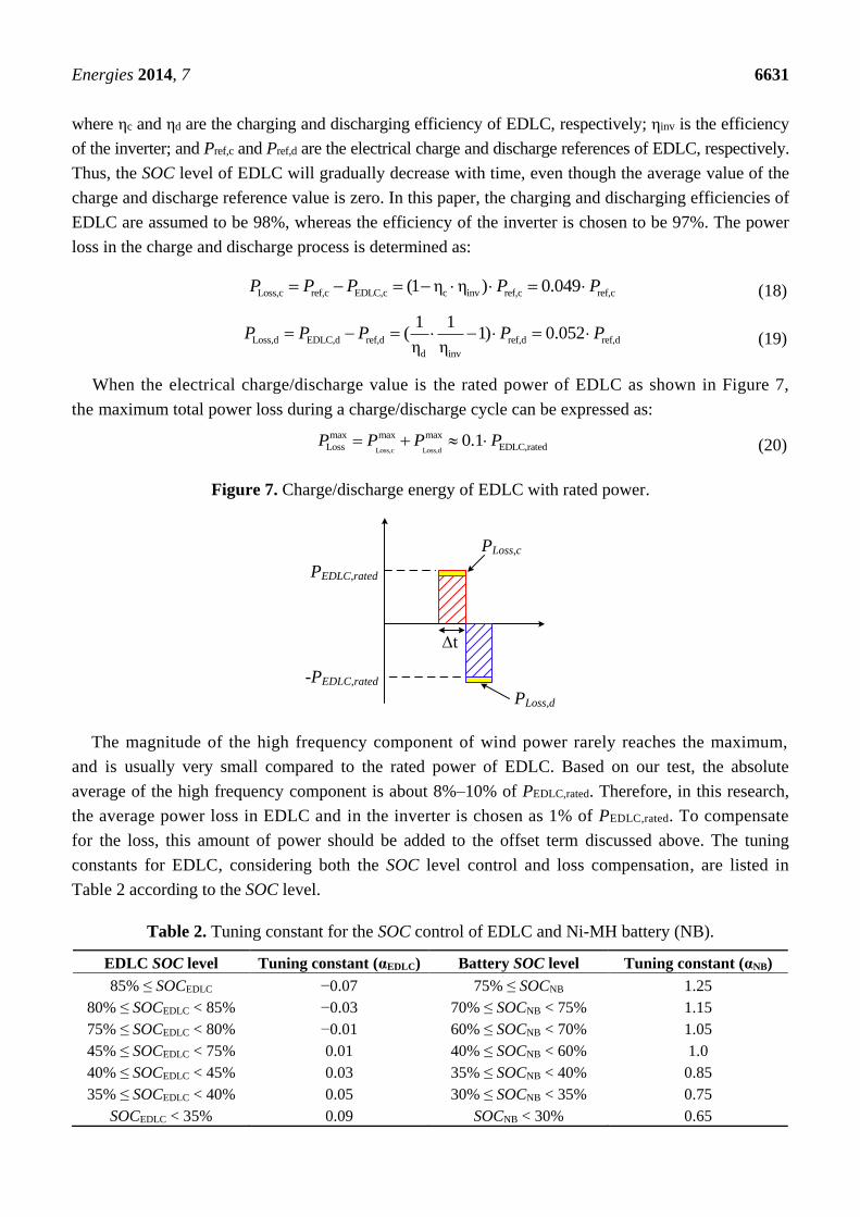
When the electrical charge/discharge value is the rated power of EDLC as shown in Figure 7,
the maximum total power loss during a charge/discharge cycle can be expressed as:
Loss,c Loss,d
max max max
Loss EDLC,rated0.1P P P P (20)
Figure 7. Charge/discharge energy of EDLC with rated power.
The magnitude of the high frequency component of wind power rarely reaches the maximum,
and is usually very small compared to the rated power of EDLC. Based on our test, the absolute
average of the high frequency component is about 8%–10% of PEDLC,rated. Therefore, in this research,
the average power loss in EDLC and in the inverter is chosen as 1% of PEDLC,rated. To compensate
for the loss, this amount of power should be added to the offset term discussed above. The tuning
constants for EDLC, considering both the SOC level control and loss compensation, are listed in
Table 2 according to the SOC level.
Table 2. Tuning constant for the SOC control of EDLC and Ni-MH battery (NB).
EDLC SOC level Tuning constant (αEDLC) Battery SOC level Tuning constant (αNB)
85% ≤ SOCEDLC −0.07 75% ≤ SOCNB 1.25
80% ≤ SOCEDLC < 85% −0.03 70% ≤ SOCNB < 75% 1.15
75% ≤ SOCEDLC < 80% −0.01 60% ≤ SOCNB < 70% 1.05
45% ≤ SOCEDLC < 75% 0.01 40% ≤ SOCNB < 60% 1.0
40% ≤ SOCEDLC < 45% 0.03 35% ≤ SOCNB < 40% 0.85
35% ≤ SOCEDLC < 40% 0.05 30% ≤ SOCNB < 35% 0.75
SOCEDLC < 35% 0.09 SOCNB < 30% 0.65
PEDLC,rated
-PEDLC,rated
Dt
PLoss,c
PLoss,d
Energies 2014, 7 6632
3.2.2. State-of-Charge Control Strategy of the Ni-MH Battery
The main concept of the SOC control strategy for NB is similar to that of EDLC. However, in this case,
the NB inverter reference is not directly modified. Instead, the system output reference of the next
10-min period is adjusted according to the change of the NB SOC level. If the SOC level is above
the maximum safe range, the system output reference should be increased so that the discharge power
is increased. On the contrary, when the SOC level is very low, the SOC level can be increased or less
reduced by decreasing the system output reference. For this, the low frequency component at time t
(A
tP ) is multiplied by a different tuning constant depending on the NB SOC level as follows:
A_new ANBαt tP P (21)
The tuning constant αNB used in the research is summarized in Table 2. It should be noted that the
tuning constant for a safe range (40%–60% in this research) is unity, not zero.
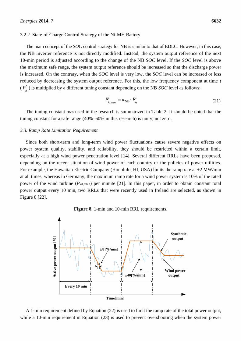
3.3. Ramp Rate Limitation Requirement
Since both short-term and long-term wind power fluctuations cause severe negative effects on
power system quality, stability, and reliability, they should be restricted within a certain limit,
especially at a high wind power penetration level [14]. Several different RRLs have been proposed,
depending on the recent situation of wind power of each country or the policies of power utilities.
For example, the Hawaiian Electric Company (Honolulu, HI, USA) limits the ramp rate at ±2 MW/min
at all times, whereas in Germany, the maximum ramp rate for a wind power system is 10% of the rated
power of the wind turbine (Pwt,rated) per minute [21]. In this paper, in order to obtain constant total
power output every 10 min, two RRLs that were recently used in Ireland are selected, as shown in
Figure 8 [22].
Figure 8. 1-min and 10-min RRL requirements.
Every 10 min
± 8[%/min]
±40[%/min]
Time [min]
Act
ive
po
wer
ou
tpu
t [
%]
Synthetic
output
Wind power
output
A 1-min requirement defined by Equation (22) is used to limit the ramp rate of the total power output,
while a 10-min requirement in Equation (23) is used to prevent overshooting when the system power

Energies 2014, 7 6633
reference is changed. Here, the term k is used to count the change of the system reference every 10 min,
whereas the term t represents a 1-s change of system reference:
1sys, ref sys, ref wt, rated
10 08
60
t tP P . P (22)
1sys, ref sys, ref wt, rated0 4k kP P . P (23)
4. Simulation Studies
4.1. Configuration of the Test System
The wind-HESS test system shown in Figure 1 is implemented in the RSCAD environment.
A Vestas V82 wind turbine model provided in the RSCAD library is used to cooperate with the
NB-EDLC HESS. The rated power of the wind turbine is 1.65 MW. Two different wind power output
profiles for 2 h (7200 s) shown in Figure 9 are used in the simulations.
Figure 9. Active power output of wind turbine sampled at 1-s resolution: (a) Wind Pattern 1;
and (b) Wind Pattern 2.
(a)
(b)
The capacities of the storage are chosen based on the selected energy management algorithm.
The rating of the NB is determined to continuously supply or store 60% of the wind turbine rated
power for approximately 600 s. The rating of EDLC is chosen so that it can supply or store 40% of the
wind turbine rated power for 60 s. The SOC limits and some operational margins are also considered to
determine the ratings of the storage. The detail parameters of the test system are summarized in
Table 3.
0 1200 2400 3600 4800 6000 72000
0.5
1
1.5
2
Time(s)
PWT(MW)
0 1200 2400 3600 4800 6000 72000
0.5
1
1.5
2
Time(s)
PWT(MW)

Energies 2014, 7 6634
Table 3. Test system parameters.
Component Parameter Value
Wind turbine Pwt,rated 1.65 MW
NB PNB,rated 1.0 MW
ENB,rated 0.305 MW·h
EDLC PEDLC,rated 0.66 MW
EEDLC,rated 0.022 MW·h
The proposed RWEMA including the DWT algorithm is implemented as a UDM by using the
component builder in the RSCAD. In order to satisfy the typical time step (50 µs) of real-time
simulation and to reduce the size of the computation, the length of MWF was selected as n = 16.
The length of the short-symmetric extension Δt was 4. The decomposition level of DWT was 5,
with “Haar” wavelet function [23]. To test the effectiveness of the SOC control strategy, the initial
SOC levels of NB and EDLC were set at 50%.
4.2. Case 1: Without State-of-Charge Control Strategy
In this case, we applied the proposed RWEMA without the SOC control strategies; i.e., no adjustment
was applied to the EDLC and NB inverter references, regardless of their SOC level. In addition, it is
assumed that the NB and EDLC are disconnected if the SOC level is outside the safe operating limits.
As shown in Figure 10, the total system power output was successfully denoised and flattened with
the help of HESS until the SOC level of EDLC reached its minimum limit (30%) at 3203 s.
Subsequently, even though the short-term fluctuation was included in the system output, the average
output of the system was more flattened than the original wind power output. After 5706 s, when the
SOC level of NB reached its lower limit, the denoising and flattening effects were no longer present
and the total power output fluctuation was the same as that of the original wind turbine power output.
Figure 10. Simulation results for Case 1—without SOC control strategy: (a) total system
power output; and (b) SOC level of EDLC and NB.
(a)
(b)
0 1200 2400 3600 4800 6000 72000
0.5
1
1.5
2
Time(s)
PSYS(MW)
without HESSwithout EDLCwith HESS
0 1200 2400 3600 4800 6000 72000
20
40
60
Time(s)
SOC(%)
EDLC SOC
NB SOC
Energies 2014, 7 6635
4.3. Case 2: With State-of-Charge Control Strategy and Comparison with Simple Moving Average
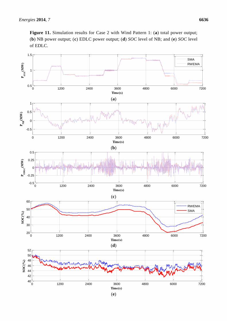
In this case, full RWEMA including the SOC control strategy was applied, while the other
simulation settings were the same as those for Case 1. The simulation results are represented by
blue lines in Figure 11. As shown in Figure 11a, the fluctuation of the wind power output was almost
completely eliminated. Moreover, the total power output was kept constant during each 10-min period
after the linear ramp up/down in the beginning, which demonstrates that the RRL requirements have
been met. The SOC profiles of the NB and EDLC are shown in Figure 11d,e, respectively. It is shown
that the SOC of HESS could be adaptively maintained within the safe operating limits with the
proposed SOC control strategies.
In addition, we implemented a SMA filtering based method and compared the performance with the
proposed wavelet transform based algorithm. The simulation results with SMA are represented by red
lines in Figure 11. Although the basic requirements could be achieved with the SMA based method,
the short term fluctuation remaining in the system output was larger than the results of the
RWEMA case. As shown in Figure 11b,c, the differences in the output of the NB and EDLC between
the two methods were not significant. However, the accumulated effects of the differences were
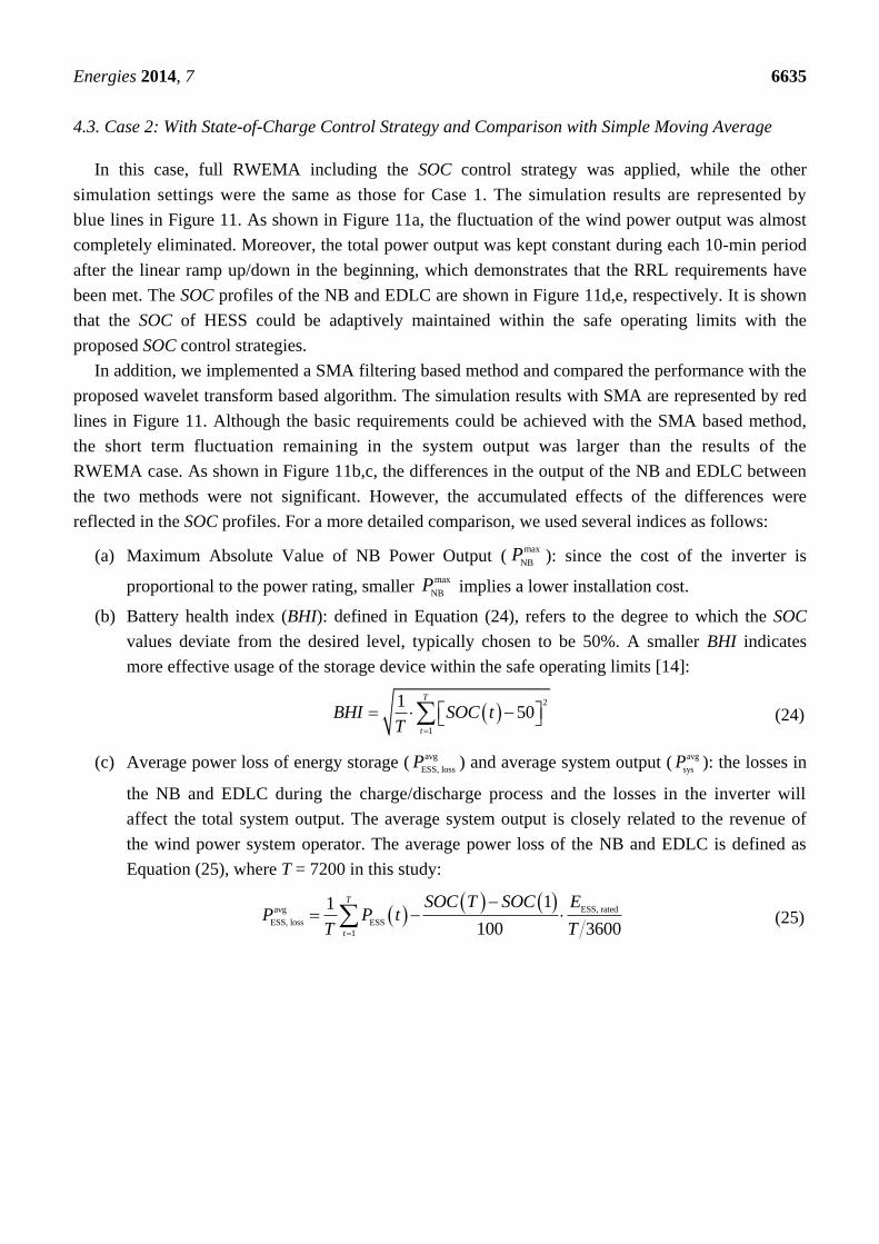
reflected in the SOC profiles. For a more detailed comparison, we used several indices as follows:
(a) Maximum Absolute Value of NB Power Output (max
NBP ): since the cost of the inverter is
proportional to the power rating, smaller max
NBP implies a lower installation cost.
(b) Battery health index (BHI): defined in Equation (24), refers to the degree to which the SOC
values deviate from the desired level, typically chosen to be 50%. A smaller BHI indicates
more effective usage of the storage device within the safe operating limits [14]:
2
1
150
T
t
BHI SOC tT
(24)
(c) Average power loss of energy storage (avg
ESS, lossP ) and average system output (
avg
sysP ): the losses in
the NB and EDLC during the charge/discharge process and the losses in the inverter will
affect the total system output. The average system output is closely related to the revenue of
the wind power system operator. The average power loss of the NB and EDLC is defined as
Equation (25), where T = 7200 in this study:
ESS, ratedavg
ESS, loss ESS
1
11
100 3600
T
t
SOC T SOC EP P t
T T
(25)
Energies 2014, 7 6636
Figure 11. Simulation results for Case 2 with Wind Pattern 1: (a) total power output;
(b) NB power output; (c) EDLC power output; (d) SOC level of NB; and (e) SOC level
of EDLC.
(a)
(b)
(c)
(d)
(e)
0 1200 2400 3600 4800 6000 72000.5
1
1.5
Time(s)
PSYS(MW)
SMA
RWEMA
0 1200 2400 3600 4800 6000 7200
-0.5
0
0.5
1
Time(s)
PNB(MW)
0 1200 2400 3600 4800 6000 7200-0.5
-0.25
0
0.25
0.5
Time(s)
PEDLC(MW)
0 1200 2400 3600 4800 6000 720020
30
40
50
60
Time(s)
SOC(%)
RWEMA
SMA
0 1200 2400 3600 4800 6000 720040
42
44
46
48
50
52
Time(s)
SOC(%)
Energies 2014, 7 6637
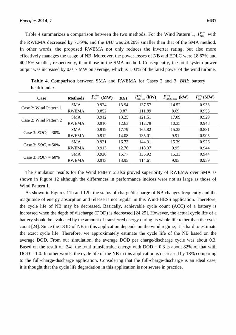
Table 4 summarizes a comparison between the two methods. For the Wind Pattern 1, max
NBP with
the RWEMA decreased by 7.79%, and the BHI was 29.20% smaller than that of the SMA method.
In other words, the proposed RWEMA not only reduces the inverter rating, but also more
effectively manages the usage of NB. Moreover, the power losses of NB and EDLC were 18.67% and
40.15% smaller, respectively, than those in the SMA method. Consequently, the total system power
output was increased by 0.017 MW on average, which is 1.03% of the rated power of the wind turbine.
Table 4. Comparison between SMA and RWEMA for Cases 2 and 3. BHI: battery
health index.
Case Methods max
NBP (MW) BHI
avg
NB, lossP (kW)
avg
EDLC, lossP (kW)
avg
sysP (MW)
Case 2: Wind Pattern 1 SMA 0.924 13.94 137.57 14.52 0.938
RWEMA 0.852 9.87 111.89 8.69 0.955
Case 2: Wind Pattern 2 SMA 0.912 13.25 121.51 17.09 0.929
RWEMA 0.910 12.63 112.78 10.35 0.943
Case 3: SOC0 = 30% SMA 0.919 17.79 165.82 15.35 0.881
RWEMA 0.912 14.08 135.01 9.91 0.905
Case 3: SOC0 = 50% SMA 0.921 16.72 144.31 15.39 0.926
RWEMA 0.913 12.76 118.37 9.95 0.944
Case 3: SOC0 = 60% SMA 0.920 15.77 135.92 15.33 0.944
RWEMA 0.913 13.95 114.61 9.95 0.959
The simulation results for the Wind Pattern 2 also proved superiority of RWEMA over SMA as
shown in Figure 12 although the differences in performance indices were not as large as those of
Wind Pattern 1.
As shown in Figures 11b and 12b, the status of charge/discharge of NB changes frequently and the
magnitude of energy absorption and release is not regular in this Wind-HESS application. Therefore,
the cycle life of NB may be decreased. Basically, achievable cycle count (ACC) of a battery is
increased when the depth of discharge (DOD) is decreased [24,25]. However, the actual cycle life of a
battery should be evaluated by the amount of transferred energy during its whole life rather than the cycle
count [24]. Since the DOD of NB in this application depends on the wind regime, it is hard to estimate
the exact cycle life. Therefore, we approximately estimate the cycle life of the NB based on the
average DOD. From our simulation, the average DOD per charge/discharge cycle was about 0.3.
Based on the result of [24], the total transferrable energy with DOD = 0.3 is about 82% of that with
DOD = 1.0. In other words, the cycle life of the NB in this application is decreased by 18% comparing
to the full-charge-discharge application. Considering that the full-charge-discharge is an ideal case,
it is thought that the cycle life degradation in this application is not severe in practice.

Energies 2014, 7 6638
Figure 12. Simulation results for Case 2 with Wind Pattern 2: (a) total power output;
(b) NB power output; (c) EDLC power output; (d) SOC level of NB; and (e) SOC level
of EDLC.
(a)
(b)
(c)
(d)
(e)
0 1200 2400 3600 4800 6000 72000
0.5
1
1.5
Time(s)
PSYS(MW)
SMA
RWEMA
0 1200 2400 3600 4800 6000 7200-1
-0.5
0
0.5
1
Time(s)
PNB(MW)
0 1200 2400 3600 4800 6000 7200-0.5
-0.25
0
0.25
0.5
Time(s)
PEDLC(MW)
0 1200 2400 3600 4800 6000 720020
40
60
80
Time(s)
SOC(%)
SMA
RWEMA
0 1200 2400 3600 4800 6000 720040
45
50
55
Time(s)
SOC(%)
Energies 2014, 7 6639
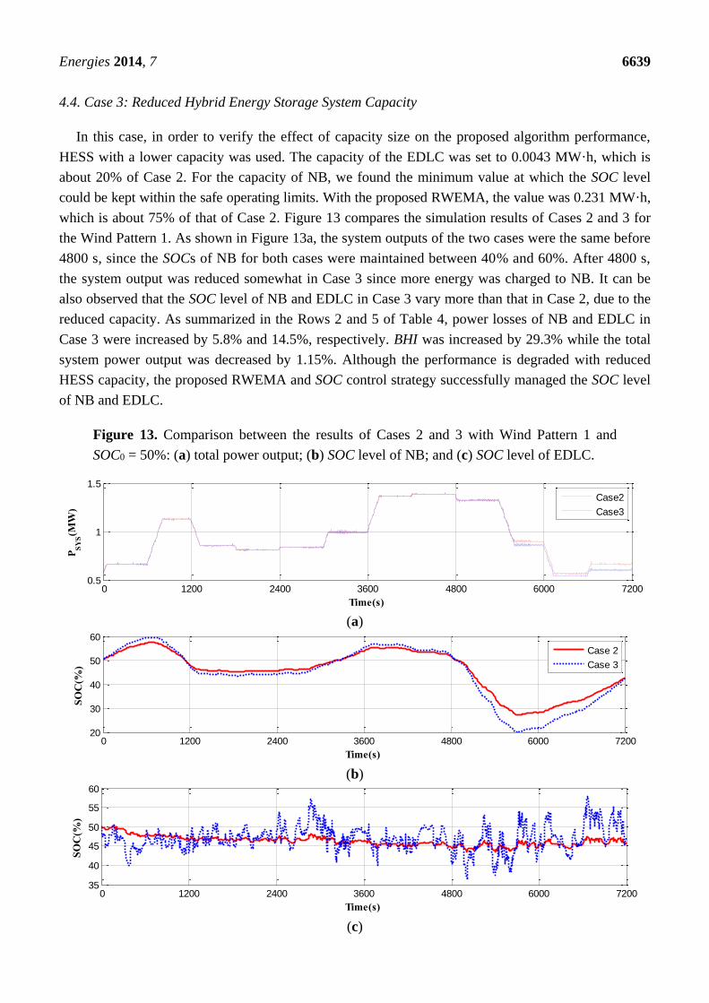
4.4. Case 3: Reduced Hybrid Energy Storage System Capacity
In this case, in order to verify the effect of capacity size on the proposed algorithm performance,
HESS with a lower capacity was used. The capacity of the EDLC was set to 0.0043 MW·h, which is
about 20% of Case 2. For the capacity of NB, we found the minimum value at which the SOC level
could be kept within the safe operating limits. With the proposed RWEMA, the value was 0.231 MW·h,
which is about 75% of that of Case 2. Figure 13 compares the simulation results of Cases 2 and 3 for
the Wind Pattern 1. As shown in Figure 13a, the system outputs of the two cases were the same before
4800 s, since the SOCs of NB for both cases were maintained between 40% and 60%. After 4800 s,
the system output was reduced somewhat in Case 3 since more energy was charged to NB. It can be
also observed that the SOC level of NB and EDLC in Case 3 vary more than that in Case 2, due to the
reduced capacity. As summarized in the Rows 2 and 5 of Table 4, power losses of NB and EDLC in
Case 3 were increased by 5.8% and 14.5%, respectively. BHI was increased by 29.3% while the total
system power output was decreased by 1.15%. Although the performance is degraded with reduced
HESS capacity, the proposed RWEMA and SOC control strategy successfully managed the SOC level
of NB and EDLC.
Figure 13. Comparison between the results of Cases 2 and 3 with Wind Pattern 1 and
SOC0 = 50%: (a) total power output; (b) SOC level of NB; and (c) SOC level of EDLC.
(a)
(b)
(c)
0 1200 2400 3600 4800 6000 72000.5
1
1.5
Time(s)
PSYS(MW)
Case2
Case3
0 1200 2400 3600 4800 6000 720020
30
40
50
60
Time(s)
SOC(%)
Case 2
Case 3
0 1200 2400 3600 4800 6000 720035
40
45
50
55
60
Time(s)
SOC(%)
Energies 2014, 7 6640
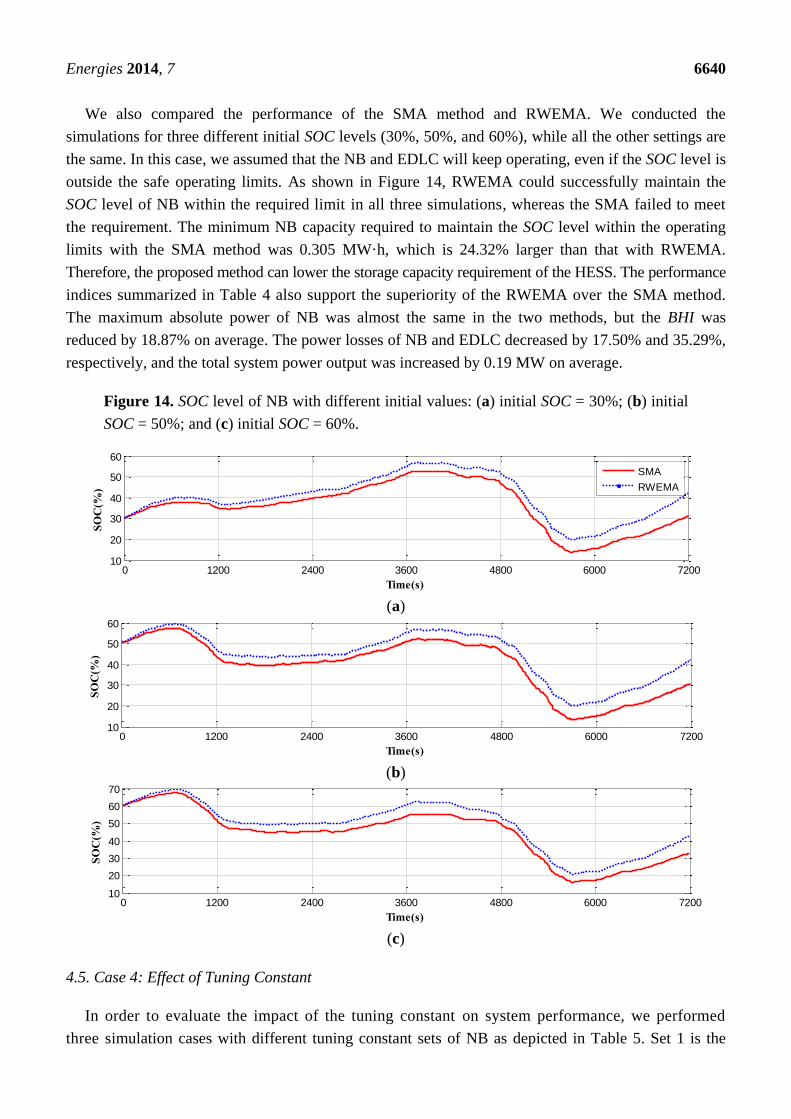
We also compared the performance of the SMA method and RWEMA. We conducted the
simulations for three different initial SOC levels (30%, 50%, and 60%), while all the other settings are
the same. In this case, we assumed that the NB and EDLC will keep operating, even if the SOC level is
outside the safe operating limits. As shown in Figure 14, RWEMA could successfully maintain the
SOC level of NB within the required limit in all three simulations, whereas the SMA failed to meet
the requirement. The minimum NB capacity required to maintain the SOC level within the operating
limits with the SMA method was 0.305 MW·h, which is 24.32% larger than that with RWEMA.
Therefore, the proposed method can lower the storage capacity requirement of the HESS. The performance
indices summarized in Table 4 also support the superiority of the RWEMA over the SMA method.
The maximum absolute power of NB was almost the same in the two methods, but the BHI was
reduced by 18.87% on average. The power losses of NB and EDLC decreased by 17.50% and 35.29%,
respectively, and the total system power output was increased by 0.19 MW on average.
Figure 14. SOC level of NB with different initial values: (a) initial SOC = 30%; (b) initial
SOC = 50%; and (c) initial SOC = 60%.
(a)
(b)
(c)
4.5. Case 4: Effect of Tuning Constant
In order to evaluate the impact of the tuning constant on system performance, we performed
three simulation cases with different tuning constant sets of NB as depicted in Table 5. Set 1 is the
0 1200 2400 3600 4800 6000 720010
20
30
40
50
60
Time(s)
SOC(%)
SMA
RWEMA
0 1200 2400 3600 4800 6000 720010
20
30
40
50
60
Time(s)
SOC(%)
0 1200 2400 3600 4800 6000 720010
20
30
40
50
60
70
Time(s)
SOC(%)

Energies 2014, 7 6641
reference case; the gap between the consecutive tuning constants was doubled in Set 2, while the gap
was halved in Set 3. The other simulation settings, including the tuning constant of EDLC, were kept
the same as those in Case 3.
Table 5. NB tuning constant sets used in Case 4.
Battery SOC Level Tuning constant (αNB)
Set 1 Set 2 Set 3
75% ≤ SOCNB 1.25 1.55 1.10
70% ≤ SOCNB < 75% 1.15 1.35 1.05
60% ≤ SOCNB < 70% 1.05 1.15 1.00
40% ≤ SOCNB < 60% 1.00 1.00 1.00
35% ≤ SOCNB < 40% 0.85 0.75 0.90
30% ≤ SOCNB < 35% 0.75 0.55 0.85
SOCNB < 30% 0.65 0.35 0.80
The results are shown in Figure 15 and the performance indices are summarized in Table 6. The
maximum absolute power of NB and the loss of HESS were the smallest in Case 3, while the BHI was
the smallest in Case 2. As shown in Figure 15a, the system power output and the SOC profile were
almost the same for three simulation cases before 5600 s. Subsequently, the system output reference
was the lowest in the result with Set 2, since the tuning constant of Set 2 is the smallest for low
SOC levels. Therefore, the magnitude of charging power would be the maximum in the results with
Set 2. As a result, the power loss of NB was the most increased. On the other hand, the recovery of the
SOC level with Set 3 was the slowest. Furthermore, in the simulation with Set 3, the SOC level was
less than the low operating limit, as shown in Figure 15b. Therefore, the value of the tuning constant
should be selected carefully considering the tradeoff between the loss and the effectiveness of the
NB usage.
Figure 15. Simulation results for Case 4 with different tuning constant sets: (a) total system
power output; and (b) SOC level of NB.
(a)
(b)
0 1200 2400 3600 4800 6000 72000
0.5
1
1.5
Time(s)
PSYS(MW)
Set1
Set2
Set3
0 1200 2400 3600 4800 6000 720010
20
30
40
50
60
Time(s)
SOC(%)
19
20
21
22

Energies 2014, 7 6642
Table 6. Impact of tuning constant to system performance.
Tuning constant set max
NBP (MW) BHI
avg
NB, lossP (kW)
avg
sysP (MW)
Set 1 0.913 12.76 118.37 0.944
Set 2 0.997 11.75 147.29 0.906
Set 3 0.799 13.51 102.04 0.967
5. Conclusions
This paper proposed a novel RWEMA of a wind-HESS system to denoise and flatten the wind
power output. A real-time DWT was used to decompose the 1-s sampled wind power output into
high-frequency and low-frequency components. The high-frequency components were used as a
reference of the EDLC, while the low-frequency terms were used to calculate the reference of the NB.
SOC control strategies of EDLC and NB were also proposed by using the tuning constant concept.
In addition, 1-min and 10-min RRL requirements can be met by the proposed RWEMA.
The simulation models of the NB and EDLC energy storage system were developed in the
RTDS/RSCAD software. A configuration interface was also developed to modify the simulation
parameters of the model. The proposed RWEMA has been tested in real-time by using the RTDS
hardware and software. The simulation results demonstrated the effectiveness of the proposed control
algorithm in denoising and flattening wind power output, and managing the SOC level of storage.
The results also showed that the required capacity ratings of storage used in RWEMA were smaller
than those of the conventional SMA-based technique. Since the proposed approach uses a simple
DWT-based structure without any prediction technique, it can be easily implemented in real-time
applications. In order to move beyond the simulation level and into the hardware implementation,
many practical issues and requirements still need to be considered, such as data acquisition,
communication media and protocol, data management, and selection of processor. The proposed
method will be implemented as an actual hardware controller and be tested with the real Wind-HESS
system in the future.
Acknowledgments
This work was partially supported by Korea Institute of Energy Technology Evaluation and
Planning (KETEP) grant funded by Korea Government Ministry of Trade, Industry and Energy
(No. 20123010020080). This work was also partially supported by the National Research Foundation
of Korea (NRF) grant funded by the Korea Government (MSIP) (No. 2010-0028509).
Author Contributions
Tran Thai Trung developed the simulation models and wrote the first draft of the paper. Tran Thai Trung
and Seok-Il Go completed the simulation. Joon-Ho Choi and Soon-Ryul Nam discussed the results
and implications, and commented on the manuscript. Seon-Ju Ahn coordinated the main theme of
this paper, and thoroughly reviewed and edited the manuscript. All the authors read and approved the
final manuscript.

Energies 2014, 7 6643
Conflicts of Interest
The authors declare no conflict of interest.
References
1. Fox, B. Introduction. In Wind Power Integration: Connection and System Operational Aspects;
The Institution of Engineering and Technology (IET): London, UK, 2007; pp. 14–18.
2. Zhang, J.; Cheng, M.; Chen, Z.; Fu, X. Pitch angle control for variable speed wind turbines. In
Proceedings of the Third International Conference on Electric Utility Deregulation and
Restructuring and Power Technologies, DRPT 2008, Nanjing, China, 6–9 April 2008; pp. 2691–2696.
3. Abedini, A.; Nasiri, A. Output power smoothing for wind turbine permanent magnet synchronous
generators using rotor inertia. Electr. Power Compon. Syst. 2008, 37, 1–19.
4. Barton, J.P.; Infield, D.G. Energy storage and its use with intermittent renewable energy.
IEEE Trans. Energy Convers. 2004, 19, 441–448.
5. Abbey, C.; Joos, G. Supercapacitor energy storage for wind energy applications. IEEE Trans.
Ind. Appl. 2007, 43, 769–776.
6. Ushiwata, K.; Shishido, S.; Takahashi, R.; Murata, T.; Tamura, J. Smoothing control of wind
generator output fluctuation by using electric double layer capacitor. In Proceedings of
the International Conference on Electrical Machines and Systems (ICEMS), Seoul, Korea,
8–11 October 2007; pp. 308–313.
7. Tanabe, T.; Sato, T.; Tanikawa, R.; Aoki, I.; Funabashi, T.; Yokoyama, R. Generation scheduling
for wind power generation by storage battery system and meteorological forecast. In Proceedings of
the 2008 IEEE Power and Energy Society General Meeting—Conversion and Delivery of
Electrical Energy in the 21st Century, Pittsburgh, PA, USA, 20–24 July 2008; pp. 1–7.
8. Sheikh, M.R.I.; Muyeen, S.M.; Takahashi, R.; Murata, T.; Tamura, J. Minimization of fluctuations
of output power and terminal voltage of wind generator by using STATCOM/SMES.
In Proceedings of the 2009 IEEE Bucharest PowerTech, Bucharest, Romania, 28 June–2 July 2009;
pp. 1–6.
9. Yoshimoto, K.; Nanahara, T.; Koshimizu, G. New control method for regulating state-of-charge of
a battery in hybrid wind power/battery energy storage system. In Proceedings of the 2006
IEEE PES Power Systems Conference and Exposition, PSCE '06, Atlanta, GA, USA,
29 October–1 November 2006; pp. 1244–1251.
10. Li, W.; Joós, G.; Bélanger, J. Real-time simulation of a wind turbine generator coupled with a
battery supercapacitor energy storage system. IEEE Trans. Ind. Electron. 2010, 57, 1137–1145.
11. Suvire, G.O.; Mercado, P. Active power control of a flywheel energy storage system for wind
energy applications. IET Renew. Power Gener. 2012, 6, 9–16.
12. Mishra, Y.; Mishra, S.; Li, F. Coordinated tuning of DFIG-based wind turbines and batteries
using bacteria foraging technique for maintaining constant grid power output. IEEE Syst. J. 2012, 6,
16–26.
13. Li, X.; Li, Y.; Han, X.; Hui, D. Application of fuzzy wavelet transform to smooth wind/PV hybrid
power system output with battery energy storage system. Energy Procedia 2011, 12, 994–1001.

Energies 2014, 7 6644
14. Jiang, Q.; Hong, H. Wavelet-based capacity configuration and coordinated control of hybrid
energy storage system for smoothing out wind power fluctuations. IEEE Trans. Power Syst. 2013,
28, 1363–1372.
15. Xia, R.; Meng, K.; Qian, F.; Wang, Z.-L. Online wavelet denoising via a moving window.
Acta Autom. Sin. 2007, 33, 897–901.
16. RTDS Technologies. Power System Simulator Hardware. Available online: http://rtds.com/hardware/
hardware.html (accessed on 30 May 2014).
17. Omar, N.; Daowd, M.; Hegazy, O.; Bossche, P.V.D.; Coosemans, T.; Mierlo, J.V. Electrical
double-layer capacitors in hybrid topologies—Assessment and evaluation of their performance.
Energies 2012, 5, 4533–4568.
18. Oldham, K.B. A Gouy-Chapman-Stern model of the double layer at a (metal)/(ionic liquid)
interface. J. Electroanal. Chem. 2008, 613, 131–138.
19. MathWorks. Implement Generic Supercapacitor Model—Simulink. Available online: http://www.
mathworks.com/help/physmod/sps/powersys/ref/supercapacitor.html (accessed on 3 June 2014).
20. Tremblay, O.; Dessaint, L.-A.; Dekkiche, A.-I. A generic battery model for the dynamic
simulation of hybrid electric vehicles. In Proceedings of the IEEE Vehicle Power and Propulsion
Conference, VPPC 2007, Arlington, TX, USA, 9–12 September 2007; pp. 284–289.
21. Gevorgian, V.; Booth, S. Review of Prepa Technical Requirements for Interconnecting Wind and
Solar Generation; National Renewable Energy Laboratory: Golden, CO, USA, 2013.
22. Fox, B. Operation of power systems. In Wind Power Integration: Connection and System
Operational Aspects; The Institution of Engineering and Technology (IET): London, UK, 2007;
pp. 160–170.
23. Chan, F.-P.; Fu, A.-C.; Yu, C. Haar wavelets for efficient similarity search of time-series: With and
without time warping. IEEE Trans. Knowl. Data Eng. 2003, 15, 686–705.
24. Han, S.; Han, S. Economic feasibility of V2G frequency regulation in consideration of battery wear.
Energies 2013, 6, 748–765.
25. Peterson, S.B.; Apt, J.; Whitacre, J. Lithium-ion battery cell degradation resulting from realistic
vehicle and vehicle-to-grid utilization. J. Power Sources 2010, 195, 2385–2392.
© 2014 by the authors; licensee MDPI, Basel, Switzerland. This article is an open access article
distributed under the terms and conditions of the Creative Commons Attribution license
(http://creativecommons.org/licenses/by/4.0/).