Notice of Public Meeting San Diego River Conservancy

A public meeting of the Governing Board of

The San Diego River Conservancy will be held Thursday,

September 8, 2016 2:00 pm – 4:00 pm

Meeting Location County of San Diego Administration Center (CAC)

1600 Pacific Highway, Room 302 San Diego, California 92101

Tele-Conference Locations

Natural Resources Agency Department of Finance 1416 Ninth Street, Room #1311 State Capitol, Room 1145

Sacramento, CA 95814 Sacramento, CA 95814

Contact: Wendell Taper (619) 645-3183

Meeting Agenda The Board may take agenda items out of order to accommodate speakers and to maintain a quorum, unless noted as time specific.

1. Roll Call

2. Approval of Minutes (ACTION)

Consider approval of minutes for the July 14th, 2016 meeting. 3. Public Comment (INFORMATIONAL)

Any person may address the Governing Board at this time regarding any matter within the Board’s authority. Presentations will be limited to three minutes for individuals and five minutes for representatives of organizations. Submission of information in writing is encouraged. The Board is prohibited by law from taking any action on matters that are discussed that are not on the agenda; no adverse conclusions should be drawn by the Board’s not responding to such matters or public comments.

4. Chairperson’s and Governing Board Members’ Report (INFORMATIONAL/ ACTION)

5. Deputy Attorney General Report (INFORMATIONAL/ACTION)

6. Proposition 1 Grant Program – update (INFORMATIONAL/ ACTION)

Discussion of the San Diego River Conservancy Proposition 1, Round 1 grants and Round 2’s concept proposals.

Discussion: Julia Richards, SDRC Executive Officer

7. Flume Trail Extension Project (INFORMATIONAL)

Design and construction of a 0.8 mile trail segment of the San Diego River Trail (Gap 59) and trailhead on property owned by Helix Water District. This project was completed with support from the following partners: California Natural Resources Agency, San Diego River Conservancy, The San Diego Foundation (Hervey Family of Funds), County of San Diego, Department of Parks and Recreation and Helix Water District.

Presentation: Jill Bankston, County of San Diego

8. San Diego County Trans County Trail (INFORMATIONAL/ACTION)

The County of San Diego’s Park and Recreation summary of the history, progress and establishment of a planning committee for the Trans County Trail program.

Presentation: Lorrie Bradley, County of San Diego

9. Ecological Limits of Hydrologic Alteration (ELOHA) (INFORMATIONAL/

ACTION)

Presentation on report entitled, “Application of Regional Flow-ecology to Inform Management Decision in the San Diego River Watershed – Draft”. This project illustrates how varying hydrological flows affect aquatic biology over time in the San Diego River watershed. Presentation: Dr. Eric Stein, Southern California Coastal Water Research Project

10. Executive Officer’s Report (INFORMATIONAL / ACTION)

The following topics may be included in the Executive Officer’s Report. The Board may take action regarding any of them:

• Trust for Public Land • Department of General Services – Contracted Fiscal Services

• Strategic Plan update 2018-2023 11. Next Meeting

The next scheduled board meeting will be held Thursday, November 10th, 2016, 2:00 - 4:00 p.m. 12. Adjournment

Accessibility

If you require a disability related modification or accommodation to attend or participate in this meeting, including auxiliary aids or services, please call Wendell Taper at 619-645-3183 or Julia Richards at 619-645-3188.

State of California San Diego River Conservancy

Meeting of September 8, 2016

ITEM: 1 SUBJECT: ROLL CALL AND INTRODUCTIONS

State of California San Diego River Conservancy

Meeting of September 8, 2016 ITEM: 2

SUBJECT: APPROVAL OF MINUTES (ACTION)

The Board will consider adoption of the July 14, 2016 public meeting minutes.

PURPOSE: The minutes of the Board Meeting are attached for

review. RECOMMENDATION: Approve minutes

SAN DIEGO RIVER CONSERVANCY

Minutes of July 14, 2016 Public Meeting

(Draft Minutes for Approval on September 8, 2016)

CONSERVANCY Board Chair, Ben Clay called the July 14, 2016 meeting of the San Diego River Conservancy to order at approximately 2:00 p.m.

1. Roll Call Members Present Bryan Cash Natural Resources Agency, Alternate Designee (via phone) Brent Eidson Mayor, City of San Diego, Designee Dianne Jacob Supervisor, County of San Diego, Second District Ben Clay, Chair Public at Large Ruth Hayward Public at Large Deanna Spehn Speaker of the Assembly, Appointment John Donnelly Wildlife Conservation Board Andrew Poat Public at Large (arrived 2:15pm) Ann Haddad Public at Large Gary Strawn San Diego Regional Water Quality Control Board Robin Greene Department of Parks and Recreation Kari Krogseng Department of Finance (Via Phone) Absent Scott Sherman Councilmember, City of San Diego, District 7 Staff Members Present

Julia Richards Executive Officer Wendell Taper Administrative Services Manager Dustin Harrison Environmental Scientist Hayley Peterson Deputy Attorney General

Ben Clay we’ve got a quorum.

2. Approval of Minutes Ben Clay asked if there was a motion for approval of the minutes. Dianne Jacob moved for approval of the minutes for the March 10 meeting and Brent Eidson seconded. Roll Call: (6-0-2), Ayes: Brent Eidson, Deanna Spehn, Kari Krogseng, Bryan Cash, Dianne Jacob, Ben Clay,

Ruth Hayward. (Abstain: Robin Greene, Ann Haddad) 3. Public Comment (INFORMATIONAL) Ben Clay I don’t have any general public comment, but I do have a slip from Jim Peugh for Item number 6 when that comes up. Any other comments?

4. Chairperson’s and Governing Board Members’ Report (INFORMATIONAL/ACTION)

Ben Clay stated it’s good to have the Executive Officer back. She’s been rather busy over the last couple of months with the new addition to her family.

Ben Clay noted me met with the Chairman of the San Diego County Water Authority former General Manager of Helix Water District just to get caught up on water issues. In addition he walked the beach trail from Old Town to Ocean Beach and stated the trail needs a lot of help. We will work with the City and figure out how to make it better. I don’t like to use the word, but it’s a hazard in the making. Also he walked over by the oil spill area to take a look.

Gary Strawn discussed the results of a fish tissue sampling that San Diego Regional Water Quality Control Board (SDRWQCB) did in various spots of the river almost two years ago. Normally this is an expensive process to show how many people are catching and eating the fish. We had some money left over from another project that we were able to do this. A bunch of volunteers helped California Department of Fish and Wildlife and scientists from the Waterboard collect samples. It was the first time in 17 years since there’d been any sampling. The data collected is compared to various studies done as far back as 1979 through 1999. The short answer is very good. The levels of polychlorinated bisphenyls (PCBs) and dichlorodiphenyltrichloroethane (DDTs) were well below levels of concern. That’s good news. The only two items that showed up are mercury and selenium. We don’t understand what selenium is doing - we’ll have to do more research. The mercury is methyl mercury an airborne contaminant that says all the stuff we were putting into the river we’re not any more or at least to the levels that are getting into the food chain and into the fish. There were several larger bass with detectable levels of mercury, but were less than half 15, 20 years ago. We did a survey of people to see who is catching fish and eating them. People surveyed said they don’t eat fish out of the river. If they want to eat something, they go up and catch them at the reservoir. I want to leave one message, it was really good news. We thought it would be good, but we didn’t think it would be this good.

Ben Clay asked where were the samples taken from?

Gary Strawn responded they went out at the Walker Ponds (Santee) just before it was opened to the public. In two weeks he expects to have a report on the same fish tissue sampling in San Diego Bay to see what kind of contaminates are coming directly from the river. It will be interesting information to see what kind of benefits we see from all the work, money, and energy that’s being spent to clean up the rivers. This is the kinds of information we need to continue support what we’re doing.

Ruth Hayward asked what lake did you catch the fish from?

Gary Strawn responded Lake Jennings and El Capitan. The others like San Vicente are piped in. So we still have those airborne contaminates. There may have been some others.

Ruth Hayward Sounds like Murray might be a good bet, too.

Brent Eidson If I may Mr. Chairman. Since I am from the agency that has nine of those reservoirs and have been working on this issue at the City, I concur with Mr. Strawn’s statements that this is mostly airborne mercury. There are detectable levels, but they don’t appear to be at the levels that are harmful for human consumption. With that being said, many of the reservoirs in the entire region we’re working with the other reservoir keepers to start putting notices up to let people know.

Ben Clay Is this the notice you send out in your service area about various things in the water? Can you take the mercury out during treatment?

Brent Eidson responded, no that is the potable water supply. This is the raw water supply. So what the City of San Diego sends out if the water quality after it has been treated and is potable. I don’t know I believe we do. The issue is its being found in the fish tissue and not in the water supply. It’s coming from air pollutants and accumulated in the fish.

Gary Strawn The State put out a statewide warning two or three years ago all the waters of the state but put the burden on our waters that don’t meet standards.

Ben Clay noted he gave a talk at Serra Museum regarding the Conservancy’s grant for internal and external exhibits. So then when you look at the river it will tell you what you’re looking. The City has been working hard to get facility up to speed for ADA access. The museum has a lot of potential for telling the story of the San Diego River which is what I’m most interested getting the word out. The views from the ocean to the east are phenomenal.

Item 5. Deputy Attorney’s General Report No to report.

Item 6. Diesel Spill over the San Diego River (INFOMRATION) Ben Clay you read about it and heard about it here for those of you in Sacramento you may not have. I thought it would be smart for Executive officer to brief us on what happened. Julia Richards showed an overview of the spill site. Today there will be three speakers to talk about their roles in cleanup effort. First speaker is Kris Weise from California Department of Fish and Wildlife Office of Spill Prevention and Response (OSPR). The second speaker is Kevin Heaton from the County of San Diego Department of Environmental Health Voluntary Assistance Program and the last speaker is Angus McDonald president of the SOCO Group, owner of the truck that overturned. Kris Weise I brought notes because I’m exhausted from doing spill after spill since this one. But am happy to be here and meet the Board. A lot of people don’t know why Wildlife shows up to oil spills. I’m going to talk about the Morena Blvd. incident and the good things that came from it to build on in the future with the Conservancy. He tried to bring synergy how to work these problems in the future. OSPR has recently given a mandate to move inland. OSPR has an outreach program. They take this program to the public. In 1980 there was a big push to address oil spills and OSPR became an agency in 1990. OSPR will be planning for inland responses like along the banks of San Diego River. They draft response plans for those areas and pre-identify where spills might occur and build on those relationships with agencies that have jurisdiction and respond proactively. The program covers authority to address spills on inland and marine areas. They conduct drills and exercises for those environments and have been in the news this week in Mission Bay. They have spill response organizations ready to go and are funded. His supervisor Chris Nixon discussed San Diego River Watershed makes since because it has public use and a lot of people interested on what’s going on. Highway 15 and 5 corridors are likely locations for spills to occur.

Ben Clay stated there’s a fuel tank further up Missions Valley near Qualcomm and have had problems in the past. There’s potential if you look at risk. Kris Weise Those are connected by pipeline to Los Angeles. We are threatened from quite a few locations. The more likely unfortunately would be a tanker truck rollover again. OSPR wants to work with the Conservancy. There was a test 17 years ago high levels of contaminants. We are not the only agency pushing for change. There was a lot of fire people and no water deployed. The areas of scooped soil there was a berm and I don’t know how many thousands of gallons of collected in that location but they took dirt and did a fantastic job. He spoke about other partners. NRC Environmental Services was there and they regularly respond. They were on scene initially before they were called because they monitor for these types of incidents. OSPR developed a plan because there was a lot of diesel and crude oil down there. They improvised sediment impound placed to slow oil. That effort was done under the river and kept oil from migrating back through storm drain. Diesel mostly impacted sediment in river area. The Fire Department had a vacuum suck up the oil. In the morning we had a unified command meeting. Initially he estimated 50 gallons, but hindsight more like 250 gallons moved with winds upstream. If gone downstream, US Fish and Wildlife concerns down to estuary where Least Tern nesting would be catastrophic for wildlife and fishes. There was drainage under the bridge and tons of diesel. NRC used a vacuum hose and mostly gone and clean downstream. OSPR met up in our unified command at parking lot of Metro day two planning to respond and make headway. The river was pretty clean, but some sheen was seen from vegetation. They removed oil, debris and excavation of soil. Vast majority successfully collected with skimmer and actively sweeping oil to boom. Don’t have final numbers of how much dirt was removed. They flagged the area to remove vegetation and thought to remove 6-8 inches. The excavation removed oil by using sniffers to detect and keep digging. The liquid is groundwater. There was some intrusion into groundwater so excavation was improved measure for removing the spill. At the northern end of Morena Blvd. next to Friars Rd. Before the dig and what we ended up with an Olympic sized pool 2-3 feet deep. The pads absorb diesel still floating on the surface. When done, OSPR backfilled and scraped soil from area. United States Army Corp of Engineers said we need to provide it to prevent back pooling. On the south end there is quite a bit of soil removed. That area was heavily vegetated with non-native species. We took those out as part of the plan. Ben Clay how much did all this cost? Kris Weise responded $250,000 would be a drop in the bucket, if it was $500K I wouldn’t be surprised. The soil was trucked to Arizona because landfill disposal there is faster to get done. It takes 16 days to get approved to dump locally and is cheaper to truck out there. They brought clean soil backfill in from Arizona. Dianne Jacob asked who pays? Does the responsible party pay? Kris Weise The trucking company generally has an insurance policy. Some cases they pay first $100 million of response and after that there’s a jumbo insurance policy. OSPR paid for cleanup. He wants to minimize cost to maximize restoration. Ben Clay asked is there a fund you draw from for insurance? What did you learn from this if this happened again? Kris Weise responded when there is a responsible party, our office bills them for our time. He didn’t know the conservancy exists. As you move up the river channel there are other agencies. I don’t know our Native American culture although I know there is a presence.

Ben Clay the river flows down to estuary and enters Mission Bay channel. Is there opportunity to pre-position boom to keep that from entering estuary? Kris Weise Certainly a possibility. In Los Angeles there are a number of places of pre-deployed boom. You don’t typically want those sitting in the river. It is something to consider, though. Julia Richard introduced Kevin Heaton from County of San Diego. Kevin Heaton County of San Diego Department of Environmental Health. He was out there right after it occurred for five days assisting Fish and Wildlife measuring concentrations. Also, informing County overall as to what response was. He is the County representative who deals with meeting the cleanup standards. He was out there during response and established screening levels of soil removal. They use 100 parts per million (ppm) as threshold to look at. It exceeded standard that soil was excavated. After all that, estimation of volume removal is not known. About 1000 cubic yards of soil removed and other vegetation and debris. Of that, we had large numbers of samples - only two samples exceeded standard for field indications. Quick synopsis of what happened. The bridge from north part, ABCD all the way to I. Different parts of bridge were abutments, Sections ABC were where contamination occurred. Weep holes that drained fuel to riverbed on that eastern side of the bridge. Top route soil cleanup levels in terms of analytical. Our goal was 1000 ppm total petroleum hydrocarbons (TPH) for diesel. Various components of diesel. Positive thing is, all individual components were non-detect in almost all samples. Numbers below groundwater where cleanup occurred was 640 micrograms per liter. Those compounds were also non-detect. This shows bridge abutment sections on northern side. On right hand side, south end is DEFG and I. Most contamination that was cleaned was on northern side where holes that drained bridge were plugged. This summary total estimated soil in section A 215 cubic yards (cy) B 185 cy C 210 cy and along river, 63 cy. On south side, only one section H - 208 cy removed. 120 samples taken of soil around that. Only two samples exceeded standard resulted in them going out doing additional excavation. After all work, highest remaining concentration was 650 milligram per kilogram which is 2/3 to the cleanup level (1000) which was effective. This list of water samples. Open excavation with water and absorbent pads were in order of 3000 to 2300 ppt. Two or three weeks after cleanup occurred, consultant did dry samples and sampled groundwater and the highest concentration was 270 – most was non-detect. Ben Clay your samples. Are we in good shape out there? Kevin Heaton responded all samples have shown we are below standards we have established. Only outstanding is what NRC took out and make sure numbers are good. Ben Clay Anything in retrospect that should have happened that didn’t? Kevin Heaton there was good coordination of all agencies. They were out there before emergency call came out. NRC was out there before Fish and Game was there, probably out of the norm, which is good. He provided a handout of all information of background samples. Ben Clay Thank you, I hear the initial response team was well managed. We have SDSU students we’re working with to do testing and monitoring. [No show Angus McDonald, SoCo Group.] Ben Clay thanked all parties involved. He is interested in lessons learned. The Conservancies should spend more time on getting back to state agencies on what can be done to help. This won’t be the last time this happens.

Gary Strawn said there is a cleanup fund. Most money the SDRWQCB gets from fines are pumped back into the community for fixes. Also regional stormwater permits have requirements for not dumping directly into river. Ben Clay introduced Jim Peugh. Jim Peugh Conservation Chair San Diego Audubon Society. He participated in the area contingency plan and worked on coastal cleanup with Coastal Conservancy and OSPR. The Audubon Society supported when legislature considered expanding into inland cleanups. They have no issues with work done, but think there is something left to be done. He watched cleanup and looked around and a lot of vegetation was damaged. Willows and mulefat is prime habitat for least Bell’s vireo an endangered species. Not a lot to mitigate for this damage. He saw 17 dumpsters and a lot was vegetation damaged because it was removed with chainsaw or pushed by bulldozers. Any vegetation that touched soil in the wet part was removed. Just saying that was damaged that wasn’t paid back to river. Construction was pretty low pressure, but damages. Willow roots die so some trees will suffer in the future. He noted OSPR backfilled with quarry sand from Arizona which is not logical to put in and most will be washed out to salt marsh downstream to an area about an acre with a lot of damage to significant habitat. He checked with Fish and Wildlife and there is nothing in the process to mitigate habitat impacts. There are mitigation opportunities nearby. About an acre of cobble decades ago and earthquake retrofit for Caltrans and just to the south a weedy area for homeless. The Riverpark Foundation does River Blitz and has good maps of non-native vegetation in the area. The responsible organization should pay for restoration. Ben Clay good comments. He would like some of that in writing. And maybe work with Rob Hutsel to do something in there. Dianne Jacob Who would have the authority to require them mitigation for reclamation? Gary Strawn I think SDRWQCB would get involved and be the first tier. Shannon was that one of the areas where SDRPF planted a few years ago? Is that something SDRC could put on our list for funding to buy plants and get volunteers out there to put willows in? Shannon Quigley-Raymond stated that area had some native planting restoration in 2012. Part of the area that was excavated could potentially be done through volunteer groups. One of the big things I think about are all the weeds that are going to come onto that new soil. Dianne Jacob asked who should the Conservancy contact, the state or Federal or both? Then maybe our folks at State that are on the conference line could help out. Seems like the responsible party should be responsible for mitigation and river restoration effort. A private land owner in no way could get away with this. Here is a spill that is manmade and there should be mitigation and restoration. That would be something we can ask our Executive Officer to look into and maybe some help from our State folks. Ruth Hayward added there are no doubt protocols for how these incidents are handled. She was concerned about bringing back the wrong kind of soil to backfill. That should be documented and put in protocols. Julia Richards When staff visits the site to do follow up pictures she let the Board know she talked with the property owners (City of San Diego Open Space) and they are willing to give the Conservancy a right of entry to remove invasive plants and spray herbicide. As previously mentioned, where the sand came in, the seed bank is going to pop up and who knows what will grow. We would like to get out in front of it. We had conversations with stakeholders to get a project going in the near future. Kris Weise from the State of California Department of Fish and Wildlife stated this is still an active case. At the end

there will be lost recovery and mitigation funds and projects to fix it. The typical unknowns are how much they should be fined to do restoration so it is scaled based on other projects. If the Conservancy has that information that can be passed forward. In the marine plan OSPR has worked with the Marine National Monument and pre-planned how and what to do. There are some areas OSPR can do work and others OSPR can’t like high pressure washing. There are some areas they don’t want us to touch because of a no entry policy for that location. That’s already been decided. The entity like SDRC can look at what they’re supposed to be covering. If the Conservancy doesn’t want non-native soil in the future, that should be identified early to deal with federal agency that said we need to backfill. If OSPR has a local landowner or conservancy suggesting that, it’s not out of the realm of restoration. Dianne Jacob why can’t OSPR/CDFW require a restoration plan and require implementation, forget the dollars can you not require that? If you have the authority over what happened here, you could require this to get fixed. CDFW is often not invited in other projects. We’ve had a lot of difficulties and no one has invited you to come. It seems like CDFW is always there as a watch dog in various kinds of capacities on discretionary projects that private land owners want to do. There was an egregious violation to the San Diego River habitat and resource. If it’s not you who is it in your agency that will require a plan and implementation? Kris Weise we can do natural resource assessment, it’s not the State property ours is over the resources, the environment, so we have to work with the City of San Diego cooperatively. Deanna Spehn Commented she thinks they need to be invited in. Ben Clay understands what Supervisor Jacob was alluding to. I think the Conservancy needs to go back to one of our Board members who sits on the Natural Resources Agency and provide directions for the protocol of the next steps for rehabilitating the property. We’re going to develop a budget and say this is what are estimate is for planting and volunteers. I think Julia can coordinate that with you and work that up the chain of command through resources agency. Response is great, what happens at the other end of that? Kris Weise because it’s a legal process and justice moves slowly, response straight forward. We work with state and local and try to clean it up. The clean up levels has higher levels of petroleum hydrocarbons. We can’t do restoration on site and we left some willow branches on site. The other part, restoration process is slow. Gary Strawn Shannon I bet if you make one call to SoCo Group they would give you the money to get it done within a week. Daren Smith California State Parks, Old Town San Diego Environmental Planner. The land owner is responsible for obtaining after the fact permits. It’s in the Army Corp and Coastal Commission’s jurisdiction. Those agencies typically will set up the mitigation requirements for that. He was not sure if it’s OSPR or the City’s responsibility, those are the mechanisms that would be required. Ben Clay There are a lot of questions. Thank you all for being here to discuss the cleanup site and how we make sure going forward if it happens again. There are a lot of jurisdictional questions for future spills. Item 7. Proposition 1 Water quality supply and infrastructure improvement act of 2014 (INFORMATION) Julia Richards quick review on SDRC round 1 grants. Board approved seven projects. Five for implementation and two acquisition. Three projects located in disadvantaged communities. So far two agreements have been executed, two agreements are awaiting scope of work and three remaining agreements are being drafted, most operation and maintenance for this are 20 years. She informed the Board there will be a change for maintenance and operation

agreements for invasive removal projects only to ten years. After review of other state conservancy procedures, discussion with a few board members and review by Deputy Attorney General, this is the direction SDRC will be heading. Invasive projects are based on reasonable life of improvements being made is 5-10 year period. Staff monitors these sites at least every 6 months. Invasives have not returned. Only on one area have plants returned where there is a water supply near Sycamore Creek where Padre discharges water.

Ben Clay Julia said we have this discrepancy and I said what are best practices throughout the conservancies? What are they doing and how are they managing this stuff? More strict, less strict? That’s where she came back with this number. He said the Board needs to know so they understand. It was a policy kind of question and wanted to make sure the Board understood.

Andrew Poat How do you operationalize a ten year commitment to something?

Julia Richards Operation and maintenance are exhibits to the Conservancy’s Grant Agreement to keep the land where the improvement is being made in the same condition as when the project ended. That means after they do invasives they can’t build a hotel there. If we have any invasive contracts that exceed a certain dollar threshold, the Conservancy can impose 20 years. For these smaller invasive removal projects coming before the Board for review, the standard operation and maintenance term will be ten years. This is the same thing many other conservancies are doing in the State.

Hayley Peterson any agreements that need changes will come back. This was more to bring to the Boards attention if there were concerns.

Julia Richards The Conservancy’s final due date for concept application was last Friday. The Conservancy received 12 concept proposals with total request $5.4 million and $5.3 in matching funds; 11 projects for implementation and one acquisition. We have taken concept proposals and forwarded to other agencies for technical review. The full application is due September 15th and the board will have these items in front of them for approval at November, January and March meeting of SDRC.

Ben Clay there are a lot of invasive removal projects on this list. The next item discusses the effectiveness of invasive removal.

Dustin Harrison introduced himself. He is Environmental Scientist for the Conservancy. He briefly talked about the four reasons for the invasive non-native plant removal program. The first is to promote riparian habitat, restore ecosystem processes, reduce flood and fire risk, and quantify or reduce amount of water these plants are consuming. Different activities SDRC has in order to remove plants. Map and report on acreage of plants removed, type of treatment, successes and failures. A large scale study started in 2010 listed numerous invasive plant species known to be detrimental species. Jason Giessow helped with mapping 350 estimated acres. 150 acres were giant reed which are known to consume the most water on this list. To date, SDRC has removed more than 350 acres. You are probably wondering if we removed 350 acres, have we removed them all? That’s not the case because these plants grow and spread. SDRC continually monitors to keep them under control. They compete with native plants. They have been known to grow 2-4 inches a day. They may be better adapted than native vegetation because no natural predators, and also produce allelopathic chemicals which gains an advantage over other plants. A study done in San Diego shows how much Arundo was spread throughout the County. The San Diego River Watershed alone has 149 acres of Arundo. California Invasive Plant Council (Cal-IPC) estimated Arundo consumes 20 acre feet per year of water. If SDRC removes all Arundo in the watershed it could potentially save 2,989 acre feet of water.

Before and after pictures show vegetation removal progress so you can see evidence of habitat alteration: flooding, fire risks. The likelihood that fires break out more in homeless encampments, and invasive plants are highly flammable; they spread fire rapidly so that’s an additional risk. The picture you see here is 2014 and the flood is 2010.

Some of SDRC’s partners include San Diego Canyonlands (SDCL), The San Diego River Park Foundation (SDRPF), Lakeside’s River Park Conservancy (LRPC). They help with mapping, removing vegetation, removing human debris, a lot of the time those are accumulated from homeless encampments.

From his research, tamarisk and Arundo consume the most water. As mentioned before, Arundo consumes 20 acre feet per year. One individual plant of tamarisk consumes 200 gallons of water a day which translates to one acre consuming 5-6 acre feet per year. So if you notice the difference of 6 acre feet and 20 acre feet, that’s a lot of water.

Ben Clay so the bottom line you’re telling me if we spend money for invasive removal it goes a long way to help.

Dustin Harrison that’s what the data suggest. There was one report that said out of twenty studies, none of them show tamarisk consume less water than native vegetation. That report also indicates there was a 2:1 benefit to cost ratio. We’re seeing good signs from removing invasive plants.

Dianne Jacob What’s the ongoing maintenance effort? Once you go in you spend a big hunk of money to clean out invasives. You need the follow up, continue to maintain the area. Are there adequate resources in place in order to do that follow up?

Dustin Harrison from his understanding majority of cost is biomass removal. After a few years of herbicide application, the invasive plants are relatively easier to control. Go in a couple times a year, remove re-sprouts and native vegetation comes up.

Julia Richards After the initial period of biomass and treatment that is under our contract or grant agreement, usually things are dead after 2-3 years of herbicide application. The cost after initial five year period is something that the Conservancy can provide to the Foundations and nonprofits. There are also SANDAG grant funds available and other streams of funding for programs like this.

Ruth Hayward We don’t have a real indication of what an acre foot of water is. What do we have in our everyday life that might give us a basis? If you consider the area of a football field from sideline to sideline slightly greater square feet than an acre foot. An acre foot is an acre full of water one foot deep. If you poured an acre foot of water on a football field instead of being 12 inches deep, it would be just a little under 11 inches deep. Removing one acre of Arundo saves twenty acre feet a year, then the football field is going to be a little over 18 feet deep in water. So then if we extrapolate to the 150 acres of Arundo that seems it has been removed, the football field will be covered in water almost a half mile deep. This gives you a picture of how much water was saved .by the way. The 20 acre feet of water of one acre Arundo removal actually factored in the amount native plants consumed so it’s a net amount.

Ben Clay In the water community is it four houses for an acre foot? I love the analogy of football field, but the number of houses and people kind of lays it out there. We’re going to need to figure out how to tell that story. Brent Eidson Two families of four for a year. Item 8. Executive Officer’s Report (INFORMATIONAL / ACTION)

The following topics may be included in the Executive Officer’s Report. The Board may take action

regarding any of them:

Julia Richards thanked Ben. The proposed Board meeting dates for 2017 will be January 12, March 9, May 11, July 13, September 14, and November 9th. Every other month and second Thursday of the month. In the budget, SDRC received a $1 million increase for Prop 1 funding this fiscal year. There will be a total of $4 million dollars available for projects. There is also a $26,000 increase from our Environmental License Plate Fund for operation and support. This will cover our cost increase from Department of General Services Contracted Fiscal Services. We would like to thank the Natural Resources Agency for the increase.

An update on first right of refusal for Helix Water District’s three parcels in El Monte Valley. We obtained an extension of the negotiation period through January 26, 2017.

The San Diego River Trail Flume Trail Extension is completed. Staff will do a final walkthrough with the County of San Diego at the end of July and close the project out with Natural Resources Agency this summer.

She attended an all conservancies meeting in Tahoe. That was a gathering of all the Executive Directors and Administration Chiefs from several state conservancies. We shared experiences and challenges of Proposition 1.

Ben Clay That’s it. We have completed our agenda. Thank you in the audience for attending. Fish and Wildlife thank you, appreciate your report. Board members that concludes our meeting. Meeting adjourned.

Meeting adjourned at 3:25 pm

State of California San Diego River Conservancy

Meeting of September 8, 2016

ITEM: 3 SUBJECT: PUBLIC COMMENT PURPOSE: Any person may address the Governing Board at this time

regarding any matter within the Board’s authority. Presentations will be limited to three minutes for individuals and five minutes for representatives of organizations. Submission of information in writing is encouraged. The Board is prohibited by law from taking any action on matters that are discussed that are not on the agenda; no adverse conclusions should be drawn by the Board’s not responding to such matters or public comments.

State of California San Diego River Conservancy

Meeting of September 8, 2016

ITEM: 4 SUBJECT: CHAIRPERSON’S AND GOVERNING BOARD

MEMBERS’ REPORTS (INFORMATIONAL) PURPOSE: These items are for Board discussion only and the Board

will take no formal action.

State of California San Diego River Conservancy

Meeting of September 8, 2016

ITEM: 5 SUBJECT: DEPUTY ATTORNEY GENERAL REPORT (INFORMATIONAL/ACTION)

Form 700s due by March 18, 2016

State of California San Diego River Conservancy

Meeting of September 8, 2016 ITEM: 6

SUBJECT: PROPOSITION 1 GRANT PROGRAM – UPDATE (INFORMATIONAL/ ACTION) Discussion: Julia Richards, SDRC Executive Officer

State of California San Diego River Conservancy

Meeting of September 8, 2016 ITEM: 7

SUBJECT: SAN DIEGO FLUME TRAIL EXTENSION (INFORMATIONAL)

Presentation: Jill Bankston, County of San Diego

State of California San Diego River Conservancy

Meeting of September 8, 2016 ITEM: 8

SUBJECT: SAN DIEGO TRANS COUNTY TRAIL (INFORMATIONAL/ACTION) The County of San Diego, Department of Park and Recreation’s summary of the history, progress and establishment of a planning committee for the Trans County Trail program. Presentation: Lorrie Bradley, County of San Diego

State of California San Diego River Conservancy

Meeting of September 8, 2016 ITEM: 9 SUBJECT: Ecological Limits of Hydrologic Alteration (ELOHA)

(INFORMATIONAL/ACTION)

Presentation on report entitled, “Application of Regional Flow-ecology to Inform Management Decision in the San Diego River Watershed – Draft”. This project illustrates how varying hydrological flows affect aquatic biology over time in the San Diego River watershed.

Presentation: Dr. Eric Stein, Southern California Coastal Water Research Project

Application of Regional Flow-ecology

to Inform Management Decision in

the San Diego River Watershed

Eric D. Stein, Ashmita Sengupta, Raphael D.Mazor, and Kenny McCune

Southern California Coastal Water Research Project, Costa Mesa, CA

September 2016 Technical Report XXX

i

ACKNOWLEDGEMENTS We thank the stakeholder workgroup for their participation and dedication to completing this demonstration project. The proof of concept and lessons learned would not have been possible without their engagement and support. We also thank Drs. Derek Booth and Brian Bledsoe for their review of draft manuscripts. Their critical reviews greatly improved the quality of the final product. This work was funded by the State Water Resources Control Board under Grant Agreement #12-430-550 for “Development of Numeric Flow Criteria to Support Freshwater Bio-Objectives, Hydromodification Management, and Nutrient Numeric Endpoints.”

ii

TABLE OF CONTENTS Acknowledgements ...................................................................................................................... i

Executive Summary ....................................................................................................................1

Effect of future land use change ..............................................................................................2

Prioritization of areas for various management actions ............................................................3

Evaluation of management scenarios ......................................................................................4

Utility of the ELOHA approach .................................................................................................5

Lessons learned for future implementation of regional flow-ecology relationships ...................5

Introduction .................................................................................................................................7

Methods ......................................................................................................................................9

Study area ...............................................................................................................................9

Stakeholder Process ...............................................................................................................9

Regional ELOHA (flow-ecology) analysis ..............................................................................11

Application of regional flow-ecology (ELOHA) relationships to guide watershed management actions ...................................................................................................................................20

Results and Discussion .............................................................................................................23

Effect of future land-use change on hydrologic condition .......................................................23

Prioritization of areas for various management actions ..........................................................28

Evaluation of management scenarios ....................................................................................30

Scenario 1. Lower discharge from Santee Lakes Reservoir ...............................................31

Scenario 2. Impact of disconnecting imperviousness and implementing stormwater retention facilities in an urbanized catchment .....................................................................33

Implications and Recommendations ..........................................................................................35

Utility of the regional flow-ecology approach based on the ELOHA framework ......................35

Challenges of the ELOHA approach ......................................................................................39

Framework for development of local flow targets ...................................................................41

Informing management decisions ..........................................................................................43

Lessons learned for future implementation ............................................................................44

Literature Cited .........................................................................................................................46

Appendix A – Detailed procedures for hydrologic analysis ........................................................50

Directions to run HEC-HMS Modeling packages developed for flow ecology analysis ...........50

Introduction............................................................................................................................51

Module 1. ...........................................................................................................................51

Module 1b. Estimating hourly precipitation .........................................................................53

Module 2: Matching ungaged sites to gaged sites ..............................................................54

iii

Module 3: Running hydrological model (HEC-HMS) to predict hourly flow .........................55

Module 4. Flow metrics are estimated on daily flow ...........................................................56

Description of Metrics in QSUM (typically Median Annual Values) .........................................58

Appendix B – Stakeholder workgroup and schedule of workgroup meetings .............................60

1

EXECUTIVE SUMMARY Changes to instream flow are known to be one of the major factors that affect the health of biological communities. Regulatory, monitoring, and management programs are increasingly using biological community composition, particularly benthic invertebrates, as one measure of instream conditions, stormwater project performance, or regulatory compliance with NPDES or other requirements and regulations. Understanding the relationship between changes in flow and changes in benthic invertebrate communities is, therefore, critical to informing decisions about ecosystem vulnerability, causes of stream and watershed degradation, and priorities for future watershed management.

Taking advantage of large, robust regional monitoring data sets and recently completed regional watershed models, SCCWRP has developed a set of “flow–ecology” relationships for southern California that relate changes in specific flow metrics to changes in benthic invertebrate indices that have been shown to be indicative of stream health. These relationships are based on the Ecological Limits of Flow Alteration (ELOHA) framework, which uses a variety of hydrologic and biologic tools to determine and implement environmental flows at the regional scale. Results of the ELOHA analysis can inform management decisions, such as release rates from dams, reservoirs or basins; diversion volumes for irrigation or water re-use, or flows associated with stream restoration.

The goal of this project is to demonstrate how regionally derived flow–ecology relationships can be implemented at a watershed scale to inform management decisions. Regional relationships allow us to describe general patterns of response in biological communities to changes in hydrology. Local case studies are critical to determine how these relationships can be applied to site-specific decisions, and to identify areas where the regional relationships may need to be refined to better support local application.

Our case study focused on the San Diego River Watershed in southern California, where the potential effects of urban growth and water/runoff management on stream flow and biological condition are currently being considered. We worked with a group of local watershed stakeholders to identify three questions that that would both inform local management decisions (along with other planning considerations) and demonstrate the utility of the regional flow–ecology relationships. Close coordination with the stakeholder group enhanced the relevancy of the analysis and helps to determine how the technical approach to establishing targets may be applied in other areas. The case study focused on the following management questions:

1. How will future land use changes affect flow conditions and impact biological endpoints in the San Diego River watershed? This involves a comparison of the current hydrologic conditions to modeled conditions based on San Diego County’s 2050 land use projection. Future scenarios did not include any assumptions about best management practices, low impact development or hydromodification, which would be expected to reduce potential effects of future hydrologic alteration.

2. How can we use our understanding of current and expected future hydrologic conditions along with the regional flow–ecology relationships to prioritize regions of the watershed where flow management may be most critical to maintain or improve future stream health?

3. What are the biological implications of two future management decisions that will affect in-stream flow conditions:

4. Reduced discharge from Santee Lakes Reservoir due to increased capture and storage to meet demand for reclaimed water?

5. Disconnecting imperviousness and implementing stormwater capture strategies in a currently developed portion of the watershed?

2

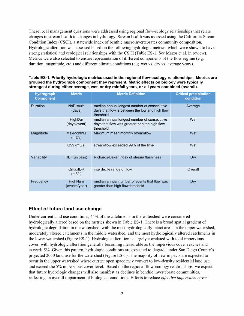
These local management questions were addressed using regional flow-ecology relationships that relate changes in stream health to changes in hydrology. Stream health was assessed using the California Stream Condition Index (CSCI), a statewide index of benthic macroinvertebrates community composition. Hydrologic alteration was assessed based on the following hydrologic metrics, which were shown to have strong statistical and ecological relationships with the CSCI (Table ES-1; See Mazor et al. in review). Metrics were also selected to ensure representation of different components of the flow regime (e.g. duration, magnitude, etc.) and different climate conditions (e.g. wet vs. dry vs. average years).

Table ES-1. Priority hydrologic metrics used in the regional flow-ecology relationships. Metrics are grouped the hydrograph component they represent. Metric effects on biology were typically strongest during either average, wet, or dry rainfall years, or all years combined (overall).

Hydrograph Component

Metric Metric Definition Critical precipitation condition

Duration NoDisturb (days)

median annual longest number of consecutive days that flow is between the low and high flow threshold

Average

HighDur (days/event)

median annual longest number of consecutive days that flow was greater than the high flow threshold

Wet

Magnitude MaxMonthQ (m3/s)

Maximum mean monthly streamflow Wet

Q99 (m3/s) streamflow exceeded 99% of the time Wet

Variability RBI (unitless) Richards-Baker index of stream flashiness Dry

QmaxIDR (m3/s)

interdecile range of flow Overall

Frequency HighNum (events/year)

median annual number of events that flow was greater than high flow threshold

Dry

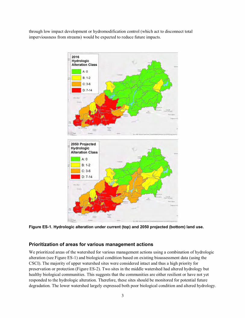
Effect of future land use change Under current land use conditions, 44% of the catchments in the watershed were considered hydrologically altered based on the metrics shown in Table ES-1. There is a broad spatial gradient of hydrologic degradation in the watershed, with the most hydrologically intact areas in the upper watershed, moderately altered catchments in the middle watershed, and the most hydrologically altered catchments in the lower watershed (Figure ES-1). Hydrologic alteration is largely correlated with total impervious cover, with hydrologic alteration generally becoming measurable as the impervious cover reaches and exceeds 5%. Given this pattern, hydrologic conditions are expected to degrade under San Diego County’s projected 2050 land use for the watershed (Figure ES-1). The majority of new impacts are expected to occur in the upper watershed where current open space may convert to low-density residential land use and exceed the 5% impervious cover level. Based on the regional flow-ecology relationships, we expect that future hydrologic changes will also manifest as declines in benthic invertebrate communities, reflecting an overall impairment of biological conditions. Efforts to reduce effective impervious cover

3

through low impact development or hydromodification control (which act to disconnect total imperviousness from streams) would be expected to reduce future impacts.

Figure ES-1. Hydrologic alteration under current (top) and 2050 projected (bottom) land use.

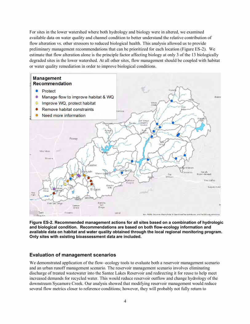
Prioritization of areas for various management actions We prioritized areas of the watershed for various management actions using a combination of hydrologic alteration (see Figure ES-1) and biological condition based on existing bioassessment data (using the CSCI). The majority of upper watershed sites were considered intact and thus a high priority for preservation or protection (Figure ES-2). Two sites in the middle watershed had altered hydrology but healthy biological communities. This suggests that the communities are either resilient or have not yet responded to the hydrologic alteration. Therefore, these sites should be monitored for potential future degradation. The lower watershed largely expressed both poor biological condition and altered hydrology.

4

For sites in the lower watershed where both hydrology and biology were in altered, we examined available data on water quality and channel condition to better understand the relative contribution of flow alteration vs. other stressors to reduced biological health. This analysis allowed us to provide preliminary management recommendations that can be prioritized for each location (Figure ES-2). We estimate that flow alteration alone is the principle factor affecting biology at only 3 of the 13 biologically degraded sites in the lower watershed. At all other sites, flow management should be coupled with habitat or water quality remediation in order to improve biological conditions.

Figure ES-2. Recommended management actions for all sites based on a combination of hydrologic and biological condition. Recommendations are based on both flow-ecology information and available data on habitat and water quality obtained through the local regional monitoring program. Only sites with existing bioassessment data are included.

Evaluation of management scenarios We demonstrated application of the flow–ecology tools to evaluate both a reservoir management scenario and an urban runoff management scenario. The reservoir management scenario involves eliminating discharge of treated wastewater into the Santee Lakes Reservoir and redirecting it for reuse to help meet increased demands for recycled water. This would reduce reservoir outflow and change hydrology of the downstream Sycamore Creek. Our analysis showed that modifying reservoir management would reduce several flow metrics closer to reference conditions; however, they will probably not fully return to

5

reference condition due to the ongoing contribution of urban runoff. Overall, certain components of the hydrograph (usually under high flow conditions) in Sycamore Creek will improve, but is likely to remain in degraded hydrologic and biological condition, even if discharges from Santee Lakes Reservoir are eliminated following the proposed management scenario.

We modeled two urban runoff management scenarios: 1) disconnecting impervious areas from discharging to streams (i.e. reducing impervious cover), and 2) implementing stormwater retention facilities that can capture 85th percentile of a 24-hour rain event. Disconnecting imperviousness decreases the extent of hydrologic alteration in the downstream reaches. However, flow metrics do not return to levels associated with healthy biological communities until the total imperviousness is at or below 5%. Analysis shows that for most metrics, there is a 66% likelihood of meeting flow targets at 5% total impervious cover and an 80% likelihood of meeting flow targets at 2% total impervious cover (i.e. with stormwater control measures installed). The sensitivity of the creek to relatively low levels of impervious cover is consistent with past studies from southern California. In contrast, retention of the 85% storm event (as is currently required through the local stormwater permit) resulted in flow metrics that met all target values.

Utility of the ELOHA approach for establishing flow-ecology relationships A major objective of this case study was to evaluate the ability to apply the flow–ecology relationships derived from the regional ELOHA analysis to inform local watershed-scale decisions. Our results illustrate that several of the stated advantages of the ELOHA approach do aid in such watershed-scale application. The ability to apply regionally derived flow targets to inform local decisions is a major advantage of the ELOHA approach. This eliminates the need to develop local flow–ecology relationships for every stream of interest, as is the case in more traditional instream flow methods. The tools developed through the regional analysis provided readily transferable tools for local stakeholders to produce measures of hydrologic change for any location of interest and to explore how those values would change under different land-use or management scenarios. This had the dual benefit of allowing for robust analysis and providing a vehicle for stakeholder engagement in setting management priorities related to instream flow. Ultimate policy decisions about how streams are managed must balance many competing needs. This case study shows how regional flow-ecology relationships can help inform these decisions.

Lessons learned for future implementation of regional flow-ecology relationships Future efforts can build on the experiences from this case study and continue to refine an iterative process of developing flow targets that are scientifically defensible, practical (i.e., can lead to management actions), and consistent with local stakeholder needs. Key lessons learned from this effort include:

1. Include a broad set of engaged stakeholders, including regulatory agencies, municipalities, water agencies, non-governmental organizations, and researchers. This ensures a broad perspective in the deliberations and increases the likelihood of developing balanced recommendations.

2. Invest in educating the stakeholders early in the process on the underlying science and the rationale behind how regional flow targets were developed. This promotes engagement and fosters creative solutions to the complex challenges of flow management.

3. Invest the time to compile high quality local data sources and show how local data can be used in the evaluation process. Identify the areas were future date collection can most improve outputs of the flow–ecology analysis (e.g., local rainfall data, more refined land use, water quality data). This can inform future monitoring.

4. Develop documentation that clearly illustrates how the products of the flow–ecology analysis can be used in the context of existing regulatory or management programs.

6

The San Diego River implementation case study also produced several technical recommendations that can improve our ability to apply flow-ecology relationships to manage southern California streams:

1. Several flow metrics, particularly those associated with flow duration, may require modification for use in streams where the natural condition is intermittent or ephemeral. Natural intermittency poses fewer issues when developing regional flow-ecology relationships based on hundreds of sites. However, application of the resultant thresholds to specific streams that may have been naturally intermittent can lead to erroneous results.

2. Metrics associated with flow durations should be calculated on a single threshold value based on reference conditions. Estimating hydrologic change based on a moving threshold estimated separately for current and reference conditions may produce erroneous results.

3. Need to improve the representation of the drainage system to provide a more accurate hydrologic foundation for analysis. This would ultimately include improved mapping of discharges, diversions, stormwater control facilities, LID, etc. for incorporation into modeling scenarios and effects.

4. Consider expanding the analysis to include additional elements in future case studies a. Include other stream or water body types b. Include other indicators (e.g. algae) c. Explore how consistent/transferable findings are from one watershed to another d. Explore application in watersheds that cross jurisdictional boundaries

7

INTRODUCTION Flow regime has been shown to affect a broad suite of ecological processes and biological communities (Bunn and Arthington 2002, Naiman et al. 2002, Poff et al. 1997, Poff and Zimmerman 2010, Novak et al. 2015). Many studies have demonstrated that alterations of flow regime can be associated with changes in macroinvertebrate assemblages, which are used as key bioindicators for many regulatory and management programs globally (Pringle et al. 2000, Miller et al. 2007, DeGasperi et al. 2009, Poff & Zimmerman 2010). Although a basic understanding of the relationship between flow alteration and ecological response exists (Poff et al. 2010), few studies have demonstrated how to develop regulatory or management objectives (or targets) based on these relationships. Establishing quantitative and predictive relationships between change in flow and change in biological community composition is a critical step in using bioassessment indicators to establish measures of project performance or regulatory compliance.

Various approaches have been used to develop relationships between flow characteristics and biological response. Examples include use of habitat suitability models that relate flow change to requisite habitats for target taxa (e.g., MesoHABSIM, Parasiewicz 2009; and PHABSIM, Beecher et al. 2010); establishment of functional flow regimes to support species of management concern (McClain et al. 2014, Yarnell et al. 2015); and use of statistical ranges of sustainability based on unaltered hydrographs (Richter et al. 2011). Concepts from several of these approaches have been organized into the Ecological Limits of Hydrologic Alteration (ELOHA) framework (Poff et al. 2010). The ELOHA framework uses a variety of hydrologic and biologic tools to determine and implement environmental flows at the regional scale. Results of the ELOHA analysis can inform management decisions, such as release rates from dams, reservoirs or basins, diversion volumes for irrigation or water re-use, or flows associated with stream restoration. Because the ELOHA framework provides a way to assess the effect of flow alteration on the condition of biological communities (vs. individual taxa) on a regional basis, it is a useful approach for setting targets across a wide range of geographies and stream types where comprehensive detailed site-specific investigations are not practical. The ELOHA framework includes elements of stream classification, estimation of flow alternation (termed “delta H”) and development of flow ecology relationships based on the relationship between delta H and changes in the biological community (“delta B”).

There have been several recent applications of the ELOHA framework to develop flow targets for benthic invertebrates, fish, mussels, amphibians, and aquatic and riparian vegetation. Buchanan et al. (2013) completed the ELOHA approach in the mid-Atlantic region of the U.S. and was able to show clear relationships between changes in a subset of six flow metrics and six benthic invertebrate endpoints. This allowed the authors to recommend specific metrics that could be used for monitoring and assessment. McManamay et al (2013) applied ELOHA through a case study in North Carolina to assess the effect of a stream restoration on fish and riparian communities. Although the ELOHA framework worked well at documenting effects of the restoration projects, confounding factors (e.g., associations between delta H and water chemistry alteration) produced equivocal relationships between flow alteration and response of the fish community. The Nature Conservancy has developed ecosystem flow recommendations for the Susquehanna River Basin (DePhilip and Moberg 2010) and the upper Ohio River Basin (DePhilip and Moberg 2013) that provide seasonally differentiated targets for different stream classes and multiple biological endpoints (e.g., fish, mussels, amphibians, vegetation). Solans and Jalon (2016) used a series of flow alteration-ecological response curves to develop environmental flow standards for the Ebro River Basin in the Iberian Peninsula. Most recently, Mazor et al. (in review) capitalized on extensive regional biomonitoring data and a set of regional hydrologic models developed by Sengupta et al. (in review) to develop flow-ecology relationships for southern California based on benthic macroinvertebrate communities as a measure of stream health.

Previous studies have demonstrated the utility of the ELOHA framework for establishing flow targets and thresholds using relationships between changes in flow and changes in biological condition. Broad scale

8

application of ecologically derived flow targets (or thresholds) can be informed by case studies that demonstrate how flow-ecology relationships can be used to inform actual management decisions. In addition to the study by McManamay et al (2013), the main place where flow-targets have been implemented to inform management actions is in the Juanita Creek Watershed in Washington State, USA (King County 2012). The Juanita Creek study evaluated the effectiveness of seven potential stormwater mitigation scenarios at achieving biologically relevant flow targets using a calibrated Hydrological Simulation Program-Fortran (HSPF) model; a single scenario was identified which would accomplish the stated watershed goals. To our knowledge, none of the previous cases studies attempted to apply regionally-derived flow-ecology relationships (such as those developed for Southern California) to inform decisions at the watershed scale. Additional case studies that demonstrate this application can provide a template for future applications of flow-ecology based targets, and allow for consideration of lessons learned to refine these future applications. Such case studies are also important because they provide an opportunity to work with local watershed stakeholders to identify management needs and apply ecohydrology analysis to inform decisions in a way that balances consideration of ecological endpoints with other needs (e.g., water supply management, new infrastructure and development, flood control).

The goal of this project is to demonstrate how the regionally derived flow–ecology relationships developed by Mazor et al. (in review) can be implemented at a watershed scale to guide management targets/decisions. Regional relationships allow us to describe general patterns of response in biological communities to changes in hydrology. Local case studies are critical to determine how these relationships can be applied to site-specific decisions, and to identify areas where the regional relationships may need to be refined to better support local application.

9

METHODS

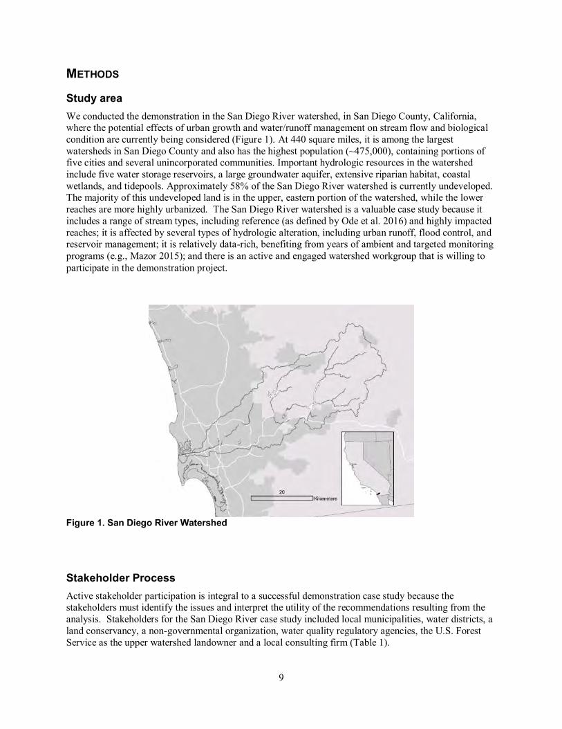
Study area We conducted the demonstration in the San Diego River watershed, in San Diego County, California, where the potential effects of urban growth and water/runoff management on stream flow and biological condition are currently being considered (Figure 1). At 440 square miles, it is among the largest watersheds in San Diego County and also has the highest population (~475,000), containing portions of five cities and several unincorporated communities. Important hydrologic resources in the watershed include five water storage reservoirs, a large groundwater aquifer, extensive riparian habitat, coastal wetlands, and tidepools. Approximately 58% of the San Diego River watershed is currently undeveloped. The majority of this undeveloped land is in the upper, eastern portion of the watershed, while the lower reaches are more highly urbanized. The San Diego River watershed is a valuable case study because it includes a range of stream types, including reference (as defined by Ode et al. 2016) and highly impacted reaches; it is affected by several types of hydrologic alteration, including urban runoff, flood control, and reservoir management; it is relatively data-rich, benefiting from years of ambient and targeted monitoring programs (e.g., Mazor 2015); and there is an active and engaged watershed workgroup that is willing to participate in the demonstration project.

Figure 1. San Diego River Watershed

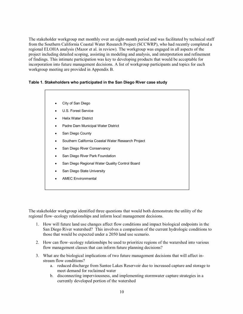
Stakeholder Process Active stakeholder participation is integral to a successful demonstration case study because the stakeholders must identify the issues and interpret the utility of the recommendations resulting from the analysis. Stakeholders for the San Diego River case study included local municipalities, water districts, a land conservancy, a non-governmental organization, water quality regulatory agencies, the U.S. Forest Service as the upper watershed landowner and a local consulting firm (Table 1).

10

The stakeholder workgroup met monthly over an eight-month period and was facilitated by technical staff from the Southern California Coastal Water Research Project (SCCWRP), who had recently completed a regional ELOHA analysis (Mazor et al. in review). The workgroup was engaged in all aspects of the project including detailed scoping, assisting in modeling and analysis, and interpretation and refinement of findings. This intimate participation was key to developing products that would be acceptable for incorporation into future management decisions. A list of workgroup participants and topics for each workgroup meeting are provided in Appendix B.

Table 1. Stakeholders who participated in the San Diego River case study

The stakeholder workgroup identified three questions that would both demonstrate the utility of the regional flow–ecology relationships and inform local management decisions.

1. How will future land use changes affect flow conditions and impact biological endpoints in the San Diego River watershed? This involves a comparison of the current hydrologic conditions to those that would be expected under a 2050 land use scenario.

2. How can flow–ecology relationships be used to prioritize regions of the watershed into various flow management classes that can inform future planning decisions?

3. What are the biological implications of two future management decisions that will affect in-stream flow conditions?

a. reduced discharge from Santee Lakes Reservoir due to increased capture and storage to meet demand for reclaimed water

b. disconnecting imperviousness, and implementing stormwater capture strategies in a currently developed portion of the watershed

City of San Diego

U.S. Forest Service

Helix Water District

Padre Dam Municipal Water District

San Diego County

Southern California Coastal Water Research Project

San Diego River Conservancy

San Diego River Park Foundation

San Diego Regional Water Quality Control Board

San Diego State University

AMEC Environmental

11

Regional ELOHA (flow-ecology) analysis The local management questions were addressed using regional flow-ecology relationships conducted for southern California that relates changes in stream health to changes in hydrology. Stream health was assessed using the California Stream Condition Index (CSCI), a statewide index of benthic macroinvertebrates community composition. Hydrologic alteration was assessed based on a series of hydrologic metrics, which were shown to have strong statistical and ecological relationships with the CSCI (Mazor et al. in review). Metrics were also selected to ensure representation of different components of the flow regime (e.g. duration, magnitude, etc.) and different climate conditions (e.g. wet vs. dry vs. average years). Because we lack measured flow data for both current and historic conditions at most bioassessment sites, both were estimated using watershed models.

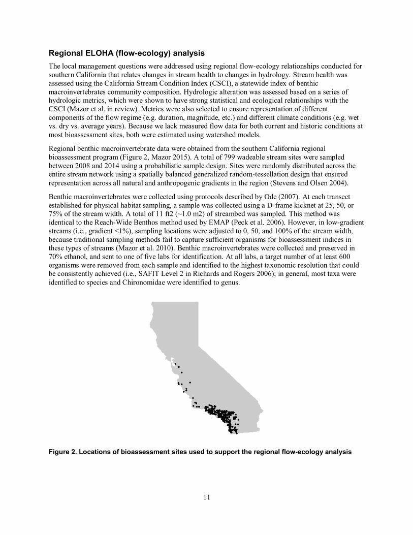
Regional benthic macroinvertebrate data were obtained from the southern California regional bioassessment program (Figure 2, Mazor 2015). A total of 799 wadeable stream sites were sampled between 2008 and 2014 using a probabilistic sample design. Sites were randomly distributed across the entire stream network using a spatially balanced generalized random-tessellation design that ensured representation across all natural and anthropogenic gradients in the region (Stevens and Olsen 2004).

Benthic macroinvertebrates were collected using protocols described by Ode (2007). At each transect established for physical habitat sampling, a sample was collected using a D-frame kicknet at 25, 50, or 75% of the stream width. A total of 11 ft2 (~1.0 m2) of streambed was sampled. This method was identical to the Reach-Wide Benthos method used by EMAP (Peck et al. 2006). However, in low-gradient streams (i.e., gradient <1%), sampling locations were adjusted to 0, 50, and 100% of the stream width, because traditional sampling methods fail to capture sufficient organisms for bioassessment indices in these types of streams (Mazor et al. 2010). Benthic macroinvertebrates were collected and preserved in 70% ethanol, and sent to one of five labs for identification. At all labs, a target number of at least 600 organisms were removed from each sample and identified to the highest taxonomic resolution that could be consistently achieved (i.e., SAFIT Level 2 in Richards and Rogers 2006); in general, most taxa were identified to species and Chironomidae were identified to genus.

Figure 2. Locations of bioassessment sites used to support the regional flow-ecology analysis

12

Benthic macroinvertebrate data was used to calculate the California Stream Condition Index (CSCI; Mazor et al. 2016). The CSCI is a predictive index that compares observed taxa and metrics to values expected under reference conditions based on site-specific landscape-scale environmental variables, such as watershed area, geology, and climate. It includes two components: a ratio of observed-to-expected taxa (O/E) and a predictive multi-metric index (MMI) made up of 6 metrics related to ecological structure and function of the benthic macroinvertebrate assemblage. Because the CSCI and all of its components are based on site-specific reference expectations, scores are minimally influenced by major natural gradients. Therefore, CSCI scores, by definition, compare existing to reference conditions and can be used as a measure of biological alteration (delta B) under anthropogenic stress. CSCI scores and all components were classified as indicating “intact” or “altered” condition, using the normal approximation of the 10th percentile of CSCI reference calibration scores as a threshold (Mazor et al. 2016). For the CSCI, this equates to a score of 0.79 (where 1 is the reference expectation) as the threshold between biologically intact and altered.

Hydrologic alteration was modeled at 584 of the 799 bioassessment sites using HEC-HMS (ACOE 2000). The remaining 215 bioassessment sites were dropped from the analysis because the rainfall data at those locations was insufficient or did not meet quality control criteria for use in model development. Past studies have assessed hydrologic alteration based on empirical observations, often using a space for time substitution (i.e. comparing distinct hydrologically intact vs. altered locations instead of comparing hydrologic change over time). Modeling provides a mechanism to estimate hydrologic alteration at any location where biological data is available, thereby allowing larger data sets to be included in flow-ecology analysis (DeGasperi et al. 2009). Given the size of the southern California data set (584 sites), there was a need to balance the desire to model hydrologic alteration with the practical considerations of needing a tool that could be readily applied to a high number of sites (Sengupta et al. in review). HEC-HMS provides the ability to produce a continuous time series of estimated flow through parameterization of relatively small number of variables in the model (HEC-HMS manual version 4.1, Xuefeng and Steinman 2009).

A set of 26 HEC-HMS models was developed as part of the regional flow-ecology analysis to represent the range of watershed conditions present in the region. Therefore, one of the 26 models can be applied to produce a daily flow time series for every bioassessment site based on basin properties draining to that site. This obviates the need to develop a unique model for every site. Inputs used to develop and parameterize the models are grouped in three categories (Table 2): 1) watershed-specific data (e.g., area, and imperviousness), 2) site-specific data (e.g., observed flow, precipitation) and 3) model-specific parameters (e.g., initial loss, number of reservoirs).

13

Table 2. Parameters used to develop HEC-HMS models for application to the regional bioassessment sampling sites. Parameters in bold were adjusted during simulation of natural conditions at each site.

HEC-HMS Method Parameters

Watershed Specific

Area

Imperviousness

Time of concentration

Site Specific

Observed flow

Observed precipitation

Model Specific

Simple Canopy Maximum Storage (in)

Initial Storage (%)

Simple Surface Maximum Storage (in)

Initial Storage (%)

Deficit and Constant (Loss)

Initial Deficit (in)

Maximum Deficit (in)

Constant Rate (in/hr)

Clark Unit Hydrograph (Transform)

Time of Concentration (hr)

Storage Coefficient (hr)

Linear Reservoir (Baseflow)

Ground Water (GW) 1 Initial Discharge (cfs)

GW 1 Storage Coefficient (hr)

# of GW 1 Reservoirs

GW 2 Initial Discharge (cfs)

GW 2 Storage Coefficient (in)

# of GW 2 Reservoirs

Each model was sequentially calibrated for four criteria: visual hydrograph match, Nash-Sutcliffe efficiency (NSE), percent low flow days, and Richard-Baker Index of flashiness. These calibration endpoints were selected based on relevance for supporting the instream biological communities (Konrad and Booth 2005, Morley and Karr 2002). Calibrating to all four measures produced models tuned to simulate flow conditions relevant for supporting in-stream biological communities. Models were calibrated for a 3-year period and were then validated for temporal and spatial performance. For temporal validation, the calibrated models were run for years outside of the calibration period and matched with the observed flow data. In all cases, model performance (as measured by NSE) during the validation period was within 15% of performance during the calibration period.

To evaluate spatial performance, we applied statistical ‘jackknifing’ to all calibrated gages. In this analysis, each modeled gage is treated as an ‘ungaged’ site, and the remaining 25 models are used to predict flows at that site. The models were fitted to the ‘ungaged’ site by inputting watershed-specific data and model-specific parameters, but without changes to the model-specific parameters. These simulations were run for the 3-year calibration period. Approximately 75% of the sites had an acceptable NSE value higher than 0.5 (Moriasi et al. 2007). A final validation was performed by comparing modeled output to measured flow at 16 bioassessment sites with nearby flow gages (but not included in the model development). At 11 of the sites, the R2 values averaged 0.61; the range varied from 0.20 to 0.95. Further details on the model validation are found in Sengupta et al. (in review).

14

One of the 26 validated models was assigned to each of 584 bioassessment sites with adequate rainfall data in the southern California region based on similarity of watershed characteristics that were associated with observed hydrology. The assignment was done with a model-selection tool built by 1) classifying the models into 8 clusters based on observed flow metrics; 2) creating a random forest model to predict cluster membership based on watershed characteristics (i.e., elevation maximum and range, mean annual temperature, watershed area, mean catchment-wide summer precipitation, and soil erodibility factor); and 3) calculating proximity values (i.e., the frequency that a site and a model are predicted to be in the same cluster) between novel sites and each of the 26 models. For each bioassessment site, the model with the highest proximity value was selected for further analysis. Details about the development of the model-selection tool, and its performance, are provided in Sengupta et al. (in review).

The watershed models were used to produce an hourly time series of flow for a period of 23 years (1990 -2013) for the 584 bioassessment sites. A subset of 6 years was selected for each site to calculate specific flow metrics. The six years were chosen to include two wet, two dry, and two average rainfall years based on long-term climate records. The six years were also selected based on the availability of high quality, complete rainfall records (i.e. no missing values or apparent anomalies). A challenge of the ELOHA approach is the need to compare current hydrologic conditions to reference in order to estimate hydrologic change (delta H). Because we seldom have data on historical flows, we rely on modeling to estimate reference conditions. Hourly hydrographs were estimated for both current and reference conditions at each site following Sengupta et al. (in review). Hourly hydrographs were aggregated to daily discharge, and a suite of flow metrics that represent different aspects of flow were calculated for both current and reference conditions (Table 3) Metrics were calculated for wet, dry, and average precipitation conditions, as well as for all 6 years combined. Metric-precipitation combinations that validated poorly (i.e., r2 < 0.25) with observed flow were excluded from further analysis. This resulted in a total of 116 metric–precipitation combinations for analysis. For each metric–precipitation combination, hydrologic alteration (delta H) was characterized as differences between simulated current and reference conditions. “Reference condition” was estimated by adjusting model parameters to reflect undeveloped watershed conditions. Delta H for magnitude metrics was normalized by reference condition or 0.0283 cms (whichever was larger) to account for the effect of catchment size on discharge magnitude. Details on the hydrological analysis and modeling approach can be found in Appendix A.

15

Table 3. Flow metrics sorted by metric type and period of evaluation. O=overall, W=wet years, A= average years, D=dry years. Unless otherwise noted, metrics are from Konrad et al. (2008), Konrad, personal communication, Colwell (1974), or Bledsoe (personal communication).

Metric Description O W A D Duration

LowDur days/event Median annual longest number of consecutive days that flow was less than or equal to the low flow threshold

• • •

HighDur days/event Median annual longest number of consecutive days that flow was greater than the high flow threshold

• •

NoDisturb days/year Median annual longest number of consecutive days that flow between the low and high flow threshold

• • • •

Hydroperiod proportion Fraction of period of analysis with flows • • •

Per_LowFlow proportion Percent of time with flow below 0.0283 cms • • • •

Frequency

HighNum events/year

Median annual number of events that flow was greater than high flow threshold, an event is a continuous period when daily flow exceeds the threshold

• • • •

FracYearsNoFlow proportion Fraction of years with at least one no-flow day •

MedianNoFlowDays days/year Median annual number of no-flow days • • • • Magnitude MaxMonthQ cms Maximum mean monthly streamflow • • • • MinMonthQ cms Minimum mean monthly streamflow • • • • Q01 cms 1st percentile of daily streamflow • • • • Q05 cms 5th percentile of daily streamflow • • • • Q10 cms 10th percentile of daily streamflow • • • • Q25 cms 25th precentile of daily streamflow • • • • Q50 cms 50th percentile of daily streamflow • • • • Q75 cms 75th precentile of daily streamflow • • • • Q90 cms 90th precentile of daily streamflow • • • • Q95 cms 95th percentile of daily streamflow • • • • Q99 cms 99th percentile of daily streamflow • • • •

Qmax cms Median annual maximum daily streamflow • • • •

Qmean cms Mean streamflow for the period of analysis • • • •

QmeanMEDIAN cms Median annual mean streamflow • • • • Qmed cms Median daily streamflow • • • • Qmin cms Median annual minimum daily streamflow • • • • Timing

C_C ratio Colwell's constancy (C) a measure of flow uniformity. • • • •

C_CP ratio Colwell's maximized constancy (C/P). Likelihood that flow is constant through the year

• • • •

16

17

Metric Duration

C_M ratio Colwell's contingency (M). Repeatability of seasonal patterns. • • • •

C_MP ratio Colwell's maximized contingency (M/P). Likelihood that the pattern of high and low flow events is repeated across years.

• • • •

C_P ratio Colwell's predictability (P=C+M). Likelihood of being able to predict high and low flow events • • • •

MinMonth month Month of minimum mean monthly streamflow • •

MaxMonth month Month of maximum mean monthly streamflow •

Variability

RBI Unitless Richard Baker Index (flashiness) • • •

SFR proportion 90th percentile of percent daily change in streamflow on days when streamflow is receding (storm-flow recession) •

QminIDR cms Interdecile range of annual minima •

QmeanIDR cms Interdecile range of annual means •

QmaxIDR cms Interdecile range of annual maxima •

Hydrologic thresholds that result in biological response were evaluated for each flow metric-precipitation condition combination, based on nine biological response variables (i.e. the CSCI and its component metrics). Hydrologic metrics were evaluated for overall climatic conditions, as well as for wet, dry, or average precipitation years. The 116 metric-precipitation condition combinations were used to predict each of the nine biological response variables in boosted regression tree models using the gbm package in R (Ridgeway 2015, R Core Team 2016), and the importance of each predictor was ranked (Friedman 2001). Ranks were averaged across all models, and the best ranked precipitation condition within each metric was selected for further analysis. Ecologically derived targets were then established for each flow metric. Further detail about modeling biological responses to hydrologic alteration can be found in Mazor et al. (in review).

In order to set targets for hydrologic metrics based on biological response, we developed logistic regression models of the probability of healthy biological condition as a function of different levels of hydrologic alteration. Targets were set at the level of hydrologic alteration where the probability of healthy biological condition was 50% of the probability at hydrologically unaltered sites. It is important to note that these targets do not represent reference conditions. Increasing and decreasing gradients of hydrologic alteration were analyzed independently against each biological response variable. Across all biological response variables, the most conservative target was selected for further analysis. Logistic regression models were created using the glm function in R with a binomial error distribution and a logit link function (R Core Team, 2016). Metrics were scored 0 if they met targets, 1 if they failed targets, and 2 if they failed targets by more than twice the target value (Figure 3).

18

Figure 3. Example scale for assigning hydrologic alteration scores

An objective of the regional flow-ecology analysis was to identify a subset of priority flow metrics that can be used to inform management actions. Metrics were prioritized based on the following criteria (Mazor et al. in review):

Differentiate hydrologic condition at reference sites vs. altered sites

Have the strongest relationship to biological condition based on boosted regression tree analysis and can produce a hypothesized ecological response

Can be modeled under both current and reference conditions with a high level of confidence

Are amenable to management actions and are expected to respond in predictable ways to deliberate changes in flow conditions

Have minimal redundancy with other metrics; the goal is to select metrics that represent different components of the hydrograph (e.g. magnitude vs. duration)

Based on these criteria and the logistic regression analysis described above, Mazor et al. (in review) identified seven priority flow metrics and associated thresholds of biological response (Table 4). The importance of the seven priority flow metrics varied by climatic condition, with some metrics only being important during certain precipitation conditions (Table 4). Using a subset of metrics has the advantage of allowing management actions to focus on controlling a reasonable set of flow properties that will have the greatest biological effects, as opposed to trying to manage for all 116 metric-precipitation combinations.

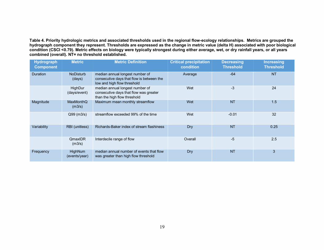
19

Table 4. Priority hydrologic metrics and associated thresholds used in the regional flow-ecology relationships. Metrics are grouped the hydrograph component they represent. Thresholds are expressed as the change in metric value (delta H) associated with poor biological condition (CSCI <0.79). Metric effects on biology were typically strongest during either average, wet, or dry rainfall years, or all years combined (overall). NT= no threshold established.

Hydrograph Component

Metric Metric Definition Critical precipitation condition

Decreasing Threshold

Increasing Threshold

Duration NoDisturb (days)

median annual longest number of consecutive days that flow is between the low and high flow threshold

Average -64 NT

HighDur (days/event)

median annual longest number of consecutive days that flow was greater than the high flow threshold

Wet -3 24

Magnitude MaxMonthQ (m3/s)

Maximum mean monthly streamflow Wet NT 1.5

Q99 (m3/s) streamflow exceeded 99% of the time Wet -0.01 32

Variability RBI (unitless) Richards-Baker index of stream flashiness Dry NT 0.25

QmaxIDR (m3/s)

Interdecile range of flow Overall -5 2.5

Frequency HighNum (events/year)

median annual number of events that flow was greater than high flow threshold

Dry NT 3

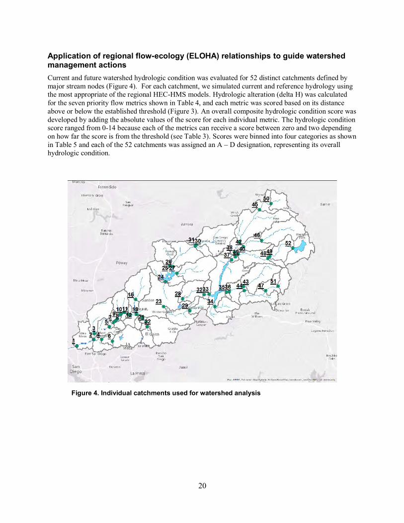
20

Application of regional flow-ecology (ELOHA) relationships to guide watershed management actions Current and future watershed hydrologic condition was evaluated for 52 distinct catchments defined by major stream nodes (Figure 4). For each catchment, we simulated current and reference hydrology using the most appropriate of the regional HEC-HMS models. Hydrologic alteration (delta H) was calculated for the seven priority flow metrics shown in Table 4, and each metric was scored based on its distance above or below the established threshold (Figure 3). An overall composite hydrologic condition score was developed by adding the absolute values of the score for each individual metric. The hydrologic condition score ranged from 0-14 because each of the metrics can receive a score between zero and two depending on how far the score is from the threshold (see Table 3). Scores were binned into four categories as shown in Table 5 and each of the 52 catchments was assigned an A – D designation, representing its overall hydrologic condition.

Figure 4. Individual catchments used for watershed analysis

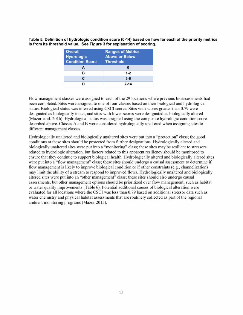
21

Table 5. Definition of hydrologic condition score (0-14) based on how far each of the priority metrics is from its threshold value. See Figure 3 for explanation of scoring.

Overall Hydrologic Condition Score

Ranges of Metrics Above or Below Threshold

A 0 B 1-2 C 3-6 D 7-14

Flow management classes were assigned to each of the 29 locations where previous bioassessments had been completed. Sites were assigned to one of four classes based on their biological and hydrological status. Biological status was inferred using CSCI scores: Sites with scores greater than 0.79 were designated as biologically intact, and sites with lower scores were designated as biologically altered (Mazor et al. 2016). Hydrological status was assigned using the composite hydrologic condition score described above. Classes A and B were considered hydrologically unaltered when assigning sites to different management classes.

Hydrologically unaltered and biologically unaltered sites were put into a “protection” class; the good conditions at these sites should be protected from further designations. Hydrologically altered and biologically unaltered sites were put into a “monitoring” class; these sites may be resilient to stressors related to hydrologic alteration, but factors related to this apparent resiliency should be monitored to ensure that they continue to support biological health. Hydrologically altered and biologically altered sites were put into a “flow management” class; these sites should undergo a causal assessment to determine if flow management is likely to improve biological condition or if other constraints (e.g., channelization) may limit the ability of a stream to respond to improved flows. Hydrologically unaltered and biologically altered sites were put into an “other management” class; these sites should also undergo causal assessments, but other management options should be prioritized over flow management, such as habitat or water quality improvements (Table 6). Potential additional causes of biological alteration were evaluated for all locations where the CSCI was less than 0.79 based on additional stressor data such as water chemistry and physical habitat assessments that are routinely collected as part of the regional ambient monitoring programs (Mazor 2015).

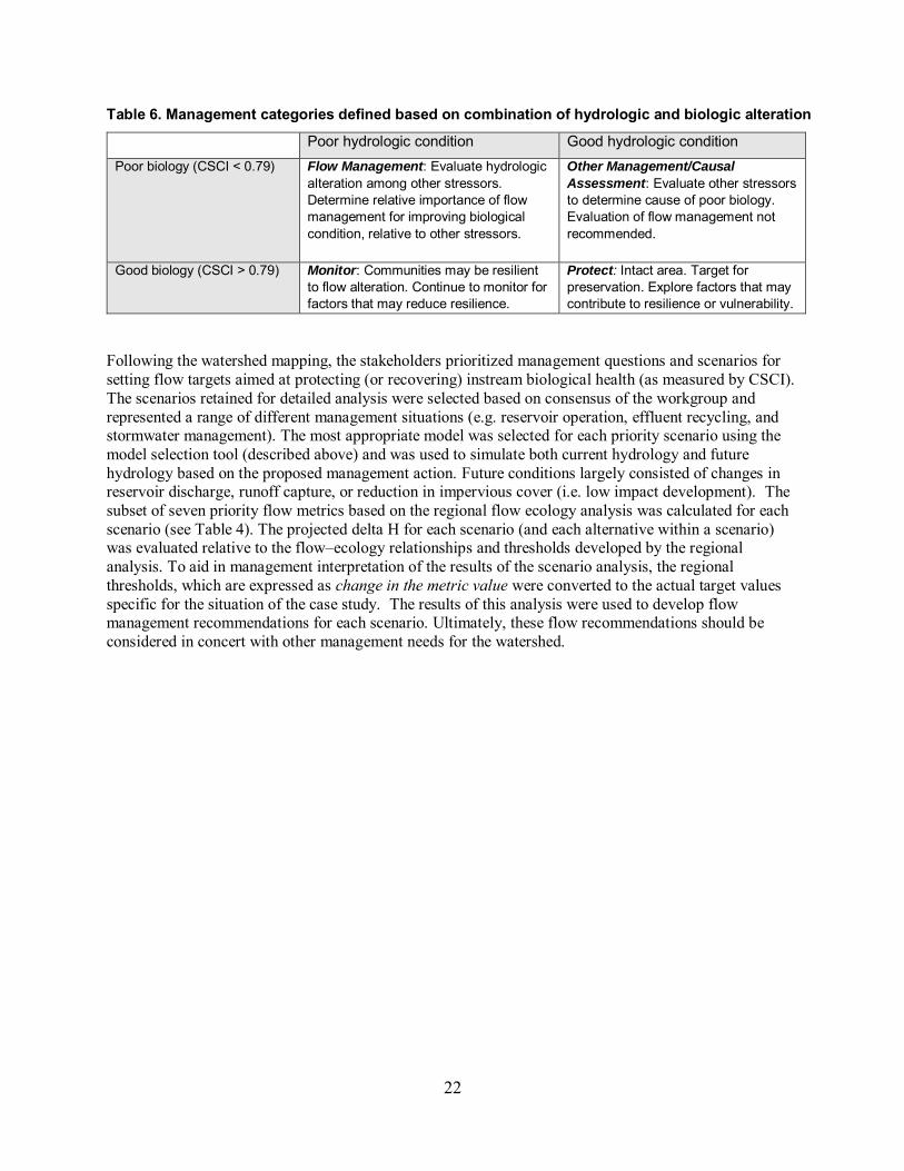
22

Table 6. Management categories defined based on combination of hydrologic and biologic alteration

Poor hydrologic condition Good hydrologic condition Poor biology (CSCI < 0.79) Flow Management: Evaluate hydrologic

alteration among other stressors. Determine relative importance of flow management for improving biological condition, relative to other stressors.

Other Management/Causal

Assessment: Evaluate other stressors to determine cause of poor biology. Evaluation of flow management not recommended.

Good biology (CSCI > 0.79) Monitor: Communities may be resilient to flow alteration. Continue to monitor for factors that may reduce resilience.

Protect: Intact area. Target for preservation. Explore factors that may contribute to resilience or vulnerability.

Following the watershed mapping, the stakeholders prioritized management questions and scenarios for setting flow targets aimed at protecting (or recovering) instream biological health (as measured by CSCI). The scenarios retained for detailed analysis were selected based on consensus of the workgroup and represented a range of different management situations (e.g. reservoir operation, effluent recycling, and stormwater management). The most appropriate model was selected for each priority scenario using the model selection tool (described above) and was used to simulate both current hydrology and future hydrology based on the proposed management action. Future conditions largely consisted of changes in reservoir discharge, runoff capture, or reduction in impervious cover (i.e. low impact development). The subset of seven priority flow metrics based on the regional flow ecology analysis was calculated for each scenario (see Table 4). The projected delta H for each scenario (and each alternative within a scenario) was evaluated relative to the flow–ecology relationships and thresholds developed by the regional analysis. To aid in management interpretation of the results of the scenario analysis, the regional thresholds, which are expressed as change in the metric value were converted to the actual target values specific for the situation of the case study. The results of this analysis were used to develop flow management recommendations for each scenario. Ultimately, these flow recommendations should be considered in concert with other management needs for the watershed.

23

RESULTS AND DISCUSSION

Effect of future land-use change on hydrologic condition To address the question, “how will future land-use changes affect flow conditions and impact biological endpoints in the San Diego River watershed?” we compared the current overall hydrologic condition to the expected future condition based on 2050 SanGIS land-use projections, assuming no installation of stormwater control device or low impact development features.

Under current conditions, 17 of the 52 catchments (33%) scored in the worst two categories of hydrologic alteration, while 35 of 52 (67%) scored in the least hydrologically altered category (Table 7). There appears to be a spatial gradient of hydrologic condition in the watershed, with the most hydrologically intact areas are in the upper watershed, where much of the land is in public ownership and/or there is currently little urban development. Catchments in the poorest hydrologic condition are concentrated in the lower watershed where most of the current development exists. These areas are also downstream of all the reservoirs in the watershed (Figure 5).

Table 7. Distribution of hydrologic alteration scores under current conditions (“A” is least altered, “D” is most altered).

Category # of catchments

Proportion of

catchments A 25 48%

B 10 19%

C 6 12%

D 11 21%

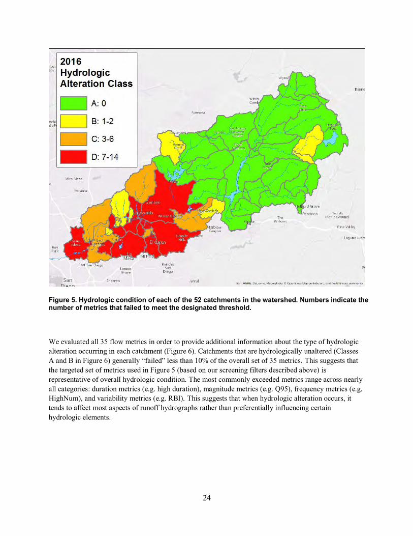
24

Figure 5. Hydrologic condition of each of the 52 catchments in the watershed. Numbers indicate the number of metrics that failed to meet the designated threshold.

We evaluated all 35 flow metrics in order to provide additional information about the type of hydrologic alteration occurring in each catchment (Figure 6). Catchments that are hydrologically unaltered (Classes A and B in Figure 6) generally “failed” less than 10% of the overall set of 35 metrics. This suggests that the targeted set of metrics used in Figure 5 (based on our screening filters described above) is representative of overall hydrologic condition. The most commonly exceeded metrics range across nearly all categories: duration metrics (e.g. high duration), magnitude metrics (e.g. Q95), frequency metrics (e.g. HighNum), and variability metrics (e.g. RBI). This suggests that when hydrologic alteration occurs, it tends to affect most aspects of runoff hydrographs rather than preferentially influencing certain hydrologic elements.

25

Figure 6. Heatmap showing hydrologic metric scores for all catchments and all metrics. Catchment numbers/positions on the x-axis are based on the catchment positions shown in Figure 4.

Hydrologic condition was generally related to catchment imperviousness (Figure 7). In most cases, severe hydrologic alteration was associated with total impervious cover greater than 5%. In all cases, hydrologically unaltered catchments (Classes A and B) had less than 5% total impervious cover, often only 1-2%. This is consistent with past studies that have shown hydrologic and geomorphic responses associated with modest increases in total impervious cover (Hawley and Bledsoe 2011, Vietz et al. 2016).

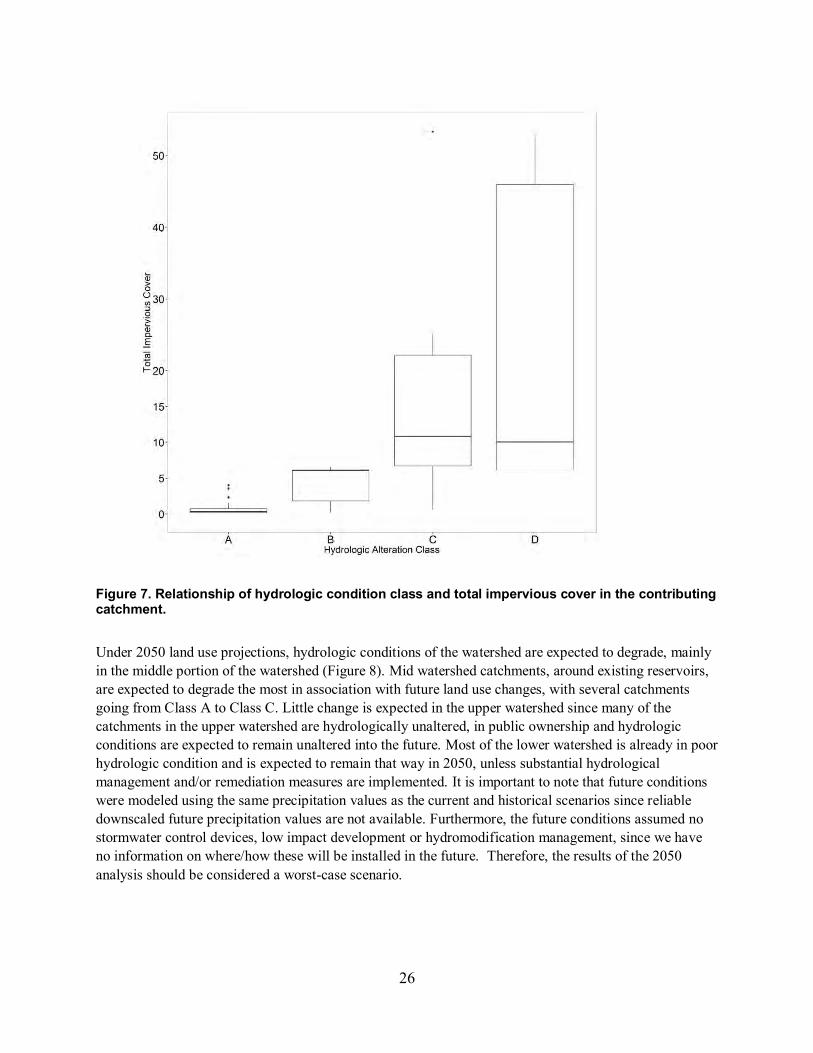
26

Figure 7. Relationship of hydrologic condition class and total impervious cover in the contributing catchment.

Under 2050 land use projections, hydrologic conditions of the watershed are expected to degrade, mainly in the middle portion of the watershed (Figure 8). Mid watershed catchments, around existing reservoirs, are expected to degrade the most in association with future land use changes, with several catchments going from Class A to Class C. Little change is expected in the upper watershed since many of the catchments in the upper watershed are hydrologically unaltered, in public ownership and hydrologic conditions are expected to remain unaltered into the future. Most of the lower watershed is already in poor hydrologic condition and is expected to remain that way in 2050, unless substantial hydrological management and/or remediation measures are implemented. It is important to note that future conditions were modeled using the same precipitation values as the current and historical scenarios since reliable downscaled future precipitation values are not available. Furthermore, the future conditions assumed no stormwater control devices, low impact development or hydromodification management, since we have no information on where/how these will be installed in the future. Therefore, the results of the 2050 analysis should be considered a worst-case scenario.

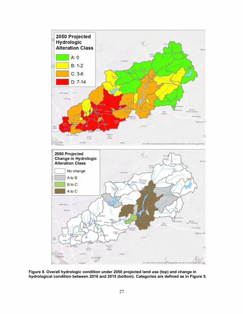
27

Figure 8. Overall hydrologic condition under 2050 projected land use (top) and change in hydrological condition between 2016 and 2015 (bottom). Categories are defined as in Figure 5.

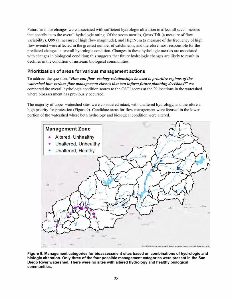
28

Future land use changes were associated with sufficient hydrologic alteration to affect all seven metrics that contribute to the overall hydrologic rating. Of the seven metrics, QmaxIDR (a measure of flow variability), Q99 (a measure of high flow magnitude), and HighNum (a measure of the frequency of high flow events) were affected in the greatest number of catchments, and therefore most responsible for the predicted changes in overall hydrologic condition. Changes in these hydrologic metrics are associated with changes in biological condition; this suggests that future hydrologic changes are likely to result in declines in the condition of instream biological communities.

Prioritization of areas for various management actions To address the question, “How can flow–ecology relationships be used to prioritize regions of the watershed into various flow management classes that can inform future planning decisions?” we compared the overall hydrologic condition scores to the CSCI scores at the 29 locations in the watershed where bioassessment has previously occurred.

The majority of upper watershed sites were considered intact, with unaltered hydrology, and therefore a high priority for protection (Figure 9). Candidate areas for flow management were focused in the lower portion of the watershed where both hydrology and biological condition were altered.

Figure 9. Management categories for bioassessment sites based on combinations of hydrologic and biologic alteration. Only three of the four possible management categories were present in the San Diego River watershed. There were no sites with altered hydrology and healthy biological communities.

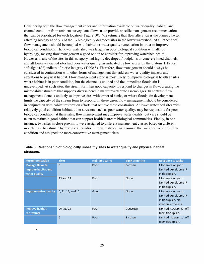
29

Considering both the flow management zones and information available on water quality, habitat, and channel condition from ambient survey data allows us to provide specific management recommendations that can be prioritized for each location (Figure 10). We estimate that flow alteration is the primary factor affecting biology at only 3 of the 13 biologically degraded sites in the lower watershed. At all other sites, flow management should be coupled with habitat or water quality remediation in order to improve biological conditions. The lower watershed was largely in poor biological condition with altered hydrology, making flow management a good option to consider for improving watershed health. However, many of the sites in this category had highly developed floodplains or concrete-lined channels, and all lower watershed sites had poor water quality, as indicated by low scores on the diatom (D18) or soft algae (S2) indices of biotic integrity (Table 8). Therefore, flow management should always be considered in conjunction with other forms of management that address water-quality impacts and alterations to physical habitat. Flow management alone is most likely to improve biological health at sites where habitat is in poor condition, but the channel is unlined and the immediate floodplain is undeveloped. At such sites, the stream form has good capacity to respond to changes in flow, creating the microhabitat structure that supports diverse benthic macroinvertebrate assemblages. In contrast, flow management alone is unlikely to improve sites with armored banks, or where floodplain development limits the capacity of the stream form to respond. In these cases, flow management should be considered in conjunction with habitat restoration efforts that remove these constraints. At lower watershed sites with relatively good condition habitat, other stressors, such as poor water quality, may be responsible for poor biological condition; at these sites, flow management may improve water quality, but care should be taken to maintain good habitat that can support health instream biological communities. Finally, in one instance, two sites in close proximity were assigned to different management classes based on different models used to estimate hydrologic alternation. In this instance, we assumed the two sites were in similar condition and assigned the more conservative management class.

Table 8. Relationship of biologically unhealthy sites to water quality and physical habitat stressors.

.

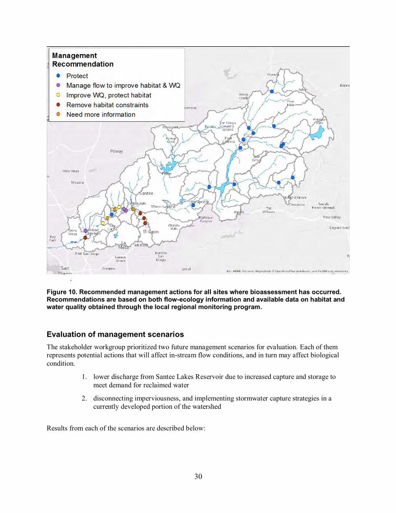
30

.

Figure 10. Recommended management actions for all sites where bioassessment has occurred. Recommendations are based on both flow-ecology information and available data on habitat and water quality obtained through the local regional monitoring program.

Evaluation of management scenarios The stakeholder workgroup prioritized two future management scenarios for evaluation. Each of them represents potential actions that will affect in-stream flow conditions, and in turn may affect biological condition.

1. lower discharge from Santee Lakes Reservoir due to increased capture and storage to meet demand for reclaimed water

2. disconnecting imperviousness, and implementing stormwater capture strategies in a currently developed portion of the watershed

Results from each of the scenarios are described below:

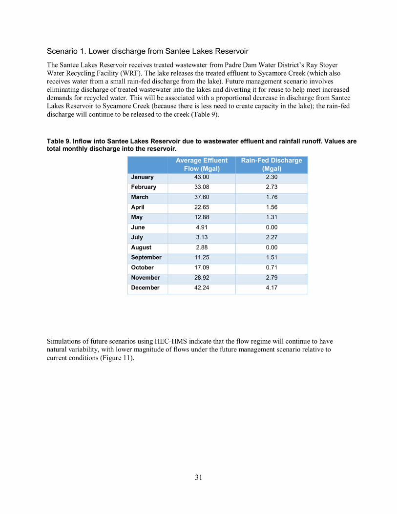
31

Scenario 1. Lower discharge from Santee Lakes Reservoir

The Santee Lakes Reservoir receives treated wastewater from Padre Dam Water District’s Ray Stoyer Water Recycling Facility (WRF). The lake releases the treated effluent to Sycamore Creek (which also receives water from a small rain-fed discharge from the lake). Future management scenario involves eliminating discharge of treated wastewater into the lakes and diverting it for reuse to help meet increased demands for recycled water. This will be associated with a proportional decrease in discharge from Santee Lakes Reservoir to Sycamore Creek (because there is less need to create capacity in the lake); the rain-fed discharge will continue to be released to the creek (Table 9).

Table 9. Inflow into Santee Lakes Reservoir due to wastewater effluent and rainfall runoff. Values are total monthly discharge into the reservoir.

Average Effluent Flow (Mgal)

Rain-Fed Discharge (Mgal)

January 43.00 2.30

February 33.08 2.73

March 37.60 1.76

April 22.65 1.56

May 12.88 1.31

June 4.91 0.00

July 3.13 2.27

August 2.88 0.00

September 11.25 1.51

October 17.09 0.71

November 28.92 2.79

December 42.24 4.17

Simulations of future scenarios using HEC-HMS indicate that the flow regime will continue to have natural variability, with lower magnitude of flows under the future management scenario relative to current conditions (Figure 11).

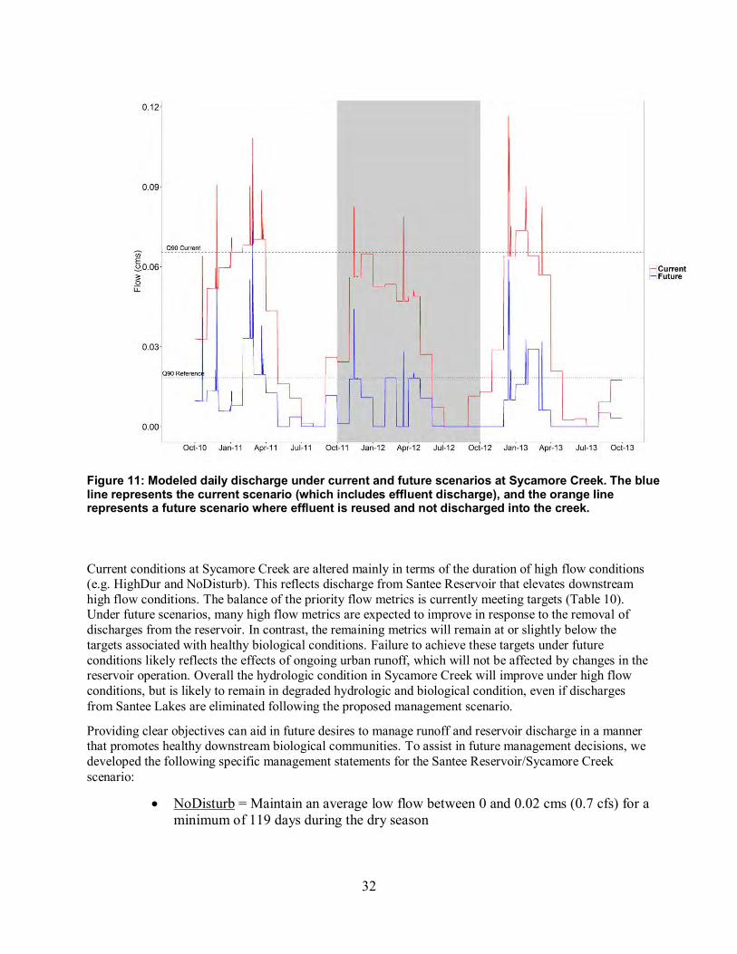
32

Figure 11: Modeled daily discharge under current and future scenarios at Sycamore Creek. The blue line represents the current scenario (which includes effluent discharge), and the orange line represents a future scenario where effluent is reused and not discharged into the creek.

Current conditions at Sycamore Creek are altered mainly in terms of the duration of high flow conditions (e.g. HighDur and NoDisturb). This reflects discharge from Santee Reservoir that elevates downstream high flow conditions. The balance of the priority flow metrics is currently meeting targets (Table 10). Under future scenarios, many high flow metrics are expected to improve in response to the removal of discharges from the reservoir. In contrast, the remaining metrics will remain at or slightly below the targets associated with healthy biological conditions. Failure to achieve these targets under future conditions likely reflects the effects of ongoing urban runoff, which will not be affected by changes in the reservoir operation. Overall the hydrologic condition in Sycamore Creek will improve under high flow conditions, but is likely to remain in degraded hydrologic and biological condition, even if discharges from Santee Lakes are eliminated following the proposed management scenario.

Providing clear objectives can aid in future desires to manage runoff and reservoir discharge in a manner that promotes healthy downstream biological communities. To assist in future management decisions, we developed the following specific management statements for the Santee Reservoir/Sycamore Creek scenario:

NoDisturb = Maintain an average low flow between 0 and 0.02 cms (0.7 cfs) for a minimum of 119 days during the dry season

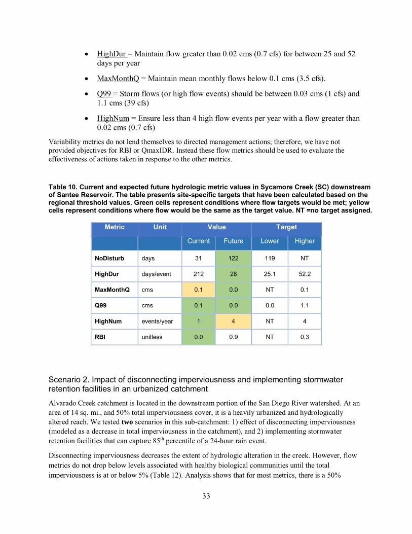
33

HighDur = Maintain flow greater than 0.02 cms (0.7 cfs) for between 25 and 52 days per year

MaxMonthQ = Maintain mean monthly flows below 0.1 cms (3.5 cfs).

Q99 = Storm flows (or high flow events) should be between 0.03 cms (1 cfs) and 1.1 cms (39 cfs)

HighNum = Ensure less than 4 high flow events per year with a flow greater than 0.02 cms (0.7 cfs)

Variability metrics do not lend themselves to directed management actions; therefore, we have not provided objectives for RBI or QmaxIDR. Instead these flow metrics should be used to evaluate the effectiveness of actions taken in response to the other metrics.

Table 10. Current and expected future hydrologic metric values in Sycamore Creek (SC) downstream of Santee Reservoir. The table presents site-specific targets that have been calculated based on the regional threshold values. Green cells represent conditions where flow targets would be met; yellow cells represent conditions where flow would be the same as the target value. NT =no target assigned.

Metric Unit Value Target

Current Future Lower Higher

NoDisturb days 31 122 119 NT

HighDur days/event 212 28 25.1 52.2

MaxMonthQ cms 0.1 0.0 NT 0.1

Q99 cms 0.1 0.0 0.0 1.1

HighNum events/year 1 4 NT 4

RBI unitless 0.0 0.9 NT 0.3

Scenario 2. Impact of disconnecting imperviousness and implementing stormwater retention facilities in an urbanized catchment

Alvarado Creek catchment is located in the downstream portion of the San Diego River watershed. At an area of 14 sq. mi., and 50% total imperviousness cover, it is a heavily urbanized and hydrologically altered reach. We tested two scenarios in this sub-catchment: 1) effect of disconnecting imperviousness (modeled as a decrease in total imperviousness in the catchment), and 2) implementing stormwater retention facilities that can capture 85th percentile of a 24-hour rain event.

Disconnecting imperviousness decreases the extent of hydrologic alteration in the creek. However, flow metrics do not drop below levels associated with healthy biological communities until the total imperviousness is at or below 5% (Table 12). Analysis shows that for most metrics, there is a 50%

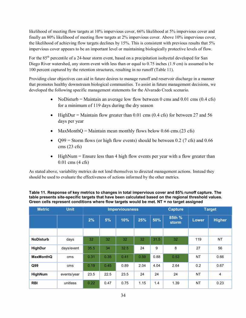
34

likelihood of meeting flow targets at 10% impervious cover, 66% likelihood at 5% impervious cover and finally an 80% likelihood of meeting flow targets at 2% impervious cover. Above 10% impervious cover, the likelihood of achieving flow targets declines by 15%. This is consistent with previous results that 5% impervious cover appears to be an important level or maintaining biologically protective levels of flow.

For the 85th percentile of a 24-hour storm event, based on a precipitation isohyetal developed for San Diego River watershed, any storm event with less than or equal to 0.75 inches (1.9 cm) is assumed to be 100 percent captured by the retention structures, resulting in no runoff (Table 11).

Providing clear objectives can aid in future desires to manage runoff and reservoir discharge in a manner that promotes healthy downstream biological communities. To assist in future management decisions, we developed the following specific management statements for the Alvarado Creek scenario.

NoDisturb = Maintain an average low flow between 0 cms and 0.01 cms (0.4 cfs) for a minimum of 119 days during the dry season

HighDur = Maintain flow greater than 0.01 cms (0.4 cfs) for between 27 and 56 days per year

MaxMonthQ = Maintain mean monthly flows below 0.66 cms.(23 cfs)

Q99 = Storm flows (or high flow events) should be between 0.2 (7 cfs) and 0.66 cms (23 cfs)

HighNum = Ensure less than 4 high flow events per year with a flow greater than 0.01 cms (4 cfs)

As stated above, variability metrics do not lend themselves to directed management actions. Instead they should be used to evaluate the effectiveness of actions informed by the other metrics.

Table 11. Response of key metrics to changes in total impervious cover and 85% runoff capture. The table presents site-specific targets that have been calculated based on the regional threshold values. Green cells represent conditions where flow targets would be met. NT = no target assigned

Metric Unit Imperviousness Capture Target

2% 5% 10% 25% 50% 85th % storm Lower Higher

NoDisturb days 32 32 32 32 31.5 32 119 NT

HighDur days/event 35.5 34 32.5 24 9 8 27 56

MaxMonthQ cms 0.31 0.35 0.41 0.59 0.88 0.53 NT 0.66

Q99 cms 0.19 0.45 0.89 2.04 4.04 2.64 0.2 0.67

HighNum events/year 23.5 22.5 23.5 24 24 24 NT 4

RBI unitless 0.22 0.47 0.75 1.15 1.4 1.39 NT 0.23

35

IMPLICATIONS AND RECOMMENDATIONS The goal of this project was to demonstrate how regional flow-ecology relationships can be used to inform instream environmental flow properties necessary to meet ecological benchmarks as defined by measures of benthic macroinvertebrate community composition and structure. These target flows can be used to help establish goals for use in hydromodification management, nutrient numeric endpoints, and freshwater bioobjectives. They can also be used to develop performance targets for management actions, BMPs, etc. This case study allowed us to develop a framework for implementing regionally derived flow–ecology relationships to inform local management decisions. The stakeholder-focused process allowed us to identify technical and practical benefits and challenges associated with the approach that can inform future implementation efforts.

Utility of the regional flow-ecology approach based on the ELOHA framework A major objective of this case study was to evaluate the ability to apply the flow–ecology relationships derived from the regional analysis to inform local watershed-scale decisions. Our results illustrate that several of the stated advantages of the ELOHA approach aid in such watershed-scale application. The ability to apply regionally derived flow thresholds to inform local decisions is a major advantage of the ELOHA approach. This eliminates the need to develop local flow–ecology relationships for every stream of interest, as is the case in more traditional instream flow methods (Beecher et al. 2010, McClain et al. 2014). The tools developed through the regional analysis provided readily transferable tools for local stakeholders to produce measures of hydrologic change (i.e., delta H) for any location of interest and to explore how those values would change under different land use or management scenarios. This had the dual benefit of allowing for robust analysis and providing a vehicle for stakeholder engagement in setting management priorities related to instream flow, an important cornerstone of the ELOHA approach.

Use of the predictive CSCI index in our regional flow-ecology analysis took advantage of the available bioassessment data and provided an easy way to provide measures of biological change (delta B), which has been a challenge for past ELOHA applications (e.g., McManamay et al. 2013). Developing the regional flow–ecology relationships and applying them at the local scale would not have been possible without the regional bioassessment data and the existence of the predictive scoring tool (Mazor et al. 2016). Large regional data sets provide sufficient sample size to develop statistically meaningful flow-ecology relationships in spite of the inherent “noise” in the data associated with other co-occurring factors that interact with flow to affect biological community condition (Solans and Jalon 2016). The predictive scoring tool is a measure of biological condition relative to expected reference conditions and thus provides a readily available measure of biological change (delta B) at every site. The availability of similar data and tools should be a major consideration for other efforts interested in developing similar regional approaches.

Other important elements of the ELOHA approach are the inclusion of a broad suite of hydrologic metrics that relate to ecologically relevant biological metrics through hypothesized flow–ecology relationships. Our seven priority flow metrics included two measures of magnitude, two of duration, two measures of variability, and one of frequency. This combination ensures that all elements of the hydrograph will be addressed through flow management. The selected metrics have hypothesized relationships that affect macroinvertebrate communities, allowing us to communicate their ecological relevance to managers and local stakeholders (Table 12). They are also amenable to management and minimize redundancy between metrics (Table 13). Interestingly, our metrics are similar to those identified by DeGasperi et al. (2009) who found that decreases in macroinvertebrate indices in urbanizing watersheds in the Puget Sound area

36

of Washington were associated with changes to the number and duration of high and low flow events, and flow flashiness. It is important to note, however, that hypothesized relationships for both this study and other similar studies were derived through statistical analysis of regional bioassessment data sets. Additional mechanistic studies will be important to validate these relationships and confirm their ecological relevancy. As such studies are completed, they can be used to refine flow management targets based on improved understanding of the flow–ecology relationships.

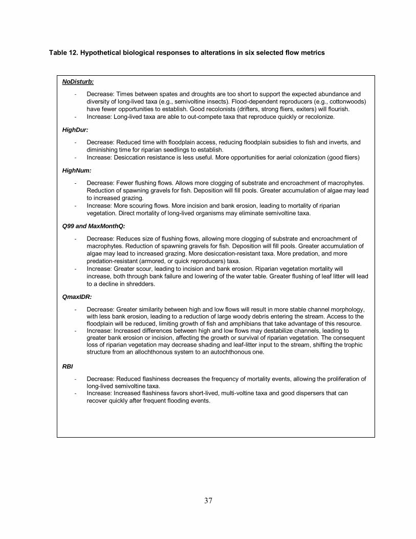
37

Table 12. Hypothetical biological responses to alterations in six selected flow metrics

NoDisturb:

- Decrease: Times between spates and droughts are too short to support the expected abundance and diversity of long-lived taxa (e.g., semivoltine insects). Flood-dependent reproducers (e.g., cottonwoods) have fewer opportunities to establish. Good recolonists (drifters, strong fliers, exiters) will flourish.

- Increase: Long-lived taxa are able to out-compete taxa that reproduce quickly or recolonize.

HighDur:

- Decrease: Reduced time with floodplain access, reducing floodplain subsidies to fish and inverts, and diminishing time for riparian seedlings to establish.

- Increase: Desiccation resistance is less useful. More opportunities for aerial colonization (good fliers)

HighNum:

- Decrease: Fewer flushing flows. Allows more clogging of substrate and encroachment of macrophytes. Reduction of spawning gravels for fish. Deposition will fill pools. Greater accumulation of algae may lead to increased grazing.

- Increase: More scouring flows. More incision and bank erosion, leading to mortality of riparian vegetation. Direct mortality of long-lived organisms may eliminate semivoltine taxa.

Q99 and MaxMonthQ:

- Decrease: Reduces size of flushing flows, allowing more clogging of substrate and encroachment of macrophytes. Reduction of spawning gravels for fish. Deposition will fill pools. Greater accumulation of algae may lead to increased grazing. More desiccation-resistant taxa. More predation, and more predation-resistant (armored, or quick reproducers) taxa.

- Increase: Greater scour, leading to incision and bank erosion. Riparian vegetation mortality will increase, both through bank failure and lowering of the water table. Greater flushing of leaf litter will lead to a decline in shredders.

QmaxIDR:

- Decrease: Greater similarity between high and low flows will result in more stable channel morphology, with less bank erosion, leading to a reduction of large woody debris entering the stream. Access to the floodplain will be reduced, limiting growth of fish and amphibians that take advantage of this resource.

- Increase: Increased differences between high and low flows may destabilize channels, leading to greater bank erosion or incision, affecting the growth or survival of riparian vegetation. The consequent loss of riparian vegetation may decrease shading and leaf-litter input to the stream, shifting the trophic structure from an allochthonous system to an autochthonous one.

RBI

- Decrease: Reduced flashiness decreases the frequency of mortality events, allowing the proliferation of long-lived semivoltine taxa.

- Increase: Increased flashiness favors short-lived, multi-voltine taxa and good dispersers that can recover quickly after frequent flooding events.

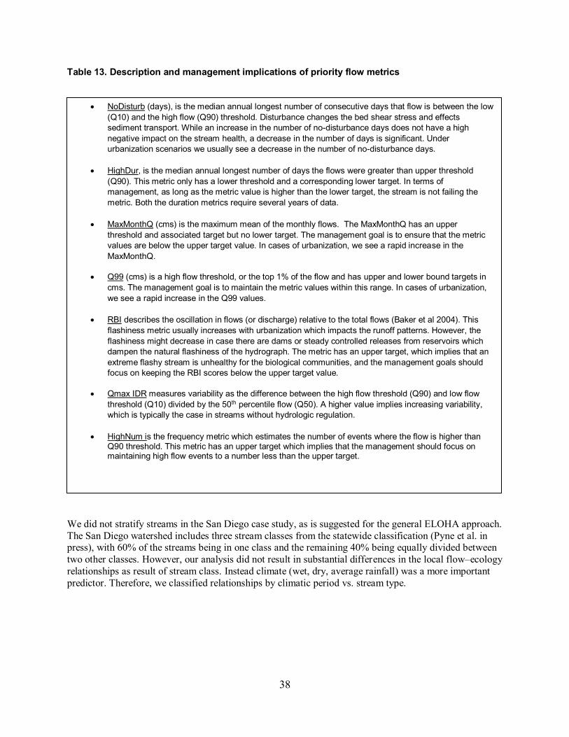
38

Table 13. Description and management implications of priority flow metrics

We did not stratify streams in the San Diego case study, as is suggested for the general ELOHA approach. The San Diego watershed includes three stream classes from the statewide classification (Pyne et al. in press), with 60% of the streams being in one class and the remaining 40% being equally divided between two other classes. However, our analysis did not result in substantial differences in the local flow–ecology relationships as result of stream class. Instead climate (wet, dry, average rainfall) was a more important predictor. Therefore, we classified relationships by climatic period vs. stream type.

NoDisturb (days), is the median annual longest number of consecutive days that flow is between the low (Q10) and the high flow (Q90) threshold. Disturbance changes the bed shear stress and effects sediment transport. While an increase in the number of no-disturbance days does not have a high negative impact on the stream health, a decrease in the number of days is significant. Under urbanization scenarios we usually see a decrease in the number of no-disturbance days.

HighDur, is the median annual longest number of days the flows were greater than upper threshold (Q90). This metric only has a lower threshold and a corresponding lower target. In terms of management, as long as the metric value is higher than the lower target, the stream is not failing the metric. Both the duration metrics require several years of data.

MaxMonthQ (cms) is the maximum mean of the monthly flows. The MaxMonthQ has an upper threshold and associated target but no lower target. The management goal is to ensure that the metric values are below the upper target value. In cases of urbanization, we see a rapid increase in the MaxMonthQ.

Q99 (cms) is a high flow threshold, or the top 1% of the flow and has upper and lower bound targets in cms. The management goal is to maintain the metric values within this range. In cases of urbanization, we see a rapid increase in the Q99 values.

RBI describes the oscillation in flows (or discharge) relative to the total flows (Baker et al 2004). This flashiness metric usually increases with urbanization which impacts the runoff patterns. However, the flashiness might decrease in case there are dams or steady controlled releases from reservoirs which dampen the natural flashiness of the hydrograph. The metric has an upper target, which implies that an extreme flashy stream is unhealthy for the biological communities, and the management goals should focus on keeping the RBI scores below the upper target value.

Qmax IDR measures variability as the difference between the high flow threshold (Q90) and low flow threshold (Q10) divided by the 50th percentile flow (Q50). A higher value implies increasing variability, which is typically the case in streams without hydrologic regulation.

HighNum is the frequency metric which estimates the number of events where the flow is higher than Q90 threshold. This metric has an upper target which implies that the management should focus on maintaining high flow events to a number less than the upper target.

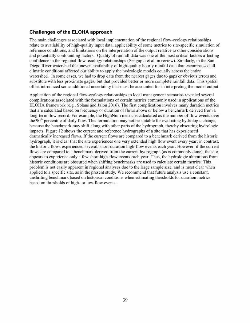
39

Challenges of the ELOHA approach The main challenges associated with local implementation of the regional flow-ecology relationships relate to availability of high-quality input data, applicability of some metrics to site-specific simulation of reference conditions, and limitations on the interpretation of the output relative to other considerations and potentially confounding factors. Quality of rainfall data was one of the most critical factors affecting confidence in the regional flow–ecology relationships (Sengupta et al. in review). Similarly, in the San Diego River watershed the uneven availability of high-quality hourly rainfall data that encompassed all climatic conditions affected our ability to apply the hydrologic models equally across the entire watershed. In some cases, we had to drop data from the nearest gages due to gaps or obvious errors and substitute with less proximate gages, but that provided better or more complete rainfall data. This spatial offset introduced some additional uncertainty that must be accounted for in interpreting the model output.

Application of the regional flow-ecology relationships to local management scenarios revealed several complications associated with the formulations of certain metrics commonly used in applications of the ELOHA framework (e.g., Solans and Jalon 2016). The first complication involves many duration metrics that are calculated based on frequency or duration of flows above or below a benchmark derived from a long-term flow record. For example, the HighNum metric is calculated as the number of flow events over the 90th percentile of daily flow. This formulation may not be suitable for evaluating hydrologic change, because the benchmark may shift along with other parts of the hydrograph, thereby obscuring hydrologic impacts. Figure 12 shows the current and reference hydrographs of a site that has experienced dramatically increased flows. If the current flows are compared to a benchmark derived from the historic hydrograph, it is clear that the site experiences one very extended high flow event every year; in contrast, the historic flows experienced several, short-duration high-flow events each year. However, if the current flows are compared to a benchmark derived from the current hydrograph (as is commonly done), the site appears to experience only a few short high-flow events each year. Thus, the hydrologic alterations from historic conditions are obscured when shifting benchmarks are used to calculate certain metrics. This problem is not easily apparent in regional analyses due to the large sample size, and is most clear when applied to a specific site, as in the present study. We recommend that future analysis use a constant, unshifting benchmark based on historical conditions when estimating thresholds for duration metrics based on thresholds of high- or low-flow events.

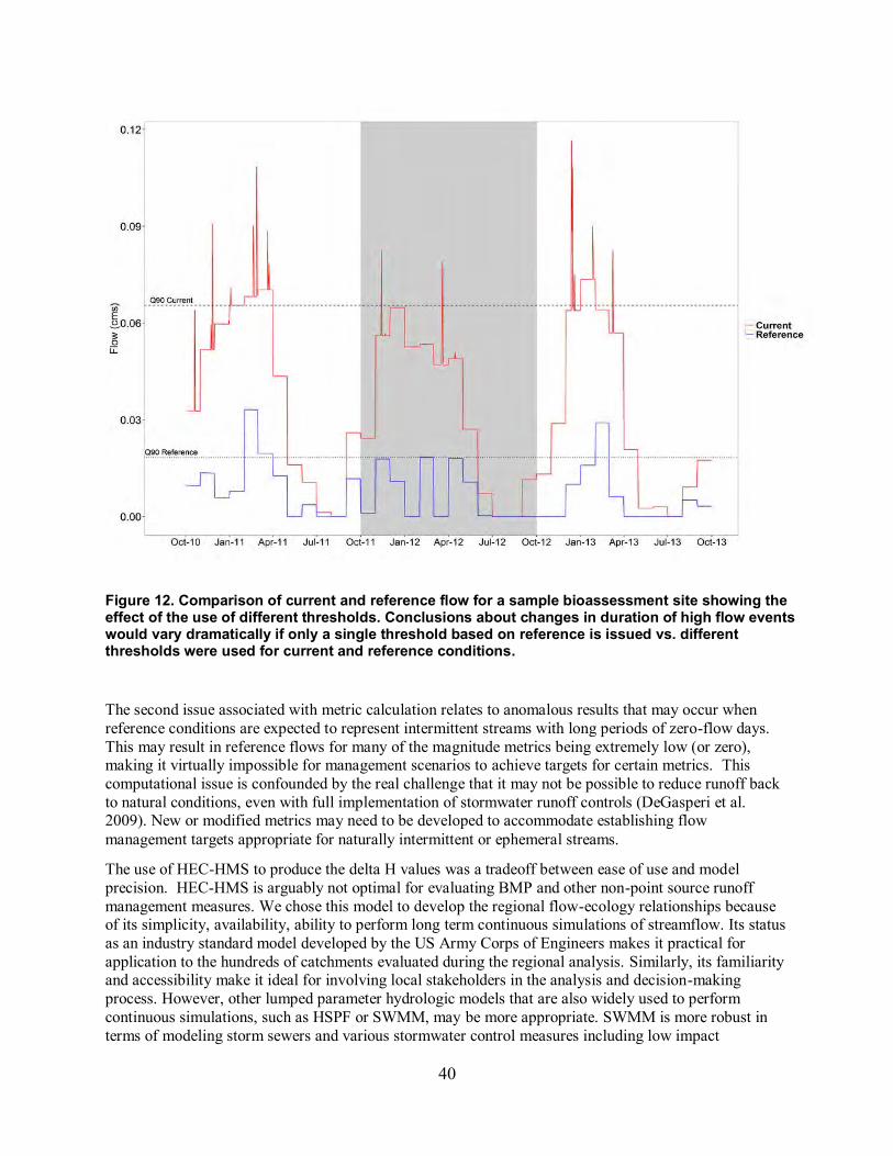
40

Figure 12. Comparison of current and reference flow for a sample bioassessment site showing the effect of the use of different thresholds. Conclusions about changes in duration of high flow events would vary dramatically if only a single threshold based on reference is issued vs. different thresholds were used for current and reference conditions.

The second issue associated with metric calculation relates to anomalous results that may occur when reference conditions are expected to represent intermittent streams with long periods of zero-flow days. This may result in reference flows for many of the magnitude metrics being extremely low (or zero), making it virtually impossible for management scenarios to achieve targets for certain metrics. This computational issue is confounded by the real challenge that it may not be possible to reduce runoff back to natural conditions, even with full implementation of stormwater runoff controls (DeGasperi et al. 2009). New or modified metrics may need to be developed to accommodate establishing flow management targets appropriate for naturally intermittent or ephemeral streams.

The use of HEC-HMS to produce the delta H values was a tradeoff between ease of use and model precision. HEC-HMS is arguably not optimal for evaluating BMP and other non-point source runoff management measures. We chose this model to develop the regional flow-ecology relationships because of its simplicity, availability, ability to perform long term continuous simulations of streamflow. Its status as an industry standard model developed by the US Army Corps of Engineers makes it practical for application to the hundreds of catchments evaluated during the regional analysis. Similarly, its familiarity and accessibility make it ideal for involving local stakeholders in the analysis and decision-making process. However, other lumped parameter hydrologic models that are also widely used to perform continuous simulations, such as HSPF or SWMM, may be more appropriate. SWMM is more robust in terms of modeling storm sewers and various stormwater control measures including low impact

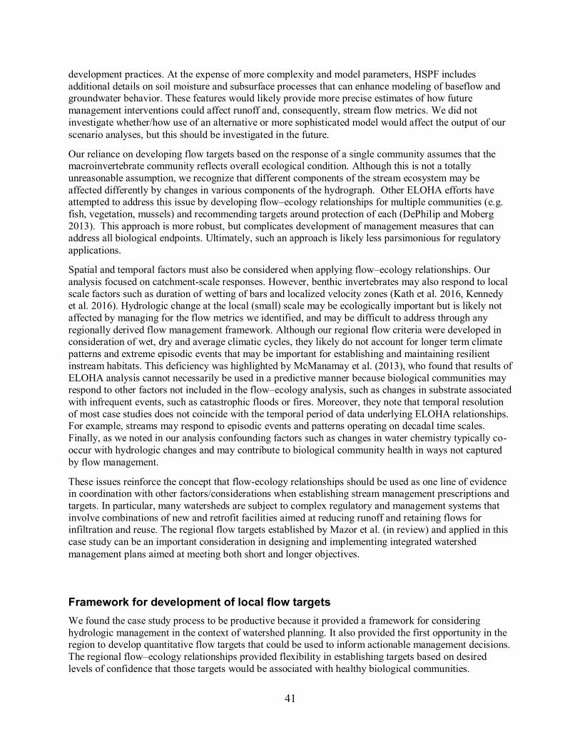
41

development practices. At the expense of more complexity and model parameters, HSPF includes additional details on soil moisture and subsurface processes that can enhance modeling of baseflow and groundwater behavior. These features would likely provide more precise estimates of how future management interventions could affect runoff and, consequently, stream flow metrics. We did not investigate whether/how use of an alternative or more sophisticated model would affect the output of our scenario analyses, but this should be investigated in the future.

Our reliance on developing flow targets based on the response of a single community assumes that the macroinvertebrate community reflects overall ecological condition. Although this is not a totally unreasonable assumption, we recognize that different components of the stream ecosystem may be affected differently by changes in various components of the hydrograph. Other ELOHA efforts have attempted to address this issue by developing flow–ecology relationships for multiple communities (e.g. fish, vegetation, mussels) and recommending targets around protection of each (DePhilip and Moberg 2013). This approach is more robust, but complicates development of management measures that can address all biological endpoints. Ultimately, such an approach is likely less parsimonious for regulatory applications.

Spatial and temporal factors must also be considered when applying flow–ecology relationships. Our analysis focused on catchment-scale responses. However, benthic invertebrates may also respond to local scale factors such as duration of wetting of bars and localized velocity zones (Kath et al. 2016, Kennedy et al. 2016). Hydrologic change at the local (small) scale may be ecologically important but is likely not affected by managing for the flow metrics we identified, and may be difficult to address through any regionally derived flow management framework. Although our regional flow criteria were developed in consideration of wet, dry and average climatic cycles, they likely do not account for longer term climate patterns and extreme episodic events that may be important for establishing and maintaining resilient instream habitats. This deficiency was highlighted by McManamay et al. (2013), who found that results of ELOHA analysis cannot necessarily be used in a predictive manner because biological communities may respond to other factors not included in the flow–ecology analysis, such as changes in substrate associated with infrequent events, such as catastrophic floods or fires. Moreover, they note that temporal resolution of most case studies does not coincide with the temporal period of data underlying ELOHA relationships. For example, streams may respond to episodic events and patterns operating on decadal time scales. Finally, as we noted in our analysis confounding factors such as changes in water chemistry typically co-occur with hydrologic changes and may contribute to biological community health in ways not captured by flow management.

These issues reinforce the concept that flow-ecology relationships should be used as one line of evidence in coordination with other factors/considerations when establishing stream management prescriptions and targets. In particular, many watersheds are subject to complex regulatory and management systems that involve combinations of new and retrofit facilities aimed at reducing runoff and retaining flows for infiltration and reuse. The regional flow targets established by Mazor et al. (in review) and applied in this case study can be an important consideration in designing and implementing integrated watershed management plans aimed at meeting both short and longer objectives.

Framework for development of local flow targets We found the case study process to be productive because it provided a framework for considering hydrologic management in the context of watershed planning. It also provided the first opportunity in the region to develop quantitative flow targets that could be used to inform actionable management decisions. The regional flow–ecology relationships provided flexibility in establishing targets based on desired levels of confidence that those targets would be associated with healthy biological communities.

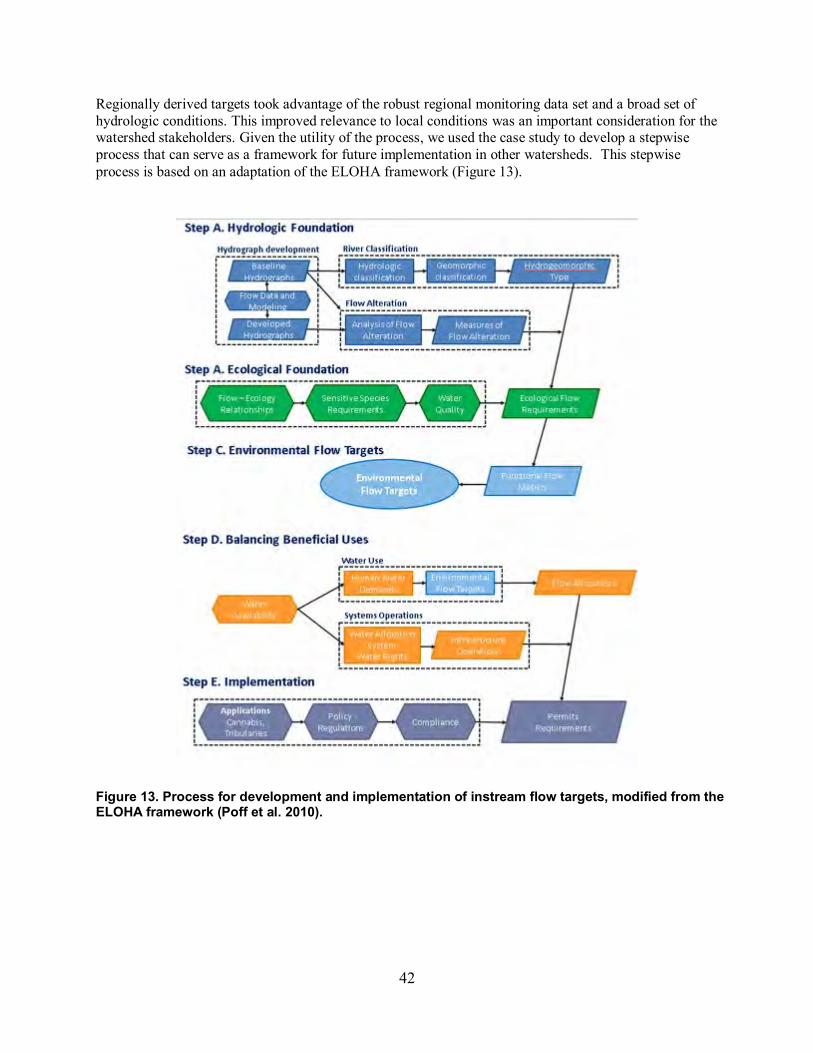
42

Regionally derived targets took advantage of the robust regional monitoring data set and a broad set of hydrologic conditions. This improved relevance to local conditions was an important consideration for the watershed stakeholders. Given the utility of the process, we used the case study to develop a stepwise process that can serve as a framework for future implementation in other watersheds. This stepwise process is based on an adaptation of the ELOHA framework (Figure 13).

Figure 13. Process for development and implementation of instream flow targets, modified from the ELOHA framework (Poff et al. 2010).

43

Based on the framework in Figure 13, we identified the following steps that can be followed if other groups wish to pursue similar efforts to develop flow management recommendations:

Step 1: Determine what hydrologic class the stream of interest is in

Step 2: Identify management needs, regulatory objectives, or other targets

Step 3: Compile local data

Contemporary and proposed future land use Information on contemporary and proposed water capture, storage, diversion, discharge,

and other water management Local rainfall data at hourly time intervals (data must be checked to ensure sufficient

quality and duration, at least ten years that encompass wet, dry, average rainfall conditions)

Step 4: Divide watershed in subbasins for analysis based on hydrology and management needs

Step 5: Select appropriate model(s) for catchments of interest using regional model selection tool

Step 6: Model both contemporary and natural hydrology for each catchment

Step 7: Calculate delta H metrics for each reach/node

Step 8: Select priority metrics and targets based on the following:

Recommendations from the regional ELOHA analysis Relevance to local management needs Ability to influence through management measures

Step 9: Determine temporal factors associated with the targets

Seasonality Persistence/duration Frequency (e.g. always, every X years)

Step 10: Evaluate various management scenarios relative to targets identified in Step 8

Step 11: Explore potential related or confounding factors (e.g. water quality, substrate)

Step 12: Develop recommended actions to achieve flow targets

Relate actions to specific hydrologic modifications, e.g. diversion rates

Step 13: Relate flow metrics and targets to monitoring design, locations, and indicators

Step 14: Determine adaptive management actions that will be triggered if targets are not met

Informing management decisions Stakeholder participation was critical in identifying scenarios and interpreting how the results of the analysis can be used to inform management action. Stakeholders identified the following desired applications for flow targets, which helped define our analysis:

44

Identify priority management sites based on biological and hydrologic condition

Use results to inform BMP/LID selection

Identify areas were flow management has potential to improve CSCI scores

Explore implication of future management of reservoirs for multiple benefits, e.g. water quality and water supply

These desired uses shaped our ultimate products. For example, we developed the overall composite index of hydrologic alteration in direct response to stakeholder desire to holistically assess the watershed for areas most vulnerable to future hydrologic alteration. Not surprisingly, the degree of hydrologic modification was correlated with impervious cover. We found that hydrologic alteration generally occurred in catchments with greater than 5% total impervious cover, which is similar to other studies that have shown that channel degradation to due to hydromodification occurs at relatively low levels of imperviousness (Hawley et al. 2012, Vietz et al. 2016). Similarly, the map of hydrologic management categories was identified as one of the most useful products for planning purposes because it allows stakeholders to prioritize areas for protection and for flow management.

We were able to demonstrate the utility of applying the flow-ecology relationships to inform management for both point source and non-point source management scenarios. For both the reservoir management scenario and the urban runoff management scenario, we were able to determine a range at which hydrologic management may facilitate recovery of impacted biological communities.

Lessons learned for future implementation Future efforts can built on the experiences from this case study and continue to refine an iterative process of developing flow targets that are scientifically defensible, practical (i.e., can lead to management actions), and consistent with local stakeholder needs. Key lessons learned from this effort include:

1. Include a broad set of engaged stakeholders, including regulatory agencies, municipalities, water agencies, non-governmental organizations, and researchers. This ensures a broad perspective in the deliberations and increases the likelihood of developing balanced recommendations.

2. Invest in educating the stakeholders early in the process on the underlying science and the rationale behind how regional flow targets were developed. This promotes engagement and fosters creative solutions to the complex challenges of flow management.

3. Invest the time to compile high quality local data sources and show how local data can be used in the evaluation process. Identify the areas were future date collection can most improve outputs of the flow–ecology analysis (e.g., local rainfall data, more refined land use, water quality data). This can inform future monitoring.

4. Develop documentation that clearly illustrates how the products of the flow–ecology analysis can be used in the context of existing regulatory or management programs.

The San Diego River implementation case study also produced several technical recommendations that can improve our ability to apply flow-ecology relationships to manage southern California streams:

1. Several flow metrics, particularly those associated with flow duration, may require modification for use in streams where the natural condition is intermittent or ephemeral.

45

Natural intermittency poses fewer issues when developing regional flow-ecology relationships based on hundreds of sites. However, application of the resultant thresholds to specific streams that may have been naturally intermittent can lead to erroneous results.

2. Metrics associated with flow durations should be calculated on a single threshold value based on reference conditions. Estimating hydrologic change based on a moving threshold estimated separately for current and reference conditions may produce erroneous results.

3. Need to improve the representation of the drainage system to provide a more accurate hydrologic foundation for analysis. This would ultimately include improved mapping of discharges, diversions, stormwater control facilities, LID, etc. for incorporation into modeling scenarios and effects.

4. Consider expanding the analysis to include additional elements in future case studies

Include other stream or water body types

Include other indicators (e.g. algae)

Explore how consistent/transferable findings are from one watershed to another

Explore application in watersheds that cross jurisdictional boundaries

The original authors of the ELOHA framework promote the idea that flow targets derived by statistical analysis are a starting point. Targets should be iteratively refined using additional monitoring data, professional judgement and consideration of all complementary and competing factors necessary to develop flow standards that can address often divergent interests. The San Diego River case study provides an illustration of how watershed stakeholders are critical partners in the process. Resultant flow standards provide a starting point for developing agreed upon, adaptive flow management programs that can protect intact waterbodies and restore those that are currently impacted.

46

LITERATURE CITED Baker, D.B., Richards, R.P, Loftus, T.T, and Kramer, J.W. 2004. A new flashiness index: Characteristics and applications to Midwestern Rivers and streams. JAWRA Journal of the American Water Resources Association, 40: 503–522. doi:10.1111/j.1752-

Beecher, H.A., B.A. Caldwell, S.B. DeMond, D. Seiler, S.N. Boessow. 2010. An Empirical Assessment of PHABSIM Using Long-Term Monitoring of Coho Salmon Smolt Production in Bingham Creek,Washington, North American Journal of Fisheries Management, 30: 6, 1529 — 1543: DOI: 10.1577/M10-020.1

Buchanan,C, H.L.N. Moltz, H.C. Haywood, J.B. Palmer, A.N. Griggs. 2013. A test of The Ecological Limits of Hydrologic Alteration (ELOHA) method for determining environmental flows in the Potomac River basin, U.S.A. Freshwater Biology (2013) 58, 2632–2647

Bunn, S.E. and A.H. Arthington. 2002, Basic principles and ecological consequences of altered flow regimes for aquatic biodiversity: Environmental Management, v. 30, no. 4, p. 492–507.

Colwell R.K. 1974. Predictability, constancy, and contingency of periodic phenomena. Ecology 55(5): 1148-53.

DeGasperi C.L., H.B. Berge, K.R. Whiting, J.J. Burkey, J.L. Cassin and R.R. Fuerstenberg. 2009. Linking Hydrologic Alteration to Biological Impairment in Urbanizing Streams of the Puget Lowland, Washington, USA. Journal of the American Water Resources Association (JAWRA) 45(2):512-533. DOI: 10.1111/j.1752-1688.2009.00306.x

DePhilip, M. and T. Moberg. 2010. Ecosystem flow recommendations for the Susquehanna River Basin. The Nature Conservancy. Harrisburg, PA.

DePhilip, M. and T. Moberg. 2013. Ecosystem flow recommendations for the Upper Ohio River basin in western Pennsylvania. The Nature Conservancy. Harrisburg, PA.

Elith J., J.R. Leathwick and T. Hastie. 2008. A working guide to boosted regression trees. Journal of Animal Ecology 77: 802–813.

Friedman, J.H. 2001. Greedy function approximation: A gradient boosting machine. The Annals of Statistics 29: 1189–1232.

Hawley, R.J. and B.P. Bledsoe. 2011. How do flow peaks and durations change in suburbanizing semi-arid watersheds? A southern California case study. Journal of Hydrology 405:69–82

Hawley, R.J., B.P. Bledsoe, E.D. Stein and B.E. Haines. 2012. Channel Evolution Model of Response to Urbanization in Southern California. Journal of the American Water Resources Association 48(4):722—744.

Horvitz, D.G. and D.J. Thompson. 1952. A generalization of sampling without replacement from a finite universe. Journal of the American Statistical Association 47:663-685.

Kath J., E. Harrison, B.J. Kefford, L. Moore, P.J. Wood, R.B. Schäfer, F. Dyer. 2016. Looking beneath the surface: using hydrogeology and traits to explain flow variability effects on stream macroinvertebrates. Ecohydrology (online). DOI: 10.1002/eco.1741

Kennedy T.A., J.D. Muehlbauer, C.B. Yackulic, D.A. Lytle, S.W. Miller, K.L. Dibble, E.W. Kortenhoeven, A.N. Metcalfe, C.V. Baxter. 2016. Flow Management for Hydropower Extirpates Aquatic Insects, Undermining River Food Webs. BioScience (online). Doi:10.1093/biosci/biw059

47

Kincaid, T.M. and A.R. Olsen. 2013. Spsurvey: Spatial survey design and analysysis. R package version 2.6. R Foundation for Statistical Computing. Vienna, Austria.

King County. 2012. Stormwater Retrofit Analysis for Juanita Creek Basin in the Lake Washington Watershed. Ecology Grant: G0800618. Prepared by J Burkey, M Wilgus H Berge. King County Department of Natural Resources and Parks. Water and Land Resources Division.Seattle, Washington.

Konrad C.P. and D.B. Booth. 2005. Hydrologic Changes in Urban Streams and Their Ecological Significance. American Fisheries Society Symposium 47:157–177

Konrad C,P,, A,M,D. Brasher, J.T. May. 2008. Assessing streamflow characteristics as limiting factors on benthic invertebrate assemblages in streams across the western United States. Freshwater Biology, 53:1983–1998.

Mazor, R.D., J. May, A. Sengupta, K. McCune, E.D. Stein. (In review). Setting hydrologic targets to support biological integrity. Freshwater Biology

Mazor, R.D. 2015. Bioassessment of Streams in Southern California: A Report on the First Five Years of the Stormwater Monitoring Coalition’s Regional Stream Survey. Southern California Coastal Water Research Project Technical Report #844

Mazor, R.D., A.C. Rehn, P.R. Ode, M. Engeln, K.C. Schiff, E.D. Stein, D.J. Gillett, D.B. Herbst, C.P. Hawkins. 2016. Bioassessment in complex environments: designing an index for consistent meaning in different settings. Freshwater Science. 35(1):249–271. DOI: 10.1086/684130

Mazor, R.D., K. Schiff, K. Ritter, A. Rehn, P. Ode. 2010. Bioassessment tools in novel habitats: An evaluation of indices and sampling methods in low-gradient streams in California. Environmental Monitoring and Assessment 167:91-104.

McClain, M.E., A.L. Subalusky, E.P. Anderson, S.B. Dessu, A.M. Melesse, P.M. Ndomba, J.O.D. Mtamba, R.A. Tamatamah, C. Mligo. 2014. Comparing flow regime, channel hydraulics and biological communities to infer flow–ecology relationships in the Mara River of Kenya and Tanzania. Hydrological Sciences Journal, 59 (3–4), 801–819.

McManamay, R.A., D.J. Orth, C.A. Dolloff, D.C. Mathews. 2013. Application of the ELOHA Framework to Regulated Rivers in the Upper Tennessee River Basin: A Case Study. Environmental Management 51:1210–1235: DOI 10.1007/s00267-013-0055-3

Moriasi, D.N, J.G. Arnold, M.W. Van Liew, R.L. Bingner, R.D. Harmel, T.L. Veith. 2007. Model evaluation guidelines for systematic quantification of accuracy in watershed simulations. Transactions of the ASABE 50(3):885-900

Morley, S.A., J.R. Karr. 2002. Assessing and Restoring the Health of Urban Streams in the Puget Sound Basin. Conservation Biology 16(6):1498–1509

Naiman, R.J., S.E. Bunn, C. Nilsson, G.E. Petts, G. Pinnay, L.C. Thompson. 2002. Legitimizing fluvial ecosystems as users of water—an overview: Environmental Management, v. 30, no. 4, p. 455–467.

Novak, R., J.G. Kennen, R.W. Abele, C.F. Baschon, D.M. Carlisle, L. Dlugolecki., J.E. Flotermersch, P. Ford, J. Fowler, R. Galer, L.P. Gordon, S.N. Hansen, B. Herbold, T.E. Johnson, J.M. Johnston, C.P. Konrad, B. Leamond, P.W. Seelbach. 2015. Draft: EPA-USGS Technical Report: Protecting Aquatic Life from Effects of Hydrologic Alteration: U.S. Geological Survey Scientific Investigations Report 2015–5160, U.S. Environmental Protection Agency EPA Report

48

822-P-15-002, XX p., http://pubs.usgs.gov/sir/2015/5160/ and http://www2.epa.gov/wqc/aquatic life-ambient-water quality-criteria

Ode PR. 2007. Standard operating procedures for collecting benthic macroinvertebrate samples and associated physical and chemical data for ambient bioassessment in California. Surface Water Ambient Monitoring Program. Sacramento, CA.

Parasiewicz, P. 2009. Habitat Time Series Analysis to Define Flow Augmentation Strategy for the Quinebaug River, Connecticut and Massachusetts, USA. River Research and Applications. Published online in Wiley InterScience (www.interscience.wiley.com) DOI: 10.1002/rra.1066

Peck, D.V.,A.T. Herlihy, B.H. Hill, R.M. Hughes, P.R. Kaufmann, D.J. Klemm, J.M. Lazorchak, F.H. McCormick, S.A. Peterson, P.L. Ringold, T. Magee, and M. Cappaert. 2006. Environmental Monitoring and Assessment Program -Surface Waters Western Pilot Study: Field Operations Manual for Wadeable Streams. EPA/620/R-06/003. U.S. Environmental Protection Agency, Office of Research and Development, Washington, D.C

Peterson, S.A., P. L. Ringold, T Magee, M Cappaert. 2006. Environmental Monitoring and Assessment Program - Surface Waters Western Pilot Study: field operations manual for wadeable streams. EPA/620/R-06/003. US Environmental Protection Agency, Office of Research and Development. Corvallis, OR.

Poff, N.L. and J.K.H. Zimmerman. 2010. Ecological responses to altered flow regimes—A literature review to inform the science and management of environmental flows: Freshwater Biology, v. 55, no. 1, p. 194–205.

Poff, N.L., B. Richter, A.H. Arthington, S.E. Bunn, R.J. Naiman, C. Apse, E. Kendy, A.T. Warner, R. Tharme, B.P. Bledsoe, D. Merritt, R.B. Jacobson, M. Freeman, K. Rogers, J. Henriksen, J. Olden, J. O’Keeffe, M. Acreman. 2010. The ecological limits of hydrologic alteration: A framework for developing regional environmental flow standards. Freshwater Biology 55, 147–170.

Poff, N.L., J.D. Allan, M.B. Bain, J.R. Karr, K.L. Prestegaard, B.D. Richter, R.E. Sparks, J.C. Stromberg. 1997. The natural flow regime—a paradigm for river conservation and restoration: Bioscience, v. 47, no. 11, p. 769–784.

Pyne, M.I., D.M. Carlisle, C.P. Konrad, E.D. Stein. (in press) Classification of California streams using combined deductive and inductive approaches: setting the foundation for analysis of hydrologic alteration. Ecohydrology (in press).

R Core Team. 2016. R: A Language and Environment for Statistical Computing. R Foundation for Statistical Computing. Version 3.2.4. Vienna, Austria.

Richards, A.B. and D.C. Rogers. 2006. List of Freshwater Macroinvertebrate Taxa from California and Adjacent States Including Standard Taxonomic Effort Levels. Southwest Association of Freshwater Invertebrate Taxonomists. Chico, CA.

Richter, B.D., M.M. Davis, C. Apse, C. Konrad. 2011. A presumptive standard for environmental flow protection. River Research and Applications 28(8):1312-1321. DOI: 0.1002/rra.1511

Ridgeway, G. 2015. gbm: Generalized Boosted Regression Models. R package version 2.1.1. https://CRAN.R-project.org/package=gbm

San Diego Geographic Information Source. Digital land use layers. http://www.sangis.org/index.html

49

Scharffenberg, W. A., and M.J. Fleming. Hydrologic Modeling System HEC-HMS: User's Manual. US Army Corps of Engineers, Hydrologic Engineering Center, 2006.

Sengupta A., E.D. Stein, K. McCune, R.D. Mazor, B.P. Bledsoe, S. Adams, C.P. Konrad. (In review). From Gaged to Ungaged: Predicting Flow and Hydrologic Alterations at a Regional Scale for Application to Regional Flow-ecology analyses. Freshwater Biology

Solans, M.A. and D.G. Jalon. 2016. Basic tools for setting environmental flows at the regional scale: application of the ELOHA framework in a Mediterranean river basin. Ecohydrology. DOI: 10.1002/eco.1745

Stevens, D.L. and A.R. Olsen. 2004. Spatially balanced sampling of natural resources. Journal of the American Statistical Association 99:262-278.

U.S. Army Corps of Engineers (ACOE). 2000. Hydrologic Modeling System HEC-HMS U.S. Army Corps of Engineers R&D Technical Reference Manual.

Vietz, G.J., M.J. Sammonds, C.J. Walsh, T.D. Fletcher, I.D. Rutherford, M.J. Stewardson. 2016. Ecologically relevant geomorphic attributes of streams are impaired by even low levels of watershed effective imperviousness. Geomorphology 206:67-78

Xuefeng, C. and Alan Steinman, A. 2009. Event and continuous hydrologic modeling with HEC-HMS. Journal of Irrigation and Drainage Engineering135.1 (2009): 119-124.

Yarnell, S.M., G.E. Petts, J.C. Schmidt, A.A. Whipple, E.E. Beller, C.N. Dahm, P. Goodwin, J.H. Viers. 2015. Functional Flows in Modified Riverscapes: Hydrographs, Habitats and Opportunities. BioScience: doi: 10.1093/biosci/biv102

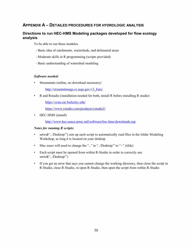
50

APPENDIX A – DETAILED PROCEDURES FOR HYDROLOGIC ANALYSIS

Directions to run HEC-HMS Modeling packages developed for flow ecology analysis

To be able to run these modules

- Basic idea of catchments, watersheds, and delineated areas

- Moderate skills in R programming (scripts provided)

- Basic understanding of watershed modeling

Software needed:

• Streamstats (online, no download necessary)

http://streamstatsags.cr.usgs.gov/v3_beta/

• R and Rstudio (installation needed for both, install R before installing R studio)

https://cran.cnr.berkeley.edu/

https://www.rstudio.com/products/rstudio2/

• HEC-HMS (install)

http://www.hec.usace.army.mil/software/hec-hms/downloads.asp

Notes for running R scripts:

• setwd(“../Desktop/”) sets up each script to automatically read files in the folder Modeling Workshop, as long it is located on your desktop

• Mac users will need to change the “..” in “../Desktop/” to “~” (tilde)

• Each script must be opened from within R-Studio in order to correctly use setwd(“../Desktop/”)

• If you get an error that says you cannot change the working directory, then close the script in R-Studio, close R-Studio, re-open R-Studio, then open the script from within R-Studio

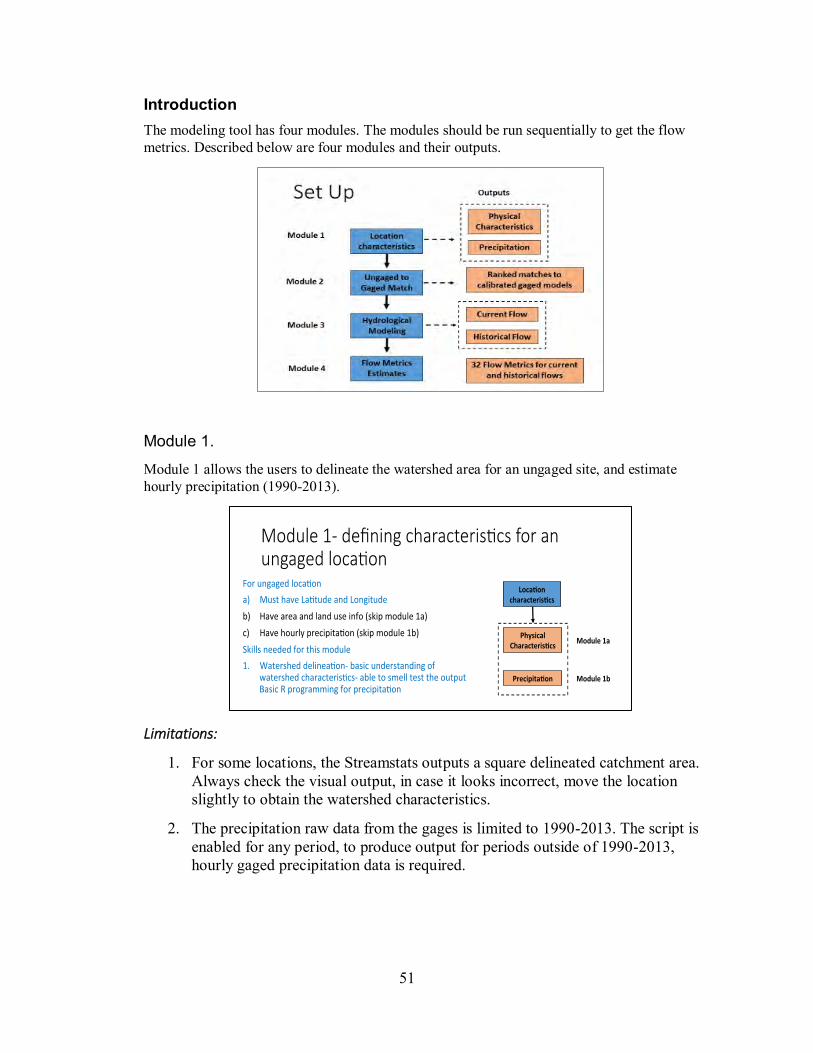
51

Introduction The modeling tool has four modules. The modules should be run sequentially to get the flow metrics. Described below are four modules and their outputs.

Module 1.

Module 1 allows the users to delineate the watershed area for an ungaged site, and estimate hourly precipitation (1990-2013).

Limitations:

1. For some locations, the Streamstats outputs a square delineated catchment area. Always check the visual output, in case it looks incorrect, move the location slightly to obtain the watershed characteristics.

2. The precipitation raw data from the gages is limited to 1990-2013. The script is enabled for any period, to produce output for periods outside of 1990-2013, hourly gaged precipitation data is required.

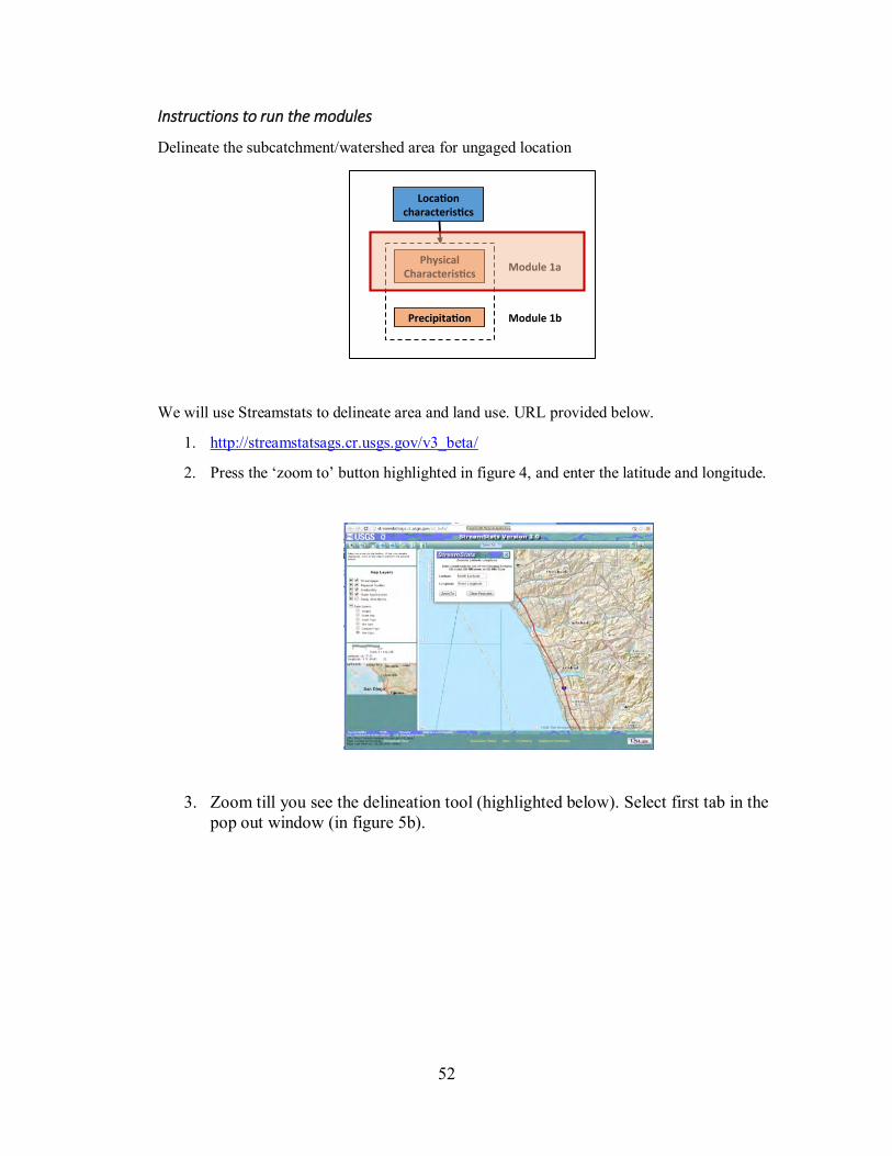
52

Instructions to run the modules

Delineate the subcatchment/watershed area for ungaged location

We will use Streamstats to delineate area and land use. URL provided below.

1. http://streamstatsags.cr.usgs.gov/v3_beta/

2. Press the ‘zoom to’ button highlighted in figure 4, and enter the latitude and longitude.

3. Zoom till you see the delineation tool (highlighted below). Select first tab in the pop out window (in figure 5b).

Loca oncharacteris cs

PhysicalCharacteris cs

Precipita on

Module1a

Module1b

53

4. Select area and imperviousness, and compute

Module 1b. Estimating hourly precipitation

Input files: Modeling Workshop\Inverse Distance\Data\Precip_(YEAR).csv, AssessmentSiteCoord.csv, PrecipStationCoord.csv

Output file: Modeling Workshop\Inverse Distance\Data\Assess_(YEAR).csv

1. We use R Studio to estimate hourly precipitation.

2. To predict flows at the gages, we need hourly precipitation data

3. Daily data is available on PRISM website

4. For better flow predictions, we estimated hourly flow using precipitation data from >200 sites

5. You can use the script for 1990-2013 (and will require raw precipitation data outside this range)

6. Open the file AssessmentSiteCoord.csv, delete the current data in the spreadsheet and enter the data for your site ID, latitude and longitude in the appropriate columns

Loca oncharacteris cs

PhysicalCharacteris cs

Precipita on

Module1a

Module1b

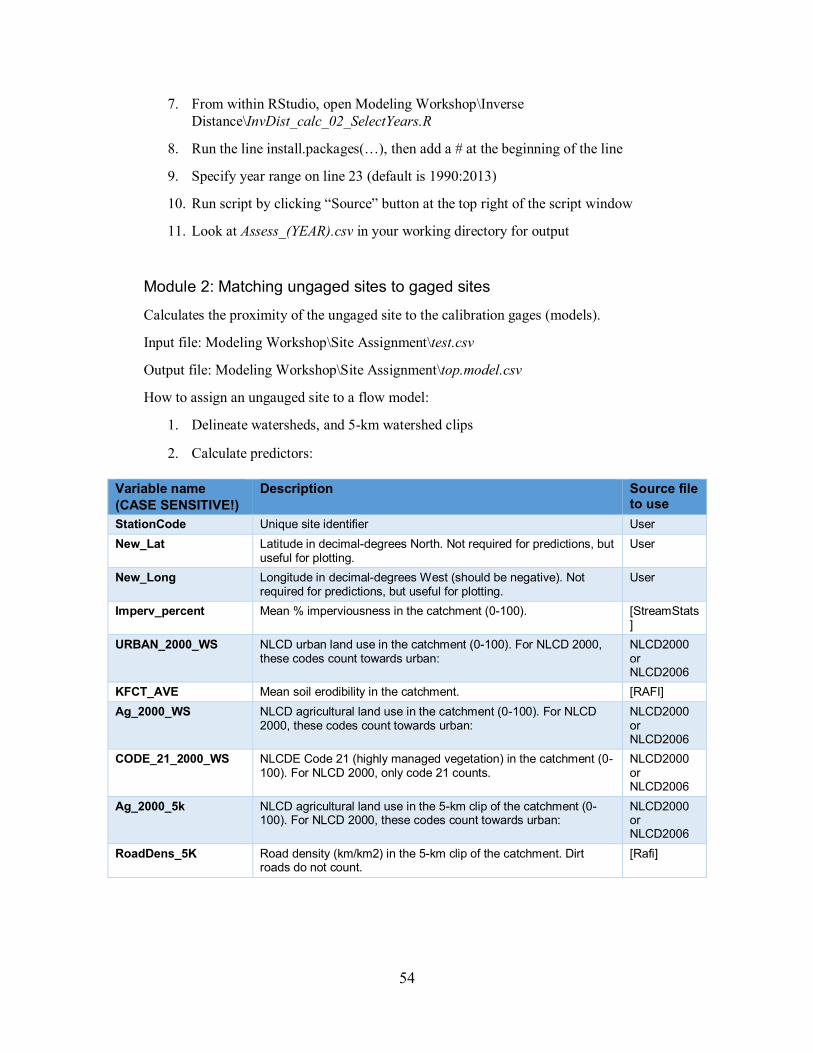
54

7. From within RStudio, open Modeling Workshop\Inverse Distance\InvDist_calc_02_SelectYears.R

8. Run the line install.packages(…), then add a # at the beginning of the line

9. Specify year range on line 23 (default is 1990:2013)

10. Run script by clicking “Source” button at the top right of the script window

11. Look at Assess_(YEAR).csv in your working directory for output

Module 2: Matching ungaged sites to gaged sites

Calculates the proximity of the ungaged site to the calibration gages (models).

Input file: Modeling Workshop\Site Assignment\test.csv

Output file: Modeling Workshop\Site Assignment\top.model.csv

How to assign an ungauged site to a flow model:

1. Delineate watersheds, and 5-km watershed clips

2. Calculate predictors:

Variable name (CASE SENSITIVE!)

Description Source file to use

StationCode Unique site identifier User New_Lat Latitude in decimal-degrees North. Not required for predictions, but

useful for plotting. User

New_Long Longitude in decimal-degrees West (should be negative). Not required for predictions, but useful for plotting.

User

Imperv_percent Mean % imperviousness in the catchment (0-100). [StreamStats]

URBAN_2000_WS NLCD urban land use in the catchment (0-100). For NLCD 2000, these codes count towards urban:

NLCD2000 or NLCD2006

KFCT_AVE Mean soil erodibility in the catchment. [RAFI] Ag_2000_WS NLCD agricultural land use in the catchment (0-100). For NLCD

2000, these codes count towards urban: NLCD2000 or NLCD2006

CODE_21_2000_WS NLCDE Code 21 (highly managed vegetation) in the catchment (0-100). For NLCD 2000, only code 21 counts.

NLCD2000 or NLCD2006

Ag_2000_5k NLCD agricultural land use in the 5-km clip of the catchment (0-100). For NLCD 2000, these codes count towards urban:

NLCD2000 or NLCD2006

RoadDens_5K Road density (km/km2) in the 5-km clip of the catchment. Dirt roads do not count.

[Rafi]

55

1. From within R Studio, open Modeling Workshop\Site Assignment\assigning_testsites_020116.R

2. Currently test.csv has dummy site information; use this as a template for your site info

3. Please see handout for GIS information required for this module

4. top.model.csv is the output file with top matched gage info

Note: Within a year or two automated tools from the State (SWAMP) will calculate the variables, but for now, use GIS to estimate them.

Module 3: Running hydrological model (HEC-HMS) to predict hourly flow

We run the model for current and reference or historical conditions

Output files: Modeling Workshop\Hourly To Daily Flow Conversion\Hourly Flow\SDR_AssessmentSites_Hourly_Current.csv and SDR_AssessmentSites_Hourly_Reference.csv

First we will estimate current flows

1. Navigate to Modeling Workshop\HEC HMS Models\Current Conditions

2. Copy the model folder that is the top matched to your site

3. Save a copy in a new folder

4. Click on HEC-HMS icon on your desktop

5. Click on open folder tab, navigate to your new folder

6. Open file with the .hms extension

7. We need to change 5 parameters- area, imperviousness, time of concentration, storage coefficient and precipitation

8. From the “Compute” tab, right click on “Run 1” then click “Compute”

9. From the “Results” tab, double click “Run 1”, double click “Subbasin-1” then click on “Time-Series Table”

10. A window will appear shortly, from which you will copy all the data in the “Total Flow” column

11. Open the file Modeling Workshop\Hourly To Daily Flow Conversion\Hourly Flow\SDR_AssessmentSites_Hourly_Current.csv, paste the “Total Flow” data in a new column on the right, starting on row 2

12. Put the site name in the first row of this column

13. Remove all the other columns, EXCEPT for your new column, the “Date_Time” column and one additional column of flow data (the metric calculation requires data from at least 2 sites)

Historical flows

1. Navigate to Modeling Workshop\HEC HMS Models\Reference Conditions

56

2. Copy the model folder that is the top matched to your site

3. Save a copy in a new folder

4. Click on HEC-HMS icon on your desktop

5. Click on open folder tab, navigate to your new folder

6. Open file with the .hms extension

7. We need to change 4 parameters- area, time of concentration, storage coefficient and precipitation

8. From the “Compute” tab, right click on “Run 1” then click “Compute”

9. From the “Results” tab, double click “Run 1”, double click “Subbasin-1” then click on “Time-Series Table”

10. A window will appear shortly, from which you will copy all the data in the “Total Flow” column

11. Open the file Modeling Workshop\Hourly To Daily Flow Conversion\Hourly Flow\SDR_AssessmentSites_Hourly_Reference.csv, paste the “Total Flow” data in a new column on the right, starting on row 2

12. Put the site name in the first row of this new column

13. Remove all the other columns, EXCEPT for your new column, the “Date_Time” column and one additional column of flow data (the metric calculation requires data from at least 2 sites)

Module 4. Flow metrics are estimated on daily flow

Convert hourly flow output from HEC-HMS to daily flow

Input files: Modeling Workshop\Hourly To Daily Flow Conversion\Hourly Flow\SDR_AssessmentSites_Hourly_Current.csv and SDR_AssessmentSites_Hourly_Reference.csv

Output files: Modeling Workshop\Hourly To Daily Flow Conversion\Daily Flow\SDR_Assessment_Daily_Current.csv and SDR_Assessment_Daily_Reference.csv

1. From within R Studio, open Metric Workshop\Hourly To Daily Flow Conversion\HourlytoDailyFlow_Current.R

2. Run install.packages(…) line, then add # to the beginning of the line

3. Run script by clicking “Source” button on the top right of the script window

4. Converted daily flow data will be in Modeling Workshop\Hourly To Daily Flow Conversion\Daily Flow\SDR_Assessment_Daily_Current.csv

5. Repeat using Metric Workshop\Hourly To Daily Flow Conversion\HourlytoDailyFlow_Reference.R to produce daily flow data for reference condition hourly flow data

57

Calculate Metrics for Daily Flow Data Input files: Modeling Workshop\Hourly To Daily Flow Conversion\Daily Flow\SDR_AssessmentSites_Daily_Current.csv and SDR_AssessmentSites_Daily_Reference.csv

Output files: Modeling Workshop\Metric Calculation \Results\ Sdr_Current_Metrics.csv and Sdr_Reference_Metrics.csv

1. From within R Studio, open Modeling Workshop\Metric Calculation\KonradMetrics_Current.R

2. Click “Source” button in upper right corner of script window

3. Metric results will be in Modeling Workshop\Metric Calculation\Results\Sdr_Current_Metrics.csv

4. Repeat using Modeling Workshop\Metric Calculation\KonradMetrics_Reference.R to get metric results for reference condition flow data

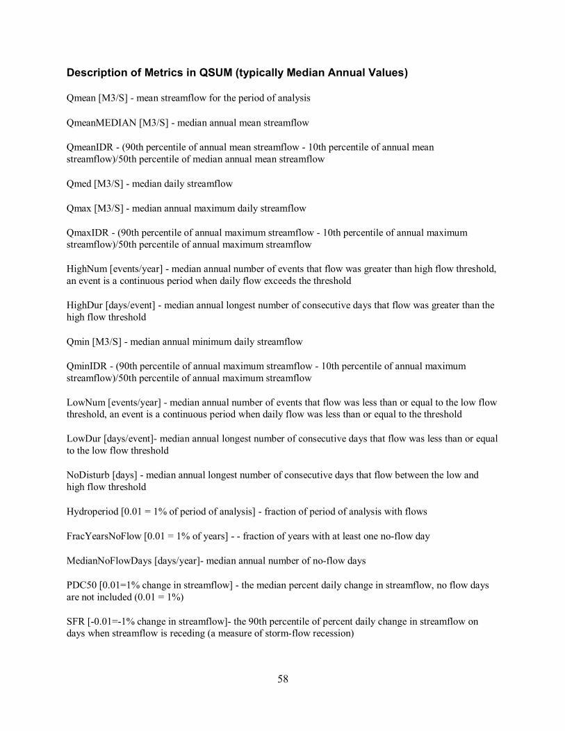
58

Description of Metrics in QSUM (typically Median Annual Values)

Qmean [M3/S] - mean streamflow for the period of analysis

QmeanMEDIAN [M3/S] - median annual mean streamflow

QmeanIDR - (90th percentile of annual mean streamflow - 10th percentile of annual mean streamflow)/50th percentile of median annual mean streamflow

Qmed [M3/S] - median daily streamflow

Qmax [M3/S] - median annual maximum daily streamflow

QmaxIDR - (90th percentile of annual maximum streamflow - 10th percentile of annual maximum streamflow)/50th percentile of annual maximum streamflow

HighNum [events/year] - median annual number of events that flow was greater than high flow threshold, an event is a continuous period when daily flow exceeds the threshold

HighDur [days/event] - median annual longest number of consecutive days that flow was greater than the high flow threshold

Qmin [M3/S] - median annual minimum daily streamflow

QminIDR - (90th percentile of annual maximum streamflow - 10th percentile of annual maximum streamflow)/50th percentile of annual maximum streamflow

LowNum [events/year] - median annual number of events that flow was less than or equal to the low flow threshold, an event is a continuous period when daily flow was less than or equal to the threshold

LowDur [days/event]- median annual longest number of consecutive days that flow was less than or equal to the low flow threshold

NoDisturb [days] - median annual longest number of consecutive days that flow between the low and high flow threshold

Hydroperiod [0.01 = 1% of period of analysis] - fraction of period of analysis with flows

FracYearsNoFlow [0.01 = 1% of years] - - fraction of years with at least one no-flow day

MedianNoFlowDays [days/year]- median annual number of no-flow days

PDC50 [0.01=1% change in streamflow] - the median percent daily change in streamflow, no flow days are not included (0.01 = 1%)

SFR [-0.01=-1% change in streamflow]- the 90th percentile of percent daily change in streamflow on days when streamflow is receding (a measure of storm-flow recession)

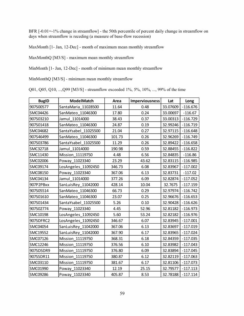
59

BFR [-0.01=-1% change in streamflow] - the 50th percentile of percent daily change in streamflow on days when streamflow is receding (a measure of base-flow recession)

MaxMonth [1- Jan, 12-Dec] - month of maximum mean monthly streamflow

MaxMonthQ [M3/S] - maximum mean monthly streamflow

MinMonth [1- Jan, 12-Dec] - month of minimum mean monthly streamflow

MinMonthQ [M3/S] - minimum mean monthly streamflow

Q01, Q05, Q10, ...,Q99 [M3/S] - streamflow exceeded 1%, 5%, 10%, ..., 99% of the time

BugID ModelMatch Area Imperviousness Lat Long

907S00577 SantaMaria_11028500 11.64 0.48 33.07609 -116.676

SMC04426 SanMateo_11046300 17.80 0.24 33.00697 -116.67

907S03210 Jamul_11014000 38.43 0.37 33.00313 -116.729

907S01418 SanMateo_11046300 24.87 0.19 32.99246 -116.719

SMC04682 SantaYsabel_11025500 21.04 0.27 32.97115 -116.648

907S46499 SanMateo_11046300 101.73 0.26 32.96269 -116.749

907S03786 SantaYsabel_11025500 11.29 0.26 32.89422 -116.658

SMC32718 Jamul_11014000 190.98 0.59 32.88455 -116.822

SMC11430 Mission_11119750 4.48 6.56 32.84835 -116.86

SMC02006 Poway_11023340 23.29 43.62 32.83115 -116.985

SMC09174 LosAngeles_11092450 346.73 6.08 32.83967 -117.002

SMC08150 Poway_11023340 367.06 6.13 32.83731 -117.02

SMC04134 Jamul_11014000 377.26 6.09 32.82874 -117.052

907P2PBxx SanLuisRey_11042000 428.14 10.04 32.7675 -117.159

907S05514 SanMateo_11046300 66.73 0.29 32.97974 -116.742

907S01610 SanMateo_11046300 23.07 0.25 32.96676 -116.653

907S01434 SantaYsabel_11025500 5.26 0.10 32.90428 -116.626

907S02774 Poway_11023340 4.45 52.96 32.81182 -116.973

SMC10198 LosAngeles_11092450 5.60 53.24 32.82182 -116.976

907SDFRC2 LosAngeles_11092450 346.67 6.07 32.83945 -117.001

SMC04054 SanLuisRey_11042000 367.06 6.13 32.83697 -117.019

SMC19552 SanLuisRey_11042000 367.90 6.17 32.83965 -117.024

SMC07126 Mission_11119750 368.31 6.18 32.84359 -117.035

SMC12246 Mission_11119750 376.56 6.10 32.83982 -117.043

907SDSDR9 Mission_11119750 376.80 6.09 32.83894 -117.045

907SSDR11 Mission_11119750 380.87 6.12 32.82119 -117.063

SMC03110 Mission_11119750 381.67 6.17 32.81106 -117.073

SMC01990 Poway_11023340 12.19 25.15 32.79577 -117.113

SMC09286 Poway_11023340 405.87 8.53 32.78188 -117.114

60

APPENDIX B – STAKEHOLDER WORKGROUP AND SCHEDULE OF WORKGROUP MEETINGS The demonstration project workgroup met six times between November 2015 and June 2016 (Table B1). All meetings were held in the San Diego River Watershed

Table B1. Workgroup participants NAME ORGANIZATION Daron Pedroja State Water Board

Gary Strawn San Diego Water Board

Shannon Quiquley San Diego River Park Foundation

Dustin Harrison San Diego River Conservancy

Tracy Cline San Diego County

Joanna Wisniewska San Diego County

Eric Stein SCCWRP

Raphael Mazor SCCWRP

Ashmita Sengupta SCCWRP

Alicia Kinoshita San Diego State University

Trent Biggs San Diego State University

Natalie Mladenov San Diego State University

Charles Morloch San Diego County

Rob Northcote Padre Dam Municipal Water District

Arne Sandvik Padre Dam Municipal Water District

Brian Olney Helix Water District

Emily Blunt U.S. Forest Service

Goldy Herbon City of San Diego

Jeff Pasek City of San Diego

Vicki Kalkirtz City of San Diego

Andre Sonsken City of San Diego

Jim Harry City of San Diego

Anita Eng City of San Diego

Doug Thomson City of San Diego

James Dodd City of San Diego

Maris Guerro Army Corps of Engineers

John Rudolph AMEC Environmental

61

The dates and goals of each meeting are listed below:

Meeting #1: November 18th, 2015 Meeting Goals:

Provide an overview of the watershed demonstration project Discuss and agree upon portion of the watershed to focus on Agree on general roles and contributions of partners Develop general schedule for next set of meetings

Meeting #2: January 20th, 2016 Meeting Goals:

Discuss work plan for priority actions/products from first meeting Agree on schedule for obtaining necessary data for analysis Compile list of primary contacts for participation in analysis

Meeting #3: February 17th, 2016 Meeting Goals:

Technology transfer- using models to predict flows, and flow metrics at ungaged locations

Discuss the process, and usability Discussion on final products

Meeting # 4: March 16th, 2016 Meeting Goals:

Address outstanding issues on the hydrologic modeling tools Agree on management scenarios being evaluated

Meeting #5: April 20th, 2016 Meeting Goals:

Review products and outline for final demo project report

Meeting #6: June 15th, 2016 Meeting Goals:

Review draft demo project report

State of California San Diego River Conservancy

Meeting of September 8, 2016 ITEM: 10

SUBJECT: EXECUTIVE OFFICER’S REPORT (INFORMATIONAL/

ACTION) The following topics may be included in the Executive Officer’s Report. The Board may take action regarding any of them:

Trust for Public Land

Department of General Services – Contracted Fiscal Services

Strategic Plan 2018-2023

State of California San Diego River Conservancy

Meeting of September 8, 2016 ITEM: 11

SUBJECT: NEXT MEETING The next regularly scheduled Board meeting will be held November 10, 2016 from 2:00 to 4:00 p.m.

State of California San Diego River Conservancy

Meeting of September 8, 2016 ITEM: 12 SUBJECT: ADJOURNMENT