Embed Size (px)
Citation preview

Notes on Probability Theory and
Statistics
Antonis Demos
(Athens University of Economics and Business)
October 2002

2

Part I
Probability Theory
3


Chapter 1
INTRODUCTION
1.1 Set Theory Digression
A set is defined as any collection of objects, which are called points or elements.
The biggest possible collection of points under consideration is called the space,
universe, or universal set. For Probability Theory the space is called the sample
space.
A set A is called a subset of B (we write A ⊆ B or B ⊇ A) if every element
of A is also an element of B. A is called a proper subset of B (we write A ⊂ B or
B ⊃ A) if every element of A is also an element of B and there is at least one element
of B which does not belong to A.
Two sets A and B are called equivalent sets or equal sets (we write A = B)
if A ⊆ B and B ⊆ A.
If a set has no points, it will be called the empty or null set and denoted by
φ.
The complement of a set A with respect to the space Ω, denoted by A, Ac,
or Ω−A, is the set of all points that are in but not in A.
The intersection of two sets A and B is a set that consists of the common
elements of the two sets and it is denoted by A ∩B or AB.
The union of two sets A and B is a set that consists of all points that are in
A or B or both (but only once) and it is denoted by A ∪B.
The set difference of two sets A and B is a set that consists of all points in

6 Introduction
A that are not in B and it is denoted by A−B.
Properties of Set OperationsCommutative: A ∪B = B ∪A and A ∩B = B ∩A.
Associative: A∪(B ∪ C) = (A ∪B)∪C and A∩(B ∩ C) = (A ∩B)∩C.
Distributive: A ∩ (B ∪ C) = (A ∩B) ∪ (A ∩ C) and A ∪ (B ∩ C) =
(A ∪B) ∩ (A ∪ C).
(Ac)c =¡A¢= A i.e. the complement of the A-complement is A.
If A subset of Ω (the space) then: A ∩ Ω = A, A ∪ Ω = Ω, A ∩ φ = φ,
A ∪ φ = A, A ∩A = φ, A ∪A = Ω, A ∩A = A, and A ∪A = A.
De Morgan Law: (A ∪B) = A ∩B, and (A ∩B) = A ∪B.
Disjoint or mutually exclusive sets are the sets that their intersection is
the empty set, i.e. A and B are mutually exclusive if A ∩B = φ. Subsets A1, A2, ....
are mutually exclusive if Ai ∩Aj = φ for any i 6= j.
Uncertainty or variability are prevalent in many situations and it is the purpose
of the probability theory to understand and quantify this notion. The basic situation
is an experiment whose outcome is unknown before it takes place e.g., a) coin tossing,
b) throwing a die, c) choosing at random a number from N, d) choosing at random a
number from (0, 1).
The sample space is the collection or totality of all possible outcomes of a
conceptual experiment. An event is a subset of the sample space. The class of all
events associated with a given experiment is defined to be the event space.
Let us describe the sample space S, i.e. the set of all possible relevant outcomes
of the above experiments, e.g., S = H,T , S = 1, 2, 3, 4, 5, 6 . In both of these
examples we have a finite sample space. In example c) the sample space is a countable
infinity whereas in d) it is an uncountable infinity.
Classical or a priori Probability: If a random experiment can result in N
mutually exclusive and equally likely outcomes and ifN(A) of these outcomes have an
attribute A, then the probability of A is the fraction N(A)/N i.e. P (A) = N(A)/N ,

Set Theory Digression 7
where N = N(A) +N(A).
Example: Consider the drawing an ace (event A) from a deck of 52 cards.
What is P (A)?
We have that N(A) = 4 and N(A) = 48. Then N = N(A)+N(A) = 4+48 =
52 and P (A) = N(A)N
= 452
Frequency or a posteriori Probability: Is the ratio of the number α that
an event A has occurred out of n trials, i.e. P (A) = α/n.
Example: Assume that we flip a coin 1000 times and we observe 450 heads.
Then the a posteriori probability is P (A) = α/n = 450/1000 = 0.45 (this is also the
relative frequency). Notice that the a priori probability is in this case 0.5.
Subjective Probability: This is based on intuition or judgment.
We shall be concerned with a priori probabilities. These probabilities involve,
many times, the counting of possible outcomes.
1.1.1 Some Counting Problems
Some more sophisticated discrete problems require counting techniques. For example:
a) What is the probability of getting four of a kind in a five card poker?
b) What is the probability that two people in a classroom have the same
birthday?
The sample space in both cases, although discrete, can be quite large and it
not feasible to write out all possible outcomes.
1. Duplication is permissible and Order is important (Multiple
Choice Arrangement), i.e. the element AA is permitted and AB is a different
element from BA. In this case where we want to arrange n objects in x places the
possible outcomes is given from: Mnx = nx.
Example: Find all possible combinations of the letters A, B, C, and D when
duplication is allowed and order is important.
The result according to the formula is: n = 4, and x = 2, consequently the

8 Introduction
possible number of combinations is M42 = 4
2 = 16. To find the result we can also use
a tree diagram.
2. Duplication is not permissible and Order is important (Per-
mutation Arrangement), i.e. the element AA is not permitted and AB is a
different element from BA. In this case where we want to permute n objects in x
places the possible outcomes is given from:
P nx or P (n, x) = n× (n− 1)× ..(n− x+ 1) =
n!
(n− x)!.
Example: Find all possible permutations of the letters A, B, C, and D when
duplication is not allowed and order is important.
The result according to the formula is: n = 4, and x = 2, consequently the
possible number of combinations is P 42 =
4!(4−2)! =
2∗3∗42= 12.
3. Duplication is not permissible and Order is not important
(Combination Arrangement), i.e. the element AA is not permitted and AB is
not a different element from BA. In this case where we want the combinations of n
objects in x places the possible outcomes is given from:
Cnx or C(n, x) =
P (n, x)
x!=
n!
(n− x)!x!=
µn
x
¶Example: Find all possible combinations of the letters A, B, C, and D when
duplication is not allowed and order is not important.
The result according to the formula is: n = 4, and x = 2, consequently the
possible number of combinations is C42 =
4!2!∗(4−2)! =
2∗3∗42∗2 = 6.
Let us now define probability rigorously.
1.1.2 Definition of Probability
Consider a collection of sets Aα with index α ∈ Γ, which is denoted by Aα : α ∈ Γ.
We can define for an index Γ of arbitrary cardinality (the cardinal number of a set is
the number of elements of this set):
∪α∈Γ
Aα = x ∈ S : x ∈ Aα for some α ∈ Γ
Set Theory Digression 9
∩α∈Γ
Aα = x ∈ S : x ∈ Aα for all α ∈ Γ
A collection is exhaustive if ∪α∈ΓAα = S (partition), and is pairwise exclusive
or disjoint if Aα ∩Aβ = φ, α 6= β.
To define probabilities we need some further structure. This is because in
uncountable cases we can not just define probability for all subsets of S, as there
are some sets on the real line whose probability can not be determined, i.e., they are
unmeasurable. We shall define probability on a family of subsets of S, of which we
require the following structure.
Definition 1 Let be A a non-empty class of subsets of S. A is an algebra if
1. Ac ∈ A, whenever A ∈ A
2. A1 ∪A2 ∈ A, whenever A1, A2 ∈ A.
A is a σ-algebra if also
2/. ∪∞n=1An ∈ A, whenever An ∈ A, n=1,2,3,...
Note that since A is non-empty, (1) and (2) ⇒ φ ∈ A and S ∈ A. Note also
that ∩∞n=1An ∈ A. The largest σ-algebra is the set of all subsets of S, denoted by
P (S), and the smallest is φ, S. We can generate a σ-algebra from any collection
of subsets by adding to the set the complements and the unions of its elements. For
example let S = R, and
B = [a, b] , (a, b], [a, b), (a, b), a, b ∈ R ,
and let A = σ (B) consists of all intervals and countable unions of intervals and
complements thereof. This is called the Borel σ-algebra and is the usual σ-algebra
we work when S = R. The σ-algebra A ⊂ P (R), i.e., there are sets in P (R) not
in A. These are some pretty nasty ones like the Cantor set. We can alternatively
construct the Borel σ-algebra by considering J the set of all intervals of the form
(−∞, x], x ∈ R. We can prove that σ (J ) = σ (B). We can now give the definition
of probability measure which is due to Kolmogorov.

10 Introduction
Definition 2 Given a sample space S and a σ-algebra (S,A), a probability measure
is a mapping from A −→R such that
1. P (A) ≥ 0 for all A ∈ A
2. P (S) = 1
3. if A1, A2, ... are pairwise disjoint, i.e., Ai ∩Aj = φ for all i 6= j, then
P
à ∞[i=1
Ai
!=
∞Xi=1
P (Ai)
In such a way we have a probability space (S,A, P ). When S is discrete we
usually takeA = P (S). When S = R or some subinterval thereof, we takeA = σ (B).
P is a matter of choice and will depend on the problem. In many discrete
cases, the problem can usually be written such that outcomes are equally likely.
P (x) = 1/n, n = (S) .
In continuous cases, P is usually like Lebesgue measure, i.e.,
P ((a, b)) ∝ b− a.
Properties of P
1. P (φ) = 0
2. P (A) ≤ 1
3. P (Ac) = 1− P (A)
4. P (B ∩Ac) = P (B)− P (B ∩A)
5. If A ⊂ B ⇒ P (A) ≤ P (B)
6. P (B ∪ A) = +P (A) + P (B) − P (A ∩ B) More generally, for events
A1, A2, ...An ∈ A we have:
P
"n[i=1
Ai
#=
nXi=1
P [Ai]−XX
i<j
P [AiAj]+XXX
i<j<k
P [AiAjAk]−..+(−1)n+1P [A1..An].
For n = 3 the above formula is:
PhA1[
A2[
A3i= P [A1]+P [A2]+P [A3]−P [A1A2]−P [A1A3]−P [A2A3]+P [A1A2A2].

Conditional Probability and Independence 11
7. P (∪∞i=1Ai) ≤P∞
i=1 P (Ai)
Proofs involve manipulating sets to obtain disjoint sets and then apply the
axioms.
1.2 Conditional Probability and Independence
In many statistical applications we have variables X and Y (or events A and B)
and want to explain or predict Y or A from X or B, we are interested not only in
marginal probabilities but in conditional ones as well, i.e., we want to incorporate
some information in our predictions. LetA andB be two events inA and a probability
function P (.). The conditional probability of A given event B, is denoted by
P [A|B] and is defined as follows:
Definition 3 The probability of an event A given an event B, denoted by P (A|B),
is given by
P ([A|B) = P (A ∩B)P (B)
if P (B) > 0
and is left undefined if P (B) = 0.
From the above formula is evident P [AB] = P [A|B]P [B] = P [B|A]P [A] if
both P [A] and P [B] are nonzero. Notice that when speaking of conditional proba-
bilities we are conditioning on some given event B; that is, we are assuming that the
experiment has resulted in some outcome in B. B, in effect then becomes our ”new”
sample space. All probability properties of the previous section apply to conditional
probabilities as well, i.e. P (·|B) is a probability measure. In particular:
1. P (A|B) ≥ 0
2. P (S|B) = 1
3. P (∪∞i=1Ai|B) =P∞
i=1 P (Ai|B) for any pairwise disjoint eventsAi∞i=1.
Note that if A and B are mutually exclusive events, P (A|B) = 0. When
A ⊆ B, P (A|B) = P (A)P (B)
≥ P (A) with strict inequality unless P (B) = 1. When
B ⊆ A, P (A|B) = 1.

12 Introduction
However, there is an additional property (Law) called the Law of Total
Probabilities which states that:
LAW OF TOTAL PROBABILITY:
P (A) = P (A ∩B) + P (A ∩Bc)
For a given probability space (Ω,A, P [.]), if B1, B2, ..., Bn is a collection of mutually
exclusive events in A satisfyingnSi=1
Bi = Ω and P [Bi] > 0 for i = 1, 2, ..., n then for
every A ∈ A,
P [A] =nXi=1
P [A|Bi]P [Bi]
Another important theorem in probability is the so called Bayes’ Theorem
which states:
BAYES RULE: Given a probability space (Ω,A, P [.]), if B1, B2, ..., Bn is a
collection of mutually exclusive events in A satisfyingnSi=1
Bi = Ω and P [Bi] > 0 for
i = 1, 2, ..., n then for every A ∈ A for which P [A] > 0 we have:
P [Bj|A] =P [A|Bj]P [Bj]nPi=1
P [A|Bi]P [Bi]
Notice that for events A and B ∈ A which satisfy P [A] > 0 and P [B] > 0 we have:
P (B|A) = P (A|B)P (B)P (A|B)P (B) + P (A|Bc)P (Bc)
.
This follows from the definition of conditional independence and the law of total
probability. The probability P (B) is a prior probability and P (A|B) frequently is a
likelihood, while P (B|A) is the posterior.
Finally theMultiplication Rule states:
Given a probability space (Ω,A, P [.]), if A1, A2, ..., An are events in A for
which P [A1A2......An−1] > 0 then:

Conditional Probability and Independence 13
P [A1A2......An] = P [A1]P [A2|A1]P [A3|A1A2].....P [An|A1A2....An−1]
Example: A plant has two machines. Machine A produces 60% of the total
output with a fraction defective of 0.02. Machine B the rest output with a fraction
defective of 0.04. If a single unit of output is observed to be defective, what is the
probability that this unit was produced by machine A?
If A is the event that the unit was produced by machine A, B the event that
the unit was produced by machine B and D the event that the unit is defective. Then
we ask what is P [A|D]. But P [A|D] = P [AD]P [D]
. Now P [AD] = P [D|A]P [A] = 0.02 ∗
0.6 = 0.012. Also P [D] = P [D|A]P [A] + P [D|B]P [B] = 0.012 + 0.04 ∗ 0.4 = 0.028.
Consequently, P [A|D] = 0.571. Notice that P [B|D] = 1− P [A|D] = 0.429. We can
also use a tree diagram to evaluate P [AD] and P [BD].
Example: A marketing manager believes the market demand potential of a
new product to be high with a probability of 0.30, or average with probability of 0.50,
or to be low with a probability of 0.20. From a sample of 20 employees, 14 indicated
a very favorable reception to the new product. In the past such an employee response
(14 out of 20 favorable) has occurred with the following probabilities: if the actual
demand is high, the probability of favorable reception is 0.80; if the actual demand is
average, the probability of favorable reception is 0.55; and if the actual demand is low,
the probability of the favorable reception is 0.30. Thus given a favorable reception,
what is the probability of actual high demand?
Again what we ask is P [H|F ] = P [HF ]P [F ]
. Now P [F ] = P [H]P [F |H]+P [A]P [F |A]+
P [L]P [F |L] = 0.24+0.275+0.06 = 0.575. Also P [HF ] = P [F |H]P [H] = 0.24. Hence
P [H|F ] = 0.240.575
= 0.4174
Example: There are five boxes and they are numbered 1 to 5. Each box
contains 10 balls. Box i has i defective balls and 10−i non-defective balls, i = 1, 2, .., 5.
Consider the following random experiment: First a box is selected at random, and
then a ball is selected at random from the selected box. 1) What is the probability
14 Introduction
that a defective ball will be selected? 2) If we have already selected the ball and
noted that is defective, what is the probability that it came from the box 5?
Let A denote the event that a defective ball is selected and Bi the event
that box i is selected, i = 1, 2, .., 5. Note that P [Bi] = 1/5, for i = 1, 2, .., 5, and
P [A|Bi] = i/10. Question 1) is what is P [A]? Using the theorem of total probabilities
we have:
P [A] =5P
i=1
P [A|Bi]P [Bi] =5P
i=1
i515= 3/10. Notice that the total number of
defective balls is 15 out of 50. Hence in this case we can say that P [A] = 1550= 3/10.
This is true as the probabilities of choosing each of the 5 boxes is the same. Question
2) asks what is P [B5|A]. Since box 5 contains more defective balls than box 4, which
contains more defective balls than box 3 and so on, we expect to find that P [B5|A] >
P [B4|A] > P [B3|A] > P [B2|A] > P [B1|A]. We apply Bayes’ theorem:
P [B5|A] =P [A|B5]P [B5]5P
i=1
P [A|Bi]P [Bi]
=1215310
=1
3
Similarly P [Bj|A] = P [A|Bj ]P [Bj ]5Pi=1
P [A|Bi]P [Bi]
=j10
15
310
= j15for j = 1, 2, ..., 5. Notice that uncon-
ditionally all B0is were equally likely.
Let A and B be two events in A and a probability function P (.). Events
A and B are defined independent if and only if one of the following conditions is
satisfied:
(i) P [AB] = P [A]P [B].
(ii) P [A|B] = P [A] if P [B] > 0.
(iii) P [B|A] = P [B] if P [A] > 0.
These are equivalent definitions except that (i) does not really require P (A),
P (B) > 0. Notice that the property of two events A and B and the property that
A and B are mutually exclusive are distinct, though related properties. We know
that if A and B are mutually exclusive then P [AB] = 0. Now if these events are
Conditional Probability and Independence 15
also independent then P [AB] = P [A]P [B], and consequently P [A]P [B] = 0, which
means that either P [A] = 0 or P [B] = 0. Hence two mutually exclusive events are
independent if P [A] = 0 or P [B] = 0. On the other hand if P [A] 6= 0 and P [B] 6= 0,
then if A and B are independent can not be mutually exclusive and oppositely if they
are mutually exclusive can not be independent. Also notice that independence is not
transitive, i.e., A independent of B and B independent of C does not imply that A
is independent of C.
Example: Consider tossing two dice. Let A denote the event of an odd total,
B the event of an ace on the first die, and C the event of a total of seven. We ask
the following:
(i) Are A and B independent?
(ii) Are A and C independent?
(iii) Are B and C independent?
(i) P [A|B] = 1/2, P [A] = 1/2 hence P [A|B] = P [A] and consequently A and
B are independent.
(ii) P [A|C] = 1 6= P [A] = 1/2 hence A and C are not independent.
(iii) P [C|B] = 1/6 = P [C] = 1/6 hence B and C are independent.
Notice that although A and B are independent and C and B are independent
A and C are not independent.
Let us extend the independence of two events to several ones:
For a given probability space (Ω,A, P [.]), let A1, A2, ..., An be n events in A.
Events A1, A2, ..., An are defined to be independent if and only if:
P [AiAj] = P [Ai]P [Aj] for i 6= j
P [AiAjAk] = P [Ai]P [Aj]P [Ak] for i 6= j, i 6= k, k 6= j
and so on
P [nTi=1
Ai] =nQi=1
P [Ai]
Notice that pairwise independence does not imply independence, as the fol-
lowing example shows.

16 Introduction
Example: Consider tossing two dice. Let A1 denote the event of an odd face
in the first die, A2 the event of an odd face in the second die, and A3 the event of
an odd total. Then we have: P [A1]P [A2] =1212= P [A1A2], P [A1]P [A3] =
1212=
P [A3|A1]P [A1] = P [A1A3], and P [A2A3] =14= P [A2]P [A3] hence A1, A2, A3 are
pairwise independent. However notice that P [A1A2A3] = 0 6= 18= P [A1]P [A2]P [A3].
Hence A1, A2, A3 are not independent.

Chapter 2
RANDOM VARIABLES, DISTRIBUTION FUNCTIONS, AND
DENSITIES
The probability space (S,A, P ) is not particularly easy to work with. In practice, we
often need to work with spaces with some structure (metric spaces). It is convenient
therefore to work with a cardinalization of S by using the notion of random variable.
Formally, a random variable X is just a mapping from the sample space to
the real line, i.e.,
X : S −→ R,
with a certain property, it is a measurable mapping, i.e.
AX = A ⊂ S : X(A) ∈ B =©X−1(B) : B ∈ B
ª⊆ A,
where B is a sigma-algebra on R, for any B in B the inverse image belongs to A. The
probability measure PX can then be defined by
PX (X ∈ B) = P¡X−1 (B)
¢.
It is straightforward to show that AX is a σ-algebra whenever B is. Therefore, PX
is a probability measure obeying Kolmogorov’s axioms. Hence we have transferred
(S,A, P ) −→ (R,B, PX), where B is the Borel σ-algebra when X(S) = R or any
uncountable set, and B is P (X (S)) when X (S) is finite. The function X(.) must be
such that the set Ar, defined by Ar = ω : X(ω) ≤ r, belongs to A for every real
number r, as elements of B are left-closed intervals of R.

18 Random Variables, Distribution Functions, and Densities
The important part of the definition is that in terms of a random experiment,
S is the totality of outcomes of that random experiment, and the function, or random
variable, X(.) with domain S makes some real number correspond to each outcome
of the experiment. The fact that we also require the collection of ω0s for which
X(ω) ≤ r to be an event (i.e. an element of A) for each real number r is not much of
a restriction since the use of random variables is, in our case, to describe only events.
Example: Consider the experiment of tossing a single coin. Let the random
variable X denote the number of heads. In this case S = head, tail, and X(ω) = 1
if ω = head, and X(ω) = 0 if ω = tail. So the random variable X associates a
real number with each outcome of the experiment. To show that X satisfies the
definition we should show that ω : X(ω) ≤ r, belongs to A for every real number
r. A = φ, head, tail, S. Now if r < 0, ω : X(ω) ≤ r = φ, if 0 ≤ r < 1 then
ω : X(ω) ≤ r = tail, and if r ≥ 1 then ω : X(ω) ≤ r = head, tail = S.
Hence, for each r the set ω : X(ω) ≤ r belongs to A and consequently X(.) is a
random variable.
In the above example the random variable is described in terms of the random
experiment as opposed to its functional form, which is the usual case.
We can now work with (R,B, PX), which has metric structure and algebra.
For example, we toss two die in which case the sample space is
S = (1, 1) , (1, 2) , ..., (6, 6) .
We can define two random variables: the Sum and Product:
X (S) = 2, 3, 4, 5, 6, 7, 8, 9, 10, 11, 12
X (S) = 1, 2, 3, 4, 5, 6, 8, 9, 10, ..., 36
The simplest form of random variables are the indicators IA
IA (s) =
⎧⎨⎩ 1 if s ∈ A
0 if s /∈ A

Random Variables, Distribution Functions, and Densities 19
This has associated sigma algebra in S
φ, S,A,Ac
Finally, we give formal definition of a continuous real-valued random variable.
Definition 4 A random variable is continuous if its probability measure PX is ab-
solutely continuous with respect to Lebesgue measure, i.e., PX(A) = 0 whenever
λ(A) = 0.
2.0.1 Distribution Functions
Associated with each random variable there is the distribution function
FX (x) = PX (X ≤ x)
defined for all x ∈ R. This function effectively replaces PX . Note that we can
reconstruct PX from FX .
EXAMPLE. S = H,T , X (H) = 1, X (T ) = 0, (p = 1/2).
If x < 0, FX(x) = 0
If 0 ≤ x < 1, FX(x) = 1/2
If x ≥ 1, FX(x) = 1.
EXAMPLE. The logit c.d.f. is
FX(x) =1
1 + e−x
It is continuous everywhere and asymptotes to 0 and 1 at ±∞ respectively. Strictly
increasing.
Note that the distribution function FX(x) of a continuous random variable is
a continuous function. The distribution function of a discrete random variable is a
step function.
Theorem 5 A function F (·) is a c.d.f. of a random variable X if and only if the
following three conditions hold

20 Random Variables, Distribution Functions, and Densities
1. limx→−∞ F (x) = 0 and limx→∞ F (x) = 1
2. F is a nondecreasing function in x
3. F is right-continuous, i.e., for all x0, limx→x+0F (x) = F (x0)
4. F is continuous except at a set of points of Lebesgue measure zero.
2.0.2 Discrete Random Variables.
As we have already said, a random variable X will be defined to be discrete if the
range of X is countable. If a random variable X is discrete, then its corresponding
cumulative distribution function FX(.) will be defined to be discrete, i.e. a step
function.
By the range of X being countable we mean that there exists a finite or
denumerable set of real numbers, say x1, x2, ...xn, ..., such that X takes on values
only in that set. If X is discrete with distinct values x1, x2, ...xn, ..., then S =Sn
ω :
X(ω) = xn, and X = xi ∩ X = xj = φ for i 6= j. Hence 1 = P [S] =Pn
P [X =
xn] by the third axiom of probability.
If X is a discrete random variable with distinct values x1, x2, ...xn, ..., then the
function, denoted by fX(.) and defined by
fX(x) =
⎧⎨⎩ P [X = x] if x = xj, j = 1, 2, ..., n, ...
0 if x 6= xjis defined to be the discrete density function of X.
Notice that the discrete density function tell us how likely or probable each
of the values of a discrete random variable is. It also enables one to calculate the
probability of events described in terms of the discrete random variable. Also notice
that for any discrete random variable X, FX(.) can be obtained from fX(.), and vice
versa
Example: Consider the experiment of tossing a single die. Let X denote the
number of spots on the upper face. Then for this case we have:
X takes any value from the set 1, 2, 3, 4, 5, 6. So X is a discrete ran-
dom variable. The density function of X is: fX(x) = P [X = x] = 1/6 for any

Random Variables, Distribution Functions, and Densities 21
x ∈ 1, 2, 3, 4, 5, 6 and 0 otherwise. The cumulative distribution function of X is:
FX(x) = P [X ≤ x] =[x]Pn=1
P [X = n] where [x] denotes the integer part of x.. Notice
that x can be any real number. However, the points of interest are the elements of
1, 2, 3, 4, 5, 6. Notice also that in this case Ω = 1, 2, 3, 4, 5, 6 as well, and we do
not need any reference to A.
Example: Consider the experiment of tossing two dice. Let X denote the
total of the upturned faces. Then for this case we have:
Ω = (1, 1), (1, 2), ...(1, 6), (2, 1), (2, 2), ....(2, 6), (3, 1), ....., (6, 6) a total of (us-
ing theMultiplication rule) 36 = 62 elements. X takes values from the set 2, 3, 4, 5, 6, 7, 8, 9, 10, 11, 12
The density function is:
fX(x) = P [X = x] =
⎧⎪⎪⎪⎪⎪⎪⎪⎪⎪⎪⎪⎪⎪⎪⎪⎨⎪⎪⎪⎪⎪⎪⎪⎪⎪⎪⎪⎪⎪⎪⎪⎩
1/36 for x = 2 or x = 12
2/36 for x = 3 or x = 11
3/36 for x = 4 or x = 10
4/36 for x = 5 or x = 9
5/36 for x = 6 or x = 8
1/36 for x = 7
0 for any other x
The cumulative distribution function is:
FX(x) = P [X ≤ x] =[x]Pn=1
P [X = n] =
⎧⎪⎪⎪⎪⎪⎪⎪⎪⎪⎪⎪⎪⎪⎪⎪⎪⎪⎪⎨⎪⎪⎪⎪⎪⎪⎪⎪⎪⎪⎪⎪⎪⎪⎪⎪⎪⎪⎩
0 for x < 2
136
for 2 ≤ x < 3
336
for 3 ≤ x < 4
636
for 4 ≤ x < 5
1036
for 5 ≤ x < 6
..........
3536
for 11 ≤ x < 12
1 for 12 ≤ x
Notice that, again, we do not need any reference to A.
In fact we can speak of discrete density functions without reference to some
random variable at all.

22 Random Variables, Distribution Functions, and Densities
Any function f(.) with domain the real line and counterdomain [0, 1] is defined
to be a discrete density function if for some countable set x1, x2, ...xn, .... has the
following properties:
i) f(xj) > 0 for j = 1, 2, ...
ii) f(x) = 0 for x 6= xj; j = 1, 2, ...
iii)P
f(xj) = 1, where the summation is over the points x1, x2, ...xn, ....
2.0.3 Continuous Random Variables
A random variable X is called continuous if there exist a function fX(.) such that
FX(x) =xR
−∞fX(u)du for every real number x. In such a case FX(x) is the cumulative
distribution and the function fX(.) is the density function.
Notice that according to the above definition the density function is not
uniquely determined. The idea is that if the a function change value if a few points
its integral is unchanged. Furthermore, notice that fX(x) = dFX(x)/dx.
The notations for discrete and continuous density functions are the same,
yet they have different interpretations. We know that for discrete random variables
fX(x) = P [X = x], which is not true for continuous random variables. Further-
more, for discrete random variables fX(.) is a function with domain the real line and
counterdomain the interval [0, 1], whereas, for continuous random variables fX(.) is a
function with domain the real line and counterdomain the interval [0,∞). Note that
for a continuous r.v.
P (X = x) ≤ P (x− ε ≤ X ≤ x) = FX(x)− FX(x− ε)→ 0
as ε → 0, by the continuity of FX(x). The set X = x is an example of a set of
measure (in this case the measure is P or PX) zero. In fact, any countable set is
of measure zero under a distribution which is absolutely continuous with respect to
Lebesgue measure. Because the probability of a singleton is zero
P (a ≤ X ≤ b) = P (a ≤ X < b) = P (a < X < b)
for any a, b.

Random Variables, Distribution Functions, and Densities 23
Example: Let X be the random variable representing the length of a tele-
phone conversation. One could model this experiment by assuming that the distrib-
ution of X is given by FX(x) = (1− e−λx) where λ is some positive number and the
random variable can take values only from the interval [0,∞). The density function
is dFX(x)/dx = fX(x) = λe−λx. If we assume that telephone conversations are mea-
sured in minutes, P [5 < X ≤ 10] =R 105
fX(x)dx =R 105
λe−λxdx = e−5λ − e−10λ, and
for λ = 1/5 we have that P [5 < X ≤ 10] = e−1 − e−2 = 0.23.
The example above indicates that the density functions of continuous random
variables are used to calculate probabilities of events defined in terms of the corre-
sponding continuous random variable X i.e. P [a < X ≤ b] =R bafX(x)dx. Again we
can give the definition of the density function without any reference to the random
variable i.e. any function f(.) with domain the real line and counterdomain [0,∞) is
defined to be a probability density function iff
(i) f(x) ≥ 0 for all x
(ii)R∞−∞ f(x)dx = 1.
In practice when we refer to the certain distribution of a random variable, we
state its density or cumulative distribution function. However, notice that not all
random variables are either discrete or continuous.

24 Random Variables, Distribution Functions, and Densities

Chapter 3
EXPECTATIONS AND MOMENTS OF RANDOM VARIABLES
An extremely useful concept in problems involving random variables or distributions
is that of expectation.
3.0.4 Mean or Expectation
Let X be a random variable. The mean or the expected value of X, denoted by
E[X] or μX , is defined by:
(i) E[X] =P
xjP [X = xj] =P
xjfX(xj)
if X is a discrete random variable with counterdomain the countable set
x1, ..., xj, ..
(ii) E[X] =R∞−∞ xfX(x)dx
if X is a continuous random variable with density function fX(x) and if either¯R∞0
xfX(x)dx¯<∞ or
¯R 0−∞ xfX(x)dx
¯<∞ or both.
(iii) E[X] =R∞0[1− FX(x)]dx−
R 0−∞ FX(x)dx
for an arbitrary random variable X.
(i) and (ii) are used in practice to find the mean for discrete and continuous
random variables, respectively. (iii) is used for the mean of a random variable that is
neither discrete nor continuous.
Notice that in the above definition we assume that the sum and the integrals
exist. Also that the summation in (i) runs over the possible values of j and the
jth term is the value of the random variable multiplied by the probability that the
random variable takes this value. Hence E[X] is an average of the values that the

26 Expectations and Moments of Random Variables
random variable takes on, where each value is weighted by the probability that the
random variable takes this value. Values that are more probable receive more weight.
The same is true in the integral form in (ii). There the value x is multiplied by the
approximate probability that X equals the value x, i.e. fX(x)dx, and then integrated
over all values.
Notice that in the definition of a mean of a random variable, only density
functions or cumulative distributions were used. Hence we have really defined the
mean for these functions without reference to random variables. We then call the
defined mean the mean of the cumulative distribution or the appropriate density
function. Hence, we can speak of the mean of a distribution or density function as
well as the mean of a random variable.
Notice that E[X] is the center of gravity (or centroid) of the unit mass that
is determined by the density function of X. So the mean of X is a measure of where
the values of the random variable are centered or located i.e. is a measure of central
location.
Example: Consider the experiment of tossing two dice. Let X denote the
total of the upturned faces. Then for this case we have:
E[X] =12Pi=2
ifX(i) = 7
Example: Consider a X that can take only to possible values, 1 and -1, each
with probability 0.5. Then the mean of X is:
E[X] = 1 ∗ 0.5 + (−1) ∗ 0.5 = 0
Notice that the mean in this case is not one of the possible values of X.
Example: Consider a continuous random variable X with density function
fX(x) = λe−λx for x ∈ [0,∞). Then
E[X] =∞R−∞
xfX(x)dx =∞R0
xλe−λxdx = 1/λ
Example: Consider a continuous random variable X with density function
fX(x) = x−2 for x ∈ [1,∞). Then
E[X] =∞R−∞
xfX(x)dx =∞R1
xx−2dx = limb→∞
log b =∞
Expectations and Moments of Random Variables 27
so we say that the mean does not exist, or that it is infinite.
Median of X: When FX is continuous and strictly increasing, we can define
the median of X, denoted m(X), as being the unique solution to
FX(m) =1
2.
Since in this case, F−1X (·) exists, we can alternatively write m = F−1X (12). For discrete
r.v., there may be many m that satisfy this or may none. Suppose
X =
⎧⎪⎪⎪⎨⎪⎪⎪⎩0 1/3
1 1/3
2 1/3
,
then there does not exist an m with FX(m) =12. Also, if
X =
⎧⎪⎪⎪⎪⎪⎪⎨⎪⎪⎪⎪⎪⎪⎩
0 1/4
1 1/4
2 1/4
3 1/4
,
then any 1 ≤ m ≤ 2 is an adequate median.
Note that if E (Xn) exists, then so does E (Xn−1) but not vice versa (n > 0).
Also when the support is infinite, the expectation does not necessarily exist.
IfR∞0
xfX(x)dx =∞ butR 0−∞ xfX(x)dx > −∞, then E (X) =∞
IfR∞0
xfX(x)dx =∞ andR 0−∞ xfX(x)dx = −∞, then E (X)is not defined.
Example: [Cauchy] fX(x) = 1π
11+x2
. This density function is symmetric
about zero, and one is temted to say that E (X) = 0. ButR∞0
xfX(x)dx = ∞ andR 0−∞ xfX(x)dx = −∞, so E(X) does not exist according to the above definition.
Now consider Y = g(X), where g is a (piecewise) monotonic continuous func-
tion. Then
E (Y ) =
Z ∞
−∞yfY (y)dy =
Z ∞
−∞g(x)fX(x)dx = E (g(x))

28 Expectations and Moments of Random Variables
Theorem 6 Expectation has the following properties:
1. [Linearity] E (a1g1(X) + a2g2(X) + a3) = a1E (g1(X)) + a2E (g2(X)) + a3
2. [Monotonicity] If g1(x) ≥ g2(x)⇒ E (g1(X)) ≥ E (g2(X))
3. Jensen’s inequality. If g(x) is a weakly convex function, i.e., g (λx+ (1− λ) y) ≤
λg (x) + (1− λ) g (y) for all x, y, and all with 0 ≤ λ ≤ 1, then
E (g(X)) ≥ g (E (X)) .
An Interpretation of Expectation
We claim that E (X) is the unique minimizer of E (X − θ)2 with respect to θ, assum-
ing that the second moment of X is finite.
Theorem 7 Suppose that E (X2) exists and is finite, then E (X) is the unique min-
imizer of E (X − θ)2 with respect to θ.
This Theorem says that the Expectation is the closest quantity to θ, in mean
square error.
3.0.5 Variance
Let X be a random variable and μX be E[X]. The variance of X, denoted by σ2X or
var[X], is defined by:
(i) var[X] =P(xj − μX)
2P [X = xj] =P(xj − μX)
2fX(xj)
if X is a discrete random variable with counterdomain the countable set
x1, ..., xj, ..
(ii) var[X] =R∞−∞(xj − μX)
2fX(x)dx
if X is a continuous random variable with density function fX(x).
(iii) var[X] =R∞02x[1− FX(x) + FX(−x)]dx− μ2X
for an arbitrary random variable X.
The variances are defined only if the series in (i) is convergent or if the integrals
in (ii) or (iii) exist. Again, the variance of a random variable is defined in terms of

Expectations and Moments of Random Variables 29
the density function or cumulative distribution function of the random variable and
consequently, variance can be defined in terms of these functions without reference
to a random variable.
Notice that variance is a measure of spread since if the values of the random
variable X tend to be far from their mean, the variance of X will be larger than the
variance of a comparable random variable whose values tend to be near their mean.
It is clear from (i), (ii) and (iii) that the variance is a nonnegative number.
If X is a random variable with variance σ2X , then the standard deviation of
X, denoted by σX , is defined aspvar(X)
The standard deviation of a random variable, like the variance, is a measure
of spread or dispersion of the values of a random variable. In many applications it
is preferable to the variance since it will have the same measurement units as the
random variable itself.
Example: Consider the experiment of tossing two dice. Let X denote the
total of the upturned faces. Then for this case we have (μX = 7):
var[X] =12Pi=2
(i− μX)2fX(i) = 210/36
Example: Consider a X that can take only to possible values, 1 and -1, each
with probability 0.5. Then the variance of X is (μX = 0):
var[X] = 0.5 ∗ 12 + 0.5 ∗ (−1)2 = 1
Example: Consider a X that can take only to possible values, 10 and -10,
each with probability 0.5. Then we have:
μX = E[X] = 10 ∗ 0.5 + (−10) ∗ 0.5 = 0
var[X] = 0.5 ∗ 102 + 0.5 ∗ (−10)2 = 100
Notice that in examples 2 and 3 the two random variables have the same mean
but different variance, larger being the variance of the random variable with values
further away from the mean.
Example: Consider a continuous random variable X with density function
fX(x) = λe−λx for x ∈ [0,∞). Then (μX = 1/λ):
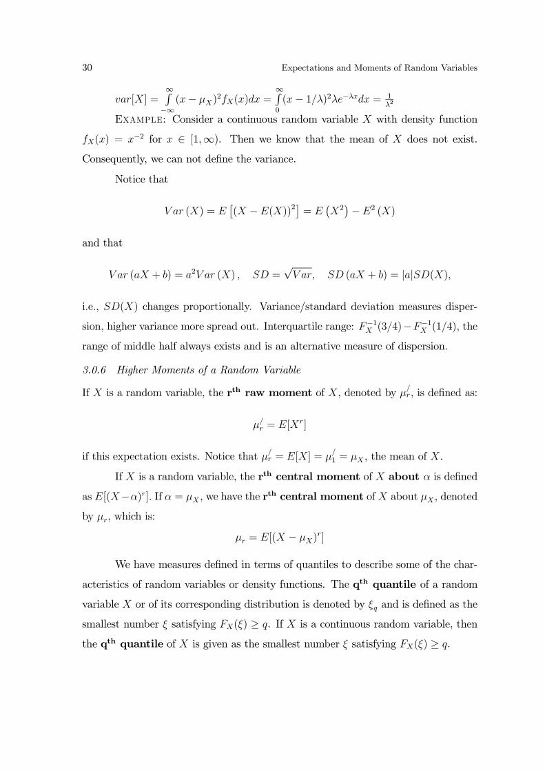
30 Expectations and Moments of Random Variables
var[X] =∞R−∞(x− μX)
2fX(x)dx =∞R0
(x− 1/λ)2λe−λxdx = 1λ2
Example: Consider a continuous random variable X with density function
fX(x) = x−2 for x ∈ [1,∞). Then we know that the mean of X does not exist.
Consequently, we can not define the variance.
Notice that
V ar (X) = E£(X −E(X))2
¤= E
¡X2¢−E2 (X)
and that
V ar (aX + b) = a2V ar (X) , SD =√V ar, SD (aX + b) = |a|SD(X),
i.e., SD(X) changes proportionally. Variance/standard deviation measures disper-
sion, higher variance more spread out. Interquartile range: F−1X (3/4)−F−1X (1/4), the
range of middle half always exists and is an alternative measure of dispersion.
3.0.6 Higher Moments of a Random Variable
If X is a random variable, the rth raw moment of X, denoted by μ/r, is defined as:
μ/r = E[Xr]
if this expectation exists. Notice that μ/r = E[X] = μ/1 = μX , the mean of X.
If X is a random variable, the rth central moment of X about α is defined
as E[(X−α)r]. If α = μX , we have the rth central moment of X about μX , denoted
by μr, which is:
μr = E[(X − μX)r]
We have measures defined in terms of quantiles to describe some of the char-
acteristics of random variables or density functions. The qth quantile of a random
variable X or of its corresponding distribution is denoted by ξq and is defined as the
smallest number ξ satisfying FX(ξ) ≥ q. If X is a continuous random variable, then
the qth quantile of X is given as the smallest number ξ satisfying FX(ξ) ≥ q.

Expectations and Moments of Random Variables 31
The median of a random variable X, denoted by medX or med(X), or ξq, is
the 0.5th quantile. Notice that if X a continuous random variable the median of X
satisfies:
Z med(X)
−∞fX(x)dx =
1
2=
Z ∞
med(X)
fX(x)dx
so the median of X is any number that has half the mass of X to its right and the
other half to its left. The median and the mean are measures of central location.
The third moment about the mean μ3 = E (X −E (X))3 is called a measure
of asymmetry, or skewness. Symmetrical distributions can be shown to have μ3 = 0.
Distributions can be skewed to the left or to the right. However, knowledge of the
third moment gives no clue as to the shape of the distribution, i.e. it could be the
case that μ3 = 0 but the distribution to be far from symmetrical. The ratio μ3σ3is
unitless and is call the coefficient of skewness. An alternative measure of skewness
is provided by the ratio: (mean-median)/(standard deviation)
The fourth moment about the mean μ4 = E (X −E (X))4 is used as a measure
of kurtosis, which is a degree of flatness of a density near the center. The coefficient
of kurtosis is defined as μ4σ4− 3 and positive values are sometimes used to indicate
that a density function is more peaked around its center than the normal (leptokur-
tic distributions). A positive value of the coefficient of kurtosis is indicative for a
distribution which is flatter around its center than the standard normal (platykurtic
distributions). This measure suffers from the same failing as the measure of skewness
i.e. it does not always measure what it supposed to.
While a particular moment or a few of the moments may give little information
about a distribution the entire set of moments will determine the distribution exactly.
In applied statistics the first two moments are of great importance, but the third and
forth are also useful.
32 Expectations and Moments of Random Variables
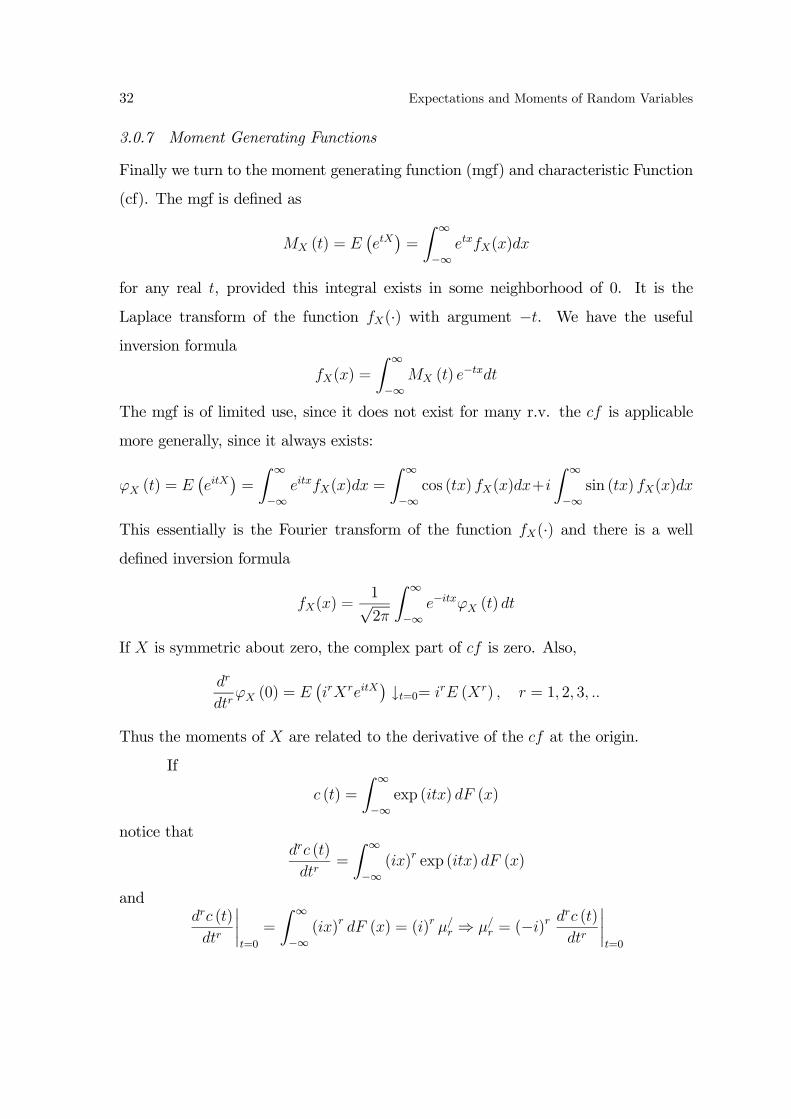
3.0.7 Moment Generating Functions
Finally we turn to the moment generating function (mgf) and characteristic Function
(cf). The mgf is defined as
MX (t) = E¡etX¢=
Z ∞
−∞etxfX(x)dx
for any real t, provided this integral exists in some neighborhood of 0. It is the
Laplace transform of the function fX(·) with argument −t. We have the useful
inversion formula
fX(x) =
Z ∞
−∞MX (t) e
−txdt
The mgf is of limited use, since it does not exist for many r.v. the cf is applicable
more generally, since it always exists:
ϕX (t) = E¡eitX
¢=
Z ∞
−∞eitxfX(x)dx =
Z ∞
−∞cos (tx) fX(x)dx+i
Z ∞
−∞sin (tx) fX(x)dx
This essentially is the Fourier transform of the function fX(·) and there is a well
defined inversion formula
fX(x) =1√2π
Z ∞
−∞e−itxϕX (t) dt
If X is symmetric about zero, the complex part of cf is zero. Also,
dr
dtrϕX (0) = E
¡irXreitX
¢↓t=0= irE (Xr) , r = 1, 2, 3, ..
Thus the moments of X are related to the derivative of the cf at the origin.
If
c (t) =
Z ∞
−∞exp (itx) dF (x)
notice thatdrc (t)
dtr=
Z ∞
−∞(ix)r exp (itx) dF (x)
anddrc (t)
dtr
¯t=0
=
Z ∞
−∞(ix)r dF (x) = (i)r μ/r ⇒ μ/r = (−i)
r drc (t)
dtr
¯t=0

Expectations and Moments of Random Variables 33
the rth uncenterd moment. Now expanding c (t) in powers of t we get
c (t) = c (0) +drc (t)
dtr
¯t=0
t+ ...+drc (t)
dtr
¯t=0
(t)r
r!+ ... = 1+ μ
/1 (it) + ...+ μ/r
(it)r
r!+ ...
The cummulants are defined as the coefficients κ1, κ2, ..., κr of the identity in it
exp
Ãκ1 (it) + κ2
(it)2
2!+ ...+ κr
(it)r
r!+ ...
!= 1 + μ
/1 (it) + ...+ μ/r
(it)r
r!+ ...
= c (t) =
Z ∞
−∞exp (itx) dF (x)
The cumulant-moment connection:
Suppose X is a random variable with n moments a1, ...an. Then X has n
cumulants k1, ...kn and
ar+1 =rX
j=0
⎛⎝ r
j
⎞⎠ ajkr+1−j for r = 0, ..., n− 1.
Writing out for r = 0, ...3 produces:
a1 = k1
a2 = k2 + a1k1
a3 = k3 + 2a1k2 + a2k1
a4 = k4 + 3a1k3 + 3a2k2 + a3k1.
These recursive formulas can be used to calculate the a0s efficiently from the
k0s, and vice versa. When X has mean 0, that is, when a1 = 0 = k1, aj becomes
μj = E((X −E(X))j),
so the above formulas simplify to:
μ2 = k2
μ3 = k3
μ4 = k4 + 3k22.

34 Expectations and Moments of Random Variables
3.0.8 Expectations of Functions of Random Variablers
Product and Quotient
Let f (X,Y ) = XY, E (X) = μX and E (Y ) = μY . Then, expanding f (X,Y ) = X
Y
around (μX , μY ), we have
f (X,Y ) =μXμY+1
μY(X − μX)−
μX(μY )
2 (Y − μY )+μX(μY )
3 (Y − μY )2− 1
(μY )2 (X − μX) (Y − μY )
as ∂f∂X
= 1Y, ∂f
∂Y= − X
Y 2, ∂2f
∂X2 = 0, ∂2f∂X∂Y
= ∂2f∂Y ∂X
= − 1Y 2, and ∂2f
∂Y 2= 2 X
Y 3. Taking
expectations we have
E
µX
Y
¶=
μXμY
+μX(μY )
3V ar (Y )−1
(μY )2Cov (X,Y ) .
For the variance, take again the variance of the Taylor expansion and keeping only
terms up to order 2 we have:
V ar
µX
Y
¶=(μX)
2
(μY )2
∙V ar (X)
(μX)2 +
V ar (Y )
(μY )2 − 2
Cov (X,Y )
μXμY
¸.

Chapter 4
EXAMPLES OF PARAMETRIC UNIVARIATE DISTRIBUTIONS
A parametric family of density functions is a collection of density functions that are
indexed by a quantity called parameter, e.g. let f(x;λ) = λe−λx for x > 0 and some
λ > 0. λ is the parameter, and as λ ranges over the positive numbers, the collection
f(.;λ) : λ > 0 is a parametric family of density functions.
4.0.9 Discrete Distributions
UNIFORM:
Suppose that for j = 1, 2, 3, ...., n
P (X = xj|X ) =1
n
where x1, x2, ...xn = X is the support. Then
E (X) =1
n
nXj=1
xj, V ar (X) =1
n
nXj=1
x2j −Ã1
n
nXj=1
xj
!2.
The c.d.f. here is
P (X ≤ x) =1
n
nXj=1
1 (xj ≤ x)
Bernoulli
A random variable whose outcome have been classified into two categories, called
“success” and “failure”, represented by the letters s and f, respectively, is called a
Bernoulli trial. If a random variable X is defined as 1 if a Bernoulli trial results in

36 Examples of Parametric Univariate Distributions
success and 0 if the same Bernoulli trial results in failure, then X has a Bernoulli
distribution with parameter p = P [success]. The definition of this distribution is:
A random variable X has a Bernoulli distribution if the discrete density of X
is given by:
fX(x) = fX(x; p) =
⎧⎨⎩ px(1− p)1−x for x = 0, 1
0 otherwise
where p = P [X = 1]. For the above defined random variable X we have that:
E[X] = p and var[X] = p(1− p)
BINOMIAL:
Consider a random experiment consisting of n repeated independent Bernoulli trials
with p the probability of success at each individual trial. Let the random variable X
represent the number of successes in the n repeated trials. ThenX follows a Binomial
distribution. The definition of this distribution is:
A random variable X has a binomial distribution, X ∼ Binomial(n, p), if
the discrete density of X is given by:
fX(x) = fX(x;n, p) =
⎧⎪⎪⎪⎨⎪⎪⎪⎩⎛⎝ n
x
⎞⎠ px(1− p)n−x for x = 0, 1, ..., n
0 otherwise
where p = P [X = 1] i.e. the probability of success in each independent Bernoulli
trial and n is the total number of trials. For the above defined random variable X
we have that:
E[X] = np and var[X] = np(1− p)
Mgf
MX (t) =£pet + (1− p)
¤n.
Example: Consider a stock with value S = 50. Each period the stock moves
up or down, independently, in discrete steps of 5. The probability of going up is

Examples of Parametric Univariate Distributions 37
p = 0.7 and down 1 − p = 0.3. What is the expected value and the variance of the
value of the stock after 3 period?
If we call X the random variable which is a success if the stock moves up
and failure if the stock moves down. Then P [X = success] = P [X = 1] = 0.7, and
X˜Binomial(3, p). Now X can take the values 0, 1, 2, 3 i.e. no success, 1 success and
2 failures, etc.. The value of the stock in each case and the probabilities are:
S = 35, and fX(0) =
⎛⎝ 3
0
⎞⎠ p0(1− p)3−0 = 1 ∗ 0.33 = 0.027,
S = 45, and fX(1) =
⎛⎝ 3
1
⎞⎠ p1(1− p)3−1 = 3 ∗ 0.7 ∗ 0.32 = 0.189,
S = 55, and fX(2) =
⎛⎝ 3
2
⎞⎠ p2(1− p)3−2 = 3 ∗ 0.72 ∗ 0.3 = 0.441,
S = 65 and fX(3) =
⎛⎝ 3
3
⎞⎠ p3(1− p)3−3 = 1 ∗ 0.73 = 0.343.
Hence the expected stock value is:
E[S] = 35 ∗ 0.027 + 45 ∗ 0.189 + 55 ∗ 0.441 + 65 ∗ 0.343 = 56, and var[S] =
(35− 56)2 ∗ 0.027 + (−11)2 ∗ 0.189 + (−1)2 ∗ 0.441 + (9)2 ∗ 0.343.
Hypergeometric
LetX denote the number of defective balls in a sample of size n when sampling is done
without replacement from a box containing M balls out of which K are defective.
The X has a hypergeometric distribution. The definition of this distribution is:
A random variable X has a hypergeometric distribution if the discrete den-
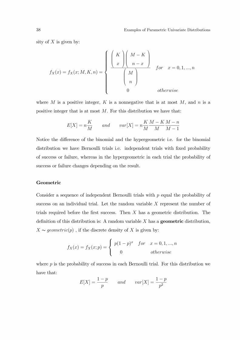
38 Examples of Parametric Univariate Distributions
sity of X is given by:
fX(x) = fX(x;M,K,n) =
⎧⎪⎪⎪⎪⎪⎪⎪⎪⎪⎨⎪⎪⎪⎪⎪⎪⎪⎪⎪⎩
⎛⎜⎜⎜⎝ K
x
⎞⎟⎟⎟⎠⎛⎜⎜⎜⎝ M −K
n− x
⎞⎟⎟⎟⎠⎛⎜⎜⎜⎝ M
n
⎞⎟⎟⎟⎠for x = 0, 1, ..., n
0 otherwise
where M is a positive integer, K is a nonnegative that is at most M , and n is a
positive integer that is at most M . For this distribution we have that:
E[X] = nK
Mand var[X] = n
K
M
M −K
M
M − n
M − 1
Notice the difference of the binomial and the hypergeometric i.e. for the binomial
distribution we have Bernoulli trials i.e. independent trials with fixed probability
of success or failure, whereas in the hypergeometric in each trial the probability of
success or failure changes depending on the result.
Geometric
Consider a sequence of independent Bernoulli trials with p equal the probability of
success on an individual trial. Let the random variable X represent the number of
trials required before the first success. Then X has a geometric distribution. The
definition of this distribution is: A random variable X has a geometric distribution,
X ∼ geometric(p) , if the discrete density of X is given by:
fX(x) = fX(x; p) =
⎧⎨⎩ p(1− p)x for x = 0, 1, ..., n
0 otherwise
where p is the probability of success in each Bernoulli trial. For this distribution we
have that:
E[X] =1− p
pand var[X] =
1− p
p2

Examples of Parametric Univariate Distributions 39
It is worth noticing that the Binomial distribution Binomial(n, p) can be
approximated by a Poisson(np) (see below). The approximation is more valid as
n→∞, p→ 0, in such a way so that np = constant.
POISSON:
A random variable X has a Poisson distribution, X ∼ Poisson(λ), if the discrete
density of X is given by:
P (X = x|λ) = e−λλx
x!x = 0, 1, 2, 3, ...
In calculations with the Poisson distribution we may use the fact that
et =∞Xj=0
tj
j!for any t.
Employing the above we can prove that
E (X) = λ, E (X (X − 1)) = λ2, V ar (X) = λ.
The Poisson distribution provides a realistic model for many random phenomena.
Since the values of a Poisson random variable are nonnegative integers, any random
phenomenon for which a count of some sort is of interest is a candidate for modeling
in assuming a Poisson distribution. Such a count might be the number of fatal traffic
accidents per week in a given place, the number of telephone calls per hour, arriving
in a switchboard of a company, the number of pieces of information arriving per hour,
etc.
Example: It is known that the average number of daily changes in excess
of 1%, for a specific stock Index, occurring in each six-month period is 5. What is
the probability of having one such a change within the next 6 months? What is the
probability of at least 3 changes within the same period?
We model the number of in excess of 1% changes, X, within the next 6 months
as a Poisson process. We know that E[X] = λ = 5. Hence fX(x) = e−λλx
x!= e−55x
x!,

40 Examples of Parametric Univariate Distributions
for x = 0, 1, 2, , ... Then P [X = 1] = fX(1) =e−551
1!= 0.0337. Also P [X ≥ 3] =
1− P [X < 3] =
= 1− P [X = 0]− P [X = 1]− P [X = 2] =
= 1− e−550
0!− e−551
1!− e−552
2!= 0.875.
We can approximate the Binomial with Poisson. The approximation is better
the smaller the p and the larger the n.
4.0.10 Continuous Distributions
UNIFORM ON [a, b].
A very simple distribution for a continuous random variable is the uniform distribu-
tion. Its density function is:
f (x|a, b) =
⎧⎨⎩ 1b−a if x ∈ [a, b]
0 otherwise,
and
F (x|a, b) =Z x
a
f (z|a, b) dz = x− a
b− a,
where −∞ < a < b < ∞. Then the random variable X is defined to be uniformly
distributed over the interval [a, b]. Now if X is uniformly distributed over [a, b] then
E (X) =a+ b
2, median =
a+ b
2, V ar (X) =
(b− a)2
12.
If X v U [a, b] =⇒ X − a v U [0, b− a] =⇒ X−ab−a v U [0, b− a]. Notice that if
a random variable is uniformly distributed over one of the following intervals [a, b),
(a, b], (a, b) the density function, expected value and variance does not change.
Exponential Distribution
If a random variable X has a density function given by:
fX(x) = fX(x;λ) = λe−λx for 0 ≤ x <∞

Examples of Parametric Univariate Distributions 41
where λ > 0 then X is defined to have an (negative) exponential distribution. Now
this random variable X we have
E[X] =1
λand var[X] =
1
λ2
Pareto-Levy or Stable Distributions
The stable distributions are a natural generalization of the normal in that, as their
name suggests, they are stable under addition, i.e. a sum of stable random variables
is also a random variable of the same type. However, nonnormal stable distributions
have more probability mass in the tail areas than the normal. In fact, the nonnormal
stable distributions are so fat-tailed that their variance and all higher moments are
infinite.
Closed form expressions for the density functions of stable random variables
are available for only the cases of normal and Cauchy.
If a random variable X has a density function given by:
fX(x) = fX(x; γ, δ) =1
π
γ
γ2 + (x− δ)2for −∞ < x <∞
where −∞ < δ <∞ and 0 < γ <∞, then X is defined to have a Cauchy distribu-
tion. Notice that for this random variable even the mean is infinite.
Normal or Gaussian:
We say that X v N [μ, σ2] then
f¡x|μ, σ2
¢=
1√2πσ2
e−(x−μ)22σ2 , −∞ < x <∞
E (X) = μ, V ar (X) = σ2.
The distribution is symmetric about μ, it is also unimodal and positive everywhere.
NoticeX − μ
σ= Z v N [0, 1]
is the standard normal distribution.

42 Examples of Parametric Univariate Distributions
Lognormal Distribution
Let X be a positive random variable, and let a new random variable Y be defined
as Y = logX. If Y has a normal distribution, then X is said to have a lognormal
distribution. The density function of a lognormal distribution is given by
fX(x;μ, σ2) =
1
x√2πσ2
e−(log x−μ)2
2σ2 for 0 < x <∞
where μ and σ2 are parameters such that −∞ < μ <∞ and σ2 > 0. We haven
E[X] = eμ+12σ2 and var[X] = e2μ+2σ
2 − e2μ+σ2
Notice that if X is lognormally distributed then
E[logX] = μ and var[logX] = σ2
Gamma-χ2
f (x|α, β) = 1
Γ (α)βαxα−1e−
xβ , 0 < x <∞, α, β > 0
α is shape parameter, β is a scale parameter. Here Γ (α) =R∞0
tα−1e−tdt is the
Gamma function, Γ (n) = n!. The χ2k is when α = k, and β = 1.
Notice that we can approximate the Poisson and Binomial functions by the
normal, in the sense that if a random variable X is distributed as Poisson with
parameter λ, then X−λ√λis distributed approximately as standard normal. On the
other hand if Y ∼ Binomial(n, p) then Y−np√np(1−p)
∼ N(0, 1).
The standard normal is an important distribution for another reason, as well.
Assume that we have a sample of n independent random variables, x1, x2, ..., xn, which
are coming from the same distribution with mean m and variance s2, then we have
the following:
1√n
nXi=1
xi −m
s∼ N(0, 1)
This is the well known Central Limit Theorem for independent observa-
tions.

Multivariate Random Variables 43
4.1 Multivariate Random Variables
We now consider the extension to multiple r.v., i.e.,
X = (X1,X2, ..,Xk) ∈ Rk
The joint pmf, fX(x), is a function with
P (X ∈ A) =Xx∈A
fX(x)
The joint pdf, fX(x), is a function with
P (X ∈ A) =
Zx∈A
fX(x)dx
This is a multivariate integral, and in general difficult to compute. If A is a rectangle
A = [a1, b1]× ...× [ak, bk], thenZx∈A
fX(x)dx =
bkZak
...
b1Za1
fX(x)dx1..dxk
The joint c.d.f. is defined similarly
FX (x) =X
z1≤x1,...,zk≤xk
fX(z1, z2, ..., zk)
FX (x) = P (X1 ≤ x1, ...,Xk ≤ xk) =
x1Z−∞
...
xnZ−∞
fX(z1, z2, ..., zk)dz1..dzk
The multivariate c.d.f. has similar coordinate-wise properties to a univariate c.d.f.
For continuously differentiable c.d.f.’s
fX(x) =∂kFX (x)
∂x1∂x2..∂xk
4.1.1 Conditional Distributions and Independence
We defined conditional probability P (A|B) = P (A∩B)/P (B) for events with P (B) 6=
0. We now want to define conditional distributions of Y |X. In the discrete case there
is no problem
fY |X(y|x) = P (Y = y|X = x) =f(y, x)
fX(x)

44 Examples of Parametric Univariate Distributions
when the event X = x has nonzero probability. Likewise we can define
FY |X(y|x) = P (Y ≤ y|X = x) =
PY≤y f(y, x)
fX(x)
Note that fY |X(y|x) is a density function and FY |X(y|x) is a c.d.f.
1) fY |X(y|x) ≥ 0 for all y
2)P
y fY |X(y|x) =P
y f(y,x)
fX(x)= fX(x)
fX(x)= 1
In the continuous case, it appears a bit anomalous to talk about the P (y ∈
A|X = x), since X = x itself has zero probability of occurring. Still, we define the
conditional density function
fY |X(y|x) =f(y, x)
fX(x)
in terms of the joint and marginal densities. It turns out that fY |X(y|x) has the
properties of p.d.f.
1) fY |X(y|x) ≥ 0
2)R∞−∞ fY |X(y|x)dy =
R∞−∞ f(y,x)dy
fX(x)= fX(x)
fX(x)= 1.
We can define Expectations within the conditional distribution
E(Y |X = x) =
Z ∞
−∞yfY |X(y|x)dy =
R∞−∞ yf(y, x)dyR∞−∞ f(y, x)dy
and higher moments of the conditional distribution
4.1.2 Independence
We say that Y and X are independent (denoted by ⊥⊥) if
P (Y ∈ A,X ∈ B) = P (Y ∈ A)P (X ∈ B)
for all events A, B, in the relevant sigma-algebras. This is equivalent to the cdf’s
version which is simpler to state and apply.
FY X(y, x) = F (y)F (x)

Multivariate Random Variables 45
In fact, we also work with the equivalent density version
f(y, x) = f(y)f(x) for all y, x
fY |X(y|x) = f(y) for all y
fX|Y (x|y) = f(x) for all x
If Y ⊥⊥ X, then g(X) ⊥⊥ h(Y ) for any measurable functions g, and h.
We can generalise the notion of independence to multiple random variables.
Thus Y , X, and Z are mutually independent if:
f(y, x, z) = f(y)f(x)f(z)
f(y, x) = f(y)f(x) for all y, x
f(x, z) = f(x)f(z) for all x, z
f(y, z) = f(y)f(z) for all y, z
for all y, x, z.
4.1.3 Examples of Multivariate Distributions
Multivariate Normal
We say that X (X1, X2, ...,Xk) vMVNk (μ,Σ) , when
fX (x|μ,Σ) =1
(2π)k/2 [det (Σ)]1/2exp
µ−12(x− μ)/Σ−1 (x− μ)
¶where Σ is a k × k covariance matrix
Σ =
⎛⎜⎜⎜⎜⎜⎜⎝σ11 σ12 ... σ1k
. . ....
. . ....
σkk
⎞⎟⎟⎟⎟⎟⎟⎠and det (Σ) is the determinant of Σ.

46 Examples of Parametric Univariate Distributions
Theorem 8 (a) If X v MVNk (μ,Σ) then Xi v N (μi, σii) (this is shown by inte-
gration of the joint density with respect to the other variables).
(b) The conditional distributions X = (X1, X2) are Normal too
fX1|X2 (x1|x2) v N¡μX1|X2
,ΣX1|X2
¢where
μX1|X2= μ1 + Σ12Σ
−122 (x2 − μ2) , ΣX1|X2 = Σ11 − Σ12Σ
−122 Σ21.
(c) Iff Σ diagonal then X1,X2, ..,Xk are mutually independent. In this case
det (Σ) = σ11σ22..σkk
−12(x− μ)/Σ−1 (x− μ) = −1
2
kXj=1
¡xj − μj
¢2σjj
so that
fX (x|μ,Σ) =kY
j=1
1p2πσjj
exp
Ã−12
¡xj − μj
¢2σjj
!4.1.4 More on Conditional Distributions
We now consider the relationship between two, or more, r.v. when they are not inde-
pendent. In this case, conditional density fY |X and c.d.f. FY |X is in general varying
with the conditioning point x. Likewise for conditional mean E (Y |X), conditional
medianM (Y |X), conditional variance V (Y |X), conditional cf E¡eitY |X
¢, and other
functionals, all of which characterize the relationship between Y and X. Note that
this is a directional concept, unlike covariance, and so for example E (Y |X) can be
very different from E (X|Y ).
Regression Models:
We start with random variable (Y,X). We can write for any such random variable
Y =
m(X)z | E (Y |X)| z
systematic part
+
εz | Y −E (Y |X)| z rand om part

Multivariate Random Variables 47
By construction ε satisfies E (ε|X) = 0, but ε is not necessarily independent of X.
For example, V ar (ε|X) = V ar (Y −E (Y |X) |X) = V ar (Y |X) = σ2 (X) can be
expected to vary with X as much as m (X) = E (Y |X) . A convenient and popular
simplification is to assume that
E (Y |X) = α+ βX
V ar (Y |X) = σ2
For example, in the bivariate normal distribution Y |X has
E (Y |X) = μY + ρY XσYσX
(X − μX)
V ar (Y |X) = σ2Y¡1− ρ2Y X
¢and in fact ε ⊥⊥ X.
We have the following result about conditional expectations
Theorem 9 (1) E (Y ) = E [E (Y |X)]
(2) E (Y |X) minimizes E£(Y − g (X))2
¤over all measurable functions g (·)
(3) V ar (Y ) = E [V ar (Y |X)] + V ar [E (Y |X)]
Proof. (1) Write fY X (y, x) = fY |X (y|x) fX (x) then we have E (Y ) =RyfY (y)dy =R
y¡R
fY X(y, x)dx¢dy =
Ry¡R
fY |X (y|x) fX (x) dx¢dy =
=R ¡R
yfY |X (y|x) dy¢fX (x) dx =
R[E(Y |X = x] fX (x) dx = E (E (Y |X))
(2) E£(Y − g (X))2
¤= E
£[Y − E (Y |X) +E (Y |X)− g (X)]2
¤= E [Y −E (Y |X)]2+2E [[Y − E (Y |X)] [E (Y |X)− g (X)]]+E [E (Y |X)− g (X)]2
as now E (Y E (Y |X)) = E£(E (Y |X))2
¤, and E (Y g (X)) = E (E (Y |X) g (X)) we
get thatE£(Y − g (X))2
¤= E [Y −E (Y |X)]2+E [E (Y |X)− g (X)]2 ≥ E [Y −E (Y |X)]2.
(3) V ar (Y ) = E [Y −E (Y )]2 = E [Y −E (Y |X)]2 +E [E (Y |X)−E (Y )]2
+2E [[Y −E (Y |X)] [E (Y |X)−E (Y )]]
The first term isE [Y −E (Y |X)]2 = EE£[Y − E (Y |X)]2 |X
¤ = E [V ar (Y |X)]
The second term is E [E (Y |X)−E (Y )]2 = V ar [E (Y |X)]
The third term is zero as ε = Y − E (Y |X) is such that E (ε|X) = 0, and
E (Y |X)−E (Y ) is measurable with respect to X.

48 Examples of Parametric Univariate Distributions
Covariance
Cov (X,Y ) = E [X −E (X)]E [Y −E (Y )] = E (XY )− E (X)E (Y )
Note that if X or Y is a constant then Cov (X,Y ) = 0. Also
Cov (aX + b, cY + d) = acCov (X,Y )
An alternative measure of association is given by the correlation coefficient
ρXY =Cov (X,Y )
σXσY
Note that
ρaX+b,cY+d = sign (a)× sign (c)× ρXY
If E (Y |X) = a = E (Y ) almost surely, then Cov (X,Y ) = 0. Also if X and Y are
independent r.v. then Cov (X,Y ) = 0.
Both the covariance and the correlation of random variables X and Y are
measures of a linear relationship of X and Y in the following sense. cov[X,Y ] will
be positive when (X − μX) and (Y − μY ) tend to have the same sign with high
probability, and cov[X,Y ] will be negative when (X−μX) and (Y −μY ) tend to have
opposite signs with high probability. The actual magnitude of the cov[X,Y ] does not
much meaning of how strong the linear relationship between X and Y is. This is
because the variability of X and Y is also important. The correlation coefficient does
not have this problem, as we divide the covariance by the product of the standard
deviations. Furthermore, the correlation is unitless and −1 ≤ ρ ≤ 1.
The properties are very useful for evaluating the expected return and stan-
dard deviation of a portfolio. Assume ra and rb are the returns on assets A and B,
and their variances are σ2a and σ2b , respectively. Assume that we form a portfolio of
the two assets with weights wa and wb, respectively. If the correlation of the returns
of these assets is ρ, find the expected return and standard deviation of the portfolio.
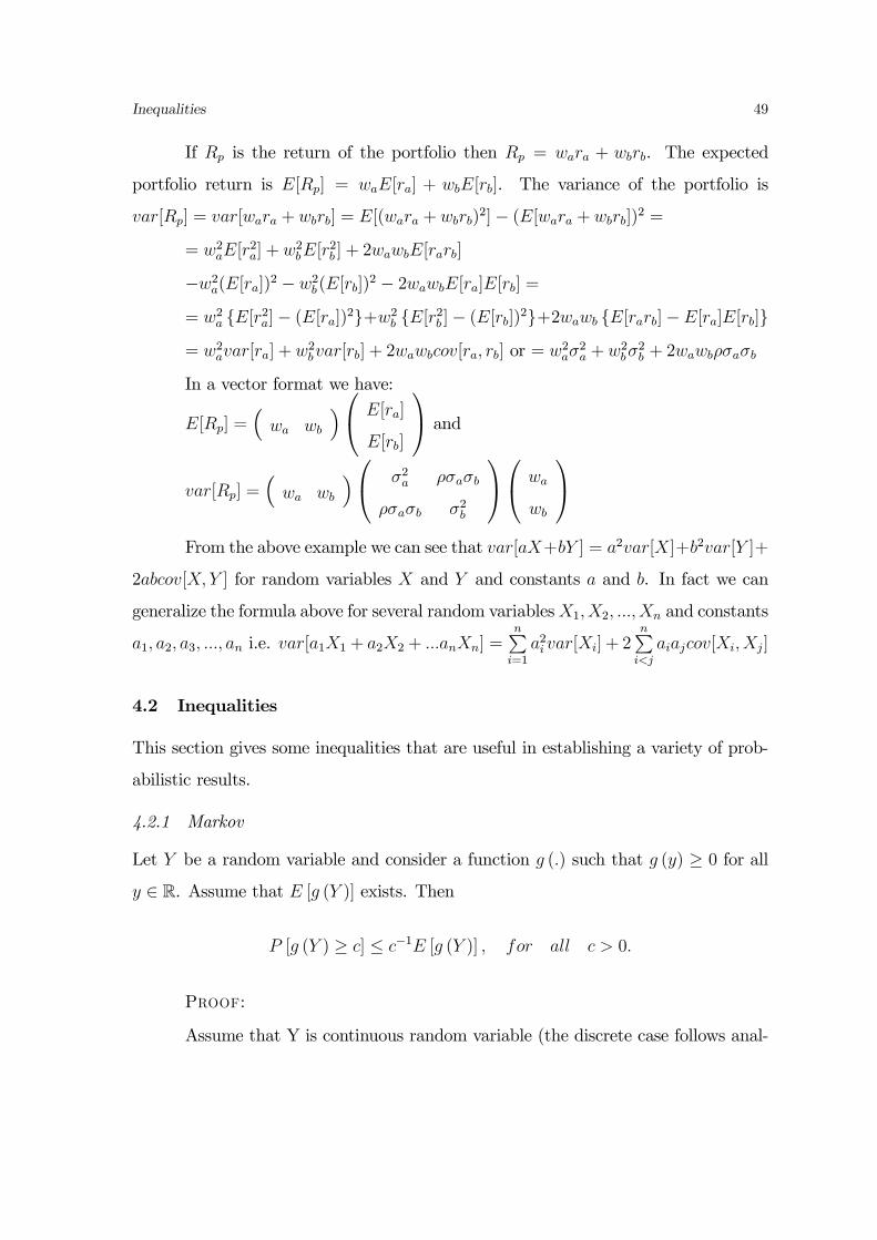
Inequalities 49
If Rp is the return of the portfolio then Rp = wara + wbrb. The expected
portfolio return is E[Rp] = waE[ra] + wbE[rb]. The variance of the portfolio is
var[Rp] = var[wara + wbrb] = E[(wara + wbrb)2]− (E[wara + wbrb])
2 =
= w2aE[r2a] + w2bE[r
2b ] + 2wawbE[rarb]
−w2a(E[ra])2 − w2b (E[rb])2 − 2wawbE[ra]E[rb] =
= w2a E[r2a]− (E[ra])2+w2b E[r2b ]− (E[rb])2+2wawb E[rarb]− E[ra]E[rb]
= w2avar[ra] + w2bvar[rb] + 2wawbcov[ra, rb] or = w2aσ2a + w2bσ
2b + 2wawbρσaσb
In a vector format we have:
E[Rp] =³wa wb
´⎛⎝ E[ra]
E[rb]
⎞⎠ and
var[Rp] =³wa wb
´⎛⎝ σ2a ρσaσb
ρσaσb σ2b
⎞⎠⎛⎝ wa
wb
⎞⎠From the above example we can see that var[aX+bY ] = a2var[X]+b2var[Y ]+
2abcov[X,Y ] for random variables X and Y and constants a and b. In fact we can
generalize the formula above for several random variablesX1,X2, ...,Xn and constants
a1, a2, a3, ..., an i.e. var[a1X1 + a2X2 + ...anXn] =nPi=1
a2i var[Xi] + 2nPi<j
aiajcov[Xi,Xj]
4.2 Inequalities
This section gives some inequalities that are useful in establishing a variety of prob-
abilistic results.
4.2.1 Markov
Let Y be a random variable and consider a function g (.) such that g (y) ≥ 0 for all
y ∈ R. Assume that E [g (Y )] exists. Then
P [g (Y ) ≥ c] ≤ c−1E [g (Y )] , for all c > 0.
Proof:
Assume that Y is continuous random variable (the discrete case follows anal-
50 Examples of Parametric Univariate Distributions
ogously) with p.d.f. f (.). Define A1 = y|g (y) ≥ c and A2 = y|g (y) < c. Then
E [g (Y )] =
ZA1
g (y) f (y) dy +
ZA2
g (y) f (y) dy
≥ZA1
g (y) f (y) dy ≥ZA1
cf (y) dy = cP [g (Y ) ≥ c] .
¥
4.2.2 Chebychev’s Inequality
P [|X − E (X)| ≥ η] ≤ V ar (X)
η2
or alternatively
Ph|X −E (X)| ≥ r
pV ar (X)
i≤ 1
r2
Proof:
To prove the above, assume that E (X) = 0 and compare 1 (|X| ≥ η) with X2
η2.
Clearly 1 (|X| ≥ η) ≤ X2
η2and it follows that E [1 (|X| ≥ η)] ≤ E(X2)
η2⇒ P [|X| ≥ η] ≤
V ar(X)η2
. Alternatively, apply Markov’s inequality by setting g (y) = [x−E (X)]2 and
c = r2V ar (X).¥
4.2.3 Minkowski
Let Y and Z be random variables such that [E (|Y |α)] < ∞ and [E (|Z|α)] < ∞ for
some 1 ≤ α <∞. Then
[E (|Y + Z|α)]1/α ≤ [E (|Y |α)]1/α + [E (|Z|α)]1/α
For α = 1 we have the triangular inequality
4.2.4 Triangle
E|X + Y | ≤ E|X|+E|Y |.
4.2.5 Cauchy-Schwarz
E2 (XY ) ≤ E (X)2E (Y )2
(P
ajbj)2 ≤
¡Pa2j¢ ¡P
b2j¢

Inequalities 51
Proof:
Let 0 ≤ h (t) = E£(tX − Y )2
¤= t2E (X2) + E (Y 2) − 2tE (XY ). Then the
function h (t) is a quadratic function in t which is increasing as t → ±∞. It has a
unique minimum at h/ (t) = 0 ⇒ 2tE (X2) − 2E (XY ) = 0 ⇒ t = E(XY )E(X2)
. Hence
0 ≤ h³E(XY )E(X2)
´⇒ E2 (XY ) ≤ E (X)2E (Y )2.¥
4.2.6 Hölder’s Inequality
For any p, q satisfying 1p+ 1
q= 1 we have
E |XY | ≤ (E |X|p)1p (E |Y |q)
1q
In fact the Cauchy-Schwarz inequality corresponds for p = q = 2.
4.2.7 Jensen Inequality
Let X be a random variable with mean E[X], and let g(.) be a convex function. Then
E[g(X)] ≥ g(E[X]).
Now a continuous function g(.) with domain and counterdomain the real line is called
convex if for any x0 on the real line, there exist a line which goes through the point
(x0, g(x0)) and lies on or under the graph of the function g(.). Also if g//(x0) ≥ 0
then g(.) is convex.

52 Examples of Parametric Univariate Distributions

Part II
Statistical Inference
53

Chapter 5
SAMPLING THEORY
To proceed we shall recall the following definitions.
Let X1,X2, ...,Xk be k random variables all defined on the same probability
space (Ω,A, P [.]). The joint cumulative distribution function of X1,X2, ..., Xk,
denoted by FX1,X2,...Xn(•, •, ..., •), is defined as
FX1,X2,...Xk(x1, x2, ..., xk) = P [X1 ≤ x1;X2 ≤ x2; ...;Xk ≤ xk]
for all (x1, x2, ..., xk).
Let X1,X2, ...,Xk be k discrete random variables, then the joint discrete
density function of these, denoted by fX1,X2,...Xk(•, •, ..., •), is defined to be
fX1,X2,...Xk(x1, x2, ..., xk) = P [X1 = x1;X2 = x2; ...;Xk = xk]
for (x1, x2, ..., xk), a value of (X1,X2, ..., Xk) and is 0 otherwise.
Let X1, X2, ..., Xk be k continuous random variables, then the joint contin-
uous density function of these, denoted by fX1,X2,...Xk(•, •, ..., •), is defined to be
a function such that
FX1,X2,...Xk(x1, x2, ..., xk) =
xkZ−∞
...
x1Z−∞
fX1,X2,...Xk(u1, u2, ..., uk)du1..duk
for all (x1, x2, ..., xk).
The totality of elements which are under discussion and about which infor-
mation is desired will be called the target population. The statistical problem is

56 Sampling Theory
to find out something about a certain target population. It is generally impossible
or impractical to examine the entire population, but one may examine a part of it
(a sample from it) and, on the basis of this limited investigation, make inferences
regarding the entire target population.
The problem immediately arises as to how the sample of the population should
be selected. Of practical importance is the case of a simple random sample, usually
called a random sample, which can be defined as follows:
Let the random variablesX1, X2, ..., Xn have a joint density fX1,X2,...Xn(x1, x2, ..., xn)
that factors as follows:
fX1,X2,...Xn(x1, x2, ..., xn) = f(x1)f(x2)...f(xn)
where f(.) is the common density of each Xi. Then X1, X2, ...,Xn is defined to be a
random sample of size n from a population with density f(.). Note that identical
distribution can be weakened - could have different population for each j - reflecting
heterogeneous individuals. Also, in time series we might want to allow dependence,
i.e., Xj and Xk are dependent. When we are dealing with finite population, sampling
without replacement causes some heterogeneity since ifX1 = x1, then the distribution
of X2 must be affected.
5.1 Sample Statistics
A sample statistic is a function of observable random variables, which is itself an
observable random variable, which does not contain any unknown parameters, i.e. a
sample statistic is any quantity we can write as a measurable function, T (X1, ...,Xn).
For example, let X1, X2, ...,Xk be a random sample from the density f(.). Then the
rth sample moment, denoted by M/r , is defined as:
M/r =
1
n
nXi=1
Xri .

Means and Variances 57
In particular, if r = 1, we get the sample mean, which is usually denoted by X orXn;
that is:
Xn =1
n
nXi=1
Xi
Also the rth sample central moment (about Xn), denoted byMr, is defined
as:
Mr =1
n
nXi=1
¡Xi −Xn
¢r.
In particular, if r = 2, we get the sample variance, and the sample standard deviation
s2 =1
n
nXi=1
¡Xi −X
¢2, s =
√s2
or maybe another sample statistic for the variance,
s2∗ =1
n− 1
nXi=1
¡Xi −X
¢2.
We can also get the sample Median,
M = median X1, ..., Xn =
⎧⎨⎩ X(r) if n = 2r − 112
£X(r) +X(r+1)
¤if n = 2r
the empirical cumulative distribution function
Fn(x) =1
n
nXi=1
1 (Xi ≤ x)
ϕn (t) =1
n
nXi=1
eitXi =1
n
nXi=1
sin (tXi) + i1
n
nXi=1
cos (tXi)
These are analogous of corresponding population characteristics and will be shown
to be similar to them when n is large. We calculate the properties of these variables:
(1) Exact properties; (2) Asymptotic.
5.2 Means and Variances
We can prove the following theorems:

58 Sampling Theory
Theorem 10 Let X1, X2, ...,Xk be a random sample from the density f(.). The
expected value of the rth sample moment is equal to the rth population moment, i.e.
the rth sample moment is an unbiased estimator of the rth population moment (Proof
omitted).
Theorem 11 Let X1, X2, ...,Xn be a random sample from a density f(.), and let
Xn =1n
nPi=1
Xi be the sample mean. Then
E[Xn] = μ and var[Xn] =1
nσ2
where μ and σ2 are the mean and variance of f(.), respectively. Notice that this is
true for any distribution f(.), provided that is not infinite.
Proof
E[Xn] = E[ 1n
nPi=1
Xi] =1n
nPi=1
E[Xi] =1n
nPi=1
μ = 1nnμ = μ. Also
var[Xn] = var[ 1n
nPi=1
Xi] =1n2
nPi=1
var[Xi] =1n2
nPi=1
σ2 = 1n2nσ2 = 1
nσ2
Theorem 12 Let X1,X2, ..., Xn be a random sample from a density f(.), and let s2∗
defined as above. Then
E[s2∗] = σ2 and var[s2∗] =1
n
µμ4 −
n− 3n− 1σ
4
¶where σ2 and μ4 are the variance and the 4
th central moment of f(.), respectively.
Notice that this is true for any distribution f(.), provided that μ4 is not infinite.
Proof
We shall prove first the following identity, which will be used latter:nPi=1
(Xi − μ)2 =nPi=1
¡Xi −Xn
¢2+ n
¡Xn − μ
¢2P(Xi − μ)2 =
P¡Xi −Xn +Xn − μ
¢2=P£¡
Xi −Xn
¢+¡Xn − μ
¢¤2=
=Ph¡
Xi −Xn
¢2+ 2
¡Xi −Xn
¢ ¡Xn − μ
¢+¡Xn − μ
¢2i=
=P¡
Xi −Xn
¢2+ 2
¡Xn − μ
¢P¡Xi −Xn
¢+ n
¡Xn − μ
¢2=

Sampling from the Normal Distribution 59
=P¡
Xi −Xn
¢2+ n
¡Xn − μ
¢2Using the above identity we obtain:
E[S2n] = E
∙1
n−1
nPi=1
(Xi −Xn)2
¸= 1
n−1E
∙nPi=1
(Xi − μ)2 − n¡Xn − μ
¢2¸=
= 1n−1
∙nPi=1
E (Xi − μ)2 − nE¡Xn − μ
¢2¸= 1
n−1
∙nPi=1
σ2 − nvar¡Xn
¢¸=
= 1n−1
£nσ2 − n 1
nσ2¤= σ2
The derivation of the variance of S2n is omitted.
Theorem 13 Let X1, ...,Xn be a random sample from a population with mean μ,
variance σ2, skewness κ3, and kurtosis κ4. Then,
(3) E (Fn(x)) = F (x), and V ar (Fn(x)) = F (x) (1− F (x)) /n
(4) Characteristic Function of X, ϕX (t) = [ϕX (t/n)]n.
Proof
E (Fn(x)) = E
µ1n
nPi=1
1 (Xi ≤ x)
¶= E (1 (Xi ≤ x)) = F (x) .Also V ar (Fn(x)) =
E [Fn(x)− F (x)]2 = E
½1n
nPi=1
1 [Xi ≤ x]− F (x)
¾2=
= E
(1n2
nPi=1
1 [Xi ≤ x]− F (x)2 + 1n2
nPi6=j1 [Xi ≤ x]− F (x) 1 [Xj ≤ x]− F (x)
)= 1
nE©1 [Xi ≤ x]− F (x)2
ª= 1
nE 1 [Xi ≤ x]− F 2 (x) = 1
nF 2 (x) [1− F (x)]
5.3 Sampling from the Normal Distribution
Theorem 14 Let denote Xn the sample mean of a random sample of size n from a
normal distribution with mean μ and variance σ2. Then (1) X v N(μ, σ2/n).
(2) X and s2 are independent.
(3) (n−1)s2∗σ2
v χ2n−1
(4) X−μs∗/√nv tn−1.
Proof

60 Sampling Theory
(1) From a Theorem above we have that
ϕX (t) = [ϕX (t/n)]n .
Now ϕX (t/n) = exp¡iμt− 1
2σ2t2
¢. Hence ϕX (t) =
hexp
³iμ t
n− 1
2σ2¡tn
¢2´in=
exp³iμt− 1
2
³σ2
n
´t2´, which is the cf of a normal distribution with mean μ and
variance σ2
n.
(2) For n = 2 we have that if X1 v N(0, 1) and X2 v N(0, 1) then X = X1+X2
2
and s2 = (X1−X2)2
4. Define Z1 =
X1+X2
2and Z2 =
X1−X2
2. Then Z1 and Z2 are
uncorrelated and by normality independent.
5.3.1 The Gamma Function
The gamma function is defined as:
Γ(t) =
∞Z0
xt−1e−xdx for t > 0
Notice that Γ(t+ 1) = tΓ(t),as
Γ(t+ 1) =
∞Z0
xte−xdx = −∞Z0
xtde−x = − xte−x¯∞0+ t
∞Z0
xt−1de−x = tΓ(t)
and if t is an integer then Γ(t+ 1) = t!. Also if t is again an integer then Γ(t+ 12) =
1∗3∗5∗...(2t−1)2t
√π. Finally Γ(1
2) =√π.
Recall that if X is a random variable with density
fX(x) =1
Γ(k/2)
µ1
2
¶k/2
xk2−1e−
12x for 0 < x <∞
where Γ(.) is the gamma function, then X is defined to have a chi-square distrib-
ution with k degrees of freedom.
Notice that X is distributed as above then:
E[X] = k and var[X] = 2k
We can prove the following theorem

Sampling from the Normal Distribution 61
Theorem 15 If the random variables Xi, i = 1, 2, .., k are normally and indepen-
dently distributed with means μi and variances σ2i then
U =kXi=1
µXi − μi
σi
¶2has a chi-square distribution with k degrees of freedom. Proof omitted.
Furthermore,
Theorem 16 If the random variables Xi, i = 1, 2, .., k are normally and indepen-
dently distributed with mean μ and variance σ2, and let S2 = 1n−1
nPi=1
(Xi − Xn)2
then
U =(n− 1)S2
σ2v χ2n−1
where χ2n−1 is the chi-square distribution with n−1 degrees of freedom. Proof omitted.
5.3.2 The F Distribution
If X is a random variable with density
fX(x) =Γ[(m+ n)/2]
Γ(m/2)Γ(n/2)
³mn
´m/2 xm2−1
[1 + (m/n)x](m+n)/2for 0 < x <∞
where Γ(.) is the gamma function, then X is defined to have a F distribution with
m and n degrees of freedom.
Notice that if X is distributed as above then:
E[X] =n
n− 2 and var[X] =2n2(m+ n− 2)m(n− 2)2(n− 4)
Theorem 17 If the random variables U and V are independently distributed as chi-
square with m and n degrees of freedom, respectively i.e. U v χ2m and V v χ2n
independently, thenU/m
V/n= X v Fm,n
where Fm,n is the F distribution with m,n degrees of freedom. Proof omitted.

62 Sampling Theory
5.3.3 The Student-t Distribution
If X is a random variable with density
fX(x) =Γ[(k + 1)/2]
Γ(k/2)
1√kπ
1
[1 + x2/k](k+1)/2for −∞ < x <∞
where Γ(.) is the gamma function, then X is defined to have a t distribution with
k degrees of freedom.
Notice that if X is distributed as above then:
E[X] = 0 and var[X] =k
k − 2
Theorem 18 If the random variables Z and V are independently distributed as stan-
dard normal and chi-square with k, respectively i.e. Z v (N(0, 1) and V v χ2k inde-
pendently, thenZpV/k
= X v tk
where tk is the t distribution with k degrees of freedom. Proof omitted.
The above Theorems are very useful especially to get the distribution of various
tests and construct confidence intervals.

Chapter 6
POINT AND INTERVAL ESTIMATION
The problem of estimation is defined as follows. Assume that some characteristic of
the elements in a population can be represented by a random variable X whose den-
sity is fX(.; θ) = f(.; θ), where the form of the density is assumed known except that
it contains an unknown parameter θ (if θ were known, the density function would
be completely specified, and there would be no need to make inferences about it.
Further assume that the values x1, x2, ..., xn of a random sample X1,X2, ...., Xn from
f(.; θ) can be observed. On the basis of the observed sample values x1, x2, ..., xn it
is desired to estimate the value of the unknown parameter θ or the value of some
function, say τ(θ), of the unknown parameter. The estimation can be made in two
ways. The first, called point estimation, is to let the value of some statistic, say
t(X1,X2, ....,Xn), represent or estimate, the unknown τ(θ). Such a statistic is called
the point estimator. The second, called interval estimation, is to define two
statistics, say t1(X1,X2, ...., Xn) and t2(X1,X2, ...., Xn), where t1(X1,X2, ....,Xn) <
t2(X1, X2, ....,Xn), so that (t1(X1, X2, ....,Xn), t2(X1, X2, ....,Xn)) constitutes an in-
terval for which the probability can be determined that it contains the unknown
τ(θ).
6.1 Parametric Point Estimation
The point estimation admits two problems. The first is to devise some means of ob-
taining a statistic to use as an estimator. The second, to select criteria and techniques

64 Point and Interval Estimation
to define and find a “best” estimator among many possible estimators.
6.1.1 Methods of Finding Estimators
Any statistic (known function of observable random variables that is itself a random
variable) whose values are used to estimate τ(θ), where τ(.) is some function of the
parameter θ, is defined to be an estimator of τ(θ).
Notice that for specific values of the realized random sample the estimator
takes a specific value called estimate.
6.1.2 Method of Moments
Let f(.; θ1, θ2, ..., θk) be a density of a random variable X which has k parameters
θ1, θ2, ..., θk. As before let μ/r denote the rth moment i.e. = E[Xr]. In general μ/r
will be a known function of the k parameters θ1, θ2, ..., θk. Denote this by writ-
ing μ/r = μ
/r(θ1, θ2, ..., θk). Let X1,X2, ...,Xn be a random sample from the density
f(.; θ1, θ2, ..., θk), and, as before, letM/j be the j
th sample moment, i.e. M/j =
1n
nPi=1
Xji .
Then equating sample moments to population ones we get k equations with k un-
knowns, i.e.
M/j = μ
/j(θ1, θ2, ..., θk) for j = 1, 2, ..., k
Let the solution to these equations be bθ1,bθ2, ...,bθk. We say that these k estimatorsare the estimators of θ1, θ2, ..., θk obtained by the method of moments.
Example: Let X1, X2, ...,Xn be a random sample from a normal distribution
with mean μ and variance σ2. Let (θ1, θ2) = (μ, σ2). Estimate the parameters μ and
σ by the method of moments.. Recall that σ2 = μ/2− (μ
/1)2 and μ = μ
/1. The method
of moment equations become:
1n
nPi=1
Xi = X =M/1 = μ
/1 = μ
/1(μ, σ
2) = μ
1n
nPi=1
X2i =M
/2 = μ
/2 = μ
/2(μ, σ
2) = σ2 + μ2
Solving the two equations for μ and σ we get:bμ = X, and bσ =r 1n
nPi=1
(Xi −X) which are the M-M estimators of μ and σ.

Parametric Point Estimation 65
Example: Let X1,X2, ...,Xn be a random sample from a Poisson distribution
with parameter λ. There is only one parameter, hence only one equation, which is:
1n
nPi=1
Xi = X =M/1 = μ
/1 = μ
/1(λ) = λ
Hence the M-M estimator of λ is bλ = X.
6.1.3 Maximum Likelihood
Consider the following estimation problem. Suppose that a box contains a number of
black and a number of white balls, and suppose that it is known that the ratio of the
number is 3/1 but it is not known whether the black or the white are more numerous,
i.e. the number of drawing a black ball is either 1/4 or 3/4. If n balls are drawn with
replacement from the box, the distribution of X, the number of black balls, is given
by the binomial distribution
f(x; p) =
⎛⎝ n
x
⎞⎠ px(1− p)n−x for x = 0, 1, 2, ..., n
where p is the probability of drawing a black ball. Here p = 1/4 or p = 3/4. We shall
draw a sample of three balls, i.e. n = 3, with replacement and attempt to estimate
the unknown parameter p of the distribution. the estimation is simple in this case as
we have to choose only between the two numbers 1/4 = 0.25 and 3/4 = 0.75. The
possible outcomes and their probabilities are given below:
outcome : x 0 1 2 3
f(x; 0.75) 1/64 9/64 27/64 27/64
f(x; 0.25) 27/64 27/64 9/64 1/64
In the present example, if we found x = 0 in a sample of 3, the estimate 0.25
for p would be preferred over 0.75 because the probability 27/64 is greater than 1/64,
i.e.

66 Point and Interval Estimation
And in general we should estimate p by 0.25 when x = 0 or 1 and by 0.75
when x = 2 or 3. The estimator may be defined as
bp = bp(x) =⎧⎨⎩ 0.25 for x = 0, 1
0.75 for x = 2, 3
The estimator thus selects fro every possible x the value of p, say bp, such thatf(x; bp) > f(x; p/)
where p/ is the other value of p.
More generally, if several values of p were possible, we might reasonably pro-
ceed in the same manner. Thus if we found x = 2 in a sample of 3 from a binomial
population, we should substitute all possible values of p in the expression
f(2; p) =
⎛⎝ 3
2
⎞⎠ p2(1− p) for 0 ≤ p ≤ 1
and choose as our estimate that value of p which maximizes f(2; p). The position
of the maximum of the function above is found by setting equal to zero the first
derivative with respect to p, i.e. ddpf(2; p) = 6p − 9p2 = 3p(2 − 3p) = 0 ⇒ p = 0 or
p = 2/3. The second derivative is: d2
dp2f(2; p) = 6 − 18p. Hence, d2
dp2f(2; 0) = 6 and
the value of p = 0 represents a minimum, whereas d2
dp2f(2; 2
3) = −6 and consequently
p = 23represents the maximum. Hence bp = 2
3is our estimate which has the property
f(x; bp) > f(x; p/)
where p/ is any other value in the interval 0 ≤ p ≤ 1.
The likelihood function of n random variables X1,X2, ...,Xn is defined to
be the joint density of the n random variables, say fX1,X2,...,Xn(x1, x2, ..., xn; θ), which
is considered to be a function of θ. In particular, if X1,X2, ...,Xn is a random sample
from the density f(x; θ), then the likelihood function is f(x1; θ)f(x2; θ).....f(xn; θ).
To think of the likelihood function as a function of θ, we shall use the notation
L(θ;x1, x2, ..., xn) or L(•;x1, x2, ..., xn) for the likelihood function in general.

Parametric Point Estimation 67
The likelihood is a value of a density function. Consequently, for discrete
random variables it is a probability. Suppose for the moment that θ is known, denoted
by θ0. The particular value of the random variables which is “most likely to occur”
is that value x/1, x/2, ..., x
/n such that fX1,X2,...,Xn(x1, x2, ..., xn; θ0) is a maximum. for
example, for simplicity let us assume that n = 1 and X1 has the normal density
with mean 0 and variance 1. Then the value of the random variable which is most
likely to occur is X1 = 0. By “most likely to occur” we mean the value x/1 of X1
such that φ0,1(x/1) > φ0,1(x1). Now let us suppose that the joint density of n random
variables is fX1,X2,...,Xn(x1, x2, ..., xn; θ), where θ is known. Let the particular values
which are observed be represented by x/1, x
/2, ..., x
/n. We want to know from which
density is this particular set of values most likely to have come. We want to know
from which density (what value of θ) is the likelihood largest that the set x/1, x/2, ..., x
/n
was obtained. in other words, we want to find the value of θ in the admissible set,
denoted by bθ, which maximizes the likelihood function L(θ;x/1, x
/2, ..., x
/n). The valuebθ which maximizes the likelihood function is, in general, a function of x1, x2, ..., xn,
say bθ = bθ(x1, x2, ..., xn). Hence we have the following definition:Let L(θ) = L(θ;x1, x2, ..., xn) be the likelihood function for the random vari-
ables X1,X2, ...,Xn. If bθ [where bθ = bθ(x1, x2, ..., xn) is a function of the observationsx1, x2, ..., xn] is the value of θ in the admissible range which maximizes L(θ), then bΘ =bθ(X1, X2, ...,Xn) is the maximum likelihood estimator of θ. bθ = bθ(x1, x2, ..., xn)is the maximum likelihood estimate of θ for the sample x1, x2, ..., xn.
The most important cases which we shall consider are those in whichX1,X2, ...,Xn
is a random sample from some density function f(x; θ), so that the likelihood function
is
L(θ) = f(x1; θ)f(x2; θ).....f(xn; θ)
Many likelihood functions satisfy regularity conditions so the maximum likelihood
estimator is the solution of the equation
dL(θ)
dθ= 0

68 Point and Interval Estimation
Also L(θ) and logL(θ) have their maxima at the same value of θ, and it is sometimes
easier to find the maximum of the logarithm of the likelihood. Notice also that if
the likelihood function contains k parameters then we find the estimator from the
solution of the k first order conditions.
Example: Let a random sample of size n is drawn from the Bernoulli distri-
bution
f(x; p) = px(1− p)1−x
where 0 ≤ p ≤ 1. The sample values x1, x2, ..., xn will be a sequence of 0s and 1s, and
the likelihood function is
L(p) =nYi=1
pxi(1− p)1−xi = pP
xi(1− p)n−P
xi
Let y =P
xi we obtain that
logL(p) = y log p+ (n− y) log(1− p)
andd logL(p)
dp=
y
p− n− y
1− p
Setting this expression equal to zero we get
bp = y
n=1
n
Xxi = x
which is intuitively what the estimate for this parameter should be.
Example: Let a random sample of size n is drawn from the normal distrib-
ution with density
f(x;μ, σ2) =1√2πσ2
e−(x−μ)22σ2
The likelihood function is
L(μ, σ2) =nYi=1
1√2πσ2
e−(xi−μ)
2
2σ2 =
µ1
2πσ2
¶n/2
exp
"− 1
2σ2
nXi=1
(xi − μ)2
#

Interval Estimation 69
the logarithm of the likelihood function is
logL(μ, σ2) = −n2log 2π − n
2log σ2 − 1
2σ2
nXi=1
(xi − μ)2
To find the maximum with respect to μ and σ2 we compute
∂ logL
∂μ=1
σ2
nXi=1
(xi − μ)
and∂ logL
∂σ2= −n
2
1
σ2+
1
2σ4
nXi=1
(xi − μ)2
and putting these derivatives equal to 0 and solving the resulting equations we find
the estimates bμ = 1
n
nXi=1
xi = x
and bσ2 = 1
n
nXi=1
(xi − x)2
which turn out to be the sample moments corresponding to μ and σ2.
6.1.4 Properties of Point Estimators
One needs to define criteria so that various estimators can be compared. One of these
is the unbiasedness. An estimator T = t(X1,X2, ...,Xn) is defined to be an unbiased
estimator of τ(θ) if and only if
Eθ[T ] = Eθ[t(X1,X2, ..., Xn)] = τ(θ)
for all θ in the admissible space.
Other criteria are consistency, mean square error etc.
6.2 Interval Estimation
In practice estimates are often given in the form of the estimate plus or minus a
certain amount e.g. the cost per volume of a book could be 83± 4.5 per cent which

70 Point and Interval Estimation
means that the actual cost will lie somewhere between 78.5% and 87.5% with high
probability. Let us consider a particular example. Suppose that a random sample
(1.2, 3.4, .6, 5.6) of four observations is drawn from a normal population with unknown
mean μ and a known variance 9. The maximum likelihood estimate of μ is the sample
mean of the observations:
x = 2.7
We wish to determine upper and lower limits which are rather certain to
contain the true unknown parameter value between them. We know that the sample
mean, x, is distributed as normal with mean μ and variance 9/n i.e. x v N(μ, σ2/n).
Hence we have
Z =X − μ
32
v N(0, 1)
Hence Z is standard normal. Consequently we can find the probability that Z will
be between two arbitrary values. For example we have that
P [−1.96 < Z < 1.96] =
1.96Z−1.96
φ(z)dz = 0.95
Hence we get that μ must be in the interval
X +3
21.96 > μ > X − 3
21.96
and for the specific value of the sample mean we have that 5.64 > μ > −.24 i.e.
P [5.64 > μ > −.24] = .95. This leads us to the following definition for the confidence
interval.
Let X1,X2, ....,Xn be a random sample from the density f(•; θ). Let T1 =
t1(X1, X2, ....,Xn) and T2 = t2(X1, X2, ....,Xn) be two statistics satisfying T1 ≤ T2
for which Pθ[T1 < τ(θ) < T2] = γ, where γ does not depend on θ. Then the random
interval (T1, T2) is called a 100γ percent confidence interval for τ(θ). γ is called
the confidence coefficient. T1 and T2 are called the lower and upper confidence
limits, respectively. A value (t1, t2) of the random interval (T1, T2) is also called a
100γ percent confidence interval for τ(θ).

Interval Estimation 71
Let X1,X2, ....,Xn be a random sample from the density f(•; θ). Let T1 =
t1(X1, X2, ....,Xn) be a statistic for which Pθ[T1 < τ(θ)] = γ. Then T1 is called a one-
sided lower confidence interval for τ(θ). Similarly, let T2 = t2(X1,X2, ....,Xn)
be a statistic for which Pθ[τ(θ) < T2] = γ. Then T2 is called a one-sided upper
confidence interval for τ(θ).
Example: Let X1, X2, ....,Xn be a random sample from the density f(x; θ) =
φθ,9(x). Set T1 = t1(X1,X2, ...., Xn) = X − 6/√n and T2 = t2(X1, X2, ....,Xn) =
X + 6/√n. Then (T1, T2) constitutes a random interval and is a confidence interval
for τ(θ) = θ, with confidence coefficient γ = P [X − 6/√n < θ < X + 6/√n] =
= P [−2 < X−θ3√n
< 2] = Φ(2)−Φ(−2) = 0.9772− 0.0228 = 0.9544. hence if the
random sample of 25 observations has a sample mean of, say, 17.5, then the interval
(17.5− 6/√25, 17.5 + 6/
√25) is also called a confidence interval of θ.
6.2.1 Sampling from the Normal Distribution
Let X1,X2, ...,Xn be a random sample from the normal distribution with mean μ
and variance σ2. If σ2 is unknown then θ = (μ, σ2), the unknown parameters and
τ(θ) = μ, the parameter we want to estimate by interval estimation. We know that
X − μσ√n
v N(0, 1)
However, the problem with this statistic is that we have two parameters. Conse-
quently we can not an interval. hence we look for a statistic that involves only the
parameter we want to estimate, i.e. μ. Notice that
(X − μ)/ σ√nqP
(Xi −X)2/(n− 1)σ2=
X − μ
S/√nv tn−1
This statistic involves only the parameter we want to estimate. Hence we have½q1 <
X − μ
S/√n< q2
¾⇔©X − q2(S/
√n) < μ < X − q1(S/
√n)ª
where q1, q2 are such that
P
∙q1 <
X − μ
S/√n< q2
¸= γ

72 Point and Interval Estimation
Hence the interval¡X − q2(S/
√n),X − q1(S/
√n)¢is the 100γ percent confidence
interval for μ. It can be proved that if q1, q2 are symmetrical around 0, then the
length is the interval is minimized.
Alternatively, if we want to find a confidence interval for σ2, when μ is un-
known, then we use the statisticP(Xi −X)2
σ2=(n− 1)S2
σ2v χ2n−1
Hence we have½q1 <
(n− 1)S2σ2
< q2
¾⇔½(n− 1)S2
q2< σ2 <
(n− 1)S2q1
¾where q1, q2 are such that
P
∙q1 <
(n− 1)S2σ2
< q2
¸= γ
So the interval³(n−1)S2
q2, (n−1)S
2
q1
´is a 100γ percent confidence interval for σ2. The q1,
q2 are often selected so that Phq2 <
(n−1)S2σ2
i= P
h(n−1)S2
σ2< q1
i= (1− γ)/2. Such a
confidence interval is referred to as equal-tailed confidence interval for σ2.

Chapter 7
HYPOTHESIS TESTING
A statistical hypothesis is an assertion or conjecture, denoted by H, about a
distribution of one or more random variables. If the statistical hypothesis completely
specifies the distribution is simple, otherwise is composite.
Example Let X1, X2, ...,Xn be a random sample from f(x; θ) = φμ,25(x).
The statistical hypothesis that the mean of the normal population is less or equal
to 17 is denoted by: H : θ ≤ 17. Such a hypothesis is composite, as it does not
completely specify the distribution. On the other hand, the hypothesis H : θ ≤ 17 is
simple since it completely specifies the distribution.
A test of statistical hypothesis H is a rule or procedure for deciding whether
to reject H.
Example Let X1, X2, ...,Xn be a random sample from f(x; θ) = φμ,25(x).
Consider H : θ ≤ 17. One possible test Y is as follows: Reject H if and only if
X > 17 + 5/√n.
In many hypotheses-testing problems two hypotheses are discussed. The first,
the hypothesis being testing, is called the null hypothesis, denoted by H0, and the
second is called the alternative hypothesis denoted by H1. We say that H0 is
tested against or versus H1. The thinking is that if the null hypothesis is wrong the
alternative hypothesis is true, and vice versa. We can make two types of errors:
Rejection of H0 when H0 is true is called a Type I error, and acceptance of
H0 when H0 is false is called a Type II error. The size of Type I error is defined

74 Hypothesis testing
to be the probability that a Type I error is made, and similarly the size of a Type
II error is defined to be the probability that a Type II error is made.
Significance level or size of a test, denoted by α, is the supremum of the
probability of rejecting H0 when H0 is correct, i.e. it is the supremum of the Type I
error. In general to perform a test we fix the size to a prespecified value in general
10%, 5% or 1%.
Example Let X1, X2, ...,Xn be a random sample from f(x; θ) = φμ,25(x).
Consider H0 : θ ≤ 17 and the test Y: Reject H0 if and only if X > 17+ 5/√n. Then
of the test is
supθ≤17
P [X > 17 + 5/√n] = sup
θ≤17
PhX−θ5/√n> 17+5/
√n−θ
5/√n
i=
= supθ≤17
n1− P
hX−θ5/√n≤ 17+5/
√n−θ
5/√n
io= sup
θ≤17
n1− P
hZ ≤ 17+5/
√n−θ
5/√n
io=
= supθ≤17
n1− Φ
h17+5/
√n−θ
5/√n
io= 1− Φ(1) = 0.159
7.1 Testing Procedure
Let us establish a test procedure via an example. Assume that n = 64, X = 9.8 and
σ2 = 0.04. We would like to test the hypothesis that μ = 10.
1. Formulate the null hypothesis:
H0 : μ = 10
2. Formulate the alternative:
H1 : μ 6= 10
3. select the level of significance:
α = 0.01
From tables find the critical values for Z, denoted by cZ = 2.58.
4. Establish the rejection limits:
Reject H0 if Z < −2.58 or Z > 2.58.
5. Calculate Z:
Z = X−μ0σ√n
= 9.8−100.2/
√64= −8
6. Make the decision:

Testing Proportions 75
Since Z is less than −2.58, reject H0.
To find the appropriate test for the mean we have to consider the following
cases:
1. Normal population and known population variance (or standard deviation).
In this case the statistic we use is:
Z =X − μ0
σ√n
v N(0, 1)
2. Large samples in order to use the central limit theorem.
In this case the statistic we use is:
Z =X − μ0
S√n
v N(0, 1)
3. Small samples from a normal population where the population variance (or
standard deviation) is unknown.
In this case the statistic we use is:
t =X − μ0
S√n
v tn−1
7.2 Testing Proportions
The null hypothesis will be of the form:
H0 : π = π0
an the three possible alternatives are:
(1) H1 : π 6= π0 two sided test, (2) H1 : π < π0 one sided, (3) H1 : π > π0 one
sided. The appropriate statistic is based on the central limit theorem and is:
Z =p− π0
S√n
v N(0, 1) where S2 = π0(1− π0)
Example: Mr. X believes that he will get more 60% of the votes. However,in a sample of 400 voters 252 indicate that they will vote for X. At a significance level
of 5% test Mr. X belief.

76 Hypothesis testing
p = 252400= 0.63, S2 = 0.6(1− 0.6) = 0.24. The H0 : π = π0 and the alternative
is H1 : π > π0. The critical value is 1.64. Now Z = p−π0S√n
= 0.63−0.60.489/
√400
= 1.22.
Consequently, the null is not rejected as Z < 1.64. Thus Mr. X belief is wrong.
If fact we have the following possible outcomes when testing hypotheses:
H0 is accepted H1 is accepted
H0 is correct Correct decision (1− α) Type I error (α)
H1 is correct Type II error (β) Correct decision (1− β)
An operating characteristic curve presents the probability of accepting a
null hypothesis for various values of the population parameter at a given significance
level α using a particular sample size. The power of the test is the inverse function
of the operating characteristic curve, i.e. it is the probability of rejecting the null
hypothesis for various possible values of the population parameter.

Part III
Asymptotic Theory
77


Chapter 8
MODES OF CONVERGENCE
We have a statistic T which is a measurable function of the data
Tn = T (X1, ...,Xn) ,
and we would like to know what happens to Tn as n→∞. It turns out that the limit
is easier to work with than Tn itself. The plan is to use the limit as approximation
device. We think of a sequence T1, T2, ... which have distribution functions F1, F2, ....
Definition A sequence of random variables T1, T2, ... converges in probability
to a random variable T (denoted by Tnp−→ T ) if, for every ε > 0,
limn→∞
P [|Tn − T | > ε] = 0.
DefinitionA sequence of random variables T1, T2, ... converges in mean square
to a random variable T (denoted by Tnms−→ T ) if,
limn→∞
E (Tn − T )2 = 0
which is equivalent to (a) V ar (Tn) → 0 and (b) E (Tn)− E (T ) → 0 because of the
triangle inequality.
Theorem 19 Convergence in mean square implies convergence in probability.
Proof. By the Markov/Chebychev inequality,
P [|Tn − T | ≥ ε] ≤ E |Tn − T |2
ε2→ 0.

80 Modes of Convergence
Note that if Tn > 0,
P [Tn ≥ ε] ≤ E (Tn)2
ε2≤ E (Tn)
ε
so that if E(Tn)ε→ 0, this is sufficient for Tn
p−→ 0.
But the converse of the theorem is not necessarily true. To see this consider
the following random variable
Tn =
⎧⎨⎩ n with probability 1n
0 with probability 1− 1n
, T = 0.
Then P [Tn ≥ ε] = 1nfor any ε > 0, and P [Tn ≥ ε] = 1
n→ 0. But E (Tn)
2 = n2 1n=
n→∞.
A famous consequence of the theorem is the (Weak) Law of Large Numbers
Theorem 20 WEAK LAW of LARGE NUMBERS Let X1, ..., Xn be i.i.d. with
E (Xi) = μ and V ar (Xi) = σ2 <∞, and Tn = X. Then for all ε > 0,
limn→∞
P [|Tn − μ| > ε] = 0, i.e., Tnp−→ μ.
The proof is easy because
E[(Tn − μ)2] =σ2
n→ 0.
as we have shown. In fact, the result can be proved with only the hypothesis that
E|X| <∞ by using a truncation argument.
Another application of the previous theorem is to the empirical distribution
function, i.e.,
Fn (x) =1
n
nXi=1
1 (Xi ≤ x)p−→ F (x) .
The next result is very important for applying the Law of Large Numbers
beyond the simple sum of iid’s.

Modes of Convergence 81
Theorem 21 CONTINUOUS MAPPING THEOREM If Tnp−→ μ a constant and
g(.) is a continuous function at μ, then
g (Tn)p−→ g (μ) .
Proof. Let ε > 0. By the continuity of g at μ, ∃ η > 0 such that if
|x− μ| < η ⇒ |g (x)− g (μ)| < ε
Let An = |Tn − μ| < η and Bn = |g (Tn)− g (μ)| < ε. But when An is true so is
Bn, i.e., An ⊂ Bn. Since P (An)→ 1, we must have that P (Bn)→ 1.
Now we look at the sample variance
s2 =1
n
nXi=1
X2i −
Ã1
n
nXi=1
Xi
!2We know that:
1
n
nXi=1
X2i
p−→ E¡X2
i
¢= σ2 + μ2
and1
n
nXi=1
Xip−→ μ⇒
Ã1
n
nXi=1
Xi
!2p−→ μ2
by the continuous mapping theorem. Combining these two results we get
s2p−→ σ2.
Finally, notice that when dealing with a vector Tn = (Tn1, ..., Tnk)/, we have
that
kTn − Tk p−→ 0,
where kxk =¡x/x¢1/2
is the Euclidean norm, if and only if
|Tnj − Tj|p−→ 0

82 Modes of Convergence
for all j = 1, ..., k. The if part is no surprise and follows from the continuous mapping
theorem. The only if part follows as if kTn − Tk < ε then |Tnj − Tj| < η for each j
and some η > 0.
Definition A sequence of random variables T1, T2, ... converges almost surely
to a random variable T (denoted by Tnas−→ T ) if, for every ε > 0,
P [ limn→∞
|Tn − T | < ε] = 1.
This result is generally harder to establish than convergence in probability, i.e.,
there are not simple sufficient conditions based on mean and variance. Almost sure
convergence implies convergence in probability but not vice versa. Note again that
vector convergence is equivalent to componentwise convergence. Continuous mapping
theorem is obvious. Let
A = ω : Tn (ω)→ T (ω) , P (A) = 1
On this set A, we have
g [Tn (ω)]→ g [T (ω)] ,
by ordinary continuity.
Theorem 22 STRONG LAW of LARGE NUMBERS. If E |X| <∞, then
Tn (ω)as−→ E (X) .
We can have Strong Law of Large Numbers applied to empirical distribution
functions and to sample variances (from the continuous mapping theorem) etc.

Chapter 9
ASYMPTOTIC THEORY 2
We can now establish the convergence in distribution and the central limit theorem,
which is of great importance.
Definition A sequence of random variables T1, T2, ... converges in distribution
to a random variable T (denoted by TnD−→ T ) if
limn→∞
P [Tn ≤ x] = P [T ≤ x]
at all points of continuity of FT (x) = P [T ≤ x].
Convergence in distribution is weaker than in probability, i.e.,
TnP−→ T ⇒ Tn
D−→ T
but not vice versa, except when the limit is nonrandom, i.e.,
TnD−→ α⇒ Tn
P−→ α.
Theorem 23 A sequence of random vectors (Tn1, Tn2, ..., Tnk)D−→ (T1, T2, ..., Tk) iff
c/TnD−→ c/T
for any c/ = (c1, c2, ..., ck) 6= 0.
This is known as the Cramer −Wold device. The main result is the following:

84 Asymptotic Theory 2
Theorem 24 Central Limit Theorem of Lindemberg-Lévy. LetX1,X2, ...,Xn be i.i.d.
with E (Xi) = μ, V ar (Xi) = σ2 <∞. Then
√n¡X − μ
¢ D−→ N¡0, σ2
¢Tn =
√n¡X − μ
¢σ
D−→ N (0, 1)
The vector version: LetX1,X2, ...,Xn be i.i.d. withE (Xi) = μ, Eh(Xi − μ) (Xi − μ)/
i=
Σ where 0 < Σ <∞. Then
Tn =√n¡X − μ
¢ D−→ N (0,Σ) .
A modern proof of the result is based on characteristic functions.
Example. If Xi v N (μ, σ2) , then
Tn =
√n¡X − μ
¢σ
D−→ N (0, 1)
for all n a result which is trivial. Suppose instead that
Xi =
⎧⎨⎩ 1 0.5
−1 0.5
E (Xi) = 0, V ar (Xi) = 1.
We know that TnD−→ N (0, 1) .
n = 2 :X1 +X2√
2=
⎧⎪⎪⎪⎨⎪⎪⎪⎩2/√2 1/4
0 1/2
−2/√2 1/4
n = 3 :X1 +X2 +X3√
3=
⎧⎪⎪⎪⎪⎪⎪⎨⎪⎪⎪⎪⎪⎪⎩
3/√3 1/8
1/√3 3/8
−1/√3 3/8
−3/√3 1/8
etc. The Binomial distribution gets closer and closer to normal.

Asymptotic Theory 2 85
We can now approximately calculate for example
P¡X > 10
¢= P
Ã√n¡X − μ
¢σ
>
√n (10− μ)
σ
!∼= P
µZ >
√n (10− μ)
σ
¶= 1− P
µ√n (10− μ)
σ≤ Z
¶= 1− Φ
µ√n (10− μ)
σ
¶CLT for non-identically distributed random variables.
Theorem 25 (Lyapunov) Suppose that X1,X2, ...,Xn are independent random vari-
ables with
E (Xi) = μ, V ar (Xi) = σ2i , E |Xi − μi|3 = m3i
and additionally ÃnXi=1
σ2i
!−1/2Ã nXi=1
m3i
!1/3→ 0
e.g. if1
n
nXi=1
σ2i → σ21
n
nXi=1
m3i → m3
then
√n¡X − μ
¢ D−→ N¡0, σ2
¢Tn =
X −E¡X¢q
V ar¡X¢ D−→ N (0, 1)
The Lindeberg-Feller CLT is even weaker.
Theorem 26 (Lindeberg-Feller) Let xi be independent with mean μi and variance
σ2i , and distribution functions Fi. Suppose that B2n =
Pni=1 σ
2i satisfies
σ2nB2n
→ 0, B2n →∞, as n→∞.
Then1n(Pn
i=1 xi −Pn
i=1 μi)£1n2B2n
¤1/2 D−→ N (0, 1)

86 Asymptotic Theory 2
if and only if the Lindeberg conditionPni=1
R|t−μi|>εBn
(t− μi)2 dFi (t)
B2n
→ 0, n→∞, each ε > 0
is satisfied.
The key condition for the above CLT is the Lindeberg condition. Which
basically ensures that no one term is so relatively large as to dominate the entire
sample, in the limit. The following CLT gives some more transparent conditions that
are sufficient for the Lindeberg condition to hold.
Theorem 27 Let xi be independent with mean μi and variance σ2i , and let−σ2
n =
1n
Xσ2i . If
max1≤i≤n³E |xi|2+δ
´ 12+δ
−σn
≤ B <∞ δ > 0, ∀n ≥ 1
then √n¡1n
Pni=1 xi − 1
n
Pni=1 μi
¢−σn
d→ N (0, 1)
The above condition although sufficient is not necessary. To see this assume
that yt = 0 with probability 12
¡1− 1
t2
¢, 0 with the same probability and t with
probability 1t2. In this case yt tends to a Bernoulli random variable, and the CLT
certainly applies in this case. Yet the condition of the above theorem is not satisfied.
Furthermore, let assume that yt = 0 with probability 1− 1t2and t with prob-
ability 1t2. Then E (yt) = 1/t → 0, and V ar (yt) = 1 − 1
t2→ 1. Hence
−σ2
n → 1.
Despite this, it is clear that yt is converging to a degenerate random variable which
takes the value of 0 with probability 1 (in fact is xt = yt −E(yt) that is degenerate).
However, it is verified that³E |xi|2+δ
´ 12+δ= O
³t
δδ+2
´and consequently for any δ > 0
the condition of the above theorem must fail for n large enough.
Dependent random variables CLT’s are available too.

Combination Properties 87
9.1 Combination Properties
Theorem 28 (Slutsky’s) Suppose that andXnD−→ X and Yn
P−→ c. Then
YnXnD−→ cX
Yn +XnD−→ c+X
XnYn/D−→ X/c if c nonzero
Application: Suppose that we look at√n¡X − μ
¢sX
,
when sX is the sample variance. The CLT tell us that
√n¡X − μ
¢ D−→ N¡0, σ2
¢The LLN and CMT say that
sXp−→ σ.
Therefore, √n¡X − μ
¢sX
D−→ N (0, σ2)
σ= N (0, 1)
Theorem 29 Continuous Mapping Theorem II. Suppose that
Tn = (Tn1, Tn2, .., Tnk)D−→ T = (T1, T2, .., Tk)
and g : Rk → Rq. Then
g (Tn)D−→ g (T )
EXAMPLE.
Yn +XnD−→ X + Y
YnXnD−→ Y X
but notice that the assumption requires the joint convergence of (Yn, Xn) .

88 Asymptotic Theory 2
Theorem 30 (Cramer) Assume that Xnd→ N (μ,Σ), and An is a conformable ma-
trix with plimAn = A. Then AnXnd→ N
¡μ,AΣA/
¢Notice that if √
n¡X − μ
¢sX
D−→ N (0, 1)
thenn¡X − μ
¢2s2X
D−→ χ21
9.2 Delta Method.
Suppose that√n
µ∧θ − θ0
¶D−→ X
where X has a cdf F and θ is a p× 1 vector. Suppose that g : Rp → Rq. Then
√n
µg
µ∧θ
¶− g (θ0)
¶D−→ ∂g
∂θ/(θ0)| z
q×p
· Xp×1
The proof is by the mean value theorem, i.e.,
g
µ∧θ
¶= g (θ0) +
∂g
∂θ/
µ−θ
¶µ∧θ − θ0
where−θ lies between θ0 and
∧θ. Now for ∂g
∂θ/continuous at θ0, we have
−θ
P−→ θ0 ⇒∂g
∂θ/
µ−θ
¶P−→ ∂g
∂θ/(θ0) .
Therefore,√n
µg
µ∧θ
¶− g (θ0)
¶D−→ ∂g
∂θ/(θ0) ·X
as required.
For example, sinX when μ = 0. Now (sinx)/ = cosx. Hence√n sinX
D−→
N (0, 1) .
In fact we can state the following theorem.

Delta Method. 89
Theorem 31 Suppose that Xn is asymptotically distributed as N (μ, σ2n), with σn →
0. Let g be a real valued function differentiable m (m ≥ 1) times at x = μ, with
gm (μ) 6= 0 but gj (μ) = 0 for j < m. Then
g (xn)− g (μ)1m!gm (μ) σmn
d→ [N (0, 1)]m .
For example, let Xn be asymptotically N (0, σ2n), with σn → 0. Then
log2(1 +Xn)
σ2n
d→ χ21.
To see this apply the above theorem with g (x) = log2(1 + x), m = 2 and μ = 0.

90 Asymptotic Theory 2

Chapter 10
ASYMPTOTIC ESTIMATION THEORY
Let∧θn (p× 1) be an estimator, applied to a sample of size n, of a vector parameter
θ0. Both and must be elements of the set Θ of all admissible values of the para-
meters, called the parameter space, which can in principle be defined to be Rp, or
p-dimensional Euclidian space. For technical reasons, Θ must be a compact subset
of Rp i.e. bounded and closed, i.e. it contains its boundary points. Furthermore, θ0
must be an interior point of Θ. This is to say that θ0 ∈ int (Θ) if there exist a real
number δ > 0 such that θ ∈ Θ whenever kθ − θ0k < δ. This excludes θ0 being at the
boundary of the set.
Definition 32∧θn is a consistent estimator of θ0 if plim
∧θn = θ0.
Consistency might be a minimum requirement for a useful estimator. Proofs
of consistency play an important role in econometric theory. The forms that these
proofs is that if limn→∞E
µ∧θn
¶= θ0, i.e. the estimator is asymptotically unbiased,
and limn→∞ V ar
µ∧θn
¶= 0 suffices for the consistency of the estimator.
Now suppose∧θn is consistent, and nk
µ∧θn − θ0
¶= Op (1) for some k > 0, and
has a non-degenerate limit distribution as n → ∞. This distribution is called the
asymptotic distribution of∧θn.
Definition 33∧θn is said to be consistent and asymptotically normal (CAN) for
∧θn ∈
int (Θ) if there exist k > 0 such that nkµ∧θn − θ0
¶d→ N (0, V ), where V is a finite
variance-covariance matrix.

92 Asymptotic Estimation Theory
In most applications k = 1/2, although it can be larger than this for models
containing determinist trend terms. There are also case where k > 1/2 but the
limiting distribution is not normal, e.g. when there are stochastic trends. Asymptotic
normality is an important property to establish for an estimator, as it is often the
only basis for constructing interval estimates and tests of hypotheses.
Let denote by C the class of CAN estimators of θ0, and write∧θn ∈ C to denote
that the estimator belongs to this class.
Definition 34∧θn ∈ C is said to best asymptotically normal for θ0 (BAN) in the class
if AV ar³vθn
´−AV ar
µ∧θn
¶is positive semi-definite for every
vθn ∈ C.
This property is also called asymptotic efficiency. BAN can be seen as an
asymptotic counterpart of the BLUE property.
10.1 Asymptotics of the Stochastic Regressor Model
Assume the regression model:
yt = x/tβ + ut t = 1, 2, ..., n
Let the following assumptions hold for all n > k
E (u) = 0 a.s.
E¡uu/
¢= σ2In a.s.
rank (X) = k a.s.
where u is the (n× 1) vector of the errors, X is the (n× k) matrix of the explana-
tory variables and In is the identity matrix of dimension n. These are the usual
assumptions. Furthermore, assume that
p limn→∞
1
n
nXt=1
xtx/t = lim
n→∞
1
n
nXt=1
E³xtx
/t
´=Mxx <∞(p.d.)
and
E¯λ/xtut
¯2+δ≤ B <∞ δ > 0, ∀ fixed λ

Asymptotics of the Stochastic Regressor Model 93
The first additional condition can be written as plimn−1X/X = Mxx has two com-
ponents. The weak law of large numbers must apply to the squares and the cross-
products of the elements of xt, and Mxx must have full rank. The latter can fail
even if the matrix X has rank k for every finite n. To see this take the fairly trivial
example xt = 1/t. Then limn→∞Pn
t=11t2= π2
6. Hence limn→∞ n−1
Pnt=1
1t2= 0.
The least squared estimator can be written as
∧β =
ÃnXt=1
xtx/t
!−1 nXt=1
xtyt = β +
ÃnXt=1
xtx/t
!−1 nXt=1
xtut
Consider now the k × 1 vector xtut. Since E(ut|xt) = 0 and E(u2t |xt) = σ2 the Law
of Iterated Expectations gives
V ar (xtut) = EhE³u2txtx
/t |xt
´i= σ2E
³xtx
/t
´<∞.
Furthermore, the ut0s are independent hence, the Weak Law of Large Numbers can
be applied on xtut, i.e.
p lim1
n
nXt=1
xtut = 0
which is written as p lim 1nX/u = 0. Then by the Continuous Mapping Theorem we
have that
p lim∧β − β =
µp lim
1
nX/X
¶−1p lim
1
nX/u =M−1
xx 0 = 0
which is the consistency result.
Let us now consider the sequence λ/xtut. We have that
limn→∞
1
n
nXt=1
V ar³λ/xtut
´= σ2λ/Mxxλ.
Since nowMxx is positive definite 0 < σ2λ/Mxxλ <∞. Hence the denominator of the
condition of Theorem 20 is bounded and bigger than 0. Furthermore, E¯λ/xtut
¯2+δ≤
B ensures the condition of the same Theorem and consequently we have that
1√n
nXt=1
λ/xtutd→ N
³0, σ2λ/Mxxλ
´

94 Asymptotic Estimation Theory
for each specific λ. But this is equivalent to
1√nX/u
d→ N¡0, σ2Mxx
¢.
Finally√n
µ∧β − β
¶=
µ1
nX/X
¶−11√nX/u
d→ N¡0, σ2M−1
xx
¢.

Part IV
Likelihood Function
95


Chapter 11
MAXIMUM LIKELIHOOD ESTIMATION
Let the observations be x = (x1, x2, ..., xn), and the Likelihood Function be denoted
by L (θ) = d (x; θ), θ ∈ Θ ⊂ <k. Then the Maximum Likelihood Estimator (MLE) is:
∧θ = argmax
θ∈Θp (x; θ)⇔ d
µx;∧θ
¶≥ d (x; θ) ∀θ ∈ Θ.
If∧θ is unique, then the model is identified. Let (θ) = ln d (x; θ), then for local
identification we have the following Lemma.
Lemma 35 The model is Locally Identified iff the Hessian is negative definite with
probability 1, i.e.
Pr
⎡⎢⎢⎣H µ∧θ¶ = ∂2µ∧θ
¶∂θ∂θ/
< 0
⎤⎥⎥⎦ = 1.Assume that the log-Likelihood Function can be written in the following form:
(θ) =nXi=1
ln d (xi; θ) .
Then we usually make the following assumptions:
Assumption A1. The range of the random variable x, say C, i.e.
C = x ∈ <n : d (x; θ) > 0 ,
be independent of the parameter θ.

98 Maximum Likelihood Estimation
Assumption A2. The Log-Likelihood Function ln d (x; θ) has partial derivatives
with respect of θ up to third order, which are bounded and integrable with
respect to x.
The vector
s (x; θ) =∂ (x; θ)
∂θ
which is k × 1, is called the score vector. We can state the following Lemma.
Lemma 36 Under the assumptions A1. and A2. we have that
E (s) = 0, E¡ss/¢= −E
∙∂2
∂θ∂θ/
¸.
Proof: As L (x, θ) is a density function it follows that
ZC
L (x, θ) dx = 1
where C = x ∈ <n : L (x, θ) > 0 ⊂ <n. Under A1. C is independent of θ. Conse-
quently, the derivative, with respect to θ, of the integral is equal to the integral of
the derivative.∗ Consequently taking derivatives of the above integral we have:
∂
∂θ
ZC
L (x, θ) dx = 0⇒ZC
∂L (x, θ)
∂θdx = 0⇒
ZC
∂L
∂θ
1
LLdx = 0⇒
ZC
∂ lnL
∂θLdx = 0
⇒ZC
∂
∂θLdx = 0⇒
ZC
sLdx = 0⇒ E (s) = 0.
∗In case that C was dependent on θ, we would have to apply the Second Fundamental Theorm
of Analysis to find the derivative of the integral.
Maximum Likelihood Estimation 99
Hence, we also have that E¡s/¢= 0 and taking derivatives with respect to θ
we have
∂
∂θ
ZC
s/Ldx = 0⇒ ∂
∂θ
ZC
∂
∂θ/Ldx = 0⇒
ZC
∂
∂θ
µ∂
∂θ/L
¶dx = 0
⇒ZC
∙µ∂
∂θ
∂
∂θ/
¶L+
∂L
∂θ
µ∂
∂θ/
¶¸dx = 0
⇒ZC
∙∂2
∂θ∂θ/L+
∂L
∂θ
1
LL
µ∂
∂θ/
¶¸dx = 0
⇒ZC
∙∂2
∂θ∂θ/L+
∂
∂θ
∂
∂θ/L
¸dx = 0
⇒ZC
∂
∂θ
∂
∂θ/Ldx = −
ZC
∂2
∂θ∂θ/Ldx
⇒ZC
ss/Ldx = −ZC
∂2
∂θ∂θ/Ldx⇒ E
¡ss/¢= −E
µ∂2
∂θ∂θ/
which is the second result. ¥The matrix
J (θ) = E¡ss/¢= E
µ∂
∂θ
∂
∂θ/
¶= −E
µ∂2
∂θ∂θ/
¶is called (Fisher) Information Matrix and is a measure of the information that the
sample x contains about the parameters in θ. In case that (x, θ) can be written as
(x, θ) =Pn
i=1 (xi, θ) we have that
J (θ) = −EÃ
∂2
∂θ∂θ/
nXi=1
(xi, θ)
!= −
nXi=1
E
µ∂2 (xi, θ)
∂θ∂θ/
¶= −nE
µ∂2 (xi, θ)
∂θ∂θ/
¶.
Consequently the Information matrix is proportional to the sample size. Furthermore,
by Assumption A2. E³∂2 (xi,θ)
∂θ∂θ/
´is bounded. Hence
J (θ) = O (n) .
Now we can state the following Lemma that will be needed in the sequel.

100 Maximum Likelihood Estimation
Lemma 37 Under assumptions A1. and A2. we have that for any unbiased estima-
tor of θ, say eθ,E³eθs/´ = Ik,
where Ik is the identity matrix of order k.
Proof: As eθ is an unbiased estimator of θ, we have thatE³eθ´ = θ⇒
ZC
eθL (x; θ) dx = θ.
Taking derivatives, with respect to θ/, we have that
∂
∂θ/
ZC
eθ (x)L (x; θ) dx = Ik ⇒ZC
eθ (x) ∂L (x; θ)∂θ/
1
L (x; θ)L (x; θ) dx = Ik
⇒ZC
eθ (x) ∂ (x, θ)
∂θ/L (x; θ) dx = Ik ⇒
ZC
eθ (x) s/L (x; θ) dx = Ik
⇒ E³eθs/´ = Ik
which is the result. ¥We can now prove the Cramer-Rao Theorem.
Theorem 38 Under the regularity assumptions A1. and A2. we have that for any
unbiased estimator eθ we have thatJ−1 (θ) ≤ V
³eθ´ .Proof: Let us define the following 2k× 1 vector ξ/ =
³δ/, s/
´=³eθ/ − θ/, s/
´.
Now we have that
V (ξ) = E³ξξ/´=
⎡⎣ δδ/ δs/
sδ/ ss/
⎤⎦ =⎡⎣ V
³eθ´ Ik
Ik J (θ)
⎤⎦ .For the above result we took into consideration that eθ is unbiased, i.e. E ³eθ´ = θ,
the above Lemma, i.e. E³eθs/´ = Ik, E (s) = 0, and E
¡ss/¢= J (θ). It is known

Maximum Likelihood Estimation 101
that all variance-covariance matrices are positive semi-definite. Hence V (ξ) ≥ 0. Let
us define the following matrix
B =hIk −J−1 (θ)
i.
The matrix B is k × 2k and of rank k. Consequently, as V (ξ) ≥ 0, we have that
BV (ξ)B/ ≥ 0. Hence, as Ik and J−1 (θ) are symmetric we have
BV (ξ)B/ =hIk −J−1 (θ)
i⎡⎣ V³eθ´ Ik
Ik J (θ)
⎤⎦⎡⎣ Ik
−J−1 (θ)
⎤⎦=
hV³eθ´− J−1 (θ) 0
i⎡⎣ Ik
−J−1 (θ)
⎤⎦ = V³eθ´− J−1 (θ) ≥ 0.
Consequently, V³eθ´ ≥ J−1 (θ), in the sense that V
³eθ´− J−1 (θ) is a positive semi-
definite matrix. ¥The matrix J−1 (θ) is called the Cramer-Rao Lower Bound as it is the lower
bound for any unbiased estimator (either linear or non-linear).
Let, now, θ0 denote the true parameter values of θ and d (x; θ0) be the likeli-
hood function evaluated at the true parameter values. Then for any function f (x)
we define
E0 [f (x)] =
Zf (x) d (x; θ0) dx.
Let (θ) /n be the average log-likelihood and define a function z : Θ→ < as
z (θ) = E0 ( (θ) /n) =1
n
Z(θ) d (x; θ0) dx.
Then we can state the following Lemma:
Lemma 39 ∀θ ∈ Θ we have that
z (θ) ≤ z (θ0)
with strict inequality if
Pr [x ∈ S : d (x; θ) 6= d (x; θ0)] > 0

102 Maximum Likelihood Estimation
Proof: From the definition of z (θ) we have that
n [z (θ)− z (θ0)] = E0 [ (θ)− (θ0)] = E0
∙ln
d (x; θ)
d (x; θ0)
¸≤ lnE0
∙d (x; θ)
d (x; θ0)
¸= ln
Zd (x; θ)
d (x; θ0)d (x; θ0) dx = ln
Zd (x; θ) dx = ln 1 = 0
where the inequality is due to Jensen. The inequality is strict when the ratio d(x;θ)d(x;θ0)
is non-constant with probability greater than 0. ¥
When the observations x = (x1, x2, ..., xn) are randomly sampled, we have that
(θ) =nXi=1
zi where zi = ln d (xi; θ)
and the zi random variables are independent and have the same distribution with
mean E (zi) = z (θ). Then from the Weak Law of Large Numbers we have that
p lim1
n
nXi=1
zi = p lim1
n(θ) = z (θ) .
However, the above is true under weaker assumptions, e.g. for dependent observations
or for non-identically distributed random variables etc. To avoid a lengthy exhibition
of various cases we make the following assumption:
Assumption A3. Θ is a compact subset of <k, and
p lim1
n(θ) = z (θ) ∀θ ∈ Θ.
Recall that a closed and bounded subset of <k is compact.
Theorem 40 Under the above assumption and if the statistical model is identified
we have that∧θ
p→ θ0
where∧θ is the MLE and θ0 the true parameter values.

Maximum Likelihood Estimation 103
Proof: Let N is an open sphere with centre θ0 and radius ε, i.e. N =
θ ∈ Θ : kθ − θ0k < ε. Then N is closed and consequently A = N ∩ Θ is closed
and bounded, i.e. compact. Hence
maxθ∈A
z (θ)
exist and we can define
δ = z (θ0)−maxθ∈A
z (θ) (11.1)
Let Tδ ⊂ S the event (a subset of the sample space) which defined by
∀θ ∈ Θ
¯1
n(θ)− z (θ)
¯<
δ
2. (11.2)
Hence (11.2) applies for θ =∧θ as well. Hence
for Tδ ⇒ z
µ∧θ
¶>1
n
µ∧θ
¶− δ
2.
Given now thatµ∧θ
¶≥ (θ0) we have that
for Tδ ⇒ z
µ∧θ
¶>1
n(θ0)−
δ
2.
Furthermore, as θ0 ∈ Θ, we have that
for Tδ ⇒1
n(θ0) > z (θ0)−
δ
2.
from the relationship that if |x| < d => −d < x < d. Adding the above two
inequalities we have that
for Tδ ⇒ z
µ∧θ
¶> z (θ0)− δ.
Substituting out δ, employing (11.1) we get
for Tδ ⇒ z
µ∧θ
¶> max
θ∈Az (θ) .
Hence∧θ /∈ A⇒
∧θ /∈ N ∩Θ⇒
∧θ ∈ N ∩Θ⇒
∧θ ∈ N.

104 Maximum Likelihood Estimation
Consequently we have shown that when Tδ is true then∧θ ∈ N . This implies that
Pr
µ∧θ ∈ N
¶≥ Pr (Tδ)
and taking limits, as n→∞ we have
limn→∞
Pr (kθ − θ0k < ε) ≥ limn→∞
Pr (Tδ) = 1
by the definition of N and by assumption A3. Hence, as ε is any small positive
number, we have
∀ε > 0 limn→∞
Pr (kθ − θ0k < ε) = 1
which is the definition of probability limit. ¥When the observations x = (x1, x2, ..., xn) are randomly sampled, we have :
(θ) =nXi=1
ln d (xi; θ)
s (θ) =∂ (θ)
∂θ=
nXi=1
∂ ln d (xi; θ)
∂θ
H (θ) =∂2 (θ)
∂θ∂θ/=
nXi=1
∂2 ln d (xi; θ)
∂θ∂θ/.
Given now that the observations xi are independent and have the same distribution,
with density d (xi; θ), the same is true for the vectors∂ ln d(xi;θ)
∂θand the matrices
∂2 ln d(xi;θ)
∂θ∂θ/. Consequently we can apply a Central Limit Theorem to get:
n−1/2s (θ) = n−1/2nXi=1
∂ ln d (xi; θ)
∂θd→ N
³0,_
J (θ)´
and from the Law of Large Numbers
n−1H (θ) = n−1nXi=1
∂2 ln d (xi; θ)
∂θ∂θ/p→ −
_
J (θ)
where_
J (θ) = n−1J (θ) = n−1J (θ) = −n−1Eµ∂2 (θ)
∂θ∂θ/
¶,

Maximum Likelihood Estimation 105
i.e., the average Information matrix. However, the two asymptotic results apply
even if the observations are dependent or identically distributed. To avoid a lengthy
exhibition of various cases we make the following assumptions. As n→∞ we have:
Assumption A4.
n−1/2s (θ)d→ N
³0,_
J (θ)´
and
Assumption A5.
n−1H (θ)p→ −
_
J (θ)
where_
J (θ) = J (θ) /n = E¡ss/¢/n = −E (H) /n.
We can now state the following Theorem
Theorem 41 Under assumptions A2. and A3.the above two assumptions and iden-
tification we have:√n
µ∧θ − θ0
¶d→ N
∙0,³_J (θ0)
´−1¸where
∧θ is the MLE and θ0 the true parameter values.
Proof: As∧θ maximises the Likelihood Function we have from the first order
conditions that
s
µ∧θ
¶=
∂
µ∧θ
¶∂θ
= 0.
From the Mean Value Theorem, around θ0, we have that
s (θ0) +H (θ∗)
µ∧θ − θ0
¶= 0 (11.3)
where θ∗ ∈∙∧θ, θ0
¸, i.e. kθ∗ − θ0k ≤
°°°°∧θ − θ0
°°°°.

106 Maximum Likelihood Estimation
Now from the consistency of the MLE we have that
∧θ = θ0 + op (1)
whereop (1) is a random variable that goes to 0 in probability as n → ∞. As now
θ∗ ∈∙∧θ, θ0
¸, we have that
θ∗ = θ0 + op (1)
as well. Hence from 11.3 we have that
√n
µ∧θ − θ0
¶= − [H (θ∗) /n]−1 s (θ0) /
√n.
As now θ∗ = θ0 + op (1) and under the second assumption we have that
√n
µ∧θ − θ0
¶=h_J (θ0)
i−1s (θ0) /
√n+ op (1) .
Under now the first assumption the above equation implies that√n
µ∧θ − θ0
¶d→
N
∙0,³_J (θ0)
´−1¸. ¥
Example: Let yt v N (μ, σ2) i.i.d for t = 1, ..., T . Then
(θ) = −T2ln (2π)− T
2ln¡σ2¢− 1
2σ2
TXt=1
(yt − μ)2
where θ =
⎛⎝ μ
σ2
⎞⎠. Now∂
∂μ=1
σ2
TXt=1
(yt − μ)
and∂
∂σ2=−T2σ2
+1
2σ4
TXt=1
(yt − μ)2 .
Now
∂
µ∧θ
¶∂μ
=
∂
µ∧θ
¶∂σ2
= 0.

Maximum Likelihood Estimation 107
Hence∧μ =
1
T
TXt=1
yt and∧σ2 =
1
T
TXt=1
³yt −
∧μ´2
.
Now
H (θ) =∂2 (θ)
∂θ∂θ/=
⎡⎣ − Tσ2
− 1σ4
PTt=1 (yt − μ)
− 1σ4
PTt=1 (yt − μ) T
2σ4− 1
σ6
PTt=1 (yt − μ)2
⎤⎦ ,and consequently evaluating H (θ) at
∧θ we have
H
µ∧θ
¶=
⎡⎢⎣ − T∧σ2
0
0 − T
2∧σ4
⎤⎥⎦which is clearly negative definite. Now the Information matrix is:
J (θ) = −E (H (θ)) = E
⎛⎝⎡⎣ Tσ2
1σ4
PTt=1 (yt − μ)
1σ4
PTt=1 (yt − μ) − T
2σ4+ 1
σ6
PTt=1 (yt − μ)2
⎤⎦⎞⎠=
⎡⎣ Tσ2
0
0 T2σ4
⎤⎦

108 Maximum Likelihood Estimation

Chapter 12
RESTRICTED MAXIMUM LIKELIHOOD ESTIMATION
Let us assume that the k × 1 vector of parametersθ0 satisfy r constrains, i.e.
ϕ (θ) = 0
where ϕ (θ) and 0 are r × 1 vectors. Let us also assume that
F (θ) =∂ϕ (θ)
∂θ/
the r × k matrix of derivatives has rank r, i.e. there no redundant constrain.
Under these conditions, MLE is still consistent but not is not asymptotically
efficient, as it ignores the information in the constrains. To get an asymptotically
efficient estimator we have to take into consideration the information of the constrains.
Hence we form the Lagrangian:
L (θ, λ) = (θ) + λ/ϕ (θ) = (θ) + ϕ/ (θ)λ
where λ is the r × 1 vector of Lagrange Multipliers. The first order conditions are:
∂L
∂θ=
∂
∂θ+ F / (θ)λ = s (θ) + F / (θ)λ = 0
∂L
∂λ=
∂λ/
∂λϕ (θ) = Ikϕ (θ) = ϕ (θ) = 0.
Let eθ and eλ the constrained ML estimators, i.e. the solution of the above firstorder conditions, i.e.
s³eθ´+ F /
³eθ´eλ = 0 (12.1)

110 Restricted Maximum Likelihood Estimation
ϕ³eθ´ = 0. (12.2)
Applying the Mean Value Theorem around θ0 we have to s³eθ´ and ϕ
³eθ´ we gets³eθ´ = s (θ0) +
∙∂s (θ∗)
∂θ/
¸³eθ − θ0´= s (θ0) +H (θ∗)
³eθ − θ0´
(12.3)
ϕ³eθ´ = ϕ (θ0) +
∙∂ϕ (θ∗∗)
∂θ/
¸³eθ − θ0´= ϕ (θ0) + F (θ∗∗)
³eθ − θ0´
(12.4)
where θ∗ and θ∗∗ are defined as
kθ∗ − θ0k ≤°°°eθ − θ0
°°°kθ∗∗ − θ0k ≤
°°°eθ − θ0
°°° .Notice that θ∗ and θ∗∗ are not necessarily the same.
Substituting (12.3) into (12.1), (12.4) into (12.2) and taking into account that
under the null ϕ (θ0) = 0 we get
s (θ0) +H (θ∗)³eθ − θ0
´+ F /
³eθ´eλ = 0and
F (θ∗∗)³eθ − θ0
´= 0.
Hence we get
1√ns (θ0) +
1
nH (θ∗)
√n³eθ − θ0
´+
1√nF /³eθ´eλ = 0 (12.5)
and√nF (θ∗∗)
³eθ − θ0´= 0. (12.6)
Now eθ is consistent and so are θ∗ and θ∗∗, i.e.
eθ = θ0 + op (1) , θ∗ = θ0 + op (1) , and θ∗∗ = θ0 + op (1) .
Furthermore, according to our assumptions we have that
1
nH (θ∗) = −
_
J (θ0) + op (1)
Restricted Maximum Likelihood Estimation 111
where_
J (θ0) the average information matrix.
Hence, equations (12.5) and (12.6) become:
s (θ0)√n−
_
J (θ0)√n³eθ − θ0
´+ F / (θ0)
eλ√n= op (1) (12.7)
and
F (θ0)√n³eθ − θ0
´= op (1) . (12.8)
Let us now define the matrix
P (θ0) = F (θ0)h_J (θ0)
i−1F / (θ0) > 0
as_
J (θ0) > 0 and F (θ0) has rank r. Now multiplying (12.7) by F (θ0)h_J (θ0)
i−1and
add (12.8) we get:
F (θ0)h_J (θ0)
i−1 s (θ0)√n+ P (θ0)
eλ√n= op (1) .
Hence, as P (θ0) > 0 we have thateλ√n= − [P (θ0)]−1 F (θ0)
h_J (θ0)
i−1 s (θ0)√n+ op (1) . (12.9)
Furthermore, substituting into (12.7) we get
√n³eθ − θ0
´=
½Ik −
h_J (θ0)
i−1F / (θ0) [P (θ0)]
−1 F (θ0)
¾h_J (θ0)
i−1 s (θ0)√n+ op (1) .
(12.10)
Now we can state the following Theorem:
Theorem 42 Under the assumptions A4., A5., model identification and that the true
parameter values satisfy the constrains, we haveeλ√n
d→ N¡0, [P (θ0)]
−1¢and
√n³eθ − θ0
´d→ N
µ0,h_J (θ0)
i−1−A
¶where
A =h_J (θ0)
i−1F / (θ0) [P (θ0)]
−1 F (θ0)h_J (θ0)
i−1> 0.

112 Restricted Maximum Likelihood Estimation
Proof: From assumption A4. we have that
n−1/2s (θ)d→ N
³0,_
J (θ)´⇒h_J (θ0)
i−1/2 s (θ0)√n
d→ N (0, Ik) .
Hence from (12.9) we haveeλ√n= − [P (θ0)]−1 F (θ0)
h_J (θ0)
i−1/2 h_J (θ0)
i−1/2 s (θ0)√n+ op (1) .
Hence eλ√n
d→ N (0,Ω1)
where
Ω1 =
½− [P (θ0)]−1 F (θ0)
h_J (θ0)
i−1/2¾½− [P (θ0)]−1 F (θ0)
h_J (θ0)
i−1/2¾/
= [P (θ0)]−1 .
Furthermore from (12.10) we have
√n³eθ − θ0
´=
½Ik −
h_J (θ0)
i−1F / (θ0) [P (θ0)]
−1 F (θ0)
¾h_J (θ0)
i−1/2×h_J (θ0)
i−1/2 s (θ0)√n+ op (1) .
Hence√n³eθ − θ0
´d→ N (0,Ω2)
where
Ω2 =
½½Ik −
h_J (θ0)
i−1F / (θ0) [P (θ0)]
−1 F (θ0)
¾h_J (θ0)
i−1/2¾×½½
Ik −h_J (θ0)
i−1F / (θ0) [P (θ0)]
−1 F (θ0)
¾h_J (θ0)
i−1/2¾/
=h_J (θ0)
i−1−h_J (θ0)
i−1F / (θ0) [P (θ0)]
−1 F (θ0)h_J (θ0)
i−1−h_J (θ0)
i−1F / (θ0) [P (θ0)]
−1 F (θ0)h_J (θ0)
i−1h_J (θ0)
i−1F / (θ0) [P (θ0)]
−1 F (θ0)h_J (θ0)
i−1F / (θ0) [P (θ0)]
−1 F (θ0)h_J (θ0)
i−1=
h_J (θ0)
i−1−h_J (θ0)
i−1F / (θ0) [P (θ0)]
−1 F (θ0)h_J (θ0)
i−1which is the result. ¥
Hence we can reach the following Conclusion:

Restricted Maximum Likelihood Estimation 113
Corollary 43 The Restricted MLE is at least as efficient as the MLE, i.e.
AsyV ar³eθ´ ≤ AsyV ar
µ∧θ
¶.

114 Restricted Maximum Likelihood Estimation

Part V
Neyman or Ratio of the
Likelihoods Tests
115


117
Let x = (x1, x2, ..., xn) be a random sample having a density function d (x, θ),
where θ ∈ Θ ⊂ Rk. We would like to test a simple hypothesis
H0 : θ = θ0
against a simple alternative
H1 : θ = θ1 ∈ Θ− θ0 .
To simplify the notation we write
d0 (x) = d (x, θ0) , d1 (x) = d (x, θ1) .
The Neyman Ratio is the statistic
λ (x) =d1 (x)
d0 (x)=
d (x, θ1)
d (x, θ0).
If S is the sample space of x, then the Neyman Ratio Test is defined by the Rejection
Region
R = x ∈ S : λ (x) ≥ cα
where cα > 0 is a constant such that the Type I Error (Size) of the test is equal to
α ∈ (0, 1/2), i.e.
P (R|θ = θ0) =
ZR
d0 (x) dx = α,
i.e. the probability of rejecting the null when it is correct. Notice that the Power of
the above test, πR (α) is
πR (α) = P (R|θ = θ1) =
ZR
d1 (x) dx,
i.e. the probability of rejecting the null when the alternative is correct.
Lemma 44 (Neyman-Pearson) Let A be the Rejection Region of the test of H0 with
size less or equal to α, i.e.
P (A|θ = θ0) =
ZA
d0 (x) dx ≤ α.
Then the Power of this test is less or equal to the Power of the Neyman Test, i.e.
P (A|θ = θ1) ≤ P (R|θ = θ1) .

118
Proof: The difference in the Powers of the 2 tests is
πR (α)− πA (α) = P (R|θ = θ1)− P (A|θ = θ1) =ZR
d1 (x) dx−ZA
d1 (x) dx =ZA∩R
d1 (x) dx+
ZA∩R
d1 (x) dx−ZR∩A
d1 (x) dx−ZR∩A
d1 (x) dx =ZA∩R
d1 (x) dx−ZR∩A
d1 (x) dx.
Form the definition of the Rejection Region R we have that
∀x ∈ R d1 (x) ≥ cαd0 (x) , and ∀x ∈ R d1 (x) < cαd0 (x) .
Substituting to the above integrals we get
πR (α)− πA (α) ≥ZA∩R
cαd0 (x) dx−ZR∩A
cαd0 (x) dx =
cα
µZA∩R
d0 (x) dx+
ZA∩R
d0 (x) dx−ZR∩A
d0 (x) dx−ZA∩R
d0 (x) dx
¶=
cα
µZR
d0 (x) dx−ZA
d0 (x) dx
¶≥ cα (α− α) = 0.
Hence πR (α) ≥ πA (α).
The above Lemma says that when we test a simple null versous a simple
alternative the Neyman Test is the Most Powerful Test of all tests that have the same
or smaller size.
However, the usual tests are of simple H0 versous composite alternative. In
such cases the power of the test is, in general, a function of the parameters in the
alternative, i.e. πA (α, θ) the power of the test is a function of the parameters as well.
Definition 45 Let A be the rejection region of a test. Then if πA (α, θ) ≥ α for all
θ ∈ Θ the test is unbiased.
The comparison of unbiased tests is very difficult as the one is more powerful
in one region of the parametric space and the other in another.

119
Definition 46 If for any test, say B, we have that πA (α, θ) ≥ πB (α, θ) for all θ ∈ Θ
the test A is called uniformly most powerful test.
There is one way to find uniformly most powerful tests or alternatively to
compare the power of any given test. Assume that we have to test the null H0 : θ = 0
versous the alternative H1 : θ 6= 0. We can calculate the power of the Neyman Ratio
Test of the simple null H0 : θ = 0 versous the simple alternative H1 : θ = 1. and
graph the point in a πR (α, θ) − θ diagram. We repeat for the simple alternatives
H1 : θ = −1, H1 : θ = 2, H1 : θ = −2, etc. The line we get by joining all these points
together is called the Envelope Power Function. As an immediate consequence of the
Neyman-Pearson Lemma we have:
Theorem 47 Let πA (α, θ) be the power function of a test of size α of the null hy-
pothesis H0 : θ = θ0 versous the alternative H1 : θ ∈ Θ − θ0. If eα (θ) is the
Envelope Power Function we have that
∀θ ∈ Θ πA (α, θ) ≤ eα (θ) .
For hypothesis testing the Envelope Power Function is the analogue of the
Cramer-Rao bound in estimation. It is obvious that if the power function of a test is
identical to the Envelope Power Function then this test is uniformly most powerful
in the class of unbiased tests. Hence we have the following Corollary
Corollary 48 If the Rejection Region of a Neyman Ratio test of a simple null H0 :
θ = θ0 versous the alternative H1 : θ ∈ Θ1 does not depend on θ1, a random point is
Θ1, then the Neyman test is uniformly most powerful test.
The proof is based on the fact that if the rejection region R does not depend
on θ1, the power of the test is identical to the Envelope Power Function.
Example 49 Let x = (x1, x2, ..., xn) be a random sample from a N (μ, σ2) with un-
known μ and known σ2. We want to test the hypothesis H0 : μ = μ0 versous the

120
alternative H1 : μ > μ0. For any μ1 > μ the Likelihood Functions for μj (j = 0, 1) is
given by
dj (θ) =¡2πσ2
¢−n/2exp
"− 1
2σ2
nXi=1
¡xi − μj
¢2#and the ratio of the likelihoods is
λ (x) = d1 (x) /d0 (x) = exp
"1
σ2(μ1 − μ0)
nXi=1
xi −n
2σ2¡μ21 − μ20
¢#.
Hence λ (x) ≥ cα is equivalent to
1
σ2(μ1 − μ0)
nXi=1
xi −n
2σ2¡μ21 − μ20
¢≥ ln cα ⇔
nXi=1
xi ≥σ2
μ1 − μ0ln cα +
n (μ1 + μ0)
2⇔ x ≥ c/α =
σ2 ln cαn (μ1 − μ0)
+μ1 + μ02
where the constants cα and c/α are determined by the size of the test, which should be
α, i.e.
P¡x ≥ c/α|μ = μ0
¢= α.
Under H0, we have that x v N³μ0,
σ2
n
´and√nx−μ0
σv N (0, 1). The above probabil-
ity is equivalent to
P
Ã√nx− μ0
σ≥√nc/α − μ0σ
|μ = μ0
!= α.
Let zα be the critical value that leaves α% in the tail of a N (0, 1) distribution. Hence
P
µ√nx− μ0
σ≥ zα|μ = μ0
¶= α.
Hence we have shown that
λ (x) ≥ cα ⇔√nx− μ0
σ≥ zα.
The Rejection Region of the Ratio of the Neyman Test is
R = x ∈ S : λ (x) ≥ cα =½x ∈ S :
√nx− μ0
σ≥ zα
¾which is independent of μ1. Consequently, the test is Uniformly Most Powerful.

121
The Neyman Ratio Test is generalised and for the testing of a composite null
versous composite alternative. Let x = (x1, x2, ..., xn) be a sample with Likelihood
Function
d (x; θ) , θ ∈ Θ ⊂ Rk,
and Ω ⊂ Rν (ν < k) be a subset of the parametric space Θ. We would like to test
the composite null
H0 : θ ∈ Ω
versous the alternative
H1 : θ ∈ Θ− Ω.
The Neyman Ratio is the function
λ (x) =supθ∈Θ d (x; θ)
supθ∈Ω d (x; θ)
and the Neyman Ratio Test is defined by the Rejection Region of H0
R = x ∈ S : λ (x) ≥ cα ,
where cα > 0 is a constant such that the probability of Type I Error is α, i.e.
supθ∈Ω
P (R|θ ∈ Ω) = supθ∈Ω
ZR
d (x; θ) dx = α.
Example 50 Let x = (x1, x2, ..., xn) be a random sample from a N (μ, σ2) with un-
known μ and σ2. We want to test the hypothesis H0 : μ = μ0 versous the alternative
H1 : μ 6= μ0. The vector of parameters is
θ/ =¡μ, σ2
¢∈ Θ = R× R+.
Under the null the parameter sample is Ω = μ0 × R+. Consequently we have that
H0 : θ ∈ Ω versous H1 : θ ∈ Θ− Ω. For any θ the likelihood function is
d (x; θ) =¡2πσ2
¢−n/2exp
"− 1
2σ2
nXi=1
(xi − μ)2#

122
However, the maximum of supθ∈Ω [d (x; θ)] = supσ2 [d (x;μ0, σ2)]. The maximum of
d (x;μ0, σ2) is at
σ2 = s20 =1
n
nXi=1
(xi − μ0)2
Hence
supθ∈Ω
[d (x; θ)] =¡2πs20
¢−n/2exp
h−n2
i.
With the same reasoning we find that
supθ∈Θ
[d (x; θ)] =¡2πs2
¢−n/2exp
h−n2
i, s2 =
1
n
nXi=1
(xi − x)2 .
Hence the Ratio of the Likelihoods is
λ (x) =supθ∈Θ−Ω [d (x; θ)]
supθ∈Ω [d (x; θ)]=¡s2/s20
¢−n/2,
and the Rejection Region of the test is
R =nx ∈ S :
¡s20/s
2¢n/2 ≥ cα
o=
½x ∈ S :
s20 − s2
s2≥ c2/nα − 1
¾.
Notice that
s20 − s2
s2=
Pni=1 (xi − μ0)
2 −Pn
i=1 (xi − x)2Pni=1 (xi − x)2
=n (x− μ0)
2Pni=1 (xi − x)2
=>
s20 − s2
s2=
n (x− μ0)2
(n− 1)∧σ2
, where∧σ2 =
1
n− 1
nXi=1
(xi − x)2
Hence
R =
(x ∈ S :
n (x− μ0)2
∧σ2
≥ (n− 1)¡c2/nα − 1
¢).
It is easy to show that under H0 the ratio
F =n (x− μ0)
2
∧σ2
v F1,n−1.
Hence the null is rejected when
F =n (x− μ0)
2
∧σ2
≥ fα
where fα the α% critical value of an F1,n−1.

Chapter 13
χ-SQUARE TESTS
Let θ ∈ Θ ⊂ Rk be a vector of parameters and Ω ⊂ Rν (ν < k) be a set subset of the
space of Θ from points that satisfy r = ν − k non-linear equations constraints such
that
ϕ (θ) = 0
where ϕ is a r × 1 vector of functions and 0 an r × 1 vector of zeros. Furthermore,
let∧θ be a Consistent Asymptotically Normal estimator, i.e.
√n
µ∧θ − θ
¶d−→ N (0, V ) ,
where V is a known or consistently estimated variance matrix.
We want to test H0 : ϕ (θ) = 0 versous H1 : ϕ (θ) 6= 0. Assume that the r × k
matrix
F (θ) =∂ϕ
∂θ/=
½∂ϕi
∂θj, i = 1, ..., r, j = 1, 2, ..k
¾has full row rank, i.e.
rank [F (θ)] = r.
This is fulfilled if there are no redundant restrictions.
Theorem 51 For a Consistent Asymptotically Normal (CAN) estimator∧θ, assuming
that rank [F (θ)] = r and under H0 : ϕ (θ) = 0, we have that
nϕ
µ∧θ
¶/ ¡FV F /
¢−1ϕ
µ∧θ
¶d−→ χ2r

124 χ-Square Tests
Proof. From the Delta Method we have that if√n
µ∧θ − θ
¶d−→ X then
√n
µϕ
µ∧θ
¶− ϕ (θ)
¶d−→ F (θ) ·X. But under H0 ϕ (θ) = 0. Hence
√nϕ
µ∧θ
¶d−→
F (θ)·X ⇒√nϕµ∧θ
¶d−→ N
¡0, FV F /
¢. It follows that nϕ
µ∧θ
¶/ ¡FV F /
¢−1ϕ
µ∧θ
¶d−→
χ2r where r = rank¡FV F /
¢= r. In case that the matrices F and V are functions
of the unknown parameter vector∧θ, can be substituted by consistent estimators, e.g.
F
µ∧θ
¶and V
µ∧θ
¶.
The χ2 test does not necessarily have the optimal properties of the test of
the likelihood ratio, however, it has the great advantage that we do not have to
know the exact distribution of the sample. What is necessary is a CAN estimator.
Furthermore, it is fairly easy to construct and evaluate such a test. Consequently, it
is not a surprise that χ2 tests are the most popular tests in statistics.
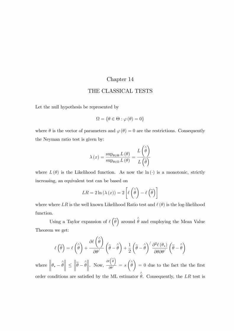
Chapter 14
THE CLASSICAL TESTS
Let the null hypothesis be represented by
Ω = θ ∈ Θ : ϕ (θ) = 0
where θ is the vector of parameters and ϕ (θ) = 0 are the restrictions. Consequently
the Neyman ratio test is given by:
λ (x) =supθ∈Θ L (θ)
supθ∈Ω L (θ)=
L
µ∧θ
¶L³eθ´
where L (θ) is the Likelihood function. As now the ln (·) is a monotonic, strictly
increasing, an equivalent test can be based on
LR = 2 ln (λ (x)) = 2
∙ µ∧θ
¶−
³eθ´¸where where LR is the well known Likelihood Ratio test and (θ) is the log-likelihood
function.
Using a Taylor expansion of³eθ´ around ∧
θ and employing the Mean Value
Theorem we get:
³eθ´ = µ∧θ
¶+
∂
µ∧θ
¶∂θ/
µeθ − ∧θ
¶+1
2
µeθ − ∧θ
¶/∂2 (θ∗)
∂θ∂θ/
µeθ − ∧θ
where
°°°°θ∗ − ∧θ
°°°° ≤ °°°°eθ − ∧θ
°°°°. Now, ∂
µ∧θ
¶∂θ/
= s
µ∧θ
¶= 0 due to the fact the the first
order conditions are satisfied by the ML estimator∧θ. Consequently, the LR test is

126 The Classical Tests
given by:
LR = 2
∙ µ∧θ
¶−
³eθ´¸ = −µeθ − ∧θ
¶/∂2 (θ∗)
∂θ∂θ/
µeθ − ∧θ
¶.
Now we know that
√n³eθ − θ0
´=
½Ik −
h_J (θ0)
i−1F / (θ0) [P (θ0)]
−1 F (θ0)
¾h_J (θ0)
i−1 s (θ0)√n+ op (1)
and√n
µ∧θ − θ0
¶=h_J (θ0)
i−1 s (θ0)√n+ op (1) .
Hence
√n
µeθ − ∧θ
¶= −
h_J (θ0)
i−1F / (θ0) [P (θ0)]
−1 F (θ0)h_J (θ0)
i−1 s (θ0)√n+ op (1)
and consequently
LR =
µh_J (θ0)
i−1F / (θ0) [P (θ0)]
−1 F (θ0)h_J (θ0)
i−1 s (θ0)√n
¶/µ−1n
∂2 (θ∗)
∂θ∂θ/
¶h_J (θ0)
i−1F / (θ0) [P (θ0)]
−1 F (θ0)h_J (θ0)
i−1 s (θ0)√n+ op (1) .
Now from assumption A5. we have
n−1H (θ) = −_
J (θ) + op (1) ,
θ∗ = θ0 + op (1) and P (θ0) = F (θ0)h_J (θ0)
i−1F / (θ0) .
Hence
LR =
µs (θ0)√
n
¶/ h_J (θ0)
i−1F / (θ0) [P (θ0)]
−1 F (θ0)h_J (θ0)
i−1 s (θ0)√n+ op (1) .
We can now state the following Theorem:
Theorem 52 Under the usual assumptions and under the null Hypothesis we have
that
LR = 2
∙ µ∧θ
¶−
³eθ´¸ d→ χ2r.

The Classical Tests 127
Proof: The Likelihood Ratio is written as
LR = (ξ0)/ Z0
hZ/0Z0
i−1Z/0ξ0 + op (1)
where h_J (θ0)
i−1/2 s (θ0)√n= ξ0, and Z0 =
h_J (θ0)
i−1/2F / (θ0) .
Now h_J (θ0)
i−1/2 s (θ0)√n
d→ N (0, Ik)
and Z0hZ/0Z0
i−1Z/0 is symmetric idempotent. Hence
r
µZ0hZ/0Z0
i−1Z/0
¶= tr
µZ0hZ/0Z0
i−1Z/0
¶= tr
µhZ/0Z0
i−1Z/0Z0
¶= tr (Ir) = r.
Consequently, we get the result. ¥TheWald test is based on the idea that if the restrictions are correct the vector
ϕ
µ∧θ
¶should be close to zero.
Expanding ϕµ∧θ
¶around ϕ (θ0) we get:
ϕ
µ∧θ
¶= ϕ (θ0) +
∂ϕ (θ∗)
∂θ/
µ∧θ − θ0
¶= F (θ∗)
µ∧θ − θ0
¶as under the null ϕ (θ0) = 0. Hence
√nϕ
µ∧θ
¶=√nF (θ∗)
µ∧θ − θ0
¶and consequently
√nϕ
µ∧θ
¶=√nF (θ0)
µ∧θ − θ0
¶+ op (1) .
Furthermore recall that
√n
µ∧θ − θ0
¶d→ N
∙0,³_J (θ0)
´−1¸.
Hence,√nϕ
µ∧θ
¶d→ N
∙0, F (θ0)
³_J (θ0)
´−1F / (θ0)
¸.

128 The Classical Tests
Let us now consider the following quadratic:
n
∙ϕ
µ∧θ
¶¸/ ∙F (θ0)
³_J (θ0)
´−1F / (θ0)
¸−1ϕ
µ∧θ
¶,
which is the square of the Mahalanobis distance of the√nϕ
µ∧θ
¶vector. However the
above quantity can not be considered as a statistic as it is a function of the unknown
parameter θ0. The Wald test is given by the above quantity if the unknown vector of
parameters θ0 is substituted by the ML estimator∧θ, i.e.
W =
∙ϕ
µ∧θ
¶¸/ "F
µ∧θ
¶µn_
J
µ∧θ
¶¶−1F /
µ∧θ
¶#−1ϕ
µ∧θ
=
∙ϕ
µ∧θ
¶¸/ "F
µ∧θ
¶µJ
µ∧θ
¶¶−1F /
µ∧θ
¶#−1ϕ
µ∧θ
¶,
where Jµ∧θ
¶is the estimated information matrix. In case that J
µ∧θ
¶does not have
an explicit formula it can be substituted by a consistent estimator, e.g. by
∧J = −
nXi=1
∂2µ∧θ
¶∂θ∂θ/
or by the asymptotically equivalent
∧J =
nXi=1
∂
µ∧θ
¶∂θ
∂
µ∧θ
¶∂θ/
.
Hence the Wald statistic is given by
W =
∙ϕ
µ∧θ
¶¸/ "F
µ∧θ
¶µ∧J
¶−1F /
µ∧θ
¶#−1ϕ
µ∧θ
¶.
Now we can prove the following Theorem:
Theorem 53 Under the usual regularity assumptions and the null hypothesis we that
W =
∙ϕ
µ∧θ
¶¸/ "F
µ∧θ
¶µ∧J
¶−1F /
µ∧θ
¶#−1ϕ
µ∧θ
¶d→ χ2r.
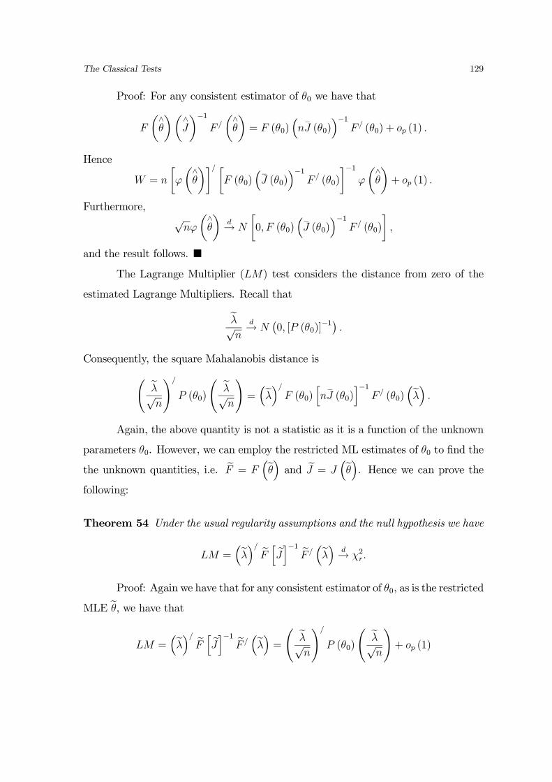
The Classical Tests 129
Proof: For any consistent estimator of θ0 we have that
F
µ∧θ
¶µ∧J
¶−1F /
µ∧θ
¶= F (θ0)
³n_
J (θ0)´−1
F / (θ0) + op (1) .
Hence
W = n
∙ϕ
µ∧θ
¶¸/ ∙F (θ0)
³_J (θ0)
´−1F / (θ0)
¸−1ϕ
µ∧θ
¶+ op (1) .
Furthermore,√nϕ
µ∧θ
¶d→ N
∙0, F (θ0)
³_J (θ0)
´−1F / (θ0)
¸,
and the result follows. ¥The Lagrange Multiplier (LM) test considers the distance from zero of the
estimated Lagrange Multipliers. Recall that
eλ√n
d→ N¡0, [P (θ0)]
−1¢ .Consequently, the square Mahalanobis distance isà eλ√
n
!/
P (θ0)
à eλ√n
!=³eλ´/ F (θ0) hn_J (θ0)i−1 F / (θ0)
³eλ´ .Again, the above quantity is not a statistic as it is a function of the unknown
parameters θ0. However, we can employ the restricted ML estimates of θ0 to find the
the unknown quantities, i.e. eF = F³eθ´ and eJ = J
³eθ´. Hence we can prove thefollowing:
Theorem 54 Under the usual regularity assumptions and the null hypothesis we have
LM =³eλ´/ eF h eJi−1 eF /
³eλ´ d→ χ2r.
Proof: Again we have that for any consistent estimator of θ0, as is the restricted
MLE eθ, we have thatLM =
³eλ´/ eF h eJi−1 eF /³eλ´ = Ã eλ√
n
!/
P (θ0)
à eλ√n
!+ op (1)

130 The Classical Tests
and by the asymptotic distribution of the Lagrange Multipliers we get the result. ¥
Now we have that the Restricted MLE satisfy the first order conditions of the
Lagrangian, i.e.
s³eθ´+ F /
³eθ´eλ = 0.Consequently the LM test can be expressed as:
LM =³s³eθ´´/ h eJi−1 s³eθ´ .
Now Rao has suggested to find the score vector and the information matrix of the
unrestricted model and evaluate them at the restricted MLE. Under this form the
LM statistic is called efficient score statistic as it measures the distance of the
score vector, evaluated at the restricted MLE, from zero.
14.1 The Linear Regression
Let us consider the classical linear regression model:
y = Xβ + u, u|X v N¡0, σ2In
¢where y is the n× 1 vector of endogenous variables, X is the n× k matrix of weakly
exogenous explanatory variables, β is the k × 1 vector of mean parameters and u is
the n× 1 vector of errors. Let us call the vector of parameters θ, i.e. θ/ =³β/, σ2
´a (k + 1)× 1 vector. The log-likelihood function is:
(θ) = −n2ln (2π)− n
2ln¡σ2¢− 12
(y −Xβ)/ (y −Xβ)
σ2.
The first order conditions are:
∂ (θ)
∂β=
X/ (y −Xβ)
σ2= 0
and∂ (θ)
∂σ2= − n
2σ2+1
2
(y −Xβ)/ (y −Xβ)
σ4= 0.

The Linear Regression 131
Solving the equations we get:
∧β =
¡X/X
¢−1X/y
∧σ2 =
∧u/∧u
n,
∧u = y −X
∧β.
Notice that the MLE of β is the same as OLS estimator. Something which is not true
for the MLE of σ2.
The Hessian is
H (θ) =∂2 (θ)
∂θ∂θ/=
⎛⎝ ∂2 (θ)
∂β∂β/∂2 (θ)∂β∂σ2
∂2 (θ)
∂σ2∂β/∂2 (θ)
∂(σ2)2
⎞⎠ =
⎛⎝ − 1σ2X/X − 1
2σ4X/u
− 12σ4
u/X n2σ4− u/u
σ6
⎞⎠ .
Hence the Information matrix is
J (θ) = E [−H (θ)] =
⎛⎝ 1σ2X/X 0
0 n2σ4
⎞⎠ ,
and the Cramer-Rao limit
J−1 (θ) =
⎛⎝ σ2¡X/X
¢−10
0 2σ4
n
⎞⎠ .
Notice that under normality, of the errors, the OLS estimator is asymptotically effi-
cient.
Let us now consider r linear constrains on the parameter vector β, i.e.
ϕ (β) = Qβ − q = 0 (14.1)
where Q is the r × k matrix of the restrictions (with r < k) and q a known vector.
Let us now form the Lagrangian, i.e.
L = (θ) + λ/ϕ (β) = (θ) + ϕ/ (β)λ = (θ) + (Qβ − q)/ λ,
where λ is the vector of the r Lagrange Multipliers. The first order conditions are:
∂L
∂β=
∂ (θ)
∂β+Q/λ =
X/ (y −Xβ)
σ2+Q/λ = 0 (14.2)

132 The Classical Tests
∂L
∂σ2=
∂ (θ)
∂σ2= − n
2σ2+1
2
(y −Xβ)/ (y −Xβ)
σ4= 0 (14.3)
and∂L
∂λ= Qβ − q = 0. (14.4)
Now from (14.2) we have that
X/y = X/Xβ − σ2Q/λ (14.5)
and it follows that
Q¡X/X
¢−1X/y = Q
¡X/X
¢−1X/Xβ − σ2Q
¡X/X
¢−1Q/λ.
Hence
Q¡X/X
¢−1X/y = Qβ − σ2Q
¡X/X
¢−1Q/λ.
It follows that
Qβ −QVQ/λ = Q∧β,
where∧β =
¡X/X
¢−1X/y and V = σ2
¡X/X
¢−1.
Now from (14.4) we have that Qβ = q. Hence we get
λ = −£QVQ/
¤−1µQ∧β − q
¶. (14.6)
Substituting out λ from (14.5) employing the above and solving for β we get:
eβ = ∧β −
¡X/X
¢−1Q/hQ¡X/X
¢−1Q/i−1µ
Q∧β − q
¶.
Solving (14.3) we get that
eσ2 = (eu)/ eun
, eu = y −Xeβ,and from (14.6) we get:
eλ = − hQeV Q/i−1µ
Q∧β − q
¶, eV = eσ2 ¡X/X
¢−1.

The Linear Regression 133
The above 3 formulae give the restricted MLEs.
Now the Wald test for the linear restrictions in (14.1) is given by
W =
µQ∧β − q
¶/ ∙Q∧V Q/
¸−1µQ∧β − q
¶.
The restricted and unrestricted residuals are given by
eu = y −Xeβ, and∧u = y −X
∧β.
Hence eu = ∧u+X
µ∧β − eβ
and consequently, if X/∧u = 0, i.e. the regression has a constant we have that
eu/eu = ∧u/∧u+
µ∧β − eβ¶/
X/X
µ∧β − eβ¶ .
It follows that
eu/eu− ∧u/∧u =
µQ∧β − q
¶/ hQ¡X/X
¢−1Q/i−1µ
Q∧β − q
¶.
Hence the Wald test is given by
W = neu/eu− ∧
u/∧u
∧u/∧u
.
The LR test is given by
LR = 2
∙ µ∧θ
¶−
³eθ´¸ = n ln
Ãeu/eu∧u/∧u
!
and the LM test is
LM = neu/eu− ∧
u/∧ueu/eu
as
LM =³eλ´/ eF h eJi−1 eF /
³eλ´ = µQ∧β − q
¶/ hQeV Q/
i−1µQ∧β − q
¶.
We can now state a well known result.

134 The Classical Tests
Theorem 55 Under the classical assumptions of the Linear Regression Model we
have that
W ≥ LR ≥ LM.
Proof: The three test can be written as
W = n (r − 1) , LR = n ln (r) , LM = n
µ1− 1
r
¶,
where r = eu/eu∧u/∧u≥ 1. Now we know that ln (x) ≥ x−1
xand the result follows by
considering x = r and x = 1/r.
14.2 Autocorrelation
Apply the LM test to test the hypothesis that ρ = 0 in the following model
yt = x/tβ + ut, ut = ρut−1 + εt, εt
i.i.d.v N¡0, σ2
¢.
Discuss the advantages of this LM test over the Wald and LR tests of this hypothesis.
First notice that from ut = ρut−1 + εt we get that
E (ut) = ρE (ut−1) +E (εt) = ρE (ut−1)
as E (εt) = 0 and for |ρ| < 1 we get that
E (ut)− ρE (ut−1) = 0⇒ E (ut) = 0
as E (ut) = E (ut−1) independent of t. Furthermore
V ar (ut) = E¡u2t¢= ρ2E
¡u2t−1
¢+E
¡ε2t¢+ 2ρE (ut−1εt) = ρ2E
¡u2t−1
¢+ σ2
as the first equality follows from the fact that E (ut) = 0, and the last from the fact
that
E (ut−1εt) = E [ut−1E (εt|It−1)] = E [ut−10] = 0

Autocorrelation 135
where It−1 the information set at time t − 1, i.e. the sigma-field generated by
εt−1, εt−2, .... Hence
E¡u2t¢− ρ2E
¡u2t−1
¢= σ2 ⇒ E
¡u2t¢=
σ2
1− ρ2
as E (u2t ) = E¡u2t−1
¢independent of t.
Substituting out ut we get
yt = x/tβ + ρut−1 + εt,
and observing that ut−1 = yt−1 − x/t−1β we get
yt = x/tβ + ρ
³yt−1 − x
/t−1β
´+ εt ⇒ εt = yt − x
/tβ − ρyt−1 + x
/t−1βρ
where by assumption the ε0ts are i.i.d. Hence the log-likelihood function is
l (θ) = −T2ln (2π)− T
2ln¡σ2¢−
TXt=1
³yt − x
/tβ − ρyt−1 + x
/t−1βρ
´22σ2
,
where we assume that y−1 = 0, and x−1 = 0. as we do not have any observations
for t = −1. In any case, given that |ρ| < 1, the first observation will not affect the
distribution LM test, as it is based in asymptotic theory, i.e. T →∞. The first order
conditions are:
∂l
∂β=
TXt=1
³yt − x
/tβ − ρyt−1 + x
/t−1βρ
´(xt − xt−1ρ)
σ2
∂l
∂ρ=
TXt=1
³yt − x
/tβ − ρyt−1 + x
/t−1βρ
´³yt−1 − x
/t−1β
´σ2
=TXt=1
εtut−1σ2
,
∂l
∂σ2= − T
2σ2+
TXt=1
³yt − x
/tβ − ρyt−1 + x
/t−1βρ
´22σ4
= − T
2σ2+
TXt=1
ε2t2σ4
.
The second derivatives are:
∂2l
∂β∂β/= −
TXt=1
(xt − xt−1ρ)³x/t − x
/t−1ρ
´σ2

136 The Classical Tests
∂2l
∂ρ2= −
TXt=1
³yt−1 − x
/t−1β
´2σ2
= −TXt=1
u2t−1σ2
,
∂2l
∂ (σ2)2=
T
2σ4−
TXt=1
³yt − x
/tβ − ρyt−1 + x
/t−1βρ
´2σ6
=T
2σ4−
TXt=1
ε2tσ6
.
∂2l
∂β∂ρ= −
TXt=1
³yt−1 − x
/t−1β
´³x/t − x
/t−1ρ
´+³yt − x
/tβ − ρyt−1 + x
/t−1βρ
´³x/t−1
´σ2
=
= −TXt=1
ut−1³x/t − x
/t−1ρ
´+ εt
³x/t−1
´σ2
∂2l
∂ρ∂σ2= −
TXt=1
³yt − x
/tβ − ρyt−1 + x
/t−1βρ
´³yt−1 − x
/t−1β
´σ4
= −TXt=1
εtut−1σ4
,
∂2l
∂β∂σ2= −
TXt=1
³yt − x
/tβ − ρyt−1 + x
/t−1βρ
´³x/t − x
/t−1ρ
´σ4
= −TXt=1
εt³x/t − x
/t−1ρ
´σ4
Notice now that the Information Matrix J is
J (θ) = −E [H (θ)] =
⎡⎢⎢⎢⎣PT
t=1
(xt−xt−1ρ)³x/t−x
/t−1ρ
´σ2
0 0
0 T1−ρ2 0
0 0 T2σ4
⎤⎥⎥⎥⎦asE
∙ut−1
³x/t−x
/t−1ρ
´+εt
³x/t−1
´σ2
¸= 0, E
∙εt³x/t−x
/t−1ρ
´σ4
¸= 0, E
hPTt=1
εtut−1σ4
i= 0, E
hε2tσ6
i=
1σ4, E
hu2t−1σ2
i=
E(u2t−1)σ2
= 11−ρ2 , i.e. the matrix is block diagonal between β, ρ, and σ
2.
Consequently the LM test has the form
LM = s/ρJ−1ρρ sρ =
(sρ)2
Jρρ
as sρ =PT
t=1εtut−1σ2
, Jρρ = T1−ρ2 . All these quantities evaluated under the null.
Hence under H0 : ρ = 0 we have that
Jρρ = T, and ut = εt

Autocorrelation 137
i.e. there is no autocorrelation. Consequently, we can estimate β by simple OLS, as
OLS and ML result in the same estimators and σ2 by the ML estimator, i.e.
eβ = Ã TXt=1
xtx/t
!−1 TXt=1
xtyt, and eσ2 = eu/euT=
PTt=1 eu2tT
,
where eut = yt − x/teβ = eεt the OLS residuals. Hence
LM =
³PTt=1
euteut−1fσ2´2
T= T
ÃTXt=1
euteut−1!2Ã TXt=1
eu2t!−2
.

138 The Classical Tests
Book References1. T. Amemiya: Advanced Econometrics.
2. E. Berndt: The Practice of Econometrics: Classic and Cotemporary
3. G. Box and G. Jenkins (1976) TimeSeries Analysis forecasting and Control.
K. Cuthbertson, S.G. Hall and M. P. Taylor: Applied Econometric Techniques.
4. R. Davidson and J. MacKinnon: Econometric Theory and Methods.
5. C. Gourieroux and A. Monfort: Statistics and Econometric Models, Vol I
and II.
6. W.H. Greene: Econometric Analysis.
7. J. Hamilton Time Series Analysis
8. A. Harvey: The Econometric Analysis of Time Series.
9. A. Harvey: Time Series Models.
10. J. Johnston: Econometric Methods.
11. G. Judge, R. Hill, H. Lutkepohl and T. Lee: Introduction to the Theory
and Practice of Econometrics.
12. R. Pindyck and D. Rubinfeld: Econometric Models and Economic Fore-
casts.
13. P. Ruud: An Introduction to Classical Econometric Theory.
14. R. Serfling: Approximation Theorems of Mathematical Statistics.
15. H White: Asymptotic Theory for Econometricians.


![Introduction to Probability Theory and Statistics [Matzinger]](https://img.dokumen.tips/doc/110x75/55cf866c550346484b977309/introduction-to-probability-theory-and-statistics-matzinger.jpg)


