Introduction to Probability Theory and Statisticsmplab.ucsd.edu/tutorials/ProbabilityAndStats.pdf · Introduction to Probability Theory and Statistics Cop yright @ Javier R. Mo vellan,

Introduction to Probability Theory andStatistics

Copyright @ Javier R. Movellan, 2004-2008

August 21, 2008

2

Contents

1 Probability 71.1 Intuitive Set Theory . . . . . . . . . . . . . . . . . . . . . . . . . 101.2 Events . . . . . . . . . . . . . . . . . . . . . . . . . . . . . . . . 141.3 Probability measures . . . . . . . . . . . . . . . . . . . . . . . . 141.4 Joint Probabilities . . . . . . . . . . . . . . . . . . . . . . . . . 161.5 Conditional Probabilities . . . . . . . . . . . . . . . . . . . . . 161.6 Independence of 2 Events . . . . . . . . . . . . . . . . . . . . . 171.7 Independence of n Events . . . . . . . . . . . . . . . . . . . . . 171.8 The Chain Rule of Probability . . . . . . . . . . . . . . . . . . 191.9 The Law of Total Probability . . . . . . . . . . . . . . . . . . . 201.10 Bayes’ Theorem . . . . . . . . . . . . . . . . . . . . . . . . . . 211.11 Exercises . . . . . . . . . . . . . . . . . . . . . . . . . . . . . . 22

2 Random variables 252.1 Probability mass functions. . . . . . . . . . . . . . . . . . . . . . 282.2 Probability density functions. . . . . . . . . . . . . . . . . . . . . 302.3 Cumulative Distribution Function. . . . . . . . . . . . . . . . . . 322.4 Exercises . . . . . . . . . . . . . . . . . . . . . . . . . . . . . . 34

3 Random Vectors 373.1 Joint probability mass functions . . . . . . . . . . . . . . . . . . 373.2 Joint probability density functions . . . . . . . . . . . . . . . . . 373.3 Joint Cumulative Distribution Functions . . . . . . . . . . . . . . 383.4 Marginalizing . . . . . . . . . . . . . . . . . . . . . . . . . . . . 383.5 Independence . . . . . . . . . . . . . . . . . . . . . . . . . . . . 393.6 Bayes’ Rule for continuous data and discrete hypotheses . . . . . 40

3.6.1 A useful version of the LTP . . . . . . . . . . . . . . . . 413.7 Random Vectors and Stochastic Processes . . . . . . . . . . . . . 42

3

4 CONTENTS

4 Expected Values 434.1 Fundamental Theorem of Expected Values . . . . . . . . . . . . . 444.2 Properties of Expected Values . . . . . . . . . . . . . . . . . . . 464.3 Variance . . . . . . . . . . . . . . . . . . . . . . . . . . . . . . . 47

4.3.1 Properties of the Variance . . . . . . . . . . . . . . . . . 484.4 Appendix: Using Standard Gaussian Tables . . . . . . . . . . . . 514.5 Exercises . . . . . . . . . . . . . . . . . . . . . . . . . . . . . . 52

5 The precision of the arithmetic mean 535.1 The sampling distribution of the mean . . . . . . . . . . . . . . . 54

5.1.1 Central Limit Theorem . . . . . . . . . . . . . . . . . . . 555.2 Exercises . . . . . . . . . . . . . . . . . . . . . . . . . . . . . . 56

6 Introduction to Statistical Hypothesis Testing 596.1 The Classic Approach . . . . . . . . . . . . . . . . . . . . . . . . 596.2 Type I and Type II errors . . . . . . . . . . . . . . . . . . . . . . 61

6.2.1 Specifications of a decision system . . . . . . . . . . . . . 636.3 The Bayesian approach . . . . . . . . . . . . . . . . . . . . . . . 636.4 Exercises . . . . . . . . . . . . . . . . . . . . . . . . . . . . . . 65

7 Introduction to Classic Statistical Tests 677.1 The Z test . . . . . . . . . . . . . . . . . . . . . . . . . . . . . . 67

7.1.1 Two tailed Z test . . . . . . . . . . . . . . . . . . . . . . 677.1.2 One tailed Z test . . . . . . . . . . . . . . . . . . . . . . 69

7.2 Reporting the results of a classical statistical test . . . . . . . . . . 717.2.1 Interpreting the results of a classical statistical test . . . . 71

7.3 The T-test . . . . . . . . . . . . . . . . . . . . . . . . . . . . . . 727.3.1 The distribution of T . . . . . . . . . . . . . . . . . . . . 737.3.2 Two-tailed T-test . . . . . . . . . . . . . . . . . . . . . . 747.3.3 A note about LinuStats . . . . . . . . . . . . . . . . . . . 76

7.4 Exercises . . . . . . . . . . . . . . . . . . . . . . . . . . . . . . 767.5 Appendix: The sample variance is an umbiased estimate of the

population variance . . . . . . . . . . . . . . . . . . . . . . . . . 78

8 Intro to Experimental Design 818.1 An example experiment . . . . . . . . . . . . . . . . . . . . . . . 818.2 Independent, Dependent and Intervening Variables . . . . . . . . 838.3 Control Methods . . . . . . . . . . . . . . . . . . . . . . . . . . 84

CONTENTS 5

8.4 Useful Concepts . . . . . . . . . . . . . . . . . . . . . . . . . . . 878.5 Exercises . . . . . . . . . . . . . . . . . . . . . . . . . . . . . . 89

9 Experiments with 2 groups 939.1 Between Subjects Experiments . . . . . . . . . . . . . . . . . . . 93

9.1.1 Within Subjects Experiments . . . . . . . . . . . . . . . . 969.2 Exercises . . . . . . . . . . . . . . . . . . . . . . . . . . . . . . 98

10 Factorial Experiments 9910.1 Experiments with more than 2 groups . . . . . . . . . . . . . . . 9910.2 Interaction Effects . . . . . . . . . . . . . . . . . . . . . . . . . . 101

11 Confidence Intervals 103

A Useful Mathematical Facts 107

B Set Theory 115B.1 Proofs and Logical Truth . . . . . . . . . . . . . . . . . . . . . . 118B.2 The Axioms of Set Theory . . . . . . . . . . . . . . . . . . . . . 119

B.2.1 Axiom of Existence: . . . . . . . . . . . . . . . . . . . . 119B.2.2 Axiom of Equality: . . . . . . . . . . . . . . . . . . . . . 120B.2.3 Axiom of Pair: . . . . . . . . . . . . . . . . . . . . . . . 120B.2.4 Axiom of Separation: . . . . . . . . . . . . . . . . . . . . 121B.2.5 Axiom of Union: . . . . . . . . . . . . . . . . . . . . . . 122B.2.6 Axiom of Power: . . . . . . . . . . . . . . . . . . . . . . 123B.2.7 Axiom of Infinity: . . . . . . . . . . . . . . . . . . . . . 124B.2.8 Axiom of Image: . . . . . . . . . . . . . . . . . . . . . . 124B.2.9 Axiom of Foundation: . . . . . . . . . . . . . . . . . . . 125B.2.10 Axiom of Choice: . . . . . . . . . . . . . . . . . . . . . . 125

6 CONTENTS

Chapter 1

Probability

Probability theory provides a mathematical foundation to concepts such as “proba-bility”, “information”, “belief”, “uncertainty”, “confidence”, “randomness”, “vari-ability”, “chance” and “risk”. Probability theory is important to empirical sci-entists because it gives them a rational framework to make inferences and testhypotheses based on uncertain empirical data. Probability theory is also usefulto engineers building systems that have to operate intelligently in an uncertainworld. For example, some of the most successful approaches in machine per-ception (e.g., automatic speech recognition, computer vision) and artificial intel-ligence are based on probabilistic models. Moreover probability theory is alsoproving very valuable as a theoretical framework for scientists trying to under-stand how the brain works. Many computational neuroscientists think of the brainas a probabilistic computer built with unreliable components, i.e., neurons, anduse probability theory as a guiding framework to understand the principles ofcomputation used by the brain. Consider the following examples:

• You need to decide whether a coin is loaded (i.e., whether it tends to favorone side over the other when tossed). You toss the coin 6 times and in allcases you get “Tails”. Would you say that the coin is loaded?

• You are trying to figure out whether newborn babies can distinguish greenfrom red. To do so you present two colored cards (one green, one red)to 6 newborn babies. You make sure that the 2 cards have equal overallluminance so that they are indistinguishable if recorded by a black and whitecamera. The 6 babies are randomly divided into two groups. The first groupgets the red card on the left visual field, and the second group on the right

7

8 CHAPTER 1. PROBABILITY

visual field. You find that all 6 babies look longer to the red card than thegreen card. Would you say that babies can distinguish red from green?

• A pregnancy test has a 99 % validity (i.e., 99 of of 100 pregnant women testpositive) and 95 % specificity (i.e., 95 out of 100 non pregnant women testnegative). A woman believes she has a 10 % chance of being pregnant. Shetakes the test and tests positive. How should she combine her prior beliefswith the results of the test?

• You need to design a system that detects a sinusoidal tone of 1000Hz in thepresence of white noise. How should design the system to solve this taskoptimally?

• How should the photo receptors in the human retina be interconnected tomaximize information transmission to the brain?

While these tasks appear different from each other, they all share a common prob-lem: The need to combine different sources of uncertain information to make ra-tional decisions. Probability theory provides a very powerful mathematical frame-work to do so. Before we go into mathematical aspects of probability theory Ishall tell you that there are deep philosophical issues behind the very notion ofprobability. In practice there are three major interpretations of probability, com-monly called the frequentist, the Bayesian or subjectivist, and the axiomatic ormathematical interpretation.

1. Probability as a relative frequencyThis approach interprets the probability of an event as the proportion oftimes such ane event is expected to happen in the long run. Formally, theprobability of an event E would be the limit of the relative frequency ofoccurrence of that event as the number of observations grows large

P (E) = limn!"

nE

n(1.1)

where nE is the number of times the event is observed out of a total ofn independent experiments. For example, we say that the probability of“heads” when tossing a coin is 0.5. By that we mean that if we toss a coinmany many times and compute the relative frequency of “heads” we expectfor that relative frequency to approach 0.5 as we increase the number oftosses.

9

This notion of probability is appealing because it seems objective and tiesour work to the observation of physical events. One difficulty with the ap-proach is that in practice we can never perform an experiment an infinitenumber of times. Note also that this approach is behaviorist, in the sensethat it defines probability in terms of the observable behavior of physicalsystems. The approach fails to capture the idea of probability as internalknowledge of cognitive systems.

2. Probability as uncertain knowledge.

This notion of probability is at work when we say things like “I will proba-bly get an A in this class”. By this we mean something like “Based on whatI know about myself and about this class, I would not be very surprised if Iget an A. However, I would not bet my life on it, since there are a multitudeof factors which are difficult to predict and that could make it impossiblefor me to get an A”. This notion of probability is “cognitive” and does notneed to be directly grounded on empirical frequencies. For example, I cansay things like “I will probably die poor” even though I will not be able torepeat my life many times and count the number of lives in which I die poor.

This notion of probability is very useful in the field of machine intelligence.In order for machines to operate in natural environments they need knowl-edge systems capable of handling the uncertainty of the world. Probabilitytheory provides an ideal way to do so. Probabilists that are willing to rep-resent internal knowledge using probability theory are called “Bayesian”,since Bayes is recognized as the first mathematician to do so.

3. Probability as a mathematical model. Modern mathematicians avoid thefrequentist vs. Bayesian controversy by treating probability as a mathemat-ical object. The role of mathematics here is to make sure probability theoryis rigorously defined and traceable to first principles. From this point ofview it is up to the users of probability theory to apply it to whatever theysee fit. Some may want to apply it to describe limits of relative frequencies.Some may want to apply it to describe subjective notions of uncertainty, orto build better computers. This is not necessarily of concern to the math-ematician. The application of probability theory to those domains will beultimately judged by its usefulness.


1.1 Intuitive Set TheoryWe need a few notions from set theory before we jump into probability theory.In doing so we will use intuitive or “naive” definitions. This intuitive approachprovides good mnemonics and is sufficient for our purposes but soon runs intoproblems for more advanced applications. For a more rigorous definition of settheoretical concepts and an explanation of the limitations of the intuitive approachyou may want to take a look at the Appendix.

• Set: A set is a collection of elements. Sets are commonly represented usingcurly brackets containing a collection of elements separated by commas.For example

A = {1, 2, 3} (1.2)

tells us that A is a set whose elements are the first 3 natural numbers. Setscan also be represented using a rule that identifies the elements of the set.The prototypical notation is as follows

{x : x follows a rule} (1.3)

For example,

{x : x is a natural number and x is smaller than 4 } (1.4)

• Outcome Space: The outcome space is a set whose elements are all thepossible basic outcomes of an experiment.1 The sample space is also calledsample space, reference set, and universal set and it is commonly repre-sented with the capital Greek letter “omega”, !. We call the elements of thesample space “outcomes” and represent them symbolically with the smallGreek letter “omega”, !.

Example 1: If we roll a die, the outcome space could be

! = {1, 2, 3, 4, 5, 6} (1.5)

In this case the symbol ! could be used to represent either 1,2,3,4,5 or 6.1The empty set is not a valid sample space.

1.1. INTUITIVE SET THEORY 11

Example 2: If we toss a coin twice, we can observe 1 of 4 outcomes:(Heads, Heads), (Heads, Tails), (Tails, Heads), (Tails, Tails). In this case wecould use the following outcome space

! = {(H, H), (H, T ), (T, H), (T, T )} (1.6)

and the symbol ! could be used to represent either (H, H), or (H, T ), or(T, H), or (T, T ). Note how in this case each basic outcome contains 2elements. If we toss a coin n times each basic outcome ! would contain nelements.

• Singletons: A singleton is a set with a single element. For example the set{4} is a singleton, since it only has one element. On the other hand 4 is nota singleton since it is an element not a set.2

• Element inclusion: We use the symbol ! to represent element inclusion.The expression ! ! A tells us that ! is an element of the set A. Theexpression ! "! A tells us that ! is not an element of the set A. For example,1 ! {1, 2} is true since 1 is an element of the set {1, 2}. The expression{1} ! {{1}, 2} is also true since the singleton {1} is an element of the set{{1}, 2}. The expression {1} "! {1, 2} is also true, since the set {1} is notan element of the set {1, 2}.

• Set inclusion: We say that the set A is included in the set B or is a subset ofB if all the elements of A are also elements of B. We represent set inclusionwith the symbol #. The expression A # B tells us that both A and B aresets and that all the elements of A are also elements of B. For example theexpression {1} # {1, 2} is true since all the elements of the set {1} are inthe set {1, 2}. On the other hand 1 # {1, 2} is not true since 1 is an element,not a set.3

• Set equality: Two sets A and B are equal if all elements of A belong to Band all elements of B belong to A. In other words, if A # B and B # A.For example the sets {1, 2, 3} and {3, 1, 1, 2, 1} are equal.

• Set Operations: There are 3 basic set operations:2The distinction between elements and sets does not exist in axiomatic set theory, but it is

useful when explaining set theory in an intuitive manner.3For a more rigorous explanation see the Appendix on axiomatic set theory.


1. Union: The union of two sets A and B is another set that includes allelements of A and all elements of B. We represent the union operatorwith this symbol $For example, if A = {1, 3, 5} and B = {2, 3, 4}, then A $ B ={1, 2, 3, 4, 5}. More generally

A $ B = {! : ! ! A or ! ! B} (1.7)

In other words, the set A $ B is the set of elements with the propertythat they either belong to the set A or to the set B.

2. Intersection: The intersection of two sets A and B is another set Csuch that all elements in C belong to A and to B. The intersectionoperator is symbolized as %. If A = {1, 3, 5} and B = {2, 3, 4} thenA % B = {3}. More generally

A % B = {! : ! ! A and ! ! B} (1.8)

3. Complementation: The complement of a set A with respect to a ref-erence set ! is the set of all elements of ! which do not belong to A.The complement of A is represented as Ac. For example, if the univer-sal set is {1, 2, 3, 4, 5, 6} then the complement of {1, 3, 5} is {2, 4, 6}.More generally

Ac = {! : ! ! ! and ! "! A} (1.9)

• Empty set: The empty set is a set with no elements. We represent the nullset with the symbol !. Note !c = !, !c = !, and for any set A

A $ ! = A (1.10)A % ! = ! (1.11)

• Disjoint sets: Two sets are disjoint if they have no elements in common,i.e., their intersection is the empty set. For example, the sets {1, 2} and {1}are not disjoint since they have an element in common.

• Collections: A collection of sets is a set of sets, i.e., a set whose elementsare sets. For example, if A and B are the sets defined above, the set {A, B}is a collection of sets.

1.1. INTUITIVE SET THEORY 13

• Power set: The power set of a set A is the a collection of all possible setsof A. We represent it as P(A). For example, if A = {1, 2, 3} then

P(A) = {!, {1}, {2}, {3}, {1, 2}, {1, 3}, {2, 3}, A} (1.12)

Note that 1 is not an element of P(A) but {1} is. This is because 1 is anelement of A, not a set of A.

• Collections closed under set operations: A collection of sets is closedunder set operations if any set operation on the sets in the collection resultsin another set which still is in the collection. If A = {1, 3, 5} and B ={2, 3, 4}, the collection C = {A, B} is not closed because the set A % B ={3} does not belong to the collection. The collection C = {!, !} is closedunder set operations, all set operations on elements of C produce another setthat belongs to C. The power set of a set is always a closed collection.

• Sigma algebra: A sigma algebra is a collection of sets which is closed whenset operations are applied to its members a countable number of times. Thepower set of a set is always a sigma algebra.

• Natural numbers: We use the symbol N to represent the natural numbers,i.e., {1, 2, 3, . . .}. One important property of the natural numbers is that ifx ! N then x + 1 ! N.

• Integers: We use the symbol Z to represent the set of integers, i.e., {. . . ,&3, &2, &1, 0, 1, 2, 3, . . .}. Note N # Z. One important property of thenatural numbers is that if x ! Z then x + 1 ! Z and x & 1 ! Z .

• Real numbers: We use the symbol R to represent the real numbers, i.e.,numbers that may have an infinite number of decimals. For example, 1,2.35, &4/123,

'2, and ", are real numbers. Note N # Z # R.

• Cardinality of sets:

– We say that a set is finite if it can be put in one-to-one correspondencewith a set of the form {1, 2, . . . , n}, where n is a fixed natural number.

– We say that a set is infinite countable if it can be put in one-to-onecorrespondence with the natural numbers.

– We say that a set is countable if it is either finite or infinite countable.


– We say that a set is infinite uncountable if it has a subset that can beput in one-to-one correspondence with the natural numbers, but the setitself cannot be put in such a correspondence. This includes sets thatcan be put in one-to-one correspondence with the real numbers.

1.2 EventsWe have defined outcomes as the elements of a reference set !. In practice weare interested in assigning probability values not only to outcomes but also tosets of outcomes. For example we may want to know the probability of gettingan even number when rolling a die. In other words, we want the probability ofthe set {2, 4, 6}. In probability theory set of outcomes to which we can assignprobabilities are called events. The collection of all events is called the eventspace and is commonly represented with the letter F . Not all collections of setsqualify as event spaces. To be an event space, the collection of sets has to be asigma algebra (i.e., it has to be closed under set operations). Here is an example:

Example: Consider the sample space ! = {1, 2, 3, 4, 5, 6}. Is the collection ofsets {{1, 2, 3}, {4, 5, 6}} a valid event space?Answer: No, it is not a valid event space because the union of {1, 2, 3} and{4, 5, 6} is the set ! = {1, 2, 3, 4, 5, 6} which does not belong to F . On the otherhand the set {!, {1, 2, 3}, {4, 5, 6}, !} is a valid event space. Any set operationusing the sets in F results into another set which is in F .

Note: The outcome space ! and the event space F are different sets. For ex-ample if the outcome space were ! = {H, T} a valid event space would beF = {!, !, {H}, {T}}. Note that ! "= F . The outcome space contains thebasic outcomes of an experiments. The event space contains sets of outcomes.

1.3 Probability measuresWhen we say that the probability of rolling an even number is 0.5, we can thinkof this as an assignment of a number (i.e., 0.5) to a set ,i.e., to the set {2, 4, 6}.Mathematicians think of probabilities as function that “measures” sets, thus thename probability measure. For example, if the probability of rolling an evennumber on a die is 0.5, we would say that the probability measure of the set

1.3. PROBABILITY MEASURES 15

{2, 4, 6} is 0.5. Probability measures are commonly represented with the letterP (capitalized). Probability measures have to follow three constraints, which areknown as Kolmogorov’s axioms:

1. The probability measure of events has to be larger or equal to zero: P (A) (0 for all A ! F .

2. The probability measure of the reference set is 1

P (!) = 1 (1.13)

3. If the sets A1, A2, . . . ! F are disjoint then

P (A1 $ A2 $ · · · ) = P (A1) + P (A2) + · · · (1.14)

Example 1: A fair coin. We can construct a probability space to describethe behavior of a coin. The outcome space consists of 2 elements, represent-ing heads and tails ! = {H, T}. Since ! is finite, we can use as the eventspace the set of all sets in !, also known as the power set of !. In our case,F = {{H}, {T}, {H, T}, !}. Note F is closed under set operations so we canuse it as an event space.

The probability measure P in this case is totally defined if we simply sayP ({H}) = 0.5. The outcome of P for all the other elements of F can be inferred:we already know P ({H}) = 0.5 and P ({H, T}) = 1.0. Note the sets {H} and{T} are disjoint, moreover {H} $ {T} = !, thus using the probability axioms

P ({H, T}) = 1 = P ({H}) + P ({T}) = 0.5 + P ({T}) (1.15)

from which it follows P ({T}) = 0.5. Finally we note that ! and ! are disjointand their union is !, using the probability axioms it follows that

1 = P (!) = P (! $ !) = P (!) + P (!) (1.16)

Thus P (!) = 0. Note P qualifies as a probability measure: for each element ofF it assigns a real number and the assignment is consistent with the three axiomof probability.

Example 2: A fair die. In this case the outcome space is ! = {1, 2, 3, 4, 5, 6},the event space is the power set of !, the set of all sets of !, F = P(!), andP ({i}) = 1/6, for i = 1, . . . , 6. I will refer to this as the fair die probabilityspace.


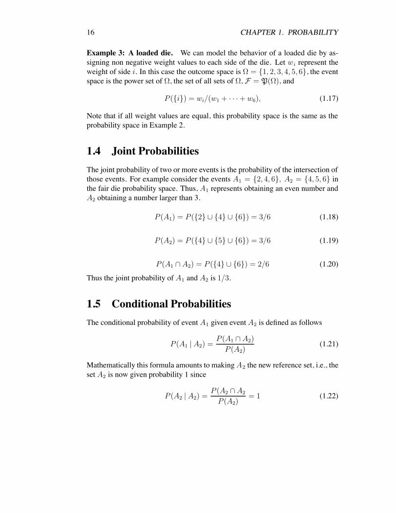
Example 3: A loaded die. We can model the behavior of a loaded die by as-signing non negative weight values to each side of the die. Let wi represent theweight of side i. In this case the outcome space is ! = {1, 2, 3, 4, 5, 6}, the eventspace is the power set of !, the set of all sets of !, F = P(!), and

P ({i}) = wi/(w1 + · · ·+ w6), (1.17)

Note that if all weight values are equal, this probability space is the same as theprobability space in Example 2.

1.4 Joint ProbabilitiesThe joint probability of two or more events is the probability of the intersection ofthose events. For example consider the events A1 = {2, 4, 6}, A2 = {4, 5, 6} inthe fair die probability space. Thus, A1 represents obtaining an even number andA2 obtaining a number larger than 3.

P (A1) = P ({2} $ {4} $ {6}) = 3/6 (1.18)

P (A2) = P ({4} $ {5} $ {6}) = 3/6 (1.19)

P (A1 % A2) = P ({4} $ {6}) = 2/6 (1.20)

Thus the joint probability of A1 and A2 is 1/3.

1.5 Conditional ProbabilitiesThe conditional probability of event A1 given event A2 is defined as follows

P (A1 | A2) =P (A1 % A2)

P (A2)(1.21)

Mathematically this formula amounts to making A2 the new reference set, i.e., theset A2 is now given probability 1 since

P (A2 | A2) =P (A2 % A2

P (A2)= 1 (1.22)

1.6. INDEPENDENCE OF 2 EVENTS 17

Intuitively, Conditional probability represents a revision of the original probabilitymeasure P . This revision takes into consideration the fact that we know the eventA2 has happened with probability 1. In the fair die example,

P (A1 | A2) =1/3

3/6=

2

3(1.23)

in other words, if we know that the toss produced a number larger than 3, theprobability that the number is even is 2/3.

1.6 Independence of 2 EventsThe notion of independence is crucial. Intuitively two events A1 and A2 are inde-pendent if knowing that A2 has happened does not change the probability of A1.In other words

P (A1 | A2) = P (A1) (1.24)More generally we say that the events A and A2 are independent if and only if

P (A1 % A2) = P (A1)P (A2) (1.25)

In the fair die example, P (A1 | A2) = 1/3 and P (A1) = 1/2, thus the two eventsare not independent.

1.7 Independence of n EventsWe say that the events A1, . . . , An are independent if and only if the followingconditions are met:

1. All pairs of events with different indexes are independent, i.e.,

P (Ai % Aj) = P (Ai)P (Aj) (1.26)

for all i, j ! {1, 2, . . . , n} such that i "= j.

2. For all triplets of events with different indexes

P (Ai % Aj % Ak) = P (Ai)P (Aj)P (Ak) (1.27)

for all i, j, k ! {1, . . . , n} such that i "= j "= k.


3. Same idea for combinations of 3 sets, 4 sets, . . .

4. For the n-tuple of events with different indexes

P (A1 % A2 % · · · % An) = P (A1)P (A2) · · ·P (An) (1.28)

You may want to verify that 2n & n & 1 conditions are needed to check whethern events are independent. For example, 23 & 3 & 1 = 4 conditions are needed toverify whether 3 events are independent.

Example 1: Consider the fair-die probability space and let A1 = A2 = {1, 2, 3},and A3 = {3, 4, 5, 6}. Note

P (A1 % A2 % A3) = P ({3}) = P (A1)P (A2)P (A3) = 1/6 (1.29)

HoweverP (A1 % A2) = 3/6 "= P (A1)P (A2) = 9/36 (1.30)

Thus A1, A2, A3 are not independent.

Example 2: Consider a probability space that models the behavior a weighteddie with 8 sides: ! = (1, 2, 3, 4, 5, 6, 7, 8), F = P(!) and the die is weighted sothat

P ({2}) = P ({3}) = P ({5}) = P ({8}) = 1/4 (1.31)P ({1}) = P ({4}) = P ({6}) = P ({7}) = 0 (1.32)

Let the events A1, A2, A3 be as follows

A1 = {1, 2, 3, 4} (1.33)A2 = {1, 2, 5, 6} (1.34)A3 = {1, 3, 5, 7} (1.35)

Thus P (A1) = P (A2) = P (A3) = 2/4. Note

P (A1 % A2) = P (A1)P (A2) = 1/4 (1.36)P (A1 % A3) = P (A1)P (A3) = 1/4 (1.37)P (A2 % A3) = P (A2)P (A3) = 1/4 (1.38)

1.8. THE CHAIN RULE OF PROBABILITY 19

Thus A1 and A2 are independent, A1 and A3 are independent and A2 and A3 areindependent. However

P (A1 % A2 % A3) = P ({1}) = 0 "= P (A1)P (A2)P (A3) = 1/8 (1.39)

Thus A1, A2, A3 are not independent even though A1 and A2 are independent, A1

and A3 are independent and A2 and A3 are independent.

1.8 The Chain Rule of ProbabilityLet {A1, A2, . . . , An} be a collection of events. The chain rule of probability tellsus a useful way to compute the joint probability of the entire collection

P (A1 % A2 % · · · % An) =

P (A1)P (A2 | A1)P (A3 | A1 % A2) · · ·P (An | A1 % A2 % · · · % An#1)(1.40)

Proof: Simply expand the conditional probabilities and note how the denomi-nator of the term P (Ak | A1 % · · · % Ak#1) cancels the numerator of the previousconditional probability, i.e.,

P (A1)P (A2 | A1)P (A3 | A1 % A2) · · ·P (An | A1 % · · · % An#1) = (1.41)

P (A1)P (A2 % A1)

P (A1)

P (A3 % A2 % A1)

P (A1 % A2)· · · P (A1 % · · · % An)

P (A1 % · · · % An#1)(1.42)

= P (A1 % · · · % An) (1.43)

Example: A car company has 3 factories. 10% of the cars are produced infactory 1, 50% in factory 2 and the rest in factory 3. One out of 20 cars producedby the first factory are defective. 99% of the defective cars produced by the firstfactory are returned back to the manufacturer. What is the probability that a carproduced by this company is manufactured in the first factory, is defective and isnot returned back to the manufacturer.Let A1 represent the set of cars produced by factory 1, A2 the set of defective cars


and A3 the set of cars not returned. We know

P (A1) = 0.1 (1.44)P (A2 | A1) = 1/20 (1.45)

P (A3 | A1 % A2) = 1 & 99/100 (1.46)

Thus, using the chain rule of probability

P (A % A2 % A3) = P (A1)P (A2 | A1)P (A3 | A1 % A2) = (1.47)(0.1)(0.05)(0.01) = 0.00005 (1.48)

1.9 The Law of Total ProbabilityLet {H1, H2, . . .} be a countable collection of sets which is a partition of !. Inother words

Hi % Hj = !, for i "= j, (1.49)H1 $ H2 $ · · · = !. (1.50)

In some cases it is convenient to compute the probability of an event D using thefollowing formula,

P (D) = P (H1 % D) + P (H2 % D) + · · · (1.51)This formula is commonly known as the law of total probability (LTP)

Proof: First convince yourself that {H1 % D, H2 % D, . . .} is a partition of D,i.e.,

(Hi % D) % (Hj % D) = !, for i "= j, (1.52)(H1 % D) $ (H2 % D) $ · · · = D. (1.53)

Thus

P (D) = P ((H1 % D) $ (H2 % D) $ · · · ) = (1.54)P (H1 % D) + P (H2 % D) + · · · (1.55)

We can do the last step because the partition is countable.

!

1.10. BAYES’ THEOREM 21

Example: A disease called pluremia affects 1 percent of the population. Thereis a test to detect pluremia but it is not perfect. For people with pluremia, the testis positive 90% of the time. For people without pluremia the test is positive 20%of the time. Suppose a randomly selected person takes the test and it is positive.What are the chances that a randomly selected person tests positive?:

Let D represent a positive test result, H1 not having pluremia, H2 havingpluremia. We know P (H1) = 0.99, P (H2) = 0.01. The test specifications tell us:P (D | H1) = 0.2 and P (D | H2) = 0.9. Applying the LTP

P (D) = P (D % H1) + P (D % H2) (1.56)= P (H1)P (D | H1) + P (H2)P (D | H2) (1.57)= (0.99)(0.2) + (0.01)(0.9) = 0.207 (1.58)

1.10 Bayes’ TheoremThis theorem, which is attributed to Bayes (1744-1809), tells us how to reviseprobability of events in light of new data. It is important to point out that thistheorem is consistent with probability theory and it is accepted by frequentistsand Bayesian probabilists. There is disagreement however regarding whether thetheorem should be applied to subjective notions of probabilities (the Bayesian ap-proach) or whether it should only be applied to frequentist notions (the frequentistapproach).

Let D ! F be an event with non-zero probability, which we will name . Let{H1, H2, . . .} be a countable collection of disjoint events, i.e,

H1 $ H2 $ · · · = ! (1.59)Hi % Hj = ! if i "= j (1.60)

We will refer to H1, H2, . . . as “hypotheses”, and D as “data”. Bayes’ theoremsays that

P (Hi | D) =P (D | Hi)P (Hi)

P (D | H1)P (H1) + P (D | H2)P (H2) + · · ·(1.61)

where

• P (Hi) is known as the prior probability of the hypothesis Hi. It evaluatesthe chances of a hypothesis prior to the collection of data.


• P (Hi | D) is known as the posterior probability of the hypothesis Hi giventhe data.

• P (D | H1), P (D | H2), . . . are known as the likelihoods.

Proof: Using the definition of conditional probability

P (Hi | D) =P (Hi % D)

P (D)(1.62)

Moreover, by the law of total probability

P (D) = P (D % H1)+P (D % H2) + · · · = (1.63)P (D | H1)P (H1) + P (D | H2)P (H2) + · · · (1.64)

!

Example: A disease called pluremia affects 1 percent of the population. Thereis a test to detect pluremia but it is not perfect. For people with pluremia, the testis positive 90% of the time. For people without pluremia the test is positive 20%of the time. Suppose a randomly selected person takes the test and it is positive.What are the chances that this person has pluremia?:

Let D represent a positive test result, H1 not having pluremia, H2 havingpluremia. Prior to the the probabilities of H1 and H2 are as follows: P (H2) =0.01, P (H1) = 0.99. The test specifications give us the following likelihoods:P (D | H2) = 0.9 and P (D | H1) = 0.2. Applying Bayes’ theorem

P (H2 | D) =(0.9)(0.01)

(0.9)(0.01) + (0.2)(0.99)= 0.043 (1.65)

Knowing that the test is positive increases the chances of having pluremia from 1in a hundred to 4.3 in a hundred.

1.11 Exercises1. Briefly describe in your own words the difference between the frequentist,

Bayesian and mathematical notions of probability.

1.11. EXERCISES 23

2. Go to the web and find more about the history of 2 probability theoristsmentioned in this chapter.

3. Using diagrams, convince yourself of the rationality of De Morgan’s law:

(A $ B)c = Ac % Bc (1.66)

4. Try to prove analytically De Morgan’s law.

5. Urn A has 3 black balls and 6 white balls. Urn B has 400 black balls and400 white balls. Urn C has 6 black balls and 3 white balls. A person firstrandomly chooses one of the urns and then grabs a ball randomly from thechosen urn. What is the probability that the ball be black? If a persongrabbed a black ball. What is the probability that the ball came from urn B?

6. The probability of catching Lyme disease after on day of hiking in the Cuya-maca mountains are estimated at less than 1 in 10000. You feel bad after aday of hike in the Cuyamacas and decide to take a Lyme disease test. Thetest is positive. The test specifications say that in an experiment with 1000patients with Lyme disease, 990 tested positive. Moreover. When the sametest was performed with 1000 patients without Lyme disease, 200 testedpositive. What are the chances that you got Lyme disease.

7. This problem uses Bayes’ theorem to combine probabilities as subjectivebeliefs with probabilities as relative frequencies. A friend of yours believesshe has a 50% chance of being pregnant. She decides to take a pregnancytest and the test is positive. You read in the test instructions that out of100 non-pregnant women, 20% give false positives. Moreover, out of 100pregnant women 10% give false negatives. Help your friend upgrade herbeliefs.

8. In a communication channel a zero or a one is transmitted. The probabilitythat a zero is transmitted is 0.1. Due to noise in the channel, a zero can bereceived as one with probability 0.01, and a one can be received as a zerowith probability 0.05. If you receive a zero, what is the probability that azero was transmitted? If you receive a one what is the probability that a onewas transmitted?

9. Consider a probability space (!,F , P ). Let A and B be sets of F , i.e., bothA and B are sets whose elements belong to !. Define the set operator $$&$$


as followsA & B = A % Bc (1.67)

Show that P (A & B) = P (A) & P (A % B)

10. Consider a probability space whose sample space ! is the natural numbers(i.e., 1,2,3, . . .). Show that not all the natural numbers can have equal prob-ability.

11. Prove that any event is independent of the universal event ! and of the nullevent !.

12. Suppose ! is an elementary outcome, i.e., ! ! !. What is the difference be-tween ! and {!}?. How many elements does ! have?. How many elementsdoes {!} have?

13. You are a contestant on a television game show. Before you are three closeddoors. One of them hides a car, which you want to win; the other two hidegoats (which you do not want to win).First you pick a door. The door you pick does not get opened immediately.Instead, the host opens one of the other doors to reveal a goat. He will thengive you a chance to change your mind: you can switch and pick the otherclosed door instead, or stay with your original choice. To make things moreconcrete without losing generality concentrate on the following situation

(a) You have chosen the first door.(b) The host opens the third door, showing a goat.

If you dont switch doors, what is the probability of wining the car? If youswitch doors, what is the probability of wining the car? Should you switchdoors?

14. Linda is 31 years old, single, outspoken and very bright. She majored inphilosophy. As a student she was deeply concerned with issues of discrim-ination and social justice, and also participated in anti-nuclear demonstra-tions. Which is more probable?

(a) Linda is a bank teller?(b) Linda is a bank teller who is active in the feminist movement?

Chapter 2

Random variables

Up to now we have studied probabilities of sets of outcomes. In practice, in manyexperiment we care about some numerical property of these outcomes. For exam-ple, if we sample a person from a particular population, we may want to measureher age, height, the time it takes her to solve a problem, etc. Here is where theconcept of a random variable comes at hand. Intuitively, we can think of a randomvariable (rav) as a numerical measurement of outcomes. More precisely, a randomvariable is a rule (i.e., a function) that associates numbers to outcomes. In orderto define the concept of random variable, we first need to see a few things aboutfunctions.

Functions: Intuitively a function is a rule that associates members of two sets.The first set is called the domain and the second set is called the target orcodomain. This rule has to be such that an element of the domain should notbe associated to more than one element of the codomain. Functions are describedusing the following notation

f : A ) B (2.1)

where f is the symbol identifying the function, A is the domain and B is thetarget. For example, h : R ) R tells us that h is a function whose inputs are realnumbers and whose outputs are also real numbers. The function h(x) = (2)(x)+4would satisfy that description. Random variables are functions whose domain isthe outcome space and whose codomain is the real numbers. In practice we canthink of them as numerical measurements of outcomes. The input to a randomvariable is an elementary outcome and the output is a number.

25

26 CHAPTER 2. RANDOM VARIABLES

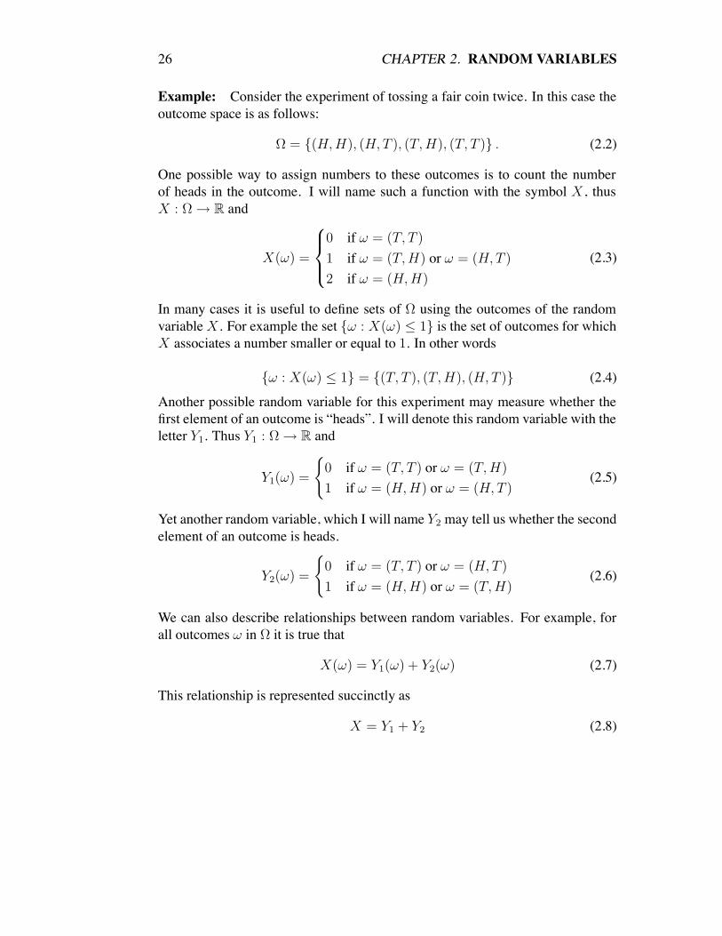
Example: Consider the experiment of tossing a fair coin twice. In this case theoutcome space is as follows:

! = {(H, H), (H, T ), (T, H), (T, T )} . (2.2)

One possible way to assign numbers to these outcomes is to count the numberof heads in the outcome. I will name such a function with the symbol X , thusX : ! ) R and

X(!) =

0 if ! = (T, T )

1 if ! = (T, H) or ! = (H, T )

2 if ! = (H, H)

(2.3)

In many cases it is useful to define sets of ! using the outcomes of the randomvariable X . For example the set {! : X(!) * 1} is the set of outcomes for whichX associates a number smaller or equal to 1. In other words

{! : X(!) * 1} = {(T, T ), (T, H), (H, T )} (2.4)

Another possible random variable for this experiment may measure whether thefirst element of an outcome is “heads”. I will denote this random variable with theletter Y1. Thus Y1 : ! ) R and

Y1(!) =

{0 if ! = (T, T ) or ! = (T, H)

1 if ! = (H, H) or ! = (H, T )(2.5)

Yet another random variable, which I will name Y2 may tell us whether the secondelement of an outcome is heads.

Y2(!) =

{0 if ! = (T, T ) or ! = (H, T )

1 if ! = (H, H) or ! = (T, H)(2.6)

We can also describe relationships between random variables. For example, forall outcomes ! in ! it is true that

X(!) = Y1(!) + Y2(!) (2.7)

This relationship is represented succinctly as

X = Y1 + Y2 (2.8)

27

Example: Consider an experiment in which we select a sample of 100 stu-dents from UCSD using simple random sampling (i.e., all the students have equalchance of being selected and the selection of each students does not constrain theselection of the rest of the students). In this case the sample space is the set ofall possible samples of 100 students. In other words, each outcome is a samplethat contains 100 students.1 A possible random variable for this experiment is theheight of the first student in an outcome (remember each outcome is a sample with100 students). We will refer to this random variable with the symbol H1. Notegiven an outcome of the experiment, (i.e., a sample of 100 students) H1 wouldassign a number to that outcome. Another random variable for this experimentis the height of the second student in an outcome. I will call this random vari-able H2. More generally we may define the random variables H1, . . . , H100 whereHi : ! ) R such that Hi(!) is the height of the subject number i in the sample !.The average height of that sample would also be a random variable, which couldbe symbolized as H and defined as follows

H(!) =1

100(H1(!) + · · ·+ H100(!)) for all ! ! ! (2.9)

or more succinctly

H =1

100(H1 + · · ·+ H100) (2.10)

I want you to remember that all these random variables are not numbers, theyare functions (rules) that assign numbers to outcomes. The output of these func-tions may change with the outcome, thus the name random variable.

Definition A random variable X on a probability space (!,F , P ) is a functionX : ! ) R. The domain of the function is the outcome space and the target isthe real numbers.2

Notation: By convention random variables are represented with capital letters.For example X : ! ) R, tells us that X is a random variable. Specific values of arandom variable are represented with small letters. For example, X(!) = u tells

1The number of possible outcomes is n!/(100! (n& 100)!) where n is the number of studentsat UCSD.

2Strictly speaking the function has to be Borel measurable (see Appendix), in practice thefunctions of interest to empirical scientists are Borel measurable so for the purposes of this bookwe will not worry about this condition.


us that the “measurement” assigned to the outcome ! by the random variable Xis u. Also I will represents sets like

{! : X(!) = u} (2.11)

with the simplified notation{X = u} (2.12)

I will also denote probabilities of such sets in a simplified, yet misleading, way.For example, the simplified notation

P (X = u) (2.13)

orP ({X = u}) (2.14)

will stand forP ({! : X(!) = u}) (2.15)

Note the simplified notation is a bit misleading since for example X cannot pos-sibly equal u since the first is a function and the second is a number.

Definitions:

• A random variable X is discrete if there is a countable set or real numbers{x1, x2, . . .} such that P (X ! {x1, x2, . . .}) = 1.

• A random variable X is continuous if for all real numbers u the probabilitythat X takes that value is zero. More formally, for all u ! R, P (X = u) =0.

• A random variable X ismixed if it is not continuous and it is not discrete.

2.1 Probability mass functions.A probability mass function is a function pX : R ) [0, 1] such that

pX(u) = P (X = u) for all u ! R. (2.16)

2.1. PROBABILITY MASS FUNCTIONS. 29

Note: If the random variable is continuous, then pX(u) = 0 for all values of u.Thus,

∑

u%RpX(u) =

0 if X is continuous1 if X is discreteneither 0 nor 1 if X is mixed

(2.17)

where the sum is done over the entire set of real numbers. What follows aresome important examples of discrete random variables and their probability massfunctions.

Discrete UniformRandom Variable: A random variable X is discrete uniformis there is a finite set of real numbers {x1, . . . , xn} such that

pX(u) =

{1/n if u ! {x1, . . . , xn}0 else

(2.18)

For example a uniform random variable that assigns probability 1/6 to the numbers{1, 2, 3, 4, 5, 6} and zero to all the other numbers could be used to model thebehavior of fair dies.

Bernoulli Random Variable: Perhaps the simplest random variable is the socalled Bernoulli random variable, with parameter µ ! [0, 1]. The Bernoulli ran-dom variable has the following probability mass function

pX(y) =

µ if y = 1

1 & µ if y = 0

0 if y "= 1 and y "= 0

(2.19)

For example, a Bernoulli random variable with parameter µ = 0.5 could be usedto model the behavior of a random die. Note such variable would also be discreteuniform.

Binomial RandomVariable: A random variable X is binomial with parametersµ ! [0, 1] and n ! N if its probability mass function is as follows

pX(y) =

{(ny

)µy(1 & µ)n#y if u ! {0, 1, 2, 3, . . .}

0 else(2.20)


Binomial probability mass functions are used to model the probability of obtainingy “heads” out of tossing a coin n times. The parameter µ represents the probabilityof getting heads in a single toss. For example if we want to get the probability ofgetting 9 heads out of 10 tosses of a fair coin, we set n = 10, µ = 0.5 (since thecoin is fair).

pX(9) =

(10

9

)(0.5)9(0.5)10#9 =

10!

9!(10 & 9)!(0.5)10 = 0.00976 (2.21)

Poisson Random Variable A random variable X is Poisson with parameter# > 0 if its probability mass function is as follows

pX(u) =

{!ue−λ

u! if u ( 0

0 else(2.22)

Poisson random variables model the behavior of random phenomena that occurwith uniform likelihood in space or in time. For example, suppose on averagea neuron spikes 6 times per 100 millisecond. If the neuron is Poisson then theprobability of observing 0 spikes in a 100 millisecond interval is as follows

pX(0) =60e#6

0!= 0.00247875217 (2.23)

2.2 Probability density functions.The probability density of a random variable X is a function fX : R ) R suchthat for all real numbers a > b the probability that X takes a value between a andb equals the area of the function under the interval [a, b]. In other words

P (X ! [a, b]) =

∫ b

a

fX(u)du (2.24)

Note if a random variable has a probability density function (pdf) then

P (X = u) =

∫ u

u

fX(x)dx = 0 for all values of u (2.25)

and thus the random variable is continuous.

2.2. PROBABILITY DENSITY FUNCTIONS. 31

Interpreting probability densities: If we take an interval very small the areaunder the interval can be approximated as a rectangle, thus, for small "x

P (X ! (x, x + "x]) + fX(x)"x (2.26)

fX(u) + P (X ! (x, x + "x])

"x(2.27)

Thus the probability density at a point can be seen as the amount of probabilityper unit length of a small interval about that point. It is a ratio between two dif-ferent ways of measuring a small interval: The probability measure of the intervaland the length (also called Lebesgue measure) of the interval. What follows areexamples of important continuous random variables and their probability densityfunctions.

Continuous Uniform Variables: A random variable X is continuous uniformin the interval [a, b], where a and b are real numbers such that b > a, if its pdf isas follows;

fX(u) =

{1/(b & a) if u ! [a, b]

0 else(2.28)

Note how a probability density function can take values larger than 1. For exam-ple, a uniform random variable in the interval [0, 0.1] takes value 10 inside thatinterval and 0 everywhere else.

Continuous Exponential Variables: A random variable X is called exponen-tial if it has the following pdf

fX(u) =

{0 if u < 0

# exp(&#x) if u ( 0(2.29)

we can calculate the probability of the interval [1, 2] by integration

P ({X ! [1, 2]}) =

∫ 2

1

# exp(&#x)dx =[& exp(&#x)

]2

1(2.30)

if # = 1 this probability equals exp(&1) & exp(&2) = 0.2325.


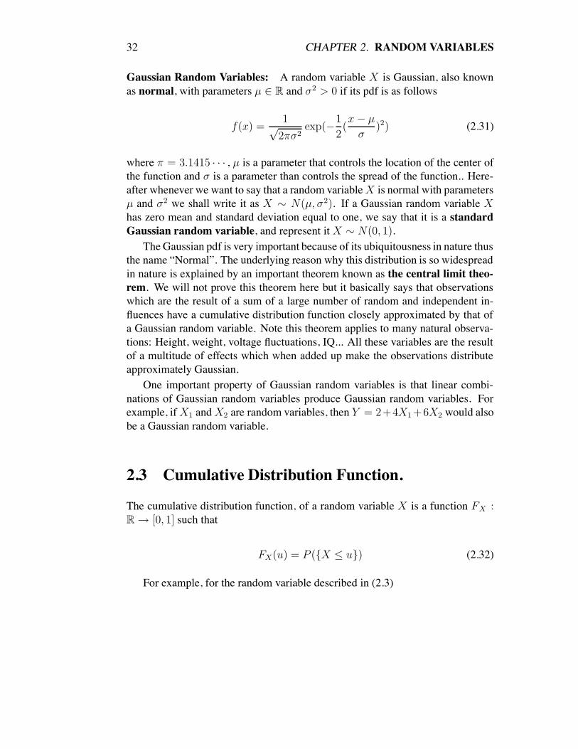
Gaussian Random Variables: A random variable X is Gaussian, also knownas normal, with parameters µ ! R and $2 > 0 if its pdf is as follows

f(x) =1'

2"$2exp(&1

2(x & µ

$)2) (2.31)

where " = 3.1415 · · · , µ is a parameter that controls the location of the center ofthe function and $ is a parameter than controls the spread of the function.. Here-after whenever we want to say that a random variable X is normal with parametersµ and $2 we shall write it as X , N(µ, $2). If a Gaussian random variable Xhas zero mean and standard deviation equal to one, we say that it is a standardGaussian random variable, and represent it X , N(0, 1).

The Gaussian pdf is very important because of its ubiquitousness in nature thusthe name “Normal”. The underlying reason why this distribution is so widespreadin nature is explained by an important theorem known as the central limit theo-rem. We will not prove this theorem here but it basically says that observationswhich are the result of a sum of a large number of random and independent in-fluences have a cumulative distribution function closely approximated by that ofa Gaussian random variable. Note this theorem applies to many natural observa-tions: Height, weight, voltage fluctuations, IQ... All these variables are the resultof a multitude of effects which when added up make the observations distributeapproximately Gaussian.

One important property of Gaussian random variables is that linear combi-nations of Gaussian random variables produce Gaussian random variables. Forexample, if X1 and X2 are random variables, then Y = 2+4X1 +6X2 would alsobe a Gaussian random variable.

2.3 Cumulative Distribution Function.

The cumulative distribution function, of a random variable X is a function FX :R ) [0, 1] such that

FX(u) = P ({X * u}) (2.32)

For example, for the random variable described in (2.3)

2.3. CUMULATIVE DISTRIBUTION FUNCTION. 33

FX(u) =

0.0 if u < 0.0

1/4 if u ( 0.0 and u < 1

3/4 if u ( 1 and u < 2

1.0 if u ( 2

(2.33)

The relationship between the cumulative distribution function, the probabilitymass function and the probability density function is as follows:

FX(u) =

{∑x&u pX(u) if X is a discrete random variable∫ u

#" fX(x)dx if X is a continuous random variable(2.34)

Example: To calculate the cumulative distribution function of a continuous ex-ponential random variable X with parameter # > 0 we integrate the exponentialpdf

FX(u) =

{∫ u

0 # exp(&#x)dx if u ( 0

0 else(2.35)

And solving the integral∫ u

0

# exp(&#x)dx =

[& exp(&#x)

]u

0

= 1 & exp(&#u) (2.36)

Thus the cumulative distribution of an exponential random variable is as follows

FX(u) =

{1 & exp(&#u) if u ( 0

0 else(2.37)

Observation: We have seen that if a random variable has a probability den-sity function then the cumulative density function can be obtained by integration.Conversely we can differentiate the cumulative distribution function to obtain theprobability density function

fX(u) =dFX(u)

du(2.38)


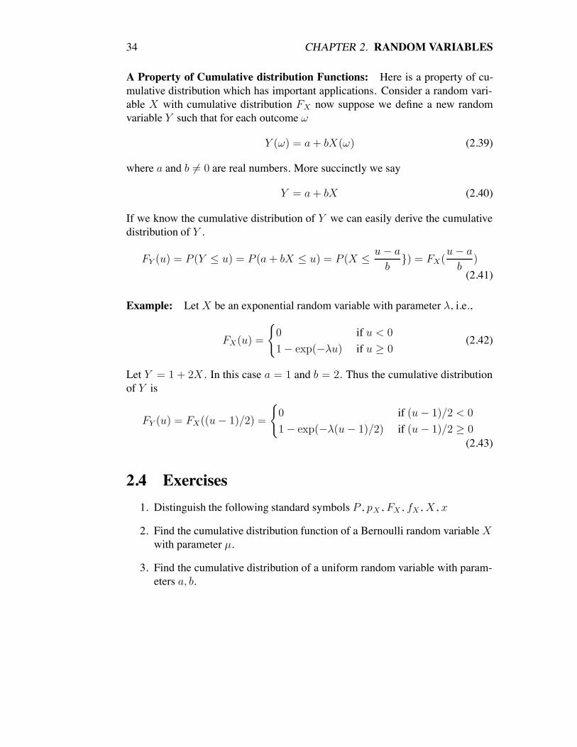
A Property of Cumulative distribution Functions: Here is a property of cu-mulative distribution which has important applications. Consider a random vari-able X with cumulative distribution FX now suppose we define a new randomvariable Y such that for each outcome !

Y (!) = a + bX(!) (2.39)

where a and b "= 0 are real numbers. More succinctly we say

Y = a + bX (2.40)

If we know the cumulative distribution of Y we can easily derive the cumulativedistribution of Y .

FY (u) = P (Y * u) = P (a + bX * u) = P (X * u & a

b}) = FX(

u & a

b)

(2.41)

Example: Let X be an exponential random variable with parameter #, i.e.,

FX(u) =

{0 if u < 0

1 & exp(&#u) if u ( 0(2.42)

Let Y = 1 + 2X . In this case a = 1 and b = 2. Thus the cumulative distributionof Y is

FY (u) = FX((u & 1)/2) =

{0 if (u & 1)/2 < 0

1 & exp(&#(u & 1)/2) if (u & 1)/2 ( 0(2.43)

2.4 Exercises1. Distinguish the following standard symbols P , pX , FX , fX , X , x

2. Find the cumulative distribution function of a Bernoulli random variable Xwith parameter µ.

3. Find the cumulative distribution of a uniform random variable with param-eters a, b.

2.4. EXERCISES 35

4. Consider a uniform random variable in the interval [0, 1].

(a) Calculate the probability of the interval [0.1, 0.2]

(b) Calculate the probability of 0.5.

5. Let X be a random variable with probability mass function

pX(u) =

{1/5 if u ! {1, 2, 3, 4, 5}0 else

(2.44)

(a) Find FX(4)

(b) Find P ({X * 3} % {X * 4})(c) Plot the function hX(t) = P ({X = t} | {X ( t}) for t = 1, 2, 3, 4, 5.

This function is commonly known as the “hazard function” of X . Ifyou think of X as the life time of a system, hX(t) tells us the proba-bility that the system fails at time t given that it has not failed up totime t. For example, the hazard function of human beings looks likea U curve with a extra bump at the teen-years and with a minimum atabout 30 years.

6. Let X be a continuous random variable with pdf

fX(u) =

0.25 if u ! [&3,&1]

0.25 if u ! [1, 3]

0 else(2.45)

(a) Plot fX . Can it be a probability density function? Justify your re-sponse.

(b) Plot FX

7. Show that if X is a continuous random variable with pdf fX and Y = a+bXwhere and a, b are real numbers. Then

fY (v) = (1/b)fX(u & a

b) (2.46)

hint: Work with cumulative distributions and then differentiate them to getdensities.

8. Show that if X , N(µ, $2) then Y = a + bX is Gaussian.


Chapter 3

Random Vectors

In many occasions we need to model the joint behavior of more than one variable.For example, we may want to describe whether two different stocks tend to fluc-tuate in a somewhat linked manner or whether high levels of smoking covary withhigh lung cancer rates. In this chapter we examine the joint behavior of more thanone random variables. To begin with, we will start working with pairs of randomvariables.

3.1 Joint probability mass functionsThe joint probability mass function of the random variables X and Y is a functionpX,Y : R2 ) [0, 1], such that for all (u, v) ! R2

pX,Y (u, v) = P ({X = u} % {Y = v}) (3.1)

hereafter, we use the simplified notation P (X = u, Y = u) to represent P ({X =u} % {Y = v}), i.e., the probability measure of the set

{! : (X(!) = u)and(Y (!) = v)} (3.2)

3.2 Joint probability density functionsThe joint probability density function of the continuous random variables X andY is a function fX,Y : R2 ) [0,-) such that for all (u, v) ! R2 and for all

37

38 CHAPTER 3. RANDOM VECTORS

("u, "v) ! R2

P (X ! [u, u + "u], Y ! [v, v + "v]) =

∫ u+!u

u

∫ v+!v

v

fX,Y (u, v) dv du (3.3)

Interpretation Note if "u and "v are so small that fX,Y (u, v) is approximatelyconstant over the area of integration then

P (X ! [u, u + "u], Y ! [v, v + "v]) + fX,Y (u, v)"u "v (3.4)

In other words, the probability that (X, Y ) take values in the rectangle [u, u +"u] . [v, v + "v] is approximately the area of the rectangle times the density ata point in the rectangle.

3.3 Joint Cumulative Distribution FunctionsThe joint cumulative distribution of two random variables X and Y is a functionFX,Y : R2 ) [0, 1] such that

FX,Y (u, v) = P ({X * u} % {Y * v}) (3.5)

note if X and Y are discrete then

FX,Y (u, v) =∑

x&u

∑

y&v

pX,Y (u, v) (3.6)

and if X and Y are continuous then

FX,Y (u, v) =

∫ u

#"

∫ v

#"fX,Y (u, v) dv du (3.7)

3.4 MarginalizingIn many occasions we know the joint probability density or probability mass func-tion of two random variables X and Y and we want to get the probability den-sity/mass of each of the variables in isolation. Such a process is called marginal-ization and it works as follows:

pX(u) =∑

v%RpX,Y (u, v) (3.8)

3.5. INDEPENDENCE 39

and if the random variables are continuous

fX(u) =

∫ "

#"fX,Y (u, v) dv (3.9)

Proof: Consider the function h : R ) R

h(u) =

∫ "

#"fX,Y (u, v) dv (3.10)

We want to show that h is the probability density function of X . Note for alla, b ! R such that a * b

P (X ! [a, b]) = P (X ! [a, b], Y ! R) =

∫ b

a

fX,Y (u, v) dv du =

∫ b

a

h(u) du

(3.11)showing that h is indeed the probability density function of X . A similar argumentcan be made for the discrete case.

3.5 IndependenceIntuitively, two random variables X and Y are independent if knowledge aboutone of the variables gives us no information whatsoever about the other variable.More precisely, the random variables X and Y are independent if and only if allevents of the form {X ! [u, u+"u]} and all events of the form {Y ! [v, v+"v]}are independent. If the random variable is continuous, a necessary and sufficientcondition for independence is that the joint probability density be the product ofthe densities of each variable

fX,Y (u, v) = fX(u)fY (v) (3.12)

for all u, v ! R. If the random variable is discrete, a necessary and sufficient con-dition for independence is that the joint probability mass function be the productof the probability mass for each of the variables

pX,Y (u, v) = pX(u)pY (v) (3.13)

for all u, v ! R.


3.6 Bayes’ Rule for continuous data and discrete hy-potheses

Perhaps the most common application of Bayes’ rule occurs when the data arerepresented by a continuous random variable X , and the hypotheses by a discreterandom variable H . In such case, Bayes’ rule works as follows

pH|X(i | u) =fX|H(u|i) pH(i)

fX(u)(3.14)

where pH|X : R2 ) [0, 1] is known as the conditional probability mass functionof H given X and it is defined as follows

pH|X(i | u) = lim!u!0

P (H = i | X ! [u, u + "u]) (3.15)

fX|H : R2 ) R+ is known as the conditional probability density function of Xgiven H and it is defined as follows: For all a, b ! R such that a * b,

P (X ! [a, b] | H = i) =

∫ b

a

fX|H(u|i) du (3.16)

Proof: Applying Bayes’ rule to the events {H = i} and {X ! [u, u + "u]}

P (H = i | X ! [u, u + "u]) =P (X ! [u, u + "u] | H = i) P (H = i)

P (X ! [u, u + "u])(3.17)

=

∫ u+!u

u fX|H(x|i) dx P (H = i)∫ u+!u

u fX(x) dx(3.18)

Taking limits and approximating areas with rectangles

lim!u!0

P (H = i | X ! [u, u + "u]) ="ufX|H(u|i)pH(i)

"ufX(u)(3.19)

The "u terms cancel out, completing the proof.

3.6. BAYES’ RULE FOR CONTINUOUS DATA AND DISCRETE HYPOTHESES41

3.6.1 A useful version of the LTPIn many cases we are not given fX directly and we need to compute it usingfX|H and pH . This can be done using the following version of the law of totalprobability:

fX(u) =∑

j%Range(H)

pH(j) fX|H(u|j) (3.20)

Proof: Note that for all a, b ! R, with a * b∫ b

a

∑

j%Range(H)

pH(j)fX|H(u|j) du =∑

j%Range(H)

pH(j)

∫ b

a

fX|H(u|j) du (3.21)

=∑

j%Range(H)

pH(j)P (X ! [a, b] | H = j) = P (X ! [a, b]) (3.22)

and thus∑

j%Range(H) pH(j)fX|H(u|j) is the probability density of X .

Example: Let H be a Bernoulli random variable with parameter µ = 0.5. LetY0 , N(0, 1), Y1 , N(1, 1) and

X = (1 & H)(Y0) + (H)(Y1) (3.23)

Thus,

pH(0) = pH(1) = 0.5 (3.24)

fX|H(u | i) =1'2"

e#(u#i)2/2 for i ! {1, 2}. (3.25)

Suppose we are given the value u ! R and we want to know the posterior prob-ability that H takes the value 0 given that X took the value u. To do so, first weapply LTP to compute fX(u)

fX(u) = (0.5)1'2"

(e#u2/2 +e#(u#1)2/2

)= (0.5)

1'2"

eu2/2

(1+e2u#1

)(3.26)

Applying Bayes’ rule,

pH|X(0 | u) =1

1 + e#(1#2u)(3.27)

So, for example, if u = 0.5 the probability that H takes the value 0 is 0.5. If u = 1the probability that H takes the value 0 drops down to 0.269.


3.7 Random Vectors and Stochastic ProcessesA random vector is a collection of random variables organized as a vector. Forexample if X1, . . . , Xn are random variables then

X = (X1, Y, . . . , Xn)$ (3.28)

is a random vector. A stochastic process is an ordered set of random vectors. Forexample, if I is an indexing set and Xt, is a random vector for all t ! I then

X = (Xi : i ! I) (3.29)

is a random process. When the indexing set is countable, Y is called a “discretetime” stochastic process. For example,

X = (X1, Y, X3, . . .) (3.30)

is a discrete time random process. If the indexing set are the real numbers, thenY is called a “continuous time” stochastic process. For example, if X is a randomvariable, the ordered set of random vectors

X = (Xt : t ! R) (3.31)

withXt(!) = sin(2"tX(!)) (3.32)

is a continuous time stochastic process.

Chapter 4

Expected Values

The expected value (or mean) of a random variable is a generalization of the notionof arithmetic mean. It is a number that tells us about the “center of gravity” oraverage value we would expect to obtain is we averaged a very large numberof observations from that random variable. The expected value of the randomvariable X is represented as E(X) or with the Greek letter µ, as in µX and it isdefined as follows

E(X) = µX =

{∑u%R pX(u)u for discrete ravs∫ +"

#" pX(u)u du for continuous ravs(4.1)

We also define the expected value of a number as the number itself, i.e., for allu ! R

E(u) = u (4.2)

Example: The expected value of a Bernoulli random variable with parameter µis as follows

E(X) = (1 & µ)(0.0) + (µ)(1.0) = µ (4.3)

Example: A random variable X with the following pdf

pX(u) =

{1

b#a if u ! [a, b]

0 if u "! [a, b](4.4)

43

44 CHAPTER 4. EXPECTED VALUES

is known as a uniform [0, 1] continuous random variable. Its expected value is asfollows

E(X) =

∫ "

#"pX(u)u du =

∫ b

a

1

b & au du

=1

(b & a)

[u2

2

]b

a=

=1

(b & a)(b2 & a2

2) = (a + b)/2 (4.5)

Example: The expected value of an exponential random variable with param-eter #is as follows (see previous chapter for definition of an exponential randomvariable)

E(X) =

∫ "

#"upX(u)du =

∫ "

0

u# exp(&#u)du (4.6)

and using integration by parts

E(X) =[& u exp(&#u)

]"0

+

∫ "

0

# exp(&#u)du = &[# exp(&#u)

]"0

=1

#(4.7)

4.1 Fundamental Theorem of Expected ValuesThis theorem is very useful when we have a random variable Y which is a functionof another random variable X . In many cases we may know the probability massfunction, or density function, for X but not for Y . The fundamental theorem ofexpected values allows us to get the expected value of Y even though we do notknow the probability distribution of Y . First we’ll see a simple version of thetheorem and then we will see a more general version.

Simple Version of the Fundamental Theorem: Let X : ! ) R be a rav andh : R ) R a function. Let Y be a rav defined as follows:

Y (!) = h(X(!)) for all ! ! R (4.8)

or more succinctlyY = h(X) (4.9)

4.1. FUNDAMENTAL THEOREM OF EXPECTED VALUES 45

Then it can be shown that

E(Y ) =

{∑u%R pX(u)h(u) for discrete ravs∫ +"

#" pX(u)h(u) du for continuous ravs(4.10)

Example: Let X be a Bernoulli rav and Y a random variable defined as Y =(X&0.5)2. To find the expected value of Y we can apply the fundamental theoremof expected values with h(u) = (u & 0.5)2. Thus,

E(Y ) =∑

u%RpX(u)(u & 0.5)2 = pX(0)(0 & 0.5)2 + pX(1)(1 & 0.5)2

= (0.5)(0.5)2 + (0.5)(&0.5)2 = 0.25 (4.11)

Example: The average entropy, or information value (in bits) of a random vari-able X is represented as H(X) and is defined as follows

H(X) = &E(log2 pX(X)) (4.12)

To find the entropy of a Bernoulli random variable X with parameter µ we canapply the fundamental theorem of expected values using the function h(u) =log2 pX(u) . Thus,

H(X) =∑

u%RpX(u) log2 pX(u) = pX(0) log2 pX(0) + pX(1) log2 pX(1)

= (µ) log2(µ) + (1 & µ) log2(1 & µ) (4.13)

For example, if µ = 0.5, then

H(X) = (0.5) log2(0.5) + (0.5) log2(0.5) = 1 bit (4.14)

General Version of the Fundamental Theorem: Let X1, . . . , Xn be randomvariables, let Y = h(X1, . . . , Xn), where h : Rn ) R is a function. Then

E(Y ) =

{∑(u1, . . . , un) ! RnpX1,...,Xn(u1, . . . , un)h(u1, . . . , un) for discrete ravs∫ +"

#" · · ·∫ +"#" pX1,...,Xn(u1, . . . , un)h(u1, . . . , un)du1 · · · dun for continuous ravs

(4.15)


4.2 Properties of Expected ValuesLet X and Y be two random variables and a and b two real numbers. Then

E(X + Y ) = E(X) + E(Y ) (4.16)and

E(a + bX) = a + bE(X) (4.17)Moreover if X and Y are independent then

E(XY ) = E(X)E(Y ) (4.18)We will prove these properties using discrete ravs. The proofs are analogous forcontinuous ravs but substituting sums by integrals.

Proof: By the fundamental theorem of expected values

E(X + Y ) =∑

u%R

∑

v%RpX,Y (u, v)(u + v)

= (∑

u%Ru

∑

v%RpX,Y (u, v)) + (

∑

v%Rv

∑

u%RpX,Y (u, v))

=∑

u%R

upX(u) +∑

v%RvpY (v) = E(X) + E(Y ) (4.19)

where we used the law of total probability in the last step.

Proof: Using the fundamental theorem of expected values

E(a + bX) =∑

u

pX(u)(a + bu)

= a∑

u%RpX(u) + b

∑

u

upX(u) = a + bE(X) (4.20)

Proof: By the fundamental theorem of expected values

E(XY ) =∑

u%R

∑

v%RpX,Y (u, v)uv (4.21)

if X and Y are independent then pX,Y (u, v) = pX(u)pY (v). Thus

E(XY ) = [∑

u

upX(u)] [∑

v

vpY (v)] = E(X)E(Y ) (4.22)

!

4.3. VARIANCE 47

4.3 VarianceThe variance of a random variable X is a number that represents the amountof variability in that random variable. It is defined as the expected value of thesquared deviations from the mean of the random variable and it is represented asVar(X) or as $2

X

Var(X) = $2X = E[(X&µX)2] =

{∑u%R pX(u)(u & µX)2 for discrete ravs∫ +"

#" pX(u)(u & µX)2du for continuous ravs(4.23)

The standard deviation of a random variable X is represented as Sd(X) or $ andit is the square root of the variance of that random variable

Sd(X) = $X =√

Var(X) (4.24)

The standard deviation is easier to interpret than the variance for it uses the sameunits of measurement taken by the random variable. For example if the randomvariable X represents reaction time in seconds, then the variance is measuredin seconds squares, which is hard to interpret, while the standard deviation ismeasured in seconds. The standard deviation can be interpreted as a “typical”deviation from the mean. If an observation deviates from the mean by about onestandard deviation, we say that that amount of deviation is “standard”.

Example: The variance of a Bernoulli random variable with parameter µ is asfollows

Var(X) = (1 & µ)(0.0 & µ)2 + (µ)(1.0 & µ)2 = (µ)(1 & µ) (4.25)

Example: For a continuous uniform [a, b] random variable X , the pdf is as fol-lows

pX(u) =

{1

b#a if u ! [a, b]

0 if u "! [a, b](4.26)

which we have seen as expected value µX = (a + b)/2. Its variance is as follows

$2X =

∫ +"

#"upX(u)du =

1

b & a

∫ b

a

(u & (a + b)/2)2du (4.27)


and doing a change of variables y = (u & (a + b)/2)

$2X =

1

b & a

∫ (b#a)/2

(a#b)/2

y2dy =1

b & a

[y3/3

](b#a)/2

(a#b)/2=

b & a

12(4.28)

Exercise: We will show that in a Gaussian random variable the parameter µ isthe mean and $ the standard deviation. First note

E(X) =

∫ "

#"u

1'2"$2

exp(&1

2(u & µ

$)2)du (4.29)

changing to the variable y = (u & µ)

E(X) =1'

2"$2

∫ "

#"y exp(&1

2(y

$)2)dy

+ µ[1'

2"$2

∫ "

#"exp(&1

2(y

$)2)] = µ (4.30)

The first term is zero because the integrand is an odd function (i.e., g(&x) =&g(x). For the variance

Var(X) =1'

2"$2

∫ "

#"(u & µ)2 exp(&1

2(u & µ

$)2)du (4.31)

changing variables to y = (u & µ)

Var(X) =1'

2"$2

∫ "

#"y y exp(&1

2(y

$)2)dy (4.32)

and using integration by parts

Var(X) =1'

2"$2

(& $2

[y exp(&1

2(y/$)2)

]+"

#"

+ $2

∫ "

#"exp(&1

2(y

$)2)dy

)= $2 (4.33)

4.3.1 Properties of the VarianceLet X and Y be two random variables and a and b two real numbers then

Var(aX + b) = a2Var(X) (4.34)

4.3. VARIANCE 49

andVar(X + Y ) = Var(X) + Var(Y ) + 2Cov(X, Y ) (4.35)

where Cov(X, Y ) is known as the covariance between X and Y and is defined as

Cov(X, Y ) = E[(X & E(X))(Y & E(Y ))] (4.36)

Proof:

Var(aX + b) = E[(aX + b & E(aX + b))2] = E[(aX + b & aE(X) & b)2]

= E[(a(X & E(X))2] = a2E[(X & E(X))2] = a2Var(X) (4.37)

Proof:

Var(X + Y ) = E(X + Y & E(X + Y ))2 = E((X & µX) + (Y & µY ))2

= E[(X & µX)2] + E[(Y & µY )2] + 2E[(X & µX)(Y & µY )] (4.38)

!

If Cov(X, Y ) = 0 we say that the random variables X and Y are uncorrelated.In such case the variance of the sum of the two random variables equals the sumof their variances.

It is easy to show that if two random variables are independent they are alsouncorrelated. To see why note that

Cov(X, Y ) = E[(X&µX)(Y & µY )] = E(XY ) & µY E(X) (4.39)& µXE(Y ) + µXµY = E(XY ) & E(X)E(Y ) (4.40)

we have already seen that if X and Y are independent then E(XY ) = E(X)E(Y )and thus X and Y are uncorrelated.

However two random variables may be uncorrelated and still be dependent.Think of correlation as a linear form of dependency. If two variables are uncor-related it means that we cannot use one of the variables to linearly predict theother variable. However in uncorrelated variables there may still be non-linearrelationships that make the two variables non-independent.


Example: Let X, Y be random variables with the following joint pmf

pX,Y (u, v) =

1/3 if u = &1 and v = 1

1/3 if u = 0 and v = 0

1/3 if u = 1 and v = 1

0 else

(4.41)

show that X and Y are uncorrelated but are not independent.

Answer: Using the fundamental theorem of expected values we can computeE(XY )

E(XY ) = (1/3)(&1)(1) + (1/3)(0)(0) + (1/3)(1)(1) = 0 (4.42)

From the joint pmf of X and Y we can marginalize to obtain the pmf of X and ofY

pX(u) =

1/3 if u = &1

1/3 if u = 0

1/3 if u = 1

0 else

(4.43)

pY (v) =

1/3 if v = 0

2/3 if v = 1

0 else(4.44)

Thus

E(X) = (1/3)(&1) + (1/3)(0) + (1/3)(1) = 0 (4.45)E(Y ) = (1/3)(0) + (2/3)(1) = 2/3 (4.46)Cov(X, Y ) = E(XY ) & E(X)E(Y ) = 0 & (0)(2/3) = 0 (4.47)

Thus X and Y are uncorrelated. To show that X and Y are not independent notethat

pX,Y (0, 0) = 1/3 "= pX(0)pY (0) = (1/3)(1/3) (4.48)

4.4. APPENDIX: USING STANDARD GAUSSIAN TABLES 51

4.4 Appendix: Using Standard Gaussian TablesMost statistics books have tables for the cumulative distribution of Gaussian ran-dom variables with mean µ = 0 and standard deviation $ = 1. Such a cumulativedistribution is known as the standard Gaussian cumulative distribution and it isrepresented with the capital Greek letter “Phi”, i.e., #. So #(u) is the probabilitythat a standard Gaussian random variable takes values smaller or equal to u. Inmany cases we need to know the probability distribution of a Gaussian randomvariable X with mean µ different from zero and variance $2 different from 1. Todo so we can use the following trick

FX(u) = #(x & µ

$) (4.49)

For example, the probability that a Gaussian random variable with mean µ = 2and standard deviation $ = 4 takes values smaller than 6 can be obtained asfollows

P (X * 6) = FX(6) = #(6 & 2

4) = #(1) (4.50)

If we go to the standard Gaussian tables we see that #(1) = 0.8413.

Proof: Let Z be a standard Gaussian random variable, and X = µ + $Z. Thus,

E(X) = µ + E(Z) = µ (4.51)

Var(X) = $2Var(Z) = $2 (4.52)

Thus, X has the desired mean and variance. Moreover since X is a linear transfor-mation of Z then X is also Gaussian. Now, using the the properties of cumulativedistributions that we saw in a previous chapter

FX(u) = FZ((u & µ)/$) = #((u & µ)/$)) (4.53)

!

Example: Let Y be a Gaussian rav with µY = 10 and $2Y = 100. Suppose we

want to compute FY (&20). First we compute z = (&20 & µY )/$Y = &1. Wego to the standard Gaussian tables and find FZ(&1) = 0.1587 Thus FY (20) =FZ(&1) = 0.1587.


4.5 Exercises1. Let a random variable X represent the numeric outcome of rolling a fair

die, i.e., pX(u) = 1/6 for u ! {1, 2, 3, 4, 5, 6}. Find the expected value ,standard deviation, and average information value of X .

2. Consider the experiment of tossing a fair coin twice. Let X1 be a randomvariable taking value 1 if the first toss is heads, and 0 otherwise. Let X2 bea random variable taking value 1 if the second toss is heads, and 0 else.

(a) Find E(X1), E(X2)

(b) Find Var(X1), Var(X2)

(c) Find Var(X1/2) and Var(X2/2)

(d) Find Var(X1 + X2) and Var[(X1 + X2)/2]

3. Find the information value of a continuous random variable in the interval[a, b].

4. Show that the variance of an exponential random variable with parameter #is 1/#2.

5. Let X be a standard Gaussian random variable. Using Gaussian tables find:

(a) FX(&1.0)

(b) FX(1.0)

(c) P (&1.0 * X * 1.0)

(d) P (X = 1.0)

Chapter 5

The precision of the arithmetic mean

Consider taking the average of a number of observations all of which are ran-domly sampled from a large population. Intuitively it seems that as the numberof observations increases this average will get closer and closer to the true popu-lation mean. In this chapter we quantify how close the sample mean gets to thepopulation mean as the number of observations in the sample increases. In otherwords we want to know how good the mean of a sample of noisy observations isas an estimate of the “true” value underlying those observations.

Let’s formalize the problem using our knowledge of probability theory. Westart with n independent random variables variables X1, . . . , Xn. We will also as-sume that all these random variables have the same mean, which we will representas µ and the same variance, which we will represent as $2. In other words

E(X1) = E(X2) = · · · = E(Xn) = µ (5.1)

andVar(X1) = Var(X2) = · · · = Var(Xn) = $2 (5.2)

This situation may occur, when our experiment consists of randomly selecting nindividuals from a population (e.g., 20 students from UCSD). In this case the out-comes of the random experiment consists of a sample of n subjects. The outcomespace is the set of all possible samples of n subjects. The random variable Xi

would represent a measurement of subject number i in the sample. Note that inthis case all random variables have the same mean, which would be equal to theaverage observation for the entire population. They also have the same variance,since all subjects have an equal chance of being in any of the n possible positionsof the samples.

53

54 CHAPTER 5. THE PRECISION OF THE ARITHMETIC MEAN

Given a sample ! we can average the n values taken by the random variablesfor that particular sample. We will represent this average as Xn,

Xn(!) =1

n

n∑

i=1

Xi(!); for all ! ! ! (5.3)

More concisely,

Xn =1

n

n∑

i=1

Xi (5.4)

Note that Xn is itself a random variable (i.e., a function from the outcome spaceto the real numbers). We call this random variable the sample mean.

One convenient way to measure the precision of the sample mean is to com-pute the expected squared deviation of the sample mean from the true populationmean, i.e., √

E[(Xn & µ)2] (5.5)

For example, if√

E[(Xn & µY )2] = 4.0secs this would tell us that on average thesample mean deviates from the population mean by about 4.0 secs.

5.1 The sampling distribution of the meanWe can now use the properties of expected values and variances to derive theexpected value and variance of the sample mean .

E(Xn) =1

n

n∑

i=1

E(Xi) = µ (5.6)

thus the expected value of the sample mean is the actual population mean of therandom variables. A consequence of this is that

E[(Xn & µ)2] = E[(Xn & E(Xn))2] = Var(Xn) (5.7)

This takes us directly to our goal. Using the properties of the variance, and con-sidering that the random variables X1, . . . , Xn are independent we get

V ar(Xn) =1

n2

n∑

i=1

Var(Xi) =$2

n(5.8)

5.1. THE SAMPLING DISTRIBUTION OF THE MEAN 55

The standard deviation of the mean is easier to interpret than the variance of themean. It roughly represents how much the means of independent randomly ob-tained samples typically differ from the population mean. Since the standard de-viation of the mean is so important, many statisticians give it a special name: thestandard error of the mean. Thus the standard error of the mean simply is thesquare root of the variance of the mean, and it is represented as Sd(Xn) or Se(Xn).Thus,

Sd(Xn) =$'n

=√

E[(Xn & µ)2] (5.9)

Finally we are done! Equation 5.9 tells us that the uncertainty of the samplemean (its standard deviation) increases proportionally to the uncertainty aboutindividual observations ($) and decreases proportionally to the square root of thenumber of observations. Thus, if we want to double the precision of the samplemean (reduce its standard deviation by half) we need to quadruple the number ofobservations in the sample.

Example: Let X1 and X2 be independent Bernoulli random variables with pa-rameter µ = 0.5. Thus E(X1) = E(X2) = µ = 0.5 and Var(X1) = Var(X2) =$2 = 0.25, moreover

E(X2) = (0)(0.25) + (0.5)(0.5) + (1)(0.25) = 0.5 = µ (5.10)

Var(X2) = $2/2 = 0.125 (5.11)

5.1.1 Central Limit TheoremThis is a very important theorem which we will not prove here. The theorem tellsus that as n goes to infinity, the cumulative distribution of Xn is closely approx-imated by that of a Gaussian random variable with mean E(Xn) and standarddeviation Sd(Xn). In practice for n ( 30 the Gaussian cumulative distributionprovides very good approximations.

Example: We toss a fair coin 100 times. What is the probability that the pro-portion of “heads” be smaller or equal to 0.45?

Answer: Tossing a fair coin 100 times can be modeled using 100 independentidentically distributed Bernoulli random variables each of which has parameter


µ = 0.5. Let’s represent these 100 random variables as X1, . . . , X100 where Xi

takes the value 1 if the ith time we toss the coin we get heads. Thus the proportionof heads is the average of the 100 random variables, we will represent it as X .

X =1

100(X1 + · · · + X100) (5.12)

We knowµ = E(X1) = · · · = E(X100) = 0.5 (5.13)

$2 = Var(X1) = · · · = Var(X100) = 0.25 (5.14)Thus

E(X) = 0.5 (5.15)Var(X) = $2/100 = 0.0025 (5.16)

Since n = 100 > 30 the cumulative distribution of X is approximately Gaussian.Thus

P (X * 0.45) = FX(0.45) + #(0.45 & 0.5'

0.0025) = #(&1) = 0.1586 (5.17)

5.2 Exercises1. The Central Limit Theorem

(a) Goto the book Web site and click on LinuStats ) Coin Simulator(b) Do 1000 replications of a coin tossing experiment. Each experiment

should consists of 10 coin tosses (10 observations per experiment).The result should be 1000 numbers each of which represents the pro-portion of tails obtained in a particular experiment. If we encodedHeads as “0” and tails as “1”, the outcome of a coin toss is an outcomefrom a Bernoulli 0,1 random variable with parameter µ = 0.5. Theproportion of tails obtained in 10 tosses is the average of 10 indepen-dent identically distributed Bernoulli random variables.

X =

∑10i=1 Xi

10(5.18)

This average is itself a random variable. Moreover the central limittheorem tell us that it should be approximately Gaussian. We willcheck that now:

5.2. EXERCISES 57

(c) Use the Edit menu in your browser to copy the 1000 numbers obtainedin the coin tossing experiments.

(d) Go back to LinuStats and choose the descriptive statistics page.(e) Use the Edit menu in your browser to paste the 1000 numbers into the

data window.(f) Choose a minimum value of 0, maximum value of 1, and window of

0.1(g) Analyze the data by clicking the appropriate button.(h) Copy the resulting relative frequency table and transform it into a cu-

mulative distribution function(i) Copy the Mean and SD (Standard Deviation) of the 1000 numbers.

Explain what this standard deviation means. I’ll call these numbersµX and $X

(j) Compare the obtained cumulative distribution function with that pre-dicted by a Gaussian distribution with mean µX and standard deviation$X .

2. The sampling distribution of the mean

(a) Go to the coin simulator and do 1000 experiments each with 1 toss(i.e., one observation per experiment). Using the same procedure asin the previous exercise, calculate the mean and standard deviation ofthe 1000 experiments. Plot the relative frequency density polygon.Interpret your results.

(b) Same as the previous question but now toss the coin 2 times per exper-iment. Obtain the new mean and standard deviation and interpret whatthey mean.

(c) Same with 4, 16 and with 32 observations per experiment.(d) Plot a graph with the obtained means as a function of the number of

tosses.(e) Plot a graph with the obtained standard deviations as a function of the

number of tosses.(f) Plot a graph with the obtained variances as a function of the number

of tosses.


(g) Explain your results. How does the mean, variance, and standard devi-ation change as the number of observations per experiment increases.How does the relative frequency density polygon change as the num-ber of observations per experiment increases? Does it make sense?

3. What is less probable: 1) to get 80 or more tails out of tossing a fair coin 100times, 2) to get 30 or more tails out of tossing a fair coin 50 times. NOTE:Since n > 30 you can assume that the cumulative distribution of the meanis approximately Gaussian.

4. An experimenter inserts intracellular electrodes on a large sample of ran-domly selected neurons in primary visual cortex (V1). Intracellular elec-trodes are designed to measure the response of single neurons. The re-searcher finds the average response of the neurons is 10 mVolts and thestandard deviation 1 mVolt. On a subsequent experiment the researcherinserts extracellular electrodes on randomly selected location in V1. Extra-cellular electrodes compute the average response of a number of neuronsaround the tip of the electrode. The researcher finds that when the electrodeis extracellular the average response is still 10 mVolts but the standard devi-ation goes down to 0.01 mVolts. Assume the neurons in V1 are independentand have identical response distributions.

(a) Explain how the standard deviation of the mean of n independent ran-dom variables changes as the number of random variables increases.

(b) Estimate how many neurons are having an effect on the extracellularelectrode. Justify your response.

Chapter 6

Introduction to StatisticalHypothesis Testing

The goal of statistical hypothesis testing is to provide a rational basis for makinginferences and decisions about hypotheses based on uncertain data. For exam-ple based on the results of a experiment with a limited sample of individuals wemay want to decide whether there is enough evidence to say that smoking causescancer. There are two major approaches to statistical hypothesis testing: 1) Theclassic approach, 2) The Bayesian approach. The classic approach is the standardused when analysing scientific experiments. The Bayesian approach is dominantin machine perception, artificial intelligence and engineering applications.

6.1 The Classic ApproachClassic statisticians (also known as frequentists) view scientific hypotheses aspropositions with a fixed truth value. Within this approach a hypothesis is eithertrue or false and thus it makes no sense to talk about its probability. For example,for a frequentist the hypothesis “Smoking causes cancer” is either true or false.It makes no sense to say that there is a 99 % chance that smoking causes can-cer. In this approach we perform experiments, gather data and if the data providesufficient evidence against a hypothesis we reject the hypothesis.

Here is an example that illustrates how the classic approach works in practice.Suppose we want to disprove the hypothesis that a particular coin is fair. We tossthe coin 100 times and get 74 % tails. We model our observations as a randomvariable X which is the average of 100 iid Bernoulli ravs with unknown parameter

59

60CHAPTER 6. INTRODUCTION TO STATISTICAL HYPOTHESIS TESTING

µ

X =1

100

100∑

i=1

Xi (6.1)

The statement that we want to reject is called the null hypothesis. In this casethe null hypothesis is that µ = 0.5, i.e., that the coin is fair. We do not knowE(X) nor Var(X). However we know what these two values would be if the nullhypothesis were true. We represent the conditional expected value of X assumingthat the null hypothesis is true as E(X | Hn true). The variance of X assumingthat the null hypothesis is true is represented as Var(X | Hn true). In our example

E(X | Hn true) = 0.5 (6.2)Var(X | Hn true) = 0.25/100 (6.3)

Moreover, due to the central limit theorem the cumulative distribution of X shouldbe approximately Gaussian. We note that a proportion of 0.74 tails corresponds tothe following standard score

Z =0.74 & 0.5√

0.25/100= 4.8 (6.4)

Using the standard Gaussian tables we findP ({X ( 4.8} | Hn true) < 1/106 (6.5)

If the null hypothesis were true the chances of obtaining 74 % tails or more areless than one in a million. We now have two alternatives: 1) We can keep the nullhypothesis in which case we would explain our observations as an extremely un-probable event due to chance. 2) We can reject the null hypothesis in view of thefact that if it were correct the results of our experiment would be an extremely im-probable event. Sir Ronald Fisher, a very influential classic statistician, explainedthese options as follows:

The force with which such conclusion is supported logically is that of a simpledisjunction: Either an exceptionally rare chance event has occurred, or the theoryor random distribution [the null hypothesis] is not true [?]

In our case obtaining 74 % tails would be such a rare event if the null hypoth-esis were true that we feel compelled to reject the null hypothesis and concludethat the coin is loaded. But what if we had obtained say 55 % tails? Would thatbe enough evidence to reject the null hypothesis? What should we consider asenough evidence? What standards should we use to reject a hypothesis? The nextsections explain the classic approach to these questions. To do so it is convenientto introduce the concept of Type I and Type II errors.

6.2. TYPE I AND TYPE II ERRORS 61

6.2 Type I and Type II errors

Jerzy Neyman and E.S. Pearson developed the bulk of the classic approach tohypothesis testing between 1928 and 1933. Neyman and Pearson emphasizedhypothesis testing as a procedure to make decisions rather than as a procedure tofalsify hypothesis. In their own words

Without hoping to know whether each separate hypothesis is true or false, wemay search for rules to govern our behavior with regard to them, in followingwhich we insure that, in the long run experience, we shall not be too often wrong.[?]

They viewed the task of statistical hypothesis testing as similar to the detec-tion of signals in the presence of noise. Let me illustrate this concept with thefollowing analogy. Suppose you are a fire detector. You are hanging up there inthe ceiling of a house and your task is to decide whether the house is on fire. Oncein a while you measure the amount of smoke passing through your sensors. If theamount is beyond a critical value you announce the house residents that the houseis on fire. Otherwise you stay quiet.

In this analogy the null hypothesis is the theoretical possibility that the houseis not on fire and the alternative hypothesis is that the house is on fire. Measuringhow much smoke there is out there is the equivalent of conducting an experimentand summarizing the results with some statistic. The information available to usis imperfect and thus we never know for sure whether the house is or is not on fire.There is a myriad of intervening variables that may randomly change the amountof smoke. Sometimes there is a lot of smoke in the house but there is no fire,sometimes, due to sensor failure, there may be fire but our sensors do not activate.Due to this fact we can make two types of mistakes:

1. We can have false alarms, situations where there is no fire but we announcethat there is a fire. This type of error is known as a Type I error. In scientificresearch, type I errors occur when scientists reject null hypotheses which infact are true.

2. We can alsomiss the fire. This type of error as Type II error. Type II errorsoccur when scientists do not reject null hypothesis which in fact are false.

Note that for type I errors to happen two things must occur:


Prob

abili

ty D

ensit

y

Smoke

Prob

abili

ty D

ensit

y

Smoke

Type I errors(False Alarms)

Type II errors(Misses)

Alarm Off Alarm On

Alarm Off Alarm On

pdf when Hn is false

pdf when Hn is true

Figure 6.1: An illustration of the process of statistical hypothesis testing. Theupper figure shows the distribution of smoke when there is no fire. The lowerfigure shows the distribution when there is fire. It can be seen that on average thereis more smoke when there is fire but there is overlap between the two conditions.The task of hypothesis testing is to decide whether there is a fire based only on theamount of smoke measured by the sensor.

(1) The null hypothesis must be true.

2) We reject it.(6.6)

6.3. THE BAYESIAN APPROACH 63

and for type II errors to happen two things must occur:

(1) The null hypothesis must be false.

(2) We do not reject it.(6.7)

6.2.1 Specifications of a decision systemThe performance of a decision system can be specified in terms of its potential tomake errors when the null hypothesis is true and when the null hypothesis is false.

• The type I error specification is the probability of making errors when thenull hypothesis is true. This specification is commonly represented with thesymbol %. For example if we say that a test has % * 0.05 we guarantee thatif the null hypothesis is true the test will not make more than 1/20 mistakes.

• The type II error specification is the probability of making errors whenthe null hypothesis is false. This specification is commonly representedwith the symbol &. For example if we say that for a test & is unknown wesay that we cannot guarantee how it will behave when the null hypothesis isactually false.

• The Power specification is the probability of correctly rejecting the nullhypothesis when it is false. Thus the power specification is 1.0 - &.

The current standard in the empirical sciences dictates that for a scientific test tobe acceptable the type I error specification has to be smaller or equal to 1/20(i.e., % * 0.05). The standard does not dictate what the type II error specificationshould be. In the next chapter we will see examples of statistical tests that meetthis type I error specification.

6.3 The Bayesian approachThe essence of the Bayesian approach can be summarized as follows:


• A recognition of the fact that humans not only make binary decisions abouthypotheses but also want to assign degrees of belief to the different hypothe-ses

• An assumption that probability is useful to describe beliefs not just relativefrequencies.

• An emphasis on the problem of how to combine external data with priorknowledge to modify beliefs.

To Fisher’s statement that

“It should be possible to draw conclusions from the data alone,without apriori assumptions.” [?],

L. Savage, a well known Bayesian replies that

“We had a slogan about letting the data speak for themselves, butwhen they do, they tell us how to modify our opinions, not what opin-ion is justifiable.” [?]

In practice the main difference between Bayesians and frequentists is that Bayesianstreat hypotheses as if they were probabilistic events and thus are willing to assignthem probability values. Here is an example of how the Bayesian approach wouldwork in practice.

Example: A doctor believes that a patient has a 10% chance of having Lymedisease. She gives the patient a blood test and the test comes out positive. Themanual for this test says that that out of 100 patients with Lyme disease, 80 % testpositive. Moreover, out of 100 patients with no Lyme disease 30 % test positive.What is the probability that the patient has Lyme disease?

Answer: If you were a pure classic you would be unwilling to answer this ques-tion. You would simply say that probabilities should not be applied to empiricalhypotheses. This person either has Lyme disease or he does not. You would sim-ply say that your tools do not apply to this problem. If you were Bayesian youwould be willing to use probability theory to play with knowledge and internalbeliefs so this question makes sense to you. You could represent the hypothesis

6.4. EXERCISES 65

that the patient has Lyme disease as an event H1 which has a prior probability of10 %.

P (H1) = 0.1 (6.8)P (H0) = 1 & P (H1) = 0.9 (6.9)

where H0 represents the hypothesis that the patient does not have Lyme disease.The positive test is a data event D with the following characteristics

P (D | H1) = 0.8 (6.10)P (D | H0) = 0.3 (6.11)

Now you could apply Bayes’ theorem to compute the probability of the hypothe-ses given the data

P (H1 | D) =(0.8)(0.1)

(0.8)(0.1) + (0.3)(0.9)= 0.23 (6.12)

After seeing the results of the test, it would be rational for the Doctor to updateher beliefs and give her patient a 23 % probability of having Lyme disease. Notethe emphasis here is on upgrading beliefs based on empirical data. The emphasisis not on deciding whether a hypothesis is true or false. Of course it is now up tothe doctor and her patient to use the 23 % probability figure to perhaps get a bettertest or to evaluate the costs and benefits of treatments.

6.4 Exercises1. Urn A contains 50% black balls 50 % white balls. Urn B contains 45 %

black balls 55 % white balls. You get a sample of n randomly selected balls.All balls in the sample belong to the same urn but you do not know whichone. Your task is to decide which urn the sample belongs to. Let the nullhypothesis be the idea that the sample comes from Urn A.

(a) Suppose there are 10 balls in the sample (i.e., n = 10).i. What would the critical value be for a Type I error specification

of 1/20 ?ii. What would the power specification be? NOTE: in this case we

can calculate the power because it is possible to find the distribu-tion of the mean assuming the alternative hypothesis is true. Ingeneral this may not be possible.


iii. What would the critical value be for a Type I error specificationof 1/100 ?

iv. What would the power specification be if we use a Type I errorspecification of 1/100?

(b) Same as the previous 4 questions but using n = 20 instead of n = 10.What did you learn out of this exercise?

2. True or false (justify your response):

(a) Due to the current standards we should expect one out of 20 scientificstudies to be wrong.

(b) An experiment results in a p-value of 0.03, another experiment in a p-value of 0.0001. Using the current 0.05 standard in both experimentswe reject the null hypothesis. Moreover, in the second experimentthere is a smaller chance of being wrong by rejecting the null hypoth-esis.

(c) An experiment results in a p-value of 0.00001. Therefore the type Ierror specification is 0.00001.

(d) An experiment results in a p-value of 0.5. The probability of makinga type I error in this experiment is unknown.

(e) An experiment results in a p-value of 0.5. The power specification ofthis experiment is 0.5.

(f) An experiment results in a p-value of 0.01. The probability of makinga type II error in this experiment is unknown.

(g) An experiment results in a p-value of 0.01. The probability of makinga type I error in this experiment is unknown.

(h) An experiment results in a p-value of 0.01. The type I error specifica-tion is 0.05.

(i) An experiment results in a p-value of 0.01. The probability of makinga type II error in this experiment zero.

(j) An experiment results in a p-value of 0.01. The probability of makinga type I error in this particular experiment is either 1 or 0.

Chapter 7

Introduction to Classic StatisticalTests

In the previous chapter we saw that the current standards of empirical science useclassical statistical tests with a type I error specification of 5 %. In this chapter wesee two classic statistical tests: The Z test and the T test. Of the two the second oneis more general and by far more important. The Z test is introduced for historicalreasons and because it serves as a nice steping stone to the T test.

7.1 The Z testThis test is used when the null hypothesis specifies the mean and the varianceof the observations. Let’s see how the test works using the following example.We toss a coin 100 times and we obtain 55 heads. Is this enough evidence to saythat the coin is loaded?

7.1.1 Two tailed Z test1. We have n random variables

X1, . . . , Xn (7.1)

where Xi commonly represents a measurements from subject i in a sampleof n subjects. We assume the following:

• The random variables are independent and identically distributed.

67

68 CHAPTER 7. INTRODUCTION TO CLASSIC STATISTICAL TESTS

• If n < 30 the random variables are Gaussian.

In our example X1, . . . , Xn are Bernoulli random variables. If the outcomeof toss number i is heads then Xi takes value 1 otherwise it takes value 0.

2. Formulate a null hypothesis that specifies the mean and standard deviationof the mean. We represent these as E(X | Hn true) and Sd(X | Hn true)

In our example the null hypothesis Hn is that the coin is fair. In such caseE(X | Hn true) = E(Xi | Hn true) = 0.5 and

Sd(X | Hn true) =Sd(Xi | Hn true)'

n=

0.5

10= 0.05 (7.2)

3. Define the random variable Z as follows

Z =X & E(X | Hn true)

Sd(X | Hn true)=

X & E(X | Hn true)Sd(Xi | Hn true)/

'n

(7.3)

4. Compute, the value taken by the random variable Z,

In our example

Z =0.55 & 0.5

0.05= 1 (7.4)

5. If Z "! [&1.96, 1.96] reject Hn and report that the results were statisticallysignificant. Otherwise withhold judgment and report that the resuts werenot statistically significant.

In our example Z ! [&1.96, 1.96] so we withhold judgment. We do not haveenough evidence to say that the coin is loaded.

Proof: Since this is a classical test we just need to show that with this procedurethe type I error specification is no larger than 5 %. In other words P (Hnrejected|Hntrue) *0.05. To do so first we will show that if Hn is true then Z is an standard Gaussianrandom variable. First note that Z is just a linear combination of X

7.1. THE Z TEST 69

Z = a + bX (7.5)

a = & E(X | Hn true)Sd(X | Hn true)

(7.6)

b =1

Sd(X | Hn true)(7.7)

If X1, . . . , Xn are Gaussian then X is also Gaussian (because the sum of Gaus-sian is Gaussian). If X1, . . . , Xn are not Gaussian but n > 30, by the Centrallimit theorem, then the cumulative of X is approximately Gaussian. Under theseconditions Z is also Gaussian (because Z is a linear transformation of X and alinear transformation of a Gaussian rav is also Gaussian). Moreover

E(Z | Hn true) = a + bE(X | Hn true) = 0 (7.8)Var(Z | Hn true) = b2Var(X | Hn true) = 1 (7.9)

Thus, if the null hypothesis is true and the assumptions of the Z test are met, thenZ is a standard Gaussian random variable and

P (Hn rejected | Hn true) = P (Z "! [&1.96, 1.96]) = 2#(&1.96) = 1/20 (7.10)

!

7.1.2 One tailed Z testIn this case the null hypothesis includes an entire range of values for the samplemean. For example, the null hypothesis could be that the expected value of themean is smaller than 0. Or that the expected value of the mean is smaller than 3.The first thing we do is to pick the extreme case proposed by the null hypothesisand which is finite. For example if the null hypothesis is that the expected value ofthe sample mean is larger than 3, then the extreme case is that the expected valueis exactly 3. I’m going to represent this extreme case of the null hypothesis as Hx

to distinguish it from the more general null hypothesis that we want to reject. Forexample if the null hypothesis says E(X | Hn true) * 3 the the extreme case ofthe null hypothesis would claim E(X | Hx true) = 3.


1. Formulate the null hypothesis and the extreme hypothesis.

2. Compute the value taken by the random variable Z as in the two-tailed case,only in this case use expected values given by Hx instead of Hn.

3. If positive values of Z are the only ones inconsistent with Hn and if Z >1.64 reject Hn. Report that the results were statistically significant. If neg-ative values of Z are the only ones inconsistent with Hn and if Z < &1.64then reject the null hypothesis. Report that the results are statistically sig-nificant. Otherwise withhold judgment. Report that the results were notstatistically significant.

To see that this test also has the desired type I error specification note that

P (Hn rejected | Hn true) * P (Hn rejected | Hxtrue) (7.11)= P (Z > 1.64) = #(&1.64) = 1/20 (7.12)

Thus we have proven that the type I error specification is not larger than 1/20,making the test acceptable from a classical point of view.

Example We want to show that bees prefer red flowers rather than yellow flow-ers. We construct 100 plastic flowers 50 of which are yellow and 50 red. Otherthan the color the flowers are indistinguishable in appearance. We then measurefor 200 bees the amount of time they spend in yellow versus red flowers. We findthat 160 out of the 200 bees spent more time in the red flowers. Is this enoughevidence to say that bees prefer red flowers?

We can model the preference of each bee as independent Bernoulli randomvariables X1, . . . , X200, where Xi = 1 represents the event that bee number iin the sample spent more time on the red flowers. In our case the sample meantakes the following value X = 160/200 = 0.8. The null hypothesis says thatE(X | Hn true) * 0.5. This hypothesis covers an entire range of values so a onetailed test is appropriate. The extreme case of the null hypothesis, symbolized asHx says that E(X | Hx true) = 0.5. Thus,

X = 0.8 (7.13)E(X | Hx) = 0.5 (7.14)

Sd(X | Hx) = Sd(Xi | Hx)/'

200 = 0.035 (7.15)

Z =0.8 & 0.5

0.035= 8.57 (7.16)

7.2. REPORTING THE RESULTS OF A CLASSICAL STATISTICAL TEST71

Since positive values of Z contradict Hn and Z > 1.64 we reject the null hypoth-esis and conclude that bees prefer red flowers over yellow flowers.

7.2 Reporting the results of a classical statistical testFirst let us concentrate on the things you should avoid when reporting results:

• Avoid statements like “The null hypothesis was” or “The alternative hy-pothesis was”. These terms are just used to understand the logic underlyingstatistical tests. You should assume that the readers already know about thislogic.

• Avoid statements like “The results prove the idea that”, or “The results dis-prove the idea that”. As we know, statistical test are not infallible so scien-tists avoid strong statements like “prove” and “disprove”.

• Avoid statements like “The data shows that very probably there is a differ-ence between the experimental and the control groups...”. You cannot saythis because we do not know the probability of the null hypothesis. Remem-ber we are using a classical test and thus the null hypothesis is either true orfalse.

• Avoid statements like “The results are statistically insignificant”. The wordinsignificant is misleading. Simply say that the results are not statisticallysignificant.

• Avoid statements like “The results were very significant”. This suggeststhat your results are very important or that your type I error specification isdifferent from that of other scientists. This is misleading since you wouldhave published your results if your test passed with your type I error speci-fication.

7.2.1 Interpreting the results of a classical statistical testIf the results are not significant, it basically means that we do not have enoughevidence, for now, to reject the null hypothesis. Here is an example interpretation:

• There is not enough evidence to support the idea that the drug has an effecton the subjects’ reaction time.


If the results are significant we can say that the data are not consistent with thenull hypothesis. Here are some standard interpretations of significant results. Notehow we avoided strong words like “prove” in favor of softer words like “support”

• The data support the idea that the drug has an effect on the subjects’ reactiontime.

• The results of this experiment support the idea that drug X has an effect onreaction time.

7.3 The T-testOne major problem with the Z test is that the null hypothesis needs to specifythe value of Var(X). This value is known for Bernoulli random variables, but ingeneral it is unknown. In such a case, we may estimate the variance of the meanusing our sample information. To do so first define the sample variance as

S2X =

1

n & 1

n∑

i=1

(Xi & X)2 (7.17)

note that the sample variance is a random variable. In the Appendix to this Chapterwe prove that the sample variance is an unbiased estimate of the variance of theobservations, i.e.,

E(S2X) = Var(Xi) (7.18)

Since S2X is an unbiased estimate of the variance of the observations, we can

divide it by n to get an unbiased estimate of the variance of the sample mean. Werepresent this estimate as S2

X

S2X =

S2Xi

n(7.19)

Now remember the Z random variable was defined as follows

Z =X & E(X | Hn true)

Sd(X | Hn true)=

X & E(X | Hn true)Sd(X | Hn true)/

'n

(7.20)

The T random variable is very similar to the Z random variable except for the factthat in the denominator it uses an estimate of the variance of the mean instead ofthe true variance

T =X & E(X | Hn true)

SX

=X & E(X | Hn true)

SX/'

n(7.21)

7.3. THE T-TEST 73

7.3.1 The distribution of TThe distribution of the T random variable was discovered by William Sealy Gos-set (1876–1937). Gosset was a chemist and mathematician hired by the Guineesbrewery in 1899. Brewing is a process in which statistical analysis had great po-tential since brewers have to deal with variable materials, temperature changes andso on. The story goes that at the end of the 19th century scientific methods andstatistical modeling were just beginning to be applied to brewing but the methodsavailable at the time required large numbers of observations. Gosset had to workwith experiments with small samples, for which the Z test did not work very well.As a statistician Gosset liked to do everything starting from first principles anddisliked the use of recipes and tabulations. This gave him great flexibility andpower when tackling new problems. He once said “Doing it from first principlesevery time preserves mental flexibility”. Gosset was also a very good carpenter,an activity to which he also applied his devotion to first principles; he disliked theuse of complicated tools and liked doing as much as possible with a pen-knife. In1908 Gosset published a paper entitled “The probable error of the mean”, wherehe described the distribution of the T random variable, as a statistic applicableto experiments with small numbers of observations. He published this paper un-der the name “Student”. His desire to remain anonymous gave him a romantic,unassuming reputation. His theoretical distribution became known as the Student-distribution, or simply the T-distribution. In fact there is an infinite number ofT-distributions, with each member of the family identified by a parameter knownas the degrees of freedom (df ). The probability density function of T is given bythe following formula:

fT (u) =1

K(df)(1 +

u2

df)#(df+1)/2 (7.22)

K(df) =

∫ "

#"(1 +

x2

df)#(df+1)/2 dx (7.23)

In practice, we do not need to worry about the formula for fT (u) since the valuesfor the cumulative distribution

FT (v) =

∫ v

"fT (x)dx (7.24)

appears in most statistics textbooks. Figure 3 shows the shape of the T-distributionwith 1 df. The distribution is bell shaped but it has longer tails than the Gaus-


-6 -4 -2 0 2 4 6

Figure 7.1: The t-distribution with one degree of freedom.

sian distribution. When the number of degrees of freedom is very large, the T-distribution closely approximates the Gaussian distribution.

7.3.2 Two-tailed T-testHere is the procedure to perform a two-tailed T-test

1. Figure out the expected value of the sample mean if the null hypothesis istrue E(X | Hn true)

2. Compute T the value taken by T for your specific sample.

3. Get the degrees of freedom (i.e., number of independent observations) inSX . In our case the number of degrees of freedom is n & 1.

4. Go to T tables for n & 1 degrees of freedom, and compute the value c suchthat

P (T > c | Hn true) = 1/40 (7.25)

The number c is called the critical value.

5. If T "! [&c, c] reject the null hypothesis, otherwise withhold judgment.

Example: We get 3 bags of potato chips from a specific brand. The companythat makes these chips says that on average there are 40 chips per bag. Let Xi

measure the number of chips in bag i. In our sample we have X1 = 30, X2 = 10

7.3. THE T-TEST 75

and X3 = 20. Do we have enough evidence to reject the idea that on average thereare 40 chips per bag?

The null hypothesis is that there are 40 chips per bag. Thus E(X |Hn true) =40. Moreover

X = (30 + 10 + 20)/3 = 20 (7.26)

S2X =

(30 & 20)2 + (10 & 20)2 + (20 & 20)2)

3 & 1= 100 (7.27)

SX =√

S2X/n =

√100/3 = 5.77 (7.28)

T =20 & 40

5.77= &3.46 (7.29)

df = n & 1 = 2 (7.30)c = 4.30 (7.31)

I obtained the critical value c = 4.30 using the tables of the T statistic with df = 2.Since T ! [&4.30, 4.30] we withhold judgment. We do not have enough evidenceto reject the null hypothesis.

Proof: This procedure has the correct type I error specification since

P (Hn rejected | Hn true) = P (T "![&c, c]) (7.32)= 2P (T > c | Hn true) = 1/20 (7.33)

Procedure for one-tailed T-test In this case the null hypothesis takes an entirerange. For example, it could say that the expected value of the mean is smaller than20, not just 20. As with the Z test I will use Hn to represent the null hypothesisand Hx to represent the extreme case in this null hypothesis. For example if thenull hypothesis says that the expected value of the mean is smaller than 20, thenHx says that the expected value of the mean is exactly equal to 20. The procedureto test one-tailed hypotheses is as follows

1. Formulate the null hypothesis and the extreme hypothesis.

2. Compute the value of T and df as in the two-tailed case, only in this caseuse expected values given by Hx instead of Hn.

3. Using tables find the value c such that P (T > c | Hx) = 1/20


4. If positive values of T are the only ones inconsistent with Hn and if T > creject Hn. If negative values of T are the only ones inconsistent with Hn

and if T < &c reject the hypothesis. Otherwise withhold judgment.

For example if we want to show that the consumers are being cheated. Then wewant to reject the hypothesis that the average number of chips is larger or equal to40. In such case the null hypothesis is E(X | Hn) ( 40. The extreme case of thenull hypothesis says E(X | Hx) = 40. Moreover only negative values of T areinconsistent with the null hypothesis. We go to tables and find that for 2 degreesof freedom P (T > &2.91) = 1/20. Since T = &3.46 is smaller than &2.91, wehave enough evidence to reject the null hypothesis.

Proof: This procedure has the desired type I error specification since

P (Hn rejected | Hn true) * P (T "! [&c, c] | Hx true) (7.34)= 2P (T > c | Hx true) = 1/20 (7.35)

7.3.3 A note about LinuStatsLinuStats, and some T-tables provide probabilities of the absolute value of T , i.e.,

P (|T | ( c) = P ({&T * c} $ {T ( c}) = 2P (T ( c) (7.36)

Thus, if you want to obtain the critical value c such that P (T ( c) = x then youneed to give LinuStats the value 2x. If you do that LinuStats will give you thevalue c such that

P (|T | ( c) = 2x (7.37)

from which it follows that

P (T ( c) = 2x/2 = x (7.38)

which is what you wanted to begin with.

7.4 Exercises1. Which of the following is more likely not to belong to a population with

µ = 0 and $2 = 100. Explain why. (5 points)

7.4. EXERCISES 77

(a) A single subject with a value of 20.(b) A random, independent sample of 100 subjects with a sample mean of

-2.0(c) A random, independent sample of 10000 subjects with a sample mean

of 1.0

2. A research team is testing whether newborns have color vision. Ten infantswere tested at the UCSD hospital within their first 3 hours of life. Experi-menters showed the infants a card with 2 color patches: red and green. Thecard was positioned so that the distance between the two color patches wasabout 15 degrees of visual angle. Each color patch was circular with a di-ameter of 7 degrees of visual angle. For half the infants red was on the rightside, of the card and for the other half red was on the left side. The twocolors were calibrated to have equal luminance, so that they could not bedistinguishable by a black-and-white vision system. After parental consentwas granted, the infants were tested as follows. Once it was decided that theinfant was in an alert state, the card was presented in front of him/her and anobserver recorded, during a 30 second period how long infants looked to theleft and right side of the card. The observer did not know whether left cor-responded to red or to the green patch. The dependent variable was the totaltime in seconds looking to the red patch minus the time looking to the greenpatch. The results were as follows: {&2,&1, 10, 8, 4, 2, 11, 1,&3, 4}.

(a) Formulate the null hypothesis(b) Should the test be 1-tail or 2-tails?(c) Do you have enough evidence to reject the null hypothesis?(d) What is the probability that you made a type I error?(e) What is the probability that you made a type II error?(f) What is the type I error specification?(g) What is the power specification?(h) What are the assumptions needed to guarantee a 5% type I error spec-

ification?

3. You are given 3 randomly selected kittens of the same age. Their weightsare 3, 3 and 2 pounds. Your biology book says that 1 year old kittens weigh7.0 pounds. Your goal is to prove that these kittens are not 1 year old.


(a) What is the null hypothesis?

(b) Do you have enough evidence to say that the kittens are not 1 year old?

(c) What is the probability that you made a type I error?

(d) What is the probability that you made a type II error?

(e) What is the type I error specification?

(f) What is the power specification?

(g) What are the assumptions needed to guarantee a 5% type I error spec-ification?

7.5 Appendix: The sample variance is an umbiasedestimate of the population variance

Let X1, . . . , Xn be i.i.d. random variables with mean µX and variance $2X . To

ease the presentation I will prove that E(S2X) = $2

X for the case in which µX = 0.Generalizing the proof for arbitrary values of µX is mechanical once you knowthe proof for µX = 0. First note if µX = 0 then

Var(Xi) = E(Xi & µX)2 = E(X2i ) = $2

X (7.39)

Var(X) = E[(X & E(X))2] = E(X2) =$2

X

n(7.40)

and since Xi, Xj are independent when i "= j

E(XiXj) = E(Xi)E(Xj) = 0 (7.41)

Using the definition of S2X , and considering that X1, . . . , Xn have the same distri-

bution, we get

E(S2X) =

1

n & 1

n∑

i=1

E(Xi & X)2 =n

n & 1E(X1 & X)2 (7.42)

Moreover

E(X1 & X)2 = E(X21 ) + E(X2) & 2E(X1X) = $2

x +$2

X

n& 2E(X1X) (7.43)

7.5. APPENDIX: THE SAMPLE VARIANCE IS AN UMBIASED ESTIMATE OF THE POPULATION VAR

Finally

E(X1X) = E(X11

n

n∑

i=1

Xi) (7.44)

=1

n

(E(X2

1 ) +n∑

i=2

E(X1Xj))

=$2

X

n(7.45)

ThusE(S2

Y ) =n

n & 1

($2

X +$2

X

n& 2$2

X

n

)= $2

X (7.46)

!


Chapter 8

Intro to Experimental Design

The goal of experimentation is to study causal relationships between physicalevents. Behind every scientific experiment there are individuals and indirectly en-tire societies trying to figure out whether two or more phenomena are related (e.g.,are lung cancer and smoking related?, does a drug improve the life-expectancyof patients?, does an education program help economically disadvantaged stu-dents?). Different experimenters have to tackle issues specific to their disciplinesbut generally speaking empirical scientists share many deal of common problems:1) They need to deal with the variability and uncertainty inherent in natural data,2) They need to organize and communicate the obtained data in an efficient fash-ion, 3) They need to make inferences based on limited samples of data, 4) Theyneed to design experiments carefully to leave as few possible interpretations ofthe results as possible.

8.1 An example experimentIn this chapter we will discuss general concepts of experimental design. For con-creteness, I will introduce these concepts in relation to the following experimentwhich was part of J. Ridley Stroop’s [?] doctoral dissertation. Stroop was in-trigued by the well known fact that it takes longer to name colors than to readcolor names (i.e., it takes longer to say that a red patch is red than to read theword “RED”). Theories of the time proposed explanations based on interferenceeffects and thus Stroop decided to study the effect of interfering color names uponnaming colors. The results, which were rather spectacular, are nowadays knownas the “Stroop effect”. To accommodate our needs I have modified Stroop’s orig-

81

82 CHAPTER 8. INTRO TO EXPERIMENTAL DESIGN

inal experiment while maintaining the overall spirit of his work. You can read hisoriginal experiment at the 1935 issue of the Journal of Experimental Psychology[?].

• Materials:

There were 2 lists of stimuli:

– One list of 100 stimuli each of which consisted of four capital X let-ters “XXXX”. The color of the ink varied randomly on each stimulus.These lists were used for the “Neutral” test condition.

– One list of 100 stimuli consisting of color names (e.g. “GREEN”) butwith each word printed with ink of color different from that of the colornamed by the word. These lists were used for the “Interference” testcondition. The colors used were red, blue, green, brown, and purple.The colors were arranged randomly while making sure that no colorwould immediately follow itself. The words were printed an equalnumber of times on each color (except for the color they named).

• Subjects and Procedure:

Twenty volunteer college undergraduate students (10 males and 10 females)participated in the experiment. All participants were tested individually.They were seated near the window so as to have good daylight illuminationfrom the left side. A ten-word sample of each test was read before readingthe test the first time. The instructions were to name the colors as theyappeared in regular reading line as quickly as possible and to correct allerrors. On the signal “Ready! Go!” the sheet which the subjects heldface down was turned by the participant and read aloud. The words werefollowed on another sheet by the experimenter and the time was taken witha stop watch to a fifth of a second. Within each sex category half of theparticipants were randomly assigned to the Neutral condition and half tothe Interference condition.

• Results

Means and standard deviations of the time it takes to name 100 stimuli ap-pear in Table I.

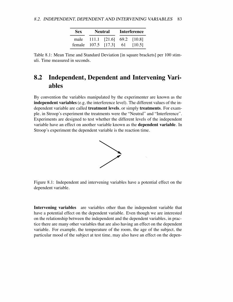
8.2. INDEPENDENT, DEPENDENT AND INTERVENING VARIABLES 83

Sex Neutral Interferencemale 111.1 [21.6] 69.2 [10.8]

female 107.5 [17.3] 61 [10.5]

Table 8.1: Mean Time and Standard Deviation [in square brackets] per 100 stim-uli. Time measured in seconds.

8.2 Independent, Dependent and Intervening Vari-ables

By convention the variables manipulated by the experimenter are known as theindependent variables (e.g, the interference level). The different values of the in-dependent variable are called treatment levels, or simply treatments. For exam-ple, in Stroop’s experiment the treatments were the “Neutral” and “Interference”.Experiments are designed to test whether the different levels of the independentvariable have an effect on another variable known as the dependent variable. InStroop’s experiment the dependent variable is the reaction time.

Figure 8.1: Independent and intervening variables have a potential effect on thedependent variable.

Intervening variables are variables other than the independent variable thathave a potential effect on the dependent variable. Even though we are interestedon the relationship between the independent and the dependent variables, in prac-tice there are many other variables that are also having an effect on the dependentvariable. For example, the temperature of the room, the age of the subject, theparticular mood of the subject at test time, may also have an effect on the depen-


dent variable. Some experimenters emphasize the fact that they are not interestedin the effects of some intervening variables, by calling them nuisance variables.

Good experimental designs control for all possible intervening variables sothat the only systematic source of variation that can explain the results is the in-dependent variable. If a study is poorly designed and intervening variables mayactually explain our results we say that the design lacks internal validity, or thatit has confounding variables. For example, if we choose all the subjects in theneutral condition to be males and all the subjects in the interference condition tobe females, we would say that sex is a confounding variable. The design lacksinternal validity and we would not be able to tell whether the effects on the depen-dent variable are due to the variable “sex” or to the treatment conditions (Neutralvs. Interference).

The art of experimental design consists of making sure intervening variablesdistribute in a “fair” fashion amongst the different treatment conditions so thatthe only systematic differences between the different treatment groups can be at-tributed to the independent variable. The concept of “fair” distribution of theintervening variables is very tricky and we should return to it later. For nowwe’ll just use the concept intuitively and say that when an intervening variableis distributed in a “fair” fashion amongst the treatment conditions we say that thevariable has been controlled. If an intervening variable has been controlled thenit cannot be used to explain away our results. For example, if all our subjects arefemales, and we still find a difference between the two neutral and the interferenceconditions, clearly sex cannot explain this difference. By holding the sex of allsubjects constant we have controlled its possible effect. In scientific parlance we’dsay that sex is a controlled variable. Only when all possible intervening variablesare controlled we can proceed to analyze whether the independent variable X hasan effect on the dependent variable Y . In the next section we discuss the mostcommon methods of control available to scientists.

8.3 Control Methods1. Holding constant: The idea is simple. We make sure an intervening vari-

able is held constant in all our observations. This disqualifies it as a po-tential explanation of our results. For example if all subjects were treatedin the same room at the same temperature, it follows that temperature can-not explain the obtained differences between treatment conditions. Holdingconstant is a rather dramatic method of control but it has its problems. For

8.3. CONTROL METHODS 85

example, if we decide to hold “sex” constant by studying only male sub-jects, we no longer know whether the results are also applicable to femalesubjects. In the lingo of experimental design, we say that holding thingsconstant reduces the external validity of the experiment. External validitysimply means the power to generalize our results to populations larger thanthe specific set of observations obtained in the experiment (e.g., our abilityto say that the Stroop effect occurs to subjects other than the 20 subjectsinvestigated in our experiment).

2. Blocking: The idea in blocking methods is to basically replicate the studywith different levels of the blocked intervening variable. For example wemay “block” age by categorizing subjects into less than 15, 15-30, 30-40,40-50, 50-60, more than 60). Then we can systematically study the exper-imental results within each of the different blocks. An important form ofblocking is blocking by subject, which indicates that we actually block thevariable “subject identity”, thus controlling all intervening variables, knownand unknown, that make subjects different from each other. When we blockby subject, each subject is considered as a block and he/she goes through allthe treatment conditions in the experiment. The idea is to study the effectof a treatment within each subject (e.g. study the difference between theneutral and interference conditions on a subject by subject basis). In thiscase the experiment is said to be within subjects, or repeated measures asopposed to between subjects. Within subject designs are a bit trickier toanalyze and thus we will later dedicate them a special chapter. For now wewill concentrate on between subject designs.

3. Probabilistic Control: This is by far the most important methods of controland it is arguably the one form of control that made rigorous experimentsin the social and biological sciences possible. The fact is that even thoughwe may try to control for known intervening variables, there will always beintervening variables unknown to us that may have a potential effect on ourresults. Hey, may be the position of Jupiter at the time of the experimenthas an effect on some people’s capacity to complete the Stroop task. Whoknows?

So here is the problem: How can we possibly control for intervening vari-ables we cannot even think of? Scientists have found a very ingenious wayto solve this problem. The trick is to give up equal distribution of inter-vening variable in specific experiments, instead what we maintain equal


amongst the treatment conditions is the probability distribution of the vari-able. We think of an ensemble of replications of the same experiment andguarantee that over this entire ensemble, the intervening variables will bedistributed evenly across the different treatment conditions. When we dothat, we say that the intervening variables have been randomized.

We have actually seen control by randomization in previous methods eventhough I avoided calling it by its name. For example, in control by match-ing we first clustered subjects in attempt to distribute intervening variableequally. But since we had differences between the subjects within eachcluster, we then randomly assigned subjects to each treatment condition.In completely randomized designs we simply assign subjects randomly toeach condition without any previous matching.

We can think of the subject identity as an intervening variable that includesall the peculiarities, known and unknown to us, that make each subject dif-ferent from everybody else at test time. We then randomize the effects ofall these known and unknown variables by assigning each subject randomlyacross the different experimental conditions. For example, we could put asmany cards in a hat as the number of different treatment conditions. Thenwe can ask each subject in our experiment to draw a card identifying his/hertreatment condition. Note that by using probabilistic control, experimentsbecome a game of chance, thus the importance of probability theory andstatistics in the analysis of experiments.

Note again that randomization does not guarantee equal distribution of in-tervening variables in single experiments, however it guarantees that on av-erage, if we were to repeat the same experiment many many times, the inter-vening variables will be equally distributed among the different treatmentgroups. Technically speaking, when a variable is randomized, we say that itis a random variable, a mathematical object studied in probability theoryand statistics. We will finish up this chapter with some useful concepts.

4. Matching: You can think of matching as controlled randomization. Forexample, if we simply randomly assign subjects to different treatment con-ditions, it is always possible that in specific experiments exceptional sub-jects accumulate disproportionally in some treatment conditions. Matchingtechniques try to control for these possible imbalances in the following way.First we cluster cluster our subjects in terms of their similarity with respectto a particular variable. Each cluster must has as many subjects as treatment

8.4. USEFUL CONCEPTS 87

conditions. For example, if we wanted to “match by age” in the Stroopexperiment, we would put together groups of 2 people of similar age. Ifwe had 4 subjects with ages 18, 49, 30, and 16, we would make a clusterwith the younger subjects (18, 16) and another cluster with the older sub-jects (49,30). Once the clusters are formed, subjects within each cluster arerandomly assigned to different treatment groups.

5. Statistical Control: In many cases we may not be able to guarantee a uni-form distribution of the intervening variables but we may at least try to makesome aspect of the distribution of variables be the same in all the treatmentgroups. For example, it would be impossible for the room temperature tobe exactly the same all the time but at least we may want to guarantee thanon average the room temperature was the same across treatment conditions.We may also want to make sure that the average age of the subjects is aboutthe same across all treatment groups. Note that equalizing averages does notguarantee equal distributions. For example, treatment group 1 could have50 % 5 year old subjects and 50% 35 year old subjects. Group 2 could havejust 20 year old subjects. Both groups have the same average age but obvi-ously the distribution is completely different. Although this form of controlis rather weak, in some cases it may be all we can do. In such cases wereport in a crystal clear way our method of control and leave it it is up to thescientific community to decide on the validity of our results.

8.4 Useful Concepts1. Experiments vs. Observational studies:

Scientific studies are commonly classified into observational and experi-mental depending on whether the independent variable is observational orexperimental. An independent variable is Experimental if its value is as-signed by the experimenter to the subjects.1 For example if experimentersassign different subjects different dosages of a drug then the drug’s dose isan experimental variable. The crucial point here is that the experimenter,not the subjects, decides which treatment each subject will receive.

1Note that being “experimental” is a property of the independent variable, not a property of thedependent variable. If you want to know whether a study is experimental you need to focus on theindependent variable; do not worry about the dependent variable.


If an independent variable is not experimental then it is called observa-tional. For example, age does not qualify as an experimental variable sinceage cannot be assigned to subjects. All experimenters can do is to classifysubjects according to their age.

The goal of experimental independent variables is to study cause and effectrelationships (e.g., to establish whether a drug is or is not a beneficial to treata particular sickness). Observational variables on the other hand can onlybe used to study relationships, without establishing causes and effects. Forexample, early observational studies about the relationship between smok-ing and cancer showed that smokers tended to have a higher cancer rate thannon-smokers. The dependent variable was whether the subject had cancer.The independent variable was whether the person smoked. Note in this casethe independent variable is observational, since it would be unethical for ex-perimenters to force a group of subject to smoke. The experimenters couldonly classify subjects into smokers or non-smokers. Unfortunately, the re-sults of observational studies like this were inconclusive since they could bedue to an intervening variable that is systematically different between thetwo groups. For example highly stressed subjects could have a propensityto smoke and a higher cancer risk. According to this view, stress, and notsmoking per se, could cause cancer. It could also be the case that subjectswith cancer have a higher propensity to smoke just because cancer stressesyou out. According to this view it is cancer that causes smoking!

A classic example of observational studies involves the analysis of differ-ences between men and women on some dependent variable of interest.Note that since these these studies are observational. We can investigatewhether men and women are different on some dependent variable (e.g.,memory, IQ, or income) but we cannot assess what the causes are for theobtained differences. These causes could be due to trivial variables, such asthe fact that on average men tend to be heavier, or they could be due to com-plex socio-political variables (e.g., the underlying cause for the observeddifferences could be that the educational system treats men and women dif-ferently causing).

2. Exploratory vs. Confirmatory Studies: The distinction between thesetwo different types of research is somewhat subtle, yet important. Confir-matory studies tend to have only a small and well defined set of treatmentsand behaviors under study. Clear a-priori hypotheses are made about what

8.5. EXERCISES 89

to expect in the data and only those a-priori hypothesis are tested. For ex-ample, a confirmatory study may investigate whether taking an aspirin a dayreduces the chances of heart attack. In exploratory studies the experimentersmay have a general idea about what to expect in the data but they are willingto analyze the data in a very wide variety of ways with the hope of findingpotentially interesting results. Exploratory studies are extremely importantin science and they are the source in many cases of new unexpected results.However, the results in exploratory studies tend to be inconclusive basicallybecause by analyzing the data in many different ways it is always possibleto find some sort of pattern that may just be due to chance. You can seethis effect in sports analysis when all sorts of different statistics are usedto explain after the fact why a team has lost or won. In general, resultsof exploratory analysis are treated with caution and attempts are made toreplicate these results with well defined confirmatory experiments.

3. Random Assignment vs. Random Selection: This is a very importantdistinction that novices sometimes confuse. Random selection refers tothe process of selecting a sample from a population of subjects. In manyexperiments this selection does not need to be random. For example, inpsychophysical experiments may times the experimenter himself and hiscolleagues are the subjects of the study, and thus they are not “randomlyselected”. However these non-randomly selected subjects may still be ran-domly assigned to the different treatment conditions. Random selection hasan effect on the external validity of the experiment, our power to generalizeto a larger population. Random assignment has an effect on the internal va-lidity of the experiment, our power to infer that the independent variable isthe one causing the observed results.

8.5 Exercises1. The following questions refer to the experiment outlined at the beginning of

this chapter:

(a) What are the independent and dependent variables?(b) Find intervening variables that where held constant, matched and ran-

domized.(c) Is the experiment experimental or observational? Explain why.


(d) Is the experiment within subjects or within subjects?

2. Design a between subject experiment to test whether bees can distinguishred from green.

3. Design a between subject experiment to test whether human newborns cantell the difference between male and female faces.

4. Design an experiment to test whether caffeine has an effect on the subjectivefeeling of Nervousness. Make sure you specify the following:

(a) Independent variable and its implementation in the different treatmentgroups.

(b) Dependent variable and how you are going to measure it.(c) Intervening variables and how you will control them.

5. Consider the following hypothetical experiment inspired on research byBaker and Theologus [?] on the effects of caffeine on visual monitoring.The purpose of the was to asses the effect of caffeine on a visual monitor-ing task that simulated automobile night driving. Subjects sat in a semi-darkened room approximately 12 oft from a visual display that consisted oftwo 1-inch red lights spaced 6 in. apart. At random intervals ranging from1.5 to 3.5 min., the red lights were driven apart at a rate of 12.56 in/minfor 30 seconds. The geometry of the viewing condition corresponded to adriving situation in which one vehicle followed 60 yd. behind a lead ve-hicle at night driving. The speed at which the lights separated simulatedwhat would be perceived if the lead vehicle reduced its velocity by 0.92mph. Subjects had to continuously monitor the two red-lights and press abutton whenever they detected any separation of the two lights. The reac-tion time, from the beginning of the light separation to the initiation of thesubject;s response was automatically recorded. Testing was conducted overa 4-hr period with 20 trials being administered each hour. for a total of 80responses per subject. During the 4 hour testing period an FM radio tunedto a local station was played to avoid excessive sensory deprivation. Therewere 10 paid male volunteers drawn from universities in the WashingtonDC area. Average age was 29.91 yrs. Subjects were matched by age (e.g.divided into 5 couples with no more than a year difference). Each memberof the age-matched couple was randomly assigned to a different treatment

8.5. EXERCISES 91

group. There were two such treatment groups: 1) A control group of sub-jects given placebo tablets just before testing began and 2 hours before theend of testing. 2) An experimental group of subjects that were given a tabletwith 200 mg. of caffeine just before testing began, and another tablet with200 mg. of caffeine 2 hours before the end of testing. Drug and placebotablet administration was conducted according to a double-blind paradigm,with tablets placed in coded envelopes in a manner unknown to the subjectsand test administrators.

(a) What are the independent and dependent variables?(b) Find intervening variables that where held constant, matched and ran-

domized.(c) Is the study experimental or observational? Explain why.(d) Is the study within subjects or within subjects?

6. What is the difference between external and internal validity?

7. A friend of yours observes that swimmers nicer bodies than other athletes.She concludes that swimming helps have a good body. What’s wrong withthis conclusion? Design an experiment to test your friend’s hypothesis.

8. Read the Abstract, Introduction and Methods sections of the article in Ref-erence [?]. Describe the control methods used in the study.


Chapter 9

Experiments with 2 groups

In this chapter we learn how to apply the T test to experiments with 2 groups. Forexample one group may receive a drug and another group may receive a placebo.The form of the test depends on whether the experiment is performed with dif-ferent subjects in each group or whether the same subjects are used for the twogroups. The first type of experiment is called between subjects or randomized.The second is called within subjects or repeated measures.

9.1 Between Subjects Experiments

In this case we have two sets of random variables. The first set describes measure-ments in a group of subjects, the second set describes measurements in a differentgroup of subjects. The number of subjects per group is the same, and we willrepresent it with the letter n. Thus, the total number of subjects in the experi-ment is 2n. Let X1,1, . . . , X1,n represent the measurements for the first group andX2,1, . . . , X2,n represent the measurements for the second group. Let X1 repre-sent the average of the observations in the first group and X2 the average of the

93

94 CHAPTER 9. EXPERIMENTS WITH 2 GROUPS

observations in group 2. We thus have

X1 =1

n

n∑

i=1

X1,i (9.1)

X2 =1

n

n∑

i=1

X2,i (9.2)

S21 =

1

n & 1

n∑

i=1

(X1,i & X1)2 (9.3)

S2X1

=1

nS2

1 (9.4)

S22 =

1

n & 1

n∑

i=1

(X2,i & X2)2 (9.5)

S2X2

=1

nS2

2 (9.6)

The null hypothesis specifies the expected value of the difference between thesample means of the two groups, i.e, E(X2 & X1 | Hn true). In most experimentsthe null hypothesis says, that this expected value is zero, i.e., that on average thetwo groups are no different. The variable of interest in this case is X2 & X1.We assume that the random variables X1,1, . . . , X1,n and the random variablesX2,1, . . . , X2,n are independent and Gaussian. Moreover we assume that withineach group all the random variables have the same expected value

E(X1,1) = E(X1,2) = · · · = E(X1,n) (9.7)E(X2,1) = E(Y2,2) = · · · = E(Y2,n) (9.8)

(9.9)

and that all the random variables have the same variance

Var(X1,1) = · · · = Var(X1,n) = Var(X2,1) = · · · = Var(X2,n) = $2X (9.10)

where we do not the value of $2X . Note in single group experiments the variable of

interest is the sample mean for that group and we use an estimate of the standarddeviation of the sample mean. In two group experiments the random variable ofinterest is X2 & X1, i.e, the difference between two group means, and thus weneed to come up with an estimate of the standard deviation of (X2 & X1). Note

9.1. BETWEEN SUBJECTS EXPERIMENTS 95

that since X1 and X2 are independent ravs

Var(X2 & X1) = Var(X2) + Var(&X1) = Var(X2) + Var(X1) (9.11)

= 2Var(X1) =2

nVar(X1,1) (9.12)

The last two steps are valid because we assume Var(X1,1) = · · · = Var(X2,n).Thus Var(X1) = Var(X2). We can get an umbiased estimate of the variance ofthe observations by averaging S2

1 and S22 . We represent this pooled estimate as S2

S2 =1

2(S2

1 + S22) (9.13)

An unbiased estimate of the variance of the difference between sample means isas follows

S2X1#X2

=2

nS2 = S2

X2+ S2

X1(9.14)

and the T random variable is defined as follows

T =X2 & X1 & E(X2 & X1 | Hntrue)

SX2#X1

=X2 & X1 & E(X2 & X1 | Hntrue)√

S2X2

+ S2X1

(9.15)In this case the number of degrees of freedom is 2(n & 1) since SX2#X1

is basedon 2(n & 1) independent observations, i.e., n & 1 independent observations in S 2

1

and n & 1 independent observations in S22 .

If Hn is true and the assumptions are met, then T follows the distributiondescribed by Gosset, which is available in tables. The procedure to do one tailedand two tailed tests is identical as for one group experiments provided the newformulas for T and for df are used.

Example A group of 6 migrane patients was gathered and randomly assignedto one of two conditions. In the experimental group subject were given 500 mg ofa new migrane drug whenever they had a migrane access. In the control groupsubjects were given two aspirins. One hour after the access, subjects were askedto rank from 0 to 100 how bad the headache was. 0 meaning, “headache? whatheadache?”, and 100 meaning “I cant take it anymore”. The results were asfollowsExperimental Group =[10, 30, 20]Control Group = [56, 64, 60]


First of all we compute the values taken by the relevant random variables in ourexperiment

X1 = (10 + 30 + 20)/3 = 20 (9.16)X2 = (56 + 64 + 60)/3 = 60 (9.17)

S21 = ((10 & 20)2 + (30 & 20)2 + (20 & 20)2)/2 = 100 (9.18)

S22 = ((56 & 60)2 + (64 & 60)2 + (60 & 60)2)/2 = 16 (9.19)

SX1#X2=

√100/3 + 16/3 = 6.21 (9.20)

In our case it makes sense to use a one tailed test, since we are trying to reject thehypothesis that the aspirin works better or equal to the new drug. Thus the nullhypothesis tells us that E(X2 & X1 | Hn true) * 0. The extreme case, i.e., whatwe call Hx says E(X1 & X2 | Hx true) = 0. Thus,

T =X2 & X1 & E(X2 & X1 | Hx true)

SX2#X1

=(60 & 40) & 0

6.21= 3.22 (9.21)

The number of degrees of freedom is (2)(3&1) = 4. We go to tables and find thatfor 4 degrees of freedom P (T > 2.13 |Hx true) = 0.05. Thus the critical value is2.13. Since the value taken by T is larger than 2.13 we have enough evidence toreject the null hypothesis. We can say that the new drug works better than aspirin.

9.1.1 Within Subjects ExperimentsIn the previous experiments we assumed all the measurements were independent.In within subjects experiments this assumption is clearly incorrect: if we test thesame subjects in the two groups, then the random variables in the first group willbe related to the random variables in the second group. This type of experimentsare called “repeated measurements” or within subjects. In this case we work withthe differences between the observations obtained in the two groups on a subjectby subject basis

Dj = X2,j & X1,j (9.22)

and the sample average of the difference would be

D =1

n

n∑

j=1

Dj = X2 & X1 (9.23)

9.1. BETWEEN SUBJECTS EXPERIMENTS 97

In most cases the null hypothesis says that there is no differences in the expectedvalues of the two groups, i.e., E(D |Hn true) = 0. The T random variable follows

T =D & E(D | Hn true)

SD

(9.24)

This effectively transforms a 2 group experiment into a single group experimentthat can be analyzed with the techniques we saw in the previous chapter.

Example Three undergraduate students from UCSD volunteered to participateon an experiment to test the effect of caffeine on reaction time. Each studentwas tested in two different conditions with the tests being separated in time byone week. In one condition the subjects drunk a double espresso. In the otherconditions the subjects drunk a double decaffeinated espresso. The order of thetwo conditions was randomly assigned. On each condition, the subjects weretested 15 minutes after drinking the espresso. Subjects were tested on a task thatrequired rapid reaction to a stimulus. The average reaction time in millisecondsof each subject was recorded. The results were as followsCaffeine Condition =[10, 30, 20]Decaf Condition = [56, 64, 60]The first number on each condition corresponds to the first subject, second num-ber to second subject and third number to the third subject. Is the difference inreaction time between the two conditions statistically significant?

This is a repeated measures experiment so the T-test would be based on thedifference measurements obtained for each of the three subjects.

D1 = 10 & 56 = &46 (9.25)D2 = 30 & 64 = &34 (9.26)D3 = 20 & 60 = &40 (9.27)

D = (&46 & 34 & 40)/3 = &40 (9.28)

S2D =

1

2((62) + (62) + 02) = 18 (9.29)

S2D = 18/3 = 6 (9.30)

T =18 & 0'

6= 7.35 (9.31)

df = (3 & 1)8 = 2 (9.32)P (T | Hx > 2.91 True) = 1/20 Obtained using T-tables (9.33)


Thus the critical value is 2.91. Since 7.35 is larger than 2.91. The difference inreaction time between the two groups is statistically significant.

9.2 Exercises1. A San Diego based biotek company is testing whether a new drug has a good

effect on amnesia, the inability to remember recently presented materials.The sample consisted of 8 amnesic patients that volunteered to participatein the experiment. The subjects were randomly assigned to either the exper-imental group (drug) or the control group (placebo). Subjects were treatedwith 125 mg a day of the drug or the placebo for 30 days. After one monthsubjects were given a list of 100 training pictures one at a time at 2 secondintervals. Half an hour later subjects were presented 200 new pictures: the100 training pictures plus 100 new ones. Subjects were asked to discrim-inate whether the pictures were old or new. The dependent variable wasthe percentage of correctly discriminated pictures. The results in the exper-imental group were as follows:{61, 60, 59, 60}. The results in the controlgroup were as follows: {50, 51, 50, 49}.

(a) Is the experiment randomized or within subjects?(b) Specify the null hypothesis if you were to use a two tailed test.(c) Do you have enough evidence to reject this null hypothesis?(d) Specify the null hypothesis if you were to use a one tailed test.(e) Do you have enough evidence to reject this null hypothesis?(f) What assumptions did you make?(g) A replication of the same experiment with a different random sample

of subjects results in a control group mean of 10 instead of 50? Doyou find this surprising? Justify your response.

(h) Repeat the analysis assuming the same subjects are used in both groups.For example, Subject 1 gets a score of 61 when he/she takes a drug anda score of 50 when he/she takes the placebo.

Chapter 10

Factorial Experiments

NOTE FROM JAVIER R. Movellan: This chapter may be particularly buggy. Useat your own risk.

10.1 Experiments with more than 2 groupsIn this chapter we will apply the T-test to experiments that involve more than twotreatment groups. The basic ideas are the same as in single group and two groupexperiments. The only difference is that we use information from all the groupsto get better estimates of the variance. The experimental design we will address iscalled “between subjects” indicating that each of the treatment groups is made ofdifferent randomly assigned subjects.

Suppose we want to study the joint effects of caffeine and alcohol on the time ittakes people to respond to a red light. Eight volunteer students from the CognitiveScience Department at UCSD were randomly assigned to one of four treatmentgroups: Group 1) Each subject in this group has a non-alcoholic beer and a decaf-feinated coffee. Group 2) Each subject in this group has an alcoholic beer and adecaffeinated coffee. Group 3) Each subject in this group has a non-alcoholic beerand a regular coffee. Group 4) Each subject in this group has an alcoholic beerand a regular coffee. Each of the 8 subjects in our sample was measured in termsof the times it took them to do a test that involved pushing a pedal in response toa red light. Table 11 shows the results of the experiment

Suppose we want to know whether alcohol has an effect on people that takeregular coffee. In this cases the null hypothesis would be that the alcohol has noeffect, i.e.,

99

100 CHAPTER 10. FACTORIAL EXPERIMENTS

E(X4 & X3 | Hn true) = 0 (10.1)

where Xi represents the sample mean of group i in the experiment. We could testthis hypothesis restricting our analysis to groups 3 and 4. This would simply be atwo group experiment that we already know how to analyze. However there is abetter way to do things. The idea is to use a pooled estimate of the variance basedon the 4 groups, instead of just two groups. The advantage of such an estimate isthat it is based on more observations. If our experiment has a different groups, thepooled estimate would be

S2 =1

a(S2

1 + S22 + S2

3 + · · ·+ S2a) (10.2)

and it would have (a)(n & 1) degrees of freedom. We know

Var(X4 & X3) = 2Var(X1) =2

nVar(X1,1) (10.3)

thus our estimate of this variance will be

S2X4#X3

=2

nS2 (10.4)

and the T random variable would be

T =X4 & X3√(2/n)S2

(10.5)

Table 10.1:NoAlcohol Alcohol

NoCaffeine 3 1 7 5Caffeine 1 1 10 16

10.2. INTERACTION EFFECTS 101

In our example

X1 = 2 (10.6)X2 = 6 (10.7)X3 = 1 (10.8)X4 = 13 (10.9)

S21 =

1

2 & 1((3 & 1)2 + (1 & 1)2) = 2 (10.10)

S22 =

1

2 & 1((7 & 6)2 + (5 & 6)2) = 2 (10.11)

S23 =

1

2 & 1((1 & 1)2 + (1 & 1)2) = 0 (10.12)

S24 =

1

2 & 1((10 & 13)2 + (13 & 16)2) = 18 (10.13)

S2 =1

4(2 + 2 + 0 + 18) =

11

2(10.14)

T =13 & 1 & 0√

22

112

= 5.11 (10.15)

df = 4; (10.16)

we see in tables thatP (T > 2.77 | Hn true) = 1/20 (10.17)

10.2 Interaction EffectsIn many cases it is important to know whether the effect of a treatment changeswhen administered in combination with other treatments. For example in manycases we need to know whether a drug has the same effect when combined withother drugs. This concept is so important that statisticians gave it a special name:“interaction effects”. In general, if the effect of a treatment changes when com-bined with other treatments, we say that the treatments interact, or that the ef-fects are non-additive. Otherwise we say that the treatments are additive, orthat there is no interactions.

The simplest experimental design that allows to study whether treatments in-teract consists of 4 groups formed by the combination of two treatments of one

102 CHAPTER 10. FACTORIAL EXPERIMENTS

factor (e.g., caffeine versus no caffeine) and two treatments of another factor (e.g.,alcohol versus no alcohol). This type of design is called a 2 . 2 factorial design.

Now we need to translate the concept of interaction into a specific testablehypothesis. Let’s take the example experiment we have analyzed so far. If thereis no interaction between alcohol and caffeine, then the effect of alcohol shouldbe the same regardless of whether a person takes regular or decaffeinated coffee.We measure the effect of alcohol when combined with decaffeinated coffee asE(X2 & X1) and the effect of alcohol when combined with regular coffee asE(X4 & X3). Thus, if there is no interactions, these two effects have to be thesame. In other words, The null hypothesis of no interaction effects says that

E[(X2 & X1) & (X4 & X3) | Hn true] = 0 (10.18)

or equivalentlyE[X2 + X3 & X1 & X4 | Hn true] = 0 (10.19)

So the random variable of interest is X2 + X3 & X1 & X4. Since we know that

Var(X2 + X3 & X1 & X4) = 4Var(X1) =4

nVar(X1,1) (10.20)

then our estimate of the standard deviation of X2 + X3) & X1 & X4 is

S2X2+X3#X1#X4

=4

nS2 (10.21)

and it has (a)(n & 1) degrees of freedom. The T random variable follows

T =X2 + X3 & X1 & X4 & E(X1 & X4 | Hn true)

SX2#X3#X1#X4

(10.22)

In our example,

T =6 + 1 & 2 & 13√

(4/2)(11/2)= 2.41 (10.23)

2df = (4)(2 & 1) = 4 (10.24)

For 4 df the critical value is 2.71 and thus we do not have enough evidence toreject the null hypothesis. We cannot say that alcohol and caffeine interact.

Chapter 11

Confidence Intervals

NOTE FROM JAVIER: This chapter has not been properly debugged. Use at yourown risk.

In this chapter we study a method to bracket expected values based on sampleinformation. We may want to bracket expected values of the mean of a group, or the difference between sample means of two groups, or the difference of thedifference between sample means of 4 groups (we’d do so to analyze interactions).In all cases the basic ideas are the same. While hypothesis testing and intervalestimation are closely related, the later method is in general more informative forthe following two reasons: 1) Classical hypothesis testing does not tell us theprobability that our decisions be correct. Classical interval estimation does tell usabout this. 2) Classical interval estimation methods are easier to relate to Bayesianmethods so they provide a better foundation for a way of analyzing experimentsconsistent with classical and Bayesian approaches.

We will see an example of interval estimation using the data from an experi-ment we used in a previous chapter. Here is a re cap of the experiment at hand:

Suppose we want to study the joint effects of caffeine and alcohol on the time ittakes people to respond to a red light. Eight volunteer students from the CognitiveScience Department at UCSD were randomly assigned to one of four treatmentgroups: Group 1) Each subject in this group has a non-alcoholic beer and a de-caffeinated coffee. Group 2) Each subject in this group has an alcoholic beer anda decaffeinated coffee. Group 3) Each subject in this group has a non-alcoholicbeer and a regular coffee. Group 4) Each subject in this group has an alcoholicbeer and a regular coffee. Each of the 8 subjects in our sample was measuredin terms of the times it took them to do a test that involved pushing a pedal inresponse to a red light. Table 11 shows the results of the experiment

103

104 CHAPTER 11. CONFIDENCE INTERVALS

Suppose we are interested in bracketing the value of E(X3). To do so considerthe following T random variable

T =X3 & E(X3)

SX3

(11.1)

Note that now we do not condition on the null hypothesis being true. We simplytreat E(X3) as a fixed, yet unknown number. Thus, since we are using the correctexpected value, T will follow Gosset’s t-distribution. In previous chapters we sawthat for this particular experiment,

X3 = 1 (11.2)S2 = 11/2 (11.3)

df = 4 (11.4)c = 2.77 (11.5)

where c was obtained using T-tables so that P (T ( c) = 1/40. Moreover. sinceX3 is based on two observations

SX3=

√S2/2 =

√(1/2)(11/2) = 1.65 (11.6)

Now notice the following,

P (&c * T * c) = 0.95 (11.7)

= P (&c * X3 & E(X3)

SX3

* c) (11.8)

= P (&cSX3* X3 & E(X3) * cSX3

) (11.9)= P (&X3 & cSX3

* &E(X3) * &X3 + cSX3) (11.10)

= P (X3 + cSX3( E(X3) ( cX3 & cSX3

) (11.11)(11.12)

Table 11.1:NoAlcohol Alcohol

NoCaffeine 3 1 7 5Caffeine 1 1 10 16

105

Now lets define the random variables L and U to represent the upper and lowerlimits of our intervals,

L = X3 & cSX3(11.13)

U = X3 + cSX3(11.14)(11.15)

We have learned thatP (E(X3) ! [L, U ]) = 0.95 (11.16)

In other words, there is a 95 % chance that the random interval [L, U ], will coverthe true value of E(X3). Note that the interval [L, U ] is random, i.e., it changeswith the outcome of the experiment, and E(X3) is not random, i.e., it is a fixedyet unknown number.

Example In our experiment,

L = X3 & cSX3= 1 & (2.77)(1.65) = 3.57 (11.17)

U = X3 & cSX3= 1 + (2.77)(1.65) = 5.57 (11.18)

In our particular experiment, the confidence interval for E(X3), the expectedvalue of the mean of the third group, is [3.57, 5.57] we do not know whetherin this particular experiment the confidence interval brackets the expected value,however we know that in 19/20 experiments, the procedure we used will be cor-rect.

106 CHAPTER 11. CONFIDENCE INTERVALS

Appendix A

Useful Mathematical Facts

1. Symbols

(a) " “Is defined as”(b) n! “n-factorial”

n! =

{1 if n = 0

(1)(2)(3) · · · (n) if n "= 0(A.1)

(c) Sterling’s approximation

n! +'

2"n(n

e)n (A.2)

(d) e = 2.718281828 · · · , the natural number(e) ln(x) = loge(x) The natural logarithm(f) 1A The indicator (or characteristic) function of the set A. It tells us

whether or not an element belongs to a set. It is defined as follows,1A : ! ) {0, 1}.

1A(!) =

{1 for all ! ! A % !

0 for all ! ! Ac % !(A.3)

Another common symbol for the indicator function of the set A is 'A

2. The Greek alphabet

107

108 APPENDIX A. USEFUL MATHEMATICAL FACTS

A % alpha I ( iota P ) rhoB & beta K * kappa $ $ sigma% + gamma & # lambda T , tau" - delta M µ mu ' . upsilonE / epsilon N 0 nu # 1 phiZ 2 zeta ( ' xi X 3 chiH 4 eta O o omicron ) 5 psi* 6 theta + " pi ! ! omega

3. Series

1 + 2 + 3 + · · ·+ n =(n)(n + 1)

2(A.4)

a0 + a1 + a2 + · · · + an#1 =1 & an

1 & a(A.5)

1 + a + a2 + · · · =1

1 & a, for|a| < 1 (A.6)

a + 2a2 + 3a3 + · · · =a

(1 & a)2, for0 < a < 1 (A.7)

ex ="∑

n=0

xn

n!(A.8)

cos(x) = 1 & x2

2!+

x4

4!& x6

6!+ · · · (A.9)

sin(x) = x & x3

3!+

x5

5!& x7

7!+ · · · (A.10)

ejx = cos(x) + j sin(x) where j"'&1 (A.11)

109

4. Binomial Theorem

(a + b)n =n∑

m=0

(n

m

)an#m bm (A.12)

where (n

m

)" n!

(m!) (n & m)!(A.13)

Note from the binomial theorem it follows that

2n =

(n

0

)+

(n

1

)+ · · ·+

(n

n

)(A.14)

5. Exponentials

a0 = 1 (A.15)

am+n = am an (A.16)

a#n =1

an(A.17)

(ab)n = anbn (A.18)

6. Logarithms

a(loga(x)) = x (A.19)

loga(x y) = loga(x) + loga(y) (A.20)

loga(xy) = y loga(x) (A.21)

loga(1) = 0 (A.22)


loga(a) = 1 (A.23)

loga(x) = (logb(x))/ logb(a) (A.24)

7. Quadratic formulaThe roots of the equation ax2 + bx + c = 0 are

x =&b ±

'b2 & 4ac

2a(A.25)

8. Factorizations

a2 & b2 = (a & b)(a + b) (A.26)

9. Trigonometry

tan(%) =sin(%)

cos(%)(A.27)

sin2(%) + cos2(%) = 1 (A.28)

sin(% + &) = sin(%) cos(&) + cos(%) sin(&) (A.29)

cos(% + &) = cos(%) cos(&) & sin(%) sin(&) (A.30)

tan(% + &) =tan(x) + tan(y)

1 + tan(x) tan(y)(A.31)

10. Hyperbolics

sinh(x) =ex & e#x

2(A.32)

cosh(x) =ex + e#x

2(A.33)

111

tanh(x) =sinh(x)

cosh(x)(A.34)

11. Complex NumbersWe use the convention j"

'&1. There are three ways to represent a com-

plex number

(a) Cartesian representation

x = (xr, xi) = xr + jxi (A.35)

where xr and xi are the real and imaginary components of x.

(b) Polar representation:

|x|"√

x2r + x2

i (A.36)

is called the magnitude of x.

∠x"arc tanxi

xr(A.37)

is called the phase of x.

(c) Exponential representation

x = |x|ej∠x = |x|(cos(∠x), sin(∠x)) (A.38)

Operation on complex numbers:

(a) Addition/Substraction:

(xr, xi) + (yr, yi) = (xr + yr, xi + yi) (A.39)

(b) Multiplication

|(xy)| = |x||y| (A.40)

∠(xy) = ∠x + ∠y (A.41)


(c) ConjugationThe complex conjuage of x = (xr, xi) is x = (xr,&xi). Note |x| =|x| and ∠(x) = &∠(x).

(d) Inner ProductLet x = (x1, · · · , xn) and y = (y1, . . . , yn) be complex vectors (i.e.,each component of x and of y is a complex number). The inner prouctof x and y is defined as follows

< x, y >= x · y =n∑

i=1

xiyi (A.42)

12. DerivativesLet y = f(x)

dy

dx= lim

!x!0(f(x + "x) & f(x))/"x (A.43)

Here are some alternative representations of the derivative

f $(x) = y$ =dy

dx=

d

dxy =

df(x)

dx=

d

dxf(x) =

df(u)

du|u=x (A.44)

• Exponential:d

dxexp(x) = exp(x) (A.45)

• Polynomial:d

dxxm = mxm#1 (A.46)

• Logarithmd

dxln x =

1

x(A.47)

• Sined

dxsin x = cos x (A.48)

• Cosine

d

dxcos x = & sinx (A.49)

113

• Linear combinations

d

dx((a)f(x) + (b)g(x)) = (a)

d

dxf(x) + (b)

d

dxg(x) (A.50)

• Productsdf(x)g(x)

dx= f(x)

dg(x)

dx+ g(x)

df(x)

dx(A.51)

• Chain RuleLet y = f(x) and z = g(y)

dy

dx=

dz

dy

dy

dx(A.52)

You can think of the chain rule in the following way: x changes ywhich changes z. How much z changes when x changes is the productof how much y changes when x changes times how much z changeswhen y changes. Here is a simple example that uses the chain rule

d exp(ax)

dx=

d exp(ax)

dax

ax

dx= exp(ax)(a) (A.53)

13. Indefinite IntegralsThe indefinite integral of the function f is a function whose derivative isf (i.e., the antiderivative of is f ). This function is unique up to addition ofarbitrary constant. The expression

∫f(x)dx = F (x) + C (A.54)

means that F $(x) = f(x). The C reminds us that the derivative of F (x)plus any arbitrary constant is also f(x).

• Linear Combinations∫

af(x) + bg(x)dx = a

∫f(x)dx + b

∫g(x)dx (A.55)

• Polynomials∫

xmdx =xm+1

m + 1+ C (A.56)


• Exponentials∫

exp(x)dx = exp(x) + C (A.57)

• Logarithms∫

1

xdx = ln(x) + C (A.58)

• Integration by parts∫

f(x)g$(x)dx = f(x)g(x) &∫

f $(x)g(x)dx (A.59)

The formula for integration by parts easily follows from the formulafor the derivative of the product of f(x)g(x).

History• The first version of this document was written by Javier R. Movellan in

1994. The document was 6 pages long.

• The document was made open source under the GNU Free DocumentationLicense Version 1.1 on August 9 2002, as part of the Kolmogorov project.

Appendix B

Set Theory

Intuitively we think of sets as collections of elements. The crucial part of thisintuitive concept is that we are willing to treat sets as entities distinguishable fromtheir elements. Sometimes we identify sets by enumeration of their elements. Forexample, we may talk about the set whose elements are the numbers 1, 2 and 3.In mathematics such sets are commonly represented by embracing the elementsof the set using curly brackets. For example, the set {1, 2, 3} is the set whoseelements are the numbers 1, 2 and 3. Sometimes sets are defined using someproperty that identifies their elements. In such case it is customary to representthe sets using the following formula

{x : x has a particular property} (B.1)

For example, the set {1, 2, 3} can be represented as

{x : x is a natural number smaller than 4}. (B.2)

The intuitive concept of sets as collections of elements is useful but it can onlytake us so far. You may complain that we have not really defined what a set issince we have not defined collections and we have not specified what qualifies asan element. We have not specified either what qualifies as a property. Considerfor example the proposition {x : x is not an element of x}, i.e., the set of setswhich are not elements of themselves. We can prove by contradiction that sucha set does not exist. Let’s assume that this set exists and lets represent it withthe symbol y. If y is an element of y then, since all the elements of y are not anelement of themselves it follows that y is not an element of y. Moreover, if y isnot an element of y then, y must be an element of y. In other words, if we assume

115

116 APPENDIX B. SET THEORY

the set y exists we get a contradiction. Therefore we have to conclude that y doesnot exist. Using similar reasoning one can also show that the set of all sets doesnot exist either (see proof later in this document). But this raises deep questions:

1. What does it mean to say that a set exists or does not exist? For exampleLeopold Kronecker, a German mathematician born in 1823, claimed thatthe only numbers that assuredly exist are the natural numbers (1,2,3 ...).According to him the set of real numbers are just a fantasy that does notexist. But think about it, what criteria, other than authority, can we use todecide whether the natural numbers or the real numbers exist?

2. How can we tell whether something is or is not a set?

3. What are valid elements of a set?

Axiomatic set theory was developed to provide answers to such questions. Inaxiomatic set theory:

1. A set exists if the proposition that asserts its existence is logically true.Moreover within this theory there are only sets so if a formal object is not aset, it does not exist.

2. If the assumption that an object exists leads to a contradiction we can assertthat that object does not exist, or equivalently, that it is not a set.

3. There are no atomic elements: An object exists if and only if it is a set. Ofcourse sets can have elements but those elements must be sets themselvesotherwise they would not exist.

One “annoying” aspect of axiomatic set theory is that sets become a logicalabstraction detached from our everyday experience with collections of physicalobjects. You should think of mathematical sets as logical “objects” which are partof a formal structure. Within this theory to say that an object exists is the same assaying that it is a set. To say that an object does not exist is the same as saying thatit is not a set. Everyday collection of physical objects are no longer sets in thistheory and thus they do not exist. While this approach may strike you as peculiar,it turns out to be extremely powerful and in fact it has become the foundationof mathematics. The formal structure of set theory while independent from thephysical world provides very useful tools to model the world itself. The key is todevelop set structures constrained in ways that mirror essential properties of the

117

physical world. For example, the properties of the set of natural numbers (i.e.,1,2,3, . . .) mirrors our experience counting collections of physical objects.

Axiomatic set theory is a first order logical structure. First order logic workswith propositions, i.e., logical statements constructed according to the rules oflogic and that can take two values. For convenience we call these two values“True” and “False”. Set theory, and thus the entire body of mathematics reducesto logical propositions that use the following elements:

1. Variables (e.g., a, b, . . . x, y, z) which stand for sets.

2. The predicate !, which stands for element inclusion. For example, if theproposition (x ! y) takes the value true, we know that both x and y are setsand that x is an element of y. For example, the proposition

{1, 2, 3} ! {{1, 2}, {4, 5}, {1, 2, 3}} (B.3)

takes the value “True”.

3. Logical operators

(a) ¬P , where ¬ is the logical “negation” operator.(b) P / P , where / is the logical “and” operator.(c) P 0 P , where 0 is the logical “or” operator.(d) P ) P , where ) is the logical “implication” operator.(e) P1P , where 1 is the logical “bijection” operator.(f) 2xP is the logical “for-all” quantifier.(g) 3xP is the logical “exists” quantifier.

The names of the different operators (i.e., “negation”, “and”, “or”, “implication”...) are selected for convenience. We could have given them completely differentnames, all we really need to know is how they operate on propositions.

All propositions in set theory are built out of atomic propositions of the form(x ! y) connected using the logical operators. If P and Q are propositions, e.g.,P could be (x ! y) and Q could be (y ! z ) then ¬P , P / P , P 0 Q P ) Q,P1Q, 2xP and 3xP are also propositions.

The effect of the connectives on the truth value of propositions is expressedin Table B . Thus, if the proposition P takes value “True” and the proposition Qtakes the value “False” then the proposition (P /Q) takes the value “False”. The


P Q ¬P P / Q P 0 Q P ) Q P1QT T F T T T TT F F F T F FF T T F T T FF F T F F T T

Table B.1: The truth tables of the logical operators. T stands for “True” and F for“False”.

propositions 2xP and 3xP tell us that x is a variable that can take as value anyformal object that qualifies as a set. It also tells us that P is a proposition whosetruth value depends on x. For example, P could be (x ! y) 0 (x ! z), wherey and z are fixed sets and x acts as a variable. The proposition 2xP takes thevalue “True” if P takes the value “True” for all sets. The proposition 3xP takesthe value “True” if there is at least one set for which P takes the value “True”.Remember when we say for all sets we do not mean sets of physical objects. Infact we still have to define what we mean by set.

B.1 Proofs and Logical Truth

Sometimes we treat propositions as formulas whose truth value depends on thetruth values taken by variables in the proposition. For example if P and Q arepropositional variables then the P / Q is a propositional formula whose truthvalue depends on the specific truth values taken by P and Q. We say that a propo-sitional formula is logically true if for all valid combinations of truth values ofthe elements in the formula, the formula can only take the value “True”. Forexample for the formula (P 0 ¬P ) there is only two valid combination of truthvalues for P and ¬P : “True, False” and “False, True”. In both case the formula(P 0 (¬P )) takes the value “True” and thus we say that it is logically true. Sim-ilarly if a propositional formula can only take “False” values we say that it islogically false. For example (P / (¬P )) is logically false. A proof is a processthat shows a propositional formula is logically true.

B.2. THE AXIOMS OF SET THEORY 119

B.2 The Axioms of Set TheoryTo simplify the presentation of axiomatic set theory I will use “pseudocode”, i.e.,a combination of logical propositions, mathematical symbols, and English state-ments. I do so under the understanding that all these statements can be written aspure logical propositions.

I will use the symbol "! in propositions of the form (x "! y) as an alternativenotation to ¬(x ! y). I will use the formula

3{x : P} (B.4)

as an alternative notation to the propositional formula

3y2xP (B.5)

This formula simply says that there is a set of elements that satisfy the propositionP . If the formula takes the value “True” then the symbols {x : P} refers to a setthat make the proposition 2xP “True”. When a set x makes the proposition Ptrue, I will say that x satisfies P . For example the set 1 satisfies the propositionalformula (x ! {1, 2}).

In set theory all existing objects are sets. If an object exists it is a set otherwiseit does not exist. To remind us of the fact that sets include elements we sometimesrefer to sets as a collection of sets, or as a families of sets. This is just a “humanfactors” trick since the theory makes no distinction between sets, families, collec-tions or elements. In axiomatic set theory elements, collections, and families arejust sets.

Axiomatic set theory is commonly presented using 9 redundant axioms, whichare the foundation of all mathematical statements.

B.2.1 Axiom of Existence:An axiom is a restriction in the truth value of a proposition. The axiom of exis-tence forces the proposition

3y2x(x "! y) (B.6)

to take the value “True”. We call call the sets that satisfy 2x(x "! y) empty sets.Thus the axiom of existence tells us that there is at least one empty set, we willsee later that in fact there is only one empty set.


B.2.2 Axiom of Equality:This axiom is also called the axiom of extensionality and it defines the predicate“=”. For mnemonic convenience when the proposition (x = y) takes the value“True” we say that the sets x and y are equal. In order to define how the symbol“=” works it is convenient to create a new predicate, which we will symbolize as#. The new predicate works as follows: For all sets u and v if the proposition

2x(x ! u) ) (x ! v) (B.7)

is true then the proposition (u # v) is true. For mnemonic convenience if theproposition (u # v) takes the value “True” we say that u is a subset of v.

The axiom of equality says that if the proposition (u # v) / (v # u) is truethen the proposition (u = v) is true. In other word, the proposition

2u(u ! x1u ! y) ) (x = y) (B.8)

takes the value “True”. The formula (x "= y) is used as an alternative notation to¬(x = y). We will now use the axiom of equality to prove that there is only oneempty set.

Theorem: The empty set is unique.

Proof: Let x and y be empty sets, then u ! y and u ! x are always false forall sets u. Thus (u ! y1u ! x) is true for all sets u and since by the axiom ofequality

(2u(u ! x1u ! y)) ) (x = y) (B.9)is true then it follows that (x = y) must be true. Hereafter we identify the emptyset with the symbols ! or alternatively with the symbol {}.

!

B.2.3 Axiom of Pair:So far set theory has only given us one set: the empty set. The axiom of pairbrings new sets to life. The axiom of pair says that if x and y exist (i.e., if they aresets) there also exists a set whose only elements are x and y. We will representsuch set as {x, y}. The axiom of pair forces the proposition

2x2y3{x, y} (B.10)


to take the value “True”. The set made out of the sets a and a is symbolized as{a, a} or {a} and is called the singleton whose only element is a. So startingwith the empty set !, it follows that the set {!} exists. Note that ! and {!} aredifferent since the first has no element and the second has one element, which isthe empty set.

Ordered pairs: The ordered pair of the sets x and y is symbolized (x, y) anddefined as follows

(x, y)"{{x}, {x, y}} (B.11)

where " stands for “equal by definition”.

Exercise: Prove that two ordered pairs (a, b) and (c, d) are equal if and only ifa = b and c = d.

Ordered sequences: Let x1, . . . , xn be sets. The ordered sequence (x1, . . . , xn)is recursively defined as follows

(x1, · · · , xn) = ((x1, · · · , xn#1), xn) (B.12)

Exercise: Prove that two n-tuples pairs (a1, . . . , an) and (b1, . . . , bn) are equalif and only if a1 = b1 and a2 = b2 and ... an = bn.

B.2.4 Axiom of Separation:

This axiom tells us how to generate new sets out of elements of an existing set.To do so we just choose elements of an existing set that satisfy a proposition.Consider a proposition P whose truth value depends on the sets u and v, forexample, P could be (u ! v). The axiom of separation forces the proposition

3{x : (x ! u) / P} (B.13)

to take the value “True” for all sets u, v and for all propositions P with truth valuesdependent on u and v.


Fact: There is no set of all sets.The proof works by contradiction. Assume there is a set of all sets, and call it u.Then by the axiom of separation the following set r must exist

r = {x : (x ! u) / (x "! x)} (B.14)

and since (x ! u) is always true, this set equals the set

{x : x "! x} (B.15)

Then (r !)r1(r "! r) which is a logically false proposition. Thus the set of allsets does not exist (i.e., it is not a set).

Intersections: The intersection of all the sets in the set s, or simply the inter-section of s is symbolized as %s and defined as follows:

%s = {x : 2y( (y ! s) ) (x ! y) )} (B.16)

For example, if s = {{1, 2, 3}, {2, 3, 4}} then %s = {2, 3}. The axiom of sepa-ration tells us that if s exists then %s also exists. We can then use the axiom ofequality to prove that %s is in fact unique. For any two sets x and y, we representtheir intersection as x % y and define it as follows

x % y" % {x, y} (B.17)

For example, if x = {1, 2, 3} and y = {2, 3, 4} then

x % y = %{{1, 2, 3}, {2, 3, 4}} = {2, 3} (B.18)

B.2.5 Axiom of Union:It tells us that for any set x we can make a new set whose elements belong toat least one of the elements of x. We call this new set the union of x and werepresent it as $x. For example, if x = {{1, 2}, {2, 3, 4}} then $x = {1, 2, 3, 4}.More formally, the axiom of union forces the proposition

2s3 $ s (B.19)

to be true. Here $s is defined as follows

$s"{x : 3y(y ! s) / (x ! y)} (B.20)


For example, if x = {{1, 2, 3}, {2, 3, 4}} then $x = {1, 2, 3, 4}. Using the axiomof equality $x can be shown to be unique. For any two sets x and y, we define theunion of the two sets as follows For example,

{1, 2, 3} $ {2, 3, 4} = {1, 2, 3, 4} (B.21)

x $ y" $ {x, y} (B.22)

B.2.6 Axiom of Power:This axiom tells us that for any set x the set of all subsets of x exists. We callthis set the power set of x and represent it as P(x). More formally, the axiom ofpower forces the proposition

2s3{x : x # u} (B.23)to take the value “True”. For example, if s = {1, 2} then

P(s) = {{1}, {2}, !, {1, 2}}. (B.24)

Cartesian Products: The Cartesian product of two sets u and v, is symbolizeda . b and defined as follows

a . b = {(x, y) : (x ! a) / (y ! b)} (B.25)

Using the axioms of separation, union and power, we can show that x ! y existsbecause it is a subset of P(P(x $ y)). Using the axiom of identity we can showthat it is unique.

Functions: A function f with domain u and target v is a subset of u . v withthe following property: If (a, c) and (b, c) are elements of f then a = b. Moreformally, if the proposition

2a2b2c(((a, c) ! f) / ((b, c) ! f) ) (a = b)) (B.26)

takes the value “True” then we say that the set f is a function.The following formulae are alternative notations for the same proposition:

(x, y) ! f (B.27)y = f(x) (B.28)x 4) f(x) (B.29)x 4) y (B.30)


B.2.7 Axiom of Infinity:This axiom forces the proposition

3s2x(x ! s) ) ({x, {x}} ! s) (B.31)

to take the value “True”. In English this axiom tells us that there is a set s suchthat if x is an element of s then the pair {x, {x}} is also an element of s. Sets thatsatisfy the proposition

2x(x ! s) ) ({x, {x}} ! s) (B.32)

are called inductive (or infinite) sets.

Natural numbers: The natural numbers plus the number zero are defined as theintersection of all the inductive sets and are constructed as follows:

0 " {} (B.33)1 " {0, {0}} = {{}, {{}}} (B.34)2 " {1, {1}} = {{{}, {{}}}, {{{}, {{}}}}} (B.35)...

The axiom of existence in combination with the axiom of infinity guaranteethat these sets exist. Note that the symbols 1, 2, · · · are just a mnemonic conve-nience. The bottom line is that numbers, and in facts all sets, are just a bunch ofempty curly brackets!

B.2.8 Axiom of Image:Let f : u ) v be a function (i.e, a subset of u. b). Define the image of u under fas the set of elements for which there is an element of u which projects into thatelement. We represent that set as If(u). More formally

If (u) = {y : 3x(x ! u) / (f(x) = y)} (B.36)

The axiom of image, also called the axiom of replacement, tells us that for all setsu and for all functions f with domain u the set If (u) exists.


B.2.9 Axiom of Foundation:This axiom prevents the existence of sets who are elements of themselves.

B.2.10 Axiom of Choice:This axiom tells us that every set with no empty elements has a choice function. Achoice function for a set s is a function with domain s and such that for each x ! sthe function takes a value f(x) ! x which is an element of x. In other words, thefunction f picks one element from each of the sets in s, thus the name “choicefunction”. For example, For the set s = {{1, 2, 3}, {2, 5}, {2, 3}} the functionf : s ) {1, 2, 3} such that

f({1, 2, 3}) = 3 (B.37)f({2, 5}) = 2 (B.38)f({2, 3}) = 2 (B.39)

is a choice function since for each set in s the function f picks an element ofthat set. The axiom of choice is independent of the other axioms, i.e., it cannot beproven right or wrong based on the other axioms. The axiomatic system presentedhere is commonly symbolized as ZFC (Zermelo-Fraenkel plus axiom of Choice),the axiomatic system without the axiom of choice is commonly symbolized as ZF.

History• The first version of this document was written by Javier R. Movellan in

1995. The document was 8 pages long.

• The document was made open source under the GNU Free DocumentationLicense Version 1.1 on August 9 2002, as part of the Kolmogorov project.


History

• The first version of this document was written by Javier R. Movellan in1996.

• Javier taught an undergraduate course on Probability and Experimental De-sign at the Department of Cognitive Science at UCSD. He used this docu-ment as the main textbook in 1996, 1997, and 1998.

• The document was made open source under the GNU Free DocumentationLicense Version 1.1 on August 9 2002, as part of the Kolmogorov project.At the time of the release the document had 128 pages and included thefollowing Chapters: (1) Probability; (2) Random Variables; (3) RandomVectors; (4) Expected Values; (5) The precision of the arithmetic mean; (6)Introduction to Statistical Hypothesis Testing; (7) Introduction to ClassicStatistical Tests; (8) Introducation to Experimental Design; (9) Experimentswith 2 groups; (10) Factorial Experiments; (11) Confidence Intervals; (12)Appendix I: Useful Mathematical Facts; (13) Appendix II: Set Theory.

• October 9, 2003. Javier R. Movellan changed the license to GFDL 1.2 andincluded an endorsement section.

127

Documents

Introduction to Probability Theory and Statisticsmplab.ucsd.edu/tutorials/ProbabilityAndStats.pdf · Introduction to Probability Theory and Statistics Cop yright @ Javier R. Mo vellan,