Notes on Extremal Graph Theory - Index of

Notes on Extremal Graph Theory

Ryan Martin

April 5, 2012

2

Contents

1 Prologue 71.1 Apologies . . . . . . . . . . . . . . . . . . . . . . . . . . . . . . . 71.2 Thanks . . . . . . . . . . . . . . . . . . . . . . . . . . . . . . . . 7

2 Introduction to Extremal Graph Theory 92.1 Notation and terminology . . . . . . . . . . . . . . . . . . . . . . 10

2.1.1 General mathematical notation . . . . . . . . . . . . . . . 102.1.2 Graph theory notation . . . . . . . . . . . . . . . . . . . . 102.1.3 Some special graph families . . . . . . . . . . . . . . . . . 112.1.4 Useful bounds . . . . . . . . . . . . . . . . . . . . . . . . . 11

3 The Basics 133.1 Konig-Hall theorem . . . . . . . . . . . . . . . . . . . . . . . . . . 13

3.1.4 Equivalent theorems . . . . . . . . . . . . . . . . . . . . . 153.2 Tutte’s theorem . . . . . . . . . . . . . . . . . . . . . . . . . . . . 173.3 Turan’s theorem . . . . . . . . . . . . . . . . . . . . . . . . . . . 183.4 Konigsberg . . . . . . . . . . . . . . . . . . . . . . . . . . . . . . 203.5 Dirac’s theorem . . . . . . . . . . . . . . . . . . . . . . . . . . . . 203.6 The Hajnal-Szemeredi theorem . . . . . . . . . . . . . . . . . . . 213.7 Gems: The Hoffman-Singleton theorem . . . . . . . . . . . . . . 26

4 Ramsey Theory 314.1 Basic Ramsey theory . . . . . . . . . . . . . . . . . . . . . . . . . 31

4.1.4 Infinite Ramsey theory . . . . . . . . . . . . . . . . . . . . 324.2 Canonical Ramsey theory . . . . . . . . . . . . . . . . . . . . . . 33

4.2.2 Infinite version . . . . . . . . . . . . . . . . . . . . . . . . 344.2.4 Canonical Ramsey numbers . . . . . . . . . . . . . . . . . 35

5 The Power of Probability 375.1 Probability spaces . . . . . . . . . . . . . . . . . . . . . . . . . . 37

5.1.1 Formal definitions . . . . . . . . . . . . . . . . . . . . . . 375.1.2 Probability in a discrete setting . . . . . . . . . . . . . . . 385.1.3 Mean and variance . . . . . . . . . . . . . . . . . . . . . . 385.1.5 Independence . . . . . . . . . . . . . . . . . . . . . . . . . 39

3

4 CONTENTS

5.1.6 Expectation . . . . . . . . . . . . . . . . . . . . . . . . . . 39

5.2 Linearity of expectation . . . . . . . . . . . . . . . . . . . . . . . 40

5.2.2 A lower bound for diagonal Ramsey numbers . . . . . . . 40

5.2.4 Finding a dense bipartite subgraph . . . . . . . . . . . . . 41

5.2.6 Dominating sets . . . . . . . . . . . . . . . . . . . . . . . 42

5.3 Useful bounds . . . . . . . . . . . . . . . . . . . . . . . . . . . . . 43

5.4 Chernoff-Hoeffding bounds . . . . . . . . . . . . . . . . . . . . . 44

5.4.1 Independence . . . . . . . . . . . . . . . . . . . . . . . . . 44

5.4.3 A general Chernoff bound . . . . . . . . . . . . . . . . . . 45

5.4.6 Binomial random variables . . . . . . . . . . . . . . . . . 46

5.5 The random graph . . . . . . . . . . . . . . . . . . . . . . . . . . 47

5.6 Alteration method . . . . . . . . . . . . . . . . . . . . . . . . . . 48

5.7 Second moment method . . . . . . . . . . . . . . . . . . . . . . . 49

5.7.1 Threshold functions . . . . . . . . . . . . . . . . . . . . . 49

5.7.3 Threshold for the emergence of a triangle . . . . . . . . . 49

5.8 Conditional probability . . . . . . . . . . . . . . . . . . . . . . . 51

5.8.1 The famous Monty Hall Problem: . . . . . . . . . . . . . . 51

5.8.3 Formal definition of conditional probability . . . . . . . . 52

5.8.6 Thresholds in random graphs . . . . . . . . . . . . . . . . 53

5.9 Lovasz’ Local Lemma . . . . . . . . . . . . . . . . . . . . . . . . 55

5.9.3 Property B . . . . . . . . . . . . . . . . . . . . . . . . . . 55

5.9.5 Lovasz local lemma – asymmetric form . . . . . . . . . . 56

5.9.8 Application: R(3, k) . . . . . . . . . . . . . . . . . . . . . 57

5.10 Martingales . . . . . . . . . . . . . . . . . . . . . . . . . . . . . . 59

5.10.5 Azuma’s inequality . . . . . . . . . . . . . . . . . . . . . . 61

5.10.7 Martingales and concentration . . . . . . . . . . . . . . . 62

5.10.13 Another Chernoff-type bound for binomial random variables 63

5.11 Gems: Entropy Method . . . . . . . . . . . . . . . . . . . . . . . 64

6 Szemeredi’s Regularity Lemma 71

6.1 Origins . . . . . . . . . . . . . . . . . . . . . . . . . . . . . . . . . 71

6.2 Epsilon-regular pairs . . . . . . . . . . . . . . . . . . . . . . . . . 72

6.2.1 Random pairs . . . . . . . . . . . . . . . . . . . . . . . . . 72

6.2.3 Regular pairs . . . . . . . . . . . . . . . . . . . . . . . . . 73

6.3 The regularity lemma . . . . . . . . . . . . . . . . . . . . . . . . 73

6.4 Proving SzemRegLem . . . . . . . . . . . . . . . . . . . . . . . . 73

6.4.3 Proof of the Main Lemma . . . . . . . . . . . . . . . . . . 75

6.5 Gems: Smoothed analysis of graphs . . . . . . . . . . . . . . . . 81

7 Properties of Epsilon-Regular Pairs 83

7.1 The Intersection Property . . . . . . . . . . . . . . . . . . . . . . 83

7.2 Subsets in regular pairs . . . . . . . . . . . . . . . . . . . . . . . 85

7.3 Mean and variance implies regularity . . . . . . . . . . . . . . . . 86

7.4 Gems: Random slicing and fractional packing . . . . . . . . . . . 86

CONTENTS 5

8 Subgraph Applications of the Regularity Lemma 878.1 Erdos-Stone-Simonovits . . . . . . . . . . . . . . . . . . . . . . . 878.2 Degree form and number of copies of a graph . . . . . . . . . . . 90

8.2.2 Number of copies of a graph . . . . . . . . . . . . . . . . . 908.3 Blow-up lemma . . . . . . . . . . . . . . . . . . . . . . . . . . . . 92

8.3.1 Alon-Yuster . . . . . . . . . . . . . . . . . . . . . . . . . . 928.3.2 Embedding theorems . . . . . . . . . . . . . . . . . . . . . 928.3.3 Zhao’s theorem on bipartite tiling . . . . . . . . . . . . . 928.3.4 Tripartite version of Hajnal-Szemeredi . . . . . . . . . . . 92

9 Induced Subgraph Applications of the Regularity Lemma 939.1 An important parameter . . . . . . . . . . . . . . . . . . . . . . . 939.2 Generalized intersection property . . . . . . . . . . . . . . . . . . 939.3 Number of graphs of a certain type . . . . . . . . . . . . . . . . . 939.4 Probability that a graph is in a hereditary property . . . . . . . 939.5 Edit distance . . . . . . . . . . . . . . . . . . . . . . . . . . . . . 939.6 Expander graphs . . . . . . . . . . . . . . . . . . . . . . . . . . . 94

6 CONTENTS

Chapter 1

Prologue

1.1 Apologies

What you see below are notes related to a course that I have given several timesin Extremal Graph Theory. I guarantee no accuracy with respect to these notesand I certainly do not guarantee completeness or proper attribution.

This is an early draft and, with any luck and copious funding, some of thiscan be made into a publishable work and some will just remain as notes.

Please do not distribute this document publicly because of this lack of carefulattribution.

1.2 Thanks

Thanks to a number of students who have typed notes from previous incarna-tions of this course:

Nikhil Bansal, Shuchi Chawla, Abie Flaxman, Dave Kravitz, VenkateshNatarajan, Amitabh Sinha, Giacomo Zambelli, Chad Brewbaker,Eric Hansen, Jake Manske, Olga Pryporova, Doug Ray, Tim Zick

7

8 CHAPTER 1. PROLOGUE

Chapter 2

Introduction to ExtremalGraph Theory

The fundamental question of any extremal problem is:

How much of something can you have, given a certain constraint?

Indeed many of the fundamental questions of science and philosophy are ofthis form:

How many economists can there be, given that a lightbulb cannotbe changed?1

or

How much money can you make, given that you are amathematician?2

Turan’s theorem can be viewed as the most basic result of extremal graphtheory.

How many edges can an n-vertex graph have, given that it has nok-clique?

Ramsey’s theorem, Dirac’s theorem and the theorem of Hajnal and Sze-meredi are also classical examples of extremal graph theorems and can, thus,be expressed in this same general framework.

In this text, we will take a general overview of extremal graph theory, inves-tigating common techniques and how they apply to some of the more celebratedresults in the field.

1Unbounded. They sit in the dark waiting for the Invisible Hand to do it.2Not nearly enough, just go into a dark room and ask an economist.

9

10 CHAPTER 2. INTRODUCTION TO EXTREMAL GRAPH THEORY

2.1 Notation and terminology

2.1.1 General mathematical notation

Let N,Z,R denote the natural numbers, integers and real numbers, respectively.

For a natural number r, the r-subsets of S are the subsets of S which havesize r. For a set S and natural number r, let

(Sr

)denote the family of r-subsets

of S and let(S≤r)

and(S≥r)

denote the subsets of S that are of size at least rand at most r, respectively. If a set S is partitioned into sets S1, . . . , Sk thenwe write S = S1 + · · ·+ Sk.

2.1.2 Graph theory notation

By this time, basic notation has become reasonably standardized in graph the-ory. Nonetheless, we formalize the basic ideas.

A graph G is a pair (V,E) in which V is a set and E is a multiset of subsetsof V of size at most 2. The members of V are called vertices and the set V iscalled the vertex set of G and is denoted V (G) when necessary. The membersof E are called edges and the set E is called the edge set of G and is denotedE(G).

A multiple edge is an edge which occurs more than once in the multisetE. A loop is an edge which has only one vertex. A graph G is simple if it hasno multiple edges or loops. Unless stated otherwise, a graph is assumed to besimple.

We use v(G) = |V (G)| and e(G) = |E(G)| as shorthand. Typically, we willsay that a graph G has n vertices and m edges. The vertices contained by edgee are the endvertices of e. If x and y are connected by edge e, we write e = xyor e = x, y or x ∼ y.

If two vertices, v and w, are nonadjacent in graph G, then we write G+ vwto mean the graph (V (G), E(G) ∪ vw)..

A subgraph H of a graph G = (V,E) is an injection ϕ : V (H) → V (G)such that if h1 ∼ h2, then ϕ(h1) ∼ ϕ(h2). An induced subgraph H of a graphG = (V,E) is an injection ϕ : V (H) → V (G) such that h1 ∼ h2, if and only ifϕ(h1) ∼ ϕ(h2) and we say that H is a graph induced by the image of V (H).If S is such an image than we write G[S] to mean the graph induced by S. ForT ⊆ V (G), we write G− T to mean the graph induced by V (G)− T .

A bipartite graph G is a graph whose vertex set is partitioned into twopieces V (G) = X + Y , usually denoted G = (X,Y ;E), so that each edge hasone endvertex in X and one endvertex in Y .

The order of a graph G is |V (G)|, sometimes denoted ‖G‖ and the sizeof a graph G is |E(G)|, denoted |G|.

A directed graph D (also called a digraph) is a pair (V,A) in which V isa set and A is a multiset of ordered pairs of V . The members of V are calledvertices and the set V is called the vertex set of D and is denoted V (D)when necessary. The members of A are called arcs and the set A is called the

2.1. NOTATION AND TERMINOLOGY 11

arc set of D and is denoted A(D) when necessary. If (x, y) ∈ A, then we alsowrite x→ y.

A property of graphs is merely a set of graphs, but the term “property”comes from the fact that they are usually defined by a characteristic (e.g. planargraphs, triangle-free graphs, perfect graphs). A property, P, is called mono-tone increasing if, whenever G ∈ P and e 6∈ E(G), then G+e ∈ P. It is calledmonotone decreasing if, whenever G ∈ P and e ∈ E(G), then G − e ∈ P.If it is either monotone increasing or monotone decreasing, then it is simplymonotone. A property of graphs P is hereditary if, whenever G ∈ P, thenevery induced subgraph of G is in P.

For a positive integer k, we use [k] to denote the set 1, . . . , k.

2.1.3 Some special graph families

The path on n vertices and n− 1 edges is denoted Pn. It is also said to be thepath of length n− 1. The cycle on n vertices is denoted Cn.

2.1.4 Useful bounds

The binomial coefficients have a few useful bounds. For 1 ≤ k ≤ n,(nk

)k≤(n

k

)≤ nk

k!≤(enk

)k.

A precise expression of Stirling’s formula is as follows:

√2πn

(ne

)n≤ n! ≤ e1/(12n)

√2πn

(ne

)n.

12 CHAPTER 2. INTRODUCTION TO EXTREMAL GRAPH THEORY

Chapter 3

The Basics

3.1 Konig-Hall theorem

The 1935 theorem due to Philip Hall is one of the cornerstones of graph theory.A matching is a subgraph which is a set of vertex-disjoint edges. A matchingis said to saturate a vertex set S if each vertex in S is incident to an edge ofthe matching.

Theorem 3.1.1 (Hall’s matching theorem [Hal35]) Let G = (A,B;E) bea bipartite graph. The graph G has a matching that saturates A if and only if

|N(X)| ≥ |X| for all X ⊆ A. (3.1)

The condition (3.1) is called Hall’s Condition.

Proof. It is clear that Hall’s condition is necessary to guarantee a matchingthat saturates A.

Suppose Hall’s condition is satisfied but there is no matching that saturatesA. Let M be a maximum-sized matching in G. Let a1 be a vertex in A\V (M).Since M is maximum-sized, it is maximal and all of the neighbors of a1 mustbe in V (M)∩B. If a1 has no neighbors, stop. Otherwise, let one such neighborbe b1. Let the neighbor of b1 in M be a2. If a2 has a neighbor outside of V (M),stop. If a1 and a2 have no more neighbors other than b1, stop. Otherwise, letone such neighbor be b2 and let its neighbor in M be a3. Continue until thealgorithm terminates.

If the algorithm terminates because a1, . . . , ak have no neighbors other thanb1, . . . , bk−1, then let X = a1, . . . , ak. As a result, |N(X)| = k − 1 andHall’s condition is violated, a contradiction.

Therefore, termination must have occurred because we found some bk whichis not in V (M). The vertex bk has some neighbor aj , j < k. The partner of ajin M , bj , has a neighbor aj′ , j

′ < j, and so on, until we conclude with a1.

13

14 CHAPTER 3. THE BASICS

Therefore, there is a path, P , as follows

a1 = ai1 , bi2 , ai2 , bi3 , . . . , ait−1, bit = bk

such that aij bij 6∈ M for j = 1, . . . , t but bijaij+1∈ M for j = 1, . . . , t − 1.

Because this path has vertices alternately in M and not in M , P is called anM-alternating path. Because the first and last edges are not in M , P iscalled an M-augmenting path. This terminology is used because we can sim-ply switch the non-M edges with M -edges to get a larger matching. That is, letM ′ = M4E(P ). The fact that M ′ is a matching of cardinality |M |+ 1 gives acontradiction to the assumption that M had maximum size.

One immediate consequence of Hall’s theorem is an older theorem. A per-fect matching is a matching that saturates every vertex. Thus, a perfectmatching can only exist in bipartite graphs which have the same number of ver-tices in the each part of the bipartition. Frobenius [Fro17] proved Theorem 3.1.2in 1917 and is called the Marriage Theorem.

Corollary 3.1.2 (Frobenius [Fro17]) Let G be a k-regular bipartite graphwith n vertices in each part. Then, G has a perfect matching.

Proof. Let G = (A,B;E) be a k-regular bipartite graph with |A| = |B| = n.Let X ⊆ A and since G is k-regular, e(X,N(X)) = k|X| because G is k-regularand, by definition, there are no edges in (X,B \N(X)). By counting accordingto the members of N(X),

k|X| = e(X,N(X)) ≤∑

v∈N(X)

deg(v) ≤ k|N(X)|,

and Hall’s condition is satisfied.

Theorem 3.1.1 is a generalization of Theorem 3.1.3 but we use the weakerHall’s theorem to prove it as a corollary.

Theorem 3.1.3 Let G = (A,B;E) be a bipartite graph and let

d = max |X| − |N(X)| : X ⊆ A .

Then the largest matching in G has size |A| − d.

Note that if Hall’s condition is satisfied, then d = 0 by choosing X = ∅.

Proof. It is obvious that no matching in G can be larger than |A| − d.Create d new dummy vertices that are adjacent to every vertex in A. The re-

sulting bipartite graph, call it G′ = (A,B′;E′), satisfies Hall’s condition. Thus,it has a matching that saturates A. By deleting the dummy vertices, the result-ing matching is of size at least |A| − d.

3.1. KONIG-HALL THEOREM 15

3.1.4 Equivalent theorems

Since Denes Konig proved an earlier and equivalent theorem 4 years earlier,both Theorem 3.1.1 and Theorem 3.1.5 are often jointly called Konig-Hall.1

Theorem 3.1.5 (Konig’s theorem [Kon31]) Let G be a bipartite graph. Themaximum size of a matching in G is equal to the minimum size of a vertex coverin G.

Below we prove Konig’s theorem using Hall’s. The converse is left as anexercise.

Proof. It is clear that if M is a matching and C is a cover, then |C| ≥ |M |because one requires at least |M | vertices to cover the edges of M .

Let C be a minimum-sized cover with CA = C ∩A and CB = C ∩B. Thereis no edge between A \ CA and B \ CB by the definition of C. Let H1 be thegraph induced by (CA, B \CB) and H2 be the graph induced by (CB , A \CA).

Let X ⊆ CA. If |X| > |NH1(X)|, then the set CB ∪ (CA \X ∪NH1

(X))is a smaller vertex cover because CB covers every edge not in H1 and CA \Xcovers every edge not incident to X. Those edges are covered by N(X). Hence,H1 satisfies Hall’s condition and so has a matching that saturates CA. By asymmetric argument, H2 also satisfies Hall’s condition and has a matching thatsaturates CB . The union of these matchings produces a matching M of size |C|.

Note that Konig’s theorem does not extend to general graphs. A 5-cycle hasmaximum matching size 2 and minimum vertex cover size 3.

In addition to Hall’s theorem (Theorem 3.1.1), Konig’s theorem (Theo-rem 3.1.5), there are 6 additional theorems (Theorems 3.1.6, 3.1.7, 3.1.8, 3.1.9,3.1.10 and 3.1.11) that can be viewed as a restatement of Konig-Hall.

Menger’s theorem is a theorem about general graphs and was the first ofthese types to appear. In a graph G, for any two vertices, v and w, a vw-separating set S ⊆ V (G) is a subset of the vertices so that there is no pathfrom v to w in G \ S.

Theorem 3.1.6 (Menger [Men27]) The maximum number of vertex-disjointpaths connecting two distinct non-adjacent vertices v and w is equal to the min-imum number of vertices in a vw-separating set.

Egervary’s theorem is expressed in terms of (0, 1)-matrices. The term rankof a (0, 1)-matrix is the largest number of 1s that can be chosen so that no 2selected 1s are in the same row or column. A set S of rows and columns is acover of a (0, 1)-matrix if the matrix has no 1s not in S.

1Konig’s name is spelled with the uniquely Hungarian double acute accent, but the theoremattributed to him is spelled with the umlaut. Since Konig is the German word for king, onedoubts that he would be offended that his theorem has obtained this honorific. The Hungarianword for king, however, is kiraly.


Theorem 3.1.7 (Egervary [Ege31]) The term rank of a (0, 1)-matrix is thesize of its smallest cover.

Hall’s theorem can be expressed in set theoretic notation. Let S = S1, . . . , Snbe a family of subsets of a ground set X. Then, a system of distinct repre-sentatives (SDR) for S is a sequence of distinct elements x1, . . . , xn of Xsuch that xi ∈ Si, 1 ≤ i ≤ n.

Theorem 3.1.8 (P. Hall [Hal35]) The family S has an SDR iff the union ofany k members of S contains at least k elements.

The Birkhoff-Von Neumann theorem is a statement of matrix decomposi-tions. A matrix with real nonnegative entries is doubly stochastic if thesum of the entries in any row and any column equals one. A permutationmatrix is a doubly stochastic (0, 1)-matrix. A matrix A is a convex combi-nation of matrices A1, . . . ,As if there exist nonnegative reals λ1, . . . , λs suchthat

∑si=1 λi = 1 and A =

∑si=1 λiAi.

Theorem 3.1.9 (Birkhoff[Bir46]-Von Neumann [vN53]) Any doubly stochas-tic matrix can be written as a convex combination of permutation matrices.

Dilworth’s theorem is a theorem on posets. A partially ordered set(poset) is a set, together with a relation that is reflexive, antisymmetric andtransitive. A chain is a set that is totally ordered and an antichain is a set ofpairwise unrelated elements.

Theorem 3.1.10 (Dilworth [Dil50]) If P is a finite poset, then the maxi-mum size of an antichain in P equals the minimum number of chains needed tocover the elements of P.

The Max Flow-Min Cut theorem was proved in 1956 by Elias, Feinsteinand Shannon and independently by Ford and Fulkerson in the same year. Thestatement is one of network flows and it is an excellent example of linear pro-gramming. A network is a directed graph with a source s and a target t witheach edge assigned an integer called its capacity. An edge cut [S, S′] is theset of edges directed from S to S′. The value of an edge cut is the sum ofthe capacities. A flow is a function f on the arcs in which f(u, v) is at mostthe capacity of (u, v) and we define f+(v) =

∑u f(v, u) (flow out of v) and

f−(v) =∑u f(u, v) (flow into v) with the condition that f+(v) = f−(v) for all

v 6∈ s, t. The value of a flow is f+(s)− f−(s).

Theorem 3.1.11 (Max Flow-Min Cut [EFS56, FF56]) The maximum valueof a flow in a network D is equal to the value of a minimum cut of D.

Exercises.

(1) Prove Hall’s theorem (Theorem 3.1.1) from Konig’s theorem (Theorem 3.1.5).

3.2. TUTTE’S THEOREM 17

(2) Prove Menger’s theorem (Theorem 3.1.6) from Hall’s theorem.

(3) Prove that Egervary’s statement (Theorem 3.1.7) is equivalent to Konig’s.

(4) Prove that Theorem 3.1.1 is equivalent to Theorem 3.1.8

(5) Prove the Birkhoff-Von Neumann theorem (Theorem 3.1.9) from Hall’stheorem.

(6) Prove Dilworth’s theorem (Theorem 3.1.10) from Hall’s theorem.

(7) Prove the Max Flow-Min Cut theorem (Theorem 3.1.11) from Hall’s the-orem.

3.2 Tutte’s theorem

Although Konig’s theorem does not extend to general graphs, Hall’s theoremdoes have an analogue, due to Tutte [Tut47]. A k-factor in a graph is a k-regularspanning subgraph. In particular, a 1-factor is a perfect matching. Let o(G)denote the number of odd-order components of a graph G.

Theorem 3.2.1 (Tutte [Tut47]) A graph G has a 1-factor iff

o(G− S) ≤ |S| for all S ⊆ V (G). (3.2)

Condition 3.2 is known as Tutte’s condition. The proof presented here isdue to Lovasz [Lov75].

Proof. We may assume that G is simple, as deleting loops or multiple edgesdoes not effect the presence of a 1-factor nor does it effect Tutte’s condition.

Tutte’s condition is, indeed, necessary because in order for G to have a 1-factor, at least one vertex from every odd component of G−S must match withsome vertex in S.

Note that if G satisfies Tutte’s condition (3.2), then adding an edge to Ggives o(G+e−S) ≤ o(G−S) because the number of odd components of a graphwill only change if two odd components are attached to each other, reducingthe number by 2. Thus, we may assume that G is maximal. That is, adding anedge to G produces a graph with a 1-factor.

By considering S = ∅, we see that n must be even.Let U be the set of vertices adjacent to all other vertices. First, suppose

G− U consists of complete graphs, find a 1-factor in the even components andfor the odd components, find a 1-factor that covers all but one vertex and addthe last arbitrarily to a neighbor in U . The remaining vertices are in U and,since that number is even and G[U ] is a clique, the matching can be easilycompleted.


Second, suppose G− U is not a disjoint union of cliques. Therefore, G− Umust contain an induced P3, xyz, where y ∼ x, z. Furthermore, y 6∈ U meansthere is some w ∈ G−U nonadjacent to y. The maximality of G gives a 1-factorin G+ xz and in G+ wy. Call them M1 and M2, respectively.

Let D = M14M2. Each vertex has degree 0 or 2 in D because it has degree1 in each of M1 and M2. Thus, D is a family of disjoint cycles and isolatedvertices. Moreover, these cycles must have even length, alternating betweenmembers of M1 and M2.

Let C be the cycle in D which contains xz. If C does not contain wy, thenthe 1-factor can be formed by (M1 \ C) ∪ (M2 ∩ C).

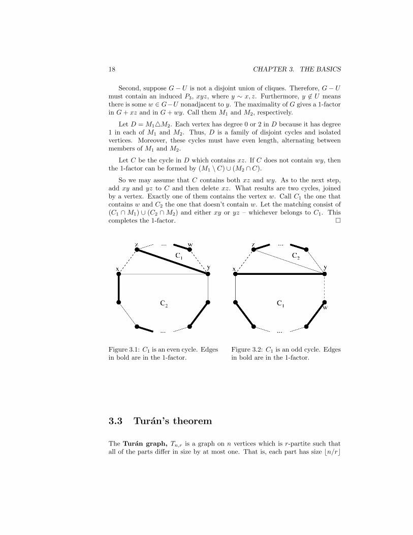
So we may assume that C contains both xz and wy. As to the next step,add xy and yz to C and then delete xz. What results are two cycles, joinedby a vertex. Exactly one of them contains the vertex w. Call C1 the one thatcontains w and C2 the one that doesn’t contain w. Let the matching consist of(C1 ∩M1) ∪ (C2 ∩M2) and either xy or yz – whichever belongs to C1. Thiscompletes the 1-factor.

Figure 3.1: C1 is an even cycle. Edgesin bold are in the 1-factor.

Figure 3.2: C1 is an odd cycle. Edgesin bold are in the 1-factor.

3.3 Turan’s theorem

The Turan graph, Tn,r is a graph on n vertices which is r-partite such thatall of the parts differ in size by at most one. That is, each part has size bn/rc

3.3. TURAN’S THEOREM 19

or dn/re. The Turan number tn,r = |Tn,r| is

tn,r =

(n

2

)− (n− rbn/rc)

(dn/re

2

)− (r (bn/rc+ 1)− n)

(bn/rc

2

)=

(1− 1

r

)n2

2− r

2

(⌈nr

⌉− n

r

)(nr−⌊nr

⌋)≥

(1− 1

r

)n2

2− r

8

and, of course,

tn,r ≤(

1− 1

r

)n2

2.

The typical formulation of Turan’s theorem [Tur41] is that the maximumnumber of edges in a graph with no copy of Kr+1 is tn,r. There’s a strongerstatement and proof due to Erdos [Erd70] from 1970. A sequence a1 ≥ a2 ≥· · · ≥ an is said to majorize b1 ≥ b2 ≥ . . . ≥ bn if ai ≥ bi for i = 1, . . . , n.

Theorem 3.3.1 (Turan [Tur41]) Let G be a simple graph on n vertices withno copy of Kr+1 and degree sequence d1 ≥ d2 ≥ · · · ≥ dn. There exists an r-partite graph on n vertices whose degree sequence majorizes the degree sequenceof G.

Proof. The proof proceeds by induction on r and the case r = 1 is trivial. Letr ≥ 1 and G be a graph on n vertices with no copy of Kr+1 and degree sequenced1 ≥ d2 ≥ · · · ≥ dn. Let v1 be a vertex of maximum degree, d1. If vi ∈ N(vn)has degree di, then let d′i = |N(vi) ∩N(v1)|. Note that di − d′i ≤ n− |N(v1)|.

Since G[N(v1)] has no copy of Kr, the inductive hypothesis gives that there isan (r−1)-partite graph G′ on |N(v1)| vertices whose degree sequence majorizesthat of G[N(v1)]. In particular, the vertex corresponding to vi has degree atleast d′i in G′. Construct G′′ by appending n−|N(v1)| vertices to G′, connectingeach of them to the vertices in G′.

The vertices not in G′ have degree d1, which is the largest degree-value in G.The vertex in G′ corresponding to vi has degree, in G′′, at least d′i+n−|N(v1)| ≥di.

Therefore, G′′ is an r-partite graph whose degree sequence majorizes that ofG.

Exercises.

(1) Prove that Tn,r is the n-vertex r-partite graph with the most number ofedges.


3.4 Konigsberg

The famous bridges of Konigsberg2 problem asked if one could traverse thebridges of Konigsberg exactly once and return to the same point. Euler provedthat it was impossible in 1741 and stated, without proof, that the necessarycondition was sufficient. A history of the Konigsberg problem can be found inWilson [Wil86]. An Eulerian circuit of a graph G is a circuit (i.e., a closedtrail) that contains all the edges of G. A graph with an Eulerian circuit is calledan Eulerian graph. An Eulerian trail is a trail that contains all the edgesof G. The proof of Theorem 3.4.1 is due to Hierholzer and Weiner [HW73].

Theorem 3.4.1 A graph G has an Eulerian circuit iff all vertex degrees areeven and all edges belong to a single component.

A graph G has an Eulerian trail iff G all but 2 vertex degrees are even andall edges belong to a single component.

Proof. The even-degree condition for an Eulerian circuit is clearly necessary.So suppose G is a graph with all even vertex degrees and all edges belonging to asingle component and G has at least one edge. Let T be a maximum-length trailin G. It must be a maximal trail and must be a circuit because the endverticesof T must be saturated in T and if they are not the same vertex, then theirdegrees are odd, a contradiction.

Let G′ = G−E(T ). Since T is a circuit, G′ has all even degrees. If E(G′) isnonempty, then the vertex set of each nontrivial component of G′ must intersectwith the vertex set of C. So, there is some uv ∈ E(G′) that is incident to avertex v ∈ V (C). So, T + uv is a trail, which can be seen by beginning with uand then traversing the circuit T , beginning and ending at v. Thus, T +uv is alonger trail than T , a contradiction. Therefore, the first part of Theorem 3.4.1is proved.

As to the existence of an Eulerian trail, this is easy, given the previous part.Let x and y be the odd-degree vertices. The graph G+xy is Eulerian. Constructits Eulerian circuit C and so C − xy is the Eulerian trail.

3.5 Dirac’s theorem

A Hamilton cycle in a graph G is a cycle that contains every vertex. A graphis Hamiltonian if it contains a Hamilton cycle.

Theorem 3.5.1 (Dirac [Dir52]) If G is a simple graph on n ≥ 3 verticeswith minimum degree at least n/2, then G is Hamiltonian.

Ore [Ore60] stated that if deg(u) + deg(v) ≥ n for all nonadjacent verticesu and v, then the graph is Hamiltonian iff G + uv is Hamiltonian. Combining

2This is now the city of Kaliningrad, Russia, a province noncontiguous with the rest of thecountry.

3.6. THE HAJNAL-SZEMEREDI THEOREM 21

these, we can prove the following generalization of Dirac. Note that the caseof K2, which fulfills the minimum degree condition but is not Hamiltonian isexcluded by Theorem 3.5.2.

Theorem 3.5.2 (Ore [Ore60]) If G is a simple graph on n vertices such thatdeg(u) + deg(v) ≥ n for all nonadjacent u and v, then G is Hamiltonian.

Proof. The degree condition gives that G is connected. (In fact, it gives thatthe diameter of G is at most 2.) Let P = v1, . . . , vk be a maximum-sized pathin G. If vk ∼ v1, then v1, . . . , vk is a cycle and, since G is connected, if G is notHamiltonian, then there is some vertex not on the cycle adjacent to a vertex onthe cycle. This contradicts the maximality of P .

Since v1 6∼ vk, deg(v1) + deg(vk) ≥ n, but since P is maximal, all of theneighbors of v1 and of vk are in P . Let T be the set of neighbors of vk and letS be the predecessors of the neighbors of v1. That is, vi ∈ S iff vi+1 ∼ v1. Notethat S ⊆ v1, . . . , vk−2 and T ⊆ v2, . . . , vk−1. Since k ≤ n, |S ∪ T | ≤ n − 1but |S| + |T | ≥ n. So, S ∩ T 6= ∅. Let vj ∈ S ∩ T . So, v1 ∼ vj+1 and vk ∼ vj .The vertices

vj , vj−1, . . . , v1, vj+1, vj+2, . . . , vk, vj

form a cycle. Since P was maximum-sized and G is connected, k = n and wehave exhibited the Hamilton cycle.

Exercises.

(1) For each n, find two examples of connected graphs with minimum degreeat least dn/2e − 1 which are not Hamiltonian.

(2) Prove that if G is a simple graph on n vertices with minimum-degree atleast n/2, then G contains a matching (1-regular subgraph) with bn/2cedges.

(3) Prove that, if G is a simple graph with minimum degree at least n/2 thenthere exists a matching with bn/2c edges.

3.6 The Hajnal-Szemeredi theorem

An equitable k-coloring of a graph G is a proper coloring of G in k colorssuch that any two color classes differ in size by at most 1.

In 1963, Corradi and Hajnal [CAH63] proved that, for every graph G withmaximum degree ∆(G) ≥ 2, then G has an equitable 3-coloring. In 1964, Erdosconjectured that any graph with maximum degree ∆(G) ≤ r has an equitable(r + 1)-coloring.

It is easy to see that this is best possible. Let G be a graph that containsan (r + 2)-clique. No matter what the rest of the graph is, even though it canbe chosen so that ∆(G) = r+ 1, G cannot admit any (r+ 1)-coloring, let alonean equitable one.


In 1970, Hajnal and Szemeredi [HS70] proved Erdos’ conjecture to be correct,although their argument is rather complicated. The proof presented here is dueto Kierstead and Kostochka [KK08]. Before we prove the theorem itself, wenote that the complementary version is often the form used.

Theorem 3.6.1 (Hajnal-Szemeredi [HS70] – complementary form) If Gis a simple graph on n vertices with minimum degree δ(G) ≥ k−1

k n, then G con-tains a subgraph that consists of bn/kc vertex-disjoint copies of Kk.

The statement of Hajnal-Szemeredi is exactly that of Erdos’ conjecture:

Theorem 3.6.2 (Hajnal-Szemeredi [HS70]) If G is a simple graph on nvertices with maximum degree ∆(G) ≤ r, then G has an equitable (r + 1)-coloring.

Proof. We may assume that n is divisible by r + 1 because if p = n − (r +

1)⌊

nr+1

⌋, then any equitable coloring of G + Kp induces an equitable coloring

of G.So, let G be a graph on s(r + 1) vertices with maximum degree r. We say

that G has a nearly equitable (r + 1)-coloring, which is a proper coloringc such that all color classes have size s except one V +(c), of size s + 1, andanother V −(c), of size s− 1.

The proof of the theorem is in two parts. Part I describes the importantproperties of a nearly equitable (r + 1)-coloring. Part II shows that our graphG may be assumed to have such a coloring and uses Part I to complete the proof.

Part I. Properties of a nearly equitable coloring. Given a nearly-equitable coloring c, let D = D(G, c) be an auxiliary digraph whose verticesare the color classes3 of G under c and an arc (X,Y ) belongs to A(D) iff somevertex x ∈ X has no neighbors in Y .

Such a vertex x is said to be movable to Y . If there exists a directed pathin D from X to V −, then X is called accessible. We also define V − to betrivially accessible. If V + is accessible, it is an easy exercise to see that theproof is finished:

Lemma 3.6.3 If G has a nearly equitable (r + 1)-coloring c, for which V +(c)is accessible, then G has an equitable (r + 1)-coloring.

The family of accessible classes is denoted A(c), A :=⋃A and the family of

inaccessible classes is denoted B(c), B := V (G) − A. Let m be the number ofaccessible classes that are not V −. Let q be the size of B; i.e., q is the numberof inaccessible classes. That is,

m := |A| − 1 and q := r −m.3In order to avoid confusion, we will refer to the vertices of D as “classes”. The vertices

of G will be lowercase Latin letters and the classes of D will be uppercase Latin letters.


Consequently,

|A| = ms+ (s− 1) and |B| = qs+ 1.

No vertex b ∈ B can be moved to A and so b must be adjacent to at least onevertex in every class of A:

degA(b) ≥ m+ 1 =⇒ degB(b) ≤ q − 1 for all b ∈ B. (3.3)

If V − is the only accessible set, then m = 0, q = r and

e(A,B) ≤ r|V −| = r(s− 1) < rs+ 1 = |B|,

contradicting the first inequality of (3.3).So we may assume that 2 ≤ m + 1 = |A|. Call a class Y ∈ A terminal if

V − is reachable from every class X ∈ A− Y in the digraph D − Y . In otherwords, class Y is terminal if, for every accessible class X, there is a directedpath from X to V − that does not involve Y . Since m ≥ 1, we can define V − tobe non-terminal.

Every non-terminal X partitions A−X into SX and TX 6= ∅ where SX isthe set of classes that are reachable from V − in D −X. Observe that there isno arc from TX − X to SX .

Choose some non-terminal class U so that A′ := TU 6= ∅ is minimal. Thenevery class in A′ is terminal, otherwise some class U ′ ∈ TU could have beenchosen rather than U . If that were the case, then SU ⊇ SU∪U. See Figure 3.3.Set t := |A′| and A′ =

⋃A′. Since there are no classes in A′ that point to a

Figure 3.3: Diagram of the digraph D. The class U is a non-terminal class suchthat TU is minimal. |A′| = t, |SU | = m− t, |B| = q = r −m.

class in A − (A′ ∪ U), every vertex in A′ must be adjacent to at least onevertex in each color class in A− (A′ ∪ U). Therefore,

degA(a) ≥ m− t for all a ∈ A′. (3.4)


Let ab be an edge with a ∈ W ∈ A′ and b ∈ B. We call ab a solo edgeif NW (b) = a. The endvertices of solo edges are solo vertices and verticeslinked by solo vertices are called special neighbors of each other. Let Sadenote the special neighbors in B of a ∈ A′ and Sb denote the set of specialneighbors in A′ of b ∈ B. Because b must be adjacent to at least one vertex ineach member of A, the number of color classes in A in which b has at least twoneighbors is at most r− (m+ 1 + degB(b)). Consequently, we can lower boundthe number of vertices that are special neighbors of b ∈ B:

|Sb| ≥ t− (r −m− 1− degB(b)) = t− q + 1 + degB(b). (3.5)

Lemma 3.6.4 If there exists W ∈ A′ such that no solo vertex in W is movableto a class in A−W, then q+ 1 ≤ t. Furthermore, every vertex b ∈ B is solo.

Proof. Let W1 be the set of solo vertices in W and W2 := W −W1. Everyvertex in B is adjacent to at least one vertex in W . Furthermore, every vertexin B − NB(W1) is adjacent to at least two vertices in W . Therefore,

e(W,B) ≥ 2|B| − |NB(W1)| = 2(qs+ 1)− q|W1| = qs+ q|W2|+ 2.

No vertex inW1 can be moved to another class inA. So, degB(x) ≤ r−m = qfor all x ∈W1. By (3.4), degB(w) ≤ r − (m− t) = q + t for all w ∈W . So,

qs+ q|W2|+ 2 ≤ e(W,B) ≤ q|W1|+ (t+ q)|W2| ≤ qs+ t|W2|

and it follows that t ≥ q + 1. Furthermore, according to (3.5), if b ∈ B, then

|Sb| ≥ t− q + 1 + degB(b) ≥ t− (t− 1) + 1 + degB(b) ≥ 2.

Since b has at least 2 special neighbors, it must be a solo vertex.

Lemma 3.6.5 There exists a solo vertex z ∈ W ∈ A′ such that either z ismovable to a class in A − W or z has two nonadjacent special neighbors inB.

Proof. Assume, by way of contradiction, the lemma is not true. By Lemma 3.6.4,every vertex in B is a solo vertex and Sz, the set of special neighbors of z, inducesa clique for every solo z ∈W . Let µ be defined on E(A′, B) as follows:

µ(xy) :=

q|Sx| , if xy is a solo edge;

0, otherwise.

As a result, for z ∈ A′, it is the case that µ(z,B) :=∑b∈B µ(zb) = |Sz| q|Sz| =

q if z is a solo vertex and µ(z,B) = 0 otherwise. Trivially, µ(A′, B) :=∑z∈A µ(z,B) ≤ q|A′| = qst.Now we count µ(A′, B) by summing over the second coordinate. Let b ∈ B

and cb := max|Sz| : z ∈ Sb Recall that Sz is a clique and use the bound on


the right hand side of (3.3), to obtain cb − 1 ≤ degB(b) ≤ q − 1. Therefore,cb ≤ q and along with (3.5), we have

µ(A′, b) =∑z∈Sb

q

|Sz|≥ |Sb| q

cb≥ (t− q + cb)

q

cb= (t− q) q

cb+ q ≥ (t− q) + q = t.

Therefore,

µ(A′, B) ≥ t|B| = t(qs+ 1) > qst ≥ µ(A′, B),

a contradiction.

Part II. Proof of the theorem. To prove the Hajnal-Szemeredi theoremitself, we proceed by a triple induction. The first induction is on r, the secondis on e(G) and the third is on q, the number of non-accessible classes of a givennearly-equitable coloring.

The base case of the induction on r, r = 0, is trivial, the empty graph has a1-coloring.

The second induction is on e(G). The base case e(G) = 0 is likewise trivial,so suppose the theorem is true for e(G) − 1. Let xy be an edge of G. By theinduction hypothesis there is an equitable (r + 1)-coloring of G − xy. We aredone unless there is a color class V with both x and y. The fact that deg(x) ≤ rgives that there is some color class W such that x is movable to W . This givesa nearly equitable coloring c of G. Let V − = V − x and V + = W ∪ x.

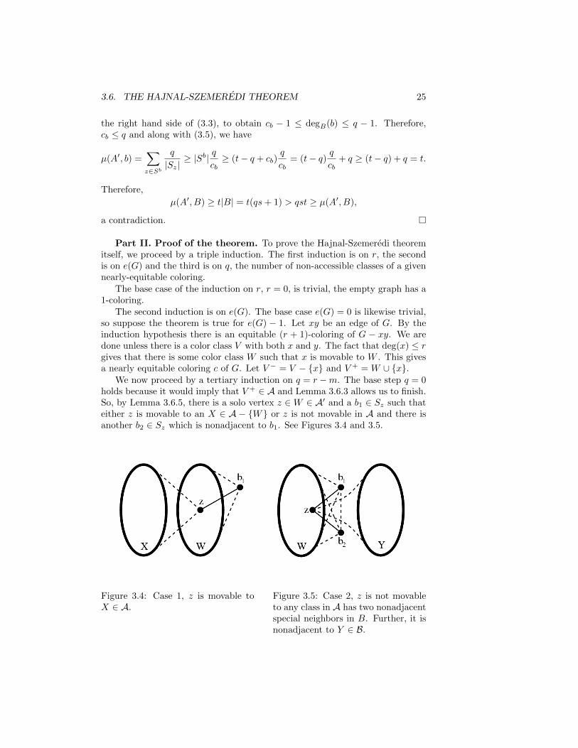
We now proceed by a tertiary induction on q = r −m. The base step q = 0holds because it would imply that V + ∈ A and Lemma 3.6.3 allows us to finish.So, by Lemma 3.6.5, there is a solo vertex z ∈W ∈ A′ and a b1 ∈ Sz such thateither z is movable to an X ∈ A − W or z is not movable in A and there isanother b2 ∈ Sz which is nonadjacent to b1. See Figures 3.4 and 3.5.

Figure 3.4: Case 1, z is movable toX ∈ A.

Figure 3.5: Case 2, z is not movableto any class in A has two nonadjacentspecial neighbors in B. Further, it isnonadjacent to Y ∈ B.


We use the first induction hypothesis and (3.3) on B− := B − b1. Recall|B−b1| = qs. Since ∆(G[B−]) ≤ q− 1 < r, this gives an equitable q-coloring– denoted g – of B−. Set A+ := A ∪ b1.

Case 1: z is movable to X ∈ A.Move z to X and b1 to W −z to obtain a nearly equitable (m+1)-coloring, γ,of A+. See Figure 3.4. Since W ∈ A′(c), V +(γ) = X ∪z ∈ A(γ). But, V +(γ)is accessible, so Lemma 3.6.3 gives that A+ has an equitable (m + 1)-coloringγ′. Combine this with the equitable coloring g of B− and we see that γ′ ∪ g isan equitable (r + 1)-coloring of G.

Case 2: z is not movable to any class in A.In this case, degA+(z) = degA(z) + 1 ≥ m+ 1 and so degB−(z) ≤ r− (m+ 1) =q − 1. Therefore, there is a color class under g, Y ∈ B−(g) to which z can beadded to get a new coloring f ′ of B∗ := B ∪ z − b1. Also move b1 to W toobtain a (m+ 1)-coloring ϕ of A∗ := V (G)−B∗. See Figure 3.5.

Combine these colorings to obtain ϕ′ = ϕ ∪ f ′. Not only is ϕ′ an nearlyequitable coloring of G but also W is terminal, so every class in A\W is stillaccessible. Since z was not movable but W was itself accessible, the new classW ∗ := W ∪ b1 − z is accessible. Even more, b2 is movable to W ∗, so theclass of ϕ′ to which it belongs is also accessible. So, q(ϕ′) < q(c) and by thethird induction, G has an equitable (r + 1)-coloring.

Exercises.

(1) Prove Lemma 3.6.3.

(2) Prove the complementary form of Hajnal-Szemeredi, using the originalform.

3.7 Gems: The Hoffman-Singleton theorem

The Hoffman-Singleton theorem is one of the most elegant theorems in extremalgraph theory. It is an ideal example of the application of linear algebraic meth-ods.

The diameter of a graph G is the largest distance between two vertices andthe girth is the length of the shortest cycle. Clearly, an r-regular graph withdiameter d has at most 1 + r

∑d−1i=0 (r − 1)i vertices.

The girth of a graph G is the length of the shortest cycle. Clearly anr-regular graph with girth 2d+ 1 has at most 1 + r

∑d−1i=0 (r − 1)i vertices.

Hoffman and Singleton [HS60] defined a Moore graph to be an r-regular

graph that has diameter d and exactly 1 + r∑d−1i=0 (r − 1)i vertices. We leave

as an exercise that this is equivalent to having girth 2d + 1 and exactly 1 +r∑d−1i=0 (r − 1)i vertices. Singleton [Sin68] proved later that there can be no

irregular graph with diameter d and girth 2d+ 1:

3.7. GEMS: THE HOFFMAN-SINGLETON THEOREM 27

Theorem 3.7.1 (Singleton [Sin68]) Let d be a positive integer and G be agraph with diameter d and girth 2d+ 1. Then there is a positive integer r suchthat G is r-regular.

The theorem of Hoffman and Singleton proved that, in fact, there cannot bemany Moore graphs. They proved that none can exist for d ≥ 4 and for d = 3,must be a 7-cycle. As for d = 2, they proved the following astounding result.

Theorem 3.7.2 (Hoffman-Singleton [HS60]) Let G be an r-regular, diameter-2 graph on r2 + 1 vertices. Then r ∈ 2, 3, 7, 57.

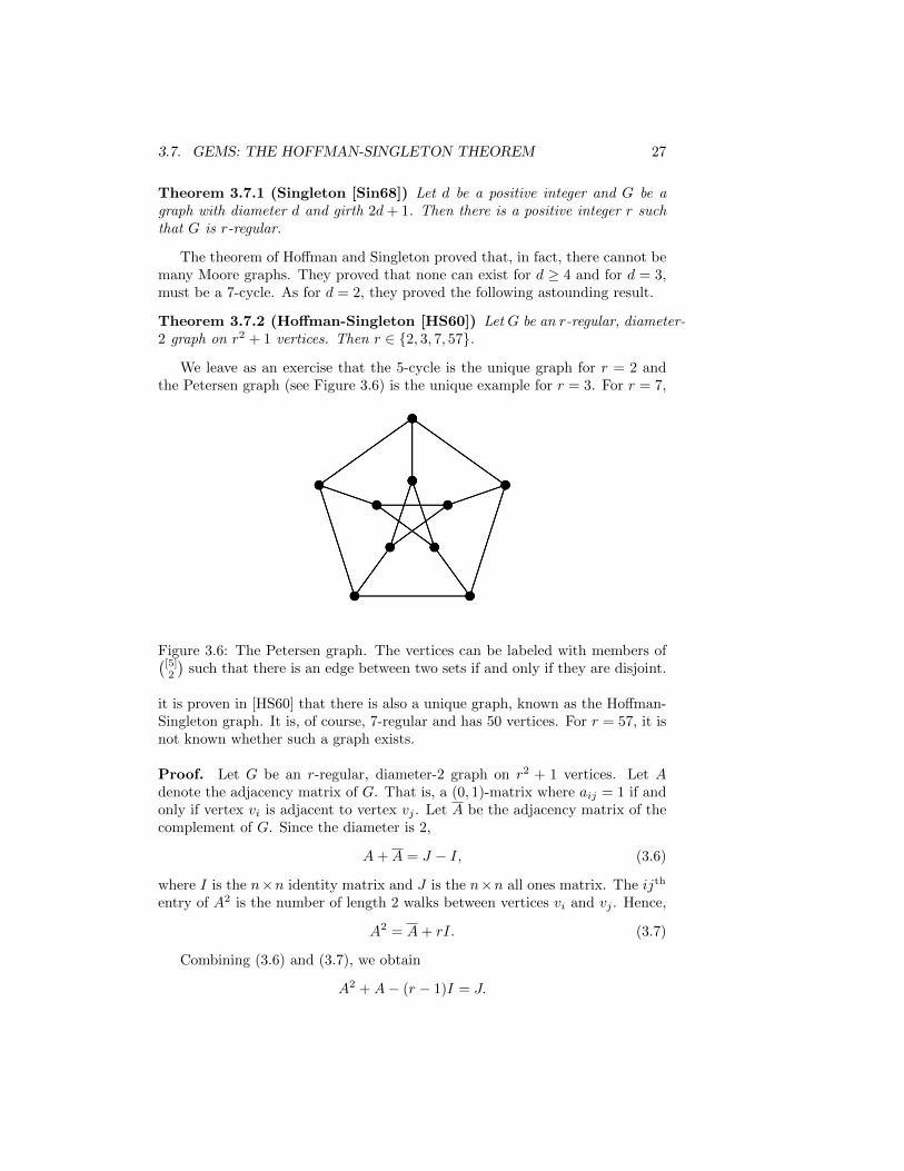
We leave as an exercise that the 5-cycle is the unique graph for r = 2 andthe Petersen graph (see Figure 3.6) is the unique example for r = 3. For r = 7,

Figure 3.6: The Petersen graph. The vertices can be labeled with members of([5]2

)such that there is an edge between two sets if and only if they are disjoint.

it is proven in [HS60] that there is also a unique graph, known as the Hoffman-Singleton graph. It is, of course, 7-regular and has 50 vertices. For r = 57, it isnot known whether such a graph exists.

Proof. Let G be an r-regular, diameter-2 graph on r2 + 1 vertices. Let Adenote the adjacency matrix of G. That is, a (0, 1)-matrix where aij = 1 if andonly if vertex vi is adjacent to vertex vj . Let A be the adjacency matrix of thecomplement of G. Since the diameter is 2,

A+A = J − I, (3.6)

where I is the n×n identity matrix and J is the n×n all ones matrix. The ijth

entry of A2 is the number of length 2 walks between vertices vi and vj . Hence,

A2 = A+ rI. (3.7)

Combining (3.6) and (3.7), we obtain

A2 +A− (r − 1)I = J.


Now let us consider the eigenvalues and eigenvectors. The all-ones vector 1 isan eigenvector of A corresponding to eigenvalue r because the regularity of G.That is, A~1 = r~1. Let ~1, v2, . . . , vn be a set of pairwise orthogonal eigenvectors.

If vi, i ≥ 2 is an eigenvector of A corresponding to eigenvalue λ, then J~1 = ~0.

A2~vi +A~vi − (r − 1)I~vi = J~vi

(λ2 + λ− (r − 1))~vi = ~0

Since eigenvectors cannot be ~0, we have λ = (−1±√

4r − 3)/2, neither of whichis r.

Let m1 and m2 be the multiplicities of λ1 = (−1 −√

4r − 3)/2 and λ2 =(−1 +

√4r − 3)/2, respectively. Since r has multiplicity 1,

1 +m1 +m2 = n = r2 + 1. (3.8)

Since the sum of the eigenvalues is equal to the trace, tr(A) = 0 and

r +m1λ1 +m2λ2 = 0

r +m1

(−1

2−√

4r − 3

2

)+m2

(−1

2+

√4r − 3

2

)= 0

2r − (m1 +m2) + (m2 −m1)√

4r − 3 = 0

2r − r2 +√

4r − 3(m2 −m1) = 0, (3.9)

using (3.8).Let s =

√4r − 3. Observe that since s is the square root of an integer,

it is either irrational or a positive integer. In the case where s is irrational,m1 −m2 = 0 and (3.9) implies r = 2: the 5-cycle.

So we may assume that s is an integer. Substitute 4r − 3 = s2 into (3.9):

2

(s2 + 3

4

)−(s2 + 3

4

)2

+ s(m2 −m1) = 0

s4 − 2s2 + 16(m1 −m2)s− 15 = 0. (3.10)

The only integer solutions of (3.10) must divide 15 and, since s is positive, wehave that s ∈ 1, 3, 5, 15, implying r ∈ 1, 3, 7, 57. The case r = 1 is a match-ing and cannot be a radius 2 graph. Combining this with the case where s isirrational, the only possible values of r are in 2, 3, 7, 57.

Babai and Frankl [BF92] refer to Theorem 3.7.2 in the section appropriatelyentitled “Beauty is Rare” and our proof is similar to theirs, although the originalproof of Hoffman and Singleton is not substantially different.

Going back through the Hoffman-Singleton proof, we can derive that thespectrum of A for the missing Moore graph is 571(−8)152071729 (multiplicitiesare in the exponent). Higman (see [Cam99]) proved that the missing Mooregraph cannot be vertex-transitive. Macaj and Siran [MS] proved further thatthe automorphism group of the missing Moore graph must have order at most

3.7. GEMS: THE HOFFMAN-SINGLETON THEOREM 29

375. Compare this to the Hoffman-Singleton graph, whose automorphism grouphas order 252, 000 [Haf03].

Exercises.

(1) Prove that the following are equivalent:

(a) G is r-regular with diameter d and has exactly 1 + r∑d−1i=0 (r − 1)i

vertices.

(b) G is r-regular with girth 2d + 1 and has exactly 1 + r∑d−1i=0 (r − 1)i

vertices.

(2) Prove that the 5-cycle is the unique Moore graph of degree 2 and that thePetersen graph is the unique Moore graph of degree 3.


Chapter 4

Ramsey Theory

4.1 Basic Ramsey theory

The basic graph version of Ramsey’s theorem is that, given positive integers kand l, there is an n = R(k, l) such that if E(Kn) are colored red and blue, thereis other a red Kk or a blue Kl.

Definition 4.1.1 The family of r-sets of a set S is denoted(Sr

). A q-coloring

of(Sr

)is a function f :

(Sr

)→ [q]. A homogeneous set T is a subset T ⊆ S

for which each set in(Tr

)is the same color. We say T is i-homogeneous if all

of its sets receive color i.The notation n → (s1, . . . , sq)

r means that, for every q-coloring of(

[n]r

),

there exists an i ∈ [q] such that there is an i-homogeneous set of size si.The notation R(k, l) is the least number n such that n→ (k, l)2.

Theorem 4.1.2 (Ramsey [Ram30]) For positive integers q, r and s1, . . . , sq,there exists an integer n such that n→ (s1, . . . , sq)

r.

The proof proceeds by a double induction on r and then∑i si. We neglect

the general proof in favor of concentrating on the graph Ramsey bound.

Theorem 4.1.3 If k, l ≥ 2 and n ≥(k+l−2k−1

), then n→ (k, l)2.

That is, R(k, l) ≤(k+l−2k−1

).

Proof. We proceed by induction on k + l. It is easy to see that R(k, 2) = kand R(2, l) = l, which suffices for a base case.

Suppose the statement of the theorem is true for k + l − 1.Let n = R(k, l)− 1 and color the edges of Kn such that there is no blue Kk

or red Kl. Choose any vertex v. The red neighborhood of v has size at mostR(k − 1, l) − 1, otherwise either this neighborhood has a blue l-clique or thered neighborhood has a red (k − 1)-clique, a contradiction. Similarly, the blueneighborhood of v has size at most R(k, l − 1)− 1.

31

32 CHAPTER 4. RAMSEY THEORY

Hence, R(k, l) − 2 = n − 1 ≤ (R(k − 1, l)− 1) + (R(k, l − 1)− 1) whichsimplifies to

R(k, l) ≤ R(k − 1, l) +R(k, l − 1) (4.1)

and the expression R(k, l) =(k+l−2k−1

)satisfies both (4.1) as well as the base

cases.

See the dynamic survey by Radziszowski [Rad94] for a summary of knownresults on Ramsey numbers. Much of the focus on interest in Ramsey theoryis on the so-called diagonal Ramsey numbers. That is, the numbers R(k, k).According to Stirling’s formula (see [Wei]), the binomial coefficient bound hasthe following asymptotic:

R(k, k) ≤(

2k − 2

k − 1

)= (1+o(1))

√2π(2k − 2)

(2k−2e

)2k−2(√2π(k − 1)

(k−1e

)k−1)2 =

1 + o(1)

4πk4k ≤ C√

k4k,

for some constant C.As to the lower bound on the diagonal Ramsey numbers, we leave that for

the next chapter.

Exercises.

(1) Prove the general form of Ramsey’s theorem.

4.1.4 Infinite Ramsey theory

The infinite version of Ramsey’s theorem is as follows:

Theorem 4.1.5 Given integers r, q and a coloring c :(Nr

)→ [q], there is an

infinite set M ⊆ N such that(Mr

)is monochromatic.

Proof. It is sufficient to prove Theorem 4.1.5 in the case where q = 2, we leavethis as an exercise. Note also that in the statement of the theorem, N can bereplaced by any countably infinite set.

The proof proceeds by induction on r. If r = 1, then the statement says thatif c : N→ [2], then there is an infinite monochromatic set, which is obvious.

Suppose, by way of induction, that for r ≥ 1, M ′ an infinite set and any

coloring c :(M ′

r

)→ [2], there is an infinite set M ′′ such that

(M ′′

r

)is monochro-

matic. Let c be a coloring of the (r + 1)-sets of N. Set Y0 = N.Choose x0 = 1. The coloring c of the (r + 1)-sets of Y0 induces a coloring

of the r-sets of Y0 by giving the set S the color c(x0 ∪ S). By the inductivehypothesis, there is a set Y1 ⊇ Y0 such that the r-sets of Y1 all get the samecolor by this derived coloring. Let x1 ∈ Y1.

Repeat this process to get x0, x1, x2, . . . with the property that if xi1 , . . . , xir+1

is an (r+1)-set with i1 < i2 < · · · < ir+1, then the color of this set only dependson i1. Since there are only 2 colors, one color occurs for an infinite subsequence

4.2. CANONICAL RAMSEY THEORY 33

of x0, x1, x2, . . . and so that subsequence is M .

Theorem 4.1.2 follows from Theorem 4.1.5. Theorem 4.1.5. Bollobas [Bol98]notes that this consequence is a special case of Tychonov’s theorem:Proof. Finite Ramsey from infinite Ramsey (s1 = · · · = sq = l).We are given Theorem 4.1.2 and we will suppose, by way of contradiction, thatTheorem 4.1.5 is false. Then there exists r, l, q such that for every integer n,there exists a c :

([n]r

)→ [q] such that there is no monochromatic set of size l.

For every integer n, let Cn be a nonempty set of k-colorings of(

[n]r

)such that

if n < m and cm ∈ Cm, then restricting of cm to(

[n]r

)(denote it to be cm|[n]) is

in Cn.For m > n, let Cn,m ⊆ Cn,m be the k-colorings that are restrictions of

colorings of Cm. Thus, Cn ⊃ Cn,m ⊃ Cn,m+1. For every n, we can define

Cn =def=

∞⋂m=n+1

Cn,m 6= ∅.

This is nonempty because each Cn,m is finite.

Thus, we can find cr ∈ Cr and choose cr+1 ∈ Cr+1, cr+2 ∈ Cr+2, . . . with theproperty that each is the restriction of the previous one. I.e., cn = cn+1|[n].

This now allows us to define a coloring c :(Nr

)→ [k] where, for any S ∈

(Nr

),

S receives the colorc(S) = cn(S) = cn+1(S) = · · ·

where n is the maximum element of S.

Exercises.

(1) Prove that Theorem 4.1.5 holds for an arbitrary q if it holds for q = 2.

4.2 Canonical Ramsey theory

Erdos and Rado [ER52] introduced the notion of canonical Ramsey theory.In the Ramsey theorem, the number of colors is fixed and if the system is suffi-ciently large, there is a monochromatic clique (in either the graph or hypergraphsense). The canonical version of Ramsey does not restrict the number of colorsbut still demonstrates that certain substructures are unavoidable.

Definition 4.2.1 For any pair of infinite sets N1, N2, positive integer r, andcolorings c1 :

(N1

r

)→ C1 and c2 :

(N2

r

)→ C2, we say c1 and c2 are equivalent

if there is a one-to-one map ϕ : N1 → N2 such that for e, e′ ∈(N1

r

), it is the

case that c1(e) = c1(e′) iff c2(ϕ(e)) = c2(ϕ(e′)).For any infinite set N , positive integer r, and coloring c :

(Nr

)→ C, we say

c is irreducible if for every infinite subset N1 of N , the restriction of c to(N1

r

)is equivalent to c.


A set C of colorings(Nr

)→ N is unavoidable if for every coloring c :

(Nr

)→

N, there is an infinite set M ⊂ N such that the restriction of c to(Mr

)is

equivalent to a member of C.

It is easy to construct some irreducible colorings of(Nr

). The monochromatic

and rainbow colorings are irreducible. For any S ∈ [r], define the S-canonicalcoloring cS :

(Nr

)→(N|S|)

such that cS(e) = eS , where eS = ei : i ∈ S.Observe that c∅ is the monochromatic coloring and c[r] is the rainbow col-

oring. Further, observe that there are four canonical colorings when r = 2. Inthat case, we can denote c1(ij) = i and c2(ij) = j.

4.2.2 Infinite version

Let N be an infinite set and recall that, for a positive integer r,(Nr

)denotes

the set of r-subsets of N . The general canonical Ramsey theorem is stated asfollows:

Theorem 4.2.3 (Erdos-Rado, [ER52]) Let r be a positive integer and c :(Nr

)→ N be a coloring. Then there is an infinite set M ⊆ N such that the

restriction of c to(Mr

)is canonical.

A very nice proof of this theorem is given in Bollobas’ Modern Graph The-ory [Bol98]. We will show the proof for r = 2, the general proof is not muchmore difficult.Proof. r = 2.Let c be a coloring of

(N2

). There are only a finite number of possible patterns

of(

[4]2

), so by the infinite version of Ramsey’s theorem, there is an infinite set

M such that all 4-sets of M receive the same pattern.We shall prove that the restriction of c to

(M2

)is canonical. If c 6= c[2], then

there are two edges with the same color. Suppose c(mimj) = c(mkml) withmi 6∈mj ,mk. We cannot assume i < j or i > j. Then c(m2im2j) = c(m2km2l) and

c(m2km2l) = c(m2i+1m2j). Thus,(M2

)has two adjacent edges of the same color.

Case 1. c(mimj) = c(mimk) for some i < j < k.By considering mi,mj ,mk,mk+1, the edges 12 and 13 get the same color andso any pair of edges sharing their first vertices get the same color. Thus, thereis a coloring d : M → N such that if r < s, then c(mrms) = d(mr).

Case 2. c(mimk) = c(mjmk) for some i < j < k.Similarly to Case 1, there is a coloring d : M → N such that if r < s, thenc(mrms) = d(ms).

Case 3. c(mimj) = c(mjmk) for some i < j < k.So, c(m1m3) = c(m3m5) and c(m2m3) = c(m3m4). Hence, there are edges ofthe same color sharing their first vertices and edges of the same color sharingtheir second vertices. Therefore, there are maps d1 : M → N and d2 : M → Nsuch that if i < j then c(mimj) = d1(mi) = d2(mj). Hence, any two edges havethe same color and c = c∅.

4.2. CANONICAL RAMSEY THEORY 35

If Case 3 holds, of course c = c∅. If Case 1 holds and Case 3 does not, thenc = c1. If Case 2 holds and Case 3 does not, then c = c2.

4.2.4 Canonical Ramsey numbers

The finite version of canonical Ramsey can be expressed as follows: Given in-tegers r and l, what is the minimum value of n such that any coloring

([n]r

)has a canonical coloring on some subset of l integers? This number is denotedER(r; l), the Erdos-Rado numbers.

For graphs, there are only three canonical colorings as described above. Theyare monochromatic (the coloring c∅), rainbow (the coloring c1,2 which colorseach edge distinctly) and lexicographic (either of the colorings c1 or c2).Simply put, a lexicographic coloring of E(K`) is one such that there is an orderon the vertices v1, . . . , v` and the color of edge vivj is mini, j.

Let towk(l) denote a tower of k− 1 twos and an l in the last exponent. I.e.,

22···

2l

.

Theorem 4.2.5 (Lefmann-Rodl, [LR95]) Let r be a positive integer. Thenthere exist positive constants cr, Cr such that for all positive integers l withl ≥ l0(r) the following holds:

2c2·l2

≤ ER(2; l) ≤ 2C2·l2·log l

towr(cr · l2) ≤ ER(r; l) ≤ towr+1

(Crl2r−1

log l

)

The proof of the upper bound is not easy, but the lower bound is due to aprevious paper of Lefmann and Rodl [LR93].

In order to show this lower bound for r = 2, we need some results on Ramseynumbers. Denote n = Rq(r; l) to mean that n → (l, . . . , l︸︷︷︸

q

)r. That is, any

coloring of the r-sets of n with q colors yields a monochromatic set of orderl. The following theorem is due to several papers: Erdos-Rado [ER52], Erdos-Hajnal-Rado [EHR65] and Erdos-Hajnal [EH89].

Theorem 4.2.6 Let r, q be positive integers with r ≥ 3 and q ≥ 2. Then thereexist positive constants cr,q, Cr,q such that if l ≥ l0(r),

Rq(r; l) ≤ towr(Cr,q · l)

Rq(r; l) ≥

towr(cr,q · l), if q ≥ 4;towr−1(cr,3 · l2 · log l), if q = 3;towr−1(cr,2 · l2), if q = 2.


The following theorem is due to several papers: Erdos, [Erd47], Erdos-Szemeredi, [ES72] and Lefmann, [Lef87].

Theorem 4.2.7 There exist constants c, C such that

2c·l·q ≤ Rq(2; l) ≤ 2C·l·q·log q

for all l ≥ 3.

To prove the lower bound of Theorem 4.2.5, we need the following claim:

Claim 4.2.8 ER(r; l) ≥ Rl−r(r; l).

Proof. First some notation: If S = s1, . . . , sr is an ordered set (s1 < s2 <· · · < sr)and I ⊆ [r], then S|I = si : i ∈ I.

Let n = Rl−r(r; l) − 1 and c :(

[n]r

)→ [l − r] be a coloring that has no

monochromatic l-subset of [n]. Suppose there is an l-subset X ⊆ [n] which hasa canonical coloring of

(Xr

). In order for this to happen, there must be a set

I ⊆ [r], I 6= ∅ such that c(S) = c(T ) iff S|I = T |I . Since c only has l− r colors,no such canonical coloring can exist because it would require at least l − r + 1colors.

All that remains is the monochromatic coloring, which is impossible becausec has no monochromatic l-subset of [n].

Using the fact that Rq(2; l) ≥ 2c3·l·q for all positive integers l ≥ 3 where c3is a positive constant. Claim 4.2.8 gives that ER(2; l) ≥ Rl−2(2; l) ≥ 2c

′·l2 forsome constant c′.

Exercises.

(1) For any S ∈ [r], prove that the S-canonical coloring is an irreduciblecoloring.

(2) Prove that ER(1; l) = (l− 1)2 + 1. Lefmann and Rodl say that this resultis folklore.

Chapter 5

The Power of Probability

Some of the most useful techniques in extremal graph theory are probabilistic innature. Sometimes the use of probability is explicit, sometimes it is implicit. Animportant resource on this methodology is the text of Alon and Spencer [AS00].

We will try to rely on an intuitive understanding of probability, but we willpresent the formal definitions because readers who are familiar with analysiswill find them enlightening and would provide some additional context.

5.1 Probability spaces

5.1.1 Formal definitions

In the most general setting, a probability space, Ω, is a measure space withmeasure Pr, such that Pr(Ω) = 1. An outcome in the probability space Ω issome ω ∈ Ω. An event in Ω is a subset A ⊆ Ω. We say that a sequence ofevents A1, A2, . . . occurs with high probability (whp) if limn→∞ Pr(An) = 1. Arandom variable X is a bounded, measurable function on Ω and, unless oth-erwise stated, is real-valued. That is, X : Ω→ R. The distribution functionof real-valued random variable X, is F (x) = Pr(X ≤ x). Two random variablesare said to have the same distribution if they have the same distributionfunction.

A probability mass function of a random variable X pi is a function of thereal numbers with a countable domain D such that

∑i∈D pi = 1. A probability

density function p(x) over the reals is a nonnegative-valued function such that∫∞−∞ p(y) dy = 1. Note that F (x) =

∫ x−∞ p(y) dy is a distribution function. In

this chapter, we will use something similar to the usual set theory notation forprobability. For example, if A1 and A2 are events, then the common event isdenoted A1 ∩A2. It is usual in probability to denote this as A1 ∧A2.

37

38 CHAPTER 5. THE POWER OF PROBABILITY

5.1.2 Probability in a discrete setting

The formal setting is not necessary for our understanding. We often use adiscrete random variable, which can be viewed as a countable (usually finite)number of values in a range space, say xii≥1. Each value has a probabilityassociated with it, denoted Pr(xi). For this to be a probability space, it isrequired that

∑i Pr(xi) = 1. The function p(i) = Pr(xi) is a probability mass

function. An event is simply a possible outcome. or a subset of the possiblevalues. The probability of event A is simply the sum of the probabilities of theindividual possible outcomes. For example, if A = X ∈ x2, x3, x5, thenPr(A) = Pr(X = x2) + Pr(X = x3) + Pr(X = x5).

For our purposes, almost every random variable will be a discrete randomvariable, although the careful and diligent reader can prove all of the theoremsusing measure theory.

5.1.3 Mean and variance

The expectation or mean of real-valued random variable X is defined to beE[X] =

∫Ωx dPr, if the integral is finite. If X is a discrete random variable that

takes on values xi, i ≥ 1, then

E[X] =∑i

xi Pr(X = xi).

If we say that “X is a random variable with mean µ,” this will imply that µexists and is finite. We can compute E[f(X)] for any f that makes the followingsummation finite:

E[f(X)] =∑i

f(xi) Pr(X = xi).

This kind of notation will be useful in random graph theory because the randomvariables themselves are graph-valued, but f will be a real-valued function.

If A is an event, we denote 1A to be the indicator variable of A. That is1A = 1 if the outcome of the random experiment is in A and is zero otherwise.So, E [1A] = Pr(A).

For any random variable X with mean µ, the variance of X, Var(X) :=E[(X − µ)2

], provided such an expression is finite. Otherwise, Var(X) = ∞.

The proof of Proposition 5.1.4 is left as an exercise.

Proposition 5.1.4 Let X be a random variable with finite variance and a andb be real numbers. Then,

Var(aX + b) = a2Var(X).

5.1. PROBABILITY SPACES 39

5.1.5 Independence

Finally, we say that the events A1, . . . , An are (mutually) independent if

Pr

(∧i∈S

Ai

)=

n∏i∈S

Pr(Ai) ∀S ⊆ [n].

A weaker condition is that the events A1, . . . , An are pairwise independentif, for all distinct i, j ∈ [n],

Pr (Ai ∧Aj) = Pr(Ai) Pr(Aj).

A set of variables X1, . . . , Xn are independent if the events Xi ∈ Sii∈Iare independent for all subsets Si and all I ⊆ [n]. A set of variables X1, . . . , Xn

are pairwise independent if the events Xi ∈ Sii∈I are pairwise independentfor all subsets Si and all I ⊆ [n].

Exercises.

(1) Prove Proposition 5.1.4.

(2) Prove that, for a random variable X, E[X2] ≥ (E[X])2.

(3) Prove that, for discrete independent random variables X and Y , thatE[XY ] = E[X]E[Y ]. (Note: This is true even if the random variables arenot discrete.)

(4) Use the previous exercise to prove that if X1, . . . , Xn are pairwise inde-pendent random variables, then

Var

(n∑i=1

Xi

)=

n∑i=1

Var(Xi).

5.1.6 Expectation

The most basic fact of expectation is that there is an outcome that is at leastas large as E[X] and an outcome that is at most as small as E[X].

Proposition 5.1.7 If X be a real-valued random variable on a probability spaceand E[X] ≥ m, then Pr(X ≥ m) > 0. In the case of a discrete random variable,that means that there is an x ≥ m such that Pr(X = x) > 0.

Symmetrically, if E[X] ≤ m, then Pr(X ≤ m) > 0.

Proof. Suppose, by way of contradiction, that Pr(X ≥ m) = 0. There existsan ε > 0 such that Pr(X ≤ m− ε) ≥ 1/2. Then,

m ≤ E[X] ≤ (m− ε) Pr(X ≤ m− ε) +mPr(m− ε < X < m)

≤ m− ε/2,

a contradiction.


5.2 Linearity of expectation

There is surprising power in using the linearity of the expectation function. Weleave the proof of Proposition 5.2.1 as an exercise.

Proposition 5.2.1 Let a1, . . . , an be real numbers and X1, . . . , Xn be randomvariables on the same probability space. Then,

E[a1X1 + · · ·+ anXn] = a1E[X1] + · · ·+ anE[Xn].

In particular, if X =∑i 1Ai , then E[X] =

∑i Pr(Ai).

5.2.2 A lower bound for diagonal Ramsey numbers

In the previous chapter, we establish that an upper bound on the Ramseynumber R(k, k) is C√

k4k, for some constant C. The lower bound, first due to

Erdos [Erd47], is remarkably simple and is often cited as an early example ofthe probabilistic method.

Theorem 5.2.3 (Erdos [Erd47])

R(k, k) > (1− o(1))k

e√

2

(√2)k.

Proof. For each edge in Kn, color it red or blue, independently, with probabil-ity 1/2. Let X be the random variable representing the number of homogeneous

sets in this random coloring. I.e., for every S ∈(

[n]k

), X =

∑S 1S is monochromatic.

E[X] = E

∑S∈([n]

k )

1S is monochromatic

=

∑S∈([n]

k )

E[1S is monochromatic

]=

∑S∈([n]

k )

Pr (S is monochromatic)

≤(n

k

)21−(k2) ≤

(enk

)k21−(k2). (5.1)

If this expectation is less than 1, then there is a coloring of the edges, red andblue, with no homogeneous set of size k and, thus, R(k, k) > n.

For any fixed ε > 0, plugging n = (1−ε) ke√

22k/2 will result in the expression

in (5.1) beingless than 1, for k large enough.

There have been small improvements on the general bounds on R(k, k), theso-called diagonal Ramsey numbers, but there has not been movement since1947 on the following:

√2 ≤ lim inf

k→∞R(k, k)1/k ≤ lim sup

k→∞R(k, k)1/k ≤ 4.

5.2. LINEARITY OF EXPECTATION 41

5.2.4 Finding a dense bipartite subgraph

Before we begin, let us consider the following theorem:

Theorem 5.2.5 Let G be a simple graph with n vertices and e edges. There isa partition of the vertex set of G, say V (G) = A + B such that at least half ofthe edges of G have one endpoint in A and one endpoint in B.

Proof. (#1)A typical proof of this theorem is algorithmic in nature. Let G be a simplegraph and V (G) = A0 +B0 be a bipartition. Let e(A0, B0) denote the numberof edges with one endpoint in A0 and one endpoint in B0. If there exists av ∈ A0 such that |N(v) ∩ A0| > |N(v) ∩ B0|, then create a new bipartitionwhere A1 = A0 \ v and B1 = B0 ∪v. The number of edges between A1 andB1 is

e(A1, B1) = e(A0, B0)− |N(v) ∩B0|+ |N(v) ∩A0|.

As long as a partition (Ai, Bi) has a vertex whose neighborhood in its ownpart is larger than its neighborhood in the other part, then there is a partition(Ai+1, Bi+1) such that e(Ai+1, Bi+1) > e(Ai, Bi). Since e(Ai, Bi) ≤ e(G) for alli, this algorithm will terminate. Upon termination, there is a partition (A,B)such that either e(A,B) = e(G) or, for every vertex a ∈ A, |N(a)∩B| ≥ |N(a)|/2and for every vertex b ∈ B, |N(b) ∩A| ≥ |N(b)|/2. Therefore,

2e(A,B) =∑a∈A|N(a)∩B|+

∑b∈B

|N(b)∩A| ≥ 1

2

∑a∈A|N(a)|+ 1

2

∑b∈B

|N(b)| = e(G),

and the result follows.

Proof. (#2)A probabilistic proof is quite a bit shorter. Independently color each vertex v ∈V (G) blue with probability 1/2 and red with probability 1/2. The probabilitythat any edge is monochromatic is 1/2. Let 1e be the indicator of the event thatedge e is bichromatic. That is, 1e = 1 if e is bichromatic and 1e = 0 otherwise.The expected number of bichromatic edges is

E

∑e∈E(G)

1e

=∑

e∈E(G)

E [1e] =∑

e∈E(G)

Pr (e is bichromatic) = e(G)/2.

Therefore, there exists a bicoloring (i.e., a bipartition) of the vertex set sothat the number of bichromatic edges is at least e(G)/2.

While Proof 2 can be generalized to multipartitions, so can Proof 1. In fact,the approach from Proof 1 can be used to solve the exercises.


5.2.6 Dominating sets

A dominating set, S, in a graph G is a set S ⊆ V (G) such that for everyv ∈ V (G), either v ∈ S or there exists an s ∈ S for which v ∼ s. The size of thesmallest dominating set in a graph G is called the domination number of Gand is sometimes denoted D(G).

We leave the proof of the following as an exercise.

Proposition 5.2.7 Let G be a graph on n vertices with no isolated vertices.Then G has a dominating set of size at most bn/2c.

Alon and Spencer [AS00] prove the following theorem.

Theorem 5.2.8 (Alon-Spencer [AS00]) Let G be a graph on n vertices witha minimum degree at least δ > 1. There exists a dominating set of size at most

n 1+ln(δ+1)δ+1 .

Note that the theorem is true for δ = 1 also, but is unnecessary because ofProposition 5.2.7.

Proof. Choose the members of the set S at random, each with probability pand independently. Let T = V (G) \ (S ∪N(S)). Clearly S ∪ T is a dominatingset in G. It is also easy to see that E[|S|] = np. By linearity of expectation,

E[|T |] =∑

v∈V (G)

E [1v∈T ] =∑

v∈V (G)

(1− p)deg(v)+1 ≤ n(1− p)δ+1.

By another application of linearity of expectation,

E[|S|+ |T |] = E[|S|] + E[|T |] = np+ n(1− p)δ+1 ≤ n(p+ e−p(δ+1)

).

The right-hand side is minimized at p = ln(δ+1)δ+1 and so there is a graph for

which |S ∪ T | = |S|+ |T | is at most n 1+ln(δ+1)δ+1 .

Exercises.

(1) LetG be a 3-regular graph. Prove that there exists a bipartition of V (G) =A + B such that at least two-thirds of the edges of G have on endvertexin A and one endvertex in B.

(2) Let G be a graph on n vertices with degree sequence d1 ≤ d2 ≤ · · · ≤ dn.Prove that there is a partition of V (G) = A1, . . . , Ak such that at least

1

2

n∑i=1

⌈k − 1

kdi

⌉= e(G)− 1

2

n∑i=1

⌊dik

⌋edges have endpoints in distinct parts Ai and Aj .

5.3. USEFUL BOUNDS 43



(5) For any positive integer n and any δ, 1 ≤ δ ≤ n − 1, construct a simplegraph on n vertices with minimum degree n and no dominating set smaller

than⌊

nδ+1

⌋.

(6) For any positive integer n and any even δ, 1 ≤ δ ≤ n − 1, construct asimple graph on n vertices with minimum degree δ and no dominating set

smaller than 2⌊

nδ+2

⌋.

5.3 Useful bounds

Boole’s inequality is among the simplest and arises from inclusion-exclusion.

Proposition 5.3.1 (Boole’s Inequality) Let A1, . . . , An be events in a prob-ability space.

Pr

(n∨i=1

Ai

)≤

n∑i=1

Pr(Ai).

Proof. By induction it is easy to see that it is sufficient to prove the statementfor n = 2. It is sufficient to use this as a partition of the measure space.

Pr(A1 ∧A2) = Pr(A1 \A2) + Pr(A2 \A1) + Pr(A1 ∧A2)

= Pr(A1) + Pr(A2)− Pr(A1 ∧A2) ≤ Pr(A1) + Pr(A2).

Theorem 5.3.2 (Markov’s Inequality) Let Z be a random variable such thatPr(Z < 0) = 0 and a > 0, then

Pr(Z ≥ a) ≤ E[Z]

a.

Proof. We prove this in the case that Z is a discrete random variable (withfinite mean). The measure theory case is parallel.

E[Z] =∑xi<a

xi Pr(X = xi) +∑xi≥a

xi Pr(X = xi) ≥ 0 + aPr(Z ≥ xi).

Dividing by a gives the result.


Theorem 5.3.3 (Chebyshev’s Inequality) Let X be a random variable withexpectation µ and variance σ2 <∞. For any b > 0,

Pr (|X − µ| ≥ σb) ≤ 1

b2.

Proof. This is a direct result of Markov’s inequality.

Pr (|X − µ| ≥ σb) = Pr((X − µ)2 ≥ σ2b2

)≤

E[(X − µ)2

]σ2b2

=1

b2.

Exercises.

(1) Prove Proposition 5.4.2. In the first part, you don’t need to know thedistribution of the random variables. In the second case, assume therandom variables are discrete.

5.4 Chernoff-Hoeffding bounds

Chernoff bounds or Chernoff-Hoeffding bounds are very powerful, but requirethe notion of independence.

5.4.1 Independence

Recall that events A1, . . . , An are (mutually) independent if Pr(∧

i∈S Ai)

=∏i∈S Pr(Ai) for all S ⊆ [n] and real-valued random variables X1, . . . , Xn are

(mutually) independent if, for Ai ⊆ R, i = 1, . . . , n, then

Pr

(n∧i=1

Xi ∈ Ai

)=

n∏i=1

Pr(Xi ∈ Ai).

We leave the following as an exercise:

Proposition 5.4.2 If X1, . . . , Xn are pairwise independent random variables,each with finite mean, then

Var

(n∑i=1

Xi

)=

n∑i=1

Var(Xi).

If X1, . . . , Xn are mutually independent random variables, then

E

[n∏i=1

Xi

]=

n∏i=1

E[Xi].

5.4. CHERNOFF-HOEFFDING BOUNDS 45

5.4.3 A general Chernoff bound

The following proof of a general Chernoff bound (sometimes called a Chernoff-Hoeffding bound) is due originally to a lecture from Van Vu [Vu10], transcribedby Kirill Levchenko.

Theorem 5.4.4 (Chernoff bound) Let X1, . . . , Xn be discrete (finite domain),independent real-valued random variables such that E[Xi] = 0 and |Xi| ≤ 1 forall i. Let X =

∑ni=1Xi and σ2 = Var(X). If 0 ≤ λ ≤ 2σ, then

Pr(|X| ≥ λσ) ≤ 2e−λ2/4.

Proof. A main reason this proof works is the following lemma:

Lemma 5.4.5 Let Z be a discrete (finite domain), real-valued random variablesuch that −1 ≤ Z ≤ 1 and E[Z] = 0. Then, for 0 ≤ t ≤ 1,

E[etZ]< 1 + t2Var(Z) ≤ expt2Var(Z).

Proof of Lemma 5.4.5. Let Z take on the values a1, . . . , am and pj = Pr(Z =aj) for j = 1, . . . ,m.

E[etZ]

=

m∑j=1

pjetaj

=

m∑j=1

pj

( ∞∑i=0

1

i!(taj)

i

)

=

m∑j=1

pj +

m∑j=1

pj(taj) +

m∑j=1

pj

( ∞∑i=2

1

i!(taj)

i

)

=

m∑j=1

pj + t

m∑j=1

pjaj +

m∑j=1

pjt2a2j

( ∞∑i=2

1

i!(taj)

i−2

)

≤m∑j=1

pj + t

m∑j=1

pjaj + t2m∑j=1

pja2j

( ∞∑i=2

1

i!

)

= 1 + tE[Z] + t2(e− 2)

m∑j=1

pja2j

< 1 + t2Var(Z)

≤ expt2Var(Z),

where this last comes from the fact that 1 + x ≤ ex.


Now to the proof of the theorem: By symmetry, it is sufficient to prove thatPr(X ≥ λσ) ≤ e−λ2/4. We use Lemma 5.4.5 and Markov’s inequality.

Pr(X ≥ λσ) = Pr(etX ≥ eλσ

)≤

E[etX]

etλσ.

As to the numerator, we use the independence of the Xi. Let 0 ≤ t ≤ 1.

E[etX]

= E[et(X1+···+Xn)

]= E

[n∏i=1

etXi

]=

n∏i=1

E[etXi

]<

n∏i=1

(1 + t2Var(Xi)

)≤

n∏i=1

expt2Var(Xi)

= exp

t2

n∑i=1

Var(Xi)

= exp

t2σ2

.

Therefore,

Pr(X ≥ λσ) ≤E[etX]

etλσ< exp

t2σ2 − tλσ

.

The optimal choice for t is t = λ/(2σ), which is in the acceptable interval for tand so, Pr(X ≥ λσ) ≤ exp−λ2/4, exactly what we wanted to prove.

Note that the previous proof even gives a bound in the case that λ > 2σ bychoosing t = 1. That is, for X described as in Theorem 5.4.4,

Pr(X ≥ λσ) ≤e−λ

2/4, if 0 ≤ λ ≤ 2σ; ande−σ(λ−σ), if λ > 2σ.

5.4.6 Binomial random variables

A random variable Y is Bernoulli with parameter p (denoted Y ∼ Ber(p))if Pr(Y = 1) = p and Pr(Y = 0) = 1 − p. It is easy to compute E[Y ] = pand Var(Y ) = p(1 − p). A Bernoulli random variable is often referred to as abiased coin flip. A random variable X is binomial with parameters n andp (denoted X ∼ bin(n, p)) if X

∑ni=1Xi where Xi is a set of independent

Ber(p) random variables. Again, it is easy to see that E[X] = np and Var(X) =np(1− p).

Corollary 5.4.7 follows directly from Theorem 5.4.4.

Corollary 5.4.7 Let X ∼ bin(n, p),

Pr(|X − np| ≥ λ

√np(1− p)

)≤ 2 exp−λ2/4

for all λ, 0 ≤ λ ≤ 2√np(1− p).

5.5. THE RANDOM GRAPH 47

Exercises.

(1) Let X be a binomial random variable with parameters n and p. That is,a coin is flipped n times and is heads with probability p and tails withprobability 1− p.

• Show that the mean of X is np and the variance is np(1− p).• Use the Chernoff bound to show that, for all λ, 0 ≤ λ ≤ 2

√np(1− p).

Pr(|X − np| ≥ λ√np(1− p)) ≤ 2e−λ

2/4.

In particular, for fixed p and any λ = λ(n) → ∞, |X − np| ≤ λ√n

whp.

5.5 The random graph

The traditional Erdos-Renyi model of a random graph [ER60] is as follows: LetV (G) = [n] and each edge vw is present, independently with probability p. Theresulting graph-valued random variable is denoted G(n, p) (sometimes Gn,p).Note that this is a labeled graph and the probability that any particular graph

G, on n vertices, is chosen is pe(G)(1− p)(n2)−e(G).

We have seen the random graph before. In the proof of Theorem 5.2.3,both the red and blue graphs are distributed according to G(n, p). In fact, ifG ∼ G(n, p), then the complement G is distributed according to G(n, 1− p).

The random graph has a number of interesting properties.

Theorem 5.5.1 Fix p, 0 < p < 1 and let f = f(n) have the property thatf →∞ as n→∞. Let G ∼ G(n, p). Whp,

(1) np− f(n)√n lnn < deg(v) < np+ f(n)

√n lnn, for all v ∈ V (G).

(2) α(G) ≤ 2 lnn− ln(1−p) and ω(G) ≤ 2 lnn

− ln p .

Proof.

(1) Note that each deg(v) is a bin(n−1, p) random variable. Boole’s inequality(Proposition 5.3.1), the Chernoff bound (Theorem 5.4.4) and the fact thatp = o(

√n lnn) gives the result.

Pr

∨v∈V (G)

|deg(v)− (n− 1)p| ≥ f(n)

√lnn

√np(1− p)

≤ n

(2e−f

2(n) lnn/4)

= o(1).


(2) Let α0 = 1 + 2 lnn/(− ln(1− p)).

Pr(α(G) ≥ α0) ≤(n

α0

)(1− p)(

α02 ) ≤

(en

α0

)α0

(1− p)α0(α0−1)/2

≤(en

α0(1− p)(α0−1)/2

)α0

=

(e

α0

)α0

= o(1).

So, α0 ≤ 2 lnn/(− ln(1− p)) whp.

5.6 Alteration method

The classical application of the so-called alteration method is a famous theoremof Erdos [Erd59]. The chromatic number of a graph G, denoted χ(G), is thesmallest number of independent sets into which V (G) can be partitioned. Thegirth of G, denoted girth(G) is the length of its smallest cycle.

It is easy to see that, for any n-vertex graph G, if ω(G) and α(G) denote theclique number and independence number of G, respectively, then ω(G) ≤ χ(G)and n/α(G) ≤ χ(G).

Theorem 5.6.1 (Erdos [Erd59]) For all integers k, g, there exists a graph Gwith χ(G) ≥ k and girth(G) ≥ g.

Proof. Construct G ∼ G(n, p), where p := nθ−1 for some fixed θ < 1/g. LetX be the random variable that counts the number of cycles of girth at most g.

E[X] =

g∑i=3

(i− 1)!

2

(n

i

)pi ≤

g∑i=3

(np)i

2i≤ g − 2

6nθg ≤ gnθg.

Using Markov’s inequality,

Pr(X ≥ n/2) ≤ E[X]

n/2= 2gnθg−1 = o(1).

So, for n large enough, there is an outcome that gives fewer than n/2 smallcycles.

Now we look at the large independent sets

Pr(α(G) ≥ a) ≤(n

a

)(1− p)(

a2) < nae−p(

a2) =

[ne−p(a−1)/2

]a.

Set a := d(4 lnn)/pe+ 1 and so

Pr(α(G) ≥ a) ≤ n−a = o(1).

5.7. SECOND MOMENT METHOD 49

Choose an n large enough so that both Pr(X ≥ n/2) < 1/2 and Pr(α(G) ≥a) < 1/2. So there is a graph on n vertices with at most n/2 small cliquesand no independent set of size a. Remove one vertex from each small cycleto ensure that the resulting graph G′ has no small cycles, but α(G′) < a =d(4 lnn)n1−θe+ 1. Hence,

χ(G′) ≥ n/2

α(G′)≥ n/2

d(4 lnn)n1−θe+ 1≥ n

(10 lnn)n1−θ =nθ

6 lnn,

which approaches infinity, so choose n large enough to ensure that the righthand side is at least k.

5.7 Second moment method

5.7.1 Threshold functions

The notation f g is often used instead of the cumbersome f = o(g).

Definition 5.7.2 Let P be a property of graphs. The function r(n) is a thresh-old function for P if

• Whenever p = p(n) r(n), limn→∞ Pr(G(n, p) ∈ P) = 0.

• Whenever p = p(n) r(n), limn→∞ Pr(G(n, p) ∈ P) = 1.

Erdos and Renyi[ER60] made the observation that if P is a monotone prop-erty of graphs, then there is a threshold function r(n).

5.7.3 Threshold for the emergence of a triangle

A very direct application of Chebyshev’s inequality (Theorem 5.3.3) is strik-ing. In the notation used below, X is a random variable which is a functionof some n which is approaching infinity. Strictly speaking, we should be dis-cussing a sequence of random variables, but we choose this notation for intuitiveconvenience.

We also use the notation X ∼ µ to identify the fact that for all ε > 0,X ∈ ((1− ε)µ, (1 + ε)µ).

Theorem 5.7.4 Let X = X(n) be a random variable with E[X]→∞ such thatVar(X) = o

(E[X]2

), then X > 0 whp and X ∼ E[X] whp.

Proof. Let µ = E[X] and σ2 = Var(X). If σ2 = 0, then X = E[X] withprobability 1 and the theorem results. Otherwise, by Chebyshev, Pr(|X − µ| ≥λσ) ≤ λ−2, as long as λ ≤ 2σ.

If λ = µ/σ, then

Pr(|X − µ| ≥ µ =

µ

σσ)≤ σ2

µ2→ 0.


Fix ε > 0. If λ = εµ/σ, then

Pr(|X − µ| ≥ εµ =

εµ

σσ)≤ σ2

ε2µ2→ 0.

As a result, for any fixed ε > 0, X ∈ ((1− ε)µ, (1 + ε)µ), whp.

As an application of this, we require the following corollary:

Corollary 5.7.5 Let A1, . . . , An be events in a probability space and constructan auxiliary graph on [n] for which i ∼ j iff i 6= j and the events Ai, Aj are notindependent. Let

∆ =∑i∼j

Pr(Ai ∩Aj).

Let X =∑i 1Ai . If E[X] → ∞ and ∆ = o

(E[X]2

), then X > 0 whp and

X ∼ E[X] whp.

Proof. By Theorem 5.7.4, it is sufficient to show that Var(X) = o(E[X]2

).

Let µ = E[X], σ2 = Var(X) and pi = Pr(Ai) for i = 1, . . . , n. Let Xi = 1Ai sothat E[Xi] = pi. Note also that X2

i = Xi because it is an indicator variable. Bylinearity of expectation,

σ2 = E[(X − µ)2

]= E

(∑i

(Xi − pi)

)2

= E

∑i,j

(Xi − pi)(Xj − pj)

=∑i,j

E [(Xi − pi)(Xj − pj)]

=∑i,j

E [XiXj − piXj − pjXi + pipj ] =∑i,j

(E[XiXj ]− pipj) .

Since E[XiXj ] = E[Xi]E[Xj ] = pipj for any distinct i, j with i 6∼ j,

σ2 =∑

i∼j or i=j(E[XiXj ]− pipj)

≤∑

i∼j or i=jE[XiXj ] =

∑i

Pr(Ai) +∑i∼j

Pr(Ai ∩Aj)

= ∆ + µ.

Thus, ∆ = o(µ2) iff σ2 = o(µ2) and since ∆ = o(µ2) and µ = o(µ2), the corol-lary follows.

Theorem 5.7.6 (Erdos-Renyi [ER60]) The property of ω(G) ≥ 3 has thresh-old function n−1.

5.8. CONDITIONAL PROBABILITY 51

Proof. For a subset S of three vertices, let AS be the event that S induces atriangle. Let X be the number of triangles in G(n, p).

E[X] = E

[∑S

1AS

]=∑S

Pr(AS) =

(n

3

)p3 ∼ n3p3

6.

If p n−1, then E[X] → 0. By Markov’s inequality, since X is integral,Pr(X > 0) ≤ E[X]→ 0 and so X = 0, whp.

For distinct S and T , S ∼ T iff |S ∩ T | = 2. As such, it is easy to see that

∆ =1

2

(n

3

)· 3(n− 3)p5 ∼ n4p5

4

.If p n−1, then ∆ = o(E[X]2) and Corollary 5.7.5 gives that X > 0; i.e.,

there will be a triangle whp.

Exercises.

(1) Prove that the threshold function for the property ω(G) ≥ k is n−2/(k−1).

5.8 Conditional probability

The conditional probability Pr(A | B) is, informally, the probability that eventA occurs, given that event B occurs.

5.8.1 The famous Monty Hall Problem:

An ideal example of conditional probability is that of the so-called Monty Hallproblem [HHPa, vS97, Mos04]:

Question 5.8.2 You are playing a game of Let’s Make A Deal [HHPb]. Thehost, Monty Hall, shows you three doors. Behind one of those doors is a fabulousprize. Behind the other two is a goat1. Monty Hall asks which door you choose.You choose a door and then Monty opens a door you didn’t choose, revealing agoat. He then asks, “Would you like to switch to the other door, or stay withyour choice?”

Should you switch?

Let W be the event that you win. Let S be the event that you switch. Ifyou don’t switch, then the probability that you win is the probability that youchose the right door to begin with. Assuming no knowledge about the locationof the fabulous prize, this gives

Pr (W | Sc) = 1/3.

1The goat is not a fabulous prize.


If you do switch, then the probability that you win is the probability thatyou chose a wrong door to begin with. In that circumstance, when you switch,you must select the fabulous prize. So, this gives,

Pr (W | S) = 2/3.

Therefore, you should switch.2

5.8.3 Formal definition of conditional probability

Definition 5.8.4 The conditional probability of event A, given event B, isdenoted Pr(A | B) and obeys the rule

Pr(A | B) Pr(B) = Pr(A ∧B).

Generalizing:

Proposition 5.8.5 Let E1, . . . , En be events in a probability space, then

Pr

(n∧i=1

Ei

)=

n∏i=1

Pr

Ei∣∣∣∣∣∣i−1∧j=1

Ej

= Pr(E1) · Pr(E2 | E1) · Pr(E3 | E1 ∧ E2) · . . . · Pr

En∣∣∣∣∣∣n−1∧j=1

Ej

Clearly, if A and B are independent events, then Pr(A | B) = Pr(A).

One way to think of Pr(A | B) is to view event B as the new “universe” andPr(A | B) is the proportion of A in the new universe B. Clearly, Pr(· | B) is aprobability space and we can compute all of the same statistics. In the case ofa discrete random variable X, and a real-valued function f ,

E[X | B] =∑i

xi Pr(X = xi | B)

E[f(X) | B] =∑i

f(xi) Pr(X = xi | B)

Var(X | B) = E[(X − E[X | B])

2 | B]

and so on.

2Monty Hall’s real method of operation was more complex than this simplified version,however.

5.8. CONDITIONAL PROBABILITY 53

5.8.6 Thresholds in random graphs

We are going to obtain a more useful form of 5.7.5:

Corollary 5.8.7 Let A1, . . . , An be events in a probability space and constructan auxiliary graph on [n] for which i ∼ j iff i 6= j and the events Ai, Aj are notindependent. Let

∆∗ = max

∑j∼i

Pr(Aj | Ai) : i = 1, . . . , n

.

Let X =∑i 1Ai . If E[X] → ∞ and ∆∗ = o(E[X]), then both X > 0 and

X ∼ E[X] whp.

Proof. By definition,

2∆ = 2∑i∼j

Pr(Ai ∩Aj) =∑i

∑j∼i

Pr(Aj | Ai) Pr(Ai)

=∑i

Pr(Ai)∑j∼i

Pr(Aj | Ai)

≤∑i

Pr(Ai)∆∗ = ∆∗E[X].

So ∆ = o(E[X]2) iff ∆∗ = o(E[X]).

We will use this to find the threshold for the appearance for a variety ofgraphs. But first we need a definition.

Definition 5.8.8 For a graph H with v vertices and e edges, we define thedensity of H to be ρ(H) = e/v. Note that the average degree of H is exactly2ρ(H). We call H balanced if, for every subgraph H ′ of H, then ρ(H ′) ≤ρ(H). We call H strictly balanced if, for every proper subgraph H ′ of H,then ρ(H ′) < ρ(H).

Theorem 5.8.9 (Erdos-Renyi [ER60]) Let H be a balanced graph with vvertices and e edges. Let A(G) be the event that H is a subgraph of G. Thenp = n−v/e is the threshold function for A.

Proof. For any set S of v vertices, let AS be the event that G|S has H as asubgraph. Then, pe ≤ Pr(AS) ≤ v!pe. By linearity of expectation,

E[X] =∑|S|=v

1AS =

(n

v

)Pr(AS) = θ(nvpe).

If p n−v/e, then E[X] = o(1) and X = 0 whp.


So, assume p n−v/e and so E[X]→∞. Computing ∆∗,

∆∗ =∑T∼S

Pr(AT | AS) =

v−1∑i=2

∑|T∩S|=i

Pr(AT | AS).

For each i, there are at most(vi

)(n−vv−i)

= O(nv−i) choices of T . There are atmost v! = O(1) copies of H in T . Since H is balanced, there are at most ie/vedges with both of the endvertices in S. Hence there are at least e− ie/v edgeswith at least one endvertex in T and so, Pr(AT | AS) = O(pe−ie/v). Computing∆∗:

∆∗ =

v−1∑i=2

O(nv−ipe−ie/v

)=

v−1∑i=2

O(

(nvpe)1−i/v)

=

v−1∑i=2

o(nvpe) = o(E[X])

because nvpe → ∞. So, we can apply Corollary 5.8.7 and conclude that n−v/e

is a threshold function.

Similar methods, but additional details give some more results. We neglectto prove them here.

Theorem 5.8.10 (Erdos-Renyi [ER60])

(1) Let H have the property that ρ∗(H) = maxH′≤Hρ(H ′). Then p =n−1/ρ∗(H) is the threshold function for the event that H is a subgraphof G.

(2) Let H be a graph and for any H ′ ≤ H, let the number of copies of H ′ inG(n, p) be XH′ . If E[XH′ ]→∞ for every H ′. Then, XH ∼ E[XH ].

Corollary 5.8.11 (Erdos-Renyi [ER60])

(1) The function p = n−2/(v−1) is the threshold function for the event that Kv

is a subgraph of G.

(2) Let H be a strictly balanced graph with v vertices and e edges and a auto-morphisms. Let X be the number of copies of H in G(n, p). If p n−v/e,

then X ∼ nvpe

a whp.

Exercises.


5.9. LOVASZ’ LOCAL LEMMA 55

(2) Prove Corollary 5.8.11 from Theorem 5.8.10 or directly.

(3) Prove that the property that G ∼ G(n, p) has no isolated vertices hasthreshold function lnn/n.

5.9 Lovasz’ Local Lemma

The Lovasz local lemma (which, despite the alliteration, is due to both Erdosand Lovasz) is a way of measuring the probability of the intersection of eventsamong whom there are very few dependencies.

In order to apply the local lemma, we need to define a dependency digraph.

Definition 5.9.1 Let A1, . . . , An be events in a probability space. We say thata directed graph D = (V,A) is a dependency digraph if V = [n] and A is aset of arcs such that for every i ∈ [n], the event Ai is independent of every event

of the form∧

j∈J Aj : J ⊆ j : i 6→ j

.

The most common statement of the Lovasz local lemma is as follows:

Theorem 5.9.2 (Erdos-Lovasz [EL75]; Local Lemma, Symmetric Form)Let A1, . . . , An be events in a probability space with dependency digraph D. If drepresents the maximum out-degree of D and that Pr(Ai) ≤ p for all 1 ≤ i ≤ n.If ep(d+ 1) ≤ 1, then

Pr

(n∧i=1

Ai

)> 0.

Here, e ≈ 2.7128 is Euler’s constant.The proof of the symmetric form requires a more general statement, proved

by conditional probabilities. We will do the proof later, but first we will discussa simple result.

5.9.3 Property B

Bernstein [Ber08] asked, given a collection of subsets of V , is there a parti-tion into V1 and V2 so that no subset is either in V1 or V2? In other words,can the vertices of a given hypergraph be 2-colored so that no hyperedge ismonochromatic? Erdos popularized this question and said that a hypergraphwhose vertices can be 2-colored so that there is no monochromatic hyperedgehas property B – in honor of Bernstein.

A hypergraph is r-uniform if every hyperedge has exactly r vertices. Weleave the proof of Theorem 5.9.4 as an exercise as well as the corollary that anr-uniform hypergraph with m vertices has property B if m < 2r−1.

Theorem 5.9.4 (Erdos-Lovasz [EL75]) Let H be a hypergraph in which ev-ery edge has size r and suppose that each edge of H has nonempty intersectionwith at most d other edges. If e(d+ 1) ≤ 2r−1, then H has property B.


Theorem 5.9.4 was the problem that motivated the development of theLovasz local lemma. It has subsequently been used on a great many problemssince.

5.9.5 Lovasz local lemma – asymmetric form

The symmetric form of the Lovasz local lemma is derived from the asymmetricform:

Theorem 5.9.6 (Erdos-Lovasz [EL75]; Local Lemma, General Form) LetA1, . . . , An be events in an arbitrary probability space and let D be the depen-dency digraph. Suppose there are real numbers x1, . . . , xn such that 0 ≤ xi < 1and Pr(Ai) ≤ xi

∏j:i→j(1 − xj), for i = 1, . . . , n. Then Pr

(∧ni=1Ai

)≥∏n

i=1(1− xi) > 0. I.e., with positive probability, no Ai holds.

Proof. The following Claim is the main part of the proof:

Claim 5.9.7 For any S ⊂ 1, . . . , n, |S| = s < n and any i 6∈ S,

Pr

Ai∣∣∣∣∣∣∧j∈S

Aj

≤ xi. (5.2)

Proof of Claim 5.9.7. The statement is true trivially for s = 0. Assume,by a strong inductive hypothesis, that the statement is true for all s′ < s. LetS1 = j ∈ S : i→ j and S2 = S \ S1. Then,

Pr

Ai∣∣∣∣∣∣∧j∈S

Aj

= Pr

Ai∣∣∣∣∣∣∧j∈S1

Aj ∧∧j∈S1

Aj

=

Pr(Ai ∧

(⋂j∈S1

Aj

) ∣∣∧`∈S2

A`

)Pr(∧

j∈S1Aj∣∣∧

`∈S2A`

) .

Bounding the numerator,

Pr

Ai ∩ ∧j∈S1

Aj

∣∣∣∣∣ ∧`∈S2

A`

≤ Pr

(Ai

∣∣∣∣∣ ∧`∈S2

A`

)

= Pr(Ai) ≤ xi∏j:i→j

(1− xj)

To bound the denominator, we use the inductive hypothesis. Let S1 =j1, . . . , jr. (If r = 0, then the denominator is 1, and (5.2) is satisfied.) Oth-

5.9. LOVASZ’ LOCAL LEMMA 57

erwise, by Proposition 5.8.5

Pr

(Aj1 ∧Aj2 ∧ · · ·Ajr

∣∣∣∣∣ ∧`∈S2

A`

)

= Pr

(Aj1

∣∣∣∣∣ ∧`∈S2

A`

)· · . . . · Pr

(Ajr

∣∣∣∣∣Ajr−1∧ · · · ∧Aj1 ∩

∧`∈S2

A`

)

=

(1− Pr

(Aj1

∣∣∣∣∣ ∧`∈S2

A`

))· . . . ·

(1− Pr

(Ajr

∣∣∣∣∣Ajr−1∧ · · · ∧Aj1 ∩

∧`∈S2

A`

))≥ (1− xj1)(1− xj2) · · · · · (1− xjr ) ≥

∏j:i→j

(1− xj).

So, the induction is finished.

The statement of the lemma follows because Proposition 5.8.5 gives

Pr

(n∧i=1

Ai

)= (1− Pr(A1)) ·

(1− Pr

(A2

∣∣A1

))· · · ·

· · · ·

(1− Pr

(An

∣∣∣∣∣n−1∧i=1

Ai

))≥

n∏i=1

(1− xi)

It is now easy to prove the symmetric form of the local lemma: Proofof Proof of Theorem 5.9.2.. The result is trivial for d = 0. If d ≥ 1,then apply Theorem 5.9.6 with xi = 1/(d + 1). for all i and use the fact that(

1− 1d+1

)d> e−1.

5.9.8 Application: R(3, k)

An application of the asymmetric version of the Lovasz Local Lemma is theRamsey number R(3, k). That is, if n ≥ R(3, k), then any coloring of E(Kn)yields either a redK3 or a blueKk. This bound was proven by Erdos [Erd61] ear-lier but as an application of the local lemma the proof is due to Spencer [Spe78]:

Theorem 5.9.9 (Erdos [Erd61]; Spencer [Spe78]) There exists a constantc such that R(k, 3) > ck2/ log2 k.

Proof. We will start with Kn and color each edge independently at random,red with probability p and blue with probability 1− p.

For any subset T of 3 vertices, we denote by AT the event that the edgesinduced by T are all red. For any subset S of k vertices, we denote by BS the


event that the edges induced by S are all blue. So, Pr(AT ) = p3 for all T and

Pr(BS) = (1− p)(k2) for all S.

The dependency digraph, D will have one vertex for every AT and every BS .Two nodes in D are adjacent (in each direction) if the sets they represent shareat least two vertices.

Each AT node is adjacent to 3(n−3) < 3n nodes AT ′ and at most(nk

)nodes

BS′ . Each BS node is adjacent to(k2

)(n − k) +

(k3

)< k2n/2 nodes AT ′ and at

most(nk

)nodes BS′ .

Therefore, we want to find a p ∈ (0, 1) and real numbers x ∈ [0, 1) andy ∈ [0, 1) for which

p3 ≤ x(1− x)3n(1− y)(nk) (5.3)

(1− p)(k2) ≤ y(1− x)k

2n/2(1− y)(nk). (5.4)

If we can do so, then this random coloring has neither a red K3 nor a blue Kk

and so R(k, 3) > n.

It is not so easy to determine the values of p, k, x and y that make kminimal for fixed n. It is, however relatively easy to verify that there areconstants c1, c2, c3, c4 such that p = c1n

−1/2, k = c2n1/2 lnn, x = c3n

−3/2 and

y = c4e−n1/2 ln2 n satisfy both (5.4) and (5.4). Applying Theorem 5.2, we see

that for these values of n and k, there is a coloring of the edges of Kn so thatthere is neither a red triangle nor a blue k-clique.

Since k = c2n1/2 lnn, there exists a c such that n ≥ ck2/ log2 k and so

R(3, k) > n.

Erdos [Erd61] established this lower bound and it was improved to R(k, 3) >ck2/ log k by Kim [Kim95]. Graver and Yackel [GY68] proved that an upperbound was Ck2 log log k/ log k. Ajtai, Komlos and Szemeredi [AKS80, AKS81]removed the log log term in the numerator and Shearer [She83] (see also [She91])improved the constant to obtain an upper bound of R(k, 3) < Ck2/ log k.

As a side note, we proved in Theorem 5.7.6 that the threshold for having atriangle in G(n, p) is p ∼ n−1. We showed further that the expected number oftriangles is large for p ∼ n−1/2. Yet the proof above shows that with positiveprobability G(n, p), with p ∼ n−1/2 has no triangle (and simultaneously, noindependent set of size k).

Exercises.

(1) Prove Theorem 5.9.4.

(2) Let H be an r-uniform hypergraph with m hyperedges. Prove that H hasProperty B if m < 2r−1.

(3) Prove that(

1− 1d+1

)d> e−1.

5.10. MARTINGALES 59

(4) Verify that the choices for p, k, x, y satisfy inequalities (5.3) and (5.4).Hint: You may want to use the inequality 1 − z ≥ expz − z2, for all

|z| ≤ 1/2, and the inequality(nk

)≤(enk

)k, for 1 ≤ k ≤ n.

(5) Verify that if k = c2n1/2 lnn, there exists a c such that n ≥ ck2/ log2 k.

(6) Use the symmetric version of the Lovasz Local Lemma to prove that

R(k, k) >√

2e (1 − o(1))k2k/2. This is an improvement of a multiplica-

tive factor of 2 over the naıve probabilistic bound in Theorem 5.2.3.

(7) An arithmetic progression of length k is a sequence a, a+d, a+2d, . . . , a+(k − 1)d. The van der Waerden number W (k) is the least n so that if1, . . . , n is two-colored, then it has a monochromatic arithmetic pro-gression of length k. Use the Lovasz Local Lemma to prove that W (k) >

(1− o(1)) 2k−1

ek .

5.10 Martingales

What may be counterintuitive, if X and Y are random variables, then E[X | Y ]is a random variable that is a function of Y . That is, for a discrete randomvariable X, and a function f ,

E[X | Y = y] =∑i

xi Pr(X = xi | Y = y)

E[f(X) | Y = y] =∑i

f(xi) Pr(X = xi | Y = y)

A quick aside on an important fact about conditional expectations:

Theorem 5.10.1 Let X and Y be discrete random variables with E[|X|] <∞.Then, E [E[X | Y ]] = E[X].

We note that in E [E[X | Y ]], the second expectation is with respect to randomvariable Y and so it is appropriate to write EY [E[X | Y ]].Proof. As with many proofs, this is true in the more general measure-theoreticalsetting, but it is useful to see it for discrete random variables.

E [E[X | Y ]] =∑y

E[X | Y = y] Pr(Y = y)

=∑y

∑x

xPr(X = x | Y = y) Pr(Y = y)

=∑y

∑x

xPr (X = x ∧ Y = y)

=∑x

x∑y

Pr (X = x ∧ Y = y)

=∑x

xPr(X = x) = E[X],


which exists and is finite.

Definition 5.10.2 A martingale3 is a sequence of random variables X0, X1, . . . , Xm

such that,

• E[|Xi|] <∞ for i = 0, . . . ,m and

• E[Xi+1 | Xi, Xi−1, . . . , X0] = Xi, for i = 0, . . . ,m− 1.

Again, E[Xi+1 | Xi, Xi−1, . . . , X0] is a function of the random variablesXi, Xi−1, . . . , X0 and it takes on the value of Xi.

Imagine playing a fair game m times. A fair game is one in which theexpected winnings is zero. Let Xi be the amount of winnings at game i and setX0 = 0. If it is a fair game, the expected value at the end of game i+ 1 is thesame as the original winnings.

If A and Zii≥0 are random variables on the same probability space withE[|A|] <∞, then Xi = E[A | Zi, . . . , Z0] is called a Doob martingale. Let usshow that it is indeed a martingale. First, we show that E[|Xi|] <∞:

E[|Xi|] = E [|E[A | Zi, . . . , Z0]|]≤ E [E[|A| | Zi, . . . , Z0]] = E[|A|]

Second, we show that E[Xi+1 | Xi, . . . , X0] = Xi. Note that Xi is a functionof Zi, . . . , Z0.

E[Xi+1 | Xi, . . . , X0] = E [E[A | Zi+1, Zi, . . . , Z0] | Xi, . . . , X0]

= E [E[A | Zi+1] | Xi, . . . , X0, Zi, . . . , Z0]

= E [E[A | Zi+1] | Zi, . . . , Z0]

= E [A | Zi, . . . , Z0] = Xi.

There are two important martingales used in the theory of random graphs.The pairs of vertices (or “edges” here) are given some arbitrary order in orderto define the edge-exposure martingale.

Definition 5.10.3 Let f be a real-valued function of graphs. For a graph H, theedge-exposure martingale is defined as follows: Let Zi(H) be the indicatorvariable of the event that the graph has the same outcome as H for the ith pair.Let G ∼ G(n, p), let A = X0(H) = E[f(G)] and for i = 1, . . . ,m,

Xi = E[f(G) | Zi, . . . , Z1]

= E[f(G) | ej ∈ G iff ej ∈ H, 1 ≤ j ≤ i].

The vertices are given some arbitrary order in order to define the vertex-exposure martingale.

3No relation.


Definition 5.10.4 Let f be a real-valued function of graphs. For a graph H,the vertex-exposure martingale is defined as follows: Let Zi(H) be the indi-cator variable where the graph has the same outcome as H for the set of pairsi, j : j = 1, . . . , i− 1. Let G ∼ G(n, p), let A = X1(H) = E[f(G)] and fori = 2, . . . , n,

Xi = E[f(G) | Zi, . . . , Z1]

= E[f(G) | ej ∈ G iff ej ∈ H, 1 ≤ j ≤ i].

Clearly, the above are Doob martingales and so it is correct to use theappellation “martingale” with them. An appropriate ordering of the edges showsthat the vertex-exposure martingale can be thought of as a subsequence of theedge-exposure martingale.

5.10.5 Azuma’s inequality

Azuma’s inequality says, among other things, that the coin-flip gambler cannotlose or win too much money. It bears some resemblance to Chernoff bounds aswell and this is because the methods are similar.

Theorem 5.10.6 (Azuma’s inequality) Let 0 = X0, . . . , Xn be a martingalesuch that

|Xi+1 −Xi| ≤ 1 ∀i, 0 ≤ i ≤ n− 1.

For λ > 0,

Pr[Xn > λ√n] < e−λ

2/2.

Proof. Let Yi = Xi −Xi−1 for i = 1, . . . , n. Therefore |Yi| ≤ 1 and

E[Yi | Xi−1, . . . , X0] = E[Xi | Xi−1, . . . , X0]− E[Xi−1 | Xi−1, . . . , X0]

= Xi−1 −Xi−1 = 0.

Set α = λ/√n. Using the exercises, we see that

E[eαYi | Xi−1, . . . , X0

]≤ cosh(α) ≤ eα

2/2.

So, now we have a bound on the moment generating function of Xn:

E[eαXn

]= E

[n∏i=1

eαYi

]= E

[E

[n∏i=1

eαYi

∣∣∣∣∣Xn−1, . . . , X0

]]

= E

[E[eαYn | Xn−1, . . . , X0

](n−1∏i=1

eαYi

)]

≤ E

[eα

2/2

(n−1∏i=1

eαYi

)]≤ eα

2n/2,


where we arrive at this last one by repeatedly applying the conditional expec-tation technique in the first step.

Computing the probability using Markov’s inequality:

Pr(Xn ≥ αn) = Pr(eαXn ≥ eα

2n)≤

E[eαXn

]eα2n

≤ eα2n/2e−α

2n = e−α2n/2 = e−λ

2/2.

5.10.7 Martingales and concentration

The power of this method is that it is remarkably easy to show that certaingraph properties are very tightly concentrated around their mean, without everknowing what the mean might be.

Theorem 5.10.8 Let G ∼ G(n, p) and let f and g be graph invariants withµ = E[f(G)] and ν = E[f(G)].

If f has the property that for any graphs G1 and G2 that differ at only onevertex (that is, there is a v1 ∈ V (G1) and v2 ∈ V (G2) such that G1 \ v1 ≈G2 \ v2), |f(G1)− f(G2)| ≤ 1, then

Pr(|f(G)− µ| > λ

√n− 1

)< 2e−λ

2/2.

If g has the property that for any graphs G1 and G2 that differ at only oneedge, |g(G1)− g(G2)| ≤ 1, then

Pr

(|g(G)− ν| > λ

√(n

2

))< 2e−λ

2/2.

This was used to show tight concentration of the chromatic number of therandom graph in 1987. At the time, the value of the mean was not known.

Theorem 5.10.9 (Shamir and Spencer [SS87]) Let n and p be arbitraryand set µ = E[χ(G)] where G ∼ G(n, p). Then

Pr[|χ(G)− µ| > λ

√n− 1

]< 2e−λ

2/2.

In 1988, Bollobas computed the expected value of the chromatic numberof the random graph. Alon and Spencer’s book [AS00] and Bollobas’ RandomGraphs [Bol01] produce more-or-less the original proof. The book RandomGraphs by Janson, et al. [J LR00] uses some different inequalities to obtainessentially the same result.


Theorem 5.10.10 (Bollobas [Bol88]) Let 0 < p < 1 be fixed, and set q =1− p and d = 1/q. Then, whp , G(n, p) is such that

n

2 logd n

(1 +

ln lnn

lnn

)≤ χ (G(n, p)) ≤ n

2 logd n

(1 +

3 ln lnn

lnn

).

In particular, χ(G(n, p)) ∼ n/(2 logd n), whp.

McDiarmid proved a more strict concentration. The notation Xn = OC(an)means that there exists a constant C such that |Xn| ≤ Can, whp.

Theorem 5.10.11 (McDiarmid [McD89]) With the setup as in Theorem 5.10.10,

χ (G(n, p)) =n

2 logd n− 2 logd logd n+OC(1)

and the term OC(1) can be replaced by OC(1/p) as long as p > n−δ for eachδ > 0.

For sparse random graphs, the concentration is even more striking.

Theorem 5.10.12 (Alon-Krivelevich [AK97]) For every positive constantsε, δ, there exists n0 = n0(ε, δ) such that for every n > n0 and probability p =n−1/2−δ there is an integer t = t(n, p, ε) such that

Pr (t ≤ χ(G(n, p)) ≤ t+ 1) ≥ 1− ε.

In other words, for every α > 1/2, the chromatic number of G(n, p) withp = n−α takes on one of two values, whp.

This is an improvement of the result of Luczak [ Luc91], which proved the sameresult for p = n−α for all α > 5/6.

5.10.13 Another Chernoff-type bound for binomial ran-dom variables

One of the problems with Theorem 5.4.4 is that there is a bound on the λinvolved. Azuma’s inequality frees us of this restriction. Note that if Yn is abin(n, p) random variable, then with Xn = Yn−np, 0 = X0, X1, X2, . . . , Xn canbe thought of as a martingale. That is, for n ≥ 1, Xn = Xn−1 + (Zn−1 − p)where Zn−1 is a Ber(p) random variable.

We can apply Theorem 5.10.6 to this martingale and Corollary 5.10.14

Corollary 5.10.14 Let n be an integer, p ∈ [0, 1] and Yn ∼ bin(n, p). Then

Pr(|Yn − np| > λ

√n)< 2 exp−λ2/2.

Exercises.


(1) For i = 1, . . . ,m, let Yi be a random variable so that (Yi+1)/2 ∼ Ber(1/2).That is, Pr(Yi = −1) = Pr(Yi = 1) = 1/2. Prove that if X0 = 0 andXi = Yi + · · ·+ Y1, then X0, X1, . . . , Xm is a martingale.

(2) An amusing philosophical diversion is the St. Petersburg paradox.The game is simple. A coin is flipped until heads occurs. If heads occurson the first flip, the house pays $2. If the first flip is tails and the secondheads, the house pays $22=$4. In general, if heads occurs first on the ith

flip, then the house pays $2i. Would you pay $1000 to play this game?Why or why not? Robert Martin4 says that most people would not evenpay $25 to play this game!

(3) Prove, for a positive real number α and a real number y such that |y| ≤ 1,that

eαy ≤ cosh(α) + sinh(α)y. (5.5)

Hence, if Y is a random variable with |Y | ≤ 1, then E[eαY ] ≤ E[cosh(α) +sinh(α)Y ] = cosh(α) + sinh(α)E[Y ].

(4) Prove that for any real number x, cosh(x) ≤ ex2/2.

(5) The minimum rank of an n-vertex graph G, denoted mr(G), is the mini-mum rank over all n× n matrices A such that, for distinct i, j, if Aij = 0then vertex i is nonadjacent to vertex j in G. Note that the diagonalentries in A can be arbitrary. A principle minor (of size n− 1) of A isobtained by deleting the ith row and ith column of A. Prove that, for anyprinciple minor, A′ of A that

rank(A)− 2 ≤ rank(A′) ≤ rank(A).

Use this fact to show that, if G ∼ G(n, p) then mr(G) is tightly concen-trated around its mean. It has been recently shown that 0.1469n−o(n) ≤E [G(n, 1/2)] ≤ n/2 + o(n). [HHMS10]

5.11 Gems: Entropy Method

One of the more interesting uses of the probabilistic method makes use of theentropy function. Entropy is said to measure the amount of “information” ina system. We will discuss this paradigm a little later. We direct the reader toa manuscript of Radhakrishnan [Rad01] which surveys the main results in anefficient way.

Definition 5.11.1 Let X be a random variable whose range is x1, . . . , xn.The binary entropy function of X is defined to be

H[X] = H2[X]def=

n∑i=1

Pr(X = xi) log2

(1

Pr(X = xi)

).

4I am quite serious, no relation!

5.11. GEMS: ENTROPY METHOD 65

This definition can be extended to define Hb[X] by changing the base of thelogarithm from 2 to b. It can also be generalized to continuous probabilitydistributions, but such a generalization is

Take note that the set of values that the random variable takes on doesn’tmatter. For example, for a Bernoulli random variable, Ber(p) and Ber(1 − p)have the same binary entropy function, − log2

(pp(1− p)(1−p)).

Proposition 5.11.2 Let X be a random variable whose range is x1, . . . , xn.Then,

H[X] ≤ log2 n

with equality if and only if X is the uniform distribution.

Proof. The result is trivial for n = 1. For n ≥ 2, we just observe that thefunction ϕ(x) = x log2(1/x) is concave down for x ∈ (0, 1). So we can applyJensen’s inequality which says that if ϕ is a function that is concave down andX is a random variable, then E [ϕ(X)] ≤ ϕ (E[X]), with equality if and only ifX is constant. Consequently,

1

n

n∑i=1

ϕ(pi) ≤ ϕ

(1

n

n∑i=1

pi

)= ϕ

(1

n

)=

1

nlog2 n.

Therefore,∑ni=1 pi log2(1/pi) ≤ log2 n, with equality if and only if pi = 1/n

for i = 1, . . . , n.

The reason entropy is useful is found via conditioning. In order to definethis, we define a new random variable.

Definition 5.11.3 Given discrete random variables X and Y , there is a con-ditional random variable, XY , which is a function of Y . For each value yin the range of Y , the probability mass function of Xy is defined as follows:

Pr(Xy = x) = Pr(X = x | Y = y).

The conditional entropy of X given Y is

H[X | Y ]def= EY [H[XY ]].

Proposition 5.11.4 lists some important facts about conditional entropy.We leave the proofs of (2) and (4) to the exercises. In interpreting Proposi-tion 5.11.4, it is important to keep in mind the paradigm that entropy measuresuncertainty.

Proposition 5.11.4 Let X, Y , Z and X1, . . . , Xn be discrete random variables.

(1) H[XY ] ≤ H[(X,Y )] = H[X] +H[Y | X].

(2) H[(X,Y ) | Z] = H[X | Z] +H[Y | (X,Z)].


(3) H[X] ≥ H[X | f(Y )] ≥ H[X | Y ] ≥ 0 for any function f .

(4) H [(X1, . . . , Xn) | Y ] ≤∑ni=1H[Xi | Y ]

Proof of Proposition 5.11.4. Let the range of X be x1, x2, . . ., the range ofY be y1, y2, . . ..

(1):Let the range of XY be w1, w2, . . . and qk = Pr(XY = wk). Let pij =Pr (X = xi ∧ Y = yj) and, for all such k,

0 ≤∑

i,j:xiyj=wk

pij log2

(qkpij

)= −

∑i,j:xiyj=wk

pij log2 pij + qk log2 qk.

Summing over all values of k,

0 ≤ −∑ij

pij log2 pij +∑k

qk log2 qk = H [(X,Y )]−H[XY ].

Now we turn to the equality,

H [(X,Y )] = −∑ij

pij log2 pij

= −∑ij

pij log2 (Pr (Y = yj | X = xi) Pr (X = xi))

= −∑ij

pij log2 Pr (Y = yj |X = xi)−∑ij

pij log2 Pr (X = xi)

=∑i

Pr (X = Xi)

−∑j

Pr (Yxi = yj) log2 Pr (Yxi = yj)

−∑i

Pr (X = xi) log2 Pr (X = xi)∑j

Pr (Y = yj | X = xi)

=

∑i

Pr (X = xi)H[Yxi ]−∑i

Pr (X = xi) log2 Pr (X = xi)

= EX [YX ] +H[X]

= H[Y | X] +H[X].

(3):Let the range of X be x1, x2, . . . and let W = f(Y ) have the range w1, w2, . . ..Let pik = Pr (X = xi ∧ W = wk). We use the fact that lnx ≤ x− 1 for all


positive values of x.

H[X |W ]−H[X]

= −∑k

Pr(W = wk)∑i

Pr(X = xi |W = wk) log2 Pr(X = xi |W = wk)

+∑i

Pr(X = xi) log2 Pr(X = xi)

= −∑i

∑k

pik log2 Pr(X = xi |W = wk) +∑i

∑k

pik log2 Pr(X = xi)

=∑i

∑k

pik log2

[Pr(X = xi)

Pr(X = xi |W = wk)

]≤ 1

ln 2

∑i

∑k

pik

[Pr(X = xi) Pr(W = wk)

pik− 1

]

=1

ln 2

n∑i=1

p∑k=1

[Pr(X = xi) Pr(W = wk)− Pr(X = xi |W = wk)] = 0

Similar calculations can show that E[X | Y ] ≤ E[X | f(Y )].

The other key tool we need is a lemma attributed to Shearer (see [CGFS86]):

Lemma 5.11.5 (Shearer’s Lemma) Let X = (X1, . . . , Xn) be a random vari-able and let A = Ajj∈J be a collection of subsets of [n], such that each elementof [n] appears in at least k members of A. For any subset S ⊆ [n], XS denotesthe vector (Xi : i ∈ S). Then,∑

j∈JH[XAj ] ≥ kH[X].

Proof. Using Proposition 5.11.4

H[XAj

]=

∑i∈Aj

H [Xi | (X` : ` ∈ Aj , ` < i)]

∑j∈J

H[XAj

]=

∑j∈J

∑i∈Aj

H [Xi | (X` : ` ∈ Aj , ` < i)]

=

n∑i=1

∑Aj3i

H [Xi | (X` : ` ∈ Aj , ` < i)]

≥n∑i=1

∑Aj3i

H [Xi | (X` : ` < i)] (5.6)

Since each i ∈ [n] appears in at least k of the Aj ’s, the right hand side of(5.6) is at least k

∑ni=1H [Xi | (X` : ` < i)]. By repeated application of Propo-


sition 5.11.4 (1), we may conclude that

n∑i=1

H [Xi | (X` : ` < i)] = H[X].

Putting this value into (5.6) finishes the proof.

Theorem 5.11.6 by Kahn [Kah01] is a classical example of how entropy canbe used to solve graph theory problems. We want to also note a generalizationto graph homomorphisms by Galvin and Tetali [GT04].

Theorem 5.11.6 (Kahn [Kah01]) Let G = (A,B;E) be a d-regular bipartitegraph such that |A| = |B| = n/2 and d divides n/2. If I(G) denotes the numberof independent sets of G, then

|I(G)| ≤(2d+1 − 1

)n/(2d), (5.7)

with equality if and only if G consists of n/(2d) copies of Kd,d.

Proof. Let I be a random variable representing an independent set of G chosenuniformly at random. For v ∈ V (G), let Xv be an indicator random variableindicating whether I is an independent set containing v. That is, Xv = 1 ifI 3 v and is 0 otherwise. For any subset S of the vertices, we define a vectorXS = (Xv : v ∈ S) and can associate I with its characteristic vector.

By first applying Proposition 5.11.4 (1), and then applying Shearer’s Lemma,Lemma 5.11.5, we have

log2 |I(G)| = H[I] = H[XA | XB ] +H[XB ]

≤ H[XA | XB ] +1

d

∑v∈A

H[XN(v)].

By applying Proposition 5.11.4 (4), we see that

log2 |I(G)| ≤∑v∈A

H[Xv | XB ] +1

d

∑v∈A

H[XN(v)]

=∑v∈A

(H[Xv | XB ] +

1

dH[XN(v)]

)(5.8)

For each v ∈ A, define the random variable νv as follows:

νv =

1, if XN(v) 6= 0; and0, if XN(v) = 0.

That is, νv is 1 if the independent set, I, contains at least one member of N(v)and νv is 0 if the independent set contains no member of N(v).

For each v ∈ A, let q = Pr(νv = 0). By Proposition 5.11.4(3),

H[Xv | XN(v)] ≤ H[Xv | νv].


By definition, H[Xv | νv] =∑1i=0 Pr(νv = i)H[Xv | νv = i]. If νv = 1, then Xv

is identically zero and its entropy function is 0. So, by Proposition 5.11.2,

H[Xv | XN(v)] ≤ H[Xv | νv] = qH[Xv | νv = 0] ≤ q. (5.9)

Furthermore, by Proposition 5.11.4 (1),

H[XN(v)] = H[XN(v)νv] ≤ H[νv] +H[XN(v) | νv] (5.10)

≤ H(q) + (1− q) log2(2d − 1).

Plugging (5.9) and (5.11) into (5.8), we obtain

log2 |I(G)| ≤∑v∈A

(q +

1

d

[H(q) + (1− q) log2(2d − 1)

])=

n

2

(q +

1

d

[H(q) + (1− q) log2(2d − 1)

])(5.11)

Because the maximum of (5.11) occurs for q = 2d/(2d+1 − 1), we obtain

log2 |I(G)| ≤ n

2

(1

dlog2

(2d+1 − 1

)).

Exponentiate both sides and the theorem is proven.

After almost two decades of being open, a conjecture of Alon (made in 1991)and Kahn (restated in 2001) was that inequality (5.7) holds for all d-regular n-vertex graphs for which n is even and d divides n/2. The proof by Yufei Zhaouses elementary methods.

Theorem 5.11.7 (Yufei Zhao [Zha]) Let G be a d-regular n-vertex graphsuch that n is even and d divides n/2. If I(G) denotes the number of inde-pendent sets of G, then

|I(G)| ≤(2d+1 − 1

)n/(2d),

with equality if and only if G consists of n/(2d) copies of Kd,d.

Proof. Given G on vertex set V = v1, . . . , vn, first look at the graph G+G –the disjoint union of two copies of G – and it is clear that |I(G)|2 = |I(G+G)|.Next consider the graph H = G×K2. This is a bipartite graph H = (X,Y ;E)where X and Y are copies of V and xi ∈ X is adjacent to yj ∈ Y if and only ifvi ∼ vj .

We want to create an injection φ from I(G + G) to I(G × K2). The waythis is done is as follows. Let the independent set be A + B with A ⊆ X andB ⊆ Y . When A and B are viewed in a natural way as subsets of V (G) – callthe corresponding sets in V (G) A′ and B′, respectively – the set A′∪B′ ⊆ V (G)is bipartite in G. In particular, any edge must have one endpoint in A′ − B′and the other in B′ −A′.


For any independent sets A′, B′ in V (G), let S be the lexicographically firstset in A′4B′ such that every edge in A′ ∪B′ has exactly one endpoint in S andone endpoint in (A′4B′)− S. As we have seen, such a set much exist.

For independent set A+B in G+G such that A ⊆ X and B ⊆ Y , constructφ(A+B) as follows:

Consider the corresponding sets A′ and B′ as subsets of V (G). Ifvi ∈ A′ ∩ B′, then the corresponding vertices xi ∈ X and yi ∈ Yare in φ(A + B). If vi ∈ A′4B′, then we include xi if vi ∈ A′ − Sor vi ∈ B′ ∩ S. On the other hand, we include yi if vi ∈ B′ − S orvi ∈ A′ ∩ S. (To see it another way, we want to map A to its imagein X and B to its image in Y , but we switch the vertex from X toY and vice versa if it’s in S.)

Since S is uniquely defined by A′4B′, we can find the inverse image of everyindependent set in G×K2 because they are all of the form A′+B′. We do thisby finding the unique S in A′4B′. Given A′4B′ and S, we are able to find theinverse image to find A+B in the graph G+G.

By applying Kahn’s theorem, Theorem 5.11.6, to I(G×K2) we have that

|I(G)|2 = |I(G+G)| = |I(G×K2)| ≤(2d+1 − 1

)(2n)/(2d).

Exercises.

(1) Prove Proposition 5.11.4 (2) and (4).

Chapter 6

Szemeredi’s RegularityLemma

6.1 Origins

This chapter begins our introduction to Szemeredi’s regularity lemma [Sze78]originally used to prove the following:

Theorem 6.1.1 (Szemeredi [Sze75]) For all ε > 0 and positive integers k ≥1, there exists N(k, ε) such that if n > N(k, ε) and R is a set of non-negative in-tegers not exceeding n with |R| > εn, then R contains an arithmetic progressionwith k terms.

This generalizes an old theorem by van der Waerden in 1927. The followingis a basic consequence of the more general van der Waerden theorem.

Theorem 6.1.2 (van der Waerden [vdW27]) If Z is colored by k ≥ 1 col-ors, then there exists a monochromatic arithmetic progression of arbitrary length.

So, Szemeredi shows that the monochromatic arithmetic progression occursin each color class that is not trivially sparse (we will not bother to definepositive upper density). Out of Theorem 6.1.1 came the celebrated RegularityLemma.

There are two excellent surveys which contain much of the information wepresent here. The first is by Komlos and Simonovits [KS96] and the second isby Komlos, Shokoufandeh, Simonovits and Szemeredi [KSSS02]. Although thesecond contains updates on results covered in [KS96], the first has some basicresults that the beginning student may find even more valuable than subsequentdevelopments.

71

72 CHAPTER 6. SZEMEREDI’S REGULARITY LEMMA

6.2 Epsilon-regular pairs

6.2.1 Random pairs

Let us construct a bipartite graph G on (A,B), |A| = |B| = n with the prop-erty that for any a ∈ A and b ∈ B, the indicator variable for the eventsab is an edge are independent Ber(p) random variables. We will compute twoprobabilities. Let us recall the Chernoff bound, Corollary 5.4.7, in particular ifX ∼ bin(n, p), then for all λ, 0 ≤ λ ≤ 2

√np(1− p),

Pr(|X − np| ≥ λ

√np(1− p)

)≤ 2 expλ2/4.

We leave the following proposition as an exercise.

Proposition 6.2.2 For any p ∈ (0, 1), if G ∼ G(n, p), then, whp,

np− 3√p(1− p)n lnn ≤ δ(G) ≤ ∆(G) ≤ np+ 3

√p(1− p)n lnn.

Next, we have a little more complicated condition. For any pair (S, T ),

S ∩T = ∅, we say that the density of (S, T ) is d(S, T ) := e(S,T )|S||T | , where e(S, T )

is the number of edges between S and T .

We want to compute the probability that for any X ⊂ A and Y ⊂ B with|X| ≥ εn and |Y | ≥ εn that

|d(X,Y )− d(A,B)| > ε.

Note that e(X,Y ) is a bin(|X||Y |, p) random variable. For simplicity, assumethat |A| = |B| = n.

Therefore, we can use Boole’s inequality.

Pr (∃(X,Y ) : |d(X,Y )− d(A,B)| > ε)

≤(|A|≥ ε|A|

)(|B|≥ ε|B|

)Pr (|d(X,Y )− d(A,B)| > ε)

≤ 2n · 2n [Pr (|d(X,Y )− p| > ε/2) + Pr (|d(A,B)− p| > ε/2)] .

In order to bound Pr (|d(X,Y )− p| > ε/2), we use the Chernoff bound,

Pr (|d(A,B)− p| > ε/2) ≤ 4n Pr(|e(X,Y )− p|X||Y || > ε

2|X||Y |

)< 4n · 2e−ε

2|X||Y |/8

≤ 4n · 2e−ε4n2/8.

Similarly, Pr (|d(A,B)− p| > ε/2) ≤ 4n · 2e−ε2|A||B|/8. Thus, for fixed ε, theprobability that there exists any pair (X,Y ) with density outside of [p− ε, p+ ε]goes to 0 as n→∞.

6.3. THE REGULARITY LEMMA 73

6.2.3 Regular pairs

Definition 6.2.4 Let A and B be sets of vertices with A∩B = ∅. The numberof edges in the pair (A,B) is denoted e(A,B). Recall that the density of

(A,B), denoted d(A,B) is e(A,B)|A||B| . The pair is an ε-regular pair of density d

if d = d(A,B) and, for any X ⊆ A and Y ⊆ B with |X| ≥ ε|A| and |Y | ≥ ε|B|,

|d(X,Y )− d| ≤ ε.

We will sometimes relax the definition of a graph here. We will often referto the pair (A,B) when we formally mean the bipartite graph G induced byedges that have one endpoint in A and the other in B.

Exercises.

(1) Use a Chernoff bound to prove Proposition 6.2.2.

6.3 The regularity lemma

Szemeredi’s groundbreaking theorem (Theorem 6.1.1) on arithmetic progres-sions in integer sequences of positive upper density came the following lemma,written separately in 1978.

Theorem 6.3.1 (Szemeredi’s regularity lemma [Sze78]) For every ε > 0and positive integer m, there exist two integers M = M(ε,m) and N = N(ε,m)with the property that, for every graph G with n ≥ N vertices, there exists apartition of the vertex set into `+ 1 classes V = V0 + V1 + · · ·+ V` such that

• m ≤ ` ≤M

• |V0| < εn

• |V1| = |V2| = · · · = |V`|

• For distinct i, j 6= 0, all but at most ε`2 of the pairs (Vi, Vj) are ε-regularof some density.

It almost seems as if this is too general to be helpful. In fact, it is arguablythe most powerful tool in all of graph theory. Note that the numbers M and Nonly depend on ε and m. In many applications, m = 1 or m = dε−1e and we seethat the number of vertices is just larger than some constant, depending onlyon ε.

6.4 Proving SzemRegLem

Before we prove SzemRegLem itself, let us use some definitions:

Definition 6.4.1


• The sets V1, . . . , V` are called clusters

• The set V0 is called the exceptional set or leftover set.

• If a pair is not ε-regular, we often refer to it as ε-irregular.

• We call a partition V = V0 + V1 + · · · + V` an equitable partition if|V1| = · · · = |V`|.

• Let V have an equitable partition, P , labelled V = V0 +V1 + · · ·+V`. Theindex of P is defined by

index(P ) =1

`2

∑i=1

∑j=i+1

d2(Vi, Vj)

Observe that 0 ≤ index(P ) < 1/2.

The main lemma that proves the regularity lemma simply says that an ε-irregular equitable partition can be refined so that the index increases by thefixed constant ε5/20. This can be done at most 10ε−5 times and so

Lemma 6.4.2 (Main Lemma) Let G = (V,E) be a graph on n vertices. LetP be an equitable partition of V = V0 + V1 + · · ·+ V`, with exceptional class V0.Let ` be a positive integer with 4` > 200ε−5.

If more than ε`2 pairs (Vi, Vj) with 1 ≤ i < j ≤ ` are ε-irregular, then thereexists an equitable partition Q of V into 1 + `4` classes with |Q0| ≤ |V0|+ n/4`

such that index(Q) ≥ index(P ) + ε5/20.Furthermore, Q is a refinement of P , which is to say each nonexceptional

cluster of Q lies within a cluster of P .

Using the Main Lemma, let us prove SzemRegLem:

Proof of the Regularity Lemma. Let s be the smallest positive integer suchthat 4s > 200ε−5, s ≥ m and s ≥ 2/ε.

Define f(t)def=

s, if t = 0;f(t− 1)4f(t−1), otherwise.

Let t be the largest integer such that there exists an equitable partition Pof V into 1 + f(t) clusters such that index(P ) ≥ tε5/20 and the size of theexceptional class is at most εn

(1− 2−(t+1)

).

We now claim that P is ε-regular (i.e., all but ε`2 pairs are ε-regular). Oth-erwise, the Main Lemma (Lemma 6.4.2) implies there exists a Q with index atleast (t+1)ε5/20 with at least 1+f(t)4f(t) = 1+f(t+1) clusters (including theexceptional set), and with exceptional set size at most εn

(1− 2−(t+1)

)+ n

4f(t) .

We claim that this is at most εn(1− 2−(t+2)

), which would contradict the max-

imality of t.To verify this, we need 4f(t) ≥ 2t+2/ε. We leave it to the reader to verify,

by induction on t, that, with s ≥ 2/ε ≥ 1 and f(t) defined as above, that

4f(t) ≥ s2t+1 ≥ 2t+2 1

ε.

6.4. PROVING SZEMREGLEM 75

6.4.3 Proof of the Main Lemma

In order to prove Lemma 6.4.2, we need two general tools. The first is the defectform of Cauchy-Schwarz (Lemma 6.4.4) and the second is called Continuity ofDensity (Lemma 6.4.5).

Cauchy-Schwarz, defect form

There are two preliminary lemmas which we will use. The first is a generalizationof the summation form of Cauchy-Schwarz:

Lemma 6.4.4 (Cauchy-Schwarz inequality, defect form) If X1, . . . , Xm arereal numbers such that, for some m < n,

m∑k=1

Xk =m

n

n∑k=1

Xk + δ

thenn∑k=1

X2k ≥

1

n

(n∑k=1

Xk

)2

+δ2n

m(n−m).

The original non-defect form of the Cauchy-Schwarz inequality was provenfor sums by Cauchy [Cau21] and the inequality for integrals was observed by hisstudent Bouniakowsky [Bou59]. Schwarz [Sch88] extended it to a general innerproduct space.

Proof. Let X = 1n

∑nk=1Xk and let Yk = Xk −X.

Observe thatn∑k=1

Yk =

n∑k=1

(Xk −X

)= nX − nX = 0,

but if we just count the first m terms,

m∑k=1

Yk =

m∑k=1

(Xk −mX

)= mX + δ −mX = δ.

Summarizing,m∑k=1

Yk = δ and

n∑k=m+1

Yk = −δ (6.1)

In addition,

n∑k=1

Y 2k =

n∑k=1

(X2k − 2XkX + (X)2

)=

n∑k=1

X2k − nX

2(6.2)


Let S ⊆ 1, . . . , n, then the non-defect form of Cauchy-Schwarz (or Jensen’sinequality for convex functions) gives that, if ~y is a vector with indices in S wherethe kth entry is Yk and 1 is the all-ones vector with |S| indices, then∣∣∣∣∣∑

S

1 · Yk

∣∣∣∣∣2

= |〈1, ~y〉|2 ≤ ‖1‖2 ‖~y‖2 =

(∑S

12

)(∑S

Y 2k

)= |S|

∑S

Y 2k .

So, using (6.1),

m∑k=1

Y 2k ≥

1

m

(m∑k=1

Yk

)2

=δ2

m(6.3)

n∑k=m+1

Y 2k ≥

1

n−m

(n∑

k=m+1

Yk

)2

=δ2

n−m(6.4)

Using (6.2) as well as (6.3) and (6.4), we have

n∑k=1

X2k − nX

2=

n∑k=1

Y 2k ≥

δ2

m+

δ2

n−m.

Therefore,n∑k=1

X2k ≥ nX

2+

δ2n

m(n−m).

Continuity of density

The second preliminary lemma says that if a subpair is achieved by deleting afew vertices, the density does not differ by much from that of the original pair.

Lemma 6.4.5 (Continuity of density) For 0 ≤ δ ≤ 1/2, if X ′ ⊆ X andY ′ ⊆ Y with |X ′| ≥ (1− δ)|X| and |Y ′| ≥ (1− δ)|Y |, then

(1) |d(X,Y )− d(X ′, Y ′)| < 2δ

(2)∣∣d2(X,Y )− d(X ′, Y ′)

∣∣ < 4δ

Proof. Note that it will be sufficient to prove that

|d(X,Y )− d(X ′, Y ′)| ≤(

1− |X′|

|X|

)+

(1− |Y

′||Y |

)(6.5)

because substituting (1 − δ)|X| and (1 − δ)|Y | for |X ′| and |Y ′| will give theupper bound of 2δ immediately for (1). Moreover, (2) follows directly from (1)because

|d2(X,Y )− d2(X ′, Y ′)| = |d(X,Y ) + d(X ′, Y ′)||d(X,Y )− d(X ′, Y ′)|≤ 2|d(X,Y )− d(X ′, Y ′)|.


As to proving (6.5), we observe that, by the triangle inequality,

|d(X,Y )− d(X ′, Y ′)| =1

2

∣∣∣∣d(X,Y )− d(X,Y ′) + d(X,Y )− d(X ′, Y )

+d(X,Y ′)− d(X ′, Y ′) + d(X ′, Y )− d(X,Y )

∣∣∣∣≤ 1

2

∣∣∣d(X,Y )− d(X,Y ′)∣∣∣+

1

2

∣∣∣d(X ′, Y )− d(X ′, Y ′)∣∣∣

+1

2

∣∣∣d(X,Y )− d(X ′, Y )∣∣∣+

1

2

∣∣∣d(X,Y ′)− d(X ′, Y ′)∣∣∣

Let us bound one of the four terms, the rest follow similarly. The upperbound is:

d(X,Y )− d(X,Y ′) =e(X,Y )

|X||Y |− e(X,Y ′)

|X||Y ′|

≤ e(X,Y ′) + |X||Y \ Y ||X||Y |

− e(X,Y ′)

|X||Y ′|

= (1− d(X,Y ′))

(1− |Y

′||Y |

)The lower bound is:

d(X,Y )− d(X,Y ′) ≥ e(X,Y ′)

|X||Y |− e(X,Y ′)

|X||Y ′|

= −d(X,Y ′)

(1− |Y

′||Y |

)So, |d(X,Y )− d(X,Y ′)| ≤ 1− |Y ′|/|Y | and the other densities are bounded

similarly. Hence,

|d(X,Y )− d(X ′, Y ′)| ≤(

1− |Y′||Y |

)+

(1− |X

′||X|

)which was our goal in (6.5).

Proving the Main Lemma

Proof of Lemma 6.4.2, the Main Lemma.

Partitioning Vi into atomsConsider any ε-irregular pair (Vi, Vj), 1 ≤ i < j ≤ `. Then we can choose

X = X(i, j) and Y = Y (i, j) such that X ⊆ Vi, Y ⊆ Vj |X| = |Y | = dε|Vi|e =dε|Vj |e and

|d(X,Y )− d(Vi, Vj)| > ε.


For every i, 1 ≤ i ≤ `, we define an equivalence relation over Vi as follows:

∀x, z ∈ Vi, x ≡ z ⇐⇒ x ∈ X(i, j) whenever z ∈ X(i, j),∀i 6= j

and X(i, j) = Y (j, i) for j < i). The equivalence classes are called atoms. Eachcluster Vi has at most 2`−1 atoms. Let

L =

⌊|Vi|4`

⌋, 1 ≤ i ≤ `.

Create the partition Q so that

(1) each member of Q has cardinality L.

(2) each atom A has exactly b|A|/Lc members of Q,

(3) each cluster Vi, 1 ≤ i ≤ ` has exactly b|Vi|/Lc members of Q,

This is easy to do by arbitrarily partitioning each A into pieces of size L. Com-bine the remaining (at most L− 1) vertices from each atom A and collect themtogether. Partition this set arbitrarily into sets of size L, which leaves at mostL− 1 leftover vertices. Finally, add these to the exceptional set.

Note that, as long as L ≥ 4`, then b|Vi|/Lc = 4`, 1 ≤ i ≤ `, so each Vicontains exactly 4` elements of Q and Q contains exactly `4` members.

Furthermore, there are ` clusters and at most L − 1 are placed from eachinto the exceptional set, the new exceptional set is now of size at most

|V0|+ `L ≤ |V0|+ `

⌊n/`

4`

⌋≤ |V0|+

n

4`.

Let q = 4` and each member of Q in Vi (1 ≤ i ≤ `) be

Vi(s), s = 1, . . . , q = 4`

and

V ∗i =

q⋃s=1

Vi(s).

Then,

|V ∗i | ≥ |Vi| − (L− 1) = |Vi| −⌊|Vi|4`

⌋+ 1

≥ |Vi|(

1− 1

4`

)+ 1

≥ |Vi|(

1− ε5

200

)

Index change for all pairs


By continuity of density, for 1 ≤ i < j ≤ `,∣∣d2(V ∗i , V∗j )− d2(Vi, Vj)

∣∣ < 4ε5

200=ε5

50. (6.6)

So, given 1 ≤ i < j ≤ `,

1

q2

q∑s=1

q∑t=1

d2(Vi(s), Vj(t)) ≥

[1

q2

q∑s=1

q∑t=1

d(Vi(s), Vj(t))

]2

(6.7)

=

[1

q2L2

q∑s=1

q∑t=1

e(Vi(s), Vj(t))

]2

=

[1

q2L2e(V ∗i , V

∗j )

]2

=[d(V ∗i , V

∗j )]2

> d2(Vi, Vj)−ε5

50(6.8)

Inequality (6.7) comes from the (non-defect version of) Cauchy-Schwarz. In-equality (6.8) comes from inequality (6.6).

Index change for ε-irregular pairsBut now, consider an ε-irregular pair (Vi, Vj) with 1 ≤ i < j ≤ `. Let

X = X(i, j) and Y = Y (i, j). Recall V ∗i =⋃qs=1 Vi(s), V

∗j =

⋃qt=1 Vj(t).

Without loss of generality, we may assume that the members of Q in X and Yare, respectively,

Vi(s) ⊆ X, s = 1, . . . , rXVj(t) ⊆ Y, t = 1, . . . , rY

As a result,∣∣∣∣∣rX⋃s=1

Vi(s)

∣∣∣∣∣ > |X| − L2`−1 (6.9)

> |X| − 2`L

≥ |X| − |Vi|2`

(6.10)

≥ |X| − |X|ε2`

≥ |X| − |X|ε√

200ε−5≥ |X|

(1− ε3/2

10√

2

)≥ |X|

(1− ε

100

),

as long as ε ≤ 0.02.Inequality (6.9) comes from the fact that X splits into at most 2`−1 atoms

and for each atom, there are less than L vertices not in one such atom.


Inequality (6.10) comes from L = b|Vi|/4`c.Therefore,

rX =|⋃rXi=1 Vi(s)|L

>|X|(1− ε/100)

b|Vi|/qc≥ |X||Vi|

q(

1− ε

100

)≥ εq

(1− ε

100

).

Analogously,∣∣∣⋃rYj=1 Vj(t)

∣∣∣ > |Y |(1 − ε/100) and rY > εq(1 − ε/100). Let

r = minrX , rY , then

r > εq(

1− ε

100

). (6.11)

If you define

X∗ =

r⋃i=1

Vs(i) ⊆ X and Y ∗ =

r⋃j=1

Vt(j) ⊆ Y,

then, if rX ≥ rY = r, |Y ∗| = r |Y∗|r = r |X

∗|rX≤ |X∗|. Hence, regardless of

whether rX or rY is bigger,

|X∗| > |X|(

1− ε

100

), and |Y ∗| > |Y |

(1− ε

100

).

By continuity of density,

|d(X∗, Y ∗)− d(X,Y )| < 2ε

100<ε

4(6.12)

and so the triangle inequality, (6.12) and (6.6),∣∣d(X∗, Y ∗)− d(V ∗i , V∗j )∣∣ > ε− ε

4− ε5

50>ε

2(6.13)

Now we have the following identity:

r∑s=1

r∑t=1

d (Vi(s), Vj(t))︸︷︷︸r2d(X∗,Y ∗)

=r2

q2

q∑s=1

q∑t=1

d (Vi(s), Vj(t))︸︷︷︸r2d(V ∗i ,V

∗j )

+r2d(X∗, Y ∗)− r2d(V ∗i , V∗j )

(6.14)So, applying Lemma 6.4.4, the defect form of Cauchy-Schwarz to (6.14) with

n = q2, m = r2 and δ = r2d(X∗, Y ∗)− r2d(V ∗i , V2j ), we get

q∑s=1

q∑t=1

d2 (Vi(s), Vj(t)) ≥ 1

q2

[q∑s=1

q∑t=1

d(Vi(s), Vj(t))

]2

+

(r2d(X∗, Y ∗)− r2d(V ∗i , V

∗j ))2q2

r2(q2 − r2)

=1

q2

(q2d(V ∗i , V

∗j ))2

+r2q2

q2 − r2

(d(X∗, Y ∗)− d(V ∗i , V

∗j ))2.

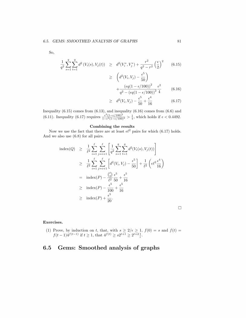
6.5. GEMS: SMOOTHED ANALYSIS OF GRAPHS 81

So,

1

q2

q∑s=1

q∑t=1

d2 (Vi(s), Vj(t)) ≥ d2(V ∗i , V∗j ) +

r2

q2 − r2

( ε2

)2

(6.15)

≥(d2(Vi, Vj)−

ε5

50

)+

(εq(1− ε/100))2

q2 − (εq(1− ε/100))2

ε2

4(6.16)

≥ d2(Vi, Vj)−ε5

50+ε4

16(6.17)

Inequality (6.15) comes from (6.13), and inequality (6.16) comes from (6.6) and

(6.11). Inequality (6.17) requires ε2(1−ε/100)2

1−ε2(1−ε/100)2 >14 , which holds if ε < 0.4492.

Combining the resultsNow we use the fact that there are at least ε`2 pairs for which (6.17) holds.

And we also use (6.8) for all pairs.

index(Q) ≥ 1

`2

∑i=1

∑j=i+1

[1

q2

q∑s=1

q∑t=1

d2(Vi(s), Vj(t))

]

≥ 1

`2

∑i=1

∑j=i+1

[d2(Vi, Vj)−

ε5

50

]+

1

`2

(ε`2

ε4

16

)

= index(P )−(`2

)`2

ε5

50+ε5

16

≥ index(P )− ε5

100+ε5

16

≥ index(P ) +ε5

20.

Exercises.

(1) Prove, by induction on t, that, with s ≥ 2/ε ≥ 1, f(0) = s and f(t) =f(t− 1)4f(t−1) if t ≥ 1, that 4f(t) ≥ s2t+1 ≥ 2t+2 1

ε .

6.5 Gems: Smoothed analysis of graphs


Chapter 7

Properties ofEpsilon-Regular Pairs

There are some interesting properties of regular pairs emerge directly from thedefinition and we leave most of them as an exercise.

Proposition 7.0.1 Let ε′ > ε. If (A,B) is an ε-regular pair, then (A,B) is anε′-regular pair.

Proposition 7.0.2 Let G be graph defined by the pair (A,B) and let G denotethe bipartite complement of G. That is, G is a bipartite graph defined on thepair (A,B) with the property that for any a ∈ A and b ∈ B, then a ∼G b iffa 6∼G b.

If G is ε-regular with density d, then G is ε-regular with density 1− d.

Proposition 7.0.3 Let (A,B) be an ε-regular pair with density d. Let A′ be theset of vertices with deg(a) ∈ [(d− ε)|B|, (d+ ε)|B|]. Then, |A′| ≥ (1− 2ε)|A|.

Exercises.




7.1 The Intersection Property

Proposition 7.1.1 (Intersection Property) Let (A,B) be ε-regular with den-sity d, 0 < ε < d < 1 and t ≥ 1 be an integer. If Y ⊆ B and (d−ε)t−1|Y | ≥ ε|B|,then

#

(a1, a2, . . . , at) ∈ At :

∣∣∣∣∣Y ∩(

t⋂i=1

N(ai)

)∣∣∣∣∣ < (d− ε)t|Y |

≤ tε|A|t.

83

84 CHAPTER 7. PROPERTIES OF EPSILON-REGULAR PAIRS

Proof. This is proven by induction on t. Let t = 1 and X = a ∈ A :|Y ∩N(x)| < (d− ε)|Y |. The fact that (A,B) is ε-regular with density d givesthat |X| < ε|A|, otherwise, since |Y | ≥ ε|B|, d(X,Y ) < (d− ε), a contradictionto the definition of X.

Suppose the statement is true for t− 1.

Let X =

(a1, . . . , at) ∈ At :∣∣∣Y ∩ (⋂ti=1N(ai)

)∣∣∣ < (d− ε)t|Y |

, let X1 =(a1, . . . , at−1) ∈ At :

∣∣∣Y ∩ (⋂t−1i=1 N(ai)

)∣∣∣ < (d− ε)t−1|Y |

.

Let ~x = (a1, . . . , at−1) 6∈ X1 and Y ′ = Y ∩⋂t−1i=1 N(xi). Let X ′ = X ′(~x) =

a ∈ A : |Y ′ ∩ N(x)| < (d − ε)|Y ′|. The fact that (A,B) is ε-regular withdensity d gives that |X ′| < ε|A|, otherwise, since |Y ′| ≥ ε|B|, d(X ′, Y ′) < (d−ε),a contradiction to the definition of X.

By the inductive hypothesis,

|X | ≤ |X1||A|+∑

~x∈X\X1

|X ′(~x)| < (t− 1)ε|A|t−1 · |A|+ |A|t−1 · (ε|A|) = tε|A|t.

A similar proof to that of the Intersection Property gives that there is onlya small number of t-tuples whose common intersection is too large.

Proposition 7.1.2 Let (A,B) be ε-regular with density d, 0 < ε < d < 1 andk ≥ 1 be an integer. If Y ⊆ B and (d+ ε)t−1|Y | ≥ ε|B|, then

#

~a = (a1, a2, . . . , at) ∈ At :

∣∣∣∣∣Y ∩(

t⋂i=1

N(xi)

)∣∣∣∣∣ > (d+ ε)t|Y |

≤ tε|A|t.

One application of the intersection property is that complete bipartite graphsare present in regular pairs.

Corollary 7.1.3 Fix positive integers k, k′. If (A,B) is an ε-regular pair withdensity d, ε d and n = |A| = |B|, then if n is large enough, (A,B) has a copyof Kk,k′

The intersection property can be generalized as well. The condition on thesize of Y could be tightened, but it is unnecessary for applications.

Proposition 7.1.4 (Generalized Intersection Property) Let (A,B) be ε-regular with density d, 0 < ε < d < 1 and k ≥ 1 and ` ∈ 0, 1, . . . , k be integers.If Y ⊆ B and (mind, 1− d − ε)k−1|Y | ≥ ε|B|, then

#

~x ∈ Ak :

∣∣∣∣∣Y ∩(⋂i=1

N(xi)

)∩

(k⋂

i=`+1

N(xi)

)∣∣∣∣∣6∈[(d− ε)`(1− d− ε)k−`|Y |, (d+ ε)`(1− d+ ε)k−`|Y |

] ≤ 2kε|A|k.

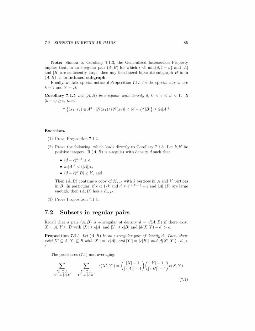
7.2. SUBSETS IN REGULAR PAIRS 85

Note: Similar to Corollary 7.1.3, the Generalized Intersection Propertyimplies that, in an ε-regular pair (A,B) for which ε mind, 1 − d and |A|and |B| are sufficiently large, then any fixed sized bipartite subgraph H is in(A,B) as an induced subgraph.

Finally, we take special notice of Proposition 7.1.1 for the special case wherek = 2 and Y = B:

Corollary 7.1.5 Let (A,B) be ε-regular with density d, 0 < ε < d < 1. If(d− ε) ≥ ε, then

#

(x1, x2) ∈ A2 : |N(x1) ∩N(x2)| < (d− ε)2|B|≤ 2ε|A|2.

Exercises.


(2) Prove the following, which leads directly to Corollary 7.1.3: Let k, k′ bepositive integers. If (A,B) is ε-regular with density d such that

• (d− ε)k−1 ≥ ε.• kε|A|k < (|A|)k,

• (d− ε)k|B| ≥ k′, and

Then (A,B) contains a copy of Kk,k′ with k vertices in A and k′ verticesin B. In particular, if ε < 1/k and d ≥ ε1/(k−1) + ε and |A|, |B| are largeenough, then (A,B) has a Kk,k′ .


7.2 Subsets in regular pairs

Recall that a pair (A,B) is ε-irregular of density d = d(A,B) if there existX ⊆ A, Y ⊆ B with |X| ≥ ε|A| and |Y | ≥ ε|B| and |d(X,Y )− d| > ε.

Proposition 7.2.1 Let (A,B) be an ε-irregular pair of density d. Then, thereexist X ′ ⊆ A, Y ′ ⊆ B with |X ′| = dε|A|e and |Y ′| = dε|B|e and |d(X ′, Y ′)−d| >ε.

The proof uses (7.1) and averaging.∑X′ ⊆ A

|X′| = dε|A|e

∑Y ′ ⊆ A

|Y ′| = dε|B|e

e(X ′, Y ′) =

(|X| − 1

dε|A|e − 1

)(|Y | − 1

dε|B|e − 1

)e(X,Y )

(7.1)

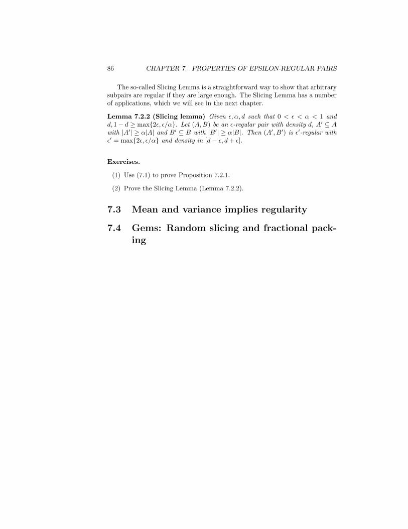
86 CHAPTER 7. PROPERTIES OF EPSILON-REGULAR PAIRS

The so-called Slicing Lemma is a straightforward way to show that arbitrarysubpairs are regular if they are large enough. The Slicing Lemma has a numberof applications, which we will see in the next chapter.

Lemma 7.2.2 (Slicing lemma) Given ε, α, d such that 0 < ε < α < 1 andd, 1− d ≥ max2ε, ε/α. Let (A,B) be an ε-regular pair with density d, A′ ⊆ Awith |A′| ≥ α|A| and B′ ⊆ B with |B′| ≥ α|B|. Then (A′, B′) is ε′-regular withε′ = max2ε, ε/α and density in [d− ε, d+ ε].

Exercises.

(1) Use (7.1) to prove Proposition 7.2.1.

(2) Prove the Slicing Lemma (Lemma 7.2.2).

7.3 Mean and variance implies regularity

7.4 Gems: Random slicing and fractional pack-ing

Chapter 8

Subgraph Applications ofthe Regularity Lemma

For many of these applications, we will be investigating a number of propertiesof large graphs. As such, the notation Gn denotes a graph G on n vertices.

There is some important notation that comes into play when the regularitylemma is used:

Definition 8.0.1 We say that ε is small enough relative to δ and write ε δif there is a function f of δ such that ε < f(δ).

The “” notation is used for parameters in many theorems that use the regu-larity lemma.

8.1 Erdos-Stone-Simonovits

Theorem 8.1.1 is due to Erdos and Stone in 1946. It was generalized by Erdosand Simonovits (Theorem 8.1.2) in 1966 and is, hence, usually called Erdos-Stone-Simonovits. The theorem predates Szemeredi’s regularity lemma and didnot use it. A proof of Erdos-Stone that does not use the regularity lemma canbe found in Combinatorial Geometry by Pach and Agarwal [PA95].1

For integers p ≥ 2 and t ≥ 1, we use Kp(t) to denote the complete p-partitegraph with t vertices in each partite set.

Theorem 8.1.1 (Erdos-Stone, [ES46]) Let p ≥ 2 and t ≥ 1 be integers andlet ε > 0. There exists an n0 = n0(p, t, ε) such that if a graph G has at least

n ≥ n0 vertices and e(G) ≥(

1− 1p−1 + ε

)n2

0

2 , then there exists a copy of Kp(t)

in G.

1Is it true?

87

88CHAPTER 8. SUBGRAPH APPLICATIONS OF THE REGULARITY LEMMA

In the case of t = 1, this is nothing more than an immediate consequence ofTuran’s theorem (Theorem 3.3.1):

e(Gn) ≥(

1− 1

p− 1

)n2

2⇒ Gn ⊇ Kp.

For a family of graphs F , we use the extremal notation ex(n,F) to denotethe maximum number of edges in a graph Gn that has no F ∈ F as a subgraph.

Theorem 8.1.2 (Erdos-Simonovits, [ES66]) Let F be a family of graphssuch that minχ(F ) : F ∈ F = p > 2

ex(n,F) =

(1− 1

p− 1

)n2

2+ o(n2).

For our proof of Erdos-Stone, we will use Lemma 8.1.3, a statement whichwill be following will be generalized later by the Key Lemma, but it is worthinvestigating it in detail so as to see how Szemeredi’s regularity lemma is appliedin these contexts.

Lemma 8.1.3 Let p ≥ 2 and t ≥ 1 be integers. Then, for all d ∈ (0, 1),there exist ε0 = ε0(d, t, p), and L0 = L0(d, t, p) such that whenever ε ≤ ε0 and(V1, . . . , Vp) is a p-tuple that is pairwise ε-regular with density at least d and|V1| = . . . = |Vp| = L ≥ L0, it contains a copy of Kp(t).

I.e., if ε d and L is large enough, then a copy of Kp(t) is present in abalanced p-tuple with enough vertices in each part that pairwise is ε-regular withdensity at least d contains a copy

Proof. We will proceed by induction on p. For the base case of p = 2, wehave a pair which is ε-regular with density d ε, so we just use the intersectionproperty (Proposition 7.1.1). Here we need (d − ε)t−1L ≥ εL, (d − ε)tL ≥ tand tεLt < Lt in order to force a copy of Kt,t = K2(t). Choosing ε0(d, t, 2) =min(d/2)t, 1/t and L0(d, t, 2) = t/(d/2)t suffices

Now, suppose the statement is true for p ≥ 2, we have ε0 = ε0(d, t, p) andL0 = L0(d, t, p), so we need to prove it for p + 1, and obtain ε0(d, t, p + 1) andL0(d, t, p+ 1).

Again, we use the intersection property. If (d − ε)t−1L ≥ εL then we canapply the intersection property to every pair (Vi, Vp+1) for i = 1, . . . , p. Conse-quently,

#

~a ∈ V tp+1 :

∣∣∣∣∣t⋂i=1

N(ai)

∣∣∣∣∣ ≤ (d− ε)tL for any Vi with 1 ≤ i ≤ p

≤ tpεLt.

If tpε < 1, ∃ t vertices with neighborhoods of size at least (d − ε)tL in each ofV1, . . . , Vp.

8.1. ERDOS-STONE-SIMONOVITS 89

Let V ′i ⊆ Vi, with |V ′i | ≥ d(d− ε)tLe. As long as d(d− ε)tLe ≥ εL, for i 6= j,

the pair (V ′i , V′j ) is max

2ε, ε

(d−ε)t

-regular of density greater than (d− ε).

We need (d− ε)t ≥ ε. If 2ε < ε0(d− ε, t, p) andε

(d− ε)t< ε0(d− ε, t, p) and

(d − ε)t < L0(d − ε, t, p), then we can apply the inductive hypothesis, and seethat (V ′1 , . . . , V

′p) contains Kp(t), giving a copy of Kp+1(t) in the original graph.

Summarizing the requirements for ε0 and L0, ensure that

ε0(d, t, p+ 1) ≤ min

1/2, (d− ε)t· ε0(d, t, p)

and

L0(d, t, p+ 1) ≤ 1

(d− ε)tL0(d− ε, t, p).

Setting ε0(d, t, p) = min(d/p)t, 1/((p− 1)t) and L0(d, t, p) = t/(d/p)t suffices.

It takes a good deal of work to determine values of ε0 and L0 to make surethat the theorem works, but if we simply say that ε d and L is large enough,then the existence of Kp(t) is guaranteed.

Now we return to Erdos-Stone:

Proof of Theorem 8.1.1. We construct a graph on the clusters V1, . . . , V`of the Szemeredi partition of Gn. This is a common technique and this graphis called variously the cluster graph, reduced graph or Szemeredi graph.For this proof, we will denote it as GSz. The literature sometimes refers to thisgraph as Gr.

Apply Szemeredi’s regularity lemma to G with ε′ (which we will choose later)and m =

⌈(ε′)−1

⌉. For some d ∈ (0, 1) (again, chosen later) and Szemeredi

partition V0 + V1 + · · · + V`, define GSz on the vertex set v1, . . . , v` such thatvi ∼ vj if and only if the pair (Vi, Vj) is ε-regular with density at least d.

First, we will create G′n by deleting edges from Gn that are (1) incident toV0, (2) in an irregular pair or (3) inside a cluster. The number of such edges isat most

(1) ε′n · n ≤ ε′n2

(2) ε′`2 · L2 ≤ ε′n2

(3) `(L2

)≤ (`L)2

2` ≤n2

2m ≤ ε′n2/2.

Consequently the total amount of such edges is less than 3ε′n2.

Now, we count the number of edges in GSz.

e(G)− 3ε′n2 ≤ e(G′n) ≤(`

2

)dL2 + e(GSz)(L2−dL2) ≤ d

2n2 + e(GSz)(1−d)L2.


Consequently,

e(GSz) ≥ e(G)− (3ε′ + d/2)n2

(1− d)L2

≥ (1− 1/(p− 1) + ε)(n2/2)− (3ε′ + d/2)

(1− d)L2

≥(

1− 1

p− 1

)n2

2+

(ε

2− 3ε′ − d

2

)`2.

So, if 3ε′+d/2 < ε, then we can apply Turan’s theorem to GSz, which impliesGSz has a p-clique. We can apply Lemma 8.1.3 to the clusters that correspondto this clique, which yields the copy of Kp(t).

8.2 Degree form and number of copies of a graph

Szemeredi’s regularity lemma has a number of different forms, the most usefulfor embedding problems is

Theorem 8.2.1 (Regularity lemma, degree form) For every ε > 0, thereis an M = M(ε) such that if G = (V,E) is any graph on n vertices and d ∈ [0, 1]is any real number, then there is a partition of the vertex set V into `+1 clustersV0 + V1 + · · ·+ V` and there is a subgraph G′ ⊆ G such that

• ` ≤M

• |V0| < εn

• |V1| = |V2| = · · · = |V`| ≤ εn

• degG′(v) > degG(v)− (d+ ε)n

• e(G′[Vi]) = 0

• ALL pairs of clusters are ε-regular with density either 0 or at least d.

We leave the proof of Theorem 8.2.1 to the exercises, but note that, like theoriginal form (Theorem 6.3.1), this theorem will refine an existing equipartition.For example, if G is bipartite, we may assume that each of the clusters V1, . . . , V`spans only one partite set. Only the leftover set V0 will span multiple partitesets.

8.2.2 Number of copies of a graph

The survey KS96 gives a number of immediate and insightful applications ofthe degree form. We use ‖H → Gn‖ to denote the number of embeddings of Hin Gn. I.e., the number of copies of H in Gn.

8.2. DEGREE FORM AND NUMBER OF COPIES OF A GRAPH 91

Theorem 8.2.3 (Number of copies of H) Let H be a graph with h verticesand chromatic number p. Let β < 0 and ε = (β/6)h. If n is large enough and

e(Gn) ≥(

1− 1p−1 + β

)n2

2 , then ‖H → Gn‖ ≥(

εnM(ε)

)h, where M(ε) is given

by Theorem 8.2.1.

The proof of Theorem 8.2.3 is left as an exercise, given the following KeyLemma:

Lemma 8.2.4 (Key Lemma) Let d > ε ≥ 0. Given a graph R and a positiveinteger t, the graph R(t) is constructed by replacing each vertex of R by t verticesand each edge by Kt,t (nonedges are replaced with empty bipartite graphs). Givena graph R and a positive integer L, construct G by replacing each vertex of Rby L vertices and each edge with ε-regular pairs of density at least d. Let Hbe a subgraph of R(t), h = |V (H)| and maximum degree ∆ = ∆(H) > 0. Let

δ = d− ε and ε0 = δ∆

∆+2 . If ε < ε0 and t− 1 ≤ ε0L, then

‖H → G‖ > (ε0L)h.

Proof. We will prove the following statement and leave it to the reader toconclude that it implies the statement of the Key Lemma.

If t− 1 ≤ (δ∆ −∆ε)L, then ‖H → G‖ >((δ∆ −∆ε)L− (t− 1)

)h.

Define V (H) = v1, . . . , vh and assign each vi to a cluster according to someembedding of H in R(t). We will choose v1, v2, . . . , vh in sequence. At stagei ≥ 1, we denote Ci,j to be the subset of the cluster of vertices that are eligibleto be chosen for vj , given that v1, . . . , vi have already been chosen. Hence,C0,j ⊇ C1,j ⊇ · · · ⊇ Cj−1,j .

At stage i ≥ 1, we do two things:

(1) Choose vi ∈ Ci−1,i such that degCi−1,j(vi) ≥ δ|Ci−1,j | for all j > i with

vj ∼H vi.

(2) Update Ci,jdef= Ci−1,j ∩N(vi) for all j > i with vj ∼H vi.

For j > i, let di,j = |k ∈ 1, . . . , i : vk ∼H vj|. So, |Ci,j | ≥ δdi,jL. Con-sequently, |Ci,j | ≥ δdi,jL ≥ δ∆L > εL. So, throughout this process, every C setis larger than εL. To see that the process completes with an embedding of H,vi can be chosen because of the ε-regularity of the clusters. If S ⊂ Ci−1,i is theset of vertices with fewer than δ|Ci−1,j | neighbors in Ci−1,j , then the density isless than δ = d− ε, implying |S| < εL. There are at most ∆ such pairs for anyi.

As a result, there are at most ∆εL + (t − 1) vertices in Ci−1,i that vicannot be assigned to. The t − 1 accounts for the fact that vi cannot beany of v1, . . . , vi−1, which might have come from the same cluster. There-fore, we have

(δ∆ −∆ε

)L − (t − 1) choices for vi. Consequently, there are(

(δ∆ −∆ε)L− (t− 1))h

embeddings.


One thing that makes Theorem 8.2.3 so striking is that, trivially, ‖H →Gn‖ ≤ nh, but there is a Gn with minimum degree

(1− 1

p−1 − o(1))n2

2 , namely

the Turan graph, that has no copies of H. But if the minimum degree is in-creased slightly, the number of embeddings is within a constant of the maximumpossible.

Another striking observation, the details of which we leave to the reader, isin some ways, the contrapositive of Theorem 8.2.3. It says that we can choosea small set of edges to cover all copies of H, even if the number of such copiesis proportional to nh.

Theorem 8.2.5 (Covering copies of H by edges) For every β > 0 and Ha graph on h vertices, there exists γ = γ(β,H) > 0 such that if ‖H → Gn‖ ≤γnh, then by deleting at most βn2 edges, Gn can be made H-free.

Exercises.

(1) Prove the degree form of the Regularity Lemma from the original state-ment. Hint: Apply Theorem 6.3.1 with parameters ε = ε2DF and m =dεDFe. Follow the proof of Theorem 8.1.1.

(2) Prove Theorem 8.2.3 using the Key Lemma, Lemma 8.2.4. Hint: Followthe proof of Theorem 8.1.1.

8.3 Blow-up lemma

8.3.1 Alon-Yuster

8.3.2 Embedding theorems

8.3.3 Zhao’s theorem on bipartite tiling

8.3.4 Tripartite version of Hajnal-Szemeredi

Chapter 9

Induced SubgraphApplications of theRegularity Lemma

9.1 An important parameter

9.2 Generalized intersection property

9.3 Number of graphs of a certain type

9.4 Probability that a graph is in a hereditaryproperty

9.5 Edit distance

93

94CHAPTER 9. INDUCED SUBGRAPH APPLICATIONS OF THE REGULARITY LEMMA

9.6 Expander graphs

Bibliography

[AK97] Noga Alon and Michael Krivelevich, The concentration of the chro-matic number of random graphs, Combinatorica 17 (1997), no. 3,303–313. MR MR1606020 (98m:05173)

[AKS80] Miklos Ajtai, Janos Komlos, and Endre Szemeredi, A note on Ram-sey numbers, J. Combin. Theory Ser. A 29 (1980), no. 3, 354–360.MR MR600598 (82a:05064)

[AKS81] , A dense infinite Sidon sequence, European J. Combin. 2(1981), no. 1, 1–11. MR MR611925 (83f:10056)

[AS00] Noga Alon and Joel Spencer, The probabilistic method, second ed.,Wiley-Interscience Series in Discrete Mathematics and Optimiza-tion, Wiley-Interscience [John Wiley & Sons], New York, 2000, Withan appendix on the life and work of Paul Erdos. MR MR1885388(2003f:60003)

[Ber08] Felix Bernstein, Zur theorie der trigonometrische reihen, Leipz. Ber60 (1908), 325–328.

[BF92] Laszlo Babai and Peter Frankl, Linear algebra methods in combina-torics with applications to geometry and computer science, Univer-sity of Chicago Department of Computer Science, Chicago, IL, 1992,(Preliminary Version 2).

[Bir46] Garrett Birkhoff, Three observations on linear algebra, Univ. Nac.Tucuman. Revista A. 5 (1946), 147–151. MR MR0020547 (8,561a)

[Bol88] Bela Bollobas, The chromatic number of random graphs, Combina-torica 8 (1988), no. 1, 49–55. MR MR951992 (89i:05244)

[Bol98] , Modern graph theory, Graduate Texts in Mathematics, vol.184, Springer-Verlag, New York, 1998. MR MR1633290 (99h:05001)

[Bol01] , Random graphs, second ed., Cambridge Studies in Ad-vanced Mathematics, vol. 73, Cambridge University Press, Cam-bridge, 2001. MR MR1864966 (2002j:05132)

95

96 BIBLIOGRAPHY

[Bou59] V.Y. Bouniakowsky, Sur quelques inegalites concernant les integralesaux differences finies, Mem. Acad. Sci. St. Petersbourg I (1859),no. 9, 1–18.

[CAH63] Keresztely Corradi and A. Andras Hajnal, On the maximal numberof independent circuits in a graph, Acta Math. Acad. Sci. Hungar.14 (1963), 423–439. MR MR0200185 (34 #84)

[Cam99] Peter J. Cameron, Permutation groups, London Mathematical Soci-ety Student Texts, vol. 45, Cambridge University Press, Cambridge,1999. MR MR1721031 (2001c:20008)

[Cau21] Augustin-Louis Cauchy, Oeuvres 2, vol. III, 1821.

[CGFS86] Fan R.K. Chung, Ronald L. Graham, Peter Frankl, and James B.Shearer, Some intersection theorems for ordered sets and graphs, J.Combin. Theory Ser. A 43 (1986), no. 1, 23–37. MR MR859293(87k:05002)

[Dil50] Robert P. Dilworth, A decomposition theorem for partially or-dered sets, Ann. of Math. (2) 51 (1950), 161–166. MR MR0032578(11,309f)

[Dir52] Gabriel A. Dirac, Some theorems on abstract graphs, Proc. LondonMath. Soc. (3) 2 (1952), 69–81. MR MR0047308 (13,856e)

[EFS56] Peter Elias, Amiel Feinstein, and Claude E. Shannon, A note on themaximum flow through a network, IRE Transactions on InformationTheory 2 (1956), no. 4, 117–119.

[Ege31] Eugene (Jeno) Egervary, On combinatorial properties of matrices,Mat. Lapok 38 (1931), 16–28, (Hungarian with German summary).

[EH89] Pal Erdos and Andras Hajnal, Ramsey-type theorems, Discrete Appl.Math. 25 (1989), no. 1-2, 37–52, Combinatorics and complexity(Chicago, IL, 1987). MR MR1031262 (90m:05091)

[EHR65] Pal Erdos, Andras Hajnal, and Richard Rado, Partition relations forcardinal numbers, Acta Math. Acad. Sci. Hungar. 16 (1965), 93–196.MR MR0202613 (34 #2475)

[EL75] Pal Erdos and Laszlo Lovasz, Problems and results on 3-chromatichypergraphs and some related questions, Infinite and finite sets (Col-loq., Keszthely, 1973; dedicated to P. Erdos on his 60th birth-day), Vol. II, North-Holland, Amsterdam, 1975, pp. 609–627. Colloq.Math. Soc. Janos Bolyai, Vol. 10. MR MR0382050 (52 #2938)

[ER52] Pal Erdos and Richard Rado, Combinatorial theorems on classifica-tions of subsets of a given set, Proc. London Math. Soc. (3) 2 (1952),417–439. MR MR0065615 (16,455d)

BIBLIOGRAPHY 97

[ER60] Pal Erdos and Alfred Renyi, On the evolution of random graphs,Magyar Tud. Akad. Mat. Kutato Int. Kozl. 5 (1960), 17–61. MRMR0125031 (23 #A2338)

[Erd47] Pal Erdos, Some remarks on the theory of graphs, Bull. Amer. Math.Soc. 53 (1947), 292–294. MR MR0019911 (8,479d)

[Erd59] Pal Erdos, Graph theory and probability, Canad. J. Math. 11 (1959),34–38. MR MR0102081 (21 #876)

[Erd61] , Graph theory and probability. II, Canad. J. Math. 13 (1961),346–352. MR MR0120168 (22 #10925)

[Erd70] , On the graph theorem of Turan, Mat. Lapok 21 (1970),249–251 (1971). MR MR0307975 (46 #7090)

[ES46] Pal Erdos and Arthur H. Stone, On the structure of linear graphs,Bull. Amer. Math. Soc. 52 (1946), 1087–1091. MR MR0018807(8,333b)

[ES66] Pal Erdos and Miklos Simonovits, A limit theorem in graph the-ory, Studia Sci. Math. Hungar 1 (1966), 51–57. MR MR0205876 (34#5702)

[ES72] Pal Erdos and Endre Szemeredi, On a Ramsey type theorem, Period.Math. Hungar. 2 (1972), 295–299, Collection of articles dedicated tothe memory of Alfred Renyi, I. MR MR0325446 (48 #3793)

[FF56] Lester R. Ford Jr. and Delbert R. Fulkerson, Maximal flow througha network, Canad. J. Math. 8 (1956), 399–404. MR MR0079251(18,56h)

[Fro17] Georg Frobenius, Uber zerlegbare Determinanten, Sitzungsber.Konig. Preuss. Adad. Wiss. XVIII (1917), 274–277.

[GT04] David Galvin and Prasad Tetali, On weighted graph homomor-phisms, Graphs, morphisms and statistical physics, DIMACS Ser.Discrete Math. Theoret. Comput. Sci., vol. 63, Amer. Math. Soc.,Providence, RI, 2004, pp. 97–104. MR 2056231 (2005c:05015)

[GY68] Jack E. Graver and James Yackel, Some graph theoretic results as-sociated with Ramsey’s theorem, J. Combinatorial Theory 4 (1968),125–175. MR MR0225685 (37 #1278)

[Haf03] Paul R. Hafner, The Hoffman-Singleton graph and its auto-morphisms, J. Algebraic Combin. 18 (2003), no. 1, 7–12. MRMR2002216 (2004f:05078)

[Hal35] Philip Hall, On representation of subsets, J. London Math. Soc. 10(1935), 26–30.

98 BIBLIOGRAPHY

[HHMS10] H. Tracy Hall, Leslie Hogben, Ryan Martin, and Bryan Shader, Ex-pected values of parameters associated with the minimum rank of agraph, Linear Algebra Appl. (2010), 17pp., to appear.

[HHPa] Hatos-Hall Productions, The Monty Hall problem,http://www.letsmakeadeal.com/problem.htm, accessed 18February, 2008.

[HHPb] , The official Let’s Make A Deal website,http://www.letsmakeadeal.com/, accessed 18 February, 2008.

[HS60] Alan J. Hoffman and Robert R. Singleton, On Moore graphs withdiameters 2 and 3, IBM J. Res. Develop. 4 (1960), 497–504. MRMR0140437 (25 #3857)

[HS70] Andras Hajnal and Endre Szemeredi, Proof of a conjecture of P.Erdos, Combinatorial theory and its applications, II (Proc. Colloq.,Balatonfured, 1969), North-Holland, Amsterdam, 1970, pp. 601–623. MR MR0297607 (45 #6661)

[HW73] Carl Hierholzer and Christian Wiener, Ueber die Moglichkeit, einenLinenzug ohne Wiederholung und ohne Unterbrechung zu umfahren,Math. Ann. 6 (1873), no. 1, 30–32. MR MR1509807

[J LR00] Svante Janson, Tomasz Luczak, and Andrej Rucinski, Randomgraphs, Wiley-Interscience Series in Discrete Mathematics and Op-timization, Wiley-Interscience, New York, 2000. MR MR1782847(2001k:05180)

[Kah01] Jeff Kahn, An entropy approach to the hard-core model on bipartitegraphs, Combin. Probab. Comput. 10 (2001), no. 3, 219–237. MR1841642 (2003a:05111)

[Kim95] Jeong Han Kim, The Ramsey number R(3, t) has order of magnitudet2/ log t, Random Structures Algorithms 7 (1995), no. 3, 173–207.MR MR1369063 (96m:05140)

[KK08] Hal A. Kierstead and Alexandr V. Kostochka, A short proof of theHajnal-Szemeredi theorem on equitable colouring, Combin. Probab.Comput. 17 (2008), no. 2, 265–270. MR MR2396352 (2009a:05071)

[Kon31] Denes Konig, Graphen und Matrizen, Mat. Lapok 38 (1931), 116–119.

[KS96] Janos Komlos and Miklos Simonovits, Szemeredi’s regularity lemmaand its applications in graph theory, Combinatorics, Paul Erdosis eighty, Vol. 2 (Keszthely, 1993), Bolyai Soc. Math. Stud.,vol. 2, Janos Bolyai Math. Soc., Budapest, 1996, pp. 295–352. MRMR1395865 (97d:05172)

BIBLIOGRAPHY 99

[KSSS02] Janos Komlos, Ali Shokoufandeh, Miklos Simonovits, and EndreSzemeredi, The regularity lemma and its applications in graph the-ory, Theoretical aspects of computer science (Tehran, 2000), LectureNotes in Comput. Sci., vol. 2292, Springer, Berlin, 2002, pp. 84–112.MR MR1966181 (2004d:05106)

[Lef87] Hanno Lefmann, A note on Ramsey numbers, Studia Sci. Math.Hungar. 22 (1987), no. 1-4, 445–446. MR MR932230 (89d:05132)

[Lov75] Laszlo Lovasz, Three short proofs in graph theory, J. CombinatorialTheory Ser. B 19 (1975), no. 3, 269–271. MR MR0396344 (53 #211)

[LR93] Hanno Lefmann and Vojtech Rodl, On canonical Ramsey numbersfor coloring three-element sets, Finite and infinite combinatorics insets and logic (Banff, AB, 1991), NATO Adv. Sci. Inst. Ser. C Math.Phys. Sci., vol. 411, Kluwer Acad. Publ., Dordrecht, 1993, pp. 237–247. MR MR1261209 (94k:05211)

[LR95] , On Erdos-Rado numbers, Combinatorica 15 (1995), no. 1,85–104. MR MR1325273 (96a:05003)

[ Luc91] Tomasz Luczak, A note on the sharp concentration of the chromaticnumber of random graphs, Combinatorica 11 (1991), no. 3, 295–297.MR MR1122014 (92k:05118)

[McD89] Colin McDiarmid, On the method of bounded differences, Surveysin combinatorics, 1989 (Norwich, 1989), London Math. Soc. Lec-ture Note Ser., vol. 141, Cambridge Univ. Press, Cambridge, 1989,pp. 148–188. MR MR1036755 (91e:05077)

[Men27] Karl Menger, Zur allgemeinen kurventheorie, Fund. Math. 10(1927), 95–115.

[Mos04] Ivan Moscovich, The Monty Hall problem & other puzzles, Sterling,2004.

[MS] Martin Macaj and Jozef Siran, Search for properties of the missingMoore graph, Linear Algebra and its Applications, To appear.

[Ore60] Oystein Ore, Note on Hamilton circuits, Amer. Math. Monthly 67(1960), 55. MR MR0118683 (22 #9454)

[PA95] Janos Pach and Pankaj K. Agarwal, Combinatorial geometry, Wiley-Interscience Series in Discrete Mathematics and Optimization, JohnWiley & Sons Inc., New York, 1995, A Wiley-Interscience Publica-tion. MR MR1354145 (96j:52001)

[Rad94] Stanis law P. Radziszowski, Small Ramsey numbers, Electron. J.Combin. 1 (1994), Dynamic Survey 1, 30 pp. (electronic), accessed28 Jan 2010. MR MR1670625 (99k:05117)

100 BIBLIOGRAPHY

[Rad01] Jaikumar Radhakrishnan, Entropy and counting, IIT Kharagpur,Golden Jubilee Volume on Computational Mathematics, Modellingand Algorithms (J.C. Mishra, ed.), Narosa Publishers, New Delhi,2001.

[Ram30] Frank P. Ramsey, On a problem of formal logic, Proc. Lond. Math.Soc. 30 (1930), 264–286.

[Sch88] H. A. Schwarz, Ueber ein Flachen kleinsten Flacheninhalts betref-fendes Problem der Variationsrechnung, Acta Societatis scientarumFennicae XV (1888), 316–362.

[She83] James B. Shearer, A note on the independence number of triangle-free graphs, Discrete Math. 46 (1983), no. 1, 83–87. MR MR708165(85b:05158)

[She91] , A note on the independence number of triangle-free graphs.II, J. Combin. Theory Ser. B 53 (1991), no. 2, 300–307. MRMR1129557 (92k:05073)

[Sin68] Robert R. Singleton, There is no irregular Moore graph, Amer.Math. Monthly 75 (1968), 42–43. MR MR0225679 (37 #1272)

[Spe78] Joel Spencer, Asymptotic lower bounds for Ramsey functions, Dis-crete Math. 20 (1977/78), no. 1, 69–76. MR MR0491337 (58#10600)

[SS87] Eli Shamir and Joel Spencer, Sharp concentration of the chromaticnumber on random graphs Gn,p, Combinatorica 7 (1987), no. 1, 121–129. MR MR905159 (88i:05164)

[Sze75] Endre Szemeredi, On sets of integers containing no k elements inarithmetic progression, Acta Arith. 27 (1975), 199–245, Collectionof articles in memory of Juriı Vladimirovic Linnik. MR MR0369312(51 #5547)

[Sze78] , Regular partitions of graphs, Problemes combinatoires ettheorie des graphes (Colloq. Internat. CNRS, Univ. Orsay, Or-say, 1976), Colloq. Internat. CNRS, vol. 260, CNRS, Paris, 1978,pp. 399–401. MR MR540024 (81i:05095)

[Tur41] Pal Turan, Eine Extremalaufgabe aus der Graphentheorie, Mat. Fiz.Lapok 48 (1941), 436–452. MR MR0018405 (8,284j)

[Tut47] William T. Tutte, The factorization of linear graphs, J. LondonMath. Soc. 22 (1947), 107–111. MR MR0023048 (9,297d)

[vdW27] Bartel L. van der Waerden, Beweis einer baudetschen vermutung,Nieuw Arch. Wiskunde 15 (1927), 212–216.

BIBLIOGRAPHY 101

[vN53] John von Neumann, A certain zero-sum two-person game equivalentto the optimal assignment problem, Contributions to the theory ofgames, vol. 2, Annals of Mathematics Studies, no. 28, PrincetonUniversity Press, Princeton, N. J., 1953, pp. 5–12. MR MR0054920(14,998i)

[vS97] Marilyn vos Savant, The power of logical thinking, St. Martin’s Grif-fin, New York, 1997.

[Vu10] Van Vu, Chernoff bound, electronic, February 2010, accessed 13February 2010.

[Wei] Eric W. Weisstein, Stirling’s approximation,http://mathworld.wolfram.com/StirlingsApproximation.html,accessed 27 Jan 2008.

[Wil86] Robin J. Wilson, An Eulerian trail through Konigsberg, J. GraphTheory 10 (1986), no. 3, 265–275. MR MR856115 (88a:01015)

[Zha] Yufei Zhao, The number of independent sets in a regular graph,preprint.

Documents

Notes on Extremal Graph Theory - Index of