Embed Size (px)
Citation preview
Extremal questions in graph theory
vorgelegt vonMaya Jakobine Stein
Habilitationschriftdes Fachbereichs Mathematik
der Universitat Hamburg
Hamburg 2009

Contents
1 Introduction 1
2 The Loebl–Komlos–Sos conjecture 5
2.1 History of the conjecture . . . . . . . . . . . . . . . . . . . . . 5
2.2 Special cases of the Loebl–Komlos–Sos conjecture . . . . . . . 6
2.3 The regularity approach . . . . . . . . . . . . . . . . . . . . . 6
2.4 Discussion of the bounds . . . . . . . . . . . . . . . . . . . . . 7
3 An approximate version of the LKS conjecture 9
3.1 An approximate version and an extension . . . . . . . . . . . . 9
3.2 Preliminaries . . . . . . . . . . . . . . . . . . . . . . . . . . . 10
3.2.1 Regularity . . . . . . . . . . . . . . . . . . . . . . . . . 10
3.2.2 The matching . . . . . . . . . . . . . . . . . . . . . . . 13
3.3 Proof of Theorem 2.3.3 . . . . . . . . . . . . . . . . . . . . . . 15
3.3.1 Overview . . . . . . . . . . . . . . . . . . . . . . . . . 15
3.3.2 Preparations . . . . . . . . . . . . . . . . . . . . . . . . 18
3.3.3 Partitioning the tree . . . . . . . . . . . . . . . . . . . 20
3.3.4 The switching . . . . . . . . . . . . . . . . . . . . . . . 23
3.3.5 Partitioning the matching . . . . . . . . . . . . . . . . 25
3.3.6 Embedding lemmas for trees . . . . . . . . . . . . . . . 28
3.3.7 The embedding in Case 1 . . . . . . . . . . . . . . . . 33
3.3.8 The embedding in Case 2 . . . . . . . . . . . . . . . . 34
3.4 Proof of Theorem 3.1.1 . . . . . . . . . . . . . . . . . . . . . . 36
4 Solution of the LKS conjecture for special classes of trees 39
4.1 Trees of small diameter and caterpillars . . . . . . . . . . . . . 39
4.2 Proof of Theorem 4.1.1 . . . . . . . . . . . . . . . . . . . . . . 40
4.3 Proof of Theorem 4.1.2 . . . . . . . . . . . . . . . . . . . . . . 45
5 An application of the LKS conjecture in Ramsey Theory 49
5.1 Ramsey numbers . . . . . . . . . . . . . . . . . . . . . . . . . 49
5.2 Ramsey numbers of trees . . . . . . . . . . . . . . . . . . . . . 50
5.3 Proof of Proposition 5.2.2 . . . . . . . . . . . . . . . . . . . . 51
6 t-perfect graphs 53
6.1 An introduction to t-perfect graphs . . . . . . . . . . . . . . . 53
6.2 The polytopes SSP and TSTAB . . . . . . . . . . . . . . . . . 55
6.3 t-perfect line graphs . . . . . . . . . . . . . . . . . . . . . . . . 56
6.4 Squares of cycles . . . . . . . . . . . . . . . . . . . . . . . . . 59
6.5 The main lemma . . . . . . . . . . . . . . . . . . . . . . . . . 60
6.6 Colouring claw-free t-perfect graphs . . . . . . . . . . . . . . . 63
6.7 Characterising claw-free t-perfect graphs . . . . . . . . . . . . 66
6.8 C27 and C2
10 are minimally t-imperfect . . . . . . . . . . . . . 70
7 Strongly t-perfect graphs 75
7.1 Strong t-perfection . . . . . . . . . . . . . . . . . . . . . . . . 75
7.2 Strong t-perfection and t-minors . . . . . . . . . . . . . . . . . 76
7.3 Strongly t-perfect and claw-free . . . . . . . . . . . . . . . . . 78
7.4 Minimally strongly t-imperfect . . . . . . . . . . . . . . . . . . 85
8 Infinite extremal graph theory 89
8.1 An introduction to infinite extremal graph theory . . . . . . . 89
8.2 Terminology for infinite graphs . . . . . . . . . . . . . . . . . 91
8.3 Grid minors . . . . . . . . . . . . . . . . . . . . . . . . . . . . 92
8.4 Connectivity of vertex-transitive graphs . . . . . . . . . . . . . 95
9 Highly connected subgraphs of infinite graphs 97
9.1 The results . . . . . . . . . . . . . . . . . . . . . . . . . . . . 97
9.2 End degrees and more terminology . . . . . . . . . . . . . . . 99
9.3 Forcing highly edge-connected subgraphs . . . . . . . . . . . . 99
9.4 High edge-degree but no highly connected subgraphs . . . . . 104
9.5 Forcing highly connected subgraphs . . . . . . . . . . . . . . . 107
9.6 Linear degree bounds are not enough . . . . . . . . . . . . . . 112
10 Large complete minors in infinite graphs 117
10.1 An outline of this chapter . . . . . . . . . . . . . . . . . . . . 117
10.2 Large complete minors in rayless graphs . . . . . . . . . . . . 118
10.3 Two counterexamples . . . . . . . . . . . . . . . . . . . . . . . 118
10.4 Large relative degree forces large complete minors . . . . . . . 120
10.5 Using large girth . . . . . . . . . . . . . . . . . . . . . . . . . 123
11 Minimal k-(edge)-connectivity in infinite graphs 125
11.1 Four notions of minimality . . . . . . . . . . . . . . . . . . . . 125
11.2 The situation in finite graphs . . . . . . . . . . . . . . . . . . 126
11.3 The situation in infinite graphs . . . . . . . . . . . . . . . . . 128
11.4 Vertex-minimally k-connected graphs . . . . . . . . . . . . . . 132
11.5 Edge-minimally k-edge-connected graphs . . . . . . . . . . . . 135
11.6 Vertex-minimally k-edge-connected graphs . . . . . . . . . . . 137
12 Duality of ends 141
12.1 Duality of graphs . . . . . . . . . . . . . . . . . . . . . . . . . 141
12.2 The cycle space of an infinite graph . . . . . . . . . . . . . . . 143
12.3 Duality for infinite graphs . . . . . . . . . . . . . . . . . . . . 145
12.4 Discussion of our results . . . . . . . . . . . . . . . . . . . . . 145
12.5 ∗ induces a homeomorphism on the ends . . . . . . . . . . . . 148
12.6 Tutte-connectivity . . . . . . . . . . . . . . . . . . . . . . . . 150
12.7 The dual preserves the end degrees . . . . . . . . . . . . . . . 155
vi
Chapter 1
Introduction
Extremal graph theory is a branch of graph theory that seeks to explore theproperties of graphs that are in some way extreme. The classical extremalgraph theoretic theorem and a good example is Turan’s theorem. This theo-rem reveals not only the edge-density but also the structure of those graphsthat are ‘extremal’ without a complete subgraph of some fixed size, whereextremal means that upon the addition of any edge the forbidden subgraphwill appear. This is the type of question we study in extremal graph the-ory, for finite as well as for infinite graphs. In general one asks whethersome invariant – which instead of the edge-density might be the minimumdegree, or the chromatic number, etc – has an influence on the appearanceof substructures, or on another graph invariant.
A typical example of modern extremal graph theory is the Loebl–Komlos–Sos conjecture (LKS-conjecture for short) from 1992. This conjecture isabout whether the existence of subtrees in a graph can be forced by as-suming a large median degree. More precisely, the LKS-conjecture statesthat every graph G that has at least |G|/2 vertices of degree at least somek ∈ N, contains as subgraphs all trees with k edges. We shall discuss theLKS-conjecture and steps towards a solution, as well as an application of theconjecture in Ramsey theory, in Chapters 2, 3, 4 and 5.
Our main contribution to this field is an approximate version of theLKS-conjecture, which will be presented in Chapter 3. The proof of thisversion builds on work of Ajtai, Komlos and Szemeredi [1] and features anapplication of Szemeredi’s regularity lemma. This chapter is based on workfrom [74].
In Chapter 4, which is based on work from [75], we shall solve the LKS-conjecture for special classes of trees. In Chapter 5 we discuss the impact ofthe conjecture in Ramsey theory.
1
2 Introduction
A theory belonging to extremal graph theory in a broader sense willbe the topic of Chapters 6 and 7. The much studied perfect graphs (thosefor which the chromatic number of every induced subgraph H equals theclique number of H) were introduced by Berge in the early 1960’s. One cancharacterise perfect graphs in terms of their stable set polytope (SSP forshort), and in this context Chvatal [25] proposed the concept of t-perfectgraphs. These are defined via properties of their SSP, in fact, by a slightmodification of the properties which the SSP of a perfect graph must have,involving a second polytope, namely TSTAB.
We will be concerned with colourings and characterisations of t-perfectgraphs by forbidden t-minors. So, if the relation of the SSP and the TSTABof a graph (both to be formally defined in Chapter 6) is viewed as one ofthe graph’s invariants, then what we are studying is this invariant’s impacton the chromatic number, and if we should succeed in a characterisation, wewould indeed force substructure via an invariant. We discuss t-perfect andthe closely related strongly t-perfect graphs in Chapters 6 and 7, which arebased on [13, 15].
In general, extremal graph theory has been a very active area of graphtheory during the last decades. However, until recently, an extremal branchof infinite graph theory did practically not exist. The reason for this isthat in general, the behaviour of infinite graphs is not as well understood asthe behaviour of finite graphs. Often it is not clear how certain invariantstranslate ‘correctly’ to infinite graphs. For example, how does a condition onthe edge-density translate to an infinite graph? How should one define theaverage degree of an infinite graph?
Even for parameters that appear to have an obvious counterpart in in-finite graph theory, it may happen that they lose the power they have infinite graphs. One example is the minimum degree. In finite graphs, a highminimum degree can imply the existence of large complete subgraphs (this isa corollary of Turan’s theorem mentioned above). But in infinite graphs, theassumption of a high minimum degree loses its strength, as any minimumdegree condition can be met by an infinite tree which is not ‘dense’ enoughto contain an interesting substructure.
A solution to this dilemma are the end degrees, to be defined in Chapter 8(and a variant in Chapter 10), which, if large enough, provide a certaindenseness ‘at infinity’ and thus make it possible to force substructure ininfinite graphs. The most interesting of these substructures are doubtlesslylarge complete minors. With weaker assumptions, we can still force highlyconnected subgraphs and grid minors. These and related topics will be thesubject of Chapters 8, 9 and 10, which are based on work from [83, 86].

3
We shall encounter another application of the end degrees in infinite ex-tremal graph theory in Chapter 11. The topic of this chapter, which is basedon work from [82], are minimally k-connected graphs. For finite graphs,mainly two types of minimality have been investigated: minimality with re-spect to edge-deletion, which we shall call edge-minimality, and with respectto vertex-deletion, which we shall call vertex-minimality (In the literature,one often encounters the terms minimality for the former and criticality forthe latter type). In finite such graphs bounds on the minimum degree andon the number of vertices which attain it have been much studied. We givean overview of the results known for finite graphs and show that basically allof the results carry over to infinite graphs if we consider ends of small degreeas well as vertices.
Chapter 12 is on duality of infinite graphs. This chapter is based on workfrom [14]. The main interest will be the end space of a graph in relation tothe ends space of its dual. (Duals of certain classes of infinite graphs havebeen introduced in [11].) We shall see in Chapter 12 that a duality also existsbetween the sets of ends of two dual graphs, in form of a homeomorphismbetween the two end spaces. Moreover, the degrees of the ends are preservedunder this homeomorphism.

4 Introduction
Chapter 2
The Loebl–Komlos–Sosconjecture
2.1 History of the conjecture
A typical question in extremal graph theory is one of the following type:Making certain assumptions on some global parameters of a graph, can weforce certain substructures. The Loebl–Komlos–Sos conjecture is good ex-ample for such an extremal question: It asks for the appearance of all treesof a given size as subgraphs, imposing a minimal degree condition on part ofthe vertex set of the graph.
The conjecture was formulated by Komlos and Sos in 1992; the back-ground which led to its formulation was the study of the discrepency oftrees [37]. Earlier, Loebl had conjectured the following preliminary form,sometimes called the n/2–n/2–n/2 conjecture.
Conjecture 2.1.1 (Loebl conjecture [37]). Let n ∈ N, and let G be a graphof order n so that at least n/2 vertices of G have degree at least n/2. Thenevery tree with at most n/2 edges is a subgraph of G.
The conjecture was then generalised by Komlos and Sos, and in thisnew form became known as the Loebl–Komlos–Sos conjecture (or short LKS-conjecture).
Conjecture 2.1.2 (Loebl–Komlos–Sos conjecture [37]). Let k, n ∈ N, andlet G be a graph of order n so that at least n/2 vertices of G have degree atleast k. Then every tree with at most k edges is a subgraph of G.
We discuss the bounds of Conjecture 2.1.2 in Section 2.4.
6 The Loebl–Komlos–Sos conjecture
A solution to Conjecture 2.1.1 has been given by Zhao [96] for largegraphs, see Section 2.3.
2.2 Special cases of the Loebl–Komlos–Sos
conjecture
Observe that for stars, that is, trees of diameter 2, Conjecture 2.1.2 is trivial.Furthermore, it is not difficult to see that the LKS-conjecture holds for treesof diameter 3.
In fact, trees of diameter 3 are exactly those that consist of two starswith adjacent centres. So, it is enough to realise that the set L ⊆ V (G) ofvertices of degree at least k cannot be independent. But, if this is not thecase, then one easily reaches a contradiction by double-counting the numberof edges between L and the set S := V (G) \ L.
Barr and Johansson [3], and independently Sun [87], proved Conjec-ture 2.1.2 for all trees of diameter 4. In Chapter 4, we shall show Conjec-ture 2.1.2 for all trees of diameter at most 5.
On the other extreme of the spectrum of the trees (as opposed to stars)are paths. Paths and path-like trees constitute another class of trees forwhich Conjecture 2.1.2 has been solved. Bazgan, Li, and Wozniak [4] provedthe conjecture for paths and for all trees that can be obtained from a pathand a star by identifying one of the vertices of the path with the centre ofthe star. In Chapter 4, we shall extend their result to a larger class of trees,allowing for two stars instead of one, under certain restrictions.
2.3 The regularity approach
A completely different approach towards a solution of Conjectures 2.1.1and 2.1.2 has first been proposed by Ajtai, Komlos and Szemeredi [1]. Theirapproach makes use of the regularity method, together with a Gallai-Edmondsdecomposition of the cluster graph. This allowed Ajtai, Komlos and Sze-meredi to prove an approximate version of Conjecture 2.1.1.
Theorem 2.3.1 (Ajtai, Komlos and Szemeredi [1]). For every η there is ann0 ∈ N such that for every graph G on n ≥ n0 vertices the following is true.
If at least (1 + η)n/2 vertices of G have degree at least (1 + η)n/2, thenG contains all trees with at most n/2 edges.
2.4 Discussion of the bounds 7
Zhao [96] extended this approach adding some stability arguments, andcould thus verify the exact form of Conjecture 2.1.1 for large graphs.
Theorem 2.3.2 (Zhao [96]). There is an n0 ∈ N such that each graph G oforder at least n ≥ n0 with at least n/2 vertices of degree at least n/2 containsevery tree with at most n/2 edges as a subgraph.
In [1], it is conjectured that an extension of Theorem 2.3.1, namely theapproximate dense version of the Loebl–Komlos–Sos conjecture, also holds.We prove this approximate version in Chapter 3, which is based on workfrom [74].
Theorem 2.3.3. [74] For every η, q > 0 there is an n0 ∈ N such that forevery graph G on n ≥ n0 vertices and every k ≥ qn the following is true.
If at least n/2 vertices of G have degree at least (1+η)k, then G containsall trees with at most k edges.
Observe that we do not need the approximation factor (1 + η) for thenumber of vertices of large degree. This is due to a not overly complicatedreduction, for details see Chapter 3.
Combining the stability arguments also used by Zhao, and our methodsexposed in Chapter 3, a sharp version of Conjecture 2.1.2 for n = O(k) hasbeen proved very recently by Hladky and Piguet [57], and independently byCooley [27].
The sparse case (i.e. the case when k is not linear in n) of the Loebl–Komlos–Sos conjecture remains open. It is not surprising that this shouldbe the most difficult case to solve, as in fact it implies the dense case.
Let us give a short sketch of this folklore observation. Assume that thereis a counterexample to Conjecture 2.1.2 for the dense case, i. e., there existsa graph G of order n with half of its vertices of degree k, where n = O(k),that does not contain some tree of order k+ 1. By taking many copies of G,we could then construct a counterexample to Conjecture 2.1.2 for the sparsecase.
2.4 Discussion of the bounds
In this chapter, we shall discuss the bounds from Conjecture 1. As T couldbe a star, it is clear that we need that G has a vertex of degree at least k.
On the other hand, we also need a certain amount of vertices of largedegree. In fact, the amount n
2we require cannot be lowered by a factor of
8 The Loebl–Komlos–Sos conjecture
k−1k+1
. We shall show now that if we require only k−1k+1
n2
= n2− n
k+1vertices to
have degree at least k, the conjecture becomes false whenever k + 1 is evenand divides n.
To see this, construct a graph G on n vertices as follows. Divide V (G)into 2n
k+1sets Ai, Bi, so that |Ai| = k−1
2, and |Bi| = k+3
2, for i = 1, . . . , n
k+1.
Insert all edges inside each Ai, and insert all edges between each pair Ai, Bi.Now, consider the tree T we obtain from a star with k+1
2edges by subdividing
each edge but one. Clearly, T is not a subgraph of G.
A similar construction shows that we need more than n2− 2n
k+1vertices
of large degree, when k + 1 is odd and divides n. By adding some isolatedvertices, our example can be modified for arbitrary k. This shows that atleast n
2−2b n
k+1c−(n mod (k+1)) vertices of large degree are needed, for each
k. Hence, when maxnk, n mod k ∈ o(n), the bound n
2is asymptotically
best possible.
Chapter 3
An approximate version of theLKS conjecture
3.1 An approximate version and an extension
In this chapter, which is based on work from [74], we shall prove an approx-imate version of the Loebl–Komlos–Sos conjecture for large, dense graphs,which has been conjectured in [1].
Our proof of Theorem 2.3.3 is inspired by the proof of the approximateversion of the Loebl conjecture by Ajtai, Komlos and Szemeredi [1]. Weuse the regularity lemma followed by a Gallai-Edmonds decomposition ofthe reduced cluster graph. This enables us to find a certain substructure inthe cluster graph, which contains a large matching, and captures the degreecondition on G. The tree is then embedded mainly into the matching edges.
We shall see that in the case that k ≥ n/2, it is not difficult to obtainthe same structure as in [1]. Our proof then follows [1], providing all details.
In the case that k < n/2, however, the situation is more complex. Wewill have to content ourselves with a less favourable structure in the clustergraph, which complicates the embedding of the tree. For a brief outline ofthe crucial ideas we then employ, see Section 3.3.1. The full proof is given inthe remainder of Section 3.3.
Using similar ideas, we extend Theorem 2.3.3 in a different direction.We pursue the question which other subgraphs are contained in our graph Gfrom Theorem 2.3.3.
Our second result of this chapter asserts that we can replace the treeswith bipartite graphs that may have a few more edges than trees. It will beproved in Section 3.4
10 An approximate version of the LKS conjecture
Theorem 3.1.1. [74] For every η, q > 0 and for every c ∈ N there is ann0 ∈ N so that for each graph G on n ≥ n0 vertices and each k ≥ qn thefollowing is true.
If at least n/2 vertices of G have degree at least (1 + η)k, then eachconnected bipartite graph Q on k + 1 vertices with at most k + c edges is asubgraph of G.
In particular, the condition of Theorem 2.3.3 allows for embedding evencycles in G:
Corollary 3.1.2.[74] For every η, q > 0 there is an n0 ∈ N so that for allgraphs G on n ≥ n0 vertices and each k ≥ qn the following is true.
If at least n/2 vertices of G have degree at least (1+η)k, then G containsall even cycles of length at most k + 1.
Observe that a sharp version of Theorem 3.1.1 does not hold, as is wit-nessed by the following example. Take the complete graph on k vertices andthe empty graph on k vertices. Connect these two graphs with a matchingof order k. The graph we obtain satisfies the condition of the sharp versionof Theorem 3.1.1, but does not contains the cycle of length k + 1.
Also, the condition that Q is bipartite is necessary. This can be seen byconsidering the complete bipartite graph K(1+η)k,(1+η)k. This graph satisfiesthe condition of Theorem 3.1.1, but all its subgraphs are bipartite.
3.2 Preliminaries
The purpose of this section is to introduce the two main tools used in theproofs of Theorem 2.3.3 and Theorem 3.1.1. The first of these tools isthe well-known regularity lemma. The second is Lemma 3.2.3, which willgive structural information on our graph G from Theorem 2.3.3 (and Theo-rem 3.1.1). We derive it from the Gallai-Edmonds matching theorem.
3.2.1 Regularity
In this subsection, we introduce the notion of regularity, state Szemeredi’sregularity lemma, and review a few useful properties of regularity. All of thisis well-known, so the advanced reader is invited to skip this section. For aninstructive survey on the regularity lemma and its applications, consult [58].
Let us first go through some necessary notation. For a graph G = (V,E),with W ⊆ E and S ⊆ V , we will write G−W for the subgraph (V,E \W ) of
3.2 Preliminaries 11
G, and G−S the subgraph of G which is obtained by deleting all vertices ofS and all incident edges. For subsets X and Y of the vertex set V (G), defineNY (X) as the set of all neighbours of X in Y \X. If X and Y are disjoint,then let e(X, Y ) denote the number of edges between X and Y . The density
of the pair (X, Y ) is d(X, Y ) := e(X,Y )|X||Y | .
A bipartite graph G with partition classes C1 and C2 is called ε-regularif for all subsets C ′1 ⊆ C1, C ′2 ⊆ C2 with |C ′1| ≥ ε|C1| and |C ′2| ≥ ε|C2|, it istrue that |d(C1, C2)− d(C ′1, C
′2)| < ε.
A partition C0 ∪ C1 ∪ · · · ∪ CN of V (G) is called (ε,N)-regular, if
• |C0| ≤ εn and |Ci| = |Cj| for i, j = 1, . . . , N ,
• all but at most εN2 pairs (Ci, Cj) with i 6= j are ε-regular.
We are now ready to state Szemeredi’s regularity lemma.
Theorem 3.2.1 (Regularity lemma, Szemeredi [88]). For every ε > 0 andm0 ∈ N, there exist M0, N0 ∈ N so that every graph G of order n ≥ N0
admits an (ε,N)-regular partition of its vertex set V (G) with m0 ≤ N ≤M0.
Call the partition classes Ci of G clusters. Now, for each graph G, foreach (ε,N)-regular partition of V (G), and for any density p define the clustergraph (sometimes called reduced graph) in the following standard way.
First, we construct an auxiliary graph Gp obtained from G by deletingall edges inside the clusters Ci, all edges that are incident with C0, all edgesbetween irregular pairs, and all edges between regular pairs (Ci, Cj) of densityd(Ci, Cj) < p. Set s := |Ci|, and observe that
|E(G−Gp)| ≤ Ns2
2+ εn2 + εN2s2 +
N2
2ps2 ≤ (
1
2m+ 2ε+
p
2)n2. (3.1)
Now, the cluster graph H = Hp on the vertex set Ci1≤i≤N has an edgeCiCj for each pair (Ci, Cj) of clusters that has positive density in Gp. Weshall prefer to work with the weighted cluster graph H = Hp which we obtainfrom H by assigning weights
w(CiCj) := d(Ci, Cj)s
to the edges CiCj ∈ E(H).
In the setting of weighted graphs, the (weighted) degree of a vertex v isdefined as
deg(v) :=∑
u∈N(v)
w(vu),
12 An approximate version of the LKS conjecture
and the degree into a subset U ⊆ V (H), where we only count the weightsof v–U edges, is denoted by degU(v). We shall adopt this notation for ourweighted cluster graph H. For a subset X ⊆ Cj, we write
degX(Ci) :=e(X,Ci)
s.
For a set Y of subsets of distinct clusters from Gp−Ci, we shall write degY(Ci)for∑
Y ∈Y degY (Ci).
We shall often use edges of H to represent the respective subgraph ofGp, or its vertex set. For example, an edge e = CD ∈ E(H), might referto the subgraph of Gp induced by C ∪D, or to C ∪D itself. And for a setU ⊆ C ∪D, we sometimes use the shorthand e ∩ U for (C ∪D) ∩ U .
Let us review some basic properties of Gp and H. Let C,D ∈ V (H): Wecall a set D′ ⊆ D significant, if |D′| ≥ εs. A vertex v ∈ C is called typical toa significant set D′ if degD′(v) ≥ degD′(C)− 2εs. Observe that
At most εs vertices of C are not typical to a given significant set D′.(3.2)
Similarly, we have that
all but at most εs vertices v of C have degree degGp(v) ≤ deg(C) + 2εs.
(3.3)
Also, almost all vertices of any cluster C ∈ V (H) are typical to almostall significant sets, in the following sense.
If Y is a set of significant subsets of clusters in V (H), then
|Y ∈ Y : degY (v) ≥ degY (C)− 2εs| ≥ (1−√ε)|Y|, (3.4)
for all but at most√εs vertices v ∈ C.
To see this, assume that the set C ′ ⊆ C of vertices not satisfying (3.4)is larger than
√εs. Then∑
Y ∈Y
|v ∈ C : v is not typical to Y | ≥∑v∈C′|Y ∈ Y : v is not typical to Y |
≥ |C ′|√ε|Y|> εs|Y|.
Thus there is a Y ∈ Y such that more than ε|C| vertices in C are not typicalto Y , a contradiction to (3.2).
3.2 Preliminaries 13
3.2.2 The matching
The main interest in this subsection is Lemma 3.2.3, which will give us im-portant structural information on the cluster graph H that corresponds tothe graph G from Theorem 2.3.3 (or later Theorem 3.1.1). A weaker variantof this lemma, Lemma 3.2.4 below, appeared in [1].
For the proof of Lemma 3.2.3, we need a simplified version of the Gallai-Edmonds matching theorem, a proof of which can be found for examplein [31].
A 1-factor, or perfect matching, of a graph G is a 1-regular spanningsubgraph of G. We call G factor-critical, if for each v ∈ V (G), there exists aperfect matching of G− v.
Theorem 3.2.2 (Gallai, Edmonds). Every graph G contains a set S ⊆ V (G)so that each component of G − S is factor-critical, and so that there is amatching in G that matches the vertices of S to vertices of different compo-nents of G− S.
We are now ready for one of the key tools in the proof of Theorem 2.3.3.(Recall that we write degM∪L(v) for degV (M)∪L(v).)
Lemma 3.2.3.[74] Let H be a weighted graph on N vertices, and let K ∈ R.Let L be the set of those vertices v ∈ V (H) with deg(v) ≥ K. If |L| > N/2,then there are two adjacent vertices vA, vB ∈ L, and a matching M in Hsuch that one of the following holds.
(a) M covers N(vA, vB),
(b) M covers N(vA), and degM∪L(vB) ≥ K/2. Moreover, each edge in Mhas at most one endvertex in N(vA).
Proof. Observe that we may assume that Y := V (H)\L is independent. (Infact, otherwise we simply delete the edges in E(Y ), which will not affect thedegree of the vertices in L.)
Theorem 3.2.2 applied to the unweighted version of H yields a set S ⊆V (H). Among all matchings M ′ satisfying the conclusion of Theorem 3.2.2,choose M ′ so that it contains a maximal number of vertices of Y . ExtendM ′ to a maximal matching M of H.
Set L′ := L \ S. Clearly, if there is an edge vAvB with endverticesvA, vB ∈ L′, then (a) holds. Therefore, we may assume that L′ is independent.
Then, each edge of H that is not incident with S has one endvertex in L′,and one in Y . Consider any component C of H−S. Since C is factor-critical,
14 An approximate version of the LKS conjecture
S
L’’
X
S’
L’ Y
M
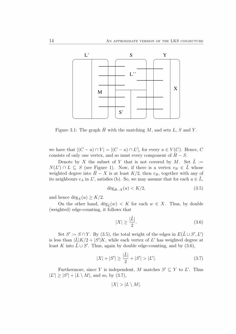
Figure 3.1: The graph H with the matching M , and sets L, S and Y .
we have that |(C − u) ∩ Y | = |(C − u) ∩ L′|, for every u ∈ V (C). Hence, Cconsists of only one vertex, and so must every component of H − S.
Denote by X the subset of Y that is not covered by M . Set L :=N(L′) ∩ L ⊆ S (see Figure 1). Now, if there is a vertex vB ∈ L whoseweighted degree into H − X is at least K/2, then vB, together with any ofits neighbours vA in L′, satisfies (b). So, we may assume that for each u ∈ L,
degH−X(u) < K/2, (3.5)
and hence degX(u) ≥ K/2.
On the other hand, degL(w) < K for each w ∈ X. Thus, by double(weighted) edge-counting, it follows that
|X| ≥ |L|2. (3.6)
Set S ′ := S ∩ Y . By (3.5), the total weight of the edges in E(L∪ S ′, L′)is less than |L|K/2 + |S ′|K, while each vertex of L′ has weighted degree atleast K into L ∪ S ′. Thus, again by double edge-counting, and by (3.6),
|X|+ |S ′| ≥ |L|2
+ |S ′| > |L′|. (3.7)
Furthermore, since Y is independent, M matches S ′ ⊆ Y to L′. Thus|L′| ≥ |S ′|+ |L \M |, and so, by (3.7),
|X| > |L \M |.
3.3 Proof of Theorem 2.3.3 15
Since |L| > N2
, this implies that M contains an edge uv with both
u, v ∈ L. We may assume that v ∈ L′ and u ∈ L. By (3.5), u has aneighbour w in X. Hence, the matching M ′ ∪ uw \ uv covers morevertices of Y than M ′ does, a contradiction to the choice of M ′.
Note that in the case K ≥ N/2 the situation in Lemma 3.2.3 is lesscomplicated. In that case, observe that clearly |S| ≤ |V (H − S)|. So, either|S| = |V (H − S)| (in which case conclusion (a) of Lemma 3.2.3 holds), orthere is a component C of H − S that has more than one vertex. Thus, asC is factor-critical, there exists an L′–L′ edge in C, and (a) holds again.
This proves the following lemma, which appeared in [1].
Lemma 3.2.4. If K ≥ N/2, then Lemma 3.2.3 always yields case (a).
In the case k ≥ n/2, this observation simplifies our proof of Theo-rem 2.3.3 considerably, as then only the simplest case needs to be treated.We shall not make use of Lemma 3.2.4 in our proof of Theorem 2.3.3.
3.3 Proof of Theorem 2.3.3
The organisation of this section is as follows. The first subsection is devotedto an outline of our proof, highlighting the main ideas, leaving out all details.In Subsection 3.3.2, assuming that we are given a host graph G and a treeT ∗ as in Theorem 2.3.3, we shall first apply the regularity lemma to G. Wethen use Lemma 3.2.3 to find a substructure of the corresponding weightedcluster graph H, which will facilitate the embedding of T ∗.
We shall prepare T ∗ for this by cutting it into small pieces in Subsec-tions 3.3.3 and 3.3.4. Then, in Subsection 3.3.5, we partition the matchinggiven by Lemma 3.2.3, according to the decomposition of the tree T ∗. InSubsection 3.3.6, we expose tools that we need for our embedding. What re-mains is the actual embedding procedure, which we divide into the two casesgiven by Lemma 3.2.3, and treat separately in Subsections 3.3.7 and 3.3.8.
3.3.1 Overview
In this subsection, we shall give an outline of our proof of Theorem 2.3.3.So, assume that we are given η > 0 and q > 0. The regularity lemmaapplied to parameters depending on η and q yields an n0 ∈ N. Now, letn ≥ n0, let k ≥ qn, let G be a graph of order n that satisfies the condition of
16 An approximate version of the LKS conjecture
Theorem 2.3.3, and let T ∗ be a tree with k edges. We wish to find a subgraphof G that is isomorphic to T ∗, i.e. we would like to embed T ∗ in G.
In order to do so, consider the weighted cluster graph H correspondingto G that is given by the regularity lemma. Denote by L ⊆ V (H) the set ofthose clusters that have degree at least (1+π′)k in H, where π′ = π′(η, q) > 0.Apply Lemma 3.2.3 to H and K := (1 + π′)k which yields vertices A,B ∈V (H) and a matching M . The rest of our proof will be divided into two cases,corresponding to the two possible conclusions (a) and (b) of Lemma 3.2.3.
As the technical details for these two cases overlap, we will not com-pletely separate them later on in the proof. In this outline, however, wethink it is more instructive to present first the easier proof for case (a), andthen turn our attention to case (b).
If the output of Lemma 3.2.3 is Case (a), then we shall decompose T ∗
into small subtrees (of order much below ηk) and a small set SD of vertices(of constant order in n), so that between any two of our subtrees lies a vertexfrom SD (the name SD stands for ‘seeds’). In fact, SD is the disjoint unionof two sets SDA and SDB, and each tree of T ∗−SD is adjacent to only oneof these two sets. Denote the set of trees adjacent to SDA by TA, and theset of trees adjacent to SDB by TB. The formal definition of SD, TA and TBcan be found in Section 3.3.3.
Next, in Section 3.3.5, we partition the matching M from Lemma 3.2.3into MA and MB. This is done in a way so that degMA
(A) is large enoughso that FA :=
⋃ TA fits into MA, and degMB(B) is large enough so that
FB :=⋃ TB fits into MB.
Finally, in Section 3.3.7, we embed SDA in A and SDB in B and use theregularity of the edges in H to embed the small trees of TA ∪ TB, one afterthe other, levelwise, into MA ∪MB. The order of this embedding procedurewill be such that the already embedded part of T ∗ is always connected.
Moreover, the structure of our decomposition of T ∗, and the fact thatwe embed the trees from TA ∪ TB in the matching edges, ensures that thepredecessor of any vertex r ∈ SDA ∪ SDB is embedded in a cluster that isadjacent to A, respectively to B (in which we wish embed r). This enablesus to embed all of SD in A ∪B, as planned.
An important detail of our embedding technique is that we shall alwaystry to balance the embedding in the matching edges, in the sense that theused part of either side should have about the same size. We only allowfor an unbalanced embedding if the degree of A resp. B into one of theendclusters of the concerned edge is already ‘exhausted’ (cf. Property () inSection 3.3.6). In practice, this means that whenever we have the choice
3.3 Proof of Theorem 2.3.3 17
into which endcluster of an edge e ∈ M we embed the root of some tree ofTA ∪ TB, we shall choose the side carefully.
In this manner, we can ensure that all of T ∗ will fit into M (or moreprecisely into the corresponding subgraph of G). This finishes the embeddingof T ∗ in case (a) of Lemma 3.2.3.
In case (b) of Lemma 3.2.3, it is not possible to partition the matchingM into MA and MB so that FA fits into MA and FB fits into MB, as incase (a). More precisely, for any partition of M into MA and MB, if degMA
(A)allows for the embedding of a forest of order t, say, in MA, then degMB∪L(B)only guarantees for the embedding of a forest of order at most (k − t)/2 inthe subgraph of Gp induced by MB and the edges incident with L′, whereL′ := L \M . For more details on this, see Lemma 3.3.1.
We use a combination of two strategies to overcome this problem. Firstly,we shall embed T ∗ in two phases, leaving for the second phase some subtreesthat are (each) adjacent to only one vertex from SD. Secondly, we shallembed some of the trees from TB in part of the matching reserved for FA.This means that we ‘switch’ some of our trees to TA.
Let us explain the two strategies in more detail. We modify our setsTA ∪ TB, in the following way. Denote by TA the set of those trees fromTA that are adjacent to only one vertex from SDA, and similarly define TB.(Observe that thus the deletion of any tree in TA ∪ TB leaves T ∗ connected.)
We may assume that
|V (⋃TA)| ≥ |V (
⋃TB)|.
Finally, set T ′ := (TA ∪ TB) \ (TA ∪ TB). Our plan now is to first embed thetrees from T ′ ∪ TB together with the vertices from SD and to postpone theembedding of FA :=
⋃ TA to a later stage. As the part of the tree embeddedin the first phase is connected, we avoid the difficulty of having to connectalready embedded parts of T ∗ in the second phase.
Now, we shall partition M into MF and MB so that degMF(A) allows for
the embedding of⋃ T ′, and degMB∪L(B) allows for the embedding of FB :=⋃ TB. This actually means that the place we reserved for the embedding of
FB − V (FB) lies in MF . Therefore, we shall ‘switch’ this forest to TA (whichis the second of our strategies).
Let us explain what we mean by switching. For each tree T ∈ TB \ TB,delete all vertices from T that are adjacent to SDB in T ∗ and add them toSDA. Put the components of what remains of T into TA. Denote the thusenlarged SDA by SD
Aand set SD := SD
A ∪ SDB.

18 An approximate version of the LKS conjecture
After switching all trees T ∈ TB \ TB, denote by TF the (enlarged) setTA \ TA. That is, TF consists of all trees from the original TA \ TA, togetherwith all trees we generated by switching. It will be easy to verify that theswitching procedure does not increase too much the number of seeds.
Also, each tree from TF and TA is adjacent only to the enlarged SDA
,and each tree from TB is still adjacent only to SDB. For details on theswitching procedure, consult Section 3.3.4.
It remains to embed T ∗ in G, which is done in Section 3.3.8. We firstembed the vertices from SD
A∪SDB in A∪B, embed FF :=⋃ TF in MF , and
embed part of TB in MB, in the same way as in case (a). In a second phase,we embed the remaining trees from TB into edges of H that are incident withL′. For each tree, we are able to find a free space in a suitable edge becauseof the high degree of the clusters from L′.
In the remaining third phase we wish to embed FA. We shall now useall of M , forgetting about the partition into MF and MB. The neighboursof the trees from TA in SD
Ahave already been embedded in the first phase.
Having chosen their images carefully then, ensures that now they have stilllarge enough degree into what is not yet used of M . Hence, there is enoughplace for FA in M .
Also, it is essential here that each edge of M meets N(A) in at most onecluster. The reason is that parts of these clusters might have been used inthe first and second phases of the embedding. So, some of the edges involvedmight be unbalanced, in the sense above, because e. g. the degree of B wassuch that we were not able to choose the endcluster in which we embeddedthe roots of the trees from TB. However, as each edge of M has at most oneendcluster in N(A), it is irrelevant whether the embedding is balanced or notin these edges.
The embedding itself of FA is done as before. This finishes the sketch ofour proof in case (b).
3.3.2 Preparations
We shall now prove Theorem 2.3.3. First of all, we fix a few constantsdepending on η and q. Set
π := minη, q, ε :=π7q
25 · 107and m0 :=
500
qπ3.
The regularity lemma (Theorem 3.2.1) applied to ε, and m0 yields nat-ural numbers M0 and N0.
3.3 Proof of Theorem 2.3.3 19
Fix
β :=ε
M0
, p :=π3q
250and n0 := max
N0,
8M0
β· 8
p
.
Thus our constants satisfy the following relations
1
n0
β ε 1
m0
< p π ≤ q,
where a b stands for the fact that a < π100b.
In particular, p satisfies
4ε+1
m0
< p =π3q
250. (3.8)
Let n ≥ n0, let k ≥ qn, and let G be a graph of order n which has at leastn2
vertices of degree at least (1+η)k. Suppose T ∗ is a tree of order k+1. Ouraim is to find an embedding ϕ : V (T ∗)→ V (G) that preserves adjacency.
Now, by Theorem 3.2.1 there exists an (ε,N)-regular partition of V (G),with m0 ≤ N ≤ M0. As in Section 3.2.1, let Gp be the subgraph of G thatpreserves exactly the edges between regular pairs of density at least p.
By (3.1) and by (3.8),
|E(G−Gp)| < pn2 ≤ π3
250kn.
Thus, for all but at most π2
50n vertices v, we have that degGp
(v) ≥ degG(v)−π5k. Hence,
Gp has at least (1− π2
25)n
2vertices of degree at least (1 +
4π
5)k.
Let H = Hp be the weighted cluster graph corresponding to Gp. Denoteby L the set of those clusters in V (H) that contain more than εs verticesof degree at least (1 + 4π
5)k in Gp. A simple calculation shows that |L| >
(1− π2
5)N
2.
Now, delete minπ2N/5, |V (H) \ L| clusters in V (H) \ L to obtaina subgraph of the cluster graph H. As this subgraph is very similar (oridentical) to H, in the rest of the text we shall denote it as well by H. Sofrom now on, by H, we shall always refer to this subgraph. Each cluster inL drops its degree by at most π2
5Ns ≤ πk
5. Thus, by (3.3), each cluster X in
L has degree
degH(X) > (1 +3π
5)k − 2εn > (1 +
π
5)k. (3.9)
20 An approximate version of the LKS conjecture
Then Lemma 3.2.3 applied to H andK := (1+π5)k yields an edgeAB ∈ E(H)
with A,B ∈ L, together with a matching M ′ of H, which satisfy (a) or (b)of Lemma 3.2.3. Obtain M from M ′ by deleting all edges that are incidentwith A or with B. In case (a) of Lemma 3.2.3, we calculate that
mindegM(A), degM(B) ≥ (1 +π
5)k − 3n
N
≥ (1 +π
5− 3
qm0
)k
≥ (1 +π
10)k. (3.10)
Similarly, in case (b) it follows that
degM(A) ≥ (1 +π
10)k and degM∪L(B) ≥ (1 +
π
10)k
2. (3.11)
Thus, for the remainder of our proof of Theorem 2.3.3 we shall work withthe assumption that there is a matching M of H and vertices A,B /∈ V (M)so that
1. degM(A), degM(B) ≥ (1 + π10
)k, or
2. degM(A) ≥ (1 + π10
)k, degM∪L(B) ≥ (1 + π10
)k2, and each cluster in N(A)
meets a different edge of M .
We shall refer to these two cases as ‘Case 1’ and ‘Case 2’, respectively.We will embed the tree T ∗ in the subgraph G′p ⊆ Gp corresponding to H,using two different strategies in Case 1 and in Case 2.
3.3.3 Partitioning the tree
In this section, we shall cut our tree into small pieces. More precisely, weshall define a set SD ⊆ V (T ∗), and sets TA and TB of disjoint small subtreesof T ∗ which are connected through the vertices from SD. Moreover, SDtogether with the union of all trees from TA ∪ TB will span T ∗.
Fix a root R of T ∗, and regard T ∗ as a poset having R as the minimalelement. For a vertex x of a subtree T ⊆ T ∗, denote by T (x) the subtreeof T induced by x and all vertices y greater than x in the tree-order of T ∗.(That is, T (x) contains all vertices y such that the path between the root Rand y contains the vertex x.) If R /∈ V (T ), then define the seed sd(T ) of Tas the maximal vertex of T ∗ which is smaller than every vertex of T .
Our sets SD = SDA ∪ SDB, TA and TB will satisfy:
3.3 Proof of Theorem 2.3.3 21
(I) SDA ∩ SDB = ∅,(II) r ∈ SD lies at even distance toR if and only if r ∈ SDA, andR ∈ SDA,
(III) TA ∪ TB consists of the components of T ∗ − SD,
(IV) |V (T )| ≤ βk, and sd(T ) ∈ SD, for each T ∈ TA ∪ TB,
(V) max|SDA|, |SDB| ≤ 2β, and
(VI) eT ∗(V (FA), SDB) = 0, and eT ∗(V (FB), SDA) = 0,
where FA :=⋃T∈TA
T and FB :=⋃T∈TB
T are the forests spanned by TAand TB.
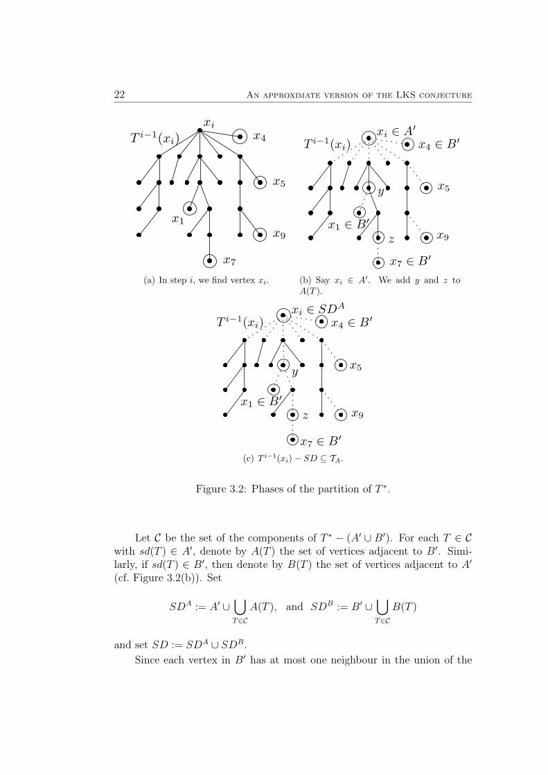
Let us first define SD. To this end, we shall inductively find vertices xi,and define auxiliary trees T i ⊆ T ∗. Set T 0 := T ∗.
In step i ≥ 1, let xi ∈ V (T ∗) be the maximal vertex in the tree-order ofV (T i−1) with
|V (T i−1(xi))| > βk, (3.12)
as illustrated in Figure 3.2(a), and define
T i := T i−1 − (T i−1(xi)− xi).
If there is no vertex satisfying (3.12), then set xi := R, and stop thedefinition process.
Say our process stops in some step j. Let A′ be the set of all xi, i ≤ j,with even distance to the root R, and let B′ be the set of all other xi.
Note that, because of (3.12), at each step i ≤ j − 1,
|V (Ti)| ≤ |V (Ti−1)| − (βk − 1),
and thus, by the definition of n0,
j − 1 ≤ |V (T ∗)|βk − 1
≤ k + 1
βk − 1≤ 3
2β.
Hence,
|A′ ∪B′| ≤ 2
β. (3.13)
For the sake of condition (VI), we shall now add a few more vertices toour sets A′ and B′, which will result in the desired SD.
22 An approximate version of the LKS conjecture
xi
T i−1(xi)
x1
x5
x9
x7
x4
(a) In step i, we find vertex xi.
T i−1(xi)xi ∈ A′
x5
x9
y
zx1 ∈ B′
x7 ∈ B′
x4 ∈ B′
(b) Say xi ∈ A′. We add y and z toA(T ).
T i−1(xi)xi ∈ SDA
x5
x9z
y
x1 ∈ B′
x7 ∈ B′
x4 ∈ B′
(c) T i−1(xi)− SD ⊆ TA.
Figure 3.2: Phases of the partition of T ∗.
Let C be the set of the components of T ∗ − (A′ ∪ B′). For each T ∈ Cwith sd(T ) ∈ A′, denote by A(T ) the set of vertices adjacent to B′. Simi-larly, if sd(T ) ∈ B′, then denote by B(T ) the set of vertices adjacent to A′
(cf. Figure 3.2(b)). Set
SDA := A′ ∪⋃T∈C
A(T ), and SDB := B′ ∪⋃T∈C
B(T )
and set SD := SDA ∪ SDB.
Since each vertex in B′ has at most one neighbour in the union of the
3.3 Proof of Theorem 2.3.3 23
A(T ), it follows that|SDA \ A′| ≤ |B′|,
and analogously,|SDB \B′| ≤ |A′|.
Thus,max|SDA|, |SDB| ≤ |A′ ∪B′|. (3.14)
Finally, we shall define TA and TB. Let C ′ be the set of the componentsof T ∗ − SD. Set
TA := T ∈ C ′ : sd(T ) ∈ SDA and TB := T ∈ C ′ : sd(T ) ∈ SDB,
as shown in Figure 3.2(c), and define the forests
FA :=⋃T∈TA
T and FB :=⋃T∈TA
T.
Observe that Conditions (I)–(IV) and (VI) are clearly met and that (V)holds because of (3.13) and (3.14).
This finishes our manipulation of the tree T ∗ in Case 1.
3.3.4 The switching
In Case 2 from Section 3.3.2, we shall not only cut our tree to small pieces(cf. Section 3.3.3), but also switch some of our small subtrees from one of thetwo sets TA, TB to the other. We achieve this by adding some more verticesto SD, thus naturally refining our partition of T ∗.
Set
TA :=T ∈ TA : e(V (T ), SD − sd(T )) = ∅, and
TB :=T ∈ TB : e(V (T ), SD − sd(T )) = ∅.
We may assume that
|⋃T∈TA
V (T ) | ≥ |⋃T∈TB
V (T ) |. (3.15)
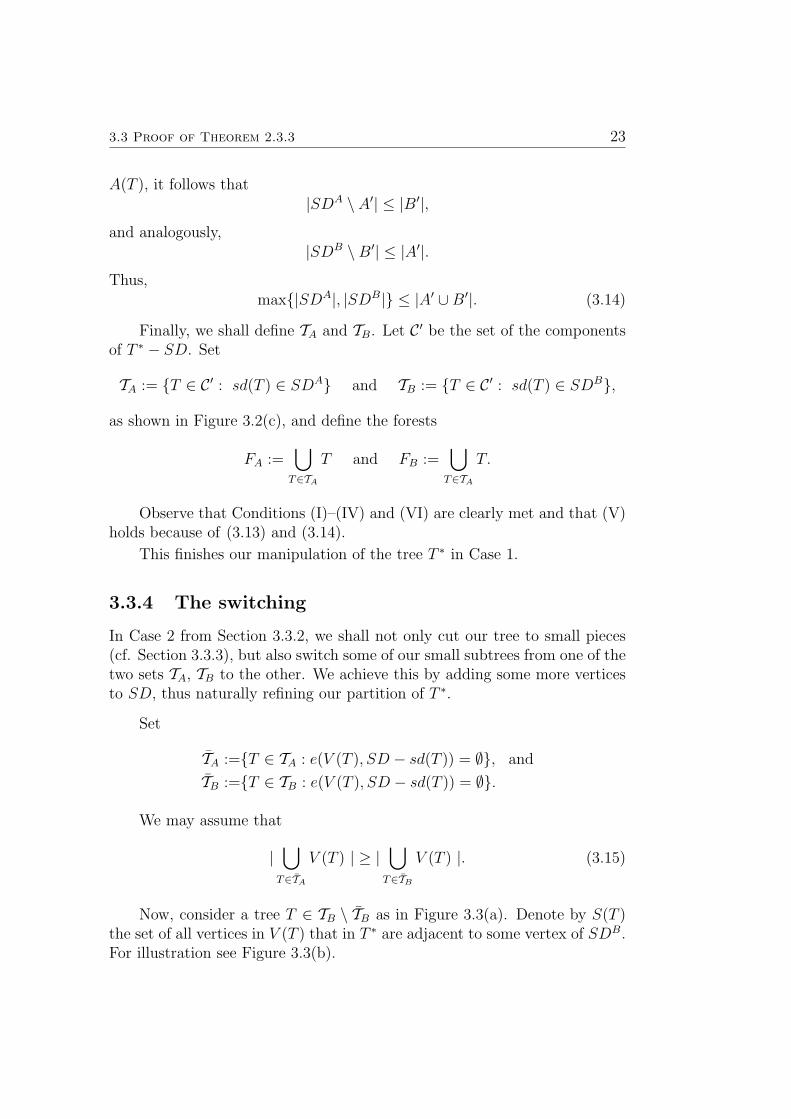
Now, consider a tree T ∈ TB \ TB as in Figure 3.3(a). Denote by S(T )the set of all vertices in V (T ) that in T ∗ are adjacent to some vertex of SDB.For illustration see Figure 3.3(b).
24 An approximate version of the LKS conjecture
T
sd(T )
v1 v2 v3
v4
(a) A tree T ∈ TB \ TB , withsd(T ), x1, x2, x3, x4 ∈ SDB .
T
sd(T )
v1 v2 v3
v4
u2 u3
u4
u1
(b) The set S(T ) = y1, . . . , y4, andthe subtrees of T generated by theswitching.
Figure 3.3: The switching procedure.
Set
SDA
:= SDA ∪⋃
T∈TB\TB
S(T ) and SD := SDA ∪ SDB.
Finally, define
T ′A :=⋃
T∈TB\TB
C : C is a component of T − S(T )
andTF := (TA \ TA) ∪ T ′A.
(The F in TF stands for ‘first’, as this part of the tree is to be embeddedfirst.) Finally, set
FF :=⋃T∈TF
T,
FA :=⋃T∈TA
T and FB :=⋃T∈TB
T.

3.3 Proof of Theorem 2.3.3 25
Observe that our sets SD = SDA ∪ SDB, TF ∪ TA, and TB still satisfy
conditions (I)-(IV) and (VI) from Section 3.3.3 (with SD, SDA, TA, TB,
FA, and FB replaced by SD, SDA
, TF ∪ TA, TB, FA, and FB, respectively).Instead of (V), we now have the similar
(V)’ |SD| ≤ 8β,
since by the definition of SDA
we know that for each vertex x of SDB, wehave created at most 2 vertices of SD
A\SDA (between x and the next vertexof SDB in direction of the root R). Thus,
|SDA| ≤ |SDA|+ 2|SDB| ≤ 6
β,
as needed for (V)’.
3.3.5 Partitioning the matching
In this subsection, we shall divide the matching M into two parts, into whichwe will later embed the two forests FA, FB, respectively FF and FB, of T ∗
that we defined in Subsection 3.3.3, resp. in Subsection 3.3.4. (The forest FAwill be embedded later).
For this, we will need the following number-theoretic lemma, which ap-peared also in [1]. We give a short proof.
Lemma 3.3.1. Let I be a finite set, and let a, b,∆ > 0. For i ∈ I, letai, bi ∈ (0,∆]. Suppose that
a∑i∈I ai
+b∑i∈I bi
≤ 1. (3.16)
Then there is a partition of I into Ia and Ib such that∑
i∈Ia ai > a−∆ and∑i∈Ib bi ≥ b.
Proof. Define a total order on I in a way that i j implies ai
bi≤ aj
bjfor all
i, j ∈ I. Let ` ∈ I be minimal in this order with a ≥∑i` ai.
Set Ia := i ∈ I : i ` and set Ib := I \ Ia. It is clear that∑
i∈Ia ai >a−∆, by the definition of ` and as a` ≤ ∆. So, all we have to show is that∑
i∈Ib bi ≥ b.
26 An approximate version of the LKS conjecture
Indeed, suppose otherwise. Then by (3.16), and by the definition of `,we have that ∑
i∈Ib bi∑i∈I bi
<b∑i∈I bi
≤ a−∑i∈Ia ai∑i∈I ai
+b∑i∈I bi
≤ 1−∑
i∈Ia ai∑i∈I ai
=
∑i∈Ib ai∑i∈I ai
.
Multiply the two sides of this inequality with∑
i∈I ai ·∑
i∈I bi, subtractthe term
∑i∈Ib ai ·
∑i∈Ib bi, and divide by
∑i∈Ia bi
∑i∈Ib bi to obtain
a`b`≤∑
i∈Ia ai∑i∈Ia bi
<
∑i∈Ib ai∑i∈Ib bi
≤ a`b`,
(where the first and last inequality follow from the definition of ). Thisyields the desired contradiction.
We shall now apply Lemma 3.3.1 to partition our matchingM = eii≤|M |.We do this separately for the two cases from Section 3.3.2.
In Case 1, we set
a := |V (FA)|+ πk
20, b := |V (FB)|+ πk
20, and ∆ := 2s.
For i ≤ |M |, set ai := degei(A) ≤ ∆, and bi := degei
(B) ≤ ∆. Now, (3.10)implies that
a∑|M |i=1 ai
+b∑|M |i=1 bi
≤ |V (FA)|+ |V (FB)|+ πk10
(1 + π10
)k≤ 1.
Hence, Lemma 3.3.1 yields a partition of M into MA and MB such that
degMA(A) > |V (FA)|+ πk
40and degMB
(B) > |V (FB)|+ πk
40. (3.17)
In Case 2, set
a := |V (FF )|+ πk
20, b := |V (FB)|+ πk
40, and ∆ := 2s.
3.3 Proof of Theorem 2.3.3 27
For i = 1, . . . , |M |, again set ai := degei(A), and bi := degei
(B). Set L′ :=L \M . For i = |M | + 1, . . . , |M | + |L′|, set ai := 0, and set bi := degCi
(B),where Ci is the ith cluster in L′.
Observe that by (3.15),
|V (FB)| ≤ k − |V (FF )|2
. (3.18)
Now, let us check that the conditions of Lemma 3.3.1 hold. Clearly,ai, bi ≤ ∆ for all i ≤ |M |+ |L′|.
Moreover, Condition (3.16) holds since (3.11) and (3.18) imply that
a∑|M |+|L′|i=1 ai
+b∑|M |+|L′|
i=1 bi≤ |V (FF )|+ πk
20
(1 + π10
)k+|V (FB)|+ π
40
(1 + π10
)k2
≤ |V (FF )|+ 2|V (FB)|+ πk10
(1 + π10
)k
≤ 1.
We thus obtain a partition of M into MF and MB such that
degMF(A) > |V (FF )|+ πk
40and degMB∪L′(B) ≥ |V (FB)|+ πk
40. (3.19)
Let T MB ⊆ TB be maximal with
degMB(B) ≥ |
⋃T∈TM
B
V (T )|+ πk
40N|MB|. (3.20)
Set T LB := TB \ T MB . Let FMB :=
⋃T∈TM
BT and let FL
B := FB − V (FMB ).
Observe that if T MB 6= TB, then the maximality of T MB ensures that
degMB(B) < |V (FM
B )|+ πk
40N|MB|+ βk.
Hence, by (3.19), either T LB = ∅, or
degL′(B) ≥ |V (FLB )|+ πk
80N|L′|. (3.21)
28 An approximate version of the LKS conjecture
3.3.6 Embedding lemmas for trees
In this section, we shall prove some preparatory lemmas on embedding treesin regular pairs of H.
Let C,D ∈ V (H), and let U,N ⊆ C∪D. We say that U has Property (?)in CD for N if it satisfies the following.
(?) If ||C ∩ U | − |D ∩ U || > βk + εs, thenmin|N ∩ C|, |N ∩D| ≤ min|C ∩ U |, |D ∩ U |+ 2εs+ βk.
Lemma 3.3.2. Let (T, r) be a rooted tree of order at most βk. Let CD ∈E(H). Suppose that U,N ⊆ C ∪D are such that
min|N ∩ C \ U |, |D \ U | > 2
p(εs+ βk).
Then there is an embedding ϕ of T in (C ∪D) \ U such that ϕ(r) ∈ N andsuch that the following holds.
(??) If U has Property (?) in CD for N ,then also Uϕ := U ∪ ϕ(V (T )) has Property (?) in CD for N .
Proof. Write V (T ) = r ∪ L1 ∪ L2 ∪ . . ., where L` is the `th level of T (i. e.the set of vertices at distance ` to r).
First, suppose that |N∩D\U | ≤ εs. In this case, choose ϕ(r) ∈ N∩C\Utypical w. r. t. D \ U . (This is possible, as by (3.2), there are at most εsvertices that are not typical.)
Embed the rest of V (T ) levelwise, choosing for ϕ(L`) unused vertices ofD\U that are typical with respect to C \U , if ` is odd; and choosing verticesof C \ U that are typical with respect D \ U , if ` is even.
Now, suppose that |N ∩D \ U | > εs. In this case, we may alternativelywish to embed r in N ∩D. We do so in either of the following cases
1. |⋃`∈N L2`−1| > |⋃`∈N L2`| and |C \ U | ≥ |D \ U |, or
2. |⋃`∈N L2`−1| < |⋃`∈N L2`| and |C \ U | ≤ |D \ U |,
and otherwise embed r in N ∩C, as before. After having thus chosen a placefor the root r, the rest of T is embedded analogously as above (possiblyswapping the roles of C and D). We have thus completed the embedding ofT .
It remains to prove (??). So assume that Uϕ has Property (?) for N insome edge CD. Furthermore, assume that
||C ∩ Uϕ| − |D ∩ Uϕ|| > βk + εs. (3.22)
3.3 Proof of Theorem 2.3.3 29
Now, if ||C ∩U | − |D ∩U || > βk+ εs, then Property (?) for Uϕ follows fromProperty (?) for U . So suppose otherwise, that is
||C ∩ U | − |D ∩ U || ≤ βk + εs. (3.23)
By (3.22), this means that we could not choose into which of N ∩ C andN ∩D we would embed the root of T . Hence,
minY=C,D
|N ∩ Y \ U | ≤ |N ∩D \ U | ≤ εs.
Using (3.23), this gives
min|N ∩ C|, |N ∩D| ≤ max|C ∩ U |, |D ∩ U |+ minY=C,D
|N ∩ Y \ U |≤ max|C ∩ U |, |D ∩ U |+ εs
≤ min|C ∩ U |, |D ∩ U |+ 2εs+ βk
≤ min|C ∩ Uϕ|, |D ∩ Uϕ|+ 2εs+ βk,
as desired.
Let C,D,X ∈ V (H), let X ′ ⊆ X, let Z ⊆ V (H), let U ⊆ ⋃V (H), letm ∈ N, and let (T, r) be a rooted tree.
We say that U has Property () in (C,D) with respect to X if it satisfiesthe following.
() If ||C ∩ U | − |D ∩ U || > βk, thenmindegC(X), degD(X) ≤ min|C ∩ U |, |D ∩ U |+ 5εs+ βk.
An embedding ϕ of T is a (v,X ′, U)-embedding in Z, if ϕ(V (T ) \ r) ⊆⋃Z \ U , if ϕ(r) = v, and if each vertex at odd distance to the root r ismapped to a vertex that is typical to X ′.
A vertex is Z-typical, if it is typical to each cluster from Z.
The set Z is said to be (m,U)-large for X, if
degZ(X) > m+ |U ∩⋃Z|+ πk
100N|Z|.
Lemma 3.3.3. Let (T, r), X ′, X and U be as above with |X ′| ≥ |X|/2.A) Suppose MX is a matching in H −X so that V (MX) is (|V (T )|, U)-largefor X, so that v ∈ X is V (MX)-typical, and so that U has Property () in(C,D) with respect to X, for each CD ∈MX .Then, there is a (v,X ′, U)-embedding ϕ of T in V (MX) such that U∪ϕ(V (T ))has Property () with respect to X for every CD ∈MX .B) Let LX , NLX
⊆ V (H) be such that LX is (|V (T )|, U)-large for X, andNLX
is (|V (T )|, U)-large for each Y ∈ LX . If v ∈ X is LX-typical, then thereis a (v,X ′, U)-embedding ϕ of T in LX ∪NLX
.
30 An approximate version of the LKS conjecture
Proof. We map r to v and embed the trees from the forest F := T − rinductively. In each step j ≥ 1, we embed a tree T j of the forest F . Denoteby V <j ⊆ V (F ) the set
⋃i<j V (T i) of vertices we have already embedded
before step j. Let S be the set of vertices in⋃V (H) that are not typical to
X ′. Set U<j := U ∪ S ∪ ϕ(V <j). In particular, U<1 = U ∪ S.
For Part A), we shall moreover use two properties of U during ourembedding. Firstly, if CD ∈MX satisfies ||C ∩ U | − |D ∩ U || ≤ βk, then werequire that in each step j ≥ 1
(I) U<j has Property ( ? ) for N(v) ∩ (C ∪D).
This property holds for j = 1, as the condition of Property (?) is void, andwe shall check it for each later step.
Secondly, for the edges with ||C ∩ U | − |D ∩ U || > βk, observe that, asthe sets U<j are growing, Property () ensures that for all j ≥ 1
(II) minY ∈C,DdegY (X) ≤ minY ∈C,D|Y ∩ U<j|+ 5εs+ βk.
So, assume now that we are in step j ≥ 1, that is, ϕ(x) has been definedfor all x ∈ V <j, and we are about to embed T j.
Claim 3.3.4. There is an edge CD, with CD ∈ MX for Part A) and withC ∈ L, for Part B), such that
min|(N(v) ∩ C) \ U<j|, |D \ U<j| ≥ 2
p(εs+ βk).
Before proving Claim 3.3.4, we shall show how we complete our embed-ding of T j under the assumption that the claim holds for the edge e = CD.
Set N := N(v) ∩ e and let rj := N(r) ∩ V (T j) be the root of T j. ApplyLemma 3.3.2 to embed (T j, rj) in e\U<j, mapping rj to N(v). Lemma 3.3.2together with (I) for j ensures (I) for j + 1. As our embedding avoids S, allvertices in ϕ(T ) are typical to X ′. This terminates step j.
Say we terminate the embedding procedure in step `. Then ϕ is a(v,X ′, U)-embedding. So, for Part B), we are done. For Part A), however,we still have to prove that U<` \ S has Property () in each CD ∈MX .
To this end, assume that ||C ∩ (U<` \ S)| − |D ∩ (U<` \ S)|| > βk. If||C ∩ U | − |D ∩ U || ≤ βk, then by (I), U<` has Property (?) in CD forN(v) ∩ (C ∪D). Hence,
minY=C,D
degY (X) ≤ minY=C,D
degY (v)+ 2εs
≤ minY=C,D
|Y ∩ (U<`)|+ 4εs+ βk
≤ minY=C,D
|Y ∩ (U<` \ S)|+ 5εs+ βk.
3.3 Proof of Theorem 2.3.3 31
On the other hand, if ||C ∩ U | − |D ∩ U || > βk, then (II) ensures that
minY ∈C,D
degY (X) ≤ minY ∈C,D
|Y ∩ (U<` \ S)|+ 5εs+ βk.
This shows that U<` \ S has Property () in each CD ∈MX for Part A). Itonly remains to prove Claim 3.3.4.
Proof of Claim 3.3.4: First, suppose we are in Case A). Let us startby showing that there is an edge e = CD ∈MX which satisfies
dege(X)− |e ∩ U<j| ≥ 8
p(εs+ βk) + 2εs. (3.24)
Indeed, suppose there is no such edge. Then, as V (MX) is (V (T ), U)-large,we have that
8
p(εs+ βk)|MX | >
∑e∈MX
(dege(X)− |e ∩ U<j| − 2εs)
= degMX(X)− |U ∩
⋃MX | − |U<j \ U | − 2εs|MX |
≥ degMX(X)− |U ∩
⋃MX | − |V (T )| − |S ∩MX | − 2εs|MX |
≥ πk
100N|V (MX)| − 4εs|MX |
>πk
100N|MX |,
which, as βk ≤ εM0n ≤ εs, implies that 16ε/p > πq/100, a contradiction.
So, assume now that we have chosen an edge e for which (3.24) holds.Clearly, we can write e = CD such that
4
p(εs+ βk) ≤ degC(X)− 2εs− |C ∩ U<j| ≤ |N(v) ∩ C \ U<j|. (3.25)
We claim that
|D \ U<j| ≥ 2
p(2εs+ βk). (3.26)
Indeed, suppose for contradiction (3.26) does not hold. Then (3.25) impliesthat
|C ∩ U<j| ≤ s− 4
p(εs+ βk)
= |D ∩ U<j|+ |D \ U<j| − 2
p(2εs+ βk)− 2
pβk
≤ |D ∩ U<j| − 2
pβk.
32 An approximate version of the LKS conjecture
Hence, either by (I), or by (II), it holds that
mindegC(X), degD(X) ≤ |C ∩ U<j|+ 5εs+ βk.
Thus, by (3.24),
8
p(εs+ βk) + 2εs ≤ dege(X)− |C ∩ U<j| − |D ∩ U<j|
≤ dege(X)−mindegC(X), degD(X)+ 5εs+ βk − |D ∩ U<j|≤ s+ 5εs+ βk − |D ∩ U<j|< |D \ U<j|+ 5εs+ 2βk.
So, |D\U<j| > (8p−3)(εs+βk), a contradiction to our assumption that (3.26)
does not hold. This proves (3.26), which together with (3.25) then impliesClaim 3.3.4 for Case A).
Now, assume that we are in Case B). First we show that if some Z ⊆V (H) is (|V (T )|, U)-large for some Y ∈ V (H), then there is a Z ∈ Z ∩N(Y )such that
degZ(Y )− |Z ∩ U<j| ≥ 2
p(εs+ βk) + 2εs.
Indeed, otherwise
2
p(εs+ βk)|Z| >
∑Z∈Z
(degZ(Y )− |Z ∩ U<j| − 2εs)
≥ degZ(Y )− |U<j ∩⋃Z| − 2εs|Z|
> (πk
100N− 4εs)|Z|
≥ πk
200N|Z|,
a contradiction, as above.
So there is a C ∈ LX and a D ∈ NLX∩N(C) such that
|N(v) ∩ C \ U<j| ≥ degC(X)− |C ∩ U<j| − 2εs ≥ 2
p(εs+ βk)
and
|D \ U<j| ≥ degD(C)− |D ∩ U<j| ≥ 2
p(εs+ βk),
as desired for Claim 3.3.4.
3.3 Proof of Theorem 2.3.3 33
3.3.7 The embedding in Case 1
In this subsection, we shall complete the proof of Theorem 2.3.3 under theassumption that Case 1 of Section 3.3.2 holds. So, we assume that there arean edge AB ∈ E(H) and a matching M = MA ∪MB in H − A,B as inSection 3.3.5. These, together with the sets SD = SDA ∪ SDB, TA and TBfrom Section 3.3.3, satisfy (3.17).
Our embedding ϕ will be defined in |SD| steps. In each step i ≥ 1, wechoose a suitable vertex ri ∈ SD and embed it together with all trees from
Ti := T ∈ TA ∪ TB : sd(T ) = ri.
Set V0 := ∅ and for i ≥ 1, let
Vi := Vi−1 ∪ ri ∪⋃T∈Ti
V (T ).
We start with r1 := R, and in each step i > 1, we shall choose a vertexri ∈ SD \ Vi−1 that is adjacent to Vi−1. The seed ri will be embedded ina vertex vi ∈ A ∪ B, while Ti will be mapped to edges from M (or moreprecisely, to the corresponding subgraph of G′p). Set U0 := ∅, and once ϕ isdefined on Vi, set Ui := ϕ(Vi).
For each i ≥ 0, the following conditions will hold.
(i) |(A ∪B) ∩ Ui| ≤ i,
(ii) if x ∈ Vi ∩N(SDA), resp. x ∈ Vi ∩N(SDB), then ϕ(x) has at least p4s
neighbours in A, resp. in B,
(iii) for CD ∈MA, the set Ui has Property () in CD with respect to A.
(iv) for CD ∈MB, the set Ui has Property () in CD with respect to B.
Observe that properties (i)–(iv) trivially hold for i = 0.
So, suppose now that we are in some step i ≥ 1 of our embedding process.Choose ri ∈ SD as detailed above. Let us assume that ri ∈ SDA, the casewhen ri ∈ SDB is analogous.
We embed ri in a vertex vi = ϕ(ri) ∈ A that is typical with respect toB and typical w. r. t. all but at most 2
√ε|MA| clusters of MA. Properties (i)
and (ii) for i− 1 ensure that if x is the predecessor of ri in T ∗, then ϕ(x) hasat least ps
4− i neighbours in A \ Ui−1. By (3.2) and (3.4), at most 2
√εs of

34 An approximate version of the LKS conjecture
these vertices do not have the required properties. Hence, there are at least(p
4− 2√ε)s− i ≥ 1 suitable vertices we may choose vi := ϕ(ri) from.
LetM iA ⊆MA be a maximal submatching such that vi is typical w. r. t. each
of the end-clusters of each edge of M iA. Then by (3.4) and (3.17) we obtain
degM iA
(A) ≥ degMA(A)− 4
√ε|MA|s
> |V (FA)|+ πk
40− 4√ε|MA|s
> |V (FA)|+ πk
80
> |V (⋃Ti)|+ |Ui−1 ∩
⋃V (MA)|+ πk
80N|V (M i
A)|.
Now we use Lemma 3.3.3 Part A) letting (T, r) be the tree induced byri and the trees from Ti, and setting MX := M i
A, U := Ui−1, v := vi, andX = X ′ = A. It is easy to see that (i), (ii), and (iv) hold for i, as they holdfor i− 1, and by our choice of ϕ(Vi \Vi−1). Lemma 3.3.3 Part A) ensures ()for all edges CD ∈M i
A. As we did not embed anything in the edges outsideM i
A, (iii) for i− 1 implies (iii) for i, for all CD ∈MA.
This completes the embedding of the tree T ∗ in G′p ⊆ G in Case 1.
3.3.8 The embedding in Case 2
We shall now complete the proof of Theorem 2.3.3 under the assumption thatCase 2 of Section 3.3.2 holds. That is, there are an edge AB ∈ E(H) and a
matching M = MF∪MB in H−A,B together with sets SD = SDA∪SDB,
TF , TA, T MB and T LB from Sections 3.3.3 and 3.3.4 satisfying (3.20) and (3.21)from Section 3.3.5.
Our embedding will be defined in three phases. In the first phase, weshall embed all vertices from SD in A ∪ B, embed FF in edges of MF , andembed FM
B in edges of MB. In the second phase, we shall embed FLB in edges
incident with L′ ∩ N(B), and in the third phase, we shall embed FA in theremaining space inside edges from M .
Denote by A′ the set of vertices in A that are typical to all but at most2√ε|M | clusters of V (M), and denote by B′ the set of vertices in B that are
typical to all but at most√ε|L′| clusters of L′.
The first phase is done analogously as in Case 1, always considering A′
and B′ instead of A and B. In each step, Lemma 3.3.3 Part A) is used inthe following setting.
3.3 Proof of Theorem 2.3.3 35
The rooted tree (T, r) is the tree induced by ri and the trees from
Ti := T ∈ TF ∪ T MB : sd(T ) = ri.
We set either (X ′, X) = (A′, A) or (X ′, X) = (B′, B), and let v = ϕ(ri). Thematching MX is a maximal submatching either of MF or of MB, so that ϕ(ri)is V (MX)-typical. Finally, the set U is the set of the vertices used beforestep i.
For the second phase, assume that V (FLB ) 6= ∅ (otherwise we shall skip
the second phase). We define the second phase of our embedding process in|SDB| steps.
In each step i ≥ 1, we embed the trees T i := T ∈ T LB : sd(T ) = riin edges incident with L′. (Recall that L′ = L \M .) Suppose that we areat step i of this procedure, i. e. that we have already embedded the treesfrom T 1, . . . , T i−1. Denote by Ui−1 the set of vertices used so far for theembedding. Let L′i be the set of those clusters of L′ to which ϕ(ri) is typical.As ϕ(ri) ∈ B′, (3.4) and (3.21) imply that
degL′i(B) ≥ |V (⋃T i)|+ |Ui−1 ∩ L′i|+
πk
100N|L′i|.
Furthermore, by (3.9), for all Y ∈ L′i we have that
deg(Y ) ≥ |V (⋃T i)|+ |Ui−1|+ πk
100.
Use Lemma 3.3.3 Part B) to embed Ti, letting the rooted tree be thetree induced by ri and the trees from T i, and setting X := B, X ′ := B′,v := ϕ(ri), LX := L′i, NLX
:= N(L′i), and U := Ui−1.
The third phase of our embedding process takes place in |SDA| steps,where in each step i ≥ 1, we embed the trees from T i := T ∈ TA : sd(T ) =ri. Suppose that we are at step i of this procedure, i. e. that we have alreadyembedded the trees from T 1, . . . , T i−1. Denote by Ui−1 the set of verticesused so far for the embedding. Let Mi be the maximal submatching of Msuch that ϕ(ri) is typical to all cluster of V (Mi). As ϕ(ri) ∈ A′, we haveby (3.4) and (3.10) that
degMi(A) ≥ |V (
⋃T i)|+ |Ui|+ πk
100.
Observe that, as each edge CD ∈ M meets N(A) in at most one end-cluster, the set Ui trivially has Property () in CD with respect to A. We
36 An approximate version of the LKS conjecture
use Lemma 3.3.3 Part A) to embed Ti, letting (T, r) be the tree induced byri together with the trees from T i, and setting X := A, X ′ := A′, v := ϕ(ri),MX := Mi, and U := Ui−1.
This terminated our embedding of T ∗, and thus the proof of Theo-rem 2.3.3.
3.4 Proof of Theorem 3.1.1
Our proof of Theorem 3.1.1 follows closely the lines of the proof of Theo-rem 2.3.3. We embed a rooted spanning tree (T ∗, R) of Q, and choosing ϕcarefully, we ensure the adjacencies for the edges from E(Q) \ E(T ∗).
Proof of Theorem 3.1.1. Set π := minη, q and set
ε′ :=εc+1
c+ 4, and m0 :=
500
π2q,
where ε is the constant from the proof of Theorem 2.3.3. As in the proofof Theorem 2.3.3, the regularity lemma applied to ε′, and m0, yields naturalnumbers N0 and M ′
0. Set M0 := maxM ′0, c, define β and p accordingly,
and set
n0 := max
N0,
9M0
β·(
8
p
)c+1.
Now, let G be a graph on n ≥ n0 vertices which satisfies the condition ofTheorem 3.1.1, let k ≥ qn, and let Q be a connected bipartite graph of orderk+ 1 with at most k+ c edges, with a spanning tree T ∗. Fix a root R in T ∗.Denote by M∗ the subgraph of Q induced by the edges in E(Q) \E(T ∗) andlet N∗ be the set of predecessors of V (M∗) in the tree order of T ∗.
We decompose T ∗ as in Section 3.3.3, with the difference that we nowadd the vertices from V (M∗)∪N∗ to the sets A′ and B′ (from the definitionof SD), depending on the parity of their distance in T ∗ to R. In this way,and since Q is bipartite, we obtain, after the switching, two independentsets SD
Aand SDB so that
|SDA|+ |SDB| ≤ 8
β+ 8c <
9
β,
which is constant in n.
The definition of our the embedding ϕ is similar as in the proof ofTheorem 2.3.3, except for some extra precautions we take for vertices from
3.4 Proof of Theorem 3.1.1 37
V (M∗) ∪N∗. At step i, for each vertex r ∈ SDA, define
N ir :=
j⋂`=1
N(ϕ(x`)) ∩ A,
where x1, . . . xj are the already embedded neighbours of r in SDA
. If none of
the neighbours of r in SDA
has been embedded before step i, then set N ir :=
A. Analogously define N ir for r ∈ SDB.
In each step i of our embedding process, we shall ensure the following.
(i) If r ∈ V (M∗) is not yet embedded, then |N ir| ≥
(p4
)js,
where j = j(r, i) is the number of neighbours of r in SDA
resp. SDB
that have already been embedded before step i.
Observe that in step i = 0, either N0r = A or N0
r = B, and thereforecondition (i) is met.
Suppose that at step i ≥ 1 of our embedding process, we are about toembed a vertex r = ri ∈ V (M∗)∪N∗. Assume that r ∈ SDA
(the case whenr ∈ SDB is analogous). Denote by x1, . . . , x` the neighbours of r in V (M∗)that have not been embedded yet.
Now, embed r in a vertex from N i−1r that satisfies the at most 3 con-
ditions of typicality from the proof of Theorem 2.3.3, except the typicalityw. r. t. B, which we replace with typicality w. r. t. each N i−1
xj, for 1 ≤ j ≤ `.
This is possible, since our embedding scheme and the condition on the num-ber of edges of Q ensure that r has at most c + 1 neighbours in Q that arealready embedded. Thus, it follows from (i) for i − 1 and for r, from (3.2),and from the choice of n0 that there are at least
((p4
)c+1
− (c+ 3)ε′)s− |SD|+ 1 ≥ 1
2
(p4
)c+1
s− 9
β+ 1 ≥ 1
unused typical vertices we can choose ϕ(r) from.
Finally, observe that since we chose ϕ(r) typical w. r. t. each N i−1xj
, wehave ensured property (i) for i and for every r′ ∈ V (M∗) that is not yetembedded. This completes the proof of Theorem 3.1.1.
38 An approximate version of the LKS conjecture
Chapter 4
Solution of the LKS conjecturefor special classes of trees
4.1 Trees of small diameter and caterpillars
In this section, which is based on work from [75] we will prove the Loebl–Komlos–Sos conjecture for two classes of trees.
The first class of trees for which we shall prove Conjecture 2.1.2, is theclass of all tress that have diameter at most 5. Our result implies the resultsof Barr and Johansson [3], and Sun [87].
Theorem 4.1.1.[75] Let k, n ∈ N, and let G be a graph of order n so thatat least n/2 vertices of G have degree at least k.Then every tree of diameter at most 5 and with at most k edges is a subgraphof G.
The second of the classes for which we shall prove Conjecture 2.1.2is a subclass of the caterpillars. This extends results of Bazgan, Li, andWozniak [4].
Let T (k, `, c) be the class of all trees with k edges which can be obtainedfrom a path P of length k − `, and two stars S1 and S2 by identifying thecentres of the Si with two vertices that lie at distance c from each other onP .
Theorem 4.1.2. [75] Let k, `, c, n ∈ N such that ` ≥ c. Suppose that c iseven, or that ` + c ≥ bn/2c + 1. Let T ∈ T (k, `, c), and let G be a graph oforder n so that at least n/2 vertices of G have degree at least k.Then T is a subgraph of G.

40 Solution of the LKS conjecture for special classes of trees
4.2 Proof of Theorem 4.1.1
We shall prove the Theorem 4.1.1 by contradiction. So, assume that there arek, n ∈ N, and a graph G with |V (G)| = n, such that at least n/2 vertices ofG have degree at least k. Furthermore, suppose that T is a tree of diameterat most 5 with |E(T )| ≤ k such that T 6⊆ G.
We may assume that among all such counterexamples G for T , we havechosen G edge-minimal. In other words, we assume that the deletion of anyedge of G results in a graph which has less than n/2 vertices of degree k.
Denote by L the set of those vertices of G that have degree at least k,and set S := V (G) \ L. Observe that, by our edge-minimal choice of G,we know that S is independent. Also, we may assume that S is not empty(otherwise T ⊆ G trivially).
Clearly, our assumption that T 6⊆ G implies that for each set M of leavesof T it holds that
there is no embedding ϕ of V (T ) \M in V (G) so that ϕ(N(M)) ⊆ L.(4.1)
In what follows, we shall often use the fact that both the degree of avertex and the cardinality of a set of vertices are integers. In particular,assume that a, b ∈ N, and x ∈ Q. Then the following implication holds.
If a < x+ 1 and b ≥ x, then a ≤ b. (4.2)
Let us now define a useful partition of V (G). Set
A := v ∈ L : degL(v) <k
2,
B := L \ A,C := v ∈ S : deg(v) = degL(v) ≥ k
2, and
D := S \ C.
Let r1r2 ∈ E(T ) be such an edge that each vertex of T has distance atmost 2 to at least one of r1, r2. Set
V1 := N(r1) \ r2, V2 := N(r2) \ r1,W1 := N(V1) \ r1, W2 := N(V2) \ r2.
Furthermore, set
V ′1 := N(W1) and V ′2 := N(W2).
4.2 Proof of Theorem 4.1.1 41
Observe that |V1 ∪ V2 ∪W1 ∪W2| < k. So, without loss of generality(since we can otherwise interchange the roles of r1 and r2), we may assumethat
|V2 ∪W1| < k
2. (4.3)
Since |V ′1 | ≤ |W1|, this implies that
|V ′1 ∪ V2| < k
2. (4.4)
Now, assume that there is an edge uv ∈ E(G) with u, v ∈ B. We shallconduct this assumption to a contradiction to (4.1) by proving that then wecan define an embedding ϕ so that ϕ(V ′1 ∪ V2 ∪ r1, r2) ⊆ L. Define theembedding ϕ as follows. Set ϕ(r1) := u, and set ϕ(r2) := v. Map V ′1 to asubset of N(u)∩L, and V2 to a subset of N(v)∩L that is disjoint from ϕ(V ′1).This is possible, as (4.2) and (4.4) imply that |V ′1 ∪ V2|+ 1 ≤ degL(v).
We have thus reached the desired contradiction to (4.1). This provesthat
B is independent. (4.5)
SetN := N(B) ∩ L ⊆ A.
We claim that each vertex v ∈ N has degree
degL(v) <k
4. (4.6)
Then, (4.5) and (4.6) together imply that
|B|k2≤ e(N,B) ≤ |N |k
4,
and hence,
|N | ≥ 2|B|. (4.7)
In order to see (4.6), suppose otherwise, i. e., suppose that there is avertex v ∈ N with degB(v) ≥ k
4. Observe that by (4.4), |V ′1 ∪ V ′2 | < k
2and
hence we may assume that at least one of |V ′1 |, |V ′2 |, say |V ′1 |, is smaller thank4. The embedding ϕ is defined as for the proof of (4.5), by embedding firstV ′1 ∪r2 in N(v) and then V ′2 in a subset N(ϕ(r2))∩L, that is disjoint fromϕ(V ′1). The case when |V ′2 | < k
4is done analogously. This yields the desired
contradiction to (4.1), and thus proves (4.6).
42 Solution of the LKS conjecture for special classes of trees
Now, set
X := v ∈ L : degC∪L(v) ≥ k
2 ⊇ B.
We claim that the number of edges between X and C
e(X,C) = 0. (4.8)
Observe that thenX = B, (4.9)
and,e(B,C) = 0. (4.10)
In order to see (4.8), suppose for contradiction that there exists an edgeuv of G with u ∈ X and v ∈ C. We define an embedding ϕ of V ′1 ∪ V2 ∪WC
1 ∪ r1, r2 in V (G), where WC1 is a certain subset of W1, as follows.
Set ϕ(r1) := u, and set ϕ(r2) := v. Embed a subset V C1 of V ′1 in N(u)∩C,
and a subset V L1 = V ′1 \ V C
1 in N(u) ∩ L. We can do so because of (4.2)and (4.4), which implies that |V ′1 | < k
2.
Next, map WC1 := N(V C
1 ) ∩W1 and V2 to L, preserving all adjacencies.Indeed, observe that by the independence of S, each vertex in C has at leastk2
neighbours in L, while by (4.3), we have that
|V L1 ∪WC
1 ∪ V2 ∪ u| ≤ |W1 ∪ V2|+ 1 <k
2+ 1.
We have hence mapped V ′1 , V2,WC1 and the vertices r1 and r2 in a way
so that the neighbours of (V1 \V ′1)∪ (W1 \WC1 )∪W2 are mapped to L. This
yields the desired contradiction to (4.1). We have thus shown (4.8), andconsequently, also (4.9) and (4.10).
Observe that D 6= ∅. Indeed, otherwise C 6= ∅ and thus by (4.8), we havethat A 6= ∅. By (4.9), this implies that D 6= ∅, contradicting our assumption.
Next, we claim that there is a vertex w ∈ N with
degC∪L(w) ≥ k
4. (4.11)
Indeed, suppose otherwise. By (4.9) and since D is non-empty, we obtainthat1
|A \N |k2
+ |N |3k4≤ e(A,D) < |D|k
2.
1e(A, D) is defined as neither A nor D can be empty.
4.2 Proof of Theorem 4.1.1 43
Dividing by k4, it follows that
2|A|+ |N | < 2|D|.
Together with (4.7), this yields
|D| > |A|+ |B| ≥ n
2,
a contradiction, since by assumption |D| ≤ |S| ≤ n2. This proves (4.11).
Using a similar argument as for (4.8), we can now show that
|V ′1 | ≥k
4. (4.12)
Indeed, otherwise by (4.11), we can map r1 to w, r2 to any u ∈ N(w)∩B,and embed V ′1 in C ∪ L, and V2 and WC
1 (defined as above) in L, preservingthe adjacencies. This yields the desired contradiction to (4.1).
Observe that (4.12) implies that k4≤ |V ′1 | ≤ |W1|, and hence, by (4.3),
|V2| < k
4. (4.13)
We claim that moreover
|V ′1 ∪W2| ≥ k
2. (4.14)
Suppose for contradiction that this is not the case. We shall then definean embedding ϕ of V ′1 ∪V ′2 ∪r1, r2∪WC
2 in V (G), for a certain WC2 ⊆ W2,
as follows.
Set ϕ(r2) := w, and choose for ϕ(r1) any vertex u ∈ N(w) ∩ B. Map asubset V C
2 of V ′2 to N(w) ∩ C, and map V L2 := V ′2 \ V C
2 to N(w) ∩ L. Thisis possible, as by (4.2), by (4.11), and by (4.13), we have that degC∪L(w) ≥|V ′2 |+ 1.
Let WC2 := N(V C
2 ) ∩W2. Then
|V L2 | ≤ |W2 \WC
2 |,
and by our assumption that |V ′1 ∪W2| < k2, we obtain that
|V ′1 ∪ V L2 ∪WC
2 ∪ r2| ≤ |V ′1 ∪W2|+ 1 <k
2+ 1.
44 Solution of the LKS conjecture for special classes of trees
Thus, by (4.2), for each v ∈ C, we have that deg(v) ≥ |V L2 ∪WC
2 | + 1.Observe that (4.10) implies that u /∈ N(C). So, we can map WC
2 to L,preserving all adjacencies, and V ′1 to a subset of N(u) ∩ L which is disjointfrom ϕ(V L
2 ∪WC2 ∪ v).
We have thus embedded all of V (T ) except (V1 \ V ′1) ∪ (W2 \WC2 ) ∪W1
whose neighbours have their image in L. This yields a contradiction to (4.1),and hence proves (4.14).
Now, by (4.14),
|W2| ≥ k
2− |V ′1 |,
and since |W1| ≥ |V ′1 |, and |V (T ) \ r1, r2| < k,
|V1 ∪ V2| < k − |W1| − (k
2− |V ′1 |)
≤ k
2. (4.15)
The now gained information on the structure of T enables us to shownext that for each vertex v in N := N(B ∪ C) ∩ L it holds that
degL(v) <k
4. (4.16)
Suppose for contradiction that this is not the case, i. e., that there existsa v ∈ N with degL(v) ≥ k
4. We define an embedding ϕ of V (T ) \ (W1 ∪W2)
in V (G) so that N(W1 ∪W2) is mapped to L.
Set ϕ(r2) := v and choose for ϕ(r1) any vertex u ∈ N(v) ∩ (B ∪ C).By (4.13), and since we assume that (4.16) does not hold, we can map V2 toN(v) ∩ L. Moreover, since by (4.2) and (4.15) we have that
degL(u) ≥ |V1 ∪ V2 ∪ r2|,we can map V1 toN(u)∩L. We have hence mapped all of V (T ) butW1∪W2 toL, which yields the desired contradiction to (4.1) and thus establishes (4.16).
We shall finally bring (4.16) to a contradiction. We use (4.5), (4.9), (4.10)and (4.16) to obtain that
|D|k2≥ e(D,L)
≥ |A \ N |k2
+ |N |3k4− e(C, N) + |B|k − e(B, N)
≥ |A|k2
+ |N |k4
+ |B|k − e(B ∪ C, N).
4.3 Proof of Theorem 4.1.2 45
Since |S| ≤ |L| by assumption, this inequality implies that
|B|k2
+ |C|k2
+ |N |k4≤ |B|k
2+ (|A|+ |B| − |D|)k
2+ |N |k
4≤ e(B ∪ C, N)
≤ |N |k2,
where the last inequality follows from the fact that N ⊆ A = L \ X,by (4.9).
Using (4.16), a final double edge-counting now gives
(|A|+ |B|+ |C|)k2≤ |A|k
2+ |N |k
4≤ e(A, S)
< |D|k2
+ |C|k
= |S|k2
+ |C|k2,
implying that |L| < |S|, a contradiction. This completes the proof ofTheorem 4.1.1.
4.3 Proof of Theorem 4.1.2
In this section, we shall prove Theorem 4.1.2. We shall actually prove some-thing stronger, namely Lemmas 4.3.2 and 4.3.3.
A caterpillar is a tree T where each vertex has distance at most 1 tosome central path P ⊆ T . In this paper, we shall consider a special subclassof caterpillars, namely those that have at most two vertices of degree greaterthan 2. Observe that any such caterpillar T can be obtained from a path Pby identifying two of its vertices, v1 and v2, with the centres of stars. Weshall write T = C(a, b, c, d, e), if P has length a + c + e, and v1 and v2 arethe (a+ 1)th and (a+ c+ 1)th vertex on P , and have b, resp. d, neighboursoutside P . Therefore, if a, e > 0, then C(a, b, c, d, e) has b+ d+ 2 leaves.
We call P the body, and v1 and v2 the joints of the caterpillar. Forillustration, see Figure 4.1.
So T (k, `, c), as defined in the introduction, denotes the class of allcaterpillars C(a, b, c, d, e) with b+d = `, and a+b+c+d+e = k. We can thus

46 Solution of the LKS conjecture for special classes of trees
Figure 4.1: The caterpillar C(2, 3, 4, 2, 1) or C(2, 3, 4, 3, 0).
state the result of Bazgan, Li, and Wozniak mentioned in the introductionas follows.
Theorem 4.3.1 (Bazgan, Li, Wozniak [4]). Let k, `, c ∈ N, and let T =C(a, 0, c, d, e) be a tree from T (k, `, c). Let G be a graph so that at least halfof the vertices of G have degree at least k. Then T is a subgraph of G.
Theorem 4.1.2 will follow from the following two lemmas. The first dealswith even c, the second with odd c.
Lemma 4.3.2. Let k, `, c ∈ N so that c is even and ` ≥ c. Let T ∈ T (k, `, c),and let G be a graph such that at least half of the vertices of G have degreeat least k. Then T is a subgraph of G.
Proof. Observe that we may assume that ` ≥ 2. Let v1 and v2 be the jointsof T , and let P be its body. As above, denote by L the set of those verticesof G that have degree at least k and set S := V (G) \ L. We may assumethat S is independent.
By Theorem 4.3.1, there is a path Pk := x0, x1, . . . , xk of length k inG. Let ϕ be an embedding of V (P ) in V (Pk) which maps the starting vertexof P to x0.Now, if both u1 := ϕ(v1) and u2 := ϕ(v2) are in L, then we caneasily extend ϕ to V (T ).
On the other hand, if both u1 and u2 lie in S, then let ϕ′(v) = xi+1
whenever ϕ(v) = xi. The embedding ϕ′ maps both v1 and v2 to L, and canthus be extended to an embedding of V (T ). We call ϕ′ a shift of ϕ(V (P )).
To conclude, assume that one of the two vertices u1 and u2 lies in L andthe other lies in S. As c is even and S is independent, it follows that thereare two consecutive vertices xj and xj+1 on u1Pku2 which lie in L.
Similarly as above, shift ϕ(V (P )) repeatedly until u1 is mapped to xj. Ifthe iterated shift ϕ′ maps v2 to L, we are done. Otherwise, we shift ϕ′(V (P ))once more. Then both v1 and v2 are mapped to L, and we are done.
Observe that in total, we have shifted ϕ(V (P )) at most c times. Wecould do so, since |Pk| − |P | = ` ≥ c by assumption.
4.3 Proof of Theorem 4.1.2 47
Lemma 4.3.3. Let k, `, c, n ∈ N be such that ` ≥ c. Let T = C(a, b, c, d, e)be a tree in T (k, `, c), and let G be a graph of order n such that at least n/2vertices of G have degree at least k. Suppose that
(i) k ≥ bn/2c+ 2 mina, e+ 1, if maxa, e ≤ k/2, and
(ii) k ≥ bn/4c+ a+ e+ 2, if maxa, e > k/2.
Then T is a subgraph of G.
Observe that in case (ii) of Lemma 4.3.3 it follows that
k ≥ bn/4c+ mina, e+ maxa, e+ 1 > bn/4c+ mina, e+ k/2 + 1,
and hence, because 2bn4c+ 1 ≥ bn
2c, similar as in (i),
k ≥ bn/2c+ 2 mina, e+ 1.
Proof of Lemma 4.3.3. As before, set L := v ∈ V (G) : deg(v) ≥ k andset S := V (G) \ L. We may assume that S is independent, and that thata, e 6= 0. Because of Theorem 4.3.1, we may moreover assume that b, d > 0(and thus ` ≥ 2), and by Lemma 4.3.2, that c is odd. Assume that a ≤ e(the case when a < e is similar).
Suppose that T 6⊆ G. Using the same shifting arguments as in the proofof Lemma 4.3.2, we know that for any path in G of length m, we can shiftits first (a+ c+ e) vertices at least m− (a+ c+ e) times. So we may assumethat every path in G of length at least k zigzags between L and S, exceptpossibly on its first a and its last e edges. In fact, as c is odd, we can evenassume that every path in G of length at least k−1 zigzags between L and S,except possibly on its first a and its last e edges.
As paths are symmetric, we may actually assume that every path Q =x0 . . . xm in G of any length m ≥ k− 1 zigzags on its subpaths xaQxm−e andxeQxm−a. Observe that these subpaths overlap exactly if e ≤ m/2. Our aimis now to find a path that does not zigzag on the specified subpaths, whichwill yield a contradiction.
So, let Q be the set of those subpaths of G that have length at least k−1and end in L. Observe that by Theorem 4.3.1, and since S is independent,Q 6= ∅. Among all paths in Q, choose Q = x0 . . . xm so that it has a maximalnumber of vertices in L.
This choice of Q guarantees that N(xm) ⊆ S ∪ V (Q). Observe that theremark after the statement of Lemma 4.3.3 implies that in both cases (i) and(ii) ,
48 Solution of the LKS conjecture for special classes of trees
deg(xm) ≥ k ≥ bn/2c+ 2a+ 1
≥ |S|+ 2a+ 1.
Since a > 0, we thus obtain that xm has a neighbour xs ∈ L∩V (Q) with
s ∈ [a,m− a− 1].
Moreover, in the case that e > m/2, condition (ii) of Lemma 4.3.3 impliesthat
deg(xm) ≥ k ≥ 2(bn/4c+ a+ e+ 2)− k≥ bn/2c − 1 + 2a+ 2e+ 4− (m+ 1)
= |S|+ 2a+ 2e+ 2−m.
Hence, in this case we can guarantee that
s ∈ [a,m− e− 1] ∪ [e,m− a− 1].
Consider the path Q∗ we obtain from Q by joining the subpaths x0Qxsand xs+1Qxm with the edge xsxm. Then Q∗ is a path of length m ≥ k − 1which contains the L − L edge xsxm. Note that xsxm is neither one of thefirst a nor of the last a edges on Q∗. Furthermore, in the case that e > m/2,we know that xsxm is none of the middle 2e−m edges on Q∗. This contradictsour assumption that every path of length at least k − 1 zigzags between Land S except possibly on these subpaths.
Now it is easy to prove Theorem 4.1.2.
Proof of Theorem 4.1.2. Assume we are given graphs G and T ∈ T (k, `, c)as in Theorem 4.1.2. If c is even, it follows from Lemma 4.3.2 that T ⊆ G.So assume that ` + c ≥ bn/2c. We shall now use Lemma 4.3.3 to see thatT ⊆ G. Suppose that T = C(a, b, c, d, e). We have
k − 2 mina, e ≥ k − a− e = `+ c ≥ bn/2c+ 1 ≥ bn/4c+ 2,
since we may assume that n ≥ 4, as otherwise Theorem 4.1.2 holds trivially.
Chapter 5
An application of the LKSconjecture in Ramsey Theory
5.1 Ramsey numbers
Conjecture 2.1.2 has an important application in Ramsey theory. The Ram-sey number r(H,H ′) of two graphs, H and H ′, is defined as the minimuminteger n such for every graph G of order at least n either H is a subgraphof G, or H ′ is a subgraph of the complement G of G. One can reformulatethis definition using edge-colourings. Then r(H,H ′) is the minimum integern such for every edge-colouring of the complete graph Kn of order n withtwo colours, say red and blue, we either find a red copy of H or a blue copyof H ′ in Kn.
Originally, Ramsey numbers were introduced only for complete graphsH and H ′. Even for this class, they are very difficult to compute. This isthe reason why there are few other classes for graphs for which the Ramseynumber has been studied. These classes include trees, mainly paths andstars, and cycles, also wheels.
Ramsey numbers of trees of small maximum degree have been studiedfor instance in [54]). For a more general overview see [47].
For our purposes here, let us extend the definition given above. Wedenote by r(H,H′) the Ramsey number of two classes of graphs, H and H′,that is, r(H,H′) is the minimum integer n such for every graph G of order atleast n either each graph H ∈ H is a subgraph of G, or each graph H ′ ∈ H′is a subgraph of the complement G of G. We write r(H) as shorthand forr(H,H).
50 An application of the LKS conjecture in Ramsey Theory
5.2 Ramsey numbers of trees
We are here interested in the Ramsey number classes of trees. For i ∈ N, letTi denote the class of all trees of order i.
Zhao’s result [96] that Conjecture 2.1.1 holds for large graphs (see Chap-ter 2 implies almost at once that for large k, the Ramsey number r(Tk+1) ofthe class of all graphs of order at most k + 1 is at most 2k.
In fact, for any colouring of the edges of the complete graph Km+k withtwo colours, either half of the vertices have degree k in the subgraph inducedby the first colour, or half of the vertices have degree m in the subgraphinduced by the second colour. Hence, if m + k is large enough so that theLoebl conjecture holds, it follows that r(Tk+1) ≤ k.
In the same way we can deduce from Conjecture 2.1.2, if true, a boundon r(Tk+1, Tm+1). Indeed with the same argument as above we would getthat r(Tk+1, Tm+1) ≤ k+m. This upper bound has been conjectured in [37],and it is not difficult to see that the bound is best possible.
So, in particular, the bound k + m holds for all classes of trees forwhich Conjecture 2.1.2 is known to hold. Our results for special cases, The-orem 4.1.1 and Theorem 4.1.2, thus have the following corollary.
Corollary 5.2.1. Let T1, T2 be trees with k resp. m edges such that, fori = 1, 2, either Ti is as in Theorem 4.1.2 or has diameter at most 5 (orboth). Then r(T1, T2) ≤ k +m.
Furthermore, we may use Theorem 2.3.3, to prove that the conjecturedbound is asymptotically correct. Our proof is based on ideas from [37].
Proposition 5.2.2. r(Tk+1, Tm+1) ≤ k +m+ o(k +m), as k +m→∞.
Let us remark that the argument of the proof of Proposition 5.2.2 wouldapply also for the graphs from Theorem 3.1.1, if we use Theorem 3.1.1 insteadof Theorem 2.3.3. We thus obtain an upper bound of k + m + o(k + m) forthe Ramsey numbers of graphs Qk, Qm as in Theorem 3.1.1. However, thesharp bound does not hold. This can be seen considering the example givenin Chapter 3.
Finally, we remark that the exact bound of r(Tk+1, Tm+1) ≤ k + m alsofollows from a positive answer to the Erdos–Sos conjecture. This well-knownconjecture states that each graph with average degree greater than k − 1contains all trees with at most k edges as subgraphs. For partial results onthe Erdos–Sos conjecture, see e.g. [8, 78, 95]. Ajtai, Komlos, Simonovits andSzemeredi have announced a proof of the Erdos–Sos conjecture for large n.
5.3 Proof of Proposition 5.2.2 51
5.3 Proof of Proposition 5.2.2
Given 0 < ε < 1/4, we apply Theorem 2.3.3 to η = q = ε/4 to obtain ann0 ∈ N. Now, let n ≥ n0, and let G be a graph on n′ = (1+2ε)n+1 vertices.Let k and m be such that k +m = n.
Clearly, either at least half of the vertices of G have degree at least k+εn,or in the complement G of G, at least half of the vertices have degree at leastm+ εn.
First, suppose that the former of these assertions is true. Then it is easyto calculate that
k + εn ≥ (1 + η)(k + qn′).
Thus, we may apply Theorem 2.3.3, which yields that each tree in Tk+qn′+1
is a subgraph of G. Hence, also each tree in Tk+1 is a subgraph of G.
Now, assume that the second assertion from above holds, that is, in thecomplement G of G, there are at least 1
2(1 + ε)n vertices of degree at least
m + ε2n. We then find all trees from Tm+1 as subgraphs in G. This is done
analogously.
We have thus shown that for every ε > 0 there is an n0 so that for allk,m with k + m ≥ n0, we have that r(Tk+1, Tm+1) ≤ (1 + 2ε)(k + m) + 1.This proves Proposition 5.2.2.
52 An application of the LKS conjecture in Ramsey Theory
Chapter 6
t-perfect graphs
6.1 An introduction to t-perfect graphs
Perfect graphs can be determined by the structure of their stable set poly-tope. The stable set polytope, or SSP for short, is the convex hull of thecharacteristic vectors of independent vertex sets, the stable sets. In the caseof a perfect graph, the SSP is fully described by non-negativity and cliqueinequalities. Vice versa, if the SSP of some graph is given by these types ofinequalities then the graph is perfect.
In analogy to the relationship between perfect graphs and the SSP,Chvatal [25] proposed to investigate a class of graphs now called t-perfect:the class of graphs whose SSP is determined by non-negativity, edge andodd-cycle inequalities. (For precise definitions see next section.) The classof t-perfect graphs includes the series-parallel graphs (Boulala and Uhry [7])and the almost bipartite graphs, i.e. those graphs that become bipartiteupon deletion of a single vertex (Fonlupt and Uhry [38]). Gerards and Shep-herd [45] characterise the graphs with all subgraphs t-perfect. A prime ex-ample of graph that is not t-perfect is the complete graph on four vertices,the K4. Indeed, this graph will play an important role in what follows.
In this chapter, which is based on work from [13], we prove two theoremsfor t-perfect graphs that are, in addition, claw-free. We show that thesegraphs can be 3-coloured and we characterise them in terms of forbiddensubstructures.
Standard polyhedral methods assert that the fractional chromatic num-ber of a t-perfect graph is at most 3. Shepherd suggested that t-perfectgraphs might always be k-colourable for some fixed small k. As Laurent andSeymour found a t-perfect graph with χ = 4 (see [81, p. 1207]), this number
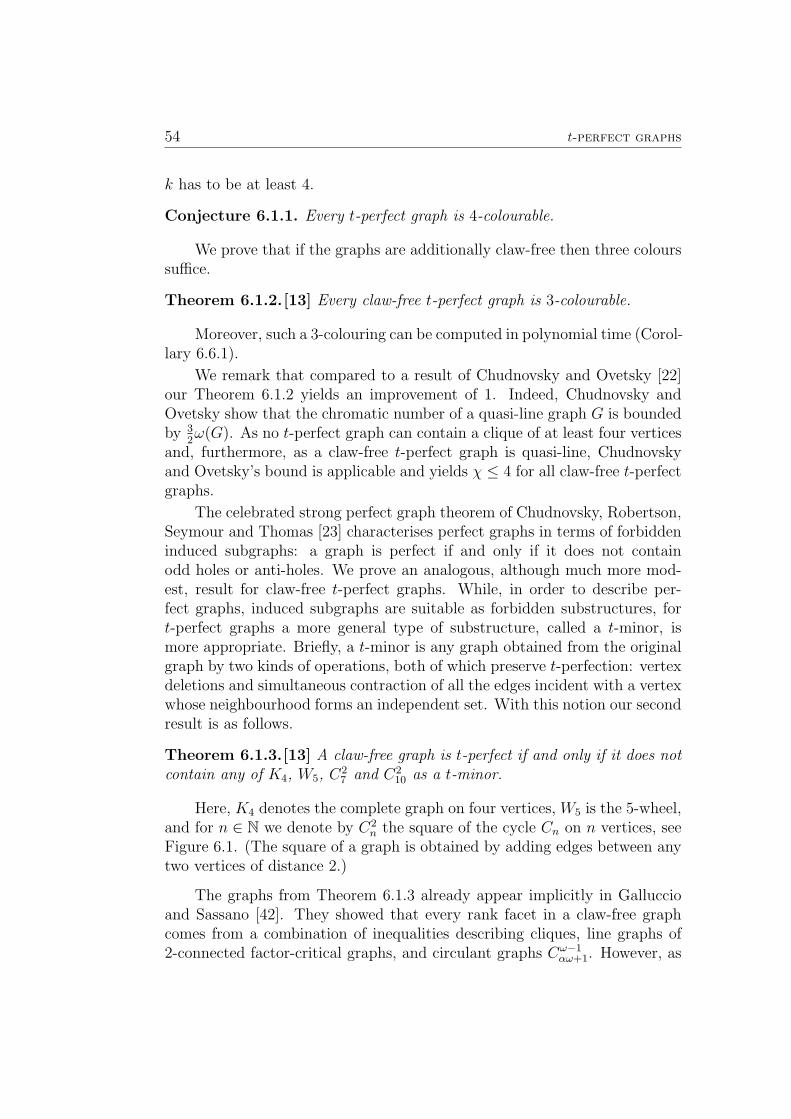
54 t-perfect graphs
k has to be at least 4.
Conjecture 6.1.1. Every t-perfect graph is 4-colourable.
We prove that if the graphs are additionally claw-free then three colourssuffice.
Theorem 6.1.2.[13] Every claw-free t-perfect graph is 3-colourable.
Moreover, such a 3-colouring can be computed in polynomial time (Corol-lary 6.6.1).
We remark that compared to a result of Chudnovsky and Ovetsky [22]our Theorem 6.1.2 yields an improvement of 1. Indeed, Chudnovsky andOvetsky show that the chromatic number of a quasi-line graph G is boundedby 3
2ω(G). As no t-perfect graph can contain a clique of at least four vertices
and, furthermore, as a claw-free t-perfect graph is quasi-line, Chudnovskyand Ovetsky’s bound is applicable and yields χ ≤ 4 for all claw-free t-perfectgraphs.
The celebrated strong perfect graph theorem of Chudnovsky, Robertson,Seymour and Thomas [23] characterises perfect graphs in terms of forbiddeninduced subgraphs: a graph is perfect if and only if it does not containodd holes or anti-holes. We prove an analogous, although much more mod-est, result for claw-free t-perfect graphs. While, in order to describe per-fect graphs, induced subgraphs are suitable as forbidden substructures, fort-perfect graphs a more general type of substructure, called a t-minor, ismore appropriate. Briefly, a t-minor is any graph obtained from the originalgraph by two kinds of operations, both of which preserve t-perfection: vertexdeletions and simultaneous contraction of all the edges incident with a vertexwhose neighbourhood forms an independent set. With this notion our secondresult is as follows.
Theorem 6.1.3.[13] A claw-free graph is t-perfect if and only if it does notcontain any of K4, W5, C2
7 and C210 as a t-minor.
Here, K4 denotes the complete graph on four vertices, W5 is the 5-wheel,and for n ∈ N we denote by C2
n the square of the cycle Cn on n vertices, seeFigure 6.1. (The square of a graph is obtained by adding edges between anytwo vertices of distance 2.)
The graphs from Theorem 6.1.3 already appear implicitly in Galluccioand Sassano [42]. They showed that every rank facet in a claw-free graphcomes from a combination of inequalities describing cliques, line graphs of2-connected factor-critical graphs, and circulant graphs Cω−1
αω+1. However, as
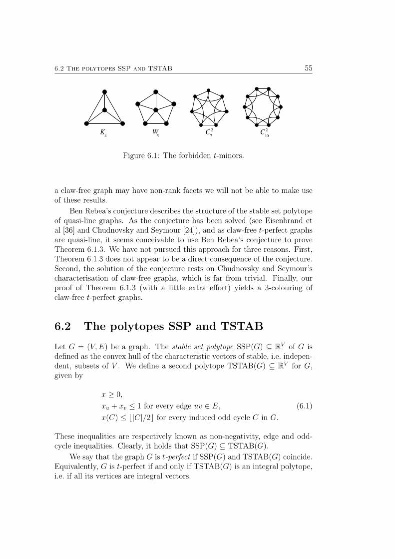
6.2 The polytopes SSP and TSTAB 55
10C 2
7C 2W
5K4
Figure 6.1: The forbidden t-minors.
a claw-free graph may have non-rank facets we will not be able to make useof these results.
Ben Rebea’s conjecture describes the structure of the stable set polytopeof quasi-line graphs. As the conjecture has been solved (see Eisenbrand etal [36] and Chudnovsky and Seymour [24]), and as claw-free t-perfect graphsare quasi-line, it seems conceivable to use Ben Rebea’s conjecture to proveTheorem 6.1.3. We have not pursued this approach for three reasons. First,Theorem 6.1.3 does not appear to be a direct consequence of the conjecture.Second, the solution of the conjecture rests on Chudnovsky and Seymour’scharacterisation of claw-free graphs, which is far from trivial. Finally, ourproof of Theorem 6.1.3 (with a little extra effort) yields a 3-colouring ofclaw-free t-perfect graphs.
6.2 The polytopes SSP and TSTAB
Let G = (V,E) be a graph. The stable set polytope SSP(G) ⊆ RV of G isdefined as the convex hull of the characteristic vectors of stable, i.e. indepen-dent, subsets of V . We define a second polytope TSTAB(G) ⊆ RV for G,given by
x ≥ 0,
xu + xv ≤ 1 for every edge uv ∈ E, (6.1)
x(C) ≤ b|C|/2c for every induced odd cycle C in G.
These inequalities are respectively known as non-negativity, edge and odd-cycle inequalities. Clearly, it holds that SSP(G) ⊆ TSTAB(G).
We say that the graph G is t-perfect if SSP(G) and TSTAB(G) coincide.Equivalently, G is t-perfect if and only if TSTAB(G) is an integral polytope,i.e. if all its vertices are integral vectors.
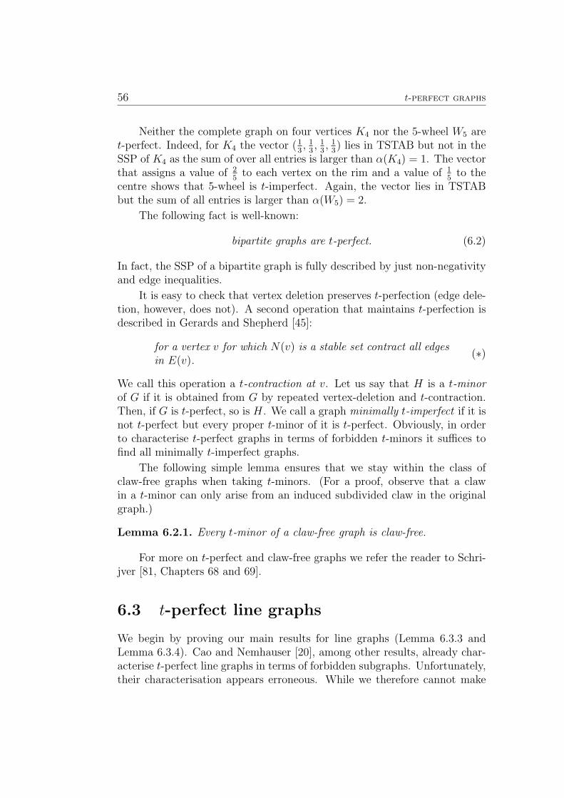
56 t-perfect graphs
Neither the complete graph on four vertices K4 nor the 5-wheel W5 aret-perfect. Indeed, for K4 the vector (1
3, 1
3, 1
3, 1
3) lies in TSTAB but not in the
SSP of K4 as the sum of over all entries is larger than α(K4) = 1. The vectorthat assigns a value of 2
5to each vertex on the rim and a value of 1
5to the
centre shows that 5-wheel is t-imperfect. Again, the vector lies in TSTABbut the sum of all entries is larger than α(W5) = 2.
The following fact is well-known:
bipartite graphs are t-perfect. (6.2)
In fact, the SSP of a bipartite graph is fully described by just non-negativityand edge inequalities.
It is easy to check that vertex deletion preserves t-perfection (edge dele-tion, however, does not). A second operation that maintains t-perfection isdescribed in Gerards and Shepherd [45]:
for a vertex v for which N(v) is a stable set contract all edgesin E(v).
(∗)
We call this operation a t-contraction at v. Let us say that H is a t-minorof G if it is obtained from G by repeated vertex-deletion and t-contraction.Then, if G is t-perfect, so is H. We call a graph minimally t-imperfect if it isnot t-perfect but every proper t-minor of it is t-perfect. Obviously, in orderto characterise t-perfect graphs in terms of forbidden t-minors it suffices tofind all minimally t-imperfect graphs.
The following simple lemma ensures that we stay within the class ofclaw-free graphs when taking t-minors. (For a proof, observe that a clawin a t-minor can only arise from an induced subdivided claw in the originalgraph.)
Lemma 6.2.1. Every t-minor of a claw-free graph is claw-free.
For more on t-perfect and claw-free graphs we refer the reader to Schri-jver [81, Chapters 68 and 69].
6.3 t-perfect line graphs
We begin by proving our main results for line graphs (Lemma 6.3.3 andLemma 6.3.4). Cao and Nemhauser [20], among other results, already char-acterise t-perfect line graphs in terms of forbidden subgraphs. Unfortunately,their characterisation appears erroneous. While we therefore cannot make
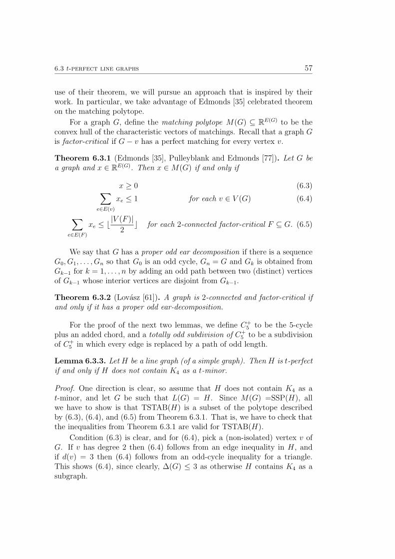
6.3 t-perfect line graphs 57
use of their theorem, we will pursue an approach that is inspired by theirwork. In particular, we take advantage of Edmonds [35] celebrated theoremon the matching polytope.
For a graph G, define the matching polytope M(G) ⊆ RE(G) to be theconvex hull of the characteristic vectors of matchings. Recall that a graph Gis factor-critical if G− v has a perfect matching for every vertex v.
Theorem 6.3.1 (Edmonds [35], Pulleyblank and Edmonds [77]). Let G bea graph and x ∈ RE(G). Then x ∈M(G) if and only if
x ≥ 0 (6.3)∑e∈E(v)
xe ≤ 1 for each v ∈ V (G) (6.4)
∑e∈E(F )
xe ≤ b|V (F )|2c for each 2-connected factor-critical F ⊆ G. (6.5)
We say that G has a proper odd ear decomposition if there is a sequenceG0, G1, . . . , Gn so that G0 is an odd cycle, Gn = G and Gk is obtained fromGk−1 for k = 1, . . . , n by adding an odd path between two (distinct) verticesof Gk−1 whose interior vertices are disjoint from Gk−1.
Theorem 6.3.2 (Lovasz [61]). A graph is 2-connected and factor-critical ifand only if it has a proper odd ear-decomposition.
For the proof of the next two lemmas, we define C+5 to be the 5-cycle
plus an added chord, and a totally odd subdivision of C+5 to be a subdivision
of C+5 in which every edge is replaced by a path of odd length.
Lemma 6.3.3. Let H be a line graph (of a simple graph). Then H is t-perfectif and only if H does not contain K4 as a t-minor.
Proof. One direction is clear, so assume that H does not contain K4 as at-minor, and let G be such that L(G) = H. Since M(G) =SSP(H), allwe have to show is that TSTAB(H) is a subset of the polytope describedby (6.3), (6.4), and (6.5) from Theorem 6.3.1. That is, we have to check thatthe inequalities from Theorem 6.3.1 are valid for TSTAB(H).
Condition (6.3) is clear, and for (6.4), pick a (non-isolated) vertex v ofG. If v has degree 2 then (6.4) follows from an edge inequality in H, andif d(v) = 3 then (6.4) follows from an odd-cycle inequality for a triangle.This shows (6.4), since clearly, ∆(G) ≤ 3 as otherwise H contains K4 as asubgraph.
58 t-perfect graphs
For (6.5), suppose that G contains a 2-connected factor-critical subgraphF , which, by Theorem 6.3.2, has an odd ear-decomposition. So either F isan odd cycle, or F contains a totally odd subdivision X of C+
5 . But in thelatter case, L(X) is an induced subgraph of H, from which we obtain a K4 ast-minor by performing t-contractions at vertices of degree 2, a contradiction.
Hence F is an odd cycle, and (6.5) follows from some odd-cycle inequalityin H. Thus, we have shown that SSP(H) coincides with TSTAB(H), asdesired.
Let G be a claw-free graph with an edge-colouring, and let i, j be twocolours. Denote the subgraph consisting of the edges coloured i or j togetherwith their incident vertices by Gi,j. Note that the components of Gi,j arepaths or cycles.
Lemma 6.3.4. Let H be a t-perfect line graph of a graph. Then χ(H) ≤ 3.
Proof. Let G be a graph such that H = L(G). We do induction on |E(G)|.Pick an edge e = uv. Then clearly, we may apply the induction hypothesisto the t-perfect line graph L(G − e) to deduce that the edges of G − e canbe coloured with three colours.
So, let c be a colouring of the edges of G−e with colours 1, 2, 3. If thereis a colour that is not used by the edges adjacent to e, then we can coloure with that colour and we are done. Thus, assume that all colours 1, 2, 3are used by edges adjacent to e. Since H does not contain K4 as a subgraphwe know that ∆(G) ≤ 3. We may therefore assume that u is incident withtwo edges f1, f2 with c(fi) = i and that v is incident either with one edge g3,or with two edges g1, g3, so that c(gi) = i. We suppose that E(G) cannot becoloured with three colours, which will lead to a contradiction.
Let P ′ be the component of G2,3 containing f2. If g3 does not lie in P ′,then we can swap colours along P ′, such that e is no longer incident withany edge coloured 2, a contradiction. Thus, g3 ∈ E(P ′), and the subpathP := uP ′v has even length. Hence P + e is an odd cycle.
Next, let Q1 be the component of G1,3 containing f1. In fact, Q1 is apath. Suppose Q1 meets P outside u, and let w be the first vertex afteru in Q1 that also lies in P . Then the last edge of Q1w is coloured 1, andQ1w therefore of odd length. We see that (P + e) ∪ Q1w is a totally oddsubdivision of C+
5 , which in H induces K4 as a t-minor, which is impossibleas H is t-perfect. Therefore, V (Q1 ∩ P ) = u.
We swap colours along Q1 and denote the resulting colouring by c′. Notethat c′(f1) = 3 and that P ′ is still coloured with 2, 3. Now, if g1 does notexist, then we can colour e with 1. On the other hand, if g1 exists, then in the
6.4 Squares of cycles 59
same way as before for Q1, we deduce that the component Q2 of G1,2 (withrespect to c′) containing g1 meets P only in v. In particular, by recolouringalong Q2 we obtain a colouring of E(G− e) where no edge incident with e iscoloured with 1, yielding a 3-edge-colouring of G.
The proof of the lemma can easily be turned into an algorithm withrunning time O(n3), where n is the number of vertices. (We are cheatinghere a bit. The proof supposes that we know the graph G of which H is theline graph. However, with minor complications, the same induction can beperformed directly in H.)
Corollary 6.3.5. A t-perfect line graph can be coloured with three coloursin polynomial time.
6.4 Squares of cycles
As a preparation for our main lemma we show in this section that mostsquares of cycles are t-imperfect. In fact, the only t-perfect squares of cyclesare C2
3 , which is a triangle, and C26 , the line graph of K4.
Recall that C2n denotes the square of a cycle of order n. We shall always
assume that V (C2n) = v1, . . . , vn where the vertices are labelled in cyclic
order.
Lemma 6.4.1. Let n ≥ 4, and let n /∈ 6, 7, 10. Then K4 is a t-minor ofC2n. Moreover, for n ≥ 8 the K4-t-minor is already contained in C2
n − v5.
Proof. Since C24 = K4 we only need to concern ourselves with C2
n for n ≥ 5.Depending on n mod 4 we perform vertex-deletions and then t-contractionsas indicated in Figure 6.2 until the only vertices left are v1, . . . , v4. In partic-ular, we delete the grey vertices in the initial segment (marked by a dashedbox). Outside this segment we delete every other vertex until we reach thefirst vertex v1 again. Finally, we contract the odd path between v4 and v1 toa single edge.
The length of the initial segment poses a constraint on the minimal sizeof the graph. For n ≡ 0 (mod 4) the construction is possible for n ≥ 8, forn ≡ 1 we need n ≥ 5, for n ≡ 2 we need n ≥ 14, and n ≥ 11 is necessary forn ≡ 3. So the only cases we have not dealt with are n = 6, 7, 10, which areprecisely the exceptions. The second part of the assertion follows directlyfrom the construction of the subdivision of K4.
Lemma 6.4.2. No square of a cycle of length at least 7 is t-perfect.
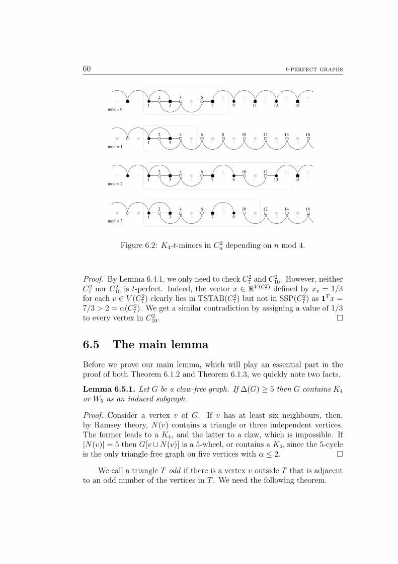
60 t-perfect graphs
3
42 6
7 9 11 13 15
161412108
5
3
42 6 8 10 12 14 16
5 7 9 11 13 15
3
42 6
7 9
10 12
13 155
8
11
14 16
3
42 6
7 9
10 12 14 16
5
8
11 13 151
1
1
1mod = 0
mod = 1
mod = 2
mod = 3
Figure 6.2: K4-t-minors in C2n depending on n mod 4.
Proof. By Lemma 6.4.1, we only need to check C27 and C2
10. However, neitherC2
7 nor C210 is t-perfect. Indeed, the vector x ∈ RV (C2
7 ) defined by xv = 1/3for each v ∈ V (C2
7) clearly lies in TSTAB(C27) but not in SSP(C2
7) as 1Tx =7/3 > 2 = α(C2
7). We get a similar contradiction by assigning a value of 1/3to every vertex in C2
10.
6.5 The main lemma
Before we prove our main lemma, which will play an essential part in theproof of both Theorem 6.1.2 and Theorem 6.1.3, we quickly note two facts.
Lemma 6.5.1. Let G be a claw-free graph. If ∆(G) ≥ 5 then G contains K4
or W5 as an induced subgraph.
Proof. Consider a vertex v of G. If v has at least six neighbours, then,by Ramsey theory, N(v) contains a triangle or three independent vertices.The former leads to a K4, and the latter to a claw, which is impossible. If|N(v)| = 5 then G[v ∪N(v)] is a 5-wheel, or contains a K4, since the 5-cycleis the only triangle-free graph on five vertices with α ≤ 2.
We call a triangle T odd if there is a vertex v outside T that is adjacentto an odd number of the vertices in T . We need the following theorem.
6.5 The main lemma 61
Theorem 6.5.2 (Harary [53, Theorem 8.4]). Let G be a claw-free graph.Then G is a line graph if and only if every pair of odd triangles that sharesexactly one edge induces a K4.
Let us now state the main lemma. It shows that the structure of a claw-free t-perfect graph is rather restricted, provided the graph is 3-connected.
Lemma 6.5.3 (Main lemma). Let G be a 3-connected claw-free graph with∆(G) ≤ 4. If G does not contain K4 as t-minor then one of the followingstatements holds true:
(i) G is a line graph;
(ii) G ∈ C26 − v1v6, C
27 − v7, C
210 − v10, C
27 , C
210.
Proof. We shall repeatedly make use of the following argument. Assume thatin the neighbourhood of a vertex u we find a path xyz, and assume that uhas a fourth neighbour v /∈ x, y, z. As K4 is not a subgraph of G we knowthat xz /∈ E(G). Then, because G is claw-free, v has to be adjacent to x orto z or to both.
First of all, we shall show that
P 26 is a subgraph of G. (6.6)
Recall that Pk denotes a path on k vertices.
Indeed, as we may assume that G is not a line graph, there exist byTheorem 6.5.2 two odd triangles that share exactly one edge, say u1u2u3 andu2u3u4. As G is 3-connected, u1, u4 does not separate G, and thus oneof u2 and u3 has a neighbour u5 /∈ u1, u2, u3, u4. By symmetry, we mayassume that u3u5 ∈ E(G) and by the argument outlined at the beginning ofthis proof, we deduce from u1u2u4 ⊆ G[N(u3)] that u5 is adjacent to u1 orto u4 (or to both). Symmetry, again, allows us to assume that u5 is adjacentto u4.
As K4 is not a subgraph of G, u1 and u5 each send exactly two edgesto the triangle u2u3u4. That triangle, however, is odd. Thus there existsa vertex u6 /∈ u1, . . . , u5 that is adjacent to an odd number of vertices ofthe triangle. Since u3 has four neighbours already among the ui, it followsthat u6 is either adjacent to u2 or to u4. By forgetting that u1u2u3 is odd,we obtain again a symmetric graph on u1, . . . , u5, which means that we may,without loss of generality, assume that u6u4 ∈ E(G), and that u6u2 /∈ E(G).The path u2u3u5 that is contained in the neighbourhood of u4 together withu6u2 /∈ E(G) ensures that u6 is adjacent to u5. This proves (6.6).
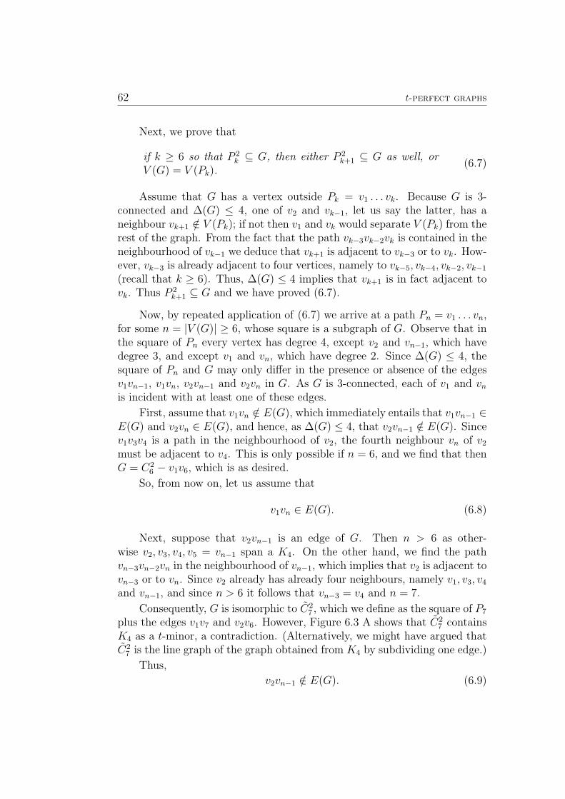
62 t-perfect graphs
Next, we prove that
if k ≥ 6 so that P 2k ⊆ G, then either P 2
k+1 ⊆ G as well, orV (G) = V (Pk).
(6.7)
Assume that G has a vertex outside Pk = v1 . . . vk. Because G is 3-connected and ∆(G) ≤ 4, one of v2 and vk−1, let us say the latter, has aneighbour vk+1 /∈ V (Pk); if not then v1 and vk would separate V (Pk) from therest of the graph. From the fact that the path vk−3vk−2vk is contained in theneighbourhood of vk−1 we deduce that vk+1 is adjacent to vk−3 or to vk. How-ever, vk−3 is already adjacent to four vertices, namely to vk−5, vk−4, vk−2, vk−1
(recall that k ≥ 6). Thus, ∆(G) ≤ 4 implies that vk+1 is in fact adjacent tovk. Thus P 2
k+1 ⊆ G and we have proved (6.7).
Now, by repeated application of (6.7) we arrive at a path Pn = v1 . . . vn,for some n = |V (G)| ≥ 6, whose square is a subgraph of G. Observe that inthe square of Pn every vertex has degree 4, except v2 and vn−1, which havedegree 3, and except v1 and vn, which have degree 2. Since ∆(G) ≤ 4, thesquare of Pn and G may only differ in the presence or absence of the edgesv1vn−1, v1vn, v2vn−1 and v2vn in G. As G is 3-connected, each of v1 and vnis incident with at least one of these edges.
First, assume that v1vn /∈ E(G), which immediately entails that v1vn−1 ∈E(G) and v2vn ∈ E(G), and hence, as ∆(G) ≤ 4, that v2vn−1 /∈ E(G). Sincev1v3v4 is a path in the neighbourhood of v2, the fourth neighbour vn of v2
must be adjacent to v4. This is only possible if n = 6, and we find that thenG = C2
6 − v1v6, which is as desired.
So, from now on, let us assume that
v1vn ∈ E(G). (6.8)
Next, suppose that v2vn−1 is an edge of G. Then n > 6 as other-wise v2, v3, v4, v5 = vn−1 span a K4. On the other hand, we find the pathvn−3vn−2vn in the neighbourhood of vn−1, which implies that v2 is adjacent tovn−3 or to vn. Since v2 already has already four neighbours, namely v1, v3, v4
and vn−1, and since n > 6 it follows that vn−3 = v4 and n = 7.
Consequently, G is isomorphic to C27 , which we define as the square of P7
plus the edges v1v7 and v2v6. However, Figure 6.3 A shows that C27 contains
K4 as a t-minor, a contradiction. (Alternatively, we might have argued thatC2
7 is the line graph of the graph obtained from K4 by subdividing one edge.)
Thus,
v2vn−1 /∈ E(G). (6.9)
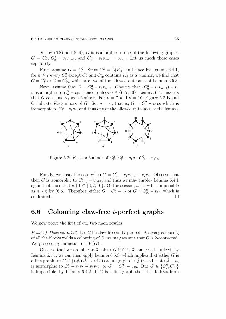
6.6 Colouring claw-free t-perfect graphs 63
So, by (6.8) and (6.9), G is isomorphic to one of the following graphs:G = C2
n, C2n − v1vn−1, and C2
n − v1vn−1 − v2vn. Let us check these casesseperately.
First, assume G = C2n. Since C2
6 = L(K4) and since by Lemma 6.4.1,for n ≥ 7 every C2
n except C27 and C2
10 contains K4 as a t-minor, we find thatG = C2
7 or G = C210, which are two of the allowed outcomes of Lemma 6.5.3.
Next, assume that G = C2n − v1vn−1. Observe that (C2
n − v1vn−1) − v1
is isomorphic to C2n − v5. Hence, unless n ∈ 6, 7, 10, Lemma 6.4.1 asserts
that G contains K4 as a t-minor. For n = 7 and n = 10, Figure 6.3 B andC indicate K4-t-minors of G. So, n = 6, that is, G = C2
6 − v1v5 which isisomorphic to C2
6 −v1v6, and thus one of the allowed outcomes of the lemma.
1
2
456
7
9
10
38
2
4
7
36
5
1
A
2
4
7
36
5
1
B C
Figure 6.3: K4 as a t-minor of C27 , C2
7 − v1v6, C210 − v1v9.
Finally, we treat the case when G = C2n − v1vn−1 − v2vn. Observe that
then G is isomorphic to C2n+1 − vn+1, and thus we may employ Lemma 6.4.1
again to deduce that n+1 ∈ 6, 7, 10. Of these cases, n+1 = 6 is impossibleas n ≥ 6 by (6.6). Therefore, either G = C2
7 − v7 or G = C210 − v10, which is
as desired.
6.6 Colouring claw-free t-perfect graphs
We now prove the first of our two main results.
Proof of Theorem 6.1.2. Let G be claw-free and t-perfect. As every colouringof all the blocks yields a colouring of G, we may assume that G is 2-connected.We proceed by induction on |V (G)|.
Observe that we are able to 3-colour G if G is 3-connected. Indeed, byLemma 6.5.1, we can then apply Lemma 6.5.3, which implies that either G isa line graph, or G ∈ C2
7 , C210 or G is a subgraph of C2
6 (recall that C27 − v5
is isomorphic to C26 − v1v5 − v2v6), or G = C2
10 − v10. But G ∈ C27 , C
210
is impossible, by Lemma 6.4.2. If G is a line graph then it it follows from
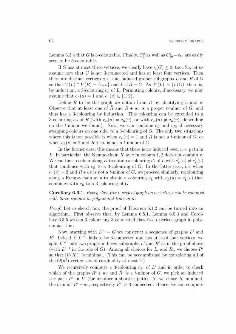
64 t-perfect graphs
Lemma 6.3.4 that G is 3-colourable. Finally, C26 as well as C2
10−v10 are easilyseen to be 3-colourable.
If G has at most three vertices, we clearly have χ(G) ≤ 3, too. So, let usassume now that G is not 3-connected and has at least four vertices. Thenthere are distinct vertices u, v, and induced proper subgraphs L and R of Gso that V (L) ∩ V (R) = u, v and L ∪R = G. As |V (L)| < |V (G)| there is,by induction, a 3-colouring cL of L. Permuting colours, if necessary, we mayassume that cL(u) = 1 and cL(v) ∈ 1, 2.
Define R to be the graph we obtain from R by identifying u and v.Observe that at least one of R and R + uv is a proper t-minor of G, andthus has a 3-colouring by induction. This colouring can be extended to a3-colouring cR of R (with cR(u) = cR(v), or with cR(u) 6= cR(v), dependingon the t-minor we found). Now, we can combine cL and cR, if necessaryswapping colours on one side, to a 3-colouring of G. The only two situationswhere this is not possible is when cL(v) = 1 and R is not a t-minor of G, orwhen cL(v) = 2 and R + uv is not a t-minor of G.
In the former case, this means that there is no induced even u–v path inL. In particular, the Kempe-chain K at u in colours 1, 2 does not contain v.We can thus recolour alongK to obtain a colouring c′L of L with c′L(u) 6= c′L(v)that combines with cR to a 3-colouring of G. In the latter case, i.e. whencL(v) = 2 and R+uv is not a t-minor of G, we proceed similarly, recolouringalong a Kempe-chain at u to obtain a colouring c′L with c′L(u) = c′L(v) thatcombines with cR to a 3-colouring of G
Corollary 6.6.1. Every claw-free t-perfect graph on n vertices can be colouredwith three colours in polynomial time in n.
Proof. Let us sketch how the proof of Theorem 6.1.2 can be turned into analgorithm. First observe that, by Lemma 6.5.1, Lemma 6.5.3 and Corol-lary 6.3.5 we can 3-colour any 3-connected claw-free t-perfect graph in poly-nomial time.
Now, starting with L0 := G we construct a sequence of graphs Li andRi. Indeed, if Li−1 fails to be 3-connected and has at least four vertices, wesplit Li−1 into two proper induced subgraphs Li and Ri as in the proof above(with Li−1 in the role of G). Among all choices for Li and Ri, we choose Ri
so that |V (Ri)| is minimal. (This can be accomplished by considering all ofthe O(n2) vertex sets of cardinality at most 2.)
We recursively compute a 3-colouring cLi of Li and in order to checkwhich of the graphs Ri + uv and Ri is a t-minor of G, we pick an inducedu-v path P i in Li (for instance a shortest path). As we chose Ri minimal,the t-minor Ri +uv, respectively Ri, is 3-connected. Hence, we can compute

6.6 Colouring claw-free t-perfect graphs 65
its 3-colouring directly with the help of Lemma 6.5.3 and Corollary 6.3.5. Ifnecessary, we then recolour Li along a Kempe-chain at u. Since Li−1−Li 6= ∅,the procedure stops after at most n steps.
Let us now turn for a moment to h-perfect graphs, to which our resulton colourings easily carries over. Sbihi and Uhry [79] introduced h-perfectgraphs as a common generalisation of perfect and t-perfect graphs. For thedefinition of h-perfect graphs we use the same inequalities as for t-perfectgraphs, only that the edge inequalities are replaced with clique inequalities.So, a graph is called h-perfect if the SSP is determined by
x ≥ 0
x(K) ≤ 1 for every clique K
x(C) ≤ b|V (C)|/2c for every induced odd cycle C
The proof of the following corollary is due to Sebo [72]. As it has notbeen published but contains a nice and useful technique we present it here.
Corollary 6.6.2. Let G be a claw-free h-perfect graph. Then
(i) χ(G) = dχ∗(G)e; and
(ii) χ(G) = ω(G) if ω(G) ≥ 3.
Here, χ∗ denotes the fractional chromatic number. More formally, if Sdenotes the set of all stable sets:
χ∗(G) = min 1Ty, y ∈ RS
subject to y ≥ 0 and∑
S∈S, v∈S
yS ≥ 1 for all v ∈ V (6.10)
Proof of Corollary 6.6.2. Define the polytope
P = x ∈ RV : x(S) ≤ 1 for each stable set S, x ≥ 0.
Observe that maxx∈P 1Tx is the dual program of (6.10), so that we getχ∗(G) = maxx∈P 1Tx. Moreover, it is not hard to check that the anti-blockingpolytope of P coincides with SSP(G). As G is h-perfect, Theorem 2.1 in Fulk-erson [41] (see also [40]) yields therefore that every vertex 6= 0 of P is eitherthe characteristic vector χK of a clique K of G or the vertex is of the form
2|C|−1
χC for an odd cycle C.
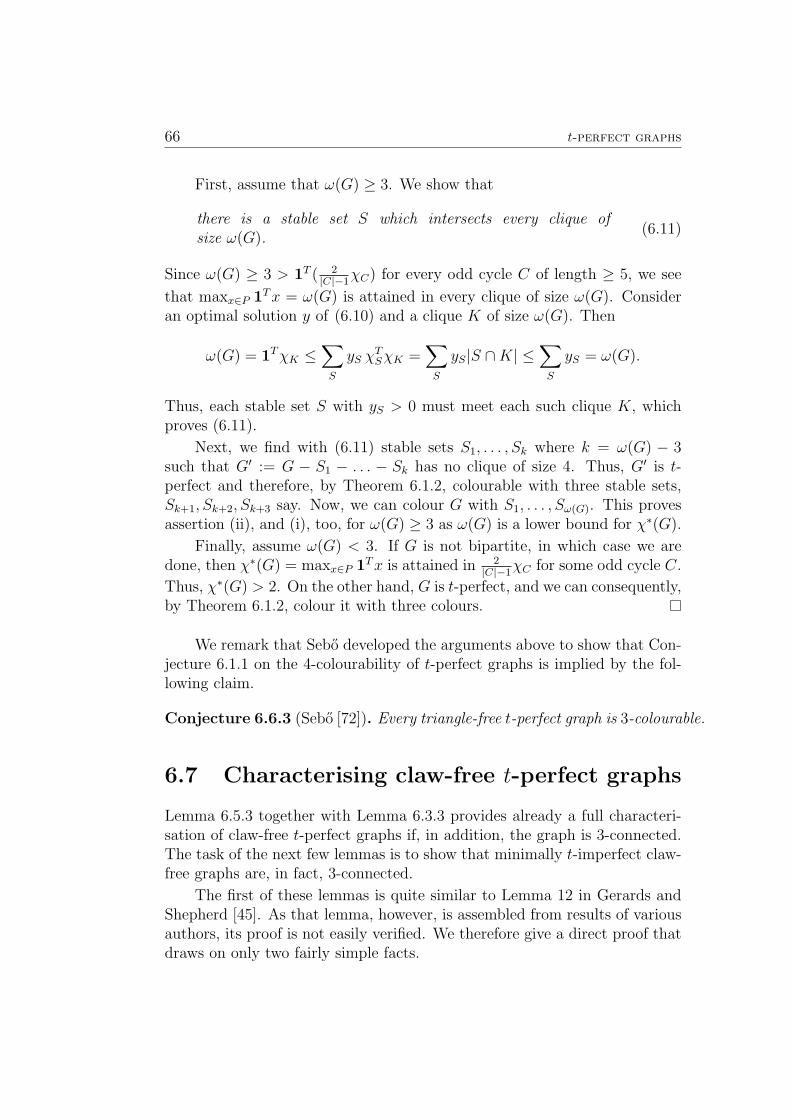
66 t-perfect graphs
First, assume that ω(G) ≥ 3. We show that
there is a stable set S which intersects every clique ofsize ω(G).
(6.11)
Since ω(G) ≥ 3 > 1T ( 2|C|−1
χC) for every odd cycle C of length ≥ 5, we see
that maxx∈P 1Tx = ω(G) is attained in every clique of size ω(G). Consideran optimal solution y of (6.10) and a clique K of size ω(G). Then
ω(G) = 1TχK ≤∑S
yS χTSχK =
∑S
yS|S ∩K| ≤∑S
yS = ω(G).
Thus, each stable set S with yS > 0 must meet each such clique K, whichproves (6.11).
Next, we find with (6.11) stable sets S1, . . . , Sk where k = ω(G) − 3such that G′ := G − S1 − . . . − Sk has no clique of size 4. Thus, G′ is t-perfect and therefore, by Theorem 6.1.2, colourable with three stable sets,Sk+1, Sk+2, Sk+3 say. Now, we can colour G with S1, . . . , Sω(G). This provesassertion (ii), and (i), too, for ω(G) ≥ 3 as ω(G) is a lower bound for χ∗(G).
Finally, assume ω(G) < 3. If G is not bipartite, in which case we aredone, then χ∗(G) = maxx∈P 1Tx is attained in 2
|C|−1χC for some odd cycle C.
Thus, χ∗(G) > 2. On the other hand, G is t-perfect, and we can consequently,by Theorem 6.1.2, colour it with three colours.
We remark that Sebo developed the arguments above to show that Con-jecture 6.1.1 on the 4-colourability of t-perfect graphs is implied by the fol-lowing claim.
Conjecture 6.6.3 (Sebo [72]). Every triangle-free t-perfect graph is 3-colourable.
6.7 Characterising claw-free t-perfect graphs
Lemma 6.5.3 together with Lemma 6.3.3 provides already a full characteri-sation of claw-free t-perfect graphs if, in addition, the graph is 3-connected.The task of the next few lemmas is to show that minimally t-imperfect claw-free graphs are, in fact, 3-connected.
The first of these lemmas is quite similar to Lemma 12 in Gerards andShepherd [45]. As that lemma, however, is assembled from results of variousauthors, its proof is not easily verified. We therefore give a direct proof thatdraws on only two fairly simple facts.
6.7 Characterising claw-free t-perfect graphs 67
Lemma 6.7.1. Let G be a minimally t-imperfect graph, and assume u, v ∈V (G) to separate G. Then G − u, v has exactly two components, one ofwhich is a (possibly trivial) path. Moreover, uv /∈ E(G).
Proof. Let G = G1∪G2 so that u, v separates G1−u, v from G2−u, v.Suppose that neither of G1 and G2 is a path. Let z be a non-integral vertex ofTSTAB(G), denote by I the set of those non-negativity, edge and odd-cycleinequalities that are satisfied with equality by z. We define z1 resp. z2 to bethe restriction of z to G1 resp. G2.
As in the proof of Theorem 1 in Gerards and Shepherd [45] we candeduce that
0 < zw < 1 for all w ∈ V (G) (6.12)
and
every odd cycle whose inequality is in I fails to separate G. (6.13)
The last fact implies, in particular, that each odd cycle in I lies eithercompletely in G1 or in G2 (recall that neither of G1 and G2 is a path).Thus, we can partition I in (I1, I2) so that Ik pertains only to Gk. Now,if there is a j ∈ 1, 2 so that dim Ij = |V (Gj)| then zj is a vertex ofTSTAB(Gj) =SSP(Gj). Since zj is non-integral we obtain a contradiction.
Therefore, we have dim Ik = |V (Gk)| − 1 for k = 1, 2, which meansthat Ik describes an edge of TSTAB(Gk). Denote the endvertices of thisedge by sk and tk, i.e. zk = λks
k + (1 − λk)tk for some 0 ≤ λk ≤ 1. As
TSTAB(Gk) =SSP(Gk) by assumption, it follows that sk is the characteristicvector of a stable set Sk of Gk; the same holds for tk and a stable set Tk.
By (6.12), z1u = z2
u > 0 and thus for each k = 1, 2 one of Sk and Tk needsto contain u. By renaming if necessary we may assume that u ∈ S1 andu ∈ S2. Then u /∈ Tk for k = 1, 2 as otherwise we obtain zku = λk+(1−λk) = 1in contradiction to (6.12). This implies that
λ1 = z1u = zu = z2
u = λ2. (6.14)
If S1∩v = S2∩v then also T1∩v = T2∩v as (6.12) implies as abovethat v ∈ Sk if and only if v /∈ Tk. In this case, S := S1 ∪S2 and T := T1 ∪ T2
are stable sets of G and we obtain z = λ1χS + (1− λ1)χT , contradicting thechoice of z as a non-integral vertex of TSTAB(G).
So, let us assume that S1 and S2 differ on v. Without loss of generality,let v ∈ S1 but v /∈ S2. Then
S1 ∩ u, v = u, v, T1 ∩ u, v = ∅,S2 ∩ u, v = u and T2 ∩ u, v = v.
68 t-perfect graphs
So, λ1 = z1v = z2
v = 1−λ2, and hence, by (6.14), λ1 = λ2 = 1/2. In particular,it follows with (6.12) again that zw = 1/2 for all w ∈ V (G).
Now, since bipartite graphs are t-perfect by (6.2), G contains an oddcycle of length 2k + 1, say. However, adding up z along the cycle yieldsk + 1/2, contradicting the odd-cycle inequalities.
Next, let us prove that a minimally t-imperfect claw-free graph has min-imum degree at least three. We start with a lemma that is a variant ofTheorem 2.5 in Barahona and Mahjoub [2], and can be proved in a verysimilar way
Lemma 6.7.2 (Barahona and Mahjoub [2]). Let G be a graph, and let uvwbe a path in G so that deg(v) = 2 and uw /∈ E(G). Furthermore, let aTx ≤ αbe a facet-defining inequality of SSP(G) so that au = av = aw. Denote byG′ the graph obtained from G by contracting uv and vw, and let v be theresulting vertex, i.e. V (G′)\V (G) = v. If a′ ∈ RV (G′) is defined by a′p = apfor p ∈ V (G′−v) and av = av then a′Tx ≤ α−av is a facet-defining inequalityof SSP(G′).
The following lemma serves to guarantee that au = av = aw as inLemma 6.7.2.
Lemma 6.7.3. Let G be a graph and assume that for a ∈ RV (G), a > 0 theinequality aTx ≤ α is facet-defining in SSP(G), and that it is not a multipleof an edge inequality or of an odd-cycle inequality.
(i) If G contains a path uvw so that deg(v) = 2 then av ≤ aw.
(ii) If G contains a triangle wpq and a neighbour v /∈ p, q of w so thatdeg(w) = 3 then av ≥ aw.
Assertion (i) appears in Mahjoub [71].
Proof. For both cases, observe that as the SSP is full-dimensional there existsa set S of |V (G)| affinely independent stable sets that satisfy aTx ≤ α withequality. Since a > 0 it follows that α 6= 0, which, in turn, implies that thecharacteristic vectors of the stable sets in S are even linearly independent.In particular, any inequality satisfied with equality by all S ∈ S is a multipleof aTx ≤ α.
(i) Since aTx ≤ α is not a multiple of the edge inequality xu + xv ≤ 1there must exist an S0 ∈ S so that u /∈ S0 and v /∈ S0. As a > 0 thisimplies that w ∈ S0. Clearly, S ′0 := S0 \ w ∪ v is a stable set and thusaTχS′0 ≤ α = aTχS0 . Hence av ≤ aw.
6.7 Characterising claw-free t-perfect graphs 69
(ii) Since aTx ≤ α is not a multiple of the triangle inequality xw + xp +xq ≤ 1 there must exist an S1 ∈ S so that w, p, q ∩S1 = ∅. Then, as a > 0and N(w) = v, p, q, we have that v ∈ S1 and that S ′1 := S1 \ v ∪ w isstable. Again, we obtain aTχS′1 ≤ α = aTχS1 and therefore aw ≤ av.
Lemma 6.7.4. Let G be a minimally t-imperfect claw-free graph. Then Ghas minimum degree ≥ 3.
Proof. It is easy to see that no vertex can have degree 1. Indeed, such avertex would lead to a violation as in (6.12). So suppose there is a pathP = w1 . . . wk with k ≥ 3 so that all internal vertices have degree 2 in Gbut w1 and wk have degree > 2. Since G is claw-free and does not properlycontain a K4 we deduce that deg(w1) = deg(wk) = 3, and in fact thereare neighbours p1, q1 of w1 and pk, qk of wk so that w1p1q1 and wkpkqk aretriangles in G.
As G is t-imperfect there exists a facet-defining inequality aTx ≤ α ofSSP(G) with a ≥ 0 that is not a multiple of a non-negativity, edge or odd-cycle inequality. Since G is minimally t-imperfect under vertex deletion itfollows furthermore that a > 0.
Now, applying (i) of Lemma 6.7.3 we get that aw2 = . . . = awk−1≤
minw1, wk. Then, (ii) yields that aw1 = aw2 = . . . = awk.
Denote by G′ the graph obtained from G by performing a t-contractionat w2, and let w be the resulting new vertex. Define a′u = au for u ∈ V (G′−w)and a′w = aw2 . Then, by Lemma 6.7.2, a′Tx ≤ α − aw2 is facet-defining forSSP(G′). However, as a′ > 0 and as G′ is t-perfect it follows that G′ consistsof a single vertex, a single edge or of a single odd cycle. Then G is such agraph, too, and thus t-perfect, a contradiction.
In Section 6.8 we will show in Lemma 6.8.1 that C27 − v7 as well as
C210 − v10 are (strongly t-perfect and thus) t-perfect. Considering Figure 6.4
we see that C26−v1v6 is a t-minor of C2
10−v10. Hence, (assuming Lemma 6.8.1)the following lemma holds:
Lemma 6.7.5. C27 − v7, C2
10 − v10 and C26 − v1v6 are t-perfect.
We now prove our second main result.
Proof of Theorem 6.1.3. As neither of K4,W5, C27 and C2
10 is t-perfect (noteLemma 6.4.2), necessity is obvious. To prove sufficiency, consider a claw-freeand minimally t-imperfect graph G.
Lemmas 6.7.1 and 6.7.4 ensure that G is 3-connected. Moreover, as weare done if G contains K4 or W5 as a t-minor, we obtain with Lemma 6.5.1

70 t-perfect graphs
6~ 6~
2
3
4
5
1
6
10
9
8
7
1
2
3
4
5
=2
3
4
5
1
Figure 6.4: C26 − v1v6 is a t-minor of C2
10 − v10.
that ∆(G) ≤ 4. Consequently, all preconditions of Lemma 6.5.3 are satisfied,and we may assume that G is of type (i) or (ii) as listed in Lemma 6.5.3.
Now, if G is a line graph then Lemma 6.3.3 forces G to contain K4 asa t-minor, as desired. It remains to check the types listed in (ii). As byLemma 6.7.5, the graphs C2
6 − v1v6, C27 − v7 and C2
10 − v10 are t-perfect, itfollows that G ∈ C2
7 , C210, as desired.
6.8 C27 and C2
10 are minimally t-imperfect
To conclude the proof of Theorem 6.1.3 it still remains to prove one lastlemma (since we needed for the proof of Lemma 6.7.5 that C2
7 − v7 andC2
10−v10 are t-perfect). We take this opportunity to show something slightlystronger, namely that C2
7 and C210 are minimally t-imperfect, and, moreover,
minimally strongly t-imperfect.
In order to define strong t-perfection, consider a graph G and w ∈ ZV (G),and denote by αw(G) the maximum w(S) over all stable sets S in G. Call afamily K of edges and odd cycles a w-cover of G if every vertex v lies in atleast w(v) members of K. If K consists of the subfamily of edges E and thesubfamily of cycles C then it has cost
|E|+∑C∈C
|C| − 1
2.
We say that G is strongly t-perfect if for every w ∈ ZV (G) there is a w-coverof cost at most αw(G). (Clearly, any w-cover has cost at least αw(G).) Thisis equivalent to defining strongly t-perfect graphs as those for which (6.1) istotally dual integral.
Observe that it suffices to check the existence of the desired cover for allnon-negative vectors w. Moreover, one can show that vertex deletion as wellas t-contraction maintain strong t-perfection.
6.8 C27 and C2
10 are minimally t-imperfect 71
Strongly t-perfect graphs have been studied by Gerards [44] and Schrij-ver [80]; see also Schrijver [81, Chapter 68]. They show that bad resp. oddK4-free graphs are strongly t-perfect. It is not known whether a t-perfectgraph is necessarily strongly t-perfect, but the converse is true. So, the t-perfectness of C2
7 − v7 and C210 − v10 follows from the following lemma.
Lemma 6.8.1. For j ∈ 7, 10, the graph C2j − vj is strongly t-perfect.
The proof of this lemma is a bit involved and given below. Let us firstget to the main result of this section:
Proposition 6.8.2. [13] The graphs C27 and C2
10 are minimally t-imperfectas well as minimally strongly-t-imperfect.
Proof. Lemma 6.4.2 yields that C27 and C2
10 are t-imperfect, and by Lemma 6.8.1,we know that the deletion of one vertex makes these graphs strongly t-perfect.Hence, as strong t-perfection implies t-perfection, our proposition follows.
Proof of Lemma 6.8.1. In both cases, j = 7 and j = 10, we proceed byinduction on the total weight w(V ), where V := V (C2
j − vj) and w is thegiven non-negative vector in ZV for which we have to find a w-cover. So,let G ∈ C2
7 − v7, C210 − v10. As the case when w(V ) = 0 is trivial we will
assume that w is given with w(V ) > 0, and that the desired cover exists forall w′ with w′(V ) < w(V ).
Let v1, . . . , vj−1 be the vertices of V (G) in circular order, so thatv1, v2, vj−2 and vj−1 have degree 3. Denote by S the set of all stable setsof weight αw := αw(G), and write wi for w(vi).
First of all, if there is triangle T so that every S ∈ S meets T , then wedefine w′(v) := w(v)−1 for v ∈ T+ := V (T )∩⋃S∈S S and w′i = wi otherwise.As each v ∈ T+ has positive weight w(v)—otherwise S\v would be in S andmiss T—we conclude that w′ is non-negative. Since T+ 6= ∅ by assumption,the total weight w′(V ) is smaller than w(V ). Hence, by induction there is aw′-cover K′ of cost αw′ . Since αw′ = αw − 1 the family K′ ∪ T is a w-cover ofcost αw, as desired.
We can argue similarly if every S ∈ S meets the edge v1vj−1. So, letus assume from now on that for each triangle T in G there is a ST ∈ Savoiding T , and that there exists a Sv1vj
that is disjoint from v1, vj−1.In the case when G = C2
7 − v7, the stable set Sv4v5v6 of weight αw needsto consist of a single vertex vk with k ∈ 1, 2, 3 as v1v2v3 forms a trianglein G. Hence, wk = αw. In the same way, we get that for some l ∈ 4, 5, 6the vertex vl has weight αw, too. Moreover, vk and vl have to be adjacent.If (k, l) = (1, 6), then all other vertices have weight 0, and αw times the edge
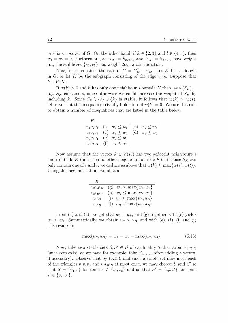
72 t-perfect graphs
v1v6 is a w-cover of G. On the other hand, if k ∈ 2, 3 and l ∈ 4, 5, thenw1 = w6 = 0. Furthermore, as v2 = Sv3v4v5 and v5 = Sv2v3v4 have weightαw, the stable set v2, v5 has weight 2αw, a contradiction.
Now, let us consider the case of G = C210 − v10. Let K be a triangle
in G, or let K be the subgraph consisting of the edge v1v9. Suppose thatk ∈ V (K).
If w(k) > 0 and k has only one neighbour s outside K then, as w(SK) =αw, SK contains s, since otherwise we could increase the weight of SK byincluding k. Since SK \ s ∪ k is stable, it follows that w(k) ≤ w(s).Observe that this inequality trivially holds too, if w(k) = 0. We use this ruleto obtain a number of inequalities that are listed in the table below.
Kv1v2v3 (a) w1 ≤ w9 (b) w2 ≤ w4
v7v8v9 (c) w9 ≤ w1 (d) w8 ≤ w6
v2v3v4 (e) w2 ≤ w1
v6v7v8 (f) w8 ≤ w9
Now assume that the vertex k ∈ V (K) has two adjacent neighbours sand t outside K (and then no other neighbours outside K). Because SK canonly contain one of s and t, we deduce as above that w(k) ≤ maxw(s), w(t).Using this argumentation, we obtain
Kv3v4v5 (g) w3 ≤ maxw1, w2v5v6v7 (h) w7 ≤ maxw8, w9v1v9 (i) w1 ≤ maxw2, w3v1v9 (j) w9 ≤ maxw7, w8
From (a) and (c), we get that w1 = w9, and (g) together with (e) yieldsw3 ≤ w1. Symmetrically, we obtain w7 ≤ w9, and with (e), (f), (i) and (j)this results in
maxw2, w3 = w1 = w9 = maxw7, w8. (6.15)
Now, take two stable sets S, S ′ ∈ S of cardinality 2 that avoid v4v5v6
(such sets exist, as we may, for example, take Sv4v5v6 , after adding a vertex,if necessary). Observe that by (6.15), and since a stable set may meet eachof the triangles v1v2v3 and v7v8v9 at most once, we may choose S and S ′ sothat S = v1, s for some s ∈ v7, v8 and so that S ′ = v9, s
′ for somes′ ∈ v2, v3.
6.8 C27 and C2
10 are minimally t-imperfect 73
Comparing the stable set v1, s, v4 to S we get w1+w(s)+w4 ≤ w(S) =w1+w(s) and thus w4 = 0. Hence, w2 = 0 too, by (b), and w3 = w1, by (6.15).Symmetrically, comparing v9, s
′, v6 to S ′, we get that w6 = w8 = 0.
To sum up, we have discovered that w1 = w3 = w7 = w9 and thatw2 = w4 = w6 = w8 = 0. Furthermore, αw = w(S) = 2w1.
Finally, as v1, v5 is stable, it follows that w5 ≤ w1. We conclude theproof by choosing a w-cover consisting of w1 times the 5-cycle v1v3v5v7v9 ata cost of 2w1.
74 t-perfect graphs
Chapter 7
Strongly t-perfect graphs
7.1 Strong t-perfection
In this chapter, which is based on [15], we shall show that for claw-freegraphs t-perfection and strong t-perfection coincide. In the previous sectionwe already discussed t-perfect graphs, that where defined as those graphsfor which polytope TSTAB(G) described by the inequalities (6.1) is integral.Also, strongly t-perfect graphs have been mentioned: these were those forwhich (6.1) is totally dual integral (TDI). Clearly, strong t-perfection impliest-perfection but whether the converse is true as well is not clear at all.
Question 7.1.1. Is every t-perfect graph also strongly t-perfect?
The question is briefly discussed in Schrijver [81, Vol. B, Ch. 68], wherealso more details about strong and ordinary t-perfection can be found. Ourmain theorem in this chapter answers Question 7.1.1 affirmatively, providedthe graphs are, in addition, claw-free.
Theorem 7.1.2.[15] A claw-free graph is t-perfect if and only if it is stronglyt-perfect.
Strongly t-perfect graphs have been investigated by Gerards [44] andSchrijver [80]. The class of strongly t-perfect graphs encompasses bipartite,as well as almost bipartite graphs, that is, graphs whose odd cycles all sharea common vertex. The most wide-reaching criterion that certifies strong t-perfection is due to Gerards. Call a subdivision of K4 odd if every triangleof K4 becomes an odd cycle in the subdivision.
Theorem 7.1.3 (Gerards [44]). Every graph that does not contain an odd-K4-subdivision as a subgraph is strongly t-perfect.
76 Strongly t-perfect graphs
The theorem has been strengthened by Schrijver in [80]. See also Gijswijtand Schrijver [46] for a more general result.
In our proof we shall use the more convenient alternative definition ofstrong t-perfection already used in the last section of Chapter 6. For technicalreasons the definiton used in this chapter will be slightly different, however, itis easy to see that they are equivalent. Let G be a graph and let K = V∪E∪Cbe a family of vertices, edges and odd cycles of G. We say K has cost
|V|+ |E|+∑C∈C
|V (C)| − 1
2.
We say that K covers a vertex v k times if v lies in at least k membersof K. For a weight function w ∈ ZV (G), we call K a w-cover of G if everyvertex v is covered at least wv times by K.
We observe that every w-cover can be turned into an exact cover withthe same or lower cost, i.e. into a cover that covers every vertex v exactlywv times (provided w ≥ 0). Indeed, this can easily be achieved by replacingodd cycles incident with an overly covered vertex v by a maximal matchingof the cycle that misses v, by replacing incident edges by the other endvertexand/or by omitting v itself from the cover, if present.
For a subset S of V (G), write w(S) :=∑
s∈S ws, and define the weightedstability number of G
αw(G) := maxw(S) : S ⊆ V (G) is stable.By linear programming duality, G is strongly t-perfect if and only if there isa w-cover of cost αw(G) for all w ∈ ZV (G). Moreover, it is easy to see thatwe need only consider non-negative w.
7.2 Strong t-perfection and t-minors
We quickly repeat the definition of t-minors given in the previous chapter.Let v be a vertex of a graph G so that its neighbourhood N(v) forms a stableset. Then G is obtained from G by a t-contraction at v if G = G/E(v), i.e. ifG is the result of contracting all the edges incident with v. We say that G′ isa t-minor of G if G′ can be obtained from G by a sequence of vertex deletionsand t-contractions. It is not hard to check that t-perfection is stable undertaking t-minors. The same holds for strong t-perfection:1
1While this result was known before [43], it does not appear to have been publishedanywhere.
7.2 Strong t-perfection and t-minors 77
Proposition 7.2.1.[15] Every t-minor of a strongly t-perfect graph is stronglyt-perfect.
Proof. Let G be strongly t-perfect. It is straightforward to see that inducedsubgraphs of G are strongly t-perfect, too. It remains to show, therefore, thatfor every vertex v with stable neighbourhood N(v) the graph G := G/E(v)is strongly t-perfect as well.
Denote the new vertex of G by v. Given a non-negative weight w ∈ZV (G), we have to find a w-cover K of G that has cost αw(G).
Set β := w(V (G)) + 1, and define w ∈ ZV (G) as wu := wu for u ∈V (G − v), wp := β for p ∈ N(v) and wv := d(v) · β − wv. Note that bythe choice of β, every stable set of maximal weight with respect to w eithercontains v, or all of N(v). In either case,
αw(G) ≤ αw(G) + d(v) · β − wv = αw(G) + wv. (7.1)
As G is strongly t-perfect, there exists a w-cover K of cost αw(G), whichwe may assume to cover v exactly wv times. Moreover, we may require allthe cycles in K to be induced.
Let Kv ⊆ K consist of all K ∈ K that are incident with v. For eachcycle C ∈ Kv contract the two edges incident with v. Note that this gives acycle in G as C was induced by assumption. Denote the family of the thusobtained cycles by Kv. Since every cycle in Kv is two edges shorter than thecorresponding cycle in Kv, it follows that Kv costs wv less than Kv.
Next, we turn K \ Kv into a family K′ of vertices, edges and odd cyclesin G. For this, interpret all the elements of K\Kv that do not meet N(v) asa subgraph of G and put them (with repetitions) in K′. For every occurrenceof a vertex in N(v) add v to K′, and for every occurrence of an edge rswith s ∈ N(v) add the edge rv to K′. For every cycle C in K \ Kv that isincident with a vertex in N(v), the edge set E(C) can be partitioned in theedge sets of cycles in G. Add all the odd cycles to K′ and every other edgefrom every even cycle. This yields a family K′ of the same cost as K \ Kvthat covers every vertex in V (G− v) as often as K \ Kv, and which covers vas often as N(v) is covered in total by K \ Kv.
Thus the cost of K := Kv ∪K′ is at most the cost of K minus wv, that is,αw(G)−wv. By (7.1), this is at most αw(G). Hence, it only remains to showthat K is a w-cover of G. By construction, every vertex u 6= v is coveredadequately by K, so we only have to check how often we covered v. Clearly vis covered by K at least as often as K covered N(v) minus |Kv|, since all welose are the edges in Kv, and for each cycle C ∈ Kv we observe that while C
78 Strongly t-perfect graphs
covered two vertices in N(v) its counterpart in K still covers v once. Hence,K covers v at least d(v) · β − wv = wv times, as desired. as desired.
A graphG is minimally (strongly) t-imperfect if it is (strongly) t-imperfectbut every proper t-minor of G is (strongly) t-perfect. Examples of minimallystrongly t-imperfect graphs are K4, the 5-wheel, as well as the squares C2
7
and C210 of the 7-cycle and the 10-cycle, see [13] and the last section. These
graphs are also minimally t-imperfect. Thus, if a graph contains, for instance,K4 as a t-minor then it is strongly t-imperfect as well as t-imperfect. Thisobservation enabled a succinct characterisation of t-perfection in claw-freegraphs [13], and will be helpful below.
7.3 Strongly t-perfect and claw-free
In order to prove Theorem 7.1.2, we only have to show that every claw-freestrongly t-imperfect graph G is t-imperfect. For this, we may clearly supposeG to be minimally strongly t-imperfect. Our first step is then to show thatthat G is 3-connected:
Lemma 7.3.1. Let G be a minimally strongly t-imperfect graph. If G isclaw-free then G is 3-connected.
We postpone the lengthy proof of this lemma to the end of the section.Once equipped with Lemma 7.3.1 we may apply the following amalgamationof Lemmas 6.4.2, 6.5.1 and 6.5.3 from Chapter 6:
Lemma 7.3.2. Let G be a 3-connected claw-free graph. If G is t-perfect thenone of the following statements holds true:
(i) G is a line graph;
(ii) G ∈ C26 − v1v6, C
27 − v7, C
210 − v10.
Here and in the rest of this chapter, we denote by Ci the cycle of length i,and assume Ci to be defined on the vertex set v1, . . . , vi so that they occurin this order in the cycle. With C2
i we denote the square of Ci, which isobtained from Ci by adding an edge between any two vertices of distance 2.
We need one further ingredient for the proof of Theorem 7.1.2. Thefollowing theorem describes a TDI system for the matching polytope of agraph G – this polytope is the convex hull in RE(G) of matchings in G.
7.3 Strongly t-perfect and claw-free 79
Theorem 7.3.3 (Cook [26]). For every graph H the following system ofinequalities is TDI:
y ∈ RE(H), y ≥ 0∑e∈E(v)
ye ≤ 1 for every v ∈ V (H) (7.2)
∑e∈E(F )
ye ≤ b|V (F )|2c for every 2-connected factor-critical F ⊆ H.
Proof of Theorem 7.1.2. We only need to show that a claw-free graph Gthat is minimally strongly t-imperfect is also t-imperfect. By Lemma 7.3.1,G is 3-connected. Thus, Lemma 7.3.2 is applicable and G therefore either t-imperfect (as desired), or a line graph, or one of the graphs in Lemma 7.3.2 (ii).Since C2
7 and C210 are minimally strongly t-imperfect [13], we only need to
consider the cases when G = C26 − v1v6 or when G is a line graph.
Suppose that G = C26 − v1v6, and pick a weight w ∈ ZV (G) so that G
has no w-cover of cost αw(G) of minimal total weight w(V (G)). Since G issupposed to be minimally strongly t-imperfect it follows that w > 0. Thenfor w′ := w − 1v1v2v3 there exists a w′-cover K′ of cost αw′(G). However,every stable set of S of weight w(S) = αw(G) meets the triangle v1v2v3,which implies that K′ ∪v1v2v3 is a w-cover of cost αw(G), a contradiction.
So assume that G is a line graph, of a graph H say. First of all,note that H has maximal degree ≤ 3 since G, as a minimally strongly t-imperfect graph, cannot contain K4 as a proper subgraph. Now, if the only2-connected factor-critical subgraph F of H are odd cycles, then system (6.1)becomes (7.2) – which is TDI by Theorem 7.3.3, a contradiction to the strongt-perfection of G. On the other hand, if H has a 2-connected factor-criticalsubgraph F that is not an odd cycle, then H contains the subdivision S of a5-cycle plus an added chord in which every edge may be replaced by an oddpath. Viewed in G, such an S leads to K4 as a t-minor; see [13, Lemma 7]for more details, if necessary. Again, G is t-imperfect.
The only missing link in our proof of Theorem 7.1.2 is Lemma 7.3.1,i.e. the fact that every claw-free minimally strongly t-imperfect graph G is3-connected. We will show this in two steps. First, we will see that G is2-connected and that one side of every 2-separation is a path. In the secondstep, we will prove that the minimum degree of G is at least three.
For any graph G, we say that (G1, G2) is a separation of order k of G,or a k-separation of G, if G1, G2 are proper induced subgraphs of G withG = G1 ∪G2 and |V (G1 ∩G2)| = k.
80 Strongly t-perfect graphs
For the first step we make use of a notion of Gerards [44]. Let (G1, G2)be a 2-separation of an arbitrary graph G, and denote by u and v the twovertices contained in both G1 and G2. Given w ∈ ZV (G), define siw(X) to bethe maximum w(S) among all stable sets S in Gi with S ∩u, v = X. If noconfusion is likely we omit the subscript w. Moreover, we denote by Gi +P2
the graph Gi with an u–v path of length 2 added, and by Gi + P3 the graphGi plus an u–v path of length 3.
The next two lemmas exclude already a good number of types of 2-separations in a minimally strongly t-imperfect graph. We mention that thelemmas do not appear explicitly in [44] but may, without effort, be extractedfrom the proof of Theorem 1.8.
Lemma 7.3.4 (Gerards [44]). Let G be a graph, and let (G1, G2) be a sep-aration of order ≤ 2. If G1 ∩ G2 forms a complete subgraph, and if G1 andG2 are strongly t-perfect, then G is strongly t-perfect.
Lemma 7.3.5 (Gerards [44]). Let G be a graph, and let (G1, G2) be a 2-separation so that V (G1) ∩ V (G2) consists of two non-adjacent vertices uand v. Then for every non-negative weight w ∈ ZV (G) it holds thats:
(i) If s2(u, v) + s2(∅) ≥ s2(u) + s2(v) and if G1 +P2 as well as G2 +P3 arestrongly t-perfect then G has a w-cover of cost αw(G).
(ii) If s2(u, v) + s2(∅) ≤ s2(u) + s2(v) and if G1 +P3 as well as G2 +P2 arestrongly t-perfect then G has a w-cover of cost αw(G).
Next, we relate the inequalities in (ii) and (iii) in the previous lemmawith the existence of odd or even induced u–v paths.
Lemma 7.3.6. Let (G1, G2) be a 2-separation of a graph G, and denote thetwo vertices common to both G1 and G2 by u, v. For every w ∈ ZV (G) it holdsthat:
(i) If every induced u–v path in G2 has even length then s2(u, v) + s2(∅) ≥s2(u) + s2(v).
(ii) If every induced u–v path in G2 has odd length then s2(u, v) + s2(∅) ≤s2(u) + s2(v).
Proof. (i) Pick a stable set Su in G2 with u ∈ Su but v /∈ Su so that w(Su) =s2(u), and choose a stable set Sv inG2 with v ∈ Sv, u /∈ Sv and w(Sv) = s2(v).Denote by K the vertex set of the component of G2[Su ∪ Sv] containing u.Then, as every induced u–v path in G2 has even length, it follows that v /∈ K.
7.3 Strongly t-perfect and claw-free 81
The symmetric difference Su4K is a stable set, and hence misses u, v, whilethe stable set Sv4K contains u, v. Since no vertex from K lies in both ofSu and Sv, we get
s2(u) + s2(v) = w(Su) + w(Sv) = w(Su4K) + w(Sv4K) ≤ s2(∅) + s2(u, v).
(ii) Same as (i), only starting with stable sets S∅ and Su,v missing, re-spectively containing, u, v.
For a 2-separation (G1, G2) of a graph G, there is one case that is notaddressed by Lemma 7.3.5, namely the case when every induced u–v path inG1 and in G2 is even, or if every such path is odd.
Lemma 7.3.7. Let (G1, G2) be a 2-separation of a graph G so that V (G1 ∩G2) = u, v, and let G1 and G2 be strongly t-perfect. If every induced u–v path in G is even, or if every such path is odd, then also G is stronglyt-perfect.
Proof. Given a non-negative weight function w : V (G)→ Z we shall show fori = 1, 2 that there are non-negative weights wi : V (G)→ Z with wi|V (G3−i−Gi) = 0 so that
(i) w1 + w2 = w, and
(ii) αw1(G1) + αw2(G2) ≤ αw(G).
This then establishes the lemma, as we can combine the wi-covers of G thatare given by the strong t-perfection of the Gi to a w-cover of G of cost αw(G).
In order to prove that such wi exist, we proceed by induction on the sumwu + wv. Clearly, if wu + wv = 0, then the restrictions of w to Gi satisfy (i)and (ii). So assume w.l.o.g. that wu > 0, and set w := w − 1u. (Here, andbelow, 1Z denotes the characteristic vector of the set Z ⊆ V (G), where weabbreviate 1z by 1z.) By induction, we know that there exist w1 and w2
satisfying (i) and (ii).
In particular, there is a set X ⊆ u, v such that αw1(G1) = s1w1(X)
and αw2(G2) = s2w2(X). Now, if αw1+1u(G1) = s1
w1+1u(X) then we may set
w1 := w1 + 1u and w2 := w2 and are done. Hence we may assume thatαw1+1u
(G1) 6= s1w1+1u
(X). This can only happen if u /∈ X, and if, moreover,there is a set Y1 ⊆ u, v which contains u, such that αw1(G1) = s1
w1(Y1).(Then, we have that αw1+1u(G1) = s1
w1+1u(Y1).) Arguing in the same way
for w2, we find that there is a set Y2 ⊆ u, v which contains u, such thatαw2(G2) = s2
w2(Y2). By symmetry of G1 and G2, we may suppose thatY1 = u and Y2 = u, v, since we are done if Y1 = Y2.
82 Strongly t-perfect graphs
So, depending on whether X = ∅ or X = v, we arrive at one of thefollowing two cases:
(a) αw1(G1) = s1w1(∅) = s1
w1(u) and αw2(G2) = s2w2(∅) = s2
w2(u, v), or
(b) αw1(G1) = s1w1(v) = s1
w1(u) and αw2(G2) = s2w2(v) = s2
w2(u, v).
First, assume that case (a) holds. Now, if every induced u–v path inG is odd, then Lemma 7.3.6 (ii) implies that αw2(G2) = s2
w2(u) = s2w2(v) =
s2w2(∅) = s2
w2(u, v). Thus, setting w1 := w1 + 1u and w2 := w2 will ensure(i) and (ii), as s1
w1(u) = αw1(G1) and s2w2(u) = αw2(G2). So, in case (a), we
may restrict our attention to the situation that every induced u–v path in Gis even.
Then, by Lemma 7.3.6 (i), we have
s1w1(v) ≤ s1
w1(u, v). (7.3)
Furthermore, as we may otherwise set w1 := w1 and w2 := w2 + 1u, we seethat
s2w2(u) < αw2(G2). (7.4)
Setw1 := w1 + 1v and w2 := w2 + 1u − 1v.
Note that w2v > 0 since s2
w2(u) < αw2(G2) = s2w2(u, v). By (7.4), it is clear
that αw2(G2) = s2w2(∅) = s2
w2(u, v). On the other hand, (7.3) together withthe fact that s1
w1(u) = s1w1(∅) implies that αw1(G1) ∈ s1
w1(∅), s1w1(u, v).
Hence, our choice of w1 and w2 ensures (i) and (ii), as desired.
Now assume that case (b) above holds. If every induced u–v path inG is even, then Lemma 7.3.6 (i) implies that αw1(G1) = s1
w1(∅) = s1w1(u, v).
Thus, setting w1 := w1 and w2 := w2 + 1u will ensure (i) and (ii). So, wewill suppose from now on that every induced u–v path in G is odd.
By Lemma 7.3.6 (ii), we have
s2w2(∅) ≤ s2
w2(u), (7.5)
and (as we may otherwise set w1 := w1 + 1u and w2 := w2) we see that
s1w1(u, v) < αw1(G1) and s2
w2(u) < αw2(G2). (7.6)
Observe that w2v > 0 by (7.6) and (b). Hence, setting
w1 := w1 + 1u + 1v and w2 := w2 − 1v.
resolves our problem, as (7.6) implies that αw1(G1) = s1w1(u) = s1
w1(v),and (7.5) implies that αw2(G2) ∈ s2
w2(u), s2w2(v).
7.3 Strongly t-perfect and claw-free 83
Lemma 7.3.8. Let G be a minimally strongly t-imperfect graph. Then G is2-connected, and if (G1, G2) is a 2-separation of G then one of G1 and G2 isa path.
Proof. That G is 2-connected is immediate from Lemma 7.3.4. Supposethat G has a 2-separation (H1, H2) with V (H1) ∩ V (H2) = u, v. ByLemma 7.3.4, u and v are not adjacent.
If every induced u–v path in G is even or if every such path is oddthen Lemma 7.3.7 implies that one of H1 or H2 is strongly t-imperfect, acontradiction, since G is minimally strongly t-imperfect.
So we may assume that one of the Hi, say H1 contains an even induced u–v path, and the other, H2 contains an odd induced u–v path. By minimalityof G, this implies that H1 +P3 and H2 +P2 are strongly t-perfect. Now, picka non-negative weight w ∈ ZV (G) so that G has no w-cover of cost αw(G).
Applied to (G1, G2) := (H1, H2), Lemma 7.3.6 (ii) in combination withLemma 7.3.5 (ii) imply that H2 also contains an even induced u–v path.Moreover, Lemma 7.3.6 (i) and Lemma 7.3.5 (i) applied to (G1, G2) :=(H2, H1) yield that H1 has an odd induced u–v path. Hence, for all i = 1, 2and j = 2, 3 the graph Hi + Pj is a t-minor of G. For contradiction, as-sume that the Hi +Pj are proper t-minors of G, and thus strongly t-perfect.Now, whichever value s2(u, v) + s2(∅) takes, either Lemma 7.3.5 (i) or (ii) isapplicable in order to obtain the final contradiction.
We turn now to proving that claw-free minimally strongly t-imperfectgraphs do not possess any vertices of degree less than three.
Lemma 7.3.9. Let G = (V,E) be a graph, let w ∈ ZV , and assume v to bea vertex with exactly two neighbours, p and q, so that wp = wv = wq. Set
G = G/E(v), denote the new vertex by v and define w ∈ ZV (G) by settingwu := wu for u ∈ V (G− v) and wv := wv. If G has a w-cover of cost αw(G)then G has a w-cover of cost αw(G).
Proof. Consider a stable set S in G with w(S) = αw(G). If v ∈ S thenS := (S \v)∪p, q is a stable set in G with w(S) = αw(G)+wv. If, on theother hand, v /∈ S then S := S ∪v is stable in G, and w(S) = αw(G) +wv.Thus, we get
αw(G) + wv ≤ αw(G). (7.7)
By assumption, there is a w-cover K of G, which we may choose tocover v exactly wv = wv times. Observe that we may view E(G) as a subsetof E(G); for an edge xv so that x is a neighbour of p as well as of q wearbitrarily pick one of xp and xq and identify it with xv. Thus, viewed in
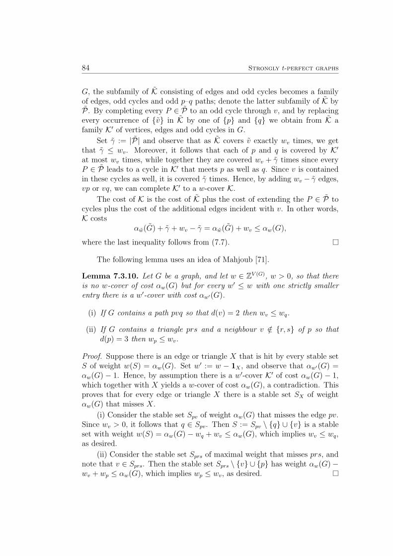
84 Strongly t-perfect graphs
G, the subfamily of K consisting of edges and odd cycles becomes a familyof edges, odd cycles and odd p–q paths; denote the latter subfamily of K byP . By completing every P ∈ P to an odd cycle through v, and by replacingevery occurrence of v in K by one of p and q we obtain from K afamily K′ of vertices, edges and odd cycles in G.
Set γ := |P| and observe that as K covers v exactly wv times, we getthat γ ≤ wv. Moreover, it follows that each of p and q is covered by K′at most wv times, while together they are covered wv + γ times since everyP ∈ P leads to a cycle in K′ that meets p as well as q. Since v is containedin these cycles as well, it is covered γ times. Hence, by adding wv − γ edges,vp or vq, we can complete K′ to a w-cover K.
The cost of K is the cost of K plus the cost of extending the P ∈ P tocycles plus the cost of the additional edges incident with v. In other words,K costs
αw(G) + γ + wv − γ = αw(G) + wv ≤ αw(G),
where the last inequality follows from (7.7).
The following lemma uses an idea of Mahjoub [71].
Lemma 7.3.10. Let G be a graph, and let w ∈ ZV (G), w > 0, so that thereis no w-cover of cost αw(G) but for every w′ ≤ w with one strictly smallerentry there is a w′-cover with cost αw′(G).
(i) If G contains a path pvq so that d(v) = 2 then wv ≤ wq.
(ii) If G contains a triangle prs and a neighbour v /∈ r, s of p so thatd(p) = 3 then wp ≤ wv.
Proof. Suppose there is an edge or triangle X that is hit by every stable setS of weight w(S) = αw(G). Set w′ := w − 1X , and observe that αw′(G) =αw(G) − 1. Hence, by assumption there is a w′-cover K′ of cost αw(G) − 1,which together with X yields a w-cover of cost αw(G), a contradiction. Thisproves that for every edge or triangle X there is a stable set SX of weightαw(G) that misses X.
(i) Consider the stable set Spv of weight αw(G) that misses the edge pv.Since wv > 0, it follows that q ∈ Spv. Then S := Spv \ q ∪ v is a stableset with weight w(S) = αw(G)− wq + wv ≤ αw(G), which implies wv ≤ wq,as desired.
(ii) Consider the stable set Sprs of maximal weight that misses prs, andnote that v ∈ Sprs. Then the stable set Sprs \ v ∪ p has weight αw(G)−wv + wp ≤ αw(G), which implies wp ≤ wv, as desired.
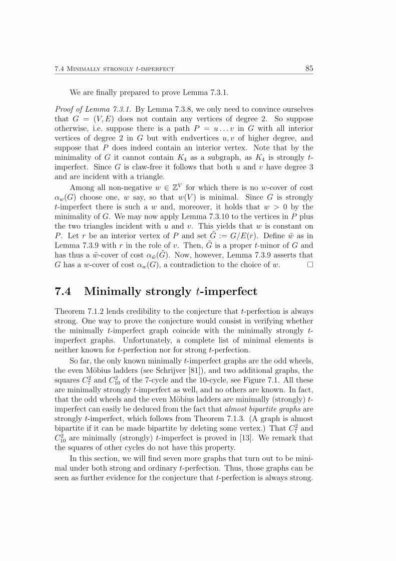
7.4 Minimally strongly t-imperfect 85
We are finally prepared to prove Lemma 7.3.1.
Proof of Lemma 7.3.1. By Lemma 7.3.8, we only need to convince ourselvesthat G = (V,E) does not contain any vertices of degree 2. So supposeotherwise, i.e. suppose there is a path P = u . . . v in G with all interiorvertices of degree 2 in G but with endvertices u, v of higher degree, andsuppose that P does indeed contain an interior vertex. Note that by theminimality of G it cannot contain K4 as a subgraph, as K4 is strongly t-imperfect. Since G is claw-free it follows that both u and v have degree 3and are incident with a triangle.
Among all non-negative w ∈ ZV for which there is no w-cover of costαw(G) choose one, w say, so that w(V ) is minimal. Since G is stronglyt-imperfect there is such a w and, moreover, it holds that w > 0 by theminimality of G. We may now apply Lemma 7.3.10 to the vertices in P plusthe two triangles incident with u and v. This yields that w is constant onP . Let r be an interior vertex of P and set G := G/E(r). Define w as inLemma 7.3.9 with r in the role of v. Then, G is a proper t-minor of G andhas thus a w-cover of cost αw(G). Now, however, Lemma 7.3.9 asserts thatG has a w-cover of cost αw(G), a contradiction to the choice of w.
7.4 Minimally strongly t-imperfect
Theorem 7.1.2 lends credibility to the conjecture that t-perfection is alwaysstrong. One way to prove the conjecture would consist in verifying whetherthe minimally t-imperfect graph coincide with the minimally strongly t-imperfect graphs. Unfortunately, a complete list of minimal elements isneither known for t-perfection nor for strong t-perfection.
So far, the only known minimally t-imperfect graphs are the odd wheels,the even Mobius ladders (see Schrijver [81]), and two additional graphs, thesquares C2
7 and C210 of the 7-cycle and the 10-cycle, see Figure 7.1. All these
are minimally strongly t-imperfect as well, and no others are known. In fact,that the odd wheels and the even Mobius ladders are minimally (strongly) t-imperfect can easily be deduced from the fact that almost bipartite graphs arestrongly t-imperfect, which follows from Theorem 7.1.3. (A graph is almostbipartite if it can be made bipartite by deleting some vertex.) That C2
7 andC2
10 are minimally (strongly) t-imperfect is proved in [13]. We remark thatthe squares of other cycles do not have this property.
In this section, we will find seven more graphs that turn out to be mini-mal under both strong and ordinary t-perfection. Thus, those graphs can beseen as further evidence for the conjecture that t-perfection is always strong.
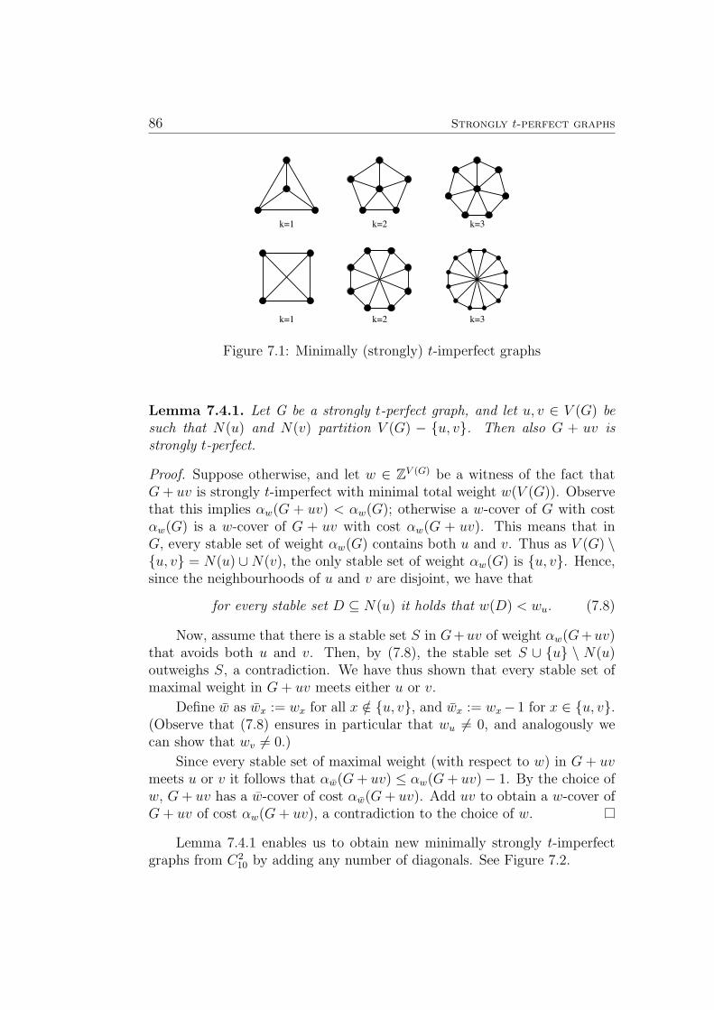
86 Strongly t-perfect graphs
k=3
k=3
k=2k=1
k=2k=1
Figure 7.1: Minimally (strongly) t-imperfect graphs
Lemma 7.4.1. Let G be a strongly t-perfect graph, and let u, v ∈ V (G) besuch that N(u) and N(v) partition V (G) − u, v. Then also G + uv isstrongly t-perfect.
Proof. Suppose otherwise, and let w ∈ ZV (G) be a witness of the fact thatG+ uv is strongly t-imperfect with minimal total weight w(V (G)). Observethat this implies αw(G + uv) < αw(G); otherwise a w-cover of G with costαw(G) is a w-cover of G + uv with cost αw(G + uv). This means that inG, every stable set of weight αw(G) contains both u and v. Thus as V (G) \u, v = N(u) ∪N(v), the only stable set of weight αw(G) is u, v. Hence,since the neighbourhoods of u and v are disjoint, we have that
for every stable set D ⊆ N(u) it holds that w(D) < wu. (7.8)
Now, assume that there is a stable set S in G+uv of weight αw(G+uv)that avoids both u and v. Then, by (7.8), the stable set S ∪ u \ N(u)outweighs S, a contradiction. We have thus shown that every stable set ofmaximal weight in G+ uv meets either u or v.
Define w as wx := wx for all x /∈ u, v, and wx := wx− 1 for x ∈ u, v.(Observe that (7.8) ensures in particular that wu 6= 0, and analogously wecan show that wv 6= 0.)
Since every stable set of maximal weight (with respect to w) in G + uvmeets u or v it follows that αw(G+ uv) ≤ αw(G+ uv)− 1. By the choice ofw, G+ uv has a w-cover of cost αw(G+ uv). Add uv to obtain a w-cover ofG+ uv of cost αw(G+ uv), a contradiction to the choice of w.
Lemma 7.4.1 enables us to obtain new minimally strongly t-imperfectgraphs from C2
10 by adding any number of diagonals. See Figure 7.2.
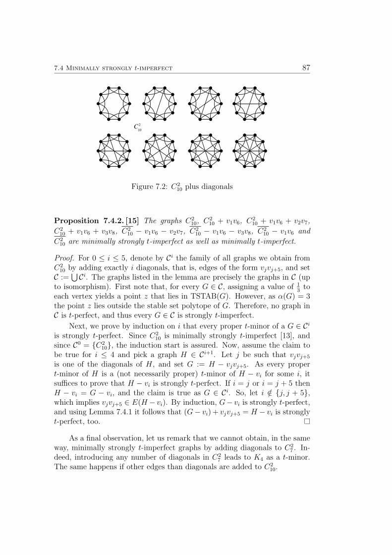
7.4 Minimally strongly t-imperfect 87
10C2
Figure 7.2: C210 plus diagonals
Proposition 7.4.2. [15] The graphs C210, C2
10 + v1v6, C210 + v1v6 + v2v7,
C210 + v1v6 + v3v8, C2
10 − v1v6 − v2v7, C210 − v1v6 − v3v8, C2
10 − v1v6 and
C210 are minimally strongly t-imperfect as well as minimally t-imperfect.
Proof. For 0 ≤ i ≤ 5, denote by Ci the family of all graphs we obtain fromC2
10 by adding exactly i diagonals, that is, edges of the form vjvj+5, and setC :=
⋃ Ci. The graphs listed in the lemma are precisely the graphs in C (upto isomorphism). First note that, for every G ∈ C, assigning a value of 1
3to
each vertex yields a point z that lies in TSTAB(G). However, as α(G) = 3the point z lies outside the stable set polytope of G. Therefore, no graph inC is t-perfect, and thus every G ∈ C is strongly t-imperfect.
Next, we prove by induction on i that every proper t-minor of a G ∈ Ciis strongly t-perfect. Since C2
10 is minimally strongly t-imperfect [13], andsince C0 = C2
10, the induction start is assured. Now, assume the claim tobe true for i ≤ 4 and pick a graph H ∈ Ci+1. Let j be such that vjvj+5
is one of the diagonals of H, and set G := H − vjvj+5. As every propert-minor of H is a (not necessarily proper) t-minor of H − vi for some i, itsuffices to prove that H − vi is strongly t-perfect. If i = j or i = j + 5 thenH − vi = G − vi, and the claim is true as G ∈ Ci. So, let i /∈ j, j + 5,which implies vjvj+5 ∈ E(H − vi). By induction, G− vi is strongly t-perfect,and using Lemma 7.4.1 it follows that (G− vi) + vjvj+5 = H − vi is stronglyt-perfect, too.
As a final observation, let us remark that we cannot obtain, in the sameway, minimally strongly t-imperfect graphs by adding diagonals to C2
7 . In-deed, introducing any number of diagonals in C2
7 leads to K4 as a t-minor.The same happens if other edges than diagonals are added to C2
10.
88 Strongly t-perfect graphs
Chapter 8
Infinite extremal graph theory
8.1 An introduction to infinite extremal graph
theory
From now on, we will shift our focus to infinite graphs. In this chapter,we will take a first approach to infinite extremal graph theory. Necessaryconcepts of infinite graph theory will be introduced along the way.
We will take our first steps in infinite extremal graph theory accompaniedby a well-known result of Kostochka [31], which will serve as an example of thedifficulties one encounters when trying to extend a ‘finite’ result to infinitegraphs. The function f(k) in the theorem is essentially the best possiblebound [89].
Theorem 8.1.1.[Kostochka] There is a constant c so that, for every k ∈ N,if G is a finite graph of average degree at least f(k) := ck
√log k, then G has
a complete minor of order k.
How might this result extend to infinite graphs? First of all we have tonote that it is not clear what the average degree of an infinite graph shouldbe. We shall thus stick to the minimal degree as our ‘density-indicating’parameter. A minor, on the other hand, is defined in same way as for finitegraphs, only that the branch-sets may now be infinite.1
In rayless graphs we will then get a verbatim extension of Theorem 8.1.1(see Chapter 10). In graphs with rays, however, large minimal degree at thevertices is too weak to force any interesting substructure. This is so because
1As long as our minors are locally finite, however (which will always be the case here),it does not make any difference whether we allow infinite branch-sets or not. It is easy tosee that in this case any infinite branch-set may be restricted to a finite one.
90 Infinite extremal graph theory
infinite trees may have arbitrarily large degrees, but they do not even haveany 2-connected subgraphs.
So at first sight, our goal seems unreachable. At second thought, how-ever, the example of the infinite tree just shows that we did not translate theterm ‘large local densities’ in the right way to infinite graphs. Only havingevery finite part of an infinite graph send out a large number of edges willnot produce large overall density, if we do not require something to ‘comeback’ from infinity.
The most natural way to do this is to impose a condition on the endsof the graph. Ends are defined as the equivalence classes of rays (one-wayinfinite paths), under the equivalence relation of not being separable by anyfinite set of vertices. Ends have a long history, see [31, 59].
In [17] and in [86], end degrees were introduced (see also [31, 84]). Infact, two notions have turned out useful (for different purposes): the vertex-degree and the edge-degree of an end ω. The vertex-degree of ω is definedas the maximum cardinality of a set of (vertex)-disjoint rays in ω, and theedge-degree is defined as the maximum cardinality of a set of edge-disjointrays in ω. These maxima exist [49].
Do these notions help to force density in infinite graphs? To some extentthey do: A large minimum degree at the vertices together with a large min-imum vertex-/edge-degree at the ends implies a certain dense substructure,which takes the form of a highly connected or edge-connected subgraph.
More precisely, there is a function fv such that every graph of mini-mum degree resp. vertex-degree fv(k) at the vertices and the ends has ak-connected subgraph, and there is also a function fe such that every graphof minimum degree/edge-degree fe(k) at the vertices and the ends has ak-edge-connected subgraph. While fe is linear, fv is quadratic, and this isalmost best possible. All these results are from [86] and will be presented inChapter 9.
Some related results will already be discussed in Sections 8.3 and 8.4 ofthe present chapter. In Section 8.3 we shall see that independently of thedegrees at the vertices, large vertex-degrees at the ends force an interestingplanar substructure: An end of infinite vertex-degree produces the N × N-grid as a minor [49], and an end of vertex-degree at least 3
2k − 1 forces a
[k] × N-grid-minor. We shall also show that this bound is best possible.In Section 8.4, we shall see that in locally finite vertex-transitive graphs,k-connectivity is implied by much weaker assumptions. In fact, the k-(edge)-connectivity of a locally finite vertex-transitive graph is equivalent to all itsends having vertex-(resp. edge)-degree k.
However, our notion of vertex-/edge-degrees is not strong enough to
8.2 Terminology for infinite graphs 91
make an extension of Theorem 8.1.1 possible. This can be seen by taking theinfinite r-regular tree and inserting the edge set of some spanning subgraphat each level (Example 10.3.1). With a little more effort we can transformour example into one with infinitely many ends of large but finite vertex-/edge-degree (Example 10.3.2).
To overcome this problem, we introduce in Section 10.4 a new end de-gree notion, the relative degree, that makes an extension of Theorem 8.1.1 toinfinite locally finite graphs possible (Theorem 10.4.3). Moreover, every lo-cally finite graph of minimum degree/relative degree k has a finite subgraphof average degree k (Theorem 10.4.2). An application of Theorem 10.4.3 isinvestigated in Section 10.5, where we ask whether as in finite graphs, largegirth can be used to force large complete minors. A partial answer is givenby Proposition 10.5.2.
8.2 Terminology for infinite graphs
All our notation is as in [31], but we take the oppotunity here to remind thereader of the few less standard concepts.
One of the main concepts in infinite graph theory is that of the ends ofa graph G. An end of G is an equivalence class of rays (i.e. one-way infinitepaths) of G, where we say that two rays are equivalent if no finite set ofvertices separates them. We denote the set of ends of a graph G by Ω(G).
The vertex-degree and the edge-degree of an end ω ∈ Ω(G) were intro-duced in [17] resp. in [85]. Sometimes, one refers to both at the same timespeaking informally of the end degree. The vertex-degree dv(ω) of ω is de-fined as the maximum cardinality of a set of (vertex)-disjoint rays in ω, andthe edge-degree de(ω) of ω is defined as the maximum cardinality of a setof edge-disjoint rays in ω. These maxima exist [49], see also [31]. Cleary,the vertex-degree of an end is at most its edge-degree. We shall encounter athird end degree notion in Section 10.4.
For a subgraph H of a graph G, we write ∂vH := N(G − H) for itsvertex-boundary. Similarly, ∂eH := E(H,G−H) is the edge-boundary of H.
An induced connected subgraph H of an infinite graph that has a finitevertex-boundary is called a region. If H contains rays of an end ω, we willsay that H is a region of ω.
For k ∈ N, a separator of a graph of size k will often be called a k-separator, and k-cuts are defined analogously. We say that a separator (orcut) S of a graph G separates some set A ⊆ V (G) from an end ω ∈ Ω(G), ifthe component of G− S that contains rays of ω does not meet A.
92 Infinite extremal graph theory
8.3 Grid minors
From now on, we will deal with graphs that may have rays. We have alreadyseen in the introduction to this chapter that then large degrees at the verticesare not enough to forcesomething as simple as cycles. We shall thus useadditionally the end degrees in order to force interesting substructures ininfinite graphs. In this section, we start modestly by asking for minors thatare planar.
Particularly interesting planar graphs are the grids. The infinite gridZ × Z is the graph on Z2 having all edges of the form (m,n)(m + 1, n) andof the form (m,n)(m,n+ 1), for m,n ∈ Z. The half-grid N×Z, the quarter-grid N× N, and the [k]× N-grid are the induced subgraphs of Z× Z on therespective sets.
A well-known result in infinite graph theory concerns the quarter-grid2,which is a minor of every graph that has an end of infinite vertex-degree (thisis a classical result of Halin [49] who called such ends thick ends).
Theorem 8.3.1 (Halin [49]). Let G be graph which has an end ω of infinitevertex-degree. Then the N× N-grid is a minor of G.
From Halin’s proof it follows that the rays of the subgraph of G thatcan be contracted to N × N belong to ω (see also the proof in Diestel’sbook [31]). On the other hand, it is clear that if a subdivision of the quarter-grid appears as a subgraph of some graph G, the its rays belong to an endof infinite vertex-degree in G.
Thus, it is not surprising that assuming large (but not infinite) degreesand vertex-degrees we cannot force a quarter-grid minor. One example isthe graph G′k from Example 10.3.2, whcih has the additional quality of beingplanar.
However, both graphs contain something quite similar to a quarter-grid:a [k]× N grid, where k depends on the minimum vertex-degree we requiredat the ends. In fact, such a grid always appears in a graph with an end ωof large enough vertex-degree. It will follow from the proof that the rayscorresponding to the rays of the minor, in G belong to ω.
Theorem 8.3.2.[83] Let k ∈ N and let G be graph which has an end ω ofvertex-degree at least 3
2k − 1. Then the [k]× N-grid is a minor of G.
2Observe that when considering minors, it makes no difference whether we work withthe half-grid or the quarter-grid, since, as one easily checks, each of the two is a minor ofthe other.
8.3 Grid minors 93
The bound on the vertex-degree is sharp. This is illustrated by Exam-ple 8.3.3, after the proof of Theorem 8.3.2.
Proof of Theorem 8.3.2. We shall proceed by induction on k. For k = 1 andk = 2, the assertion clearly holds, so assume that k ≥ 3 and that ω is an endof a graph G with dv(ω) ≥ 3
2k − 1.
Choose a set R of dv(ω) disjoint rays from ω. Consider the auxiliarygraph H with V (H) := R where two vertices R and R′ are adjacent ifthere exists an infinite set of disjoint V (R)–V (R′) paths in G which avoidall R′′ ∈ R with R′′ 6= R,R′. Let T be a spanning tree of H. Clearly, if Thappens to be a path, it is easy to construct the desired minor.
So suppose otherwise. Then T has (at least) three leaves R1, R2, R3.Observe that the graph G′ := G− V (
⋃j=1,2,3Rj) has an end ω′ of degree
dv(ω′) = dv(ω)− 3 ≥ 3
2k − 4 =
3
2(k − 2)− 1
whose rays, when viewed in G, belong to ω. Hence, by induction, the [k −2] × N-grid is a minor of G′. In other words, G′ contains a set of raysQ1, Q2, . . . Qk−2 ∈ ω′, and furthermore, each Qi is linked to Qi+1 by infinitelymany disjoint paths, which do not meet any other Qj.
In G, the Qi belong to ω. Thus, since |R| = dv(ω), each Qi meets⋃R
infinitely often. Hence each Qi meets (at least) one of the rays in R, whichwe shall denote by R(Qi), infinitely often.
The tree T from above contains three paths Pi, i = 1, 2, 3, so that Pistarts in V (Ri) and ends in
⋃k−2i=1 V (R(Qi)). Since R1, R2 and R3 are leaves
of T , the Pi can be chosen so that they are disjoint except possibly in theirendvertices. Using the path systems in G represented by the Pi, it is noweasy to see that for each Rj, j = 1, 2, 3, there is a Qij among the Qi such thatthere exist an infinite family of disjoint V (Rj)–V (Qij ) paths which avoid allother Qi′ and Rj′ . Say i1 ≤ i2 ≤ i3.
In order to see that the [k]×N-grid is a minor of G, we shall now definea family of rays Q1, Q2, . . . Qk ∈ ω so that Qi and Qi+1 are connected byinfinitely many disjoint paths which do not meet any other Qi. For i < i1 setQi := Qi, and for i > i3 + 2 set Qi := Qi−2. Set Qi2+1 := R2. For i 6= i2 + 1with i1 < i < i3 + 2, we choose Qi as a suitable ray which alternatively visitsQi−1 and Qi, if i ≤ i2, or Qi−2 and Qi−1, if i > i2 + 1. Finally, Qi1 and Qi3+2
are chosen so that they alternate between R1 and Qi1 , respectively betweenQi3 and R3. Clearly this choice of the rays Qi ensures that, together withsuitable connecting paths, the Qi may be contracted to a [k]× N-grid.
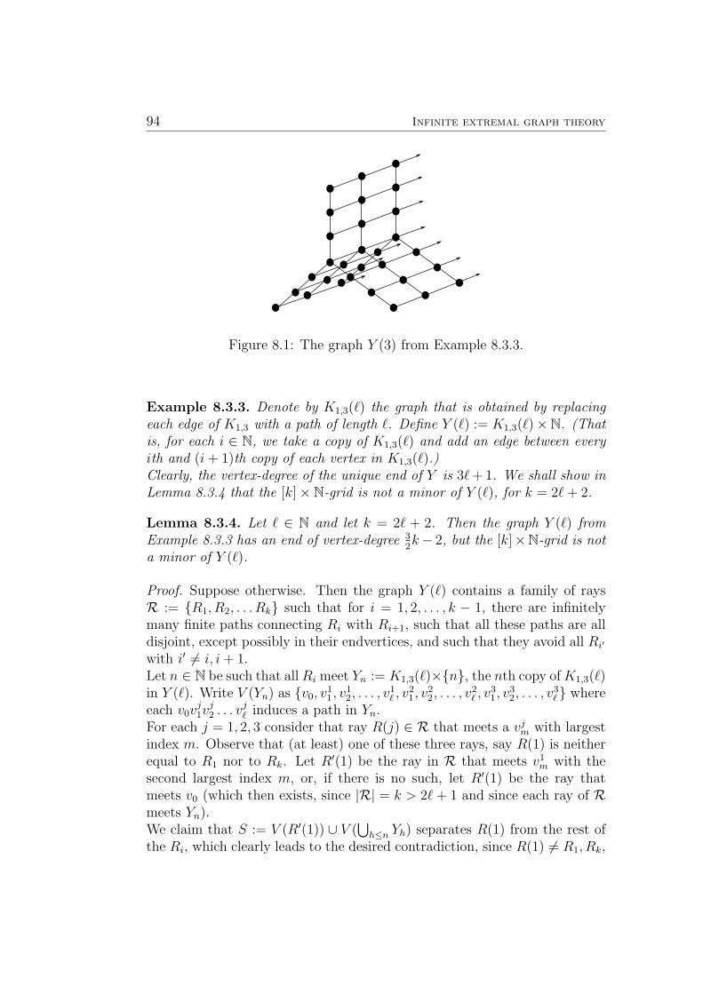
94 Infinite extremal graph theory
Figure 8.1: The graph Y (3) from Example 8.3.3.
Example 8.3.3. Denote by K1,3(`) the graph that is obtained by replacingeach edge of K1,3 with a path of length `. Define Y (`) := K1,3(`)×N. (Thatis, for each i ∈ N, we take a copy of K1,3(`) and add an edge between everyith and (i+ 1)th copy of each vertex in K1,3(`).)Clearly, the vertex-degree of the unique end of Y is 3`+ 1. We shall show inLemma 8.3.4 that the [k]× N-grid is not a minor of Y (`), for k = 2`+ 2.
Lemma 8.3.4. Let ` ∈ N and let k = 2` + 2. Then the graph Y (`) fromExample 8.3.3 has an end of vertex-degree 3
2k− 2, but the [k]×N-grid is not
a minor of Y (`).
Proof. Suppose otherwise. Then the graph Y (`) contains a family of raysR := R1, R2, . . . Rk such that for i = 1, 2, . . . , k − 1, there are infinitelymany finite paths connecting Ri with Ri+1, such that all these paths are alldisjoint, except possibly in their endvertices, and such that they avoid all Ri′
with i′ 6= i, i+ 1.Let n ∈ N be such that allRi meet Yn := K1,3(`)×n, the nth copy ofK1,3(`)in Y (`). Write V (Yn) as v0, v
11, v
12, . . . , v
1` , v
21, v
22, . . . , v
2` , v
31, v
32, . . . , v
3` where
each v0vj1vj2 . . . v
j` induces a path in Yn.
For each j = 1, 2, 3 consider that ray R(j) ∈ R that meets a vjm with largestindex m. Observe that (at least) one of these three rays, say R(1) is neitherequal to R1 nor to Rk. Let R′(1) be the ray in R that meets v1
m with thesecond largest index m, or, if there is no such, let R′(1) be the ray thatmeets v0 (which then exists, since |R| = k > 2`+ 1 and since each ray of Rmeets Yn).We claim that S := V (R′(1)) ∪ V (
⋃h≤n Yh) separates R(1) from the rest of
the Ri, which clearly leads to the desired contradiction, since R(1) 6= R1, Rk,
8.4 Connectivity of vertex-transitive graphs 95
and thus has to be connected to two of the Ri by infinitely many disjointfinite paths that avoid all other Ri. So suppose otherwise, and let P be apath that connects R(1) in Y (`)− S with some Ri∗ ∈ R.By construction of Y (`), this is only possible if R′(1) uses vertices of the typev2m or v3
m. Let n be the smallest index ≥ n such that this occurs, say thenth copy of v2
1 lies on R′(1). Then also the nth copy of v0 lies on R′(1), andfurthermore, all other Ri (with the exception of R(1)) have to pass throughthe nth copies of the vertices v2
2, v23, . . . , v
2` , v
31, v
32, . . . , v
3` . Hence the total
number of rays in R cannot exceed 2`+1, a contradiction, as k = 2`+2.
8.4 Connectivity of vertex-transitive graphs
In the next chapter, we shall se that large degrees at the vertices togetherwith large vertex-/edge-degree at the ends ensure the existence of highlyvertex-/edge-connected subgraphs. In this section, we shall already inves-tigate the same problem for vertex-transitive graphs. As vertex-transitivegraphs are regular, we need no longer use the term ‘mimimum degree’. Thusour question reduces to the following in vertex-transitive graphs: Which de-gree at each vertex do we need in order to ensure that our graph has ak-(edge)-connected subgraph?
It is known that in finite graphs a degree of k is enough, and moreoverthe subgraph will be the graph itself. In fact, every finite vertex-transitivek-regular connected graph is k-edge-connected [64]. It is even k-connected,as long as it does not contain K4 as a subgraph [62].
In infinite graphs, this is no longer true, if we only require degree k atthe vertices, because of the trees. However, if we require a vertex-/edge-degree of at least k at the ends (which is conversely implied by the k-(edge)-connectivity, see below), we can obtain analogous results for infinite locallyfinite graphs. We may even drop the condition on the degrees of the vertices.
Proposition 8.4.1.[83] Let G be an infinite locally finite graph, let k ∈ N.Suppose that G is vertex-transitive and connected.
(a) G is k-connected if and only if all ends of G have vertex-degree at leastk.
(b) G is k-edge-connected if and only if all ends of G have edge-degree atleast k.
In fact, the forward implications in Proposition 8.4.1 are easily impliedby the following result, whose proof is not very difficult and can be foundin [17] for the edge-case (the vertex-case is analogous).
96 Infinite extremal graph theory
Lemma 8.4.2. Let k ∈ N, let G be a locally finite graph, and let ω ∈ Ω(G).Then
(i) dv(ω) = k if and only if k is the smallest integer such that every finiteset S ⊆ V (G) can be separated from ω with a k-separator, and
(ii) de(ω) = k if and only if k is the smallest integer such that every finiteset S ⊆ V (G) can be separated from ω with a k-cut.
Proof of Proposition 8.4.1. Because of Lemma 8.4.2 we only need to provethe backward implications. Let us only prove the implication for (a), for (b)this is analoguous.
Suppose the implication is not true, and let S be an `-separator of G,for some ` < k. Choose a vertex w at distance at least maxdist(u, v) :u, v ∈ S + 1 from all v ∈ S. (Observe that such a vertex w exists, sinceG is infinite, locally finite and connected.) Now, let φ be an automorphismof G that maps some vertex from S to w. Then φ(S) is contained in onecomponent of G− S.
Next, choose an automorphism φ′ that maps φ(w) ‘far away’ from φ(S)to a component of G − φ(S) that does not contain S. Continuing in thismanner, we arrive at a sequence S, φ(S), φ′(φ((S)), φ′′(φ′(φ(S))), . . . of `-separators of G. It is not difficult to construct a ray that meets each of theseseparators and hence defines an end of vertex-degree ` < k. This contradictsour assumption that all ends have vertex-degree at least k.
Chapter 9
Highly connected subgraphs ofinfinite graphs
9.1 The results
In this chapter, which is based on work from [86], we shall state and provethe results on highly connected subgraphs mentioned in the previous chapter.More precisely, we shall prove an infinite analogue of the following well-knowntheorem by Mader.
Theorem 9.1.1 (Mader [66]). Any finite graph G of average degree at least4k has a (k + 1)-connected subgraph.
As we already mentioned earlier, in infinite graphs it does not seem tobe clear what an adequate concept of ‘average degree’ should be, and we willthus restrict ourselves to investigate the consequences of the (in finite graphsstronger) assumption of ‘high minimum degree’.
But as we have seen, simply requiring high degree for the vertices is notenough, as the counterexample of the infinite r-regular tree T r demonstrates.Now, since an infinite tree has rather ‘thin’ ends (which seem to play the roleof the leaves of the infinite tree), this suggests, as conjectured by Diestel [30],that a minimum degree condition has to be imposed also on the ends of thegraph.
In fact, if we require large vertex-degree at the ends, then T r ceases to bea counterexample, as each of its ends has vertex-degree 1. And indeed, withthis further condition on the vertex-degrees of the ends, highly connectedsubgraphs can be forced also in infinite graphs. As our main theorem in thischapter we prove the following infinite analogue:
98 Highly connected subgraphs of infinite graphs
Theorem 9.1.2.[86] Let k ∈ N and let G be a graph such that each vertex hasdegree at least 2k(k+3), and each end has vertex-degree at least 2k(k+1)+1.Then every infinite region of G has a (k + 1)-connected region.
Observe that while in Theorem 9.1.1, the bound on the degrees is linearin k, in Theorem 9.1.2 we require quadratic degree in k. This is in fact nearto best possible:
Theorem 9.1.3.[86] For each k = 5`, where ` ∈ N is even, there exists alocally finite graph whose vertices have degree at least 2` and whose ends havevertex-degree at least ` log `, and which has no (k + 1)-connected subgraph.
In the previous chapter we also defined the edge-degree. It seems thatthe two concepts vertex-degree/edge-degree reflect for ends different aspectsof the degree of a vertex. The vertex-degree of an end is the analogue of thesize of the neighbourhood of a vertex, while the edge-degree corresponds tothe number of incident edges.
This point of view suggests that for forcing highly (vertex-)connectedsubgraphs, high vertex-degree is a more natural requirement than high edge-degree. And in fact, it turns out that high edge-degrees at the ends and highdegrees at the vertices together are not sufficient to force highly connectedsubgraphs, or even highly connected minors, in infinite graphs. In Section 9.4we exhibit for all r ∈ N a locally finite graph of minimum degree and min-imum edge-degree r that has no 4-connected subgraph and no 6-connectedminor.
But, the assumption of high degree and high edge-degree does sufficeto force highly edge-connected subgraphs in arbitrary graphs, with a lowerbound on the (edge)-degrees that is only linear in k:
Theorem 9.1.4.[86] Let k ∈ N and let G be a graph such that each vertexhas degree at least 2k and each end has edge-degree at least 2k. Then G hasa (k + 1)-edge-connected region.
Moreover, highly edge-connected subgraphs can be found in every infi-nite region (Theorem 9.3.2).
In general, it is not possible to force finite highly vertex-/edge-connectedsubgraphs in infinite graphs by assuming high minimum degree and vertex-resp. edge-degree. Neither can one force infinite highly vertex- or edge-connected subgraphs. Counterexamples in this respect are provided in thediscussion after Corollary 9.3.3, near the end of Section 9.3. However, anygraph which obeys the (vertex-/edge)-degree bounds of Theorem 9.1.2 resp.Theorem 9.1.4, has either an infinite (k+1)-vertex-/edge-connected subgraphor infinitely many finite such (see Corollary 9.3.3/Corollary 9.5.2).
9.2 End degrees and more terminology 99
9.2 End degrees and more terminology
The terminology we use is standard, and can be found for example in [31]. A1-way infinite path is called a ray, and the subrays of a ray are its tails. Tworays in a graph G are equivalent if no finite set of vertices separates them;the corresponding equivalence classes of rays are the ends of G. We denotethe set of the ends of G by Ω(G).
Let H be a (possibly empty) subgraph of G, and write H ⊆ G. Theboundary ∂H of H is the set N(G−H) of all neighbours in H of vertices ofG−H. We call H a region (of G) if H is a connected induced subgraph withfinite boundary. Then H ′ ⊆ H is a region of G if and only if it is a region ofH.
Call a region H profound, if V (H) 6= ∂H. For example, all infiniteregions are profound, and a profound region is not empty.
As in finite graphs, we call H k-connected for some k ∈ N, if |H| > k andno set of fewer than k vertices separates H. Similarly, H is k-edge-connectedif |H| > 1 and no set of fewer than k edges separates H. Hence, if H is notk-edge-connected (and non-trivial), then it has a cut of cardinality less thank.
We shall consider two different extensions of the degree notion to ends.The vertex-degree (also known as the multiplicity, or thickness) of an endω ∈ Ω(G) is the maximum cardinality of a set of (vertex)-disjoint rays in ω.The edge-degree of ω (as suggested in [17]) is the maximum cardinality of aset of edge-disjoint rays in ω. It can be shown that these two degree conceptsare well-defined, i.e. the considered maxima do indeed exist.1
9.3 Forcing highly edge-connected subgraphs
The main result of this section (Theorem 9.1.4) is that any graph G of largeenough minimal degree and edge-degree contains a highly edge-connectedsubgraph, which in fact will be a region. We shall then see that such a regionH can be found in any infinite region of G, and that there are either infinitelymany such regions H, or one of infinite order.
Theorem 9.1.4 is best possible in the sense that high edge-degree is not
1Halin [49] proves the existence of an infinite set of disjoint rays if the number ofdisjoint rays in the considered graph is unbounded: with slight modifications, his proofyields the same result for rays of a fixed end. In [17], it is shown that the supremum of thecardinalities of sets of edge-disjoint rays in a given end is attained in locally finite graphs:this proof carries over similarly to arbitrary graphs.
100 Highly connected subgraphs of infinite graphs
sufficient to force highly connected subgraphs, as we shall see in the nextsection.
For the proof, we need the following lemma, which basically assures thatif a graph contains some region with small cut to the outside world, thenthere is either a minimal such, or we have an infinite nested sequence of suchregions so that their cuts are all disjoint.
Lemma 9.3.1. Let D 6= ∅ be a region of a graph G so that |E(D,G−D)| < mand so that |E(D′, G−D′)| ≥ m for every non-empty region D′ ⊆ D−∂D ofG. Then there is an inclusion-minimal region H ⊆ D with |E(H,G−H)| <m and H 6= ∅.Proof. If there is no such H, then we can construct an infinite sequenceof distinct regions D =: D0 ) D1 ) D2 ) . . . such that all cuts Fi :=E(Di, G − Di) have cardinality less than m. Note that any edge that liesin some Fi, but not in Fi+1, lies outside E(Di+1) ∪ Fi+1, and hence will notappear in any Fj with j > i.
By assumption, every region D′ ⊆ D which is not incident with any edgeof F0, sends at least m edges to the outside. Thus, there is an edge e in F0
that appears in all Fi for i ≥ 0. Let E be the set of all edges ej for whichthere exists an index j such that ej ∈ Fi for all i ≥ j. Clearly, e ∈ E, and|E| < m, where the latter follows from the boundedness of the cuts Fi.
Let n be so that E ⊆ Fn. Now, as Dn+1 ( Dn, there is a vertexx ∈ V (Dn−Dn+1). Since Dn is connected, it contains a (finite) path P thatconnects x with y, the endvertex of e in Dn. All Di with i > n contain y,but not x, thus each Fi with i > n must contain one of the edges on P . Thisimplies that there is an edge ej on P which for some j > n lies in all Fi withi ≥ j. Thus, ej ∈ E ⊆ Fn, but Fn ∩ E(P ) = ∅, a contradiction.
We now prove Theorem 9.1.4.
Proof of Theorem 9.1.4. First of all, we shall show that there exists a regionC 6= ∅ such that
(a) |E(C,G− C)| < 2k, and
(b) for every non-empty region C ′ ⊆ C − ∂C we have that|E(C ′, G− C ′)| ≥ 2k.
Indeed, let us construct a sequence C0 ⊇ C1 ⊇ C2 . . . of non-emptyregions such that for i ≥ 0 the following hold
(i) |E(Ci, G− Ci)| < 2k, and
9.3 Forcing highly edge-connected subgraphs 101
(ii) Ci+1 ⊆ Ci − ∂Ci.
Choose C0 as any component of G. Now, if after finitely many, say j,steps of our construction we cannot go on, i.e. find a suitable Cj+1, it isbecause Cj has property (b). Property (a) is then ensured by (i).
So assume that we end up with an infinite sequence C0, C1, C2, . . . ofregions. Observe that, since C0 is a region, ∂Ci 6= ∅ for each i ≥ 1. As eachof the Ci is connected, there is a sequence (Pi)i∈N of ∂Ci–∂Ci+1 paths suchthat for i ≥ 1 the path Pi+1 starts in the last vertex of Pi. By (ii), the pathsPi are non-trivial, and by construction, each Pi meets Pi−1 and Pi+1 only inits first respectively last vertex, and is disjoint from all the other Pj. Hence,their union P :=
⋃∞i=1 Pi is a ray which has a tail in each of the Ci.
Let ω be the end of G that contains P . As, by assumption, ω has edge-degree at least 2k, there is a family R of 2k edge-disjoint ω-rays in G. Foreach ray R ∈ R let nR denote the distance its starting vertex has to ∂C1.Set n := maxnR : R ∈ R+ 2. Then by (ii), all of the 2k disjoint rays in Rstart outside Cn. But each ray in R is equivalent to P , and hence eventuallyenters Cn, contradicting the fact that |E(Cn, G − Cn)| < 2k by (i). Thisproves the existence of a region C 6= ∅ with the properties (a) and (b).
Thus, Lemma 9.3.1 yields an inclusion-minimal non-empty regionH ⊆ Cwith |E(H,G − H)| < 2k. We claim that H is the desired (k + 1)-edge-connected region of G. In fact, otherwise the bound on the degrees of thevertices of G implies that |H| ≥ 2, and so, H has a cut F with |F | ≤ k.We may assume that F is a minimal cut, i.e. splits H into two (non-empty)regions H ′ and H ′′. For one of the two, say H ′, the cut E(H ′, G−H ′) meets
E(H,G−H) in at most |E(H,G−H)|2
< k edges. Hence
|E(H ′, G−H ′)| ≤ |E(H ′, G−H ′) ∩ E(H,G−H)|+ |F | < 2k
and H ′ ( H, contradicting the minimality of H.
Note that our proof yields a (k+1)-edge-connected region in every regionC of G with |E(C,G − C)| < 2k (simply start with C0 := C instead oftaking any component of G). With slightly more effort (and slightly higheredge-degree), one can prove that every infinite region of G contains a (k+1)-edge-connected region:
Theorem 9.3.2. Let k ∈ N, and let G be a graph such that each vertex hasdegree at least 2k, and each end has edge-degree at least 2k + 1. Then everyinfinite region of G contains a (k + 1)-edge-connected region.
102 Highly connected subgraphs of infinite graphs
Proof. Let D be an infinite region of G. If there is a region D′ ⊆ D with|E(D′, G −D′)| ≤ 2k and D 6= ∅, then we proceed as in the proof of Theo-rem 9.1.4 to find an inclusion-minimal non-empty region H with this prop-erty, which then turns out to be the desired (k + 1)-edge-connected region.2
So, we can assume that D contains no non-empty region which sendsless than 2k + 1 edges to the outside. Now, let H ⊆ D be an infinite regionwith |E(H,G−H)| minimal. If we can prove H to be (k+1)-edge-connected,we are done. But otherwise there is a cut F with |F | ≤ k that splits H intotwo regions H ′ and H ′′. At least one of these, say H ′, is infinite. By thechoice of H, the number of edges H ′ sends to the rest of the graph is at least|E(H,G − H)|; hence, E(H ′, G − H ′) contains all but at most |F | edges ofE(H,G−H). Thus,
|E(H ′′, G−H ′′)| = |F ∪ (E(H,G−H)− E(H ′, G−H ′))| ≤ 2k,
contradicting our assumption on D.
Theorem 9.3.2 has two interesting corollaries.
Corollary 9.3.3. Let k ∈ N and let G be a graph in which all vertices havedegree at least 2k, and all ends have edge-degree at least 2k + 1. Then anyinfinite region C of G has either infinitely many disjoint finite (k + 1)-edge-connected regions, or an infinite (k + 1)-edge-connected region.
Proof. Take an inclusion-maximal setD of disjoint finite (k+1)-edge-connectedregions of C (which exists by Zorn’s Lemma), and assume that |D| < ∞.Since any infinite component of C ′ := C −⋃D∈DD ⊆ C is an infinite regionof G, we may use Theorem 9.3.2 to obtain a (k + 1)-edge-connected regionH of C. Then H is infinite by the choice of D.
The two configurations of Corollary 9.3.3 of which one necessarily ap-pears in any given graph of large enough minimal (edge)-degree, need notboth exist, not even in locally finite graphs. Indeed, for given r ∈ N, it is easyto construct an infinite locally finite graph G which has minimum degree andvertex- (and thus edge)- degree r but no infinite 3-edge-connected subgraph.We obtain G from the r × N grid by joining each vertex to r disjoint copiesof Kr+1. Any infinite subgraph of G which is at least 2-edge-connected isalso a subgraph of the r × N grid, and hence is at most 2-edge-connected.
2Observe that, starting with |E(D′, G−D′)| ≤ 2k instead of < 2k, we will have to adjustour inequalities, and the final contradiction is obtained by finding that |E(H ′, G−H ′)| ≤2k.
9.3 Forcing highly edge-connected subgraphs 103
On the other hand, there are also locally finite graphs of high min-imum degree and vertex-degree that have no finite highly edge-connectedsubgraphs. To see this, we reuse an example from the introduction: for givenr ∈ N, add some edges to each level Si of the r-regular tree T r so that in theobtained graph T r each Si induces a path. The only end of T r has infinitevertex- and edge-degree, and the vertices of T r have degree at least r. Now,for every finite subgraph H of T r there is a last level of T r that containsa vertex v of H. Then v has degree at most 3 in H, and hence, H is not4-edge-connected.
Our second corollary of Theorem 9.1.4 describes how the graph G de-composes into subgraphs that either are highly edge-connected or are so thatall their subgraphs send many edges to the outside. For this, we have to pushthe lower bound on the degree of the vertices a little:
Corollary 9.3.4. Let k ∈ N, and let G be a graph whose vertices have degreeat least 4k + 1, and whose ends have edge-degree at least 2k + 1. Then thereis a set D of disjoint (k+1)-edge-connected regions of G such that |E(H,G−H)| ≥ max4k, |H| for each non-empty subgraph H of G−⋃D∈DD.
For the proof, we need the following lemma:
Lemma 9.3.5. Let m ∈ N and let G be a graph such that each of its verticeshas degree at least m. Then every non-empty region H of G with |E(H,G−H)| < m contains at least m+ 1 vertices.
Proof. We may assume that m > 1. Now, we can estimate the number ofedges of H in two ways. On one hand,
‖H‖ ≥ m|H| − |E(H,G−H)|2
>m
2(|H| − 1),
as by assumption, each vertex of H has degree at least m in G. On the otherhand, H cannot have more edges than the complete graph on |H| vertices.
This leaves us with the inequality m2
(|H| − 1) < |H|(|H|−1)2
, implying that|H| > m.
Proof of Corollary 9.3.4. Let D be an inclusion-maximal set D of disjoint(k + 1)-edge-connected regions of G (which again exists by Zorn’s Lemma).
Observe that it suffices to show |E(H,G − H)| ≥ max4k, |H| for in-duced connected non-empty subgraphs H of G−⋃D∈DD, and consider suchan H. If H is infinite, then Theorem 9.3.2 and the (maximal) choice of Dimply that H is not a region of G, i.e. that |E(H,G − H)| is infinite, asdesired.
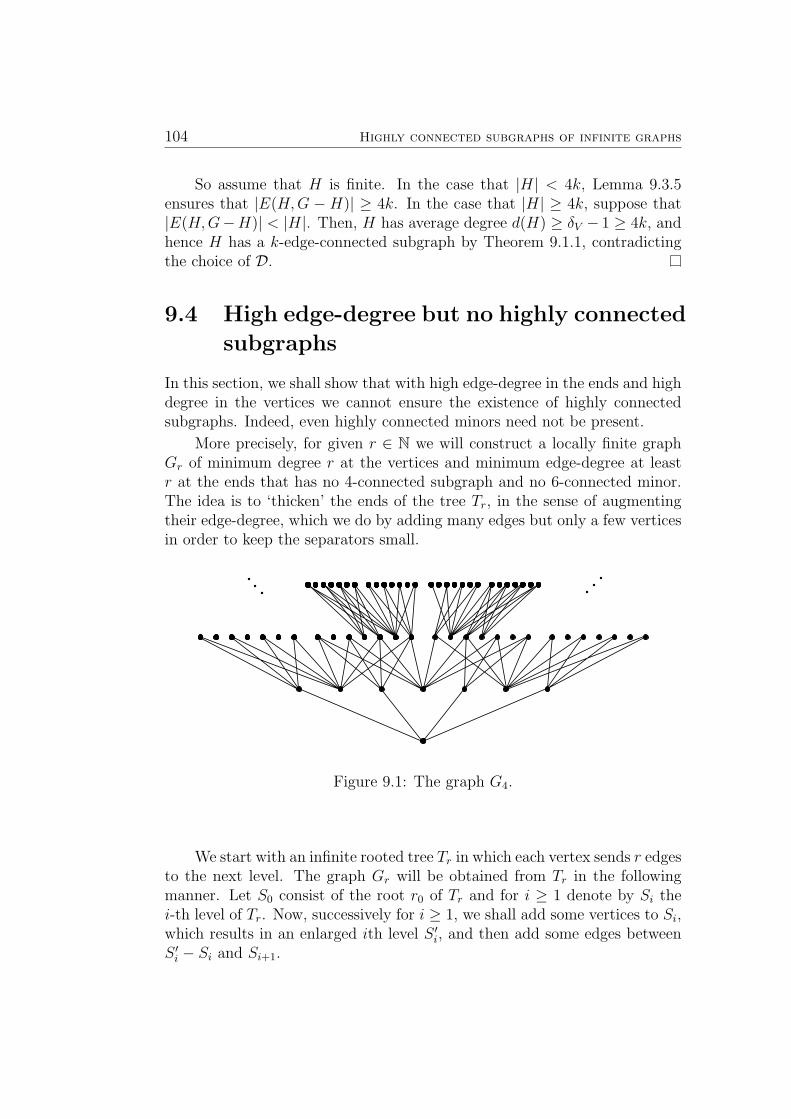
104 Highly connected subgraphs of infinite graphs
So assume that H is finite. In the case that |H| < 4k, Lemma 9.3.5ensures that |E(H,G − H)| ≥ 4k. In the case that |H| ≥ 4k, suppose that|E(H,G−H)| < |H|. Then, H has average degree d(H) ≥ δV − 1 ≥ 4k, andhence H has a k-edge-connected subgraph by Theorem 9.1.1, contradictingthe choice of D.
9.4 High edge-degree but no highly connected
subgraphs
In this section, we shall show that with high edge-degree in the ends and highdegree in the vertices we cannot ensure the existence of highly connectedsubgraphs. Indeed, even highly connected minors need not be present.
More precisely, for given r ∈ N we will construct a locally finite graphGr of minimum degree r at the vertices and minimum edge-degree at leastr at the ends that has no 4-connected subgraph and no 6-connected minor.The idea is to ‘thicken’ the ends of the tree Tr, in the sense of augmentingtheir edge-degree, which we do by adding many edges but only a few verticesin order to keep the separators small.
Figure 9.1: The graph G4.
We start with an infinite rooted tree Tr in which each vertex sends r edgesto the next level. The graph Gr will be obtained from Tr in the followingmanner. Let S0 consist of the root r0 of Tr and for i ≥ 1 denote by Si thei-th level of Tr. Now, successively for i ≥ 1, we shall add some vertices to Si,which results in an enlarged ith level S ′i, and then add some edges betweenS ′i − Si and Si+1.
9.4 High edge-degree but no highly connected subgraphs 105
For each vertex x ∈ Si−1, add r − 1 new vertices vx1 , vx2 , . . . , v
xr−1 to
its neighbourhood Sx = sx1 , sx2 , . . . , sxr in Si. Denote by S ′i the set thusobtained from Si.
Then for each j ≤ r − 1 and each x ∈ Si−1 add all edges between vxjand NSi+1
(sxj , sxj+1). This yields a graph Gr on the disjoint union of setsS ′1, S
′2, . . . as depicted in Figure 9.1 for r = 4.
The ends of Gr correspond to the ends of the underlying tree Tr, i.e. everytwo disjoint rays in Tr belong to different ends of Gr, and each end of Gr
contains a ray from Tr. Indeed, two rays from Tr which in Tr are separatedby⋃ji=0 Si for some j ∈ N, can be separated in Gr by the set
⋃j+1i=0 Si. On
the other hand, every ray R ⊆ Gr has, for any fixed j ∈ N, a tail in exactlyone of the components of G−⋃j
i=0 Si. This tail meets Sxj , for some xj ∈ Sj.Hence R is equivalent to the ray x0x1x2 . . . ⊆ Tr.
Lemma 9.4.1. Gr has minimum degree r at the vertices and minimum edge-degree at least r at the ends.
Proof. The definition of G clearly ensures the desired degree at the vertices.We show that the ends of Gr have edge-degree at least r by constructing aset of r edge-disjoint rays in each. Given an end ω of Gr, there is exactlyone ray R = r0r1r2 . . . ⊆ Tr in it (since the ends of Gr correspond to thoseof Tr, as remarked above).
Now, construct r−1 edge-disjoint ω-rays Ri, where i = 1, . . . , r−1; thesewill also be edge-disjoint from R. Each Ri starts in r0, its second vertex isthe ith neighbour of r0 in S1 which is unused by R. Next, it goes along somepath that switches between S2 and S ′1 until it reaches r2. Note that we canchoose these paths edge-disjoint for different i, for example by letting Ri useonly vertices v ∈ S2 with v = sxi for some x ∈ S1 (or v = r2). Similarly,we continue the Ri going from r2 to the ith unused neighbour in S3, andfrom there along edge-disjoint paths to r4, and so on. Since the Ri agree onr0, r2, r4 . . ., they all belong to ω.
Observe that every finite set A of vertices can be separated from anyend ω by at most three vertices (namely by the neighbours of the uniquecomponent of Gr − S ′i that contains a ray in ω, where j is large enough sothat A ⊆ ⋃j
i=0 S′i). Hence, each end of Gr has vertex-degree at most 3.
In fact, Theorem 9.1.2 ensures that every graph of high minimum degree(at the vertices) has either an end of small vertex-degree or a highly connectedsubgraph. We shall see now that the latter is not the case for Gr.
Lemma 9.4.2. Gr has no 4-connected subgraph.

106 Highly connected subgraphs of infinite graphs
Proof. Suppose otherwise, and let H be a 4-connected subgraph of G. Leti ∈ N so that V (H) ∩ S ′i 6= ∅. Now, if there is a vertex v ∈ V (H)−⋃i+1
j=0 S′i,
then it can be separated in Gr (and thus also in H) from V (H) ∩ S ′i by atmost three vertices, namely by the neighbours of the component of Gr−S ′i+1
that contains v. So, as H is 4-connected, V (H) − ⋃i+1j=0 S
′i must be empty.
Then, there is a maximal j ∈ N such that V (H) ∩ S ′j 6= ∅. But then byconstruction of Gr, any vertex in V (H) ∩ S ′j has degree at most three in H,contradicting the 4-connectedness of H.
It is only slightly more difficult to prove that Gr has no highly connectedminor:
Lemma 9.4.3. Gr has no 6-connected minor.
Proof. Suppose that Gr has a 6-connected minor M . Then there is an n ∈ Nso that each branch-set of M has a vertex in
⋃ni=0 S
′i. Since M is 6-connected,
each separator T ⊆ ⋃ni=0 S
′i ofGr with |T | ≤ 5 leaves a component C ofGr−T
such that V (C) ∪ T meets one and hence every branch-set of M . So as eachS ′i can be separated in Gr from any component of G − S ′i by at most threevertices, there is an i < n such that each branch-set of M meets S ′i ∪ S ′i+1.Moreover, there is a vertex x ∈ Si such that for S := NSi+1
(x) we have thateach branch-set of M has a vertex in S ′ := S ∪ NS′i
(S) ∪ vx1 , vx2 , . . . , vxr−1.Then |S ′ ∩ S ′i| ≤ 3.
Figure 9.2: The graph G′4 for |S ′ ∩ S ′i| = 3.
We claim that M is also a minor of the finite graph G′r (see Figure 9.2)which is obtained from Gr[S
′] by adding an edge between every two verticesthat are neighbours of the same component of Gr − S ′. Indeed, each com-ponent C of Gr − S ′ has at most three neighbours in S ′. Hence, since M is6-connected, C meets only (if at all) those branch-sets of M that also meetNS′(C). It is easy to see that M is still a minor of the graph we obtain fromGr by deleting C and adding all edges between vertices in NS′(C). Arguing
9.5 Forcing highly connected subgraphs 107
analogously for the other components of Gr − S ′, we see that M is also aminor of G′r.
As |S ′ ∩ S ′i| ≤ 3, all but at most 3 branch-sets of M in G′r have alltheir vertices in |S ′ ∩ S ′i+1|. Then these give rise to a 3-connected minor ofG′r−S ′i. But each non-trivial block of G′r−S ′i is a triangle and hence has no3-connected minor, yielding the desired contradiction.
Note that the two latter results are best possible, since Gr has a 3-connected subgraph, the complete graph on 4 vertices, and a 5-connectedminor, the complete graph on 6 vertices.
9.5 Forcing highly connected subgraphs
In this section, we shall prove our main result, Theorem 9.1.2. At first,we shall proceed similarly3 as in the proof of Theorem 9.1.4 (resp. Theo-rem 9.3.2), until we arrive at an infinite region C ′ ⊆ C with the propertythat |∂H| ≥ δΩ holds for all regions H ( C ′. This is achieved in Lemma 9.5.1below.
But then, we see ourselves confronted with new difficulties. The regionC ′ need not be highly connected, or even 2-connected; the reason is that welost control on the degrees of the vertices in C ′. (And the situation onlychanges for the worse if instead of C ′ we consider C ′ − ∂C ′, which needs beneither connected, nor a region.)
Hence, we shall prefer a region H ⊆ C ′ over C ′, if the vertices of ∂Hhave ‘much’ higher degree in H than those of ∂C ′ have in C ′, even if ∂H has‘slightly’ greater cardinality than ∂C ′. This will be formalised below.
Our combination of measurements on the suitability of H, on one hand|∂H|, and on the other, dH(∂H), is responsible for the quadratic lower boundson the degrees which this proof of Theorem 9.1.2 yields. We shall see inSection 9.6 that these bounds are indeed close to best possible.
Lemma 9.5.1. Let G be a graph such that all its ends have vertex-degree atleast δΩ ∈ N. Let C be an infinite region of G. Then there exists a profoundregion C ′ ⊆ C for which one of the following holds:
3The situation here is a little more complicated, because a vertex-version ofLemma 9.3.1, replacing ‘edges’ with ‘vertices’ and ‘cuts’ with ‘separators’, fails, unlesswe make use of the high vertex-degree assumed in Theorem 9.1.2. To see this, take a rayv0v1v2 . . ., to which we add all edges v0vi, and consider the region D which consists of allvi but v1.

108 Highly connected subgraphs of infinite graphs
(a) C ′ is finite and |∂C ′| < δΩ, or
(b) C ′ is infinite and |∂C ′′| ≥ δΩ for every profound region C ′′ ( C ′.
Proof. Suppose otherwise. Then in particular, (b) does not hold for C,i.e. there is a profound region C1 ( C with |∂C1| < δΩ. We shall con-struct a sequence C1 ) C2 ) . . . of profound regions of C so that |∂Cn| < δΩ
for all n ≥ 1.
So assume the region Cn with small boundary has been found. We mayassume Cn to be such that Cn − ∂Cn is connected and also, that N(Cn −∂Cn) = ∂Cn. Indeed, if Cn is not so, we can take any component H ofCn−∂Cn (such a component exists, as Cn is profound) and add N(H) ⊆ ∂Cn.Then H ⊆ Cn is a profound region with the desired small boundary whichwe may use instead of Cn.
As we suppose that (a) does not hold for Cn, we can assume that Cnis infinite. Since Cn is not as required in (b), there is a profound regionCn+1 ( Cn with |∂Cn+1| < δΩ. In this manner, we obtain an infinite sequence(Cn)n∈N.
Denote by V the (possibly empty) set of those vertices v that from somej ∈ N on appear in all ∂Cn with n ≥ j. Since all ∂Cn have size at most δΩ,the set V is finite. Furthermore, as Cn+1 ( Cn for every n ≥ 1, and we chosethe Cn so that Cn − ∂Cn is connected, we have that ∂Cn = V for at mostone n ∈ N. Let J be such that V ( ∂Cn for all n ≥ J .
Observe that for each w ∈ ∂CJ−V there is an index j such that w /∈ ∂Cnfor all n ≥ j. Hence, there is an index J ′ so that ∂CJ ∩ ∂CJ ′ = V . SetC ′1 := CJ , and set C ′2 := CJ ′ . Continuing in this manner, we arrive atan infinite subsequence C ′1 ) C ′2 ) . . . of profound regions of C, whoseboundaries pairwisely meet only in V . Let us summarize the propertieswhich the regions C ′n have, for each n ∈ N:
(i) |∂C ′n| < δΩ,
(ii) C ′n − ∂C ′n is connected, and N(C ′n − ∂C ′n) = ∂C ′n,
(iii) V ( ∂C ′n, and
(iv) ∂C ′n+1 ⊆ (C ′n − ∂C ′n) ∪ V .
We claim that there is a ray R that has a tail in each C ′n. Indeed, by(ii) and (iii), there exists for each n ∈ N a (∂C ′n − V )–(∂C ′n+1 − V ) path Pnsuch that each Pn+1 starts in the last vertex of Pn. By (iv), the paths Pi arenon-trivial, hence, their union is the desired ray R. Denote by ω the end ofG that contains R.
9.5 Forcing highly connected subgraphs 109
As, by assumption, ω has vertex-degree at least δΩ, there is a set R of δΩ
disjoint ω-rays in G. The starting vertices of the rays in R either lie outsideC ′1 − ∂C ′1, or have in C ′1 − V a finite distance to ∂C ′1 − V . Hence, by (iv),there is an N ∈ N so that all rays of R start outside C ′N − ∂C ′N . But (beingequivalent to R) each of these disjoint rays eventually enters C ′N − ∂C ′N , andthus meets ∂C ′N , a contradiction because by (i), |∂C ′N | < δΩ. This completesthe proof of Lemma 9.5.1.
We are now ready to prove the main result of this chapter.
Proof of Theorem 9.1.2. Given an infinite region C of G, we shall find a(k + 1)-connected region H ⊆ C. Theorem 9.1.2 obviously holds for k = 1,since the ends of a tree have vertex-degree 1 < δΩ. We can thus assume thatk > 1.
Suppose there exists a profound finite region D ⊆ C with |∂D| < δΩ.Then D − ∂D has minimum degree at least δ(D − ∂D) ≥ δV − δΩ + 1 = 4k.Hence Theorem 9.1.1 yields a finite (k + 1)-connected subgraph of D ⊆ C,and we are done. Let us therefore assume that there is no such region D.
We may thus apply Lemma 9.5.1 to obtain an infinite region C ′ ⊆ Cwith the property that
|∂C ′′| ≥ δΩ for every profound region C ′′ ( C ′. (9.1)
For a region H ⊆ C ′ write
ΣH :=∑
v∈V (H)
max0, δV − dH(v).
Observe that this sum is finite, since all vertices of H but the finitely manyin ∂H have degree at least δV in H. Now, choose an infinite region H ⊆ C ′
such that (k + 3)|∂H|+ ΣH is minimal.
Assume that there is a vertex v ∈ V (H) that has degree at most 2k − 3in H. Then clearly, v ∈ ∂H. Observe that dH−v(w) = dH(w)− 1 for each ofthe at most 2k − 3 neighbours w of v in H, and dH−v(w
′) = dH(w′) for allother vertices w′ in H. Therefore,
(k + 3)|∂(H − v)|+ ΣH−v ≤ (k + 3)|∂H|+ (k + 3)(2k − 4)
+ ΣH + (2k − 3)− (δV − dH(v))
< (k + 3)|∂H|+ ΣH + 2k(k + 3)− δV= (k + 3)|∂H|+ ΣH .
110 Highly connected subgraphs of infinite graphs
So any infinite component of H−v is a better choice than H, a contradiction.We thus have shown that
dH(v) ≥ 2(k − 1) for each vertex v ∈ V (H). (9.2)
Let us prove now that H is the desired (k + 1)-connected region of C.Indeed, suppose otherwise. Then H has a separator T of cardinality at mostk, which we may assume to be a minimal separator. Note that each suchseparator leaves a component D of H − T such that H ′ := H − D is aninfinite region of C.
Suppose that |V (D) ∩ ∂H| ≥ δΩ − |T |. Then we obtain for the infiniteregion H ′ ⊆ C ′ that
|∂H ′| = |(∂H − V (D)) ∪ T |≤ |∂H| − |V (D) ∩ ∂H|+ |T |≤ |∂H| − δΩ + 2k.
Furthermore,
ΣH′ ≤ ΣH +∑v∈T
max0, δV − dH′(v)
≤ ΣH + kδV ,
and so
(k + 3)|∂H ′|+ ΣH′ ≤ (k + 3)|∂H| − (k + 3)(δΩ − 2k) + ΣH + kδV
< (k + 3)|∂H| − 2k2(k + 3) + ΣH + 2k2(k + 3)
= (k + 3)|∂H|+ ΣH ,
contradicting the choice of H.
Hence,|V (D) ∩ ∂H| < δΩ − |T |.
Thus for the region D := G[V (D) ∪ T ] ⊆ C ′, we have
|∂D| = |(V (D) ∩ ∂H) ∪ T | ≤ |V (D) ∩ ∂H|+ |T | < δΩ.
Observe that D 6= H. So, by (9.1), the region D is not profound, i.e. V (D) =∂D, implying that V (D) ⊆ ∂H. In particular, |D| < δΩ − |T |. Now, for anyvertex v ∈ V (D), we can estimate its degree in H as follows.
dH(v) ≤ |(D ∪ T )− v| < δΩ − 1 = δV − 4k.
9.5 Forcing highly connected subgraphs 111
Then δV − dH(v) > 4k, implying that
ΣH′ ≤ ΣH −∑
v∈V (D)
max0, δV − dH(v)+∑v∈T
(dH(v)− dH′(v))
< ΣH − 4k|D|+ |T ||D|≤ ΣH − 3k.
On the other hand, (9.2) ensures that |D| ≥ 1 + 2(k − 1)− |T | ≥ k − 1.So
|∂H ′| ≤ |∂H| − |D|+ |T | ≤ |∂H|+ 1,
and thus (as k > 1 by assumption)
(k + 3)|∂H ′|+ ΣH′ < (k + 3)|∂H|+ (k + 3) + ΣH − 3k
≤ (k + 3)|∂H|+ ΣH ,
again contradicting the choice of H.
We finish this section with two corollaries of Theorem 9.1.2. The proofof the first is analogous to that of Corollary 9.3.3.
Corollary 9.5.2. Let k ∈ N and let C be an infinite region of a graph G ofminimum degree at least 2k(k+3) at the vertices and minimum vertex-degreeat least 2k(k+ 1) + 1 at the ends. Then C has either infinitely many disjointfinite (k + 1)-connected regions or an infinite (k + 1)-connected region.
Again, these two configurations need not both exist, as the examplesfollowing Corollary 9.3.3 illustrate. (Observe that if a graph has no k-edge-connected subgraph then it clearly has no k-connected subgraph.)
The second corollary of Theorem 9.1.2 is an analogue of Corollary 9.3.4.
Corollary 9.5.3. Let k ∈ N, and let G be a graph whose vertices havedegree at least δV = 2k(k + 3) and whose ends have vertex-degree at leastδΩ = 2k(k+1)+1. Then there is a set D of disjoint (k+1)-connected regionsof G such that |∂H| ≥ maxδΩ,
k−2k|H|+ 1 for each profound subgraph H of
G−⋃D∈DD.
Proof. Similarly as in the proof of Corollary 9.3.4, take an inclusion-maximalset D of disjoint (k + 1)-connected regions of G, and observe that we onlyneed to consider induced connected profound subgraphs H of G−⋃D∈DD.So let H be a such. If H is infinite, then Theorem 9.1.2 and the choice of Dimply that H is not a region, i.e. that |∂H| is infinite, as desired.
112 Highly connected subgraphs of infinite graphs
So assume that H is finite. Then |∂H| ≥ δΩ, as otherwise H − ∂Hhas minimum degree δ(H − ∂H) ≥ δV − δΩ + 1 ≥ 4k, and hence H has a(k+ 1)-connected subgraph by Theorem 9.1.1, contradicting the choice of D.
Also, |∂H| > k−2k|H|. Indeed, suppose otherwise. Then H has average
degree
d(H) ≥ δV |H − ∂H|+ |∂H||H|
≥ δV − (δV − 1)|∂H||H|
≥ 2δV + k − 2
k≥ 4k.
Thus again, Theorem 9.1.1 yields a (k + 1)-connected subgraph of H, acontradiction to the choice of D.
9.6 Linear degree bounds are not enough
Unlike in Mader’s original theorem, and in Theorem 9.1.4, the bounds onthe degrees and vertex-degrees we require in Theorem 9.1.2 are quadratic ink. It seems that our method of proof cannot yield better bounds, becausethe region H we find has to be best possible in two ways: small boundaryon one hand, high in-degree of its vertices on the other. But the quadraticbounds we give are in fact not far from best possible: a minimum degreeand vertex-degree only linear in k is insufficient to ensure (k + 1)-connectedsubgraphs.
Proof of Theorem 9.1.3. Set m := dlog `e. The vertex set of our graph Gwill be that of a tree T , which is rooted in v0. The root has 2` neighbours inthe first level S1 of T , and for i ≥ 1 each vertex in the ith level Si sends twoedges to the next level Si+1. Set S0 := v0. Let ≤ be the order induced bythe tree T on the vertex set V (G) = V (T ), that is, x ≤ y for x, y ∈ V (G) ifand only if x lies on the unique v0–y path in T .
Now, for each i ≥ 0 and each x ∈ Si, add to T all edges xy, wherey ∈ Si+` and y ≥ x. Note that each x 6= v0 has exactly 2` such ‘newneighbours’ y (while v0 has at least that many). Hence, in the thus obtainedgraph G′, each vertex v has degree dG′(v) ≥ 2`.
In order to achieve a high vertex-degree in the ends of the graph, weshall add a few more edges to G′. For this, let us have a closer look at
9.6 Linear degree bounds are not enough 113
T . For j ∈ N, we inductively define sets S(s) ⊆ Sj for each 01-string s oflength j ≥ 1. Divide S1 arbitrarily into two sets S(0), S(1) of equal size (= `).Then for each j ≥ 2, and for each 01-string s of length j − 1, partition theneighbourhood of S(s) in Sj into two sets S(s0), S(s1) of equal size (= `), in away that the neighbourhoods of S(s0) and S(s1) in Sj−1 are disjoint. Then Sjis the disjoint union of all S(s), where s varies over all 01-strings of length j.Now, for each 01-string s of any length, and for each 01-string t of length mmatch S(s0) with S(s1t), and match S(s1) with S(s0t).
This yields a graph G, which we claim to have the desired properties.Indeed, we have seen that already in G′ the vertices have the required degree.Let us now investigate the end structure of G.
We claim that G does not have ‘more’ ends than T , i.e. every end ofG contains a ray from T . Indeed, consider a ray R of G: we shall showthat there is a ray in T which is equivalent to R. Let C0 be the (unique)component of G −⋃m+1
i=1 Si that contains a tail of R. There is a path P0 inT that connects this tail with the unique vertex x0 ∈ S1 for which x0 ≤ c forall c ∈ C0. Now, choose j large enough so that V (P0) ⊆ ⋃j−1
i=0 Si, and let C1
be the component of G−⋃j+mi=1 Si that contains a tail of R. Again, there is
a path P1 in T that connects this tail with the unique vertex x1 ∈ Sj whichsatisfies x1 ≤ c for all c ∈ C1.
Continuing in this manner, we obtain an infinite set of disjoint paths Pi,where each Pi connects xi with V (R). Clearly, since x0 ≤ x1 ≤ x2 ≤ . . .,there is a ray R′ in T that contains all vertices xi. The ray R′ cannot befinitely separated from R, and thus is equivalent to R. Hence, every end ofG contains a ray of T , as desired.4
Next, let us show that the ends of G have vertex-degree at least `m.Given an end ω ∈ Ω(G), and a ray R = v0v1v2 . . . ∈ ω, with R ⊆ T and vi ∈Si for all i, we shall find a set of disjoint rays Ri
j ∈ ω, where i = 1, 2, . . . ,m;and j = 1, 2, . . . , `. These rays will exclusively use edges from E(G)−E(G′).Let s = s1s2s3 . . . be a 01-string of infinite length so that vn ∈ S(s1s2...sn)
for each n ≥ 1. Denote by S(n) the set S(s1s2...sn−1(1−sj)). Now, for fixedi ∈ 1, . . . ,m, the ` disjoint rays Ri
j will pass through all sets S(n), wheren = i, i+m, i+2m, i+3m, . . ., using the S(n)–S(n+m) edges of the matchingfrom the definition of G. This is illustrated in Figure 9.3.
We thus obtain the desired rays Rij for i = 1, 2, . . . ,m and j = 1, 2, . . . , `.
Observe that for each i, j, there are infinitely many disjoint V (R)–V (Rij)
paths in T , namely those that connect vn with the vertex of Rij in S(n+m).
4Moreover, as any two distinct rays of T that start in v0 can be finitely separated inG, we have that the ends of G correspond to the ends of the tree T .
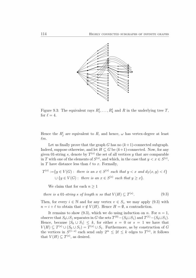
114 Highly connected subgraphs of infinite graphs
Figure 9.3: The equivalent rays R11, . . . , R
14 and R in the underlying tree T ,
for ` = 4.
Hence the Rij are equivalent to R, and hence, ω has vertex-degree at least
`m.
Let us finally prove that the graph G has no (k+1)-connected subgraph.Indeed, suppose otherwise, and let H ⊆ G be (k+1)-connected. Now, for anygiven 01-string s, denote by T (s) the set of all vertices y that are comparablein T with one of the elements of S(s), and which, in the case that y < x ∈ S(s),in T have distance less than ` to x. Formally,
T (s) :=y ∈ V (G) : there is an x ∈ S(s) such that y < x and dT (x, y) < `∪ y ∈ V (G) : there is an x ∈ S(s) such that y ≥ x.
We claim that for each n ≥ 1
there is a 01-string s of length n so that V (H) ⊆ T (s). (9.3)
Then, for every i ∈ N and for any vertex v ∈ Si, we may apply (9.3) withn = i+ ` to obtain that v /∈ V (H). Hence H = ∅, a contradiction.
It remains to show (9.3), which we do using induction on n. For n = 1,observe that S0∪S1 separates in G the sets T (0)−(S0∪S1) and T (1)−(S0∪S1).Hence, because |S0 ∪ S1| ≤ k, for either s = 0 or s = 1 we have thatV (H) ⊆ T (s) ∪ (S0 ∪ S1) = T (s) ∪ S1. Furthermore, as by construction of Gthe vertices in S(1−s) each send only 2m ≤ 2` ≤ k edges to T (s), it followsthat V (H) ⊆ T (s), as desired.
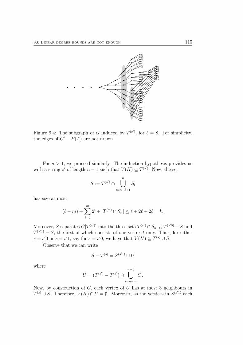
9.6 Linear degree bounds are not enough 115
Figure 9.4: The subgraph of G induced by T (s′), for ` = 8. For simplicity,the edges of G′ − E(T ) are not drawn.
For n > 1, we proceed similarly. The induction hypothesis provides uswith a string s′ of length n− 1 such that V (H) ⊆ T (s′). Now, the set
S := T (s′) ∩n⋃
i=n−`+1
Si
has size at most
(`−m) +m∑i=0
2i + |T (s′) ∩ Sn| ≤ `+ 2`+ 2` = k.
Moreover, S separates G[T (s′)] into the three sets T (s′) ∩Sn−`, T (s′0)−S andT (s′1) − S, the first of which consists of one vertex t only. Thus, for eithers = s′0 or s = s′1, say for s = s′0, we have that V (H) ⊆ T (s) ∪ S.
Observe that we can write
S − T (s) = S(s′1) ∪ Uwhere
U = (T (s′) − T (s)) ∩n−1⋃
i=n−m
Si.
Now, by construction of G, each vertex of U has at most 3 neighbours inT (s) ∪ S. Therefore, V (H) ∩ U = ∅. Moreover, as the vertices in S(s′1) each
116 Highly connected subgraphs of infinite graphs
send only 2m ≤ k edges to T (s)∪S(s′1), it follows that V (H)∩S(s′1) = ∅, andhence, V (H) ⊆ T (s), as desired. This completes the proof of (9.3), and thusthe proof of the theorem.
Chapter 10
Large complete minors ininfinite graphs
10.1 An outline of this chapter
In this chapter, which is based on parts of [83], we shall give a satisfactoryextension of Theorem 8.1.1 for two important classes of infinite graphs. Theseclasses are the rayless and the locally finite graphs.
In infinite graphs, forcing large complete minors only with assumptionson the degrees of the vertices of the graph will not work, as has been explainedin Chapter 8. If we additionally make assumptions on the vertex-/edge-degrees of the ends, then we can force highly (edge)-connected subgraphs,this has been discussed in Chapter 9, but not more: countexexamples shallbe given in Section 10.3.
An exception are the rayless graphs. Proposition 10.2.1 is a verbatimextension of Theorem 8.1.1. This proposition will follow from a useful re-duction theorem (Theorem 10.2.2), which states that every rayless graph ofminimum degree k has a finite subgraph of minimum degree k. These resultswill be presented in Section 10.2.
For infinite locally finite graphs we solve our problem in a different way.As the usual vertex-/edge-degrees do not suffice, we suggest a new notionof an end degree, namely the relative degree, which will be introduced inSection 10.4. With large relative degree, we can force large complete minorsin infinite locally finite graphs (Theorem 10.4.3). Moreover, every locallyfinite graph of minimum degree/relative degree k has a finite subgraph ofaverage degree k (Theorem 10.4.2).
An application of Theorem 10.4.3 is investigated in Section 10.5, where
118 Large complete minors in infinite graphs
we ask whether as in finite graphs, large girth can be used to force largecomplete minors. A partial answer is given by Proposition 10.5.2.
10.2 Large complete minors in rayless graphs
In this section on substructures we shall extend Theorem 8.1.1 to infiniterayless graphs:
Proposition 10.2.1.[28] Let G be a rayless graph such that each vertex hasdegree at least f(r). Then Kr is a minor of G.
In fact, Proposition 10.2.1 follows at once from Theorem 8.1.1 togetherwith the following reduction theorem:
Theorem 10.2.2.[28] Let G be a rayless graph of minimum degree m. ThenG has a finite subgraph of minimum degree m.
In order to prove Theorem 10.2.2, we shall need Konig’s infinity lemma:
Lemma 10.2.3. [31] Let G be a graph on the union of disjoint finite non-empty sets Si, i ∈ N, so that each v ∈ Si has a neighbour in Si−1. Then Ghas a ray.
Proof of Theorem 10.2.2. We start with any finite set S0. For i ≥ 1 we shallchoose for each vertex in Si−1 a set of max0,m neighbours in V (G)\⋃j<i Sj.Let Si be the union of all these sets. Observe that if at some point we setSi = ∅, then, as by assumption each vertex has degree at least m in G, wehave found the desired subgraph of G. On the other hand, if we manage todefine Si for all i ∈ N, we may apply Lemma 10.2.3 to find a ray, contradictingthe assumption that G is rayless.
10.3 Two counterexamples
This section is dedicated to two examples which show that large degree andlarge vertex-degree together are not strong enough assumptions to force largecomplete minors. The difference between the two examples is that the latterdoes not have ends of infinite vertex-degree.
Example 10.3.1. For given k, we take the k-regular tree Tk with levelsL0, L1, L2, . . . and insert the edge set of a spanning cycle Ci at each levelLi of Tk. This can be done in a way so that the obtained graph Gk is still

10.3 Two counterexamples 119
planar.Clearly, Gk has one end of infinite vertex- and edge-degree, and further-more, all vertices of Gk have degree at least k. It is easy to see that Gk isk-connected, but being planar, Gk has no complete minor of order greaterthan 4.
By deleting some (carefully chosen) edges from Gk, we obtain a planargraph of high minimal degree and vertex-degree whose (continuum many)ends all have finite vertex-degree:
Example 10.3.2. Let k ∈ N be given, and consider the graph Gk from Ex-ample 10.3.1. Now, for each i ∈ N, delete the edge vw ∈ E(Ci) from E(Gk),if v and w have no common ancestors in the levels Li−k+2, Li−k+3, . . . , Li−1.Denote the obtained graph by G′k.As Gk is planar, also G′k is. Clearly, k ≤ d(v) ≤ k+2 for each v ∈ V (G). Weshow in Lemma 10.3.3 that the ends of G′k have large, but finite vertex-degree.
Figure 10.1: The graph G′k from Example 10.3.2 for k = 4.
Lemma 10.3.3. The ends of the graph G′k from Example 10.3.2 all havevertex-degree between k − 2 and 2k − 3.
Proof. Consider, for each x ∈ V (G′k) the set
Sx := x ∪⋃
i=1,...,k−2
N i(x),
where N i(x) here denotes the ith neighbourhood of x in level Lm+i, supposingthat x lies in the mth level (of Tk).
120 Large complete minors in infinite graphs
Clearly for each x ∈ V (G′k), the set Sx separates G′k. Hence, already ∂vSx,which has order between k − 1 and 2k − 3, separates G′k.Let us use the sets Sx in order to show that the ends of G′k correspond tothe ends of Tk. In fact, all we have to show is that for each ray R ∈ G′k thereis a ray RT in Tk that is equivalent to R in G′k. We can find such a ray RT
by considering for each i large enough the last vertex vi of R in V (Li). Now,vi ∈ Swi
for exactly one wi ∈ V (Li−k+2). By definition of the vi, the wi areadjacent to their successors wi+1 ∈ V (Li−k+3). So, RT := wkwk+1wk+2 . . . isa ray in Tk as desired.
Thus G′k has continuum many ends, all of which have vertex-degree atmost 2k − 3, because of the separators ∂vSx. It remains to show that eachend ω of G′k has vertex-degree at least k − 2.
For this, fix ω ∈ Ω(G) and consider the union Sω of the sets ∂vSwifor
the ray R = w0w1w2w3 . . . of Tk that lies in ω, where we assume that R startsin L0 = w0. By Lemma 11.4.3, in order to see that ω has vertex-degree atleast k − 2 in G[S] (and thus in G) we only have to show that no set of lessthan k − 2 vertices separates L0 from ω in G[S].
So suppose otherwise, and let T be such a separator. Since every vertexof S has at least k−1 neighbours in the next level, we can reach the 2nd, 3rd,. . . k − 2th level from w0 in G[S]−T . By definition of G′k, these levels containspanning cycles, and thus, as |T | > k−2, there is a wi with i ∈ 1, 2, . . . , k−2which can be reached from w0 in G[S]−T . We repeat the argument with wiin the role of w0, observing that in G[S] ∩ (Li+1 ∪ Li+2 ∪ . . . ∪ Li+k−2), eachlevel contains spanning paths, by construction of G′k.
10.4 Large relative degree forces large com-
plete minors
In the previous sections we explored which substructures may or may not beforced in an infinite graph if we assume large (vertex-)degree at both verticesand ends. In particular we saw that Theorem 8.1.1 (with the average degreereplaced by the minimum degree) does not extend to infinite graphs thathave rays.
In the present section we shall overcome this problem. We will see thatwith a different, more appropriate notion of the end degree a satisfactoryextension of Theorem 8.1.1 is possible.
For this let us first take a closer look at the graph G′k from Exam-ple 10.3.2. Why do the large (vertex-)degrees not interfere with the pla-narity? Observe that, for each finite set S ⊆ V (G), the edge-boundary of
10.4 Large relative degree forces large complete minors 121
the subgraph G′k − S has about the same size as its vertex-boundary. Solocally the density is never large enough to force non-planarity. Similar asin the tree Tk, the density that the high degrees should generate gets losttowards infinity.
In order to avoid this behaviour, we have to prohibit regions R of an endω which have the property that |∂eR|/|∂vR| is small, or at least we shouldprohibit sequences of such regions converging to ω. This is not unnatural:applied to vertices this gives the usual degree, as each vertex v is containedin a smallest region, namely R = v, for which |∂eR|/|∂vR| = d(v).
Let us make our idea more precise. Suppose that G is a locally finitegraph. Write (Hi)i∈N → ω if (Hi)i∈N is an infinite sequence of regions of Gsuch that Hi+1 ⊆ Hi − ∂Hi and ω ∈ H i for each i ∈ N. Observe that suchsequences always exist (as G is locally finite). Define the relative degree ofan end as
de/v(ω) := inf(Hi)i∈N→ω
lim inf|∂eHi||∂vHi| .
Note that by Lemma 11.4.3, in locally finite graphs, we can expressour earlier notions, the vertex- and the edge-degree also using convergingsequences of regions:
dv(ω) = inf(Hi)i∈N→ω
lim inf |∂vHi|, and (10.1)
de(ω) = inf(Hi)i∈N→ω
lim inf |∂eHi|. (10.2)
Our three end degree concepts relate as follows:
Lemma 10.4.1. Let G be a locally finite graph, let ω ∈ Ω(G). Then
de/v(ω) ≤ de(ω)
dv(ω)≤ de(ω).
Proof. The second inequality in trivial. For the first one, let S be the setof starting vertices of a set of disjoint rays of ω that has cardinality dv(ω).Then for each region H ⊆ G− S of ω we have that |∂vH| ≥ dv(ω).
Observe that for the determination of de(ω) using (10.2) it suffices toconsider only sequences of regions Hi that lie in G−S. As each such sequence(Hi)i∈N may be used also to determine de/v(ω), and since for each Hi fromsuch a sequence it holds that
|∂eHi||∂vHi| ≤
|∂eHi|dv(ω)
,
the desired inequality follows.

122 Large complete minors in infinite graphs
With the notion of the relative degree, we can prove a very useful reduc-tion theorem:
Theorem 10.4.2.[28] Let G be a locally finite graph such that each vertexhas degree at least k, and for each end ω we have de/v(ω) ≥ k. Then G hasa finite subgraph H of average degree at least k.
Proof. Choose a vertex v ∈ V (G) and set S0 := v. Inductively we shallconstruct a sequence (Si)i∈N of finite vertex sets. In each step i ≥ 0 weconsider the set Ci of all components C of G− Si with
|∂vC||∂eC| < f(r),
and setSi+1 := Si ∪
⋃C∈Ci
∂vC.
Now, there are two possibilities: either from some i0 on all Si are the same,or they all differ. In the first case observe that G[Si0 ∪N(Si0)] is the desiredsubgraph H. In the second case we may apply Konig’s infinity lemma to finda sequence (Ci)i∈N with Ci ∈ Ci and Ci ⊆ Ci−1 − ∂vCi−1 for i ≥ 1.
It is easy to construct a ray R that passes exactly once through each∂vCi, and hence there is an end ω ∈ ⋂i∈NCi. By construction of the Ci, itfollows that de/v(ω) < f(r), a contradiction.
We may now use Theorem 10.4.2 as a black box in order to translateto infinite locally finite graphs any kind of results from finite graph theorythat make assumptions only on the average or minimum degree. For exam-ple, Theorem 10.4.2 together with Theorem 8.1.1 yields at once the desiredextension of Theorem 8.1.1 to locally finite graphs.
Theorem 10.4.3.[28] Let G be a locally finite graph such that each vertexhas degree at least f(r), and for each end ω we have de/v(ω) ≥ f(r). ThenKr is a minor of G.
Let us remark that we may not weaken the assumption of Theorem 10.4.3in the following sense. Denote by d′e/v the the fraction of the edge- and the
vertex-degree, that is, we set d′e/v(ω) := de(ω)/dv(ω). By Lemma 10.4.1, wehave d′e/v ≥ de/v.
Now, there is no function f ′ such that all graphs with d′e/v(ω), d(v) >
f ′(k) for all ends ω and vertices v contain a complete minor of order k. Thiscan be seen by considering the example from Section 9.4 in the previouschapter.
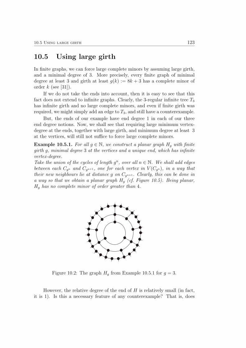
10.5 Using large girth 123
10.5 Using large girth
In finite graphs, we can force large complete minors by assuming large girth,and a minimal degree of 3. More precisely, every finite graph of minimaldegree at least 3 and girth at least g(k) := 8k + 3 has a complete minor oforder k (see [31]).
If we do not take the ends into account, then it is easy to see that thisfact does not extend to infinite graphs. Clearly, the 3-regular infinite tree T3
has infinite girth and no large complete minors, and even if finite girth wasrequired, we might simply add an edge to T3, and still have a counterexample.
But, the ends of our example have end degree 1 in each of our threeend degree notions. Now, we shall see that requiring large minimum vertex-degree at the ends, together with large girth, and minimum degree at least 3at the vertices, will still not suffice to force large complete minors.
Example 10.5.1. For all g ∈ N, we construct a planar graph Hg with finitegirth g, minimal degree 3 at the vertices and a unique end, which has infinitevertex-degree.Take the union of the cycles of length gn, over all n ∈ N. We shall add edgesbetween each Cgn and Cgn+1, one for each vertex in V (Cgn), in a way thattheir new neighbours lie at distance g on Cgn+1. Clearly, this can be done ina way so that we obtain a planar graph Hg (cf. Figure 10.5). Being planar,Hg has no complete minor of order greater than 4.
Figure 10.2: The graph Hg from Example 10.5.1 for g = 3.
However, the relative degree of the end of H is relatively small (in fact,it is 1). Is this a necessary feature of any counterexample? That is, does
124 Large complete minors in infinite graphs
every graph of minimum degree 3 and large girth and without large completeminors have to have an end of small relative degree? At least the relativedegrees cannot be too large:
Proposition 10.5.2.[28] Every locally finite graph G of minimal degree atleast 3 at the vertices, minimal relative degree at least r(k) = ck
√log k at the
ends and girth at least g(k) = 8k + 3 has a complete minor of order k.
Proof. One may employ the same proof as for finite graphs, as given e.g. in [31].The strategy there is to construct first a minor M of G that has large min-imal degree, and then apply Theorem 8.1.1 to M . In an infinite graph, wecan construct the minor M in exactly the same way, and it is not overlydifficult to see that M does not only have large degree at the vertices, butalso has at least the same relative degree at the ends as G. It suffices toapply Theorem 10.4.3 to obtain the desired minor.
How much can this bound be lowered? May we take r(k) to be constant,even r(k) = 3? It would be interesting to find the smallest number r(k) sothat every locally finite graph with d(v) ≥ 3 and de/v(ω) ≥ r(k) for allvertices v and ends ω, and of girth at least g(k) has a complete minor oforder k.

Chapter 11
Minimal k-(edge)-connectivityin infinite graphs
11.1 Four notions of minimality
The minimal degree and bounds on the number of vertices that attain theminimal degree have been much studied for finite graphs that are in certainways minimally k-connected/k-edge-connected. This minimality will havetwo meanings here: minimality upon vertex deletion and upon edge deletion(see below for the precise definition).
In this chapter, which is based on [82], we shall give an overview of theresults known, and show that most carry over to infinite graphs. This ismade possible by considering the (vertex/edge)-degree of the ends as well asthe degree of the vertices.
Four notions will be of interest. For k ∈ N, we shall call a graph Gedge-minimally k-connected, resp. edge-minimally k-edge-connected if G is k-connected resp. k-edge-connected, but G− e is not, for every edge e ∈ E(G).Analogously, call G vertex-minimally k-connected, resp. vertex-minimally k-edge-connected if G is k-connected resp. k-edge-connected, but G− v is not,for every vertex v ∈ V (G).
These four classes of graphs often appear in the literature under thenames of k-minimal/k-edge-minimal/k-critical/k-edge-critical graphs. Over-views of results known for finite graphs and also for digraphs can be foundin [5, 39].
126 Minimal k-(edge)-connectivity in infinite graphs
11.2 The situation in finite graphs
It is known that finite graphs which belong to one of the classes defined abovehave vertices of small degree. In fact, three of the four cases the trivial lowerbound of k on the minimum degree is attained. We summarise the knownresults in the following theorem:
Theorem 11.2.1. Let G be a finite graph, let k ∈ N. Then
(a) (Halin [50]) If G is edge-minimally k-connected, then G has a vertex ofdegree k,
(b) (Lick et al [21], Mader [63]) If G is vertex-minimally k-connected,then G has a vertex of degree 3
2k − 1,
(c) (Lick [60]) If G is edge-minimally k-edge-connected, then G has a vertexof degree k,
(d) (Mader [69]) If G is vertex-minimally k-edge-connected, then G has avertex of degree k.
Note that in Theorem 11.2.1 (b), the bound of 3k/2 − 1 on the degreeis best possible. For even k, this can be seen by replacing each vertex ofC`, a circle of some length ` ≥ 4, with a copy of Kk/2, the complete graphon k/2 vertices, and adding all edges between two copies of Kk/2 when thecorresponding vertices of C` are adjacent. This procedure is sometimes calledthe strong product1 of C` and Kk/2. For odd values of k similar examples canbe constructed, using K(k+1)/2’s instead of Kk/2’s, and in the end deletingtwo vertices which belong to two adjacent copies of K(k+1)/2.
In all four cases of Theorem 1, the minimal degree is attained by morethan one vertex:
Theorem 11.2.2. Let G be a finite graph, let k ∈ N. Then
(a) (Mader [65]) In case (a) of Theorem 11.2.1, G has at least ck|G| verticesof degree k, where ck is a constant depending only on k, unless k = 1, inwhich case G has at least two vertices of degree k,
(b) (Hamidoune [52]) In case (b) of Theorem 11.2.1, if k > 1 then G hasat least two vertices of degree 3
2k − 1,
1The strong product of two graphs H1 and H2 is defined in [55] as the graph on V (H1)×V (H2) which has an edge (u1, u2)(v1, v2) whenever uivi ∈ E(Hi) for i = 1 or i = 2, andat the same time either u3−i = v3−i or u3−iv3−i ∈ E(H3−i).
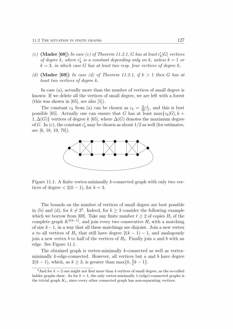
11.2 The situation in finite graphs 127
(c) (Mader [68]) In case (c) of Theorem 11.2.1, G has at least c′k|G| verticesof degree k, where c′k is a constant depending only on k, unless k = 1 ork = 3, in which case G has at least two resp. four vertices of degree k,
(d) (Mader [69]) In case (d) of Theorem 11.2.1, if k > 1 then G has atleast two vertices of degree k.
In case (a), actually more than the number of vertices of small degree isknown: If we delete all the vertices of small degree, we are left with a forest(this was shown in [65], see also [5]).
The constant ck from (a) can be chosen as ck = k−12k−1
, and this is bestpossible [65]. Actually one can ensure that G has at least maxck|G|, k +1,∆(G) vertices of degree k [65], where ∆(G) denotes the maximum degreeofG. In (c), the constant c′k may be chosen as about 1/2 as well (for estimates,see [6, 18, 19, 70]).
Figure 11.1: A finite vertex-minimally k-connected graph with only two ver-tices of degree < 2(k − 1), for k = 3.
The bounds on the number of vertices of small degree are best possiblein (b) and (d), for k 6= 22. Indeed, for k ≥ 3 consider the following examplewhich we borrow from [69]. Take any finite number ` ≥ 2 of copies Hi of thecomplete graph K2(k−1), and join every two consecutive Hi with a matchingof size k−1, in a way that all these matchings are disjoint. Join a new vertexa to all vertices of H1 that still have degree 2(k − 1) − 1, and analogouslyjoin a new vertex b to half of the vertices of H`. Finally join a and b with anedge. See Figure 11.1.
The obtained graph is vertex-minimally k-connected as well as vertex-minimally k-edge-connected. However, all vertices but a and b have degree2(k − 1), which, as k ≥ 3, is greater than maxk, 3
2k − 1.
2And for k = 2 one might not find more than 4 vertices of small degree, as the so-calledladder graphs show. As for k = 1, the only vertex-minimally 1-(edge)-connected graphs isthe trivial graph K1, since every other connected graph has non-separating vertices.
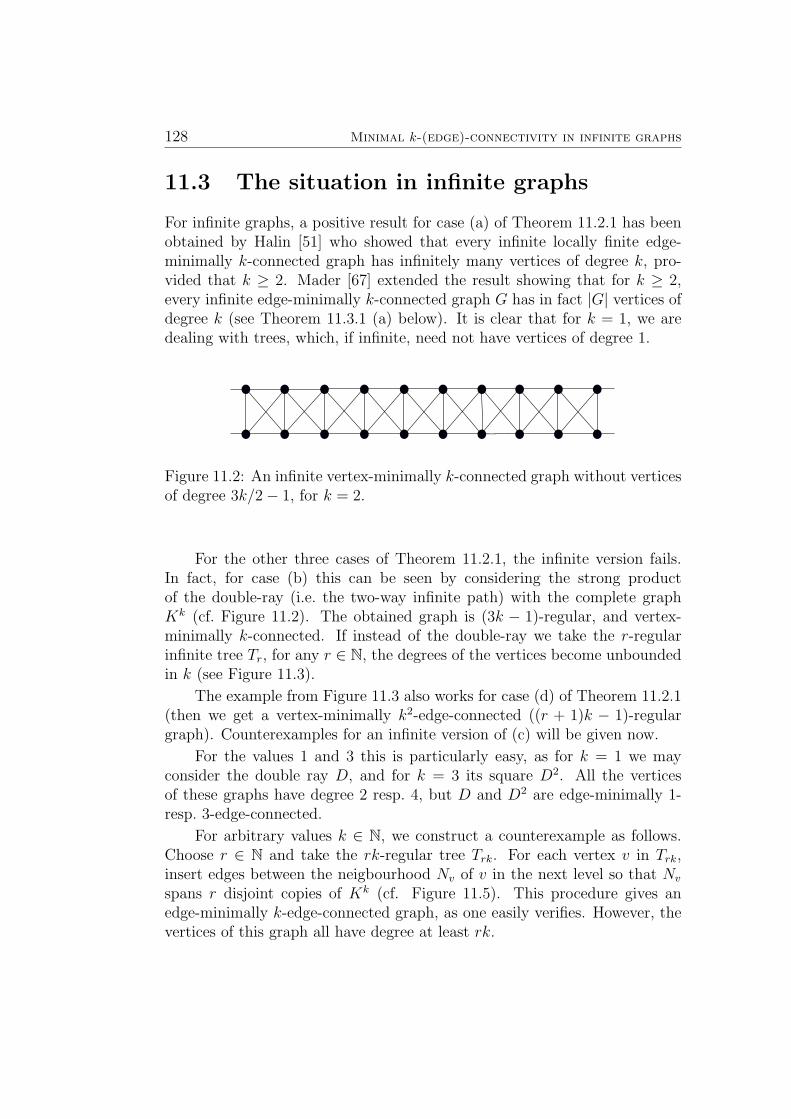
128 Minimal k-(edge)-connectivity in infinite graphs
11.3 The situation in infinite graphs
For infinite graphs, a positive result for case (a) of Theorem 11.2.1 has beenobtained by Halin [51] who showed that every infinite locally finite edge-minimally k-connected graph has infinitely many vertices of degree k, pro-vided that k ≥ 2. Mader [67] extended the result showing that for k ≥ 2,every infinite edge-minimally k-connected graph G has in fact |G| vertices ofdegree k (see Theorem 11.3.1 (a) below). It is clear that for k = 1, we aredealing with trees, which, if infinite, need not have vertices of degree 1.
Figure 11.2: An infinite vertex-minimally k-connected graph without verticesof degree 3k/2− 1, for k = 2.
For the other three cases of Theorem 11.2.1, the infinite version fails.In fact, for case (b) this can be seen by considering the strong productof the double-ray (i.e. the two-way infinite path) with the complete graphKk (cf. Figure 11.2). The obtained graph is (3k − 1)-regular, and vertex-minimally k-connected. If instead of the double-ray we take the r-regularinfinite tree Tr, for any r ∈ N, the degrees of the vertices become unboundedin k (see Figure 11.3).
The example from Figure 11.3 also works for case (d) of Theorem 11.2.1(then we get a vertex-minimally k2-edge-connected ((r + 1)k − 1)-regulargraph). Counterexamples for an infinite version of (c) will be given now.
For the values 1 and 3 this is particularly easy, as for k = 1 we mayconsider the double ray D, and for k = 3 its square D2. All the verticesof these graphs have degree 2 resp. 4, but D and D2 are edge-minimally 1-resp. 3-edge-connected.
For arbitrary values k ∈ N, we construct a counterexample as follows.Choose r ∈ N and take the rk-regular tree Trk. For each vertex v in Trk,insert edges between the neigbourhood Nv of v in the next level so that Nv
spans r disjoint copies of Kk (cf. Figure 11.5). This procedure gives anedge-minimally k-edge-connected graph, as one easily verifies. However, thevertices of this graph all have degree at least rk.
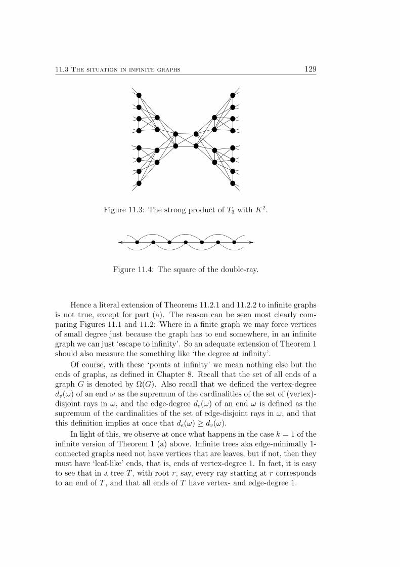
11.3 The situation in infinite graphs 129
Figure 11.3: The strong product of T3 with K2.
Figure 11.4: The square of the double-ray.
Hence a literal extension of Theorems 11.2.1 and 11.2.2 to infinite graphsis not true, except for part (a). The reason can be seen most clearly com-paring Figures 11.1 and 11.2: Where in a finite graph we may force verticesof small degree just because the graph has to end somewhere, in an infinitegraph we can just ‘escape to infinity’. So an adequate extension of Theorem 1should also measure the something like ‘the degree at infinity’.
Of course, with these ‘points at infinity’ we mean nothing else but theends of graphs, as defined in Chapter 8. Recall that the set of all ends of agraph G is denoted by Ω(G). Also recall that we defined the vertex-degreedv(ω) of an end ω as the supremum of the cardinalities of the set of (vertex)-disjoint rays in ω, and the edge-degree de(ω) of an end ω is defined as thesupremum of the cardinalities of the set of edge-disjoint rays in ω, and thatthis definition implies at once that de(ω) ≥ dv(ω).
In light of this, we observe at once what happens in the case k = 1 of theinfinite version of Theorem 1 (a) above. Infinite trees aka edge-minimally 1-connected graphs need not have vertices that are leaves, but if not, then theymust have ‘leaf-like’ ends, that is, ends of vertex-degree 1. In fact, it is easyto see that in a tree T , with root r, say, every ray starting at r correspondsto an end of T , and that all ends of T have vertex- and edge-degree 1.
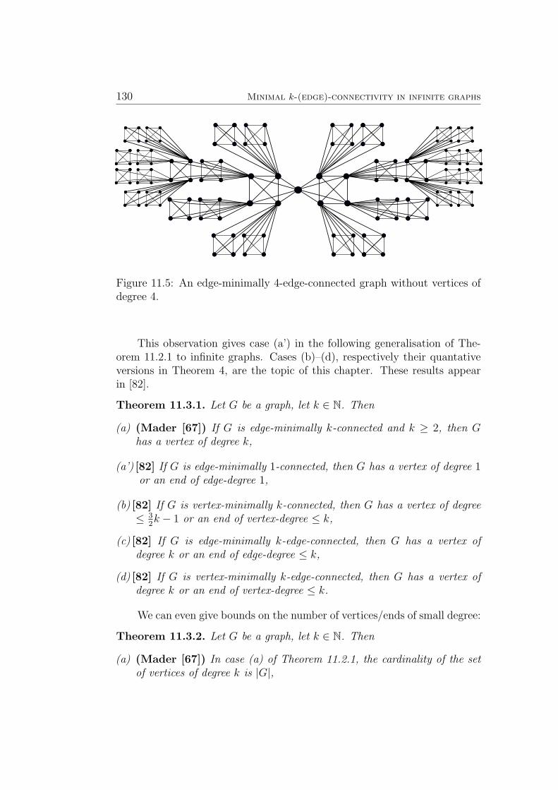
130 Minimal k-(edge)-connectivity in infinite graphs
Figure 11.5: An edge-minimally 4-edge-connected graph without vertices ofdegree 4.
This observation gives case (a’) in the following generalisation of The-orem 11.2.1 to infinite graphs. Cases (b)–(d), respectively their quantativeversions in Theorem 4, are the topic of this chapter. These results appearin [82].
Theorem 11.3.1. Let G be a graph, let k ∈ N. Then
(a) (Mader [67]) If G is edge-minimally k-connected and k ≥ 2, then Ghas a vertex of degree k,
(a’) [82] If G is edge-minimally 1-connected, then G has a vertex of degree 1or an end of edge-degree 1,
(b) [82] If G is vertex-minimally k-connected, then G has a vertex of degree≤ 3
2k − 1 or an end of vertex-degree ≤ k,
(c) [82] If G is edge-minimally k-edge-connected, then G has a vertex ofdegree k or an end of edge-degree ≤ k,
(d) [82] If G is vertex-minimally k-edge-connected, then G has a vertex ofdegree k or an end of vertex-degree ≤ k.
We can even give bounds on the number of vertices/ends of small degree:
Theorem 11.3.2. Let G be a graph, let k ∈ N. Then
(a) (Mader [67]) In case (a) of Theorem 11.2.1, the cardinality of the setof vertices of degree k is |G|,
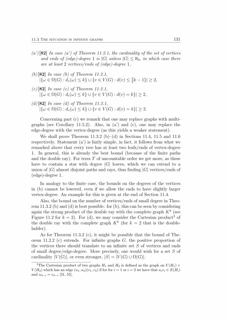
11.3 The situation in infinite graphs 131
(a’) [82] In case (a’) of Theorem 11.2.1, the cardinality of the set of verticesand ends of (edge)-degree 1 is |G| unless |G| ≤ ℵ0, in which case thereare at least 2 vertices/ends of (edge)-degree 1,
(b) [82] In case (b) of Theorem 11.2.1,|ω ∈ Ω(G) : dv(ω) ≤ k ∪ v ∈ V (G) : d(v) ≤ 3
2k − 1| ≥ 2,
(c) [82] In case (c) of Theorem 11.2.1,|ω ∈ Ω(G) : de(ω) ≤ k ∪ v ∈ V (G) : d(v) = k| ≥ 2,
(d) [82] In case (d) of Theorem 11.2.1,|ω ∈ Ω(G) : dv(ω) ≤ k ∪ v ∈ V (G) : d(v) = k| ≥ 2.
Concerning part (c) we remark that one may replace graphs with multi-graphs (see Corollary 11.5.2). Also, in (a’) and (c), one may replace theedge-degree with the vertex-degree (as this yields a weaker statement).
We shall prove Theorem 11.3.2 (b)–(d) in Sections 11.4, 11.5 and 11.6respectively. Statement (a’) is fairly simple, in fact, it follows from what weremarked above that every tree has at least two leafs/ends of vertex-degree1. In general, this is already the best bound (because of the finite pathsand the double ray). For trees T of uncountable order we get more, as thesehave to contain a star with degree |G| leaves, which we can extend to aunion of |G| almost disjoint paths and rays, thus finding |G| vertices/ends of(edge)-degree 1.
In analogy to the finite case, the bounds on the degrees of the verticesin (b) cannot be lowered, even if we allow the ends to have slightly largervertex-degree. An example for this is given at the end of Section 11.4.
Also, the bound on the number of vertices/ends of small degree in Theo-rem 11.3.2 (b) and (d) is best possible: for (b), this can be seen by consideringagain the strong product of the double ray with the complete graph Kk (seeFigure 11.2 for k = 2). For (d), we may consider the Cartesian product3 ofthe double ray with the complete graph Kk (for k = 2 that is the double-ladder).
As for Theorem 11.3.2 (c), it might be possible that the bound of The-orem 11.2.2 (c) extends. For infinite graphs G, the positive proportion ofthe vertices there should translate to an infinite set S of vertices and endsof small degree/edge-degree. More precisely, one would wish for a set S ofcardinality |V (G)|, or even stronger, |S| = |V (G) ∪ Ω(G)|.
3The Cartesian product of two graphs H1 and H2 is defined as the graph on V (H1)×V (H2) which has an edge (u1, u2)(v1, v2) if for for i = 1 or i = 2 we have that uivi ∈ E(Hi)and u3−i = v3−i [31, 55].
132 Minimal k-(edge)-connectivity in infinite graphs
Observe that it is necessary to exclude also in the infinite case the twoexceptional values k = 1 and k = 3, as there are graphs (namely D and D2,see above) with only two vertices/ends of (edge)-degree 1 resp. 3. For othervalues of k, an extension might hold:
Question 11.3.3. Are there k ∈ N for which every infinite edge-minimallyk-edge-connected graph G contains infinitely many vertices or ends of (edge)-degree k? Does G have |V (G)| (or even |V (G)∪Ω(G)|) such vertices or ends?
Another interesting question is which k-(edge)-connected graphs havevertex- or edge-minimally k-(edge)-connected subgraphs. Finite graphs triv-ially do, but for infinite graphs this is not always true. This observationleads to the study of vertex-/edge-minimally k-(edge)-connected (standard)subspaces rather than graphs. For more on this, see [29, 83], the latter ofwhich contains a version of Theorem 3 (a) for standard subspaces.
11.4 Vertex-minimally k-connected graphs
In this section we shall show part (b) of Theorem 11.3.2. For the proof, weneed two lemmas. The first of these lemmas may be extracted from [21] orfrom [67], and at once implies Theorem 11.2.1 (b). For completeness, weshall give a proof.
Lemma 11.4.1. Let k ∈ N, k > 0, let G be a vertex-minimally k-connectedgraph, and let H be a profound finite k-region of G. Then G has a vertex vof degree at most 3
2k − 1.
Moreover, if |G−H| > |H − ∂vH|, then v ∈ V (H).
Proof. Assume that H was chosen inclusion-minimal among all profoundfinite k-regions of G. Set T := ∂vH, set C1 := H − T , and set C2 := G−H.Let x ∈ V (C1), and observe that since G is vertex-minimally k-connected,there is a k-separator T ′ of G with x ∈ T ′. Let D1 be a component of G−T ′,set D2 := G − T ′ − D1, and set T ∗ := T ∩ T ′. Furthermore, for i, j = 1, 2set Aij := Ci ∩ Dj and set T ij := (T ′ ∩ Ci) ∪ (T ∩ Dj) ∪ T ∗. Observe thatN(Aij) ⊆ T ij .
We claim that there are i1, i2, j1, j2 with either (i1, j1) = (i2, 3 − j2) ori1, j1) = (3− i2, j2) such that for (i, j) ∈ (i1, j1), (i2, j2):
|T ij | ≤ k and Aij = ∅. (11.1)
In fact, observe that for j = 1, 2 we have that |T 1j |+|T 2
j | ≤ |T |+|T ′| = 2k.Thus either |T 1
j | ≤ k, which by the minimality of H implies that A1j is empty,
11.4 Vertex-minimally k-connected graphs 133
or |T 2j | < k, which by the k-connectivity of G implies that A2
j is empty. Thisproves (11.1).
We hence know that there is an X ∈ C1, C2, D1, D2 such that V (X) ⊆T∪T ′. Moreover, if X ∈ C1, C2 then |X|∪|T∩D1| ≤ k and |X|∪|T∩D2| ≤k. Since |T | = k, this implies that 2|X| ≤ 2k − |T | = k. In the same waywe get that if X ∈ D1, D2 then 2|X| ≤ 2k − |T ′| = k. Hence, in any casethere is a vertex v ∈ X of degree at most
max|T |+ |X| − 1, |T ′|+ |X| − 1 ≤ k + k/2− 1.
It is easy to see that we may choose v ∈ V (H) unless both |T 11 | and |T 1
2 |are greater than k. But then by (11.1) V (C2) ⊆ T ′, and thus |C2| ≤ k/2 ≤|T ′ ∩ C1| ≤ |C1|, as desired.
We also need Lemma 9.5.1 from Chapter 9. Observe that the outcomeof Lemma 9.5.1 is invariant under modifications of the structure of G − C.Hence we may always assume that dv(ω) ≥ m only for ends ω of G that haverays in C. Let us restate the thus modified lemma:
Lemma 11.4.2. Let G be a graph such that all its ends have vertex-degree atleast m ∈ N. Let C be an infinite region of G. Then there exists a profoundregion C ′ ⊆ C for which one of the following holds:
(a) C ′ is finite and |∂vC ′| < m , or
(b) C ′ is infinite and |∂vC ′′| ≥ m for every profound region C ′′ ( C ′.
We are now ready to prove Theorem 11.3.2 (b).
Proof of Theorem 11.3.2 (b). First of all, we claim that for every infiniteregion H of G it holds that
There is a vertex v ∈ V (H) of degree ≤ 32k − 1 or an end of
vertex-degree ≤ k with rays in H.(11.2)
In order to see (11.2), we assume that there is no end as desired and applyLemma 11.4.2 to H with m := k+ 1. This yields a profound region H ′ ⊆ H.We claim that (a) of Lemma 11.4.2 holds; then we may use Lemma 11.4.1 tofind a vertex w ∈ V (H ′) with d(w) ≤ 3k/2− 1.
So, assume for contradiction that (b) of Lemma 11.4.2 holds. Since G isk-connected there exists a finite family P of finite paths in G such that eachpair of vertices from ∂vH
′ is connected by k otherwise disjoint paths from P .Set
S := ∂vH′ ∪ V (
⋃P),
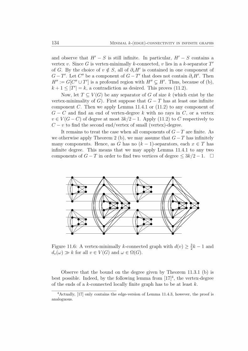
134 Minimal k-(edge)-connectivity in infinite graphs
and observe that H ′ − S is still infinite. In particular, H ′ − S contains avertex v. Since G is vertex-minimally k-connected, v lies in a k-separator T ′
of G. By the choice of v /∈ S, all of ∂vH′ is contained in one component of
G− T ′. Let C ′′ be a component of G− T ′ that does not contain ∂vH′. Then
H ′′ := G[C ′′ ∪ T ′] is a profound region with H ′′ ( H ′. Thus, because of (b),k + 1 ≤ |T ′| = k, a contradiction as desired. This proves (11.2).
Now, let T ⊆ V (G) be any separator of G of size k (which exist by thevertex-minimality of G). First suppose that G − T has at least one infinitecomponent C. Then we apply Lemma 11.4.1 or (11.2) to any component ofG − C and find an end of vertex-degree k with no rays in C, or a vertexv ∈ V (G−C) of degree at most 3k/2− 1. Apply (11.2) to C respectively toC − v to find the second end/vertex of small (vertex)-degree.
It remains to treat the case when all components of G−T are finite. Aswe otherwise apply Theorem 2 (b), we may assume that G−T has infinitelymany components. Hence, as G has no (k − 1)-separators, each x ∈ T hasinfinite degree. This means that we may apply Lemma 11.4.1 to any twocomponents of G− T in order to find two vertices of degree ≤ 3k/2− 1.
Figure 11.6: A vertex-minimally k-connected graph with d(v) ≥ 32k − 1 and
dv(ω) k for all v ∈ V (G) and ω ∈ Ω(G).
Observe that the bound on the degree given by Theorem 11.3.1 (b) isbest possible. Indeed, by the following lemma from [17]4, the vertex-degreeof the ends of a k-connected locally finite graph has to be at least k.
4Actually, [17] only contains the edge-version of Lemma 11.4.3, however, the proof isanaloguous.
11.5 Edge-minimally k-edge-connected graphs 135
Lemma 11.4.3. Let k ∈ N, let G be a locally finite graph, and let ω ∈ Ω(G).Then dv(ω) = k if and only if k is the smallest integer such that every finiteset S ⊆ V (G) can be separated5 from ω with a k-separator.
Moreover, even if we allow a larger vertex-degree of the ends, we cannotexpect a lower bound on the degrees of the vertices. This is illustrated bythe following example for even k (and for odd k there are similar examples).
Let ` ∈ N∪ℵ0, and take the disjoint union of ` double-rays R1, . . . , R`.For simplicity, assume that k divides `. For each i ∈ Z, take `/k copies of thestrong product of C4 with Kk/2, and identify the vertices that belong to thefirst or the last copy of Kk/2 with the ith vertices the Rj. This can be donein a way that the obtained graph, which is easily seen to be vertex-minimallyk-connected, has two ends of vertex-degree `, while the vertices have degreeeither 3k/2− 1 or 3k/2 + 1.
11.5 Edge-minimally k-edge-connected graphs
We now prove part (c) of Theorem 11.3.2. For this, we shall need Lemma 9.3.1from 9. which will yield a lemma similar to Lemma 11.4.2 from the previoussection:
Lemma 11.5.1. Let D 6= ∅ be a region of a graph G so that |∂eD| < m andso that de(ω) ≥ m for every end ω ∈ Ω(G) with rays in D. Then there is aninclusion-minimal non-empty region H ⊆ D with |∂eH| < m.
Proof. Set D0 := D and inductively for i ≥ 1, choose a non-empty regionDi ⊆ Di−1 − ∂vDi−1 such that |∂eDi| ≤ k (if such a region Di exists). Ifat some step i we are unable to find a region Di as above, then we applyLemma 9.3.1 to Di−1 to find the desired region H. On the other hand, if weend up defining an infinite sequence of regions, then these regions define anend of G that has edge-degree at most k. In fact, the connectivity of the Di
guarantees that there is and end with rays in each Di. If ω had more thank edge-disjoint rays, starting in some (finite) set S, say, then for some i ∈ Nwe have that S ∩ V (Di) = ∅ which leads to the desired contradiction.
We can now prove part (c) of our main theorem:
Proof of Theorem 11.3.2. SinceG is edge-minimally k-edge-connected, G hasa non-empty region D such that |∂eD| = k, and such that G −D 6= ∅. We
5We say a set T ⊆ V (G) separates a set S ⊆ V (G) from an end ω ∈ Ω(G) if the uniquecomponent of G− T that contains rays of ω does not contain vertices from S.
136 Minimal k-(edge)-connectivity in infinite graphs
shall find a vertex or end of small (edge)-degree in D and then repeat theprocedure for G−D in order to find the second point.
First, we apply Lemma 11.5.1 with m := k + 1 to obtain an inclusion-minimal non-empty region H ⊆ D with |∂eH| ≤ k. If V (H) should consistof only one vertex, then this vertex has degree k, as desired. So suppose thatV (H) has more than one vertex, that is, E(H) is not empty.
Let e ∈ E(H). By the edge-minimal k-edge-connectivity of G we knowthat e belongs to some minimal cut F of G. Say F = E(A,B) where A,B 6= ∅partition V (G). Since e ∈ F , neither AH := A∩ V (H) nor BH := B ∩ V (H)is empty.
So, |∂eAH | > k and |∂eBH | > k, by the minimality of H. But then, since|∂eH| ≤ k and |F | ≤ k, we obtain that
|∂e(A \ AH)|+ |∂e(B \BH)| ≤ 2|∂eH|+ 2|F | − |∂eAH | − |∂eBH |< 4k − 2k
= 2k.
Hence, either |∂e(A \ AH)| or |∂e(B \ BH)|, say the former, is strictlysmaller than k. Since G is k-edge-connected, this implies that A \ AH isempty. But then A ( V (H), a contradiction to the minimality of H.
Let us now turn to multigraphs, that is, graph with parallel edges, whichsometimes appear to be the more appropriate objects when studying edge-connectivity. Note that we may apply the proof of Theorem 11.3.2 (c) withonly small modifications6 to multigraphs. Defining the edge-degree of an endω of a multigraph in the usual way as the supremum of the cardinalities ofthe sets of edge-disjoint rays from ω, we thus get:
Corollary 11.5.2. Let G be an edge-minimally k-edge-connected multigraph.Then |v ∈ V (G) : d(v) = k ∪ ω ∈ Ω(G) : de(ω) ≤ k| ≥ 2.
In particular, this yields that every finite edge-minimally k-edge-connec-ted multigraph has at least two vertices of degree k.
However, a statement in the spirit of Theorem 11.2.2 (c) does not holdfor multigraphs, no matter whether they are finite or not. For this, it sufficesto consider the graph we obtain by multiplying the edges of a finite or infinitepath by k. This operation results in a multigraph which has no more than thetwo vertices/ends of (edge)-degree k which were promised by Corollary 11.5.2.
6We will then have to use a version of Lemma 9.3.1 for multigraphs. Observe that sucha version holds, as we may apply Lemma 9.3.1 to the simple graph obtained by subdividingall edges of the multigraph.
11.6 Vertex-minimally k-edge-connected graphs 137
11.6 Vertex-minimally k-edge-connected graphs
In this section we shall prove Theorem 11.3.2 (d). The proof is based onLemma 11.6.2, which at once yields Theorem 11.2.2 (d), the finite versionof Theorem 11.3.2 (d). The proof of this lemma is very much inspired byMader’s original proof of Theorem 11.2.2 (d) in [69].
We need two auxiliary lemmas before we get to Lemma 11.6.2. For a setX ⊆ V (G)∪E(G) in a graph G write XV := X∩V (G) and XE := X∩E(G).
Lemma 11.6.1. Let k ∈ N. Let G be a graph, let S ⊆ V (G) ∪ E(G) with|S| ≤ k, and let C be a component of G− S so that in G, every vertex of Chas a neighbour in G − S − C. Then C contains a vertex of degree at mostk.
Proof. Suppose that the vertices of C all have degree at least k + 1. Theneach sends at least k+ 1− |SV | − (|C| − 1) edges to G− S −C. This meansthat
|C|(k + 1− |SV | − (|C| − 1)) ≤ |SE| = k − |SV |.So |C|(k−|SV |− |C|+1) ≤ k−|SV |− |C|, which, as |C| ≥ 1, is only possibleif |C| > k−|SV |. But this is impossible, because each vertex of C is incidentwith an edge in SE, and hence |C| ≤ |SE| = k − |SV |.
As usal, the edge-connectivity of a graph G is denoted by λ(G). Also,in order to make clear which underlying graph we are referring to, it will beuseful to write ∂Ge H = ∂eH where a H is a region of a graph G.
Lemma 11.6.2. Let k ∈ N, let G be a k-edge-connected graph, let x ∈ V (G)and let C be an inclusion-minial region of G with the property that C has avertex x so that |∂G−xe C| = λ(G − x) < k. Suppose for each y ∈ V (C), thegraph G− y has a cut of size < k. Then C − x contains a vertex of degree k(in G).
Proof. If every vertex of C has a neighbour in D := G−S −C then we mayapply Lemma 11.6.1 and are done. So let us assume that there is a vertex yall of whose neighbours lie in C ∪ x. By assumption, G − y has a cut F ofsize λ(G− y) < k, which splits G− y into A and B, with x ∈ V (A), say.
Since G is k-edge-connected, F is not a cut of G. Hence y has neighboursin both A and B. Thus, as N(y) ⊆ V (C) ∪ x has no neighbours in D, andx ∈ V (A), it follows that B ∩C 6= ∅. By the choice of C and x we may thusassume that |∂G−xe (B ∩ C)| > λ(G− x) = |F |. So,
|∂G−xe (A ∩D)| ≤ |∂G−xe C|+ |F | − |∂e(B ∩ C)| < |∂G−xe C| = λ(G− x),
138 Minimal k-(edge)-connectivity in infinite graphs
implying that A ∩ D = ∅. That is, A ∪ y ( C ∪ x, a contradiction to thechoice of C.
Finite graphs clearly do contain inclusion-minimal regions C as in Lem-ma 11.6.2, which hence implies Theorem 1 (d). We then apply the lemma toany inclusion-minimal region with the desired properties that is contained inG − (C − x) in order to find a second vertex of small degree. We thus getTheorem 2 (d):
Corollary 11.6.3 (Theorem 2 (d)). Let G be a finite vertex-minimally k-edge-connected graph. Then G has at least two vertices of degree k.
This means that for a proof of Theorem 11.3.2 (d) we only need to worryabout the infinite regions, which is accomplished in the next lemma.
Lemma 11.6.4. Let k ∈ N, let G be a vertex-minimally k-edge-connectedgraph and let D be a region of G. Let x ∈ V (D) such that |∂G−xe D| =λ(G−x) < k. Suppose G has no inclusion-minimal region C with the propertythat C contains a vertex y so that |∂G−ye C| = λ(G−y) < k and C ⊆ D. ThenG has an end of vertex-degree ≤ k with rays in D.
Proof. We construct a sequence of infinite regions Di, starting with D0 := Dwhich clearly is infinite. Our regions will have the property that Di ⊆ Di−1−∂Di−1.
In step i ≥ 1, for each pair of vertices in ∂Gv Di−1, take a set of k edge-disjoint paths joining them: the union of all these paths gives a finite sub-graph H of G. Since Di−1 was infinite, Di−1−H still is, and thus contains avertex y. Since G is vertex-minimally k-edge-connected, G − y has a cut ofsize less than k, which splits G− y into A and B, say, which we may assumeto be connected. Say A contains a vertex of ∂Gv Di−1. Then ∂Gv Di−1 ⊆ V (A),and thus B ⊆ Di−1. Observe that Di := B ∪ y is infinite, as otherwiseit would contain an inclusion-minimal region C as in the statement of thelemma.
As all the Di are connected, it is easy to construct a ray R which has asubray in each of the Di. Say R belongs to the end ω ∈ Ω(G). We will showthat dv(Ω) ≤ k, which in turn proves the lemma.
Suppose otherwise. Then ω contains a set of k + 1 disjoint rays. Let Sbe the set of starting vertices of these rays. Since Di ⊆ Di−1 − ∂Di−1 for alli, there is an n ∈ N such that S ∩ V (Dn) = ∅. (To be precise, one may taken := maxs∈S,v∈∂G
v D0dist(s, v) + 1.) But then, it is impossible that all rays of
R have subrays in Dn.
11.6 Vertex-minimally k-edge-connected graphs 139
We finally prove Theorem 11.3.2 (d).
Proof of Theorem 11.3.2 (d). Let x ∈ V (G), and let F be a cut of G − xwith cardinality |F | = λ(G − x). Say F splits G − x into A and B. Firstsuppose that one of A and B, say A, contains an inclusion-minimal region Csuch that C has a vertex y with the property that |∂G−ye C| = λ(G− y) < k.Then Lemma 11.6.2 finds a vertex of degree at most k in C − y.
Now, if also D := G− (C − y) contains an inclusion-minimal region C ′
such that C ′ has a vertex y′ with the property that |∂G−y′e C ′| = λ(G−y′) < k,then we may apply Lemma 11.6.2 again to find a second vertex of degree atmost k in G. On the other hand,if D does not contains such a region, we useLemma 11.6.4 to find an end of the desired degree. Finally, if both A and Bdo not have an inclusion-minimal region as above, we apply Lemma 11.6.4to both to find the desired end of small degree.
140 Minimal k-(edge)-connectivity in infinite graphs
Chapter 12
Duality of ends
12.1 Duality of graphs
In 1932 Whitney [94] introduced the concept of dual graphs: a graph1 G∗ isa dual of a finite graph G if there exists a bijection ∗ : E(G) → E(G∗) sothat a set F ⊆ E(G) is a circuit of G precisely when F ∗ is a bond in G∗.
Nowadays graph duality is a standard subject, treated in any textbook(see e.g. [31]). The main properties of the dual is its symmetry (i.e. that Gis a dual of G∗), and its uniqueness for 3-connected planar graphs. Anotherimportant well known feature is the fact that a finite graph is planar if andonly if its has a dual. This is a theorem of Whitney [94].
Building on work by Thomassen [90, 91], Bruhn and Diestel [11] extendedduality to (a superclass of) locally finite graphs. They showed that with theirnotion, which we shall also use in this chapter, many properties of dual graphsare retained in infinite graphs. These include the three aspects mentioned inthe previous paragraph.
This chapter, which is based on [14], contains a study of the relationbetween the end space of a graph and the end space of its dual. The firstresult we present states that there exists a homeomorphism between thesetwo spaces that arises in a natural way from the bijection ∗ on the edges.
More precisely, we will demonstrate that, given a pair G,G∗ of (infinite)duals, the endvertices of a set F ⊆ E(G) converge towards an end ω of G ifand only if the endvertices of F ∗ converge towards the dual end ω∗. For this,we shall define a topological space |G| on the point set of G together with
1Throughout this chapter, let us allow all our graphs are allowed to have loops andparallel edges, with the exception of 2-connected graphs, which we require to be loopless,and of 3-connected graphs, which, in addition, cannot have parallel egdes.
142 Duality of ends
its set of ends Ω(G) (and analogously for G∗). This space will be defined inSection 12.2, see also Chapter 8 of [31]. Further discussion of Theorem 12.1.1can be found in Section 12.4.
Theorem 12.1.1.[14] Let G and G∗ be 2-connected dual graphs. Then thereis a homeomorphism ∗ : Ω(G) → Ω(G∗), where the two spaces are endowedwith the subspace topology of |G| resp. |G∗|, so that for all F ⊆ E(G) andends ω it holds that
ω ∈ F if and only if ω∗ ∈ F ∗. (12.1)
Thick ends are defined as those ends that contain an infinite set of dis-joint rays. They play an important role in the study of the automorphismgroup of a graph, see for instance Halin [49]. We will prove that thickness ispreserved in the dual end:
Theorem 12.1.2. [14] Let G,G∗ be a pair of dual graphs, and let ω be anend of G. Then ω is thick if and only if ω∗ is thick.
In fact, we shall prove something stronger. Exclusively in this chapterwe shall use the notion of the degree dG(ω) of an end ω, which will be aslightly modified version of the vertex-degree used earlier (for a locally finitegraph they will coincide). For the precise definition see Section 12.7.
Theorem 12.1.2 will be a consequence of the following result:
Theorem 12.1.3.[14] Let G and G∗ be a pair of 2-connected dual graphs,and let ω be an end of G. Then dG(ω) = dG∗(ω
∗).
In order to prove Theorem 12.1.3, we make use of a notion of connec-tivity, introduced by Tutte [92], that coincides with the connectivity of thecycle-matroid of the graph. As a by-product we obtain the following result,which for finite graphs is a theorem of Tutte [92].
Theorem 12.1.4.[14] Let G and G∗ be a pair of dual graphs, and let k ≥ 2.Then G is k-Tutte-connected if and only if G∗ is k-Tutte-connected.
We will define Tutte-connectivity in Section 12.6 (all other definitionscan be found in the next section), but let us remark here that a graph is3-Tutte-connected if and only if it is 3-connected. Therefore, Theorem 12.1.4has the following consequence:
Corollary 12.1.5 (Thomassen [91]). Let G and G∗ be a pair of dual graphs.Then G is 3-connected if and only if G∗ is 3-connected.
12.2 The cycle space of an infinite graph 143
Duality for infinite graphs was first explored by Thomassen. Faced withthe incongruity that an infinite graph may have infinite cuts as well as finiteones but (in the traditional definition) only finite circuits he chose to ignoreinfinite cuts. Consequently, G∗ is a dual of G, in the sense of Thomassen,if for all finite sets F ⊆ E(G), F is a circuit precisely when F ∗ is a bond.This concept allowed him to prove an infinite version of Whitney’s planaritycriterion: a 2-connected graph G has a (Thomassen-)dual if and only if it isplanar and satisfies
every two vertices of G can be separated by finitely many edges. (†)
However, Thomassen’s definition is not completely satisfactory, as the sym-metry in taking duals is lost, as well as the uniqueness of the duals of 3-connected graphs. These deficits are ultimately due to the disregard of infi-nite cuts.
Infinite circuits, which have been proposed by Diestel and Kuhn [32, 33,34], promise a way out of this dilemma. Taking infinite circuits into accountled to the more restrictive definition of duals in [11]: there, a set F ⊆ E(G),finite or infinite, is a circuit if and only if F ∗ is a bond. These duals overcomethe drawbacks of Thomassen’s definition, i.e. they retain the basic propertiesof finite duals. We will define and very briefly discuss infinite circuits in thenext section.
12.2 The cycle space of an infinite graph
In this chapter, we shall introduce the cycle space of an infinite graph. Forthis we have to define a topological space on the point set of the graph plusits ends. These notions have been first suggested by Diestel and Kuhn [32,33, 34]. A circuit of some fixed graph G will be defined as the edge set of ahomeomorphic image of the unit circle in a certain topological space basedon G.
We shall introduce the topology in two steps. First we define a topo-logical space |G|, whose points are the vertices and ends of G, as well as theinterior points of edges of G. In the second step we shall identify some of thepoints of |G|.
So, in order to define |G|, see G as endowed with the topology of a 1-complex, so every edge is homeomorphic to the unit interval and a basic openneighbourhood of a vertex consists of the union of half-open edges, one foreach incident edge. In order to describe the neighbourhoods of an end ω, picka finite vertex set S, and denote the component of G−S that contains a ray
144 Duality of ends
of ω (and thus a subray for every ray in ω) by C(S, ω). We say that ω belongsto C(S, ω). A basic open neighbourhood of ω now consists of C(S, ω), allends that have a ray in C(S, ω) and the union of all interior points of edgesbetween S and C(S, ω). In the case of a locally finite graph the resultingspace |G| is called the Freudenthal compactification of G.
In non-locally finite graphs, we say that a vertex v dominates an end ω,if there are infinitely many paths between v and a ray in ω that pairwise onlymeet in v. We define an equivalence relation ∼ on |G| as follows. For twoends ω and ω′, let ω ∼ ω′ if both ω and ω′ are dominated by the same vertex.For a vertex v and an end ω, let v ∼ ω if v dominates ω. We denote by Gthe quotient space of |G| under the equivalence relation ∼. In particular, ifG is locally finite, then G = |G|. Observe furthermore that, if G satisfies (†),then no two vertices of G are identified in G.
We shall need to work within both spaces |G| and G. In order to distin-guish between closures of sets X ⊆ V (G)∪E(G) in the two spaces, we write
X for the closure of X in |G|, and X for the closure of X in G.
Next, we define circles in G as the homeomorphic images of the unitcircle. If a circle contains an interior point of an edge then it contains thewhole edge. Thus it makes sense to speak of the edge set of a circle, whichis called a circuit. The homeomorphic image of the unit interval [0, 1] in Gis an arc. Observe that circuits as well as arcs must contain edges.
For the merits of infinite circuits and the topological cycle space, whichis based on this definition, see the overview article by Diestel [30]. Let usjust mention here that C(G) retains all the basic properties of the cyclespace of a finite graph [10, 32, 33, 34] (which the space obtained consider-ing only finite cycles does not), and, using infinite cycles, many well-knowntheorems for finite graphs have verbatim extensions to locally finite graphs2.These extensions include MacLane’s theorem, Tutte’s/Kelmans’ planaritycriterion, Nash-Williams’ Arboricity theorem, Gallai’s theorem about cycle-cocycle partitions, Tutte’s generating theorem, Tutte’s/Nash-Williams’ tree-packing theorem, and the already mentioned Whitney’s planarity criterion [9,11, 12, 16, 85]. Let us also remark that a more general approach to cyclespaces has been pursued by Richter and Vella [93], who define (infinite) cir-cuits for a wider range of topological spaces.
2For most, the restriction to locally finite graphs can be lowered by only demandingthat no two vertices are connected by infinitely many paths. But then, the cycle spacenotion (or rather the underlying topology on the graph) has to be modified.
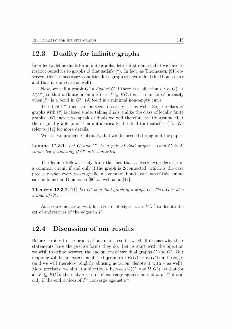
12.3 Duality for infinite graphs 145
12.3 Duality for infinite graphs
In order to define duals for infinite graphs, let us first remark that we have torestrict ourselves to graphs G that satisfy (†). In fact, as Thomassen [91] ob-served, this is a necessary condition for a graph to have a dual (in Thomassen’sand thus in our sense as well).
Now, we call a graph G∗ a dual of G if there is a bijection ∗ : E(G) →E(G∗) so that a (finite or infinite) set F ⊆ E(G) is a circuit of G preciselywhen F ∗ is a bond in G∗. (A bond is a minimal non-empty cut.)
The dual G∗ then can be seen to satisfy (†) as well. So, the class ofgraphs with (†) is closed under taking duals, unlike the class of locally finitegraphs. Whenever we speak of duals we will therefore tacitly assume thatthe original graph (and then automatically the dual too) satisfies (†). Werefer to [11] for more details.
We list two properties of duals, that will be needed throughout the paper.
Lemma 12.3.1. Let G and G∗ be a pair of dual graphs. Then G is 2-connected if and only if G∗ is 2-connected.
The lemma follows easily from the fact that a every two edges lie ina common circuit if and only if the graph is 2-connected, which is the caseprecisely when every two edges lie in a common bond. Variants of this lemmacan be found in Thomassen [90] as well as in [11].
Theorem 12.3.2.[11] Let G∗ be a dual graph of a graph G. Then G is alsoa dual of G∗.
As a convenience we will, for a set F of edges, write V [F ] to denote theset of endvertices of the edges in F .
12.4 Discussion of our results
Before turning to the proofs of our main results, we shall discuss why theirstatements have the precise forms they do. Let us start with the bijectionwe wish to define between the end spaces of two dual graphs G and G∗. Ourmapping will be an extension of the bijection ∗ : E(G)→ E(G∗) on the edges(and we will therefore, slightly abusing notation, denote it with ∗ as well).More precisely, we aim at a bijection ∗ between Ω(G) and Ω(G∗), so that forall F ⊆ E(G), the endvertices of F converge against an end ω of G if andonly if the endvertices of F ∗ converge against ω∗.
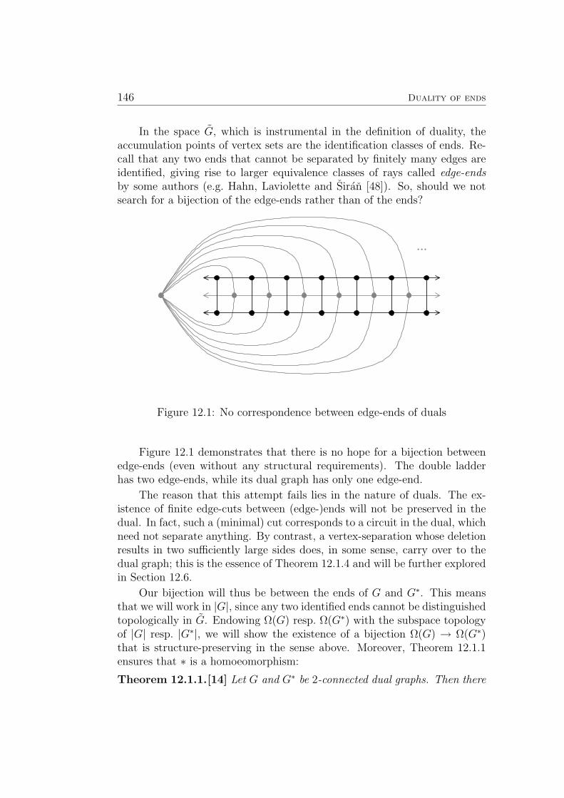
146 Duality of ends
In the space G, which is instrumental in the definition of duality, theaccumulation points of vertex sets are the identification classes of ends. Re-call that any two ends that cannot be separated by finitely many edges areidentified, giving rise to larger equivalence classes of rays called edge-endsby some authors (e.g. Hahn, Laviolette and Siran [48]). So, should we notsearch for a bijection of the edge-ends rather than of the ends?
...
Figure 12.1: No correspondence between edge-ends of duals
Figure 12.1 demonstrates that there is no hope for a bijection betweenedge-ends (even without any structural requirements). The double ladderhas two edge-ends, while its dual graph has only one edge-end.
The reason that this attempt fails lies in the nature of duals. The ex-istence of finite edge-cuts between (edge-)ends will not be preserved in thedual. In fact, such a (minimal) cut corresponds to a circuit in the dual, whichneed not separate anything. By contrast, a vertex-separation whose deletionresults in two sufficiently large sides does, in some sense, carry over to thedual graph; this is the essence of Theorem 12.1.4 and will be further exploredin Section 12.6.
Our bijection will thus be between the ends of G and G∗. This meansthat we will work in |G|, since any two identified ends cannot be distinguishedtopologically in G. Endowing Ω(G) resp. Ω(G∗) with the subspace topologyof |G| resp. |G∗|, we will show the existence of a bijection Ω(G) → Ω(G∗)that is structure-preserving in the sense above. Moreover, Theorem 12.1.1ensures that ∗ is a homoeomorphism:
Theorem 12.1.1.[14] Let G and G∗ be 2-connected dual graphs. Then there
12.4 Discussion of our results 147
is a homeomorphism ∗ : Ω(G) → Ω(G∗), where the two spaces are endowedwith the subspace topology of |G| resp. |G∗|, so that
for all F ⊆ E(G) and ends ω it holds that ω ∈ F if and only if ω∗ ∈ F ∗.(12.1)
We remark that the requirement that G and G∗ are 2-connected cannotbe dropped. This is illustrated by the example of the double ray. Every dualof the double ray is a graph whose edge set is the union of countably manyloops, and thus contains no end at all.
We shall prove Theorem 12.1.1 in the next section.
Let us now turn to our second objective: showing that our bijection ∗preserves thickness. This will be achieved in Theorem 12.1.2. Again, weare confronted with the question why focus on preserving (vertex-)thicknessinstead of “edge-thickness”, i.e. the existence of infinitely many edge-disjointrays in an end.
...
Figure 12.2: Edge-thick end with edge-thin dual end
This is answered by Figure 12.2, which shows a graph that has a singleedge-thick end while the unique end of its dual graph does not even possesstwo edge-disjoint rays. The reason is the same as above: although (or be-cause) the notion of duals is based on edges and operations with edges, theexistence of (small) edge-separators is not preserved in the dual.
Since not all vertex-separators are preserved in the dual, connectivity isnot an invariant of (finite or infinite) duals, as we have already remarked in
148 Duality of ends
the introduction. But, the related notion of Tutte-connectivity is. We deferto Section 12.6 for the definition; suffice it to say here that there are tworeasons why a graph may have low Tutte-connectivity: Either it has a smallvertex-separator or it contains a small circuit. In Section 12.6, we prove thatTutte-connectivity is an invariant of infinite duals, too (Theorem 12.1.4).
Theorem 12.1.4 is an important milestone on our way to proving The-orem 12.1.3 and thus Theorem 12.1.2. Our proof of Theorem 12.1.4 differsfrom the usual proof of Tutte’s finite version, which is done in two steps.First, one shows that Tutte-connectivity coincides with the connectivity ofthe cycle-matroid of the graph. Then one observes that matroid connectivityis invariant under duality.
If we want to use this approach for Theorem 12.1.4 as well, we first haveto answer two questions. Which notion of infinite matroids should we use?And how do we define higher connectivity in a matroid?
The first question is easy to answer. Although it is sometimes claimedthat there is no proper concept of an infinite matroid that provides dual-ity and the existence of bases at the same time, B-matroids, as defined byHiggs [56], accomplish that (see also Oxley [73]). Moreover, one can provethat duality in B-matroids is compatible with taking dual graphs. While thesecond problem, the definition of higher connectivity, can also be overcome ina satisfactory way, its solution together with the introduction of B-matroidswould take quite a bit of time and effort. Therefore, we will, in Section 12.6,present a matroid-free proof of Theorem 12.1.4.
12.5 ∗ induces a homeomorphism on the ends
Before we are able to prove Theorem 12.1.1, we need three lemmas.
The proof of the first of these lemmas is not hard, and also can be foundin [31, Lemma 8.2.2]. We only need the lemma for the proof of Lemma 12.5.2below.
Lemma 12.5.1. Let G be a connected graph, and let U be an infinite subsetof V (G). Then G contains a ray R with infinitely many disjoint R–U pathsor a subdivided star with infinitely many leaves in U .
Lemma 12.5.2. Let G be a 2-connected graph satisfying (†). If U is aninfinite set of vertices then U contains an end of G.
Proof. Suppose otherwise. Then there is no ray R in G with infinitely manydisjoint R–U paths. So, an application of Lemma 12.5.1 yields a subdivided
12.5 ∗ induces a homeomorphism on the ends 149
star S that contains an infinite subset U ′ of U . We delete the centre of S andapply Lemma 12.5.1 again, this time to U ′, which yields another subdividedstar S ′ with infinitely many leaves in U ′. But then, the centre of S and thecentre of S ′ are infinitely connected, contradicting (†).
Lemma 12.5.3. Let G be a 2-connected graph, and let X and Y be twosets of edges such that X ∩ Y ∩ Ω(G) 6= ∅. Then there are infinitely many(edge-)disjoint finite circuits each of which meets both X and Y .
Proof. Let Z be an ⊆-maximal set of finite disjoint circuits so that each C ∈Z meets both X and Y , and suppose that |Z| is finite. Putting Z :=
⋃Z,we pick for every two x, y ∈ V [Z] for which it is possible an x–y path Px,ythat is edge-disjoint from Z. Denote by Z ′ the union of Z with the edge setsof all these paths, and observe that still |Z ′| <∞.
We claim that for every component K of G− V [Z ′] it holds that
for every v, w ∈ N(K) there is a v–w path in (V [Z ′], Z ′ \ Z). (12.2)
Indeed, by construction, there are x, y ∈ V [Z] and (possibly trivial) v–xresp. w–y paths Qv resp. Qw with edges in Z ′\Z. Then x and y are connectedthrough K ∪ Qv ∪ Qw ⊆ G − Z. Hence in Px,y ∪ Qv ∪ Qw ⊆ (V [Z ′], Z ′ \ Z)we find a v–w path. This proves (12.2).
Now, because X ∩ Y contains an end, there exists a component K ofG − V [Z ′] which contains infinitely many vertices of both V [X] and V [Y ].Choose edges eX , eY ∈ E(K) ∪ E(K,G −K) so that eX ∈ X, and eY ∈ Y .Since G is 2-connected, there is a finite circuit C which contains both eX andeY . The maximality of Z implies that C meets Z in at least one edge. Inparticular, C contains the edge sets of (possibly identical) N(K)-paths PXand PY so that eX ∈ E(PX), and eY ∈ E(PY ).
Being connected, K contains a V (PX)–V (PY ) path P . Thus, we find inP ∪PX ∪PY an N(K)-path P ′ with eX , eY ∈ E(P ′). By (12.2), there exists apath R in (V [Z ′], Z ′\Z) between the endvertices of P ′. Now, E(P ′)∪E(R) isa circuit that meets bothX and Y but is edge-disjoint from Z, a contradictionto the maximality of Z.
We can now prove the first main result of this chapter.
Proof of Theorem 12.1.1. We start by claiming that for each F ⊆ E(G) andeach end ω of G the following is true:
if F ∩ Ω(G) = ω then F ∗ contains exactly one end. (12.3)
150 Duality of ends
Suppose the claim is not true. By Lemma 12.5.2, this cannot be becauseF ∗ fails to contain an end; rather there must be (at least) two ends, α1 andα2, in F ∗. Take a finite connected subgraph T of G∗ so that V (T ) separatesα1 and α2 in G∗. For i = 1, 2, denote by Ki the component of G∗ − T towhich αi belongs, and set X∗i := (E(Ki) ∪ E(Ki, T )) ∩ F ∗. Since each ofthe X∗i is infinite, it follows from Lemma 12.5.2 that Xi contains an end.As Xi ⊆ F , this end must be ω. Hence, Lemma 12.5.3 yields disjoint finitecircuits C1, C2, . . . in G each of which meets X1 as well as X2.
We claim that each of the bonds C∗i contains an edge of T . Indeed,let M1 and M2 be the two components of G∗ −C∗i . Since C∗i meets both X∗1and X∗2 , each Mj contains a vertex in K1 ∪ T and a vertex in K2 ∪ T . As,for j = 1, 2, Mj is connected it follows that V (Mj) ∩ V (T ) 6= ∅. So, since Tis connected, there is an M1–M2 edge in E(T ), i.e. C∗i ∩ E(T ) 6= ∅, for eachi ∈ N. This yields a contradiction since the C∗i are disjoint but T is finite.Therefore, Claim (12.3) is established.
Now, we define ∗ : Ω(G) → Ω(G∗). Given an end ω ∈ Ω(G), pick anyset F ⊆ E(G) with F ∩ Ω(G) = ω (choose, for instance, the edge set ofa ray in ω). Define ω∗ = ω∗(F ) to be the, by (12.3), unique end in F ∗.To see that this mapping is well-defined, i.e. that it does not depend on thechoice of F , consider a second set D ⊆ E(G) as above, and observe thatω∗(D) = ω∗(D ∪ F ) = ω∗(F ). Since G is a dual of G∗ (Theorem 12.3.2), wemay apply (12.3) to G∗ and see that ∗ is a bijection and satisfies (12.1).
Next, we prove that ∗ : Ω(G) → Ω(G∗) is continuous. For this, let anend ω∗ ∈ Ω(G∗) and an open neighbourhood U∗ ⊆ Ω(G∗) of ω∗ be given.Then there exists a finite vertex set S ⊆ V (G∗), and a component K ofG∗ − S so that W ∗ := K ∩ Ω(G∗) ⊆ U∗.
Setting F ∗ := E(G∗)\ (E(K)∪E(S,K)), we observe that W ∗ = Ω(G∗)\F ∗. Hence, by (12.1), W = Ω(G) \ F . So, W is an open neighbourhood ofω whose image is contained in U∗. Finally, by interchanging the roles of Gand G∗ we see that the inverse of ∗ is continuous as well.
12.6 Tutte-connectivity
In this and in the next section, we are concerned with how (Tutte-)connectivi-ty is preserved in the dual. The main idea underlying our proofs is the dualityof spanning trees: given a pair of finite connected dual graphs G and G∗, aset D is the edge set of a spanning tree of G, if and only if E(G∗) \D∗ is theedge set of a spanning tree in G∗.
For a pair of infinite graphs, the situation is slightly more complicated.
12.6 Tutte-connectivity 151
In fact, if E(G∗)\D∗ is the edge set of a spanning tree, then (V (G), D) might
very well be disconnected—topologically, however, D (the closure of D in G)is always connected.
Moreover, D forms a topological spanning tree (TST for short) of G: apath-connected circuit-free subspace of G that contains all vertices of G, andevery edge of which it contains an interior point. For more on the relationbetween spanning trees in G and G∗ see [11]. TSTs were first introducedby Diestel and Kuhn in [34], where it is proved that G always has a TSTprovided G is connected.
We will use the tree duality implicitly in the key lemma, Lemma 12.6.4,below. The next two lemmas help to relate the tree duality to vertex sepa-rations.
Lemma 12.6.1. Let G be a graph satisfying (†), let T be a subgraph thatdoes not contain any circuits, and let U ⊆ V (T ) such that 0 < |U | < ∞.Then there exists a set F ⊆ E(T ) of size at most |U | − 1 so that every arc
in T between two vertices in U meets F .
Proof. We use induction on |U |. The assertion is trivial for |U | = 1, so forthe induction step asume that |U | > 1. Choose v ∈ U , then by the inductionassumption there is a set D ⊆ E(T ) such that each vertex w of U \ v lies
in a different path-component Kw of T −D. If there is no vertex w ∈ U \vsuch that v ∈ Kw, we are done, so assume there is such a w.
Observe that there exists exactly one v–w arc A in T − D. Indeed, ifthere were two, then it is easy to see that the edge set of their union wouldcontain a circuit. Now, choose any edge e on A, and set F := D ∪ e.Clearly, F is as desired, which completes the proof.
Lemma 12.6.2. Let H be a connected graph, let F ⊆ E(H), and let W ⊆V (H). If every W -path in H meets F then |F | ≥ |W | − 1.
Proof. Since no two vertices of W can lie in the same component of H − F ,we deduce that H − F has at least |W | components. As each deletion of asingle edge increases the number of components by at most one, H − F canhave at most |F |+ 1 components.
Let us now introduce the notion of Tutte-connectivity, see Tutte [92].For finite graphs, the Tutte-connectivity coincides with the connectivity ofthe cycle-matroid of the graph. We remark that for k ∈ 2, 3, a graph isk-Tutte-connected if and only if it is k-connected. For greater k the twonotions of connectivity are not equivalent.
152 Duality of ends
Definition 12.6.3. A k-Tutte-separation of a graph G is a partition (X, Y )of E(G) so that |X|, |Y | ≥ k and so that at most k vertices of G are incidentwith edges in both of X and Y .We say that a graph G is k-Tutte-connected if G has no `-Tutte-separationfor any ` < k.
Consider a k-Tutte-separation (X, Y ) in a (2-connected) graph G witha dual G∗. To prove that Tutte-connectivity is invariant under taking duals,we would ideally like to see that (X∗, Y ∗) is a k-Tutte-separation in G∗.This, however, is not always true—if the two sides of the separation do notinduce connected subgraphs of G∗, then the number of vertices in V [X∗] ∩V [Y ∗] can be much higher than k. Thus we will strengthen the requirementsand lessen our expectations. By demanding the subgraph (V [Y ], Y )− V [X]to be connected, we shall be able to guarantee that at least (V [Y ∗], Y ∗) isconnected. Moreover, we will be content with finding an `-Tutte-separationof G∗ for some ` ≤ k that is derived from (X∗, Y ∗).
The statement of the next lemma, which accomplishes just that, is abit more general than we need for Theorem 12.1.4, as we shall reuse it forTheorem 12.1.3.
Lemma 12.6.4. Let G and G∗ be a pair of 2-connected dual graphs, and let(X, Y ) be a k-Tutte-separation such that CY := (V [Y ], Y ) − V [X] is non-empty and connected, and such that Y = E(CY ) ∪ E(CY , V [X]). Then
(i) there exists a component L of (V [X∗], X∗) so that (E(L), E(G∗)\E(L))is an `-Tutte-separation for some ` ≤ k; and
(ii) for each component K of (V [X∗], X∗) with |E(K)| ≥ k it holds that(E(K), E(G∗) \ E(K)) is a k-Tutte-separation.
Proof. First, we prove that
Y ∗ is path-connected in G∗. (12.4)
Suppose that this is not the case. Then we can write Y as the disjoint unionof two sets Y1 and Y2 so that there is no Y ∗1 –Y ∗2 arc in G∗ that only usesedges from Y ∗.
In particular, there is no circle in G∗ that only uses edges from Y ∗ andmeets both Y ∗1 and Y ∗2 . Equivalently, there is no bond in G that only usesedges from Y , and meets both Y1 and Y2.
However, since CY is connected and since every edge in Y is incidentwith a vertex in CY , there is a vertex x ∈ V (CY ) which is incident with both
12.6 Tutte-connectivity 153
Y1 and Y2. Observe that the cut Bx of G, which consists of all edges incidentwith x, is a subset of Y . As G is 2-connected, Bx is a bond, which yields thedesired contradiction and thus proves (12.4).
Now, set U := V [X] ∩ V [Y ] and W := V [X∗] ∩ V [Y ∗]. Observe thateach vertex in W is incident with both X∗ and Y ∗. So, if |W | is infinite, thenLemma 12.5.2 implies that X∗ ∩ Y ∗ contains an end, while X ∩ Y does not(as X and Y are finitely separated by U). This contradicts Theorem 12.1.1.We have thus shown that
|W | is finite. (12.5)
Let TX be the edge set of a maximal topological spanning forest of X,i.e. the union of TSTs of the spaces C corresponding to the components Cof (V [X], X). We point out that every circuit of G that lies entirely in X isa circuit of (V [X], X). It follows that TX does not contain any circuits of G.
Next, we prove that
every W -path in (V [X∗], X∗) meets T ∗X . (12.6)
Suppose there is a W -path whose edge set D∗ lies in X∗ \T ∗X . By (12.4),there is a circuit C∗ of G∗ with C∗ ∩ X∗ = D∗. Thus, C is a bond in G,and hence D is a finite cut of the subgraph (V [X], X) of G. Consequently,D contains a bond B of (V [X], X), which then is completely contained ina component KB of (V [X], X). As B ⊆ D ⊆ X \ TX , the intersection ofB with TX is empty. Thus, B is a finite cut of KB that is disjoint fromTX but that separates two vertices incident with TX . Since, on the otherhand, TX restricted to KB is path-connected, we obtain a contradiction.This proves (12.6).
Next, Lemma 12.6.1 yields a set F ⊆ TX of at most |U | − 1 edges so
that every U -arc in TX ⊆ X meets F . This means that every circuit C of Gwith C ∩X ⊆ TX meets F . Thus, every bond B∗ of G∗ with B∗ ∩X∗ ⊆ T ∗Xmeets F ∗. Hence, denoting by K the set of components of (V [X∗], X∗), weobtain that
for every K ∈ K, the graph HK := K − (T ∗X \ F ∗) is connected. (12.7)
Now, for every K ∈ K, observe that by (12.6), every W -path in HK
meets F ∗. So, by (12.7), we may apply Lemma 12.6.2 to HK . Doing sofor each K ∈ K, we obtain that |F ∗| ≥ |W | − |K|. On the other hand,|F ∗| = |F | ≤ |U | − 1 by the choice of F , implying that
|W | ≤ |U |+ |K| − 1. (12.8)
154 Duality of ends
Suppose that for every K ∈ K, it holds that |V (K) ∩ W | > |E(K)|.Then
|W | =∑K∈K
|V (K) ∩W | ≥∑K∈K
(|E(K)|+ 1) = |X∗|+ |K|.
As |X∗| = |X| ≥ |U |, we obtain that |W | ≥ |U | + |K|. This yields a con-tradiction to (12.8), since by (12.5), |W | is finite. Therefore, there exists anL ∈ K with
` := |V (L) ∩W | ≤ |E(L)|.Observe that if we can show now that ` ≤ k, then it follows that
(E(L), E(G∗)\E(L)) is an `-Tutte-separation of G∗, as desired for (i). So, inorder to prove (i), and (ii), it suffices to prove that for each K ∈ K it holdsthat
|V (K) ∩W | ≤ |U |.Suppose otherwise. Then there exists an M ∈ K such that
|W | =∑K∈K
|V (K) ∩W | ≥ (|U |+ 1) +∑
K∈K,K 6=M
|V (K) ∩W |.
Because G is 2-connected, so is G∗ (Lemma 12.3.1). Thus |V (K) ∩W | ≥ 1for every K ∈ K, resulting again in |W | ≥ |U | + |K|, a contradiction, asdesired.
We now prove that Tutte-connectivity is invariant under taking duals.
Proof of Theorem 12.1.4. We show that ifG has a k-Tutte-separation (X, Y ),then G∗ has an `-Tutte-separation for some ` ≤ k. By Theorem 12.3.2, thisis enough to prove the theorem.
First, assume that V [Y ]\V [X] 6= ∅. LetK be a component of (V [Y ], Y )−V [X], and set Z := E(K)∪E(K,G−K). As E(K,G−K) contains at leastone edge for each vertex in N(K), it follows that |Z| ≥ |N(K)|. Thus,(Z,E(G) \ Z) is a k′-Tutte-separation of G for k′ := |N(K)| ≤ k. We cannow apply Lemma 12.6.4 (i) to obtain the desired `-Tutte-separation of G∗.
So, we may assume that V [Y ] \ V [X] = ∅. Then, since |Y | ≥ k, there isa circuit C in Y , say of length ` ≤ k. Hence, C∗ is a bond of size ` in G∗; letK1 and K2 be the components of G∗ − C∗. Now,
|E(K1 ∪K2)| = |X∗|+ |Y ∗| − |C∗| ≥ 2k − `.Thus, we can partition C∗ into C∗1 and C∗2 so that each Z∗i := E(Ki) ∪ C∗ihas cardinality at least `.
12.7 The dual preserves the end degrees 155
In order to show that (Z∗1 , Z∗2) is an `-Tutte-separation of G∗ it remains
to check that U := V [Z∗1 ] ∩ V [Z∗2 ] has cardinality at most `. To this end,consider a vertex v ∈ U , and let j be such that v ∈ V (Kj). Then v is incidentwith an edge e∗v ∈ C∗3−j, whose other endvertex lies in K3−j, because C∗ is acut. This defines an injection from U → C∗, which implies |U | ≤ |C∗| ≤ `,as desired.
12.7 The dual preserves the end degrees
In this section we will use Lemma 12.6.4 in order to prove Theorem 12.1.3that relates the ‘degree’ of an end ω to the degree of its dual end ω∗. Let usfirst discuss the degree notion.
For an end ω, define m(ω) to be the supremum of the cardinalities of setsof disjoint rays in ω; Halin [49] showed that this supremum is indeed attained.In [17] and in [86] the number of vertex- (or edge-)disjoint rays in an endhas been successfully used to serve as the degree of an end in a locally finitegraph (whether vertex- or edge-disjoint rays should be considered depends onthe application). This motivates the definition of the degree d(ω) := m(ω)of an end ω of a locally finite graph.
Now, if G and G∗ are a dual pair of 2-connected locally finite graphs,then it will turn out that m(ω) = m(ω∗) for every end ω of G. In non-locallyfinite graphs we need to be a bit more careful: Figure 12.2 indicates thatdominating vertices should be taken into account.
For an end ω ∈ Ω(G) and a finite vertex set S, we say that U ⊆ V (G)separates S from ω if U meets every ray in ω that starts in S. We define herethe degree d(ω) of an end ω ∈ Ω(G) to be the minimal number k such that foreach finite set S ⊆ V (G), we can separate S from ω in G by deleting at most kvertices from G. If there is no such k, we set d(ω) :=∞. Lemma 12.7.1 willshow that this definition is consistent with the one given above for locallyfinite graphs.
So, denote by dom(ω) the number of vertices that dominate an end ω(possibly infinite). Note that the graphs we are interested in, namely thosethat satisfy (†), are such that dom(ω) ∈ 0, 1 for every end ω.
Lemma 12.7.1. Let G be a graph and let ω ∈ Ω(G). Then d(ω) = m(ω) +dom(ω).
Proof. It is easy to see that d(ω) is at least m(ω) + dom(ω). For the otherdirection, we may assume that dom(ω) <∞. Denote by D the set of vertices
156 Duality of ends
that dominate ω. As D is a finite set, there is an obvious bijection betweenthe ends of G−D and G, which we will tacitly use.
We observe first that for any finite vertex set T , there exists a finite T–ωseparator T ′ in G − D that is contained in CG−D(T, ω). Indeed, otherwise,by Menger’s theorem3, G[T ∪ C(T, ω)] − D contains infinitely many pathsbetween T and some ray in ω that are pairwise disjoint except possibly in T .As T is finite, this implies that T \D contains a vertex which dominates ω,contradicting our choice of D.
Now, choose any finite S ⊆ V (G). Starting with S0 := S \ D we canchoose inductively finite vertex sets Si so that Si ⊆ V (CG−D(Si−1, ω)) is anSi−1–ω separator in G−D, and has minimal cardinality with that property.Since Si ⊆ V (CG−D(Si−1, ω)), all the Si are pairwise disjoint.
Applying Menger’s theorem repeatedly between Si−1 and Si we obtain aset R of disjoint rays in ω of cardinality at least |S1|. As S1 ∪D separates Sfrom ω in G, we have shown that S can be separated from ω by at most|S1|+ |D| ≤ m(ω) + dom(ω) vertices, thus proving the lemma.
We remark that Lemma 12.7.1 can be obtained easily from results ofPolat [76]; we chose to provide the proof nevertheless since the statement ofPolat’s results together with the necessary adaptions would have taken aboutas much time and space.
We finally turn to the proof of Theorem 12.1.3, which asserts that the de-gree of an end is preserved by taking duals. In conjunction with Lemma 12.7.1the theorem immediately yields Theorem 12.1.2.
Proof of Theorem 12.1.3. First assume that d(ω) ≤ k, where k ∈ N is a finitenumber. We wish to show that ω∗ has vertex-degree ≤ k, too.
So, let a finite vertex set T ⊆ V (G∗) be given. Pick a finite edge set F ∗ ofcardinality at least k so that T ⊆ V [F ∗] and so that F ∗ induces a connectedgraph. Now, since d(ω) ≤ k there is a set U ⊆ V (G) of cardinality at most kthat separates (the finite set) V [F ] from ω. If C is the component of G−U towhich ω belongs then set Y := E(C)∪E(C,U) and X := E(G)\Y . Becausek ≥ |U | = |V [X]∩V [Y ]|, and because |Y | =∞ and |X| ≥ |F | ≥ k, it followsthat (X, Y ) is a k-Tutte-separation.
Since F ∗ ⊆ X∗ induces a connected subgraph, there is a component K of(V [X∗], X∗) that contains all of F ∗. As |F ∗| ≥ k, Lemma 12.6.4 (ii) impliesthat (E(K), E(G∗) \ E(K)) is a k-Tutte-separation. Moreover, as ω /∈ X, it
3We use here, and below, that the cardinality version of Menger’s theorem holds ininfinite graphs. This can easily be deduced from Menger’s theorem for finite graphs, seefor instance [31, Section 8.4]

12.7 The dual preserves the end degrees 157
follows that ω∗ /∈ K. Thus, NG∗(G∗ −K) is a vertex set of cardinality ≤ k
that separates T ⊆ V [F ∗] from ω∗, as desired.
In conclusion, since G is also a dual of G∗ (Theorem 12.3.2), it followsthat d(ω) = d(ω∗) if either of ω and ω∗ has finite degree. In the remainingcase, we trivially have d(ω) =∞ = d(ω∗).

158 Duality of ends
Bibliography
[1] M. Ajtai, J. Komlos, and E. Szemeredi. On a conjecture of Loebl. InProc. of the 7th International Conference on Graph Theory, Combina-torics, and Algorithms, pages 1135–1146, Wiley, New York, 1995.
[2] F. Barahona and A. R. Mahjoub. Compositions of graphs and polyhedraII: stable sets. SIAM J. Discrete Math., 7:359–371, 1994.
[3] O. Barr and R. Johansson. Another Note on the Loebl–Komlos–SosConjecture. Research reports no. 22, (1997), Umea University, Sweden.
[4] C. Bazgan, H. Li, and M. Wozniak. On the Loebl-Komlos-Sos conjecture.J. Graph Theory, 34:269–276, 2000.
[5] B. Bollobas. Extremal Graph Theory. Academic Press London, 1978.
[6] B. Bollobas, D. L. Goldsmith, and D. R. Woodall. Indestructive dele-tions of edges from graphs. J. Comb. Theory, Ser. B, pages 263–275,1981.
[7] M. Boulala and J.P. Uhry. Polytope des independants d’un graphe serie-parallele. Disc. Math., 27:225–243, 1979.
[8] S. Brandt and E. Dobson. The Erdos–Sos conjecture for graphs of girth5. Discr. Math., 150:411–414, 1996.
[9] H. Bruhn. The cycle space of a 3-connected locally finite graph is gen-erated by its finite and infinite peripheral circuits. J. Combin. TheoryB, 92:235–256, 2004.
[10] H. Bruhn and E. Berger. Eulerian edge sets in locally finite graphs.Preprint 2008.
[11] H. Bruhn and R. Diestel. Duality in infinite graphs. Comb., Probab.Comput., 15:75–90, 2006.
159
160 Bibliography
[12] H. Bruhn, R. Diestel, and M. Stein. Cycle-cocycle partitions and faithfulcycle covers for locally finite graphs. J. Graph Theory, 50:150–161, 2005.
[13] H. Bruhn and M. Stein. Colouring and characterising claw-free t-perfectgraphs. Preprint 2008.
[14] H. Bruhn and M. Stein. Duality of ends. Accepted for publication inComb., Prob. and Comp.
[15] H. Bruhn and M. Stein. t-perfection is always strong in claw-free graphs.Preprint 2009.
[16] H. Bruhn and M. Stein. MacLane’s planarity criterion for locally finitegraphs. J. Combin. Theory B, 96:225–239, 2006.
[17] H. Bruhn and M. Stein. On end degrees and infinite circuits in locallyfinite graphs. Combinatorica, 27:269–291, 2007.
[18] M.-C. Cai. A remark on the number of vertices of degree k in a minimallyk-edge-connected graph. Discrete Math., 104(3):221–226, 1992.
[19] M.-C. Cai. The number of vertices of degree in a minimally -edge-connected graph. J. Comb. Theory, Ser. B, 58(2):225–239, 1993.
[20] D. Cao and G.L. Nemhauser. Polyhedral characterizations and perfec-tion of line graphs. Disc. Appl. Maths., 81:141–154, 1998.
[21] G. Chartrand, A. Kaugars, and D. Lick. Critically n-connected graphs.Proc. Am. Math. Soc., 32:63–68, 1972.
[22] M. Chudnovsky and A. Ovetsky. Coloring quasi-line graphs. J. Combin.Theory B, 54:41–50, 2007.
[23] M. Chudnovsky, N. Robertson, P. Seymour, and R. Thomas. The strongperfect graph theorem. Annals of Mathematics, 164:51–229, 2006.
[24] M. Chudnovsky and P. Seymour. The structure of claw-free graphs.Preprint.
[25] V. Chvatal. On certain polytopes associated with graphs. J. Combin.Theory B, 18:138–154, 1975.
[26] W. Cook. A minimal totally dual integral defining system for the b-matching polyhedron. SIAM J. Discrete Math., 4:212–220, 1983.
Bibliography 161
[27] O. Cooley. Proof of the Loebl-Komlos-Sos conjecture for large, densegraphs. Preprint 2008.
[28] J. Czipszer, P. Erdos, and A. Hajnal. Some extremal problems on infinitegraphs. Publ. Math. Inst. Hung. Acad. Sci., Ser. A, 7:441–457, 1962.
[29] R. Diestel. Locally finite graphs with ends: a topological approach.Preprint 2009 (Hamburger Beitrage zur Mathematik).Note: A part of this survey will appear in Discr. Math.’s special issue oninfinite graphs, another part in C. Thomassen’s birthday volume (alsoDiscr. Math.).
[30] R. Diestel. The cycle space of an infinite graph. Comb., Probab. Comput.,14:59–79, 2005.
[31] R. Diestel. Graph Theory (3rd edition). Springer-Verlag, 2005.
[32] R. Diestel and D. Kuhn. On infinite cycles I. Combinatorica, 24:69–89,2004.
[33] R. Diestel and D. Kuhn. On infinite cycles II. Combinatorica, 24:91–116,2004.
[34] R. Diestel and D. Kuhn. Topological paths, cycles and spanning treesin infinite graphs. Europ. J. Combinatorics, 25:835–862, 2004.
[35] J. Edmonds. Maximum matching and a polyhedron with 0, 1-vertices.J. Res. Natl. Bur. Stand., Sect. B, 69:125–130, 1965.
[36] F. Eisenbrand, G. Oriolo, G. Stauffer, and P. Ventura. The stable setpolytope of quasi-line graphs. Combinatorica, 28:45–67, 2008.
[37] P. Erdos, Z. Furedi, M. Loebl, and V. T. Sos. Discrepency of trees.Studia sci. Math. Hungar., 30(1-2):47–57, 1995.
[38] J. Fonlupt and J.P. Uhry. Transformations which preserve perfectnessand h-perfectness of graphs. Ann. Disc. Math., 16:83–95, 1982.
[39] A. Frank. Connectivity and network flows. In Handbook of Combina-torics, Vol. 1, pages 111–177. Elsevier, Amsterdam, 1996.
[40] D.R. Fulkerson. Blocking and anti-blocking pairs of polyhedra. Math.Programming, 1:168–194, 1971.
[41] D.R. Fulkerson. Anti-blocking polyhedra. J. Combin. Theory B, 12:50–71, 1972.
162 Bibliography
[42] A. Galluccio and A. Sassano. The rank facets of the stable set polytopefor claw-free graphs. J. Combin. Theory B, 69:1–38, 1997.
[43] A.M.H. Gerards. personal communication.
[44] A.M.H. Gerards. A min-max relation for stable sets in graphs with noodd-K4. J. Combin. Theory B, 47:330–348, 1989.
[45] A.M.H. Gerards and F.B. Shepherd. The graphs with all subgraps t-perfect. SIAM J. Discrete Math., 11:524–545, 1998.
[46] D. Gijswijt and A. Schrijver. On the b-stable set polytope of graphswithout bad K4. SIAM J. Discrete Math., 16:511–516, 2003.
[47] R. L. Graham, B. L. Rothschild, and J. H. Spencer. Ramsey Theory.Wiley, New York, 1990.
[48] G. Hahn, F. Laviolette, and J. Siran. Edge-ends in countable graphs.J. Combin. Theory B, 70:225–244, 1997.
[49] R. Halin. Uber die Maximalzahl fremder unendlicher Wege in Graphen.Math. Nachr., 30:63–85, 1965.
[50] R. Halin. A theorem on n-connected graphs. J. Combin. Theory, 7:150–154, 1969.
[51] R. Halin. Unendliche minimale n-fach zusammenhangende Graphen.Abh. Math. Sem. Univ. Hamburg, 36:75–88, 1971.
[52] Y. O. Hamidoune. On critically k-connected graphs. 32:257–262, 1980.
[53] F. Harary. Graph Theory. Addison Wesley, 1972.
[54] P. Haxell, T. Luczak, and P. Tingley. Ramsey numbers for trees of smallmaximum degree. Combinatorica, 22(2):287–320, 2002.
[55] P. Hell and J. Nesetril. Graphs and Homomorphisms. Oxford UniversityPress, Oxford, 2004.
[56] D.A. Higgs. Matroids and duality. Colloq. Math., 20:215–220, 1969.
[57] J. Hladky and D. Piguet. Loebl–Komlos–Sos conjecture: dense case.Preprint 2008.
Bibliography 163
[58] J. Komlos and M. Simonovits. Szemeredi’s regularity lemma and itsapplications in graph theory. In Paul Erdos is eighty, (Keszthely, 1993),volume 2 of Bolyai Soc. Math. Stud., pages 295–352, Budapest, 1996.Janos Bolyai Math. Soc.
[59] B. Kron and E. Teufl. Ends – Group-theoretical and topological aspects.Preprint 2009.
[60] D. R. Lick. Minimally n-line connected graphs. J. Reine Angew. Math.,252:178–182, 1972.
[61] L. Lovasz. A note on factor-critical graphs. Studia Scientiarum Mathe-maticum Hungarica, 7:279–280, 1972.
[62] W. Mader. uber den Zusammenhang symmetrischer Graphen. Archivder Math., 21:331–336, 1970.
[63] W. Mader. Eine Eigenschaft der Atome endlicher Graphen. Arch. Math.,22:333–336, 1971.
[64] W. Mader. Minimale n-fach zusammenhangende Graphen. 191:21–28,1971.
[65] W. Mader. Ecken vom Grad n in minimalen n-fach zusammenhangendenGraphen. Arch. Math. (Basel), 23:219–224, 1972.
[66] W. Mader. Existenz n-fach zusammenhangender Teilgraphen inGraphen mit genugend hoher Kantendichte. Abh. Math. Sem. Univ.Hamburg, 37:86–97, 1972.
[67] W. Mader. Uber minimale, unendliche n-fach zusammenhangendeGraphen und ein Extremalproblem. Arch. Math. (Basel), 23:553–560,1972.
[68] W. Mader. Kantendisjunkte Wege in Graphen. Monatshefte fur Math-ematik, 78:395–404, 1974.
[69] W. Mader. Kritisch n-fach kantenzusammenhangende Graphen. J. Com-bin. Theory B, 40:152–158, 1986.
[70] W. Mader. On vertices of degree n in minimally n-edge-connectedgraphs. Combinatorics, Probability & Computing, 4:81–95, 1995.
[71] A. R. Mahjoub. On the stable set polytope of a series-parallel graph.Math. Programming, 40:53–57, 1988.
164 Bibliography
[72] A. Sebo. personal communication.
[73] J. Oxley. Infinite matroids. In N. White, editor, Matroid applications,volume 40 of Encycl. Math. Appl., pages 73–90. Cambridge UniversityPress, 1992.
[74] D. Piguet and M. Stein. An approximate version of the Loebl–Komlos–Sos conjecture. Submitted (arXiv:0708.3355v1).
[75] D. Piguet and M. Stein. The Loebl–Komlos–Sos conjecture for trees ofdiameter 5 and other special cases. Electr. J. of Comb., 15:R106, 2008.
[76] N. Polat. A Mengerian theorem for infinite graphs with ideal points.J. Combin. Theory B, 51:248–255, 1991.
[77] W. Pulleyblank and J. Edmonds. Facets of 1-matching polyhedra. InC. Berge and D. Ray-Chaudhuri, editors, Hypergraph Seminar, pages214–242. Springer, 1974.
[78] J.-F. Sacle and M. Wozniak. A note on the Erdos–Sos conjecture forgraphs without C4. J. Combin. Theory B, 70(2):229–234, 1997.
[79] N. Sbihi and J.P. Uhry. A class of h-perfect graphs. Disc. Math., 51:191–205, 1984.
[80] A. Schrijver. Strong t-perfection of bad-K4-free graphs. SIAM J. Dis-crete Math., 15:403–415, 2002.
[81] A. Schrijver. Combinatorial Optimization. Polyhedra and efficiency.Springer-Verlag, 2003.
[82] M. Stein. Ends of small degree in infinite minimally k-(edge)-connectedgraphs. Preprint 2009.
[83] M. Stein. Extremal infinite graph theory. Preprint 2009.
[84] M. Stein. Ends of graphs. PhD thesis, Universitat Hamburg, 2005.
[85] M. Stein. Arboricity and tree-packing in locally finite graphs. J. Combin.Theory B, 96:302–312, 2006.
[86] M. Stein. Forcing highly connected subgraphs. J. Graph Theory, 54:331–349, 2007.
[87] L. Sun. On the Loebl–Komlos–Sos conjecture. Australas. J. Combin.,37:271–275, 2007.
Bibliography 165
[88] E. Szemeredi. Regular partitions of graphs. Colloques InternationauxC.N.R.S. 260 – Problemes Combinatoires et Theorie des Graphes, Or-say, pages 399–401, 1976.
[89] A.G. Thomason. The extremal function for complete minors. J. Combin.Theory B, 81:318–338, 2001.
[90] C. Thomassen. Planarity and duality of finite and infinite graphs.J. Combin. Theory B, 29:244–271, 1980.
[91] C. Thomassen. Duality of infinite graphs. J. Combin. Theory B, 33:137–160, 1982.
[92] W.T. Tutte. Connectivity in matroids. Can. J. Math., 18:1301–1324,1966.
[93] A. Vella and B. Richter. Cycle spaces in topological spaces. J. GraphTheory, 59(2), 2008.
[94] H. Whitney. Non-separable and planar graphs. Trans. Am. Math. Soc.,34:339–362, 1932.
[95] M. Wozniak. On the Erdos–Sos conjecture. J. Graph Theory, 21(2):229–234, 1996.
[96] Y. Zhao. Proof of the (n/2−n/2−n/2) conjecture for large n. Preprint2008.