Embed Size (px)
Citation preview

Notes on Control with Delay
Christopher Brown and David J. Coomhs
The University of RochesterComputer Science DepartmentRochester, New York 14627
Technical Report 387
August 1991
Abstract
We gather together some introductory and tutorial material on control systems with delay.Delay is especially pernicious in feedback systems, and some form of modeling and predictionis essential to overcome its effects. After a short introduction to tbe issues, we present fourbasic techniques for overcoming delay and compare their performance through simulation.The four techniques are the following.
• Predictive techniques to cancel the delay within the loop.
• Cancel negative feedback to obtain open-loop characteristics.
• Smith prediction, which uses a model of the plant.
• System inversion techniques, which use a model of the controller and the plant.
In each of these techniques, predictive filters can be used to overcome latency by providingapproximate dynamic predictions of waveforms within the system, such as input and controlsignals.
This material is based on work supported by the National Science Foundation under Grants numberedIRI-8920771 and CDA-8822724. The government has certain rights in this material.

•
1 Feedback Control and Delay
We are interested in control systems with delay. Feedback control has several familaradvantages - one important one is the decreased sensitivity of a closed-loop negative feedback system to variations in its parameters. Since the open- and closed-loop systems arenot directly comparable, instead we repeat the familiar argument (cf., e.g., [9]) about thedecreased sensitivity of feedback systems to parametric variation. Clearly in an open loopsystem with plant transfer function G(s) and input and output X(s) and Y(s), the changein the transform of the output due to a parameter variation ~G(s] is clearly
~Y(s) = ~G(s)X(,,). (1)
(2)
For a closed loop system, find Y(s) +~Y(s) by substituting G(s) +~G(s) into the familiarformula Y = XG/(l +GH), assume GH(s) » ~GH(s), and obtain
~G(s)
~Y(s) = (1 +GH(s)h X(s).
Defining the system sensitivity to be the ratio of the percentage change in the systemtransfer function to that of the process transfer function, we see that open loop systemshave sensitivity unity, but closed loop feedback systems have sensitivity 1/(1 +GH(s)), thedenominator of which is usually much greater than one.
We bring up this point here only because one of the schemes we shall examine laterchooses to sacrifice closed-loop advantages in order to deal with delay. Given that ideallywe desire feedback, then why is delay a problem in feedback control systems?
We illustrate with the constant-gain feedback system illustrated in Fig. l(a). Here thetransfer function is simply K /(K + 1), and the response to a step function is a scaled stepfunction. Thus this system tracks the input perfectly. Fig. l(b) shows the same systemwith a delay of T seconds added.
The responses of these systems to a unit step are shown in the next two figures. Notshown is the perfect step function output of height 0.4117 that exactly tracks the inputin the continuous controller, zero delay case. Fig. 2 shows the response of the undelayeddiscrete feedback loop to a step input. The discrete controller has an implicit sample andhold circuit, and this characteristic gives the discrete realization of the controller someof the aspects of delayed control. These qualitative differences motivate the use of theZ transform in discrete system analysis. Thus, discrete systems are often written in themanner of Fig. l(b) with the Laplace transform delay box relabeled as a Z-transform delayof Z-l, indicating the inherent delay implied by stepwise operation. Fig. 3 shows the effectof delay in the continuous version of the controller for K = 0.7, and Fig. 4 shows whathappens when the gain exceeds unity.
The decidedly discontinuous performance of the continuous system in the presence ofdelay requires some explanation. The following paragraphs are stolen from [10]. We havethe following situation, where we let the delay be T seconds and we let the time t varycontinuously upward from O. A step input occurs at time t = O.
y = K
1

I y
./ K
(a)
I y
\.. K ee<
.
(b)
Figure 1: Constant gain feedback system: (a) without delay, (b) with delay.
So that
2r < t < 3r
3r < t < 4r
4r < t < 5r
y= l-K
Y = 1 - (1 - K)K = 1 - K +K 2
y = 1 - (1 - (1- K)K)K = 1 - K +K 2 - K3
1- (-K)ny(n)= 1+K (3)
at the nth step.
The steady state gain for the delayed system (if it stabilizes) is the same as for thecontinuous or discrete delayed system steady-state gain: the exponential term in (3) vanishesif the magnitude of K is less than unity.
One can approach the behavior of the delayed system using Laplace transforms. Thismethod puts the problems caused by delay in terms of the delay of the output signal and thepoles introduced into the system by the delay. (For an introduction to basic concepts suchas "poles", see [9) or any other introduction to control theory.) In the following sections ofthis report we shall investigate different methods for eliminating the unpleasant effects ofthe delay and the poles.
The Laplace transform of the output y(t) given input :t(t) with Laplace transform X(s)is
K -e< K£(y(t)) = Y(s) = 1 ~ X(s) = K X(s).+ e-$'T + en
(4)
In the latter form it can be seen that the characteristic equation is not algebraic, andthat it has an infinite number of closed-loop poles. In fact, the poles are the roots of
2

108 9
"Discrete" -
7654321
0.7 r----,----,---,--.,..-...,..-,--.-----,--,----,
0.65
0.6
0.55
0.5
0.45
0.4
0.35
0.3
0.25
0.2 L.....:._'-----'_---'_---'_--l._-'-_......L_--'-_--'--_....J
o
Figure 2: Output of constant gain feedback system for step input and discrete control withK = 0.7. Continuous control yields a perfect step.
, , , , , , ,"Delay" -- -
r-'
-r- -
~-- L- -- L- -
- -, , I ,
0.7
0.6
0.5
0.4
0.3
0.2
0.1
o-1 o 1 2 3 4 5 6 7 8 9 10
Figure 3: Output of delayed constant gain feedback system with step input, K = 0.7.
3

. . I , , , ,
f- "Unotable" - F-f-
,....r-,....
f- ,...., r-
nnr- ,....
.... L-'- '-
'-'-
'-'-
- '-
, , , , , ,
5
4
3
2
I
o-1
-2
-3
-4-I o 1 2 3 4 5 6 7 8 9 10
Figure 4: Output of delayed constant gain feedback system with step input, K = 1.1.
eOT - -K - Ke>(T±2Tq) q - 0 1 2- - , - , t •••
and so
81" = In K + j(l' ± 21'q), q = 0,1,2...
(5)
(6)
Taking K = 1 gives poles falling along the imaginary axis, spaced by 21'/1", the twoprincipal ones (closest the origin) at ±j(l'/1") representing the fundamental oscillatory frequency of period 21' visible in the output. This unstable system then diverges for K > 1,since poles move over into the right halfplane. The extension of eq. (4) to a system with acontroller (transfer function e), a plant (G) and delay (e- OT
) is
(7)
which we shall see again.
In an actual situation, delay again manifests its presence with oscillations. In a straightforward tracking application with the Rochester robot head, one camera on the head is totrack a moving object. With the camera moving, the spatial positional error of the camera'saxis is calculated using information about the camera's position (obtained from reading backangles from the camera's motors) and the image-coordinate error calculated as the distanceof the target's image from the origin of the image coordinate system. If the time betweenreading the two necessary data (camera position and image position) is an unmodelleddelay, the system performs as shown in Fig. 5.
4

10000 15000 20000 25000 30000 350005000
20 .----....,...---r---,--.....---.,....-----r--...,
15
10
5
o-5
-10
-15
-20
-25 L-_-J..__-L-_----''---_-'-__-'-_--'__--l
o
Figure 5: Tracking a sinusoidally moving target. Delay in calculating camera's true angularposition results in an oscillating error that is superimposed on a generally correct sinusoidalhead motion. Here the head position graph is from direct readout from the motors, and theerror is the target's retinal position measured with vision.
5

I Closed LoopI Open LoopNo Delay basis for comparison more robustDelay output delayed output delayed, poles affect
performance
Table 1: Characteristics of undelayed and delayed systems.
Table 1 sums up these generalities. Compared with open-loop control, a closed loop system can be more resistent to variations in behavior induced by plant parameter variations.Introducting delay into an open loop system simply delays the output, while in a closed loopsystem it can also introduce instability. In the sections that follow we present five differentways to cope with the effects of delay and try to make some comparisions between them.We shall investigate the following techniques. In every case the starting point is a closedloop system with delay, having the output delay and multiple-pole characteristic equationdiscussed ahove.
• Cancel negative feedback - achieve open loop performance, delayed.
• Smith prediction - attain closed loop performance, delayed.
• Signal synthesis adaptive control - attain closed loop performance, undelayed.
• Smith and input prediction - attain closed loop performance, undelayed.
• Predictive techniques to estimate and then predict delayed signals within the loop with perfect prediction, attain closed loop performance, undelayed.
2 Opening the Loop
In studying primate gaze control, Young [17] wanted to explain how smooth pursuitavoided instability if tracking is modeled as a pure negative feedback system. There aretwo problems with this model. First, the error, and thus control, signal is zero whenaccurate tracking is achieved; this should send eye velocity transiently to zero. Second,tracking performance is better than it should be given the delays in the control loop andthe time constants of the processes. His proposal is that the system tracks not the retinalimage, hut a neural signal that corresponds to target motion (in the world).
Robinson [12} describes a mechanism that implements Young's idea: as Robinson says,"if negative feedback bothers you, get rid of it". In the negative feedback system the eyevelocity is fed back and subtracted from the target velocity (with some delay). If the eyeis in the process of tracking, then the target velocity is the sum of the eye velocity (withrespect to the head) and the target's retinal velocity (its velocity with respect to the eye).But the latter is just the error signal resulting from negative feedback. Thus an estimatedtarget velocity signal can be constructed by positively feeding back the commanded eyemotion into the control loop, delayed to arrive a t the proper time to combine with the errorterm produced by negative feedback. This mechanism not only provides a signal based
6

G e-·'"
+kR Y......,/ c e-rr
G
-
Figure 6: Feedback cancellation.
on the target's true motion, but it cancels the negative feedback and thus removes thepossibility of oscillations.
In all our examples we shall have a controller in the loop with the plant. Thus the blockdiagram of the feedback-cancellation idea is shown in Fig. 6. Applying the positive feedbackidea in this context involves constructing a model plant G. If the designer's model of theplant and delay is correct, the system is changed to open-loop, losing all the well-knownadvantages of closed-loop control. Further the open-loop response is in fact delayed. Givenaccurate plant and delay models, the designer can do better, as we shall see.
3 Smith Prediction
Smith prediction [13; 14] is a by-now classical technique, is the basic idea behind mostmodern methods. The treatment in [10] is especially readable. Smith prediction was one ofthe main tools for managing cooperating delayed controls in the simulation studies of theRochester Robot [5; 6; 7].
Smith 's Principle is that the desired output from a controlled system with delay T isthe same as that desired from the delay-free system, only delayed by the delay T. Let thedelay be T, the delay-free series controller be C(.), the desired delay controller be C(.) andthe plant be G(.). The delay-free system transfer function will be
CGl+CG'
The delay system with its desired controller has transfer function
CGe-"
l+CGe-"
But Smith's Principle is
CGe-"
1 +CGe-"
7

R f----y
,/ C Ge- II T
- -
i---+ G e-ot -
Figure 7: Smith prediction control.
This quickly leads to the specification for the controller C in terms of C, G, and e-":
- CC= .
l+CG(l-e ")
This simple principle has spawned a number of related controllers, often arising fromeach other by simple block-diagram manipulation. It is worth noting that Smith did nottake the next step and demand that the output should not be delayed. To take this steprequires either a non-physical or a prescient component in the system, as we shall see.
Fig. 7 shows the Smith predictor as applied to the standard situation we use in thisreport, i.e. with continuous control.
This diagram can be rewritten to show the relation to the feedback cancellation technique (Fig. 8).
Assuming exact estimates of G and T, i.e. that G = G and f = T, then the positivefeedback coming to summation point 51 and the negative feedback coming to summationpoint 51 in Fig. 8 cancel, and removing them from the diagram yields a simplified diagramin which Smith's principle clearly holds - the transfer function is
y CGe-n
Y= l+CG'
simply a delayed version of the undelayed closed-loop transfer function.
To sum up, Smith prediction uses the model of the plant in a negative feedback scheme- the controller controls this model. If the model is good, one gets a delayed version of theclosed-loop control. That is, the transfer function of the delayed system is changed from
CGe"1 +CCe OT
to
8

-I
f-y(1 - 82 C
e-U- G
r----------------------~I II .. ' YOUNG POSITIVE FEEDBACKt !- I
G e-'''' :II II I._---------------_.---_.j---------- iI I SMITH PREDICTIONI II
....., . . . .I G I O-DELAY FEEDBACK, II II IL J
Figure 8: Smith prediction and feedback cancellation.
-o- yC Ge-&1'
-
G '--
Figure 9: Cancellation yields Smith's principle.
9

(8)
(9)
The delayed closed-loop negative feedback is there also, and the hope is that it would tuneup the infelicities in the performance due to inaccurate temporal or parametric (plant)modelling. A result of the delay institutionalized in Smith control is non-zero latency,inducing a steady-state error that can vary depending on the input signal. For positionerror tracking of a constant velocity target the latency would cause a steady-state constantpositional error with the tracker trailing behind the target.
4 Signal Synthesis Adaptive Control
4.1 Background
Primate systems seem to track with zero latency. Dahill and his coworkers [1; 11]propose a scheme called signal synthesis adaptive control to achieve the advantages ofundelayed feedback control with zero latency. As we shall see, this requires predictingthe future, something that control theorists are not fond of doing. The scheme is called"signal synthesis" control because the controller is predicting the input signal. It is called"adaptive" because in the published formulation there was a scheme to switch betweenpredicted signals to keep the prediction in line with reality (if a trajectory velocity curvechanged from square wave to sine wave, for example).
The derivation of this type of control presents us with a powerful technique. In fact.on paper it is possible to achieve many different sorts of control, including cancelling thelatency but leaving the poles, cancelling the poles but leaving the latency, cancelling both,and cancelling both and substituting the effect of an entirely new controller for the existingcontroller C. As described, the technique simply uses an inverse plant. These are hardto engineer, since for a plant consisting of integrators one obtains an inverse consistingof differentiators. Still, we shall see that we can rewrite the resulting inverse plant to berealizable and in fact we shall see it has a close relation to the techniques we have seen sofar.
4.2 Inverting a Delayed Feedback System
As a warm up, let us get some intuition by computing the inverse of our standard delayedfeedback system (Fig. 10(a)). The system is
Y(s) = C(s)G(s)e-O'
l(s)1 +C(s)G(s)e n
The inverse of the system, remembering that Laplace transforms compose by multiplication, is just the reciprocal of this expression:
y-I(S) = 1 + C(s)G(s)e-O'
l(s),C(s)G(s)e 0'
which implies that
1 e$T
y-I(S) = l(s)(C(s)G(s)e 0' + 1) = l(s)(C(s)G(s) + 1).
10
(10)

~ C Gy
e-a-r
-
(a)
Iy-t
1/ C 1/ G err ~... ~ ~ +
Input PositiveFeedforward
Inverses
(b)
Time Lead
Figure 10: A delayed system and its inverse, with inverse characteristics labelled.
Translating the rightmost expression into a block diagram yields Fig. lO(b), in whichcertain characteristic features appear including a predictive (non-physical, non-causal) timeadvance component, inverses of the individual components of the system, and a positivefeed-forward of the input signal.
4.3 The System-inverting Controller
The basic block diagram of the system-inverting controller (SIC) is given in Fig. 11.The block labeled SIG. SYNTH. CTRL. does the work. We need to derive what this blockshould do (i.e. how to char acterlze B(s) in terms of the rest of the system and its desiredfunction). To see how the method goes, let us start by imposing the requirement that wewant to synthesize a zero-latency version of the undelayed closed loop original system. Thistakes us a step beyond Smith prediction since we will now reduce the latency to zero. Wethus want
Y(s) = 1(s).
For this equation to hold, we have (selectively dropping the Laplace transform variables):
Since
CGe- STy = 1 +CGe-ST(1 + B).
CGe- STy = 1 = 1+ CGe .~ (I +B),
11
(11)

I + + Y
~\...,/
CGe-"-
SIG. SYNTE.- CTRL
Figure 11: The signal synthesis controller.
I~y
0 + CGe-'" Y,.I
l+CGe-· r
+
l±¢Ge-'f'Cae ,f'
Figure 12: The signal synthesis controller for zero latency realization of closed-loop control.
Finally,
(12)
In eq. (12), the first term inside the parentheses is the inverse of the system, that is ofthe delayed plant and feedback controller. The second term ( -1) simply cancels the input!In this form the SIC block diagram appears as in Fig. 12.
The transfer function of the SIC producing B(s) can be rewritten (multiply the firstterm in parentheses bye", divide 'Jut, simplify)
e,"r-+1CG '
wh.ich we saw in Section 4.2. Written like this, the SIC block diagram is as shown in Fig. 13.
A last rewriting of this particular system shows that it can be realized without any explicit inversions of the components. Thus it can be implemented with the same componentsthat were used to make the Smith controller, as long as the signal is predictable (Fig. 14).
12

I + C@, -'F Y~ 1+ (;e-u'CO
+
Figure 13: Another realization of the signal synthesis controller for zero latency realizationof closed-loop control.
EJI . +0-~le6T
+
or c .. G r-
+) f--- f--.c e.-'T G
.
Figure 14: Block diagram manipulation yields this realization of the system of Fig. 12 or13.
13
•

This basic technique of writing down the desired transfer function of the system andthen solving for B is clearly quite general. For instance, to synthesize a new delay-freesystem with controller D and plant B, simply invert the existing plant, controller, anddelay and substitute the desired ones as follows.
We want the system response to be
y DB7 = 1 +DB
Using the block diagram defining the SIC (Fig. 11) we equate what the system will doto what we want it to do:
GGe-'~ DB(B + I)( 1+GGe-n) = I( 1 +DB)
Solving for B we get
B = I [ DB ] [1 +GGe-IT
_ 1] .1+ DB GGe IT
(13)
Here again we see the input being Subtracted and the inverse of the unwanted systemcomposed with the desired system (Fig. 15).
Finally, we leave it to the reader to apply this technique to the following problem. Giventhe delayed system
GGe- IT
1 +GGe- IT '
the goal is to remove the latency of the system response but not affect the closed loop poles.That is. the goal is to remove the e- ST in the numerator. Derive that
B = lie" -1),
I.e. the controller cancels the input and sends out an advanced version of it to theexisting (delayed) controller, all of which makes sense intuitively and is rather elegant.
5 Enhancing Smith Prediction with Input Prediction
As we have seen, pure Smith prediction removes the delay-induced poles from the controller but leaves the latency. To remove the latency in the Smith controller, it only remainsto predict the input, as in the SIC.
A step in this direction is taken in [4; 5J, in which an explicit kinematic simulation used topredict the system state, and an optimal (Le. variance-minimizing) filter is used to smooththe position and velocity estimation of the world object. Extended Kalman filters, (linear)Kalman filters, and time-invariant filters were investigated as input estimators. However,in this work the filters were not used in their predictive capacity (Fig. 16).
14

R
-1
DRr+rol'
.~
..... :CONTROLLER
DESIRED PLANT
AND CONTROL
INVERSE OF DELAYED PLANT AND CONTROL
Figure 15: System inversion allows any controller to be substituted for the original.
15

Our goal in the current work is to predict the signal for the purpose of compensating fordelays. The predictor will be placed early in the system, before the Smith predictor. Thepure predictor of the SIC i. an "oracleft usually dismissed as unphysical or noncausal. Inthis section we introduce the idea of a predictive filter to supply the necessary en to removethe Smith predictor's latency. It is standard practice with optimal filtering to use statisticaltechniques to see if the current dynamic model fits the data, and if not to substitute anothermodel [3; 8). This "variable dimension" approach is the predictive filtering equivalent ofthe signal synthesis adaptive control scheme [2].
One example of a system incorporating Smith prediction and signal estimation is shownin Fig. 16.
5.1 The a -/3 filter
Linear dynamical systems with time-invariant coefficients in their state transition andmeasurement equations lead to simpler optimal estimation techniques than are needed forthe time-varying case. The state estimation covariance and filter gain matrices achievesteady-state values that can often be computed in advance. Two common time-invariantsystems are constant-velocity and constant-acceleration systems.
Let us assume a constant velocity model: starting with some initial value, the object'svelocity in LAB evolves through time by process noise of random accelerations, constantduring each sampling interval but independent. With no process noise the velocity is constant; process noise can be used to model unknown maneuverings of a non-constant velocitytarget. The cumulative result of the accelerations can in fact change the object's velocityarbitrarily much, so we model a maneuvering object as one with high process noise. For thiswork we assume position measurements only are available, subject to measurement noise ofconstant covariance. Clearly the more that is known a priori about the motion the betterthe predictions will be. Some sensors or techniques can provide retinal or world velocitymeasurements as well.
Assume the object state (its position and velocity) evolves independently in each of the(X, Y, Z) dimensions. For instance, in the Y dimension, it evolves according to
where
y(k +1) = Fyy(k) +v(k), (14)
(15)F = [1 At]y 0 1
for sampling interval At, error vector v(k), and y = [Y, YV. The equations for the othertwo spatial dimensions are similar, and in fact have identical F matrices. Thus for thecomplete object state x = [X, X, Y,y, Z, .iV, F is a (6 x 6) block-diagonal matrix whoseblocks are identical to F y . The error vector v(k) can be described with a simple covariancestructure: E(v(k)vT(j» = QCkj.
The" - f3 filter for state prediction has the form
i(k + 11k +1) = i(k +11k) +[ //At ] [z(k + 1) - z(k +11k)], (16)
16

S
IC
NOISE NOIS
! LWORI D
A SENSORS. OF
OBJE ~T
E D -0-- ROBOTCONTROL DELAY AND ..., NOIS~
~\.) +" HEAD+ -
--- ........ _... ----- .. _--- ~--------------------------------
I Kde! II Kfast I KINEMATICPLANTMODEL
B C
'--DYNAN
MODEL ALPHA - MODELOBJEC
DELAY BETA I.-SENSORS MODEL
FILTERS
iNOISE
MODEE
Figure 16: Smith prediction with kinematic model, signal smoothing and estimation with0-(3 filter. This system exhibits latency.
17

where i(k + 11k + 1) is an updated estimate of x given z(k + I), the measurement at timek+ 1. Here we assume that z(k+ 1) consists of the three state components (X, Y, Z) (but not(X,Y, t». The state estimate is a weighted sum of a state i(k+llk) predicted from the lastestimate to be Fi(klk) and the innovation, or difference between a predicted measurementand the actual measurement. The predicted measurement £(k+ 11k) is produced by applying(here a trivial) measurement function to the predicted state.
The 0 - {3 filter is a special case of the Kalman filter. For our assumptions, the optimalvalues of 0 and {3 can be derived (see [3], for example) and depend only on the ratio of theprocess noise standard deviation and the measurement noise standard deviation. This ratiois called the object's maneuvering indez ~, and with the piecewise constant process noisewe assume,
and
0=~2 + 8~ - (~ + 4)';~2 + 8~
8(17)
(18){3= ~2+4~-~';~2+8~.
4The state estimation covariances can be found in closed form as well, and are simple functions of 0, {3, and the measurement noise standard deviation.
5.2 The 0 - /3 - 'Y Filter
The 0 - {3 . 'Y filter is like the 0 - {3 filter only based on a uniform acceleration assumption.Thus it makes a quadratic prediction instead of a linear one. Broadly, it tends to be moresensitive to noise but bettter able to predict smoothy varying velocities. Its equation is thefollowing.
x(k + 11k + 1) = x(k + 11k) + [ {3/6.t ] [z(k + 1) - z(k + 11k)], (19)1" / 6.t 2
With the maneuvering index ~ defined as before, the optimal u and {3 for the case thatthe target experiences random small change, in acceleration (random jerks) are the sameas before and the optimal 1" = {32 /0:.
Both the 0 - {3 and 0 - {3 - 1" filters have been implemented as C++ classes, in versionswith uniform and nonuniform timesteps. The nonuniform timestep versions are easy extensions in which the timestep is calculated at each iteration as the difference of the last twotimestamps. Appendix A gives the complete code for the uniform timestep 0: - {3 - 'Y filter.
5.3 Input Prediction
The smoothing effect of the estirr arion process improved the performance of the systemin noise [4; 5J. The predictive version of the filter was not used to try to remove latency,however. The classical Smith predictor can be enhanced with some form of input predictionin order to ameliorate the latency built into Smith's principle
18

)+0- L-..+Y
e-·'"C G
-
~ G e-.-r-
Figure 17: Smith prediction control with input prediction to overcome latency.
The resulting block diagram is shown in Fig. 17.
The predictive element eO' may be realized nonphysically by a "prescience filter" ororacle, by actual prior knowledge ofthe signal, or (approximately) by a predictive filter. Bythe same token, the predictive element in the signal synthesis controller shown in Fig. 14may be realized by any of these mechanisms. In later sections we shall do some experimentalwork to assess the relative efficacy of the resulting controllers.
6 Controller Sensitivity
One of our goals is to determine quantitative performance characteristics of each approach to predictive control. Parametric sensitivity analyses quantify the degradation inperformance of controllers to variation in parameters, and temporal sensitivity analysessimilarly quantify the effects of time delays on the system.
Marshall's book [10] has a readable though terse treatment of one analytic approach tosensitivity that is particularly useful in the design and construction of adaptive controllers.The result is due to Tomovic ([15; 16]). If the parameter of interest is a, then write thesystem transfer function as G(s,a). Then the Laplace transform of the output y(t) isY(s,a) = X(s)G(s,a). We assume that the input x(t) is independent of the parameter a.Tomovic's result follows immediately from the definition of the Laplace transform and isthat
(20)
That is, the Laplace transform of the sensitivity function 8y/8a is the product of theLaplace transform of the input and the partial derivitive of the system transfer function withrespect to a. The utility of this result is that usually the partial derivative of the systemtransfer function with respect to a is very close to the transfer function itself, and can beeasily built physically since it is close to the original system. Cascading this derivativesystem with the original system then yields an output that is the sensitivity function. As ithappens, the original transfer function is a factor of the derivitive function, and it is often
19

G lJyjBa
G(s,a)yx
'a'
'b'
lJyjlJbG
Figure 18: Implementing sensitivity functions with sensitivity points
possible to find nodes within the original system whose value is the remaining factors. Inturn, this means that a duplicate of the original system can be cascaded with output fromthese sensitivity take-out points to yield the derivative (Fig. 18).
The method works for delay-free and delayed systems. For example, for the second ordersystem
rPy dydt2 +a dt +by= x(t),
the transfer function is
(S2 +as + b)
and the sensitivity coefficient with respect to a is
BY e-n
Ba = -sX(s2+ as+bP'
For a system G(s) cascaded with a delay e-n, the output z(t) is a delayed version ofyet), namely yet - T). Then the temporal sensitivity function
c (~:) = -sZ(s)
So the temporal sensitivity function is just the time derivative of the system output. Clearlythis makes sense: if a system is changing rapidly, delay changes can result in large differencesin values, whereas if the system is not changing at all, delays have no effect whatever.
Applying these techniques to the system shown in Fig. 7 is easy. The transfer functionis
Yes) =
20
(21)

(22)
If G is a function of some parameter a, then
~Y(s) = Y(s) [ 1:t" ca - cacrr• ] oG.
Ba G 1+CG +C(Ge-rr - Ge:» Ba
The term in square brackets may be rewritten as (1- I'(a), Note then that all parametersensitivity functions will contain the common term f(s)(l-f(s)). In particular the temporalsensitivity of Smith's method is
(Oil ) o«-: 1c ;;- = X(s)f(s)(l- f(s))-o--'or T e-.-r (23)
Further, it is easy to see that (oe-rr /or)/e-" = -so
These calculations can be extended to the case of sensitivity in the case of mismatchbetween the modeled plant and the real one, and between the modeled delay and the realone [10). As of now we have not been able to duplicate this derivation using Mathematica.There is also an approach that uses perturbation analysis and allows the effects of mismatchto be displayed as a change in the block diagram of the system, which is useful for intuition.
At this point more thought could be given to the analytic treatment of sensitivity. Inparticular there are the following obvious problems.
1. Go to the literature in a more responsible way.
2. Derive the sensitivity functions for signal synthesis or system inverting control (SIC).
3. Compare the parametric and temporal sensitivity of Smith and SIC. This involvesthinking about the problem in the Laplace domain or inverse transforming the sensitivity functions.
4. Understand and carry through the mismatch sensitivity calculations for Both Smithand SIC and compare the two approaches.
Leaving these interesting issues aside for now, we proceed to simulation experiments.
7 Experiments
7.1 Simulator and Example System
To explore the effects of noise and systematic error on the control schemes describedhere we wrote a control system simulator. The user specifies the characteristics of blocksin a system diagram, as well as sample rates, input function, and length of run. Thesystem can be continuous, discrete, or hybrid. A continuous system (or block) is specifiedby its differential equation (a variable step Runga-Kutta method is used for solutions).Discrete components include integrators (with various options of anti-windup, integrationtime, saturating or not, and leak), sample and hold, differentiators, gains, inputs (impulse,
21

step, ramp, cosine, and squarewave), additive noise (uniform or gaussian), summers, andoutput blocks. Each block can induce a delay or achieve a time advance. Continuous blocksin use are an integrator, a leaky integrator, a cascaded integrator and leaky integrator, anda spring, mass, damper system. There are also predictors of several varieties. Currently,there are nonphysical "prescient" oracles that look into the future of their input as well asa - 13 and a - 13 - "y filters - the predictors have a provision to produce noisy predictions inwhich the time to look ahead is noisy. New blocks are easy to add and the functionality ofblocks is easy to change.
Using this tool, the systems illustrated in Figs. 6, 14, and 17 were simulated. Severalexamples were tried, to establish for instance that in the ideal case of perfect modelling boththe Smith and SIC controllers achieved the same effect as the undelayed controller. For thisreport we ran experiments in which noisy predictions (rather, accurate predictions but fornoisy values of the future time) and noisy plant models (simulated simply by adding noiseinto the system). Since this experimental approach is really no substitute for an analyticalunderstanding of what is happening, we limited our experiment to a typical case that hasenough complexity to produce interesting behavior. We chose a PID discrete controllerapplied to a continuous spring, mass, damper system.
The action of this controller acting alone on the system is illustrated, first for a stepinput and then for a "sinusoidal" input (actually lI(t)(1 - cos(tw21r)), with u(t) the unitstep). Figs. 19 and 20 show the response of the system and the necessary control signal toa step input, using a good setting of P,I, and D (0.4, 0.4, and 0.8). Fig. 21 shows the stepresponse of the system for a bad setting of P,I, and D (0.9, 0.4, 0.1). Fig. 22 shows thesinusoidal input. Figs. 23 and 24 show the sinusoidal response of the system for the goodand bad settings, respectively.
7.2 The PID-MSD System in Noise
The goal of these experiments is to compare the performance of three approaches overcoming delay. Each approach depends on a system model, and two approaches use modelsof the input. In the experiments to be described, we concentrate on stochastic errors ratherthan systematic errors. In particular we consider additive error in the output of the controller that we intend to model the effects of parametric mis-estimation of the system. Fortemporal sensitivity, we consider stochastic mis-estimation of the correct delay.
To set a baseline for these experiments, we first consider the performance of the pure PIDcontroller for the MSD (mass, spring, dashpot) system described in the previous section.The system diagram is that of Fig. 25.
Clearly there are many parameters that can be interestingly manipulated in experimentson control systems, and many measurements that can characterize the effects. First, to getsome idea of the effects of delay in the feedback loop, consider the system response inthe case of a delay of 0.4 compared with no delay (besides the inherent one-step discretecontroller delay) (Fig. 26).
For this set of experiments, the sampling rate of the discrete controller is a constant0.1 second. The noise added to the controller output is normally distributed, with a meanof 0.0 and a standard deviation of 0.2. The stochastic time perturbation is calculated as
22

0.8
0.7"pidstep" -
0.6
0.5
0.4
0.3
0.2
0.1
0-2 0 2 4 6 8 10
Figure 19: Output of mass, spring, and dashpot system to step input using (P,I,D) = (0.4,0.4,0.8).
, , , ," goodstepcont" -
-- -- -
-
, ,
9
8
7
6
5
4
3
2
1
o-I
-2 o 2 4 6 8 10
Figure 20: Control signal producing the output of Fig. 19.
23

"pidatep.bad" -1.2
1
0.8
0.6
0.4
0.2
0-2 0 2 4 6 8 10
Figure 21: Output of mass, spring, and dashpot system to step input using (P,I,D) = (0.9,0.4,0.1).
i f\ f\ f\ -eol't._
•,,
-J. <.Io-2
0.2
0.'
o.e
l.t
o.•
1.1
1..
1.'
Figure 22: Sinusoidal referenre input u(l)(1 - COS(t",,21T)), with u(t) the unit step, W = 0.5.This input is used throughout rest of work.
24

1.2
"pidsin" -1
0.8
0.6
0.4
0.2
0-2 0 2 4 6 8 10
Figure 23: Output of mass, spring, and dashpot system to u(t)(l - cos(2 ..wt)) input forw = 0.5 using (P,I,D) = (0.4,0.4,0.8).
1.2"pidsiu" -
1
0.8
0.6
0.4
0.2
0-2 0 2 4 6 8 10
Figure 24: Output of mass, spring, and dashpot system to sinusoidal input using (P,I,D) =(0.9,0.4,0.1).
25

NOISE
ir;0- STOCH. YPID DELAY .- P·LANT
-
INHERENT%-1 DELAY
Figure 25: Perturbations in the PID controller. The controller output has additive noiseand there is mis-estimatior. of the "zero" delay, implemented by stochastic non-zero delayor advance. In fact the delay is one time step, since this is actually a discrete controller we have indicated that inherent delay with the %-1 box.
1.. r----,.---...,....---,----,.---..,...--......,
1.2
Q ••
Q ••
Q ••
C.2
l\, I
f tI
\,,,,,\,,\,
10
-0.2 '-__--'- ~__~ ~ .......__.....J
-2
Figure 26: Zero delay case compared to a constant delay of 0.4 in the feedback loop of thesystem. The delay causes overshoot and a phase lag.
26

1., ,.--...,--.......---.,....__....,.. ,....-__..,
1
0.'
0.'
0.'
0.'
·p1dI1noood· "p1u1M01..- -_.
·p11111Nl..l- ... -
e
10••,-0.2 ':---~----:---"7---~---'----...J-,
Figure 27: The conditions of Fig. 23 shown with the results of noise added to controlleroutput and with noisy signal delay and advance.
-v- f-·T '-0 PID --+ e'f -PLANT ~
Figure 28: The PID MSD system with delay and predictor.
the integral number of ticks that results from rounding a normally distributed variate withmean 0.0 and standard deviation of 0.1. The control input is u(t)(l - cos(21rtw)). Theperformance of the perturbed systems can be compared to that of the basic PID controllerand to noisy versions of the PID controller by the metrics of phase lag and gain (Bodeplots) if the frequency of the input sinusoid is varied. Within a frequency, such metrics asovershoot and the sum of absolute differences of the relevant system state (position) suggesttbemselves.
Fig. 27 shows the system state (position of the mass) under the noisy conditions described above compared with the noiseless case.
7.3 Delay and Simple Prediction
The PJD-MSD system is relatively resistant to delay, but its effects are significant. Oneidea is to insert an estimator-predictor in the loop to cancel the effects of delay. Fig. 28shows the system.
Here the delay is compensated by an O! - {3 filter that estimates and predicts the outputof the controller. Using an O!- {3 - 'Y filter has advantages and disadvantages: the advantages
27

Lt,----.,----...,.----..----......---..-----,
l.'
1.'
0.'
0.'
0.'
c. ,
0., • • 10
Figure 29: The undelayed response (solid line) is perturbed by a delay of 0.3s in the controlloop (dashed line). Using the estimator to predict the control signal reduces the phase lagbut overshoot remains.
are less overshoot, the disadvantage is a longer initialization time (three readings instead oftwo) that can make a significant difference in performance when control is active. Fig. 29shows the zero delay case, the case where delay is 0.3 sec. and no prediction is used, andthe case of 0.3s delay and the prediction is for 0.3 sec. ahead. In this system the predictioneliminates the phase lag of the system induced by the delay, but the overshoot of the outputin the delayed and prediction-compensated systems is similar.
7.4 Open Loop Control
It is difficult to compare the performance of the open-loop control approach to theother methods because this approach calls for an entirely new system design: the open loopcontroller in general looks nothing like the closed loop controller. What we show here issimply the degradation of the performance of the controller whose loop has been openedby positive feedback under the two noise conditions of this section: the standard sinusoidalinput, additive noise of 0.2 in the positive feedback path, and normally distributed stochasticvariation of the delay from its mean of 0.0 with a standard deviation of 0.1. For comparisonwe simply give the noiseless performance, which should be (and in fact is, in our simulation)the same as the output of the PID controlled MSD system with negative feedback disabled.This output is not related to the closed-loop PID-MSD system performance, of course.Fig. 30 gives the system configuration and Fig. 31 the three responses.
As mentioned in Section 2, the process of opening the control loop by positive feedbackdoes not remove the delay, or latency, from the output. As with all our schemes, the solutionis simply to cascade an input predictor with the system.
28

NOISE + + {J
'( TSTOCHDELAY
e-O+
+AR Y\.. C e-·'" G
-
Figure 30: The positive feedback loop-opening system, showing where noise and stochasticdelay were injected.
o. s
-eeeex- ·t:c.noi .... -_.
-eeeeea- ._-
,
, ,..•...... ( .. ,, ,, .'.-
10••,-u L-__--'-__~ -'-__....... '___...J
-a
Figure 31: The open loop PID-MSD system output for u(t)(l - cos(2..wt)) input. Idealoutput is shown along with output with G(O.O, 0.2) noise in the positive feedback loop andG(O.O, 0.1) stochastic delay in the positive feedback loop.
29

R I--Y
,./e-n
C G. -
NOISE{;
+A+ STOCl'!I DELAY -'I
Figure 32: The Smith predictor with noise added to simulate plant and delay mis-modeling.The STOCH. DELAY box represents a stochastic variation about the modelled delay, whichitself is ideally the same as the true plant delay.
Since the open- and closed-loop systems are not directly comparable, we simply invokethe argument of Section 1 concerning the decreased sensitivity of feedback systems to parametric variation. If we can afford to give up the advantages of feedback systems, thenan open-loop controller can of course be used, and then delay will only cause a latencyin output that can be more or less compenstated by predictive filtering somewhere in thesystem.
7.5 Smith and Signal Prediction
The block diagram of the system used in this section is given in Fig. 32. As before, thecontroller is the PID controller of earlier sections and the system is the same mass, spring,damper system.
This system diagram is interesting because it brings up the following question. Supposethat mis-modelling the plant actually is modeled as additive noise emanating from the plantmodel. In the case of zero modelled delay, this noise is both added to and subtracted fromthe error signal, and thus cancels itself completely. This argument extends to any behaviorof the plant model at all, of course: it is all subtracted out in the zero-delay case.
Consider two cases, the zero delay case with noises as we have had previously, and acase in which the plant delay is 0.2, which is accurately reflected in the model delay exceptwhen that modelled delay is perturbed by our standard stochastic perturbations. In thiscase the effect of the noise is doubled, since a shifted version is subtracted from itself at theinput. We obtain the graphs of Figs. 33 and 34. As expected, the Smith predictor avoidsthe deleterious effects of systematic delay (Fig. 26) on the system output, but retains adelay or latency in its output equal to that of the system delay.
30

1.2 I--....,---.-__.,....__...... ~__--,·...nt.!'lcD.at...
.. -.ithcoNlo1 .... -_."--.1tb.::oloCl.l" - ••
o.•
o.•
o••
0.2
•", ,, ,
, :,., .., ,, ,, ", ., '.· "· '., .· ' ., ' ,, ,, ' .. ,. ," ., .. ,, ' ... ,.' ......
....,.,,···,,,,. ,"
102
o-':-2- __~__--: ~__--'~__~__--J
Figure 33: The Smith controller with zero modelled delay. Ideal output is shown (solid line)along with output with G(O.O, 0.2) noise in the feedback loop (long dashes) and G(O.O, 0.1)stochastic delay in the feedback loop (short dashes). The controller cancels the noise in thiscase (see text), so the long dashed line is the same as the solid one.
.,"
1.2
.".,
o.•
c.•
o.•
0.2
0-2
".md.elok" "DllIelno1••- -_.
".IIId.elet_1." ......
.:
,,
1O
Figure 34: As in the previous figure, only with 0.2 system delay, Compared with the lastfigure, note the similarly-shaped, but delayed, ideal output, which is shown along withoutput with G(O,O, 0.2) noise in the feedback loop and G(O.O, 0.1) stochastic delay in thefeedback loop.
31

NOISE
+6-J .... STOCI
ADV. +6:<y C ~ G ...
+) YC I-- e-·'T r- G
-
Figure 35: The SIC realization, with noise added to simulate plant and delay mis-modeling.The STOCH. ADV box represents a stochastic variation about the modelled necessaryadvance, which itself is ideally the same as the true plant delay.
7.6 Signal-Inverting Control
Although this controller is inspired by, and in its most general form (Fig. 15) demandsthe inversion of the following system, here we use the rewriting that merely calls for aduplication of the controller and a model of the plant (along with a nonphysical signaladvancer). Fig. 35 shows the system used in the simulations. Fig. 36 shows the resultswith the standard noise parameters of this section.
8 Input Prediction
In the experiments in Section 7, the Smith and SIC controllers needed to be able topredict the input in order to overcome ali the effects of delay. So far we have assumed anoracle that actually knows the future. This is an impractical general solution (althoughin some cases one can make an argument that very precise expectations are downloadedinto the controller - this is a central idea in the signal synthesis adaptive controller [1;11].
In this section we examine the effectiveness of the Q - Band 0 - {3 - 1 filters for inputprediction. Recall that the former makes linear predictions based on past input and its
32

i • , ,--,---.,....---,---...,...---..---...,
0 ••
f\ "
~i\\ .~ \0.'
" ~I, , 1, , 1
V, ,,, ,
o.•,,
I' ,
e. , 0) '0 Y\.'/
'-0-z • 10
Figure 36: The SIC controller dealing with a delay of 0.4. The delay is not present in theoutput since the (nonphysical) signal advancer presents the controller with its future value,thus removing the delay. The ideal output is shown along with output with G(O.O, 0.2)noise added to the predictive section and G(O.O, 0.1) stochastic advance noise added to thetrue value.
inherent beliefs about the reliability of its sensors versus the predictability of the target.The latter makes quadratic predictions.
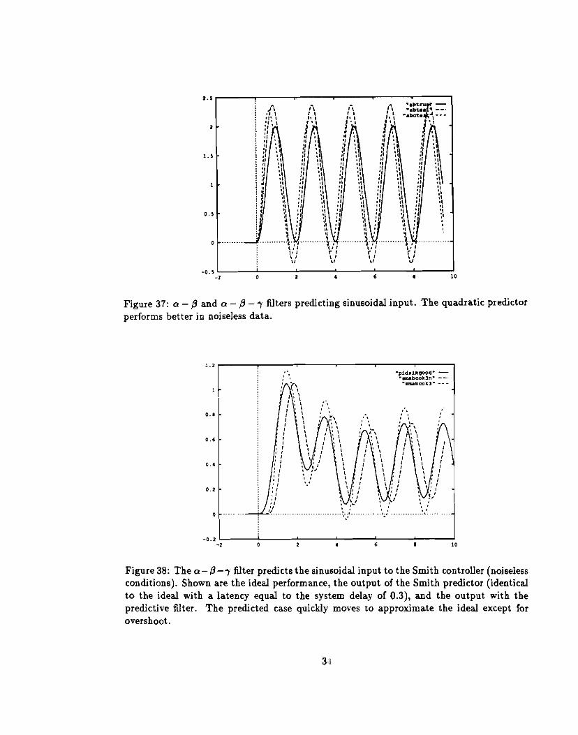
As an example, Fig. 37 shows our standard sinusoidal input u(t)(l - 211'wcos(t)) andthe predicted value for 0.2 seconds into the future yielded by the" - f3 and" - f3 - "I filterswith>. '" 1 (equal confidence in data and prediction). Neither filter's assumptions aboutconstant velocity or acceleration is met. The" - f3 - "I filter delivers reasonable predictionswith less overshoot. The" - f3 filter is rather less satisfactory.
The" - f3 - "I filter may be substituted for the input predictor in the Smith and SICschemes. For the Smith predictor and a delay of 0.3, the results are shown in Fig. 38. Theoutput is close to the ideal output, but shows the characteristic overshoot engendered bythe predictive filter.
When the" - f3 - "I filter is substituted for the input predictor in the SIC scheme, theresults are not quite as good. Fig. 39 shows the ideal and SIC outputs and the correspondingone from the Smith predictor (identical to the predictive filter output of Fig. 38).
A closer approximation to the desired output is actually possible by setting the prediction to 0.4 instead of the correct 0.3. Not only does this change result in less overshoot butin a much closer following of the desired curve between the peaks. This sort of tradeoff isalso noticed in the laboratory, where the delay and >. (maneuvering index) parameters maybe traded off to improve performance.
For noiseless data, the maneuvering index (reflecting our faith in our sensors over thatof our predictions) may be increased. Substantially improved performance results with
33
,.. r---...,....--~~--...,....--....,.---~---,. .. ".bt.ru:r: -1\ 1\ -.btu .. -_.:.\ "1 ...bet.,.",,'--
}' ,' t· I
'I • J . ! ~", " ., I
'I' 'J ., ,:': .:,' ~ t :1 ~ I,I II ,\ 11 . 10'" .1" tI 'I'I" "'I 01',n U :: ~, ;1 !\.1 01 :, .1 ,I .,.\ ., 'I " ., '1°1 'I " 'I '1 "
n ~\ :: ~\ ;: :\II ,I:' ,I ,I .,0' '1 ,I 'I II .,'I '.., '1" "'I '\: I ',: I ~l: ~1 ~I. ,
: ~\ ~: ~"' I '" ' •
···l.I······~,,. I I' Jr I r •,I I j
" "
,.\/ ,,. ,,.,
J •, d •
" '" '~ I :':_.\ ,I ,I'I 01.,'I II 'I~\ 'I ".\ i: :~'I .1 II" '1 IIi' 'I 'I
~ :1 :~'I" .,,\ " 'I:~" ".. ~ I :'II, "" ., ' .,
······1·, /····t:,,l \.,l' , r I\ I \ /\1 I.'
J"',j,·t' \:: ~ I:,"""":,"".,":,,•~,•,
D
,
D••
1..
10••,D
-D.' L '--__--' ...... --'- ...... .J
-a
Figure 37: a - {3 and a - {3 -, filters predicting sinusoidal input. The quadratic predictorperforms better in noiseless data.
1.2 r-----,.---...,---~---......---...,..---..,
", .
~p1d.1n.qooc1" ".,rwlbc:ol!:3n" -_.
"arIIIIDcoll:3" ---
.. _..~.
~\ ' ., ,, ,, I, ,: ,, I,,,,,,,,
, ' r\ ~ I
, I
"", ,. ~_ .•..'.'
,,,,, ,
I ~ \I ' ,I I1 I1 II ,
l \, ,, ,, ,, : 'I, I I, I, I I: I
: I ,,l./, ,• r ' •.,, ,:,,,'I""
e. ,
c.•
0.'
D.•
10•e-0 z L-__~---~---~----:-----:------:'.,
Figure 38: The 0- {3-, filter predicts the sinusoidal input to the Smith controller (noiselessconditions). Shown are the ideal performance, the output of the Smith predictor (identicalto the ideal with a latency equal to the system delay of 0.3), and the output with thepredictive filter. The predicted case quickly moves to approximate the ideal except forovershoot.

"p1ddnvood~ "blylbcl" -_.
"1113" ~--
(\I'.,f '•
•\ . \. . ,\ ~ ~
·_·_-_······~]····_· __ ·_·~f.-.f··_·········~i·----·_···\J \,.,
'.'..fj,
1.2,----;--;:--.--_--, ...,... ..-__--,
o.•
0.2
o ....
0.'
0.'
"•2
-0.2 L.-__--'- -'-__----' ....... "'--__....l-2
Figure 39: The n - {3 - '"I filter predicts the sinusoidal input to the SIC controller (noiselessconditions). Shown are the ideal performance, the output of the SIC controller for the delayof 0.3), and the comparable output of the Smith predictor shown previously.
x= 10.0 (Fig. 40).
9 Discussion
Our goals here were two: understand classical work on control with delay, and apply themost promising techniques in our laboratory to cope with the real delays we experience.
We suspect that there has been more written on delay control that we should read.We feel that mathematical analysis of the systems we have discussed could well be pushedfarther. Our simulator has proven a useful and flexible tool and could support countlessmore experiments by varying parameters of noise, input frequency, delay accuracy, andmismatching of modelled controllers and plants with the real ones.
A summary of our evaluation of several approaches to control of time-delay systems isas follows.
1. Ignore the delay or compensate by lowering controller gains: Infeasible in general, thissolution might work for some applications because of the relatively short delays thatarise with some of our equipment.
2. Opening the loop through positive feedback: This solution does not appeal, since itloses all the advantages of feedback control and seems sensitive to delay.
3. SIC control: Cancelling various parts of the downstream system by inversion is ageneral and powerful. if practically difficult, idea. This approach requires modelling
35

,\. \', \\ I" ,. 'I I -,,'., \ " \ I
._._ ~.I. .······\.I- ..•..········).!···_·_·- .,I '
"p1d.1rlqood- --pl- -_.
---.).10· ---
1.2 ,.,,,,\I.I>I.II
D.'
D.'
D.•
D.2III
'j
,..1 I
".'t·
",
"::.~,."
1\,j »,t',:
10. I•-D.2 l..-__...... -'-__--''-__-:-__....,.-:.-__-;
-2
Figure 40: Ideal performance and the Smith predictor with its o - f3 - "( predictive filterpredicting the sinusoidal input. The performance of the filter with noiseless input data ismuch better with>. = 10 than with>. = 1.
of the controller as well as of the controlled plant. For a software controller that isnot infeasible, but complicates matters somewhat. There are useful cases where itsrealization does not calI for computing the inversion ofthe controlled plant (generallya bad idea because it would calI for differentiators). We have not seen this rewritingof the SIC controller presented elsewhere. The SIC seems slightly more sensitive tonoise and delay mismatches' than does the next scheme, but probably not enough toworry about.
4. Smith with input prediction control: This classical scheme is elegant and has somepractical advantages (not modelling the controller, just the plant).
It is worth mentioning that predictive filters have more uses than predicting the signal:they also estimate the signal. The latter facility is useful when the signal is noisy or dropsout. Our Q- f3 and o - f3 -"( filters continue predicting and estimating until a certain amountof time (a filter parameter) elapses during which the filter sees no input data. We expectthe estimation aspect of the filters to be as useful as their predictive aspect in practicalsituations, since the delays confronting us with the MaxVideo equipment and robot headcamera controllers is relatively small (on the order of 100 ms or less) compared say to thedelays we see with the Puma robot and its VAL controller (on the order of 500 ms).
The filter software described here is used in several laboratory projects and the simulator.We hope that this document and possibly the simulation software we have developed willprove useful for further practical work in the laboratory or at least for helping to understanddelay systems.
36

References
[IJ A. T. Bahill and D. R. Harvey. Open-loop experiments for modeling the humaneye movement system. IEEE Transactions on Systems, Man, and Cybernetics, SMC16(2):24~250, 1986.
[2] A. T. Bahill and J. D. McDonald. Adaptive control models for saccadic and smoothpursuit eye movements. In A. F. Fuchs and W. Becker, editors, Progress in OculomotorResearch. Elsevier, 1981.
[3] Y. Bar-Shalom and T. E. Fortmann. Tracking and Data Association. Academic Press,1988.
[4] C. M. Brown. Kinematic and 3D motion prediction for gaze control. In Proceedings:IEEE Workshop on Interpretation of 3D Scenes, pages 145-151, Austin,TX, November1989.
[5] C. M. Brown. Gaze controls cooperating through prediction. Image and Vision Computing, 8(1):10-17, February 1990.
[6] C. M. Brown. Gaze controls with interactions and delays. IEEE Transactions onSystems, Man, and Cybernetics, in press, IEEE-TSMC20(2):518-527, May 1990.
[7] C. M. Brown. Prediction and cooperation in gaze control. Biological Cybernetics,63:61-70, 1990.
[8] C. M. Brown, H. Durrant-Whyte, J. Leonard, and B. S. Y. Roo. Centralized andnon centralized Kalman filtering techniques for trackingand control. In DARPA ImageUnderstanding Workshop, pages 651-675, May 1989.
[9] Richard C. Dorf. Modern Control Systems. Addison Wesley, 1986.
[10] J. E. Marshall. Control of Time-Delay Systems. Peter Peregrinus Ltd., 1979.
[11] J. D. McDonald and A. T. Bahill. Zero-latency tracking of predictable targets bytime-delay systems. Int. Journal of Control, 38(4):881-893,1983.
[12] D. A. Robinson. Why visuomotor systems don't like negative feedback and how theyavoid it. In M. A. Arbib and A. R. Hanson, editors, Vision, Brain, and CooperativeComputation. MIT Press, 1988.
[13] O. J. M. Smith. Closer control of loops with dead time. Chemical Engg. Proq. Trans.,53(5):217-219,1957.
[14] O. J. M. Smith. Feedback Control Systems. McGraw-Hill, 1958.
[15] R. Tomovic. Sensitivity Analysis of Dynamic Systems. McGraw-Hill, 1963.
[16] R. Tomovic and M. Vukobratovic. General Sensitivity Theory. Elsevier, 1977.
[17] L. R. Young. Pursuit eye movement - what is being pursued? Deo. Neurosei.: Controlof Gaze by Brain Stem Neurons, 1:29-36, 1977.
37

A The Q' - f3 - 'Y Filter in C++
1*************** Header File filt.h ****************1
'ifndef _filt_htdefine _filt_h
1* did we see a target or not on this "tick" ?*Ienum data_type {data, nodata}:
1* what is the filter doing? *1enum filter_activity{1nvalid, initializing, tracking,predicting,timed_out}:
I. this struct is used to set filter characteristics at creation time. *1
typedef struct filter_params{double time_step;
double timeout_secs;int init_ticks:double alpha, beta,gamma;
} .filter_params_t;hndif
I•••••••••• Header File ABC.h *****•••1'ifndef _ABC_htdefina _ABC_h
'include <stream.h>'include "filt .h"
class abcfilter{
protected:filter_params f _params ;int timeout_ticks;double xlast, xcurr. vlast. vcurr. vave; Ilfor the a-b filter calc.double xave, alast, acurr, aave; II for a-b-c calc.double x_pred. v_pred. a_pred. innov: Ilmore intermediate variablesdouble N;
public:filter_activity activicy;
38

double x_est, v_est, a_est; Ilestimated variabledouble x_future, v_future. a_future:Ilpredicted variable at time advance in the future;int age_ticks; II total age;double age_sees; II total age:int data_ticks: Ilhov long ve've seen targetdouble data_sees; Ilhov long ve've seen targetint nodata_ticks; II hov long ve've not seen targetdouble nodata_secs; II hov long ve've not seen target
II all the above are public so user can just inquire ..•
abcfilter(filter_params parms): Ilcreate and initvoid run (data_type signal, double x, double advance); Ilassumes runs every tick.void run(data_type signal, double x. double advance, double timestamp);
II for irregular data arrival
void dump(void);};
lendif
I ••••••••• Filter Code ••••••••••1
'include "ABC.h"
I. Create and Initialize Filter .1
abcfilter::abcfilter( filter_params parms){
int i;
activity. initializing:age_ticks. 0;age_sees. 0.0;data_ticke • 0;data_sece • 0.0;nodata_ticks = 0:nodata_secs • 0.0:timeout_ticks = irint(f_params.timeout_secs/f_params.time_step);
xcurr = vcurr = vave c xave • aave c acurrc 0.0;
39

}
/* irregular timestep version is very similar */
void abcfilter::run(data_type signal, double X. double advance){
activity - (age_ticks < f_params.init_ticks)? initializing: tracking;//tracking or predicting actually, but ve'll find that out later
double adv = advance;
if ( activity == initializing){
if (signal == nodata) {activity= timed_out; return;}//policy decision -- don't initialize through dropout
N • double(age_ticks) + 1.0; //for running average in itialization
/* there follows a segment to initialize the filter .. keeps a runnning ave.of the acceleration, uses latest values for velocity and position .•/
if (age.ticks >= 0){ xlast = xcurr;
xcurr = X;}
if (age_ticks >- 1){vlast z vcurr;vcurr = (xcurr - xlast)/f_params.time_step;
}if (age_ticks >= 2)
{alast c acurr;acurr • (vcurr - vlast)/f_params.time_step;aave - aave + (acurr - aave)/(N-2.0);}
if (age_ticks < 2) activity = invalid;
/* nov compute the estimates and future predictions during initialization */
40

x_est = xcurr;v_est. vcurr;
a_sst = aave;x_future· x_est + v_est*(adv) +
+ 0.5 * a_est * (adv*adv);v_future K v.est + adv*a_8st;
a.future E a_est;
}Ilend initialization phase
else II in this case, ve are actually filtering{
1* start timer if no data .. .*1
if (signal.· nodata) II no data this time .. start predicting blindly{if (nodata_ticks++ >. timeout_ticks){activity. timed_out; return;}activity =predicting;data_ticks = 0;
x_est = x_est + v_est*f_params.time_step+ O.S*a_est*f_params.time_step*f_params.time_step;
Ilpredict based on last known vel, acc ..v_est = v_est + a_est*f_params.time_step; Illast known acc ...}
1* Following are the alpha-beta-gamma equations! *1
if (signal == data) Ilgot data this time, can do the full calculation{activity = tracking;nodata_ticks = 0;data_ticks++;x_pred • x_est + f_params.time_step*v_est+ O.S*a_est*f_params.time_step*f_params.time_step;v_pred = v_est + f_params.time_step*a_est;innov = X - x_pred;Ilcompute the current estimatex_est = x_pred + f_params.alpha*innov;v_est =v_pred + (f_params.beta/f_params.time_step)*innov;
41

a_est • a_est +
(f_params.gamma I (f_params.time_step*f_params.time_step»*innov;
}
II compute the predicted future valuex_future. x_est + v_est*adv + O.5*a_est*adv*adv;
v_future· v_est + adv*a_est;a_future· a_est;
}
age_ticks++; Ilgo to next time stepage_sees +- f_params.time_step; II in real time ...data_sees. data_ticks*f_params.time_step;nodata_secs = nodata_ticks*f_params.time_step;
} II end run
.2