Normalization - German Cancer Research Center · 6/9/2013 3 Normalization of Agilent data in Chipster Background correction • Background treatment None, Subtract, Edwards, Normexp

6/9/2013

1

Normalization

Methods

Affymetrix• Background correction + expression estimation + summarization• RMA (Robust Multichip Averaging) uses only PM probes, fits a model

to them, and gives out expression values after quantile normalization and median polishing

Agilent• Background correction + averaging duplicate spots + normalization

Illumina• Background correction (in GenomeStudio) + normalization

After normalization the expression values are in log2-scale• Hence a fold change of 2 means 4-fold up, -2 means 4-fold down, etc

6/9/2013

2

Normalization of Affymetrix dataPreprocessing = background correction + expression estimation +

summarisation

Methods: MAS5, Plier, RMA, GCRMA, Li-Wong• MAS5 is the older Affymetrix method, Plier is a newer one• RMA is the default, and works rather nicely if you have more than a few chips• GCRMA is similar to RMA, but takes also GC% content into account• Li-Wong is the method implemented in dChip

Variance stabilization makes the variance over all the chips similar• Works only with MAS5 and Plier (the other methods output log2-transformed

data, which is thus corrected for the same phenomenon)

Custom chiptype• Because some of the Affymetrix probe-to-transcript mappings are not correct,

probes have been remapped in the Bioconductor project. To use these remappings (alt CDF environments), select the matching chiptype from the Custom chiptype menu.

Normalization of Agilent dataBackground treatment often generates negative values, which are

coded as missing values after log2-transformation.• Usual subtract option does this• Using normexp + offset 50 will not generate negative values, and it

gives rather good estimates (the best method reported)

Loess removes curvature from the data (suggested)

Before After

6/9/2013

3

Normalization of Agilent data in Chipster

Background correction• Background treatment

None, Subtract, Edwards, Normexp• Background offset

0 or 50

Normalize chips• None, median, loess

Normalize genes (not needed for statistical analysis)• None, scale (to median), quantile

Chiptype• You must give this information in order to use annotation-based tools later

Normalization tools for Illumina data in ChipsterNormalization / Illumina

• Normalization methodNone, scale, quantile, vsn (variance stabilizing normalization)

• Illumina software versionGenomeStudio or BeadStudio3, BeadStudio2, BeadStudio1

• Chiptype• Identifier type

Target ID, Probe ID (for BeadStudio version 3 data)

Normalization / Illumina - Lumi pipeline• Transformation

none, vst (variance stabilizing transformation), log2 • Normalize chips

none, rsn (robust spline normalization), loess, quantile, vsn• Chiptype

human, mouse, rat• Background correction

none, bgAdjust.Affy

6/9/2013

4

Quantile normalization procedure

Sample A Sample B Sample C

Gene 1 20 10 350

Gene 2 100 500 200

Gene 3 300 400 30

Sample A Sample B Sample C Median

Quantile 1 20 10 30 20

Quantile 2 100 400 200 200

Quantile 3 300 500 350 350

Sample A Sample B Sample C Median

Quantile 1 20 20 20 20

Quantile 2 200 200 200 200

Quantile 3 350 350 350 350

Sample A Sample B Sample C

Gene 1 20 20 350

Gene 2 200 350 200

Gene 3 350 200 20

1. Raw data

2. Rank data within sample and calculate median intensity for each row

3. Replace the raw data of each row with its median (or mean) intensity

4. Restore the original gene order

Checking normalization

6/9/2013

5

Exercise 2: Normalize Illumina data

Import folder IlluminaTeratospermiaHuman6v1_BS1 using the Import tool like in exercise 1.

In the workflow view, click on the box ”13 files” to select all of them

Select the tool Normalization / Illumina. Set parameters so that • Illumina software version = BeadStudio1• identifier type = TargetID• chiptype = Human-6v1

Repeat the run as before, but change • Normalization method = none• This ”mock-normalization” gives you unnormalized data that can be used

as a comparison point when looking at the effect of normalization later.

Describing the experimental setup

6/9/2013

6

Phenodata – describing experiment setupExperimental setup is described with a phenodata file, which is created during normalization

Fill in the group column with numbers describing your experimental groups

• e.g. 1 = healthy control, 2 = cancer sample• necessary for the statistical tests to work• note that you can sort a column by clicking on its title

How to describe pairing, replicates, time, etc?

You can add columns to the phenodata file

Time• Use either real time values or recode with group codes

Replicates• All the replicates are coded with the same number

Pairing• Pairs are coded using the same number for each pair

6/9/2013

7

Phenodata for prenormalized data

If you bring in previously created normalized data and phenodata:• Choose ”import directly” in the Import tool• Right click on normalized data, choose ”Link to phenodata”

If you brought in normalized data and need to create phenodata for it:• Use Import tool to bring the data in• Use the tool Normalize / Process prenormalized to create phenodata

• Remember to give the chiptype• Fill in the group column

Exercise 3: Describe the experiment

Double click the phenodata fileIn the phenodata editor, enter 1 in the group column for the control samples and 2 for the teratospermia samples.

6/9/2013

8

Quality control (inc. clustering theory)

Quality control tools

Quality control• Affymetrix basic (RNA degradation + Affy QC)• Affymetrix RLE (relative log expression) and NUSE (normalized

unscaled standard error plot) fit a model to expression values• Illumina (density plot + boxplot)• Agilent 2-color (MA-plot + density plot + boxplot)• Agilent 1-color (density plot + boxplot)

Visualization• Dendrogram• Correlogram

Statistics• Non-metric multidimensional scaling (NMDS)• Principal components analysis (PCA)

6/9/2013

9

Affymetrix

Quality control information• Affymetrix QC metrix• RNA degradation• Spike-in controls linearity• RLE (relative log expression)• NUSE (normalized unscaled standard error plot)

Visualization• Dendrogram• Correlogram

Statistics• Non-metric multidimensional scaling (NMDS)• Principal component analysis (PCA)

Affymetrix: QC at array level

QC metrics

Average background on the chipprobesets with present flagscaling factors for the chipsbeta-actin 3':5' ratioGADPH 3':5' ratio

Blue area shows where scaling factors are less than 3-fold of the mean.

•If the scaling factors or ratios fall within this region (1.25-fold for GADPH), they are colored blue, otherwise red

6/9/2013

10


Spike-in linearity RNA degradation plot


RLE (relative log expression) NUSE (normalized unscaled standard error)

6/9/2013

11

Agilent / Illumina: QC at array level

Scatter plot of log intensity ratios M=log2(R/G) versus average log Scatter plot of log intensity ratios M=log2(R/G) versus average log intensities A = log2 intensities A = log2 (R*G), where R and G are the intensities for the (R*G), where R and G are the intensities for the sample and control, respectivelysample and control, respectivelyM is a mnemonic for minus, as M = log R – log GA is mnemonic for add, as A = (log R + log G) / 2

Agilent QC: MA-plot

6/9/2013

12

All array platforms: QC at experiment level

Dendrogram Correlogram

Visualizations

Principal component analysis (PCA)

Non-metric multidimensional scaling (NMDS)

Statistics

All platforms: QC at experiment level

6/9/2013

13

Hierarchical clustering Example, two dimensions

tum

our 2

tum

our 5

tum

our 1

tum

our 4

tum

our 3

heal

thy

4

heal

thy

1

heal

thy

3

heal

thy

2

heal

thy

5

-2.0

-1.0

0

1.0

2.0

pearson correlationlog (ratio)

Unsupervised methods Hierarchical clustering

Method parameters

Distance method- Euclidean- Pearson correlation- Spearman correlation- Manhattan correlation

Drawing method- Single linkage- Average linkage- Complete linkage

6/9/2013

14

Pearson Euclidean

Hierarchical clustering Distance methods

One can either calculate the distance between two pairs of data sets (e.g. samples) or the similarity between them


Can yield very different results

6/9/2013

15

NOTE:Correlations are VERY sensitive to outliers !

(use spearman)


Hierarchical clustering Dendrogram drawing

6/9/2013

16

Clustering methods Hierarchical clustering (euclidean)

calculate distance matrix

gene 1 gene 2 gene 3 gene 4gene 1 0gene 2 2 0gene 3 8 7 0gene 4 10 12 4 0

calculate averages of most similar


gene 1,2 gene 3 gene 4gene 1,2 0gene 3 7.5 0gene 4 11 4 0

gene 1,2 gene 3,4gene 1,2 0gene 3,4 9.25 0

calculate distance matrix

gene 1 gene 2 gene 3 gene 4gene 1 0gene 2 2 0gene 3 8 7 0gene 4 10 12 4 0

gene 1,2 gene 3 gene 4gene 1,2 0gene 3 7.5 0gene 4 11 4 0

gene 1,2 gene 3,4gene 1,2 0gene 3,4 9.25 0

1 2 3 4



Dendrogram

Clustering methods Hierarchical clustering (avg. linkage)

6/9/2013

17

Hierarchical clustering Isomorphism

1 2 3 4 5 123 4 5

Look at branching pattern when assessing similarity, not simply the

sample (or gene) order !

123 451 23 45

Cluster evaluation Principal component analysis, PCA

Goal

Method

Illustration

Project a high dimensional space into a lower dimensional space

Compute a variance-covariance matrix for all variables (genes)The first principal component is the linear combination of

variables that maximizes the varianceThe linear combination, orthogonal to the first, that maximizes

variance is the second principal componentetc.

6/9/2013

18

Z

YX

Z-Y

Z-X

Y-X

Explains most of the variability in the shape of the pen

X is the first principal component of the pen

Cluster evaluation Principal component analysis, PCA

Z

YX

Z-Y

Z-X

Y-X

Explains most of the remaining variability in the shape of the pen

Y is the second principal component of the pen

Cluster evaluation Principal components analysis, PCA

6/9/2013

19

Cluster evaluation Multidimensional scaling, MDS

Goal

Method

Compared to PCA

Project a high dimensional space into a lower dimensional space

Compute a distance matrix for all variables (genes)Define number of dimensions of reduced spaceConstruct the dimensions as to maximise the similarity of distances between the high and lower dimensional space

Allows choice of distance metricbetter agreement with clustering methods

Cluster evaluation Principal components analysis

-1

0

1

-1

0

1

-1

0

11st component

2nd component

3rd component

6/9/2013

20

Cluster evaluation Multidimensional scaling

Exercise 4: Illumina quality control

Run Quality control / Illumina for the normalized dataRepeat this for the ”mock-normalized” data and compare the results with those for the normalized data (use the Detach button to view the images side by side). Can you see the effect of normalization?

Run Statistics / NMDS for the normalized dataRun Visualization / Dendrogram for the normalized dataRun Statistics / PCA (change the parameter do.pca.on to chips) on the normalized data. View the result as ”3D scatter plot for PCA”. Can you see 2 groups?Save the analysis session with name sessionTeratospermia.zip

6/9/2013

21

Filtering

Gene filtering

Removing probes for genes that are• Of low quality• Not expressed• Not changing

Often a good idea, and reduces the severity of multiple testing correctionSome controversy on whether filtering should be used or not…

Non-specific filtering• Expression, flags, SD, CV,…

Specific filtering• Statistical testing

6/9/2013

22

Non-specific filtering tools in Chipster

Preprocessing category• Filter by standard deviation (SD)

• Select the percentage of genes to be filtered out• Filter by coefficient of variation (CV = SD / mean)

• Select the percentage of genes to be filtered out• Filter by flag

• Flag value and number of arrays• Filter by expression

• Select the upper and lower cut-offs• Select the number of chips required to fulfil this rule• Select whether to return genes inside or outside the range

• Filter by interquartile range (IQR)• Select the IQR

Other possibilities:1. Utilities / Calculate descriptive statistics2. Preprocessing / Filter using a column value

Specific filtering

Selecting genes that are associated with some phenotype(involves statistical testing)

Biologists typically concentrate on fold change (magnitude of effect), statisticians on p-value.

• Both tell a slightly different story. Fold change ignores variability, p-value ignores the size of the effect.

• Take both into account by combining the filters.Filter on expression value (what is biologically significant) and test for differences (what is statistically significant)

6/9/2013

23

Venn diagramSelect 2-3 datasets and the visualization method Venn diagram

• Can use Venn also for filtering with your own gene identifier list

Exercise 5: FilteringSelect the normalized data and play with different filters. In order to compare the results, set the cutoffs so that you get approximately the same amount of filtered genes (for example 0.9 for SD and CV, and 1.1 for IQR)

• Preprocessing / Filter by SD• Preprocessing / Filter by CV• Preprocessing / Filter by IQR

Select the the result files and compare them using the Venn diagram visualization

• Save the intersection of the three lists as a new dataset

6/9/2013

24

Statistical testing

Statistical analysis of microarray data: Why?

Distinguish measurement variation from treatment effect under study

Generalisation of results

replication estimation of uncertainty (variability)

representative samplestatistical inference

samplinginference

6/9/2013

25

Expression

Comparing means (1-2 groups)student’s t

Comparing means (>2 groups)1-way ANOVA

Comparing means (multifactor)2-way ANOVA

Expression

GroupA B

Parametric methods Non-parametric methods

Comparing ranks (2 groups)

Comparing ranks (>2 groups)Kruskal-Wallis

Mann-Whitney

Ranksgroup A group B

1 62 73 84 95 10

Parametric statistics

0 200 400 600 800 1000 1200

0.00

00.

002

0.00

40.

006

0.00

8

dnor

m(x

, mea

n =

250,

sd

= 50

)

x1 x2

s1

s2

H0 : A = B , A - B = 0

H1 : A B

2

22

1

21

21

ns

ns

xxt

Type 1 error,

Type 2 error,

Power = 1 -

6/9/2013

26

Comparing ranks (2 groups)

Comparing ranks (>2 groups)Kruskal-Wallis

B

Mann-Whitney

Expression

GroupA

Non-parametric statistics

Ranks

group A group B

1 4

2 6

3 7

5 9

8 10

111

211 2)1(** RnnnnU

222

212 2)1(** RnnnnU

Benefits

Non-parametric compared to parametric tests

Drawbacks

Do not make any assumptions on data distribution

robust to outliers

allows for cross-experiment comparisons

Lower power than parametric counterpart

Granular distribution of calculated statistic

many genes get the same rank

requires at least 6 samples / group

6/9/2013

27

Multiple testing problemProblem

1 gene, = 0.05false positive incidence = 1 / 20

30 000 genes, = 0.05false positive incidence = 1500

SolutionBonferroniHolm (step down)Westfall & YoungBenjamini & Hochberg

more false negatives

more false positives

Multiple testing correction methods

Bonferronicorrected p-value = p * n

= / n

correction

raw p

n

1

Holm (step down)rank p-values highest ranked p-value = p * nnext lower ranked p-value = p * (n-1)

.

.lowest ranked p-value = p (n-(n-1)) = p

correction

raw p

n

1

6/9/2013

28

Multiple testing correction methods IIBenjamini & Hochberg

rank p-values from smallest to largestlargest p-value remains unalteredsecond largest p-value = p * n / (n-1)third largest p-value = p * n / (n-2)

.

.smallest p-value = p * n / (n-n+1) = p * n

raw p

n

1

correction

Comparison of multiple testing correction methods

-3 -2 -1 0 1 2

1 e

-04

1 e

-02

1 e

+00

No correction

Log2 (ratio)

-log2

(p-v

alue

)

-3 -2 -1 0 1 2

1 e

-04

1 e

-02

1 e

+00

Bonferroni

Log2 (ratio)

-log2

(p-v

alue

)

-3 -2 -1 0 1 2

1 e

-04

1 e

-02

1 e

+00

FDR

Log2 (ratio)

-log2

(p-v

alue

)

6/9/2013

29

Exercise 6: Statistical testingRun different two group tests

• Select the file sd-filter.tsv• Run Statistics / Two group test with the default parameter setting• Repeat the run but change the parameter test to t-test and next to Mann-

Whitney. Rename the t-test result to t.tsv and the Mann-Whitney-test result to MW.tsv

Compare the results with a Venn diagram• Select the three result files (by keeping the control key down) and select

Venn diagram as a visualization method from the pull-down menu• Which method seems most powerful?• Select the genes common to all three datasets and create a new dataset

View the Empirical Bayes result as a volcano plot• Select the two-sample.tsv and Visualization method volcano plot

Focus on the prominent changes• Select the file sd-filter.tsv and run the tool Preprocessing / Filter using a

column value so that you keep genes that have fold change higher than +/-3 (select FC column, cutoff = 3, and ”outside”). View the result file as expression profile.

More accurate estimates of effect size and variability

How to improve statistical power?

Variance shrinking (Ebayes)

Partitioning variability(ANOVA, linear modeling)

Increase number of replicates (biological)

Randomization

Blocking

Experimentally

Analytically

6/9/2013

30

Improving power with variance shrinkingConcept

Borrow information from other genes with similar expression level and form a pooled error estimate

How ?

model the error-intensity dependence based on replicate to replicate comparisons

use a smoothing function to estimate the error for any given intensity

calculate a weighted average between observed gene specific variance and model-derived variance (pooling)

incorporate the pooled variance estimate in the statistical test (usually t-or F-test)

Linear modeling: Pairing

unpaired Experimental Group 1

Experimental Group 2

2 3

2 4

3 2

1 3

2 30.8 0.8

Meansd

paired Experimental Group 1


Difference

2 3 1

2 3 1

3 4 1

1 2 1

One sample

T-test

6/9/2013

31

Linear modeling: Multiple factors

1 factor

2 factors ExperimentalGroup 1

ExperimentalGroup 2

Males 231

675

Mean 2 6Females 8

97

453

Mean 8 4



2 5

9 7

1 3

7 5

8 4

3 6

5 5Mean

Linear modeling: Interaction effect

Group mean

GroupMales Females

exp. group 1exp. group 2

2

4

6

8

10

6/9/2013

32

Linear modeling in Chipster

Linear modeling: Setting up the model

6/9/2013

33

Annotation

AnnotationGene annotation = information about biological function, pathway involvement, chromosal location etc

Annotation information is collected from different biological databases to a single database by the Bioconductor project

Annotation information is required by certain analysis tools (annotation, GO/KEGG enrichment, promoter analysis, chromosomal plots)

• These tools don’t work for those chiptypes which don’t have Bioconductor annotation packages

6/9/2013

34

Alternative CDF environments for Affymetrix

CDF is a file that links individual probes to gene transcripts (probesets)

Affymetrix default annotation uses old CDF files that map many probes to wrong genes

Alternative CDFs fix this problem

In Chipster • selecting ”custom chiptype” in Affymetrix normalization takes altCDFs to

use

For more information see• Dai et al, (2005) Nuc Acids Res, 33(20):e175: Evolving gene/transcript

definitions significantly alter the interpretation of GeneChip data• http://brainarray.mbni.med.umich.edu/Brainarray/Database/CustomCDF/ge

nomic_curated_CDF.asp

6/9/2013

35

Also a problem with Illumina

Probes are remapped in hte R/Bioconductor project

Chipster uses remapped probes

For more information see• Barbosa-Morais NL, Dunning MJ, Samarajiwa SA, Darot JFJ, Ritchie ME, Lynch

AG, Tavaré S. "A re-annotation pipeline for Illumina BeadArrays: improving the interpretation of gene expression data". Nucleic Acids Research, 2009 Nov 18, doi:10.1093/nar/gkp942

• https://prod.bioinformatics.northwestern.edu/nuID/

Exercise 7: Annotation

Annotate genes • Select the file column-value-filter.tsv• Run Annotation / Illumina gene list• Open the result file annotations.html and click the links in the gene and

pathway columns to read more about one of the genes• Open the result file annotations.tsv and detach it. Sort it by the pathway

column. Slide the pathway column next to the description column and make it wider.

6/9/2013

36

Pathway analysis

Pathway analysis: traditional method

6/9/2013

37

Identify differentiallyexpressed genes



Categorize into functional groups• Gene ontologies• KEGG pathways• Reactome pathways• Protein families

Categorize into other meaningful groups• Genomic location: chromosome, cytoband, bp window• Disease specific• Tissue specific

Assess degree of enrichment• Hypergeometirc test• Fisher’s exact test• Chi-square test

6/9/2013

38

Enrichment analysis:

Apoptosis (200)

Differentially expressed genes(50)

Genome, array (30000)

Differentially expressed and apoptosis (10)

H0 : = 30 >> 15010____

_______

30000200____

Pathway analysis: Gene set test

6/9/2013

39


Divide genes into meaningful groups


Categorize into functional groups• Gene ontologies• KEGG pathways• Reactome pathways• Protein families

Or categorize into other meaningful groups• Genomic location: chromosome, cytoband, bp window• Disease specific• Tissue specific

Assess differential expression for gene sets• Parametric tests• Rank-based tests• Co-regulation vs. regulation

6/9/2013

40

Pathway analysis: Gene set testBenefits• Singificanlty improved sensitivity over single gene tests• Relative insensitivity to outliers -> no or little filtering• Reduced number of tests -> less multuple testing correction ->

increased power• Potentially more meaningful interpretation of results

Downsides• Difficult to assess the importance of each individual gene to

the overall pathway behavior• Quality of results limited by quality of gene sets• Gene ontologies present a few challenges to the analysis and

the interpretation of results due to hierarchical acyclic structure

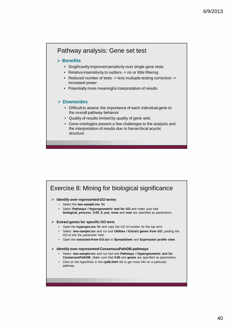
Exercise 8: Mining for biological significance

Identify over-represented GO terms• Select the two-sample.tsv file• Select Pathways / Hypergeometric test for GO and make sure that

biological_process, 0.05, 5, yes, none and over are specified as parameters.

Extract genes for specific GO term• Open the hypergeo.tsv file and copy the GO id number for the top term.• Select two-sample.tsv and run tool Utilities / Extract genes from GO, pasting the

GO id into the parameter field.• Open the extracted-from-GO.tsv in Spreadsheet and Expression profile view.

Identify over-represented ConsensusPathDB pathways • Select two-sample.tsv and run tool and Pathways / Hypergeometric test for

ConsensusPathDB. Make sure that 0.05 and genes are specified as parameters.• Click on the hyperlinks in the cpdb.html tile to get more info on a particular

pathway.

6/9/2013

41

Exercise 9: Gene set test

Identify differentially expressed KEGG pathways• Select the normalized.tsv file and Pathways / Gene set test. Make sure

that group, KEGG, yes, 4, 600 and 600 are specified as parameters.• Explore the results both in tabular fromat and graphically in the global-test-

result-table.tsv and multtest.png files, respectively.

Automatic analysis workflows

6/9/2013

42

Workflow – reusing and sharing your analysis pipeline

Chipster allows you to save your analysis workflow as a ”macro”, which can be applied to another normalized dataset

All the analysis steps and their parameters are saved as a script file to your computer

You can share the workflow file with a collaborator

In addition to user-made workflows, Chipster contains ready-made workflows for finding and analyzing differentially expressed genes, miRNAs or proteins.

Saving and using workflows

After completing your analysis, select the starting point for your workflow and click ”Workflow/ Save starting from selected”

You can save the workflow file anywhere on your computer and change its name, but the ending must be .bsh.

You can apply the workflow to another normalized dataset by selecting

• Workflow->Open and run• Workflow->Run recent (if you saved the

workflow recently).

6/9/2013

43

Changing the workflow fileYou can change parameters directly to the workflow file

Exercise 10: Saving a workflow

Save a workflow• Prune your workflow if necessary (remove cyclic structures)• Select the file normalized.tsv and click on the Workflow / Save starting

from selected. Give your workflow a meaningful name and save it.

Documents

Normalization - German Cancer Research Center · 6/9/2013 3 Normalization of Agilent data in Chipster Background correction • Background treatment None, Subtract, Edwards, Normexp