Embed Size (px)
Citation preview

Computers and Chemical Engineering 27 (2003) 1741�/1754
www.elsevier.com/locate/compchemeng
Nonlinear system identification and model reduction using artificialneural networks
Vinay Prasad *, B. Wayne Bequette
Howard P. Isermann Department of Chemical Engineering, Rensselaer Polytechnic Institute, CII 6015, 110 8th Street, Troy, NY 12180-3590, USA
Received 9 April 2002; received in revised form 29 May 2003; accepted 29 May 2003
Abstract
We present a technique for nonlinear system identification and model reduction using artificial neural networks (ANNs). The
ANN is used to model plant input�/output data, with the states of the model being represented by the outputs of an intermediate
hidden layer of the ANN. Model reduction is achieved by applying a singular value decomposition (SVD)-based technique to the
weight matrices of the ANN. The sequence of state values is used to convert the model to a form that is useful for state and
parameter estimation. Examples of chemical systems (batch and continuous reactors and distillation columns) are presented to
demonstrate the performance of the ANN-based system identification and model reduction technique.
# 2003 Elsevier Ltd. All rights reserved.
Keywords: Nonlinear system identification; Model reduction; Artificial neural networks
1. Motivation
Strategies for state, parameter and disturbance esti-
mation have been extensively researched in chemical
process control. Every estimator design requires a
nominal state-space model around which the estimator
is constructed. In many cases, a first-principles mechan-
istic model constructed from material and energy
balances is used as the nominal model. However, it
may not always be possible to construct a satisfactory
nominal model for a given process. In other cases, the
mechanistic state-space model developed may be of very
high order. In the case of distributed parameter systems,
the conversion of the original system model (described
by partial differential equations) into a system of
ordinary differential equations (ODEs) invariably leads
to a very high order model. Such models are often
unsuitable for direct application in an estimation frame-
work. Constructing appropriate augmented parameter
* Corresponding author. Present address: Controls Engineering
Group, H2Gen Innovations, Inc., 4335 Taney Avenue, 402,
Alexandria, VA 22304, USA. Tel.: �/1-703-823-3305; fax: �/1-703-
212-4898.
E-mail address: [email protected] (V. Prasad).
0098-1354/03/$ - see front matter # 2003 Elsevier Ltd. All rights reserved.
doi:10.1016/S0098-1354(03)00137-6
and disturbance structures is non-trivial for these high
order models.
This indicates the need for a method for system
identification and model reduction to create models thatare convenient for estimator and controller design. For
linear systems, subspace identification methods are used
for constructing state-space models from input�/output
data, and model reduction is achieved by using balanced
truncation. These techniques, however, are not directly
applicable to nonlinear systems. In this paper, we
explore techniques for nonlinear system identification
and model reduction based on artificial neural networks(ANNs). We propose a new method to construct
reduced order nonlinear state-space models from in-
put�/output data using ANNs. The model identified
using ANNs and input�/output data is then transformed
into a form that is well-suited for estimator and
controller design.
2. Background
An important step in the design of estimators andcontrollers for chemical processes is the development of
an accurate model of the system. This nominal model is
then used as the basis for state estimator design. First-
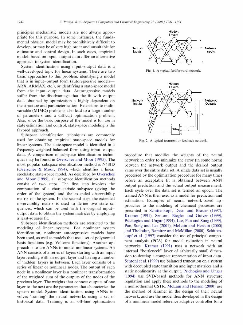
Fig. 1. A typical feedforward network.
Fig. 2. A typical recurrent or feedback network.
V. Prasad, B.W. Bequette / Computers and Chemical Engineering 27 (2003) 1741�/17541742
principles mechanistic models are not always appro-
priate for this purpose. In some instances, the funda-
mental physical model may be prohibitively difficult to
develop, or may be of very high order and unsuitable forestimator and control design. In such cases, empirical
models based on input�/output data offer an alternative
approach to system identification.
System identification using input�/output data is a
well-developed topic for linear systems. There are two
basic approaches to this problem: identifying a model
that is in input�/output form (autoregressive models*/
ARX, ARMAX, etc.), or identifying a state-space modelfrom the input�/output data. Autoregressive models
suffer from the disadvantage that the fit with output
data obtained by optimization is highly dependent on
the structure and parameterization. Extensions to multi-
variable (MIMO) problems also lead to a large number
of parameters and a difficult optimization problem.
Also, since the basic purpose of the model is for use in
state estimation and control, state-space modeling is thefavored approach.
Subspace identification techniques are commonly
used for obtaining empirical state-space models for
linear systems. The state-space model is identified in a
frequency-weighted balanced form using input�/output
data. A comparison of subspace identification techni-
ques may be found in Overschee and Moor (1995). The
most popular subspace identification method is N4SID(Overschee & Moor, 1994), which identifies a linear
stochastic state-space model. As described by Overschee
and Moor (1995), all subspace identification methods
consist of two steps. The first step involves the
computation of a characteristic subspace (giving the
order of the system) and the extended observability
matrix of the system. In the second step, the extended
observability matrix is used to define two state se-quences, which can be used with the original input�/
output data to obtain the system matrices by employing
a least-squares fit.
Subspace identification methods are restricted to the
modeling of linear systems. For nonlinear system
identification, nonlinear autoregressive models have
been used, as well as models that use a set of polynomial
basis functions (e.g. Volterra functions). Another ap-proach is to use ANNs to model nonlinear systems. An
ANN consists of a series of layers starting with an input
layer, ending with an output layer and having a number
of ‘hidden’ layers in between. Each layer consists of a
series of linear or nonlinear nodes. The output of each
node in a nonlinear layer is a nonlinear transformation
of the weighted sum of the outputs of the nodes of the
previous layer. The weights that connect outputs of onelayer to the next are the parameters that characterize the
system model. System identification using ANNs in-
volves ‘training’ the neural networks using a set of
historical data. Training is an off-line optimization
procedure that modifies the weights of the neural
network in order to minimize the error (in some norm)
between the network output and the desired output
value over the entire data set. A single data set is usually
processed by the optimization procedure for many times
before an acceptable fit is obtained between ANN
output prediction and the actual output measurement.
Each cycle over the data set is termed an epoch. The
trained ANN is then used as a model for prediction and
estimation. Examples of neural network-based ap-
proaches to the modeling of chemical processes are
presented in Schittenkopf, Deco and Brauer (1997),
Kramer (1991), Sentoni, Biegler and Guiver (1999),
Psichogios and Ungar (1994), Lee, Pan and Sung (1999),
Pan, Sung and Lee (2001), McLain and Henson (2000)
and Tholodur, Ramirez and McMillan (2000). Schitten-
kopf et al. (1997) consider the use of principal compo-
nent analysis (PCA) for model reduction in neural
networks. Kramer (1991) uses a network with an
internal ‘‘bottleneck’’ layer of arbitrarily small dimen-
sion to develop a compact representation of input data.
Sentoni et al. (1999) use balanced truncation on a system
with decoupled state transition and input matrices and a
static nonlinearity at the output. Psichogios and Ungar
(1994) use SVD-based methods for ANN structure
regulation and apply these methods to the modeling of
a nonisothermal CSTR. McLain and Henson (2000) use
the method of Kramer in the design of their neural
network, and use the model thus developed in the design
of a nonlinear model reference adaptive controller for a
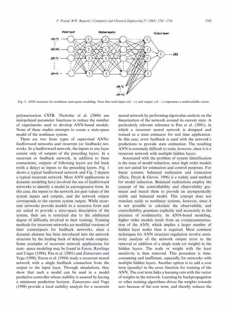
Fig. 3. ANN structure for nonlinear state-space modeling. Note that each input u (k�/i ) and output y (k�/i ) represents a multivariable vector.
V. Prasad, B.W. Bequette / Computers and Chemical Engineering 27 (2003) 1741�/1754 1743
polymerization CSTR. Tholodur et al. (2000) use
interpolated parameter functions to reduce the number
of experiments used to develop ANN-based models.
None of these studies attempts to create a state-space
model of the nonlinear system.
There are two basic types of supervised ANNs:
feedforward networks and recurrent (or feedback) net-
works. In a feedforward network, the inputs to any layer
consist only of outputs of the preceding layers. In a
recurrent or feedback network, in addition to these
connections, outputs of following layers are fed back
(with a delay) as inputs to the preceding layers. Fig. 1
shows a typical feedforward network and Fig. 2 depicts
a typical recurrent network. Most ANN applications in
dynamic modeling have involved the use of feedforward
networks to identify a model in autoregressive form. In
this case, the inputs to the network are past values of the
system inputs and outputs, and the network output
corresponds to the current system output. While recur-
rent networks provide models in a recursive form and
are suited to provide a state-space description of the
system, their use is restricted due to the additional
degree of difficulty involved in their training. Training
methods for recurrent networks are modified versions of
their counterparts for feedback networks, since a
dynamic element has been introduced into the network
structure by the feeding back of delayed node outputs.
Some examples of recurrent network applications for
state�/space modeling may be found in Eaton, Rawlings
and Ungar (1994), Pan et al. (2001) and Zamarreno and
Vega (1998). Eaton et al. (1994) study a recurrent neural
network with a single feedback connection from the
output to the input layer. Through simulations, they
show that such a model can be used in a model
predictive controller whose stability is assured by having
a minimum prediction horizon. Zamarreno and Vega
(1998) provide a local stability analysis for a recurrent
neural network by performing eigenvalue analysis on the
linearization of the network around its current state. A
particularly relevant reference is Pan et al. (2001), in
which a recurrent neural network is designed and
trained as a state estimator for real time application.
In this case, error feedback is used with the network’s
predictions to provide state estimation. The resulting
ANN is extremely difficult to train, however, since it is a
recurrent network with multiple hidden layers.
Associated with the problem of system identification
is the issue of model reduction, since high order models
are not suited for estimation and control purposes. For
linear systems, balanced realization and truncation
(Zhou, Doyle & Glover, 1996) is a widely used method
for model reduction. Balanced realizations employ the
concept of the controllability and observability gra-
mians and match them to provide an asymptotically
stable and balanced model. This concept does not
translate easily to nonlinear systems, however, since it
is not possible to calculate the observability and
controllability gramians explicitly and accurately in the
presence of nonlinearity. In ANN-based modeling,
higher order models result from an overparameteriza-
tion of the ANN, which implies a larger number of
hidden layer nodes than is required. Most common
techniques for ANN structure regulation involve sensi-
tivity analysis of the network output error to the
removal or addition of a single node (or weight) in the
hidden layers. The node or weight with the least
sensitivity is then removed. This procedure is time-
consuming and inefficient, especially for networks with
multiple hidden layers. Another option is to add a cost
term (penalty) in the error function for training of the
ANN. The cost term links a learning rate with the vector
of weights in the network. Learning by backpropagation
or other training algorithms drives the weights towards
zero because of the cost term, and thereby reduces the

Fig. 4. A representative plot of the type of inputs used for generation
of training and prediction data. The abscissa represents the index of
data points and the ordinate values of the input sequence.
V. Prasad, B.W. Bequette / Computers and Chemical Engineering 27 (2003) 1741�/17541744
number of free parameters. Deciding on the actual form
of the cost function and the learning rate is a non-trivial
task, however, and is system-dependent.
A more promising approach for ANN structureregulation and reduction of overfitting is the use of
singular value decomposition (SVD) or PCA-based
methods. SVD-based methods have been investigated
by Psichogios and Ungar (1994), Schittenkopf et al.
(1997), Emmerson and Dampier (1993) and Hu, Xue
and Tompkins (1991). All of these studies involve using
SVD as an explicit model selection method to remove
redundant hidden nodes during network training. TheSVD is applied on linear layers, or on nonlinear layers
before the nonlinear transformation is applied. Correla-
tions between the outputs of nodes lead to small singular
values corresponding to those outputs. The nodes
corresponding to the small singular values are redun-
dant and are removed from the network, thus reducing
the degree of overparameterization. Two different
approaches to model reduction are presented in Sentoniet al. (1999) and Kramer (1991). Sentoni et al. use
balanced truncation on a neural network system con-
sisting of a linear input-state relationship. Their for-
mulation is only applicable to systems with static
nonlinearities. Kramer’s technique is concerned solely
with nonlinear PCA, and assumes that full state
information is available, i.e. all states are measured
outputs. A network containing an internal ‘‘bottleneck’’layer of small size is constructed that maps the state
information back onto itself. The outputs of the nodes
of the bottleneck layer represent the reduced
state vector. The choice of the size of the
bottleneck layer is arbitrary, with the only
guideline for model reduction being that the number
of bottleneck nodes is smaller than the number of
original states.
3. System identification and model reduction using
artificial neural networks
A new formulation for system identification using
neural networks is presented in this section. The basic
principle is to train a neural network based on input�/
output data, and to use the dynamic information storedin the outputs of an intermediate hidden layer to
represent the state vector of the model. SVD is then
performed on each of the layers in the network to
remove redundant nodes and thus provide a compact
model. The difference from earlier formulations is in the
use of SVD as an explicit criterion for model reduction
and node truncation, and in the fact that the network
trained on the basis of plant output data is used toprovide an empirical state-space model of the system.
Previous approaches based on developing nonlinear
state-space models from input�/output data using neural
networks have not addressed the issue of overparame-
terization resulting from using an arbitrary number of
nodes in the hidden layers of the ANN. Another feature
of the proposed approach is the use of the state
information from the ANN model to construct a
reduced order model by constructing a state transforma-
tion matrix. This requires information about the states
of the original higher order model.
The state space modeling may, in principle, be
performed using recurrent or feedforward networks. In
the description that follows, the method is described for
the case of a feedforward network. In this situation, the
inputs to the ANN are past plant input and output
values, and the outputs of the ANN are current and
future plant outputs. Future plant outputs are consid-
ered because models used in predictive control need to
be accurate multi-step predictors and not just provide
good one-step ahead prediction. The past window of
system inputs and outputs chosen as ANN inputs must
be of sufficient length in time to capture the essentials of
the plant dynamics.
Fig. 3 presents the framework of the proposed ANN
for nonlinear system identification. The network is

Table 1
Parameter values for bioreactor
mmax 0.55 h�1
KCG 1.20 g l�1
Y 0.45 g g�1
sI �/0.02
p1 2.8 l g�1
p2 4.0 l g�1
rI ,max 1.0 h�1
KCI 9.0 g l�1
rP ,max 1.0 h�1
KCP 6.2 g l�1
fI 0 0.0008 g l�1
KI 0.03 g l�1
Fig. 5. ANN training performance for induced bacterial protein
bioreactor. Output y1 represents the cell mass and y2 represents the
protein concentration. The abscissa is the index of data points, and the
sample time is 0.1 h.
Fig. 6. ANN prediction performance for induced bacterial protein
bioreactor. Output y1 represents the cell mass and y2 represents the
protein concentration. The dotted line represents the ANN predictions
and the solid line the true plant output. The abscissa is the index of
data points, and the sample time is 0.1 h.
V. Prasad, B.W. Bequette / Computers and Chemical Engineering 27 (2003) 1741�/1754 1745
composed of two parts, one which maps the input-state
relation (xk�1�/f(xk , uk)) and another which maps the
state-output relation (yk �/g (xk , uk)). Note that non-
linear nodes in Fig. 3 are represented with an enclosed
sigmoid, while linear nodes are left blank. The network
has four hidden layers, with three of them using non-
linear nodes. The output layer is nonlinear. The states
are represented by the outputs of the linear hidden layer,
and are thus a linear combination of the outputs of the
second hidden layer. From the network structure, it is
seen that two nonlinear layers are used in the mapping
of each function, the input-state relation and the state-
output relation. It is known that a network with twononlinear layers is capable of approximating a nonlinear
function of arbitrary order (Weigend, Huberman &
Rumelhart, 1990), which is what motivates the choice of
the network structure. The outputs of the ANN can
include future plant outputs (up to yk�p) and the ANN
can be trained as a multi-step predictor. However, this
will require the inclusion of future plant inputs as ANN
inputs in the hidden layer (along with the states), as wellas keeping a separate state-output network for each
future output (to maintain the condition of causality). In
the examples in this paper, we restrict ourselves to a one-
step ahead predictor, meaning that a single ANN maps
the state-output relation.
The procedure for removal of overfitting in the ANN
model is described below. Consider a layer with non-
linear nodes, where the output of the i th node is givenby:
zi �s
�Xj
Wij � uj�W biasi
�(1)
where W is the matrix of weights that links the previous
layer to the current layer and u is the vector of inputs to
the current layer (outputs of the previous layer). s is the

Fig. 7. ANN prediction performance with reduced order modeling for
induced bacterial protein bioreactor. Output y1 represents the cell mass
and y2 represents the protein concentration. The abscissa is the index
of data points, and the sample time is 0.1 h.
Fig. 8. Prediction performance of transformed reduced state model for
induced bacterial protein bioreactor. Output y1 represents the cell mass
and y2 represents the protein concentration. The abscissa is the time in
hours.
V. Prasad, B.W. Bequette / Computers and Chemical Engineering 27 (2003) 1741�/17541746
nonlinear transformation, which is taken to be the
hyperbolic tangent function in this case. Wbias representsthe weight associated with the bias input to each node.
The output of the node before the nonlinear transfor-
mation is applied is given by:
zlini �
Xj
Wij � uj�W biasi (2)
Overfitting in terms of the presence of redundant
nodes in a layer may be diagnosed by searching for
correlations between the outputs of the nodes. SVD is a
method for detecting linear correlations and hence an
overdetermined problem. SVD is applied to the outputs
of each layer (before the nonlinear transformation is
applied). This is justified in the sense of removing linearcorrelations in the input data that is presented to each
nonlinear node. The procedure is illustrated for an
arbitrary choice of two consecutive layers in the net-
work, which are referred to as layer 1 and layer 2 for
convenience. The output of layer 1 acts as an input to
the nodes of layer 2. Consider the relation:
SW �Zlin (3)
where S is a matrix containing as columns the outputs
of the nodes of layer 1 for each input data sample, i.e. S
contains values of u for each data sample as its columns.
W is the weight matrix connecting the layers and the
matrix Zlin is the set of outputs of the nodes of layer 2
over all data samples. SVD is then performed on thematrix S to decompose it into the form:
S�USVT (4)
S is a diagonal matrix containing the singular values
of S on its diagonal. SVD may be used as a least squarestool for removal of redundant nodes by removing nodes
that correspond to small or zero singular values. This
implies reducing the size of S, and corresponding
reduction in the size of U and V by removal of columns
and rows to create a lower dimensional matrix S . Since
the dimension of S reflects the number of nodes in layer
1, this reduces the number of nodes in layer 1 and acts as
a mechanism for model reduction. The number ofweight connections in W is reduced correspondingly.
This procedure is applied for all possible layers in the
ANN to reduce overfitting in all the layers. The network
is retrained after the SVD procedure has been applied.
This procedure is carried out in a couple of iterations,
where the ANN is trained and then pruned, and the
process is repeated until further pruning and training do
not significantly change the weights of the network. In astrict sense, SVD should be applied only to spatially
correlated data, which have no temporal correlation.
The data used in our procedure contains temporal

Table 2
Parameter values for distillation column
Hc 30 mol
Hr 30 mol
Ht 20 mol
a 5
Lf 10.0 mol (min)�1
xf 0.5
L 27.3755 mol (min)�1
V 32.3755 mol (min)�1
Fig. 9. ANN training performance for distillation column. Output y1
represents the liquid composition in the reboiler (x1) and y2 represents
x4, the liquid composition in tray 4. The solid line represents the true
plant output and the dotted line the ANN prediction. The abscissa is
the index of data points, and the sample time is 0.1 min.
Fig. 10. ANN prediction performance for distillation column. Output
y1 represents the liquid composition in the reboiler (x1) and y2
represents x4, the liquid composition in tray 4. The abscissa is the
index of data points, and the sample time is 0.1 min.
V. Prasad, B.W. Bequette / Computers and Chemical Engineering 27 (2003) 1741�/1754 1747
correlations, since they describe the dynamic behavior of
a system. However, since the SVD procedure is applied
to the entire data set, which includes the entire range of
behavior of the system, it is justified in a practical sense
to use SVD as a model reduction method. This is borne
out in the results described in the next section.
For the case of model reduction, we consider the layer
defining the states of the ANN model. Referring again
to Fig. 3, since the states represented by the output of
the intermediate linear layer are just a linear combina-
tion of the dynamic responses of the previous nonlinear
layer, the outputs of the second nonlinear layer may be
used equally well to describe the states of the system.
SVD applied on the relation between the second and
third hidden layers of the ANN then removes redundant
nodes from the second nonlinear layer and hence
reduces the number of states in the ANN model. Note
that SVD is applied to the relation between the input
layer and the first hidden layer, which ensures that input
noise and redundancy in input data is filtered out.We make a distinction between the proposed method
and two similar approaches. Kramer (1991) uses a three-
hidden layer network to map the system states on to
themselves, with the intermediate hidden layer contain-
ing an arbitrary (small) number of nodes and represent-
ing the reduced order state space. The number of
reduced order states chosen in this case is arbitrary,
and the method applies only when full state information
is available for the original system. Lee et al. (1999) also
use a similar network with three hidden layers to obtain
state information from input�/output data. No attempt
is made to select the optimum network structure in
terms of the number of hidden layer nodes.
For the case where a high-order state space model is
available for a system and needs to be reduced to a lower
order model, an additional procedure is proposed for
construction of a model that is better suited for
estimator design and control. The proposed procedure

Fig. 11. ANN prediction performance with reduced order modeling
for distillation column. Output y1 represents the liquid composition in
the reboiler (x1) and y2 represents x4, the liquid composition in tray 4.
The abscissa is the index of data points, and the sample time is 0.1 min.
Fig. 12. Prediction performance of transformed reduced state model
for distillation column. Output y1 represents the liquid composition in
the reboiler (x1) and y2 represents x4, the liquid composition in tray 4.
The abscissa is the time in minutes.
V. Prasad, B.W. Bequette / Computers and Chemical Engineering 27 (2003) 1741�/17541748
is a modification of the approach of Lee, Eom, Chung,
Choi and Yang (2000), and involves the creation of a
state transformation matrix that projects the states ofthe original higher-order model to a lower dimensional
space. Using a state transformation matrix is better
suited in terms of retaining and translating information
on model uncertainty and possible disturbance effects
from the original model to the lower order model. The
basic principle involves using a system identification
method to create a reduced order state sequence from
input�/output data generated by the higher order model.The higher order model also generates a state sequence
of its own. Let
XN � [x(1); x(2); . . . ; x(N)]
X N � [x(1); x(2); . . . ; x(N)] (5)
where XN represents the state sequence for the original
higher order model and X N the lower order state
sequence. Lee et al. (2000) suggest the use of linear
subspace identification methods along with a balanced
truncation procedure to create the reduced order state
sequence. We use the ANN based nonlinear modelingand reduction algorithm described earlier in this section
to create the reduced order state sequence. It is known
that linear subspace methods of identification are not
very accurate in the presence of significant nonlinearity,
so a nonlinear identification procedure will providebetter results. Once the state sequences have been
generated, a transformation matrix V is generated using:
V �XNX $N (6)
where X $N denotes the Moore�/Penrose pseudo-inverse
of X N : Once the transformation matrix is constructed,
the original discrete-time nonlinear system:
x(t�1)�f (x(t); u(t))
y(t)�h(x(t); u(t)) (7)
is transformed to:
z(t�1)�V $f (Vz(t); u(t))
y(t)�h(Vz(t); u(t)) (8)
Here, V$ refers to the Moore�/Penrose inverse of V ,and the residual of the reduced state model is orthogo-
nal to the span of V .
4. Results
In this section, simulation results on a number of
nonlinear systems are presented using the techniques
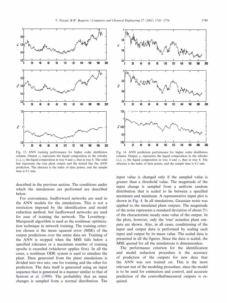
Fig. 13. ANN training performance for higher order distillation
column. Output y1 represents the liquid composition in the reboiler
(x1), y2 the liquid composition in tray 4 and y3 that in tray 6. The solid
line represents the true plant output and the dotted line the ANN
prediction. The abscissa is the index of data points, and the sample
time is 0.1 min.
Fig. 14. ANN prediction performance for higher order distillation
column. Output y1 represents the liquid composition in the reboiler
(x1), y2 the liquid composition in tray 4 and y3 that in tray 6. The
abscissa is the index of data points, and the sample time is 0.1 min.
V. Prasad, B.W. Bequette / Computers and Chemical Engineering 27 (2003) 1741�/1754 1749
described in the previous section. The conditions under
which the simulations are performed are described
below.
For convenience, feedforward networks are used in
the ANN models for the simulations. This is not a
restriction imposed by the identification and model
reduction method, but feedforward networks are used
for ease of training the network. The Levenberg�/
Marquardt algorithm is used as the nonlinear optimiza-
tion technique in network training. The training criter-
ion chosen is the mean squared error (MSE) of the
output predictions over the entire data set. Training of
the ANN is stopped when the MSE falls below a
specified tolerance or a maximum number of training
epochs is exceeded (whichever applies first). In all the
cases, a nonlinear ODE system is used to simulate the
plant. Data generated from the plant simulations is
divided into two sets, one for training and the other for
prediction. The data itself is generated using an input
sequence that is generated in a manner similar to that of
Sentoni et al. (1999). The probability that an input
changes is sampled from a normal distribution. The
input value is changed only if the sampled value is
greater than a threshold value. The magnitude of the
input change is sampled from a uniform random
distribution that is scaled to lie between a specified
maximum and minimum. A representative input plot is
shown in Fig. 4. In all simulations, Gaussian noise was
applied to the simulated plant outputs. The magnitude
of the noise represents a standard deviation of about 2%
of the characteristic steady state value of the output. In
the plots, however, only the ‘true’ noiseless plant out-
puts are shown. Also, in all cases, conditioning of the
input and output data is performed by scaling each
input and output by its mean value. The scaled data is
presented in all the figures. Since the data is scaled, the
MSE quoted for all the simulations is dimensionless.
The performance criterion for the identification
and model reduction procedure is the accuracy
of prediction of the outputs for new data that
the ANN was not trained on. This is the most
relevant test of the modeling procedure, since the model
is to be used for estimation and control, and accurate
prediction of the controlled/measured outputs is re-
quired.

V. Prasad, B.W. Bequette / Computers and Chemical Engineering 27 (2003) 1741�/17541750
5. Batch bioreactor
The first set of simulations involves the modeling of a
nonlinear batch bioreactor system presented in Tholo-dur et al. (2000). The model equations are given below
and describe foreign protein production in an inducible
bacterial system.
X �mX (9)
G��mX
Y(10)
I ��rI X (11)
P�rPX (12)
Here, X , G , I and P are the cell mass, glucose,
inducer and protein concentrations, respectively. The
system parameters are given by:
m�mmaxG
KCG � G
�sI � p1I
sI � p2I
�(13)
rI �rI ;maxI
KCI � I(14)
rP��
rP;maxG
KCP � G
��fI0 � I
KI � I
�(15)
The parameter values used are the same as those in
Tholodur et al. and are given in Table 1. In these
simulations, input excitation is not an issue due to thebatchwise nature of the process. Training data is
generated by using data from the start and end of the
batch run, and prediction is attempted using the data in
the intermediate period for testing. The sample time for
the system is 0.1 h. Fig. 5 shows the training perfor-
mance using a neural network that has the cell mass and
protein concentration as outputs. Only one-step ahead
prediction is shown, and inputs and states over two pastsampling instants were used to construct the inputs to
the ANN. The network was trained in 15 epochs using
an error stopping criterion of 10�8. The number of
nodes in each layer of the ANN is given by [4 8 8 8 8 2],
with the hidden layers each having eight nodes, and the
dimension of the inputs and outputs being 4 and 2,
respectively. Using the model structure of Fig. 3, this
implies an eight state system model. Note that the step-like change in the outputs is not a real system response,
it is indicative of the change in the nature of the data set
from the start to the end of the run. Fig. 6 shows the
prediction performance of the network. It is seen that
the ANN predictions diverge significantly from the
actual outputs for a large portion of the prediction
data. Model reduction using SVD on the ANN is now
performed. The reduced order model had the followingnumbers of nodes in its layers [4 4 3 3 4 2], which implies
a three state model. Fig. 7 shows the prediction
performance of the reduced order model. An excellent
fit to the output data is achieved. This indicates that the
system may be accurately modeled using a three-state
nonlinear ANN model. As a final exercise, the state
sequence generated by the reduced order ANN for thetraining data is used along with the corresponding state
sequence for the original system model to generate the
transformation matrix V . The transformed system is
simulated and compared against the original system,
and the results are shown in Fig. 8. The original and
reduced system outputs match almost perfectly, and so
the transformed three state system may be used as a
basis for estimator and controller design instead of theoriginal higher order system.
6. Distillation column
The second set of simulations involves a distillation
column described by Rasmussen and Jorgensen (1999).The tower consists of five trays including a total
condenser and reboiler. The system equations are given
by:
Hr
dx1
dt�(L�Lf )(x2�x1)�V (x1�y1) (16)
Ht
dx2
dt�(L�Lf )(x3�x2)�V (y1�y2) (17)
Ht
dx3
dt�Lf xf �Lx4�(L�Lf )x3�V (y2�y3) (18)
Ht
dx4
dt�L(x5�x4)�V (y3�y4) (19)
Hc
dx5
dt�V (y4�x5) (20)
yi �axi
1 � (a� 1)xi
(21)
The measured outputs are the liquid composition in
the reboiler (x1) and that in tray 4 (x4). The parameter
values are given in Table 2. The network once again uses
the inputs and outputs at the past two sampling instants
as inputs, and the next-step output as its output. This
means that there are four input and two output nodes.
Each of the hidden layers has ten nodes to begin with.The training performance of this ANN is shown in Fig.
9. The network was trained over 200 epochs using 200
data points resulting in a MSE of 0.006. The sample
time used in the generation of the data points was 0.1
min. The prediction performance of the ANN for a
different set of 200 data points is shown in Fig. 10. The
MSE over all outputs for the prediction data is 0.0445.
Fig. 11 shows the prediction performance of a reducedorder ANN obtained by performing SVD on the layers
of the original ANN and then retraining the network. It
is seen that the reduced order model provides much
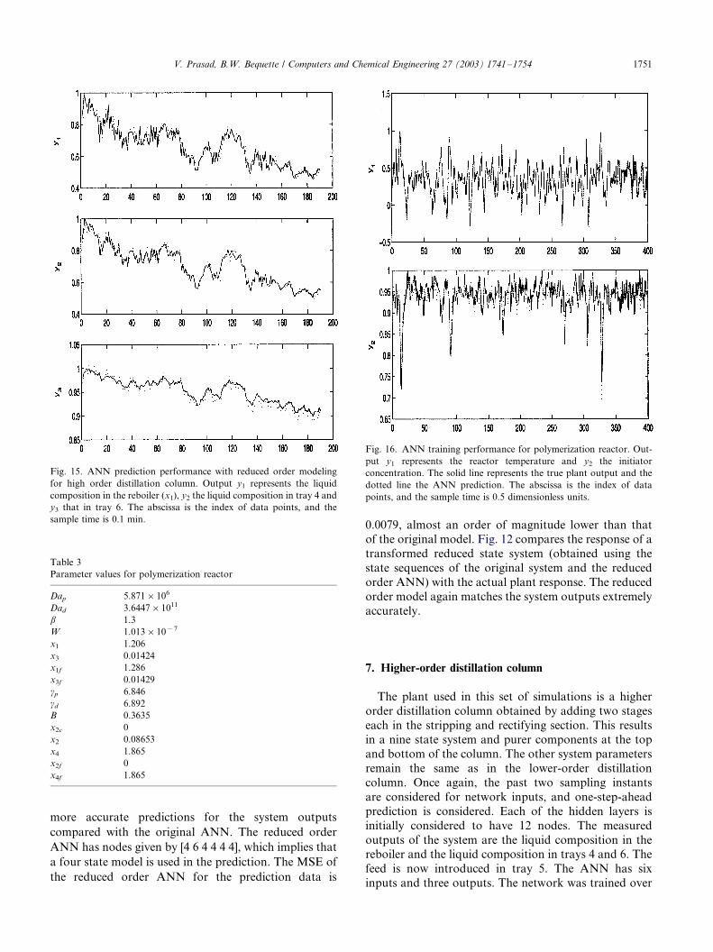
Fig. 15. ANN prediction performance with reduced order modeling
for high order distillation column. Output y1 represents the liquid
composition in the reboiler (x1), y2 the liquid composition in tray 4 and
y3 that in tray 6. The abscissa is the index of data points, and the
sample time is 0.1 min.
Table 3
Parameter values for polymerization reactor
Dap 5.871�/106
Dad 3.6447�/1011
b 1.3
W 1.013�/10�7
x1 1.206
x3 0.01424
x1f 1.286
x3f 0.01429
gp 6.846
gd 6.892
B 0.3635
x2c 0
x2 0.08653
x4 1.865
x2f 0
x4f 1.865
Fig. 16. ANN training performance for polymerization reactor. Out-
put y1 represents the reactor temperature and y2 the initiator
concentration. The solid line represents the true plant output and the
dotted line the ANN prediction. The abscissa is the index of data
points, and the sample time is 0.5 dimensionless units.
V. Prasad, B.W. Bequette / Computers and Chemical Engineering 27 (2003) 1741�/1754 1751
more accurate predictions for the system outputs
compared with the original ANN. The reduced order
ANN has nodes given by [4 6 4 4 4 4], which implies that
a four state model is used in the prediction. The MSE of
the reduced order ANN for the prediction data is
0.0079, almost an order of magnitude lower than thatof the original model. Fig. 12 compares the response of a
transformed reduced state system (obtained using the
state sequences of the original system and the reduced
order ANN) with the actual plant response. The reduced
order model again matches the system outputs extremely
accurately.
7. Higher-order distillation column
The plant used in this set of simulations is a higher
order distillation column obtained by adding two stages
each in the stripping and rectifying section. This resultsin a nine state system and purer components at the top
and bottom of the column. The other system parameters
remain the same as in the lower-order distillation
column. Once again, the past two sampling instants
are considered for network inputs, and one-step-ahead
prediction is considered. Each of the hidden layers is
initially considered to have 12 nodes. The measured
outputs of the system are the liquid composition in thereboiler and the liquid composition in trays 4 and 6. The
feed is now introduced in tray 5. The ANN has six
inputs and three outputs. The network was trained over

Fig. 17. ANN prediction performance for polymerization reactor.
Output y1 represents the reactor temperature and y2 the initiator
concentration. The abscissa is the index of data points, and the sample
time is 0.5 dimensionless units.
Fig. 18. ANN prediction performance with reduced order modeling
for polymerization reactor. Output y1 represents the reactor tempera-
ture and y2 the initiator concentration. The abscissa is the index of
data points, and the sample time is 0.5 dimensionless units.
V. Prasad, B.W. Bequette / Computers and Chemical Engineering 27 (2003) 1741�/17541752
200 epochs over a data set of 200 samples, with aprediction data set of similar size also being created. The
sampling time is kept the same as for the lower-order
column. Fig. 13 shows the trained outputs of the ANN.
The MSE on the training data is 0.5266. The prediction
performance is shown in Fig. 14. In this case, the
original ANN provides reasonably accurate predictions,
with the MSE for prediction data being 0.8643. Upon
model reduction using SVD, the number of nodes ineach layer is given by [5 5 4 4 3 3], meaning that one of
the input directions was correlated with the others and
thus was redundant. Also, a four state model is
sufficient for output prediction for the full nine state
system. The prediction performance of the reduced state
model is shown in Fig. 15. The MSE in this case is
0.7933, again proving to be more accurate than the
original overdetermined ANN model.
8. Polymerization reactor
The final set of simulations involves a CSTR used for
the free-radical polymerization of methyl methacrylate.The system equations are given below, and the para-
meter values given in Table 3 are the same as those used
by McLain and Henson (2000).
dx1
dt�x1f �x1�DapW (x)x1Ex(x2) (22)
dx2
dt�x2f �x2�BDapgpW (x)x1Ex(x2)�b(x2c�x2)
(23)
dx3
dt�x3f �x3�Dadx3Exd (x2) (24)
dx1
dt�x4f �x4 (25)
Ex(x2)�exp
�x2
1 �x2
gp
�(26)
Exd(x2)�exp
�gdx2
1 �x2
gp
�(27)
x1 represents the monomer concentration, x2 the
reactor temperature, x3 the initiator concentration and
x4 the solvent concentration, all in dimensionless vari-
ables. x2 and x3 are the measured system outputs. Onceagain, system inputs and outputs at the past two
sampled instants are used to construct inputs and
outputs to the ANN. This means that there are four

Table 4
System identification results
System System states ANN states Training MSE Prediction MSE Reduced states Prediction MSE
Batch bioreactor 4 8 1.0e�/8 0.1504 3 0.0130
Distillation column 5 9 0.006 0.0445 4 0.0079
Distillation column 9 12 0.5266 0.8643 4 0.7933
Polymerization reactor 4 8 0.0050 0.3415 3 0.0200
V. Prasad, B.W. Bequette / Computers and Chemical Engineering 27 (2003) 1741�/1754 1753
input nodes and two output nodes. The first hiddenlayer has 15 nodes, and all the others have eight nodes,
respectively. 400 data points are used in the training
data set, and a similar number are used in the prediction
data set. The sampling time is chosen to be 0.5
dimensionless units. The network was trained over 200
epochs. Fig. 16 shows the training performance of the
ANN. The MSE for the training data is 0.0050. Fig. 17
shows the prediction performance of the ANN. It can beseen that the ANN predictions are not very accurate,
with the MSE of the prediction being 0.3415. Upon
application of SVD, the reduced order ANN contains
hidden layers with 14, 3, 5 and 4 nodes, respectively,
implying a three state reduced order model. The
prediction performance of the reduced order model is
presented in Fig. 18. The predictions are much more
accurate, especially for the reactor temperature. Under-predictions of the deviations in the initiator concentra-
tion are observed. The MSE for the predictions in this
case is 0.0220, which is again a sizable improvement
over the original ANN model, even though greater
accuracy is desirable, perhaps by further training of the
network.
A summary of the results for the examples presented
above is given in Table 4. In all cases, the predictionMSE for the reduced order model is smaller than the
prediction MSE for the original ANN model, demon-
strating the efficacy of the model reduction techniques.
9. Summary
A technique for nonlinear system identification and
model reduction using ANNs has been proposed anddemonstrated in this paper. The method uses an ANN
to model input�/output data, with the system states
being given by the outputs of a hidden layer. Model
reduction is achieved by reducing overparameterization
of the ANN by removing redundant nodes using a SVD
based technique. In all the examples considered, the
reduced model ANN provides equivalent or improved
output prediction over the original overparameterizednetwork. Significant reduction in the number of states in
the model is also achieved. The state sequence of the
ANN model is used to construct a state transformation
matrix which maps the original higher order system into
a lower order state space and is a useful tool for model
reduction. Extension of the method for use in recurrent
networks is relatively simple, and is desirable because
nonlinear discrete state-space models are represented
compactly in such a form. This comes at the expense of
posing a more difficult optimization problem in the
training of the ANN.
References
Eaton, J. W., Rawlings, J. B., & Ungar, L. H. (1994). Stability of
neural net based model predictive control. In Proceedings of the
American control conference (pp. 2481�/2485).
Emmerson, M. D., & Dampier, R. I. (1993). Determining and
improving the fault tolerance of multilayer perceptrons in a
pattern�/recognition application. IEEE Transactions on Neural
Network 4 , 788�/793.
Hu, Y. H., Xue, Q., & Tompkins, W. J. (1991). Structural simplifica-
tion of a feed-forward, multi-layer perceptron artificial neural
network. In Proceedings of the international conference on acoustics,
speech and signal processing (pp. 1061�/1064).
Kramer, M. A. (1991). Nonlinear principal component analysis using
autoassociative neural networks. American Institute of Chemical
Engineering Journal 37 , 233�/243.
Lee, K. S., Eom, Y., Chung, J. W., Choi, J., & Yang, D. (2000). A
control-relevant model reduction technique for nonlinear systems.
Computers and Chemical Engineering 24 , 309�/315.
Lee, J. H., Pan, Y., & Sung, S. W. (1999). A numerical projection-
based approach to nonlinear model reduction and identification. In
Proceedings of the American control conference (pp. 1568�/1572).
McLain, R. B., & Henson, M. A. (2000). Principal component analysis
for nonlinear model reference adaptive control. Computers and
Chemical Engineering 24 , 99�/110.
Overschee, P. V., & Moor, B. D. (1994). N4SID: subspace algorithms
for the identification of combined deterministic�/stochastic systems.
Automatica 30 , 75�/93.
Overschee, P. V., & Moor, B. D. (1995). A unifying theorem for three
subspace system identification algorithms. Automatica 31 , 1853�/
1864.
Pan, Y., Sung, S. W., & Lee, J. H. (2001). Data-based construction of
feedback-corrected nonlinear prediction model using feedback
neural networks. Control Engineering Practice 9 , 859�/867.
Psichogios, D. C., & Ungar, L. H. (1994). SVD-NET: an algorithm
that automatically selects network structure. IEEE Transactions on
Neural Networks 5 , 513�/515.
Rasmussen, K. H., & Jorgensen, S. B. (1999). Parametric uncertainty
modeling for robust control: a link to identification. Computers and
Chemical Engineering 23 , 987�/1003.

V. Prasad, B.W. Bequette / Computers and Chemical Engineering 27 (2003) 1741�/17541754
Schittenkopf, C., Deco, G., & Brauer, W. (1997). Two strategies to
avoid overfitting in feedforward networks. Neural Networks 10 ,
505�/516.
Sentoni, G. B., Biegler, L. T., & Guiver, J. P. (1999). Model reduction
for nonlinear DABNet models. In Proceedings of the American
control conference (pp. 2052�/2056).
Tholodur, A., Ramirez, W. F., & McMillan, J. D. (2000). Interpolated
parameter functions for neural network models. Computers and
Chemical Engineering 24 , 2545�/2553.
Weigend, A. S., Huberman, B. A., & Rumelhart, D. E. (1990).
Predicting the future: a connectionist approach. International
Journal of Neural Systems 1 , 193�/209.
Zamarreno, J. M., & Vega, P. (1998). State space neural
network. Properties and application. Neural Networks 11 , 1099�/
1112.
Zhou, K., Doyle, J. C., & Glover, K. (1996).
Robust and optimal control . Englewood Cliffs, NJ: Prentice
Hall.