Nonlinear Structural Materials Module - lost … · he Nonlinear Structural Materials Module contains materials which are used in combination with the Solid Mechanics ... † Large

VERSION 4.4

User s Guide

Nonlinear Structural Materials Module

C o n t a c t I n f o r m a t i o n

Visit the Contact COMSOL page at www.comsol.com/contact to submit general inquiries, contact Technical Support, or search for an address and phone number. You can also visit the Worldwide Sales Offices page at www.comsol.com/contact/offices for address and contact information.

If you need to contact Support, an online request form is located at the COMSOL Access page at www.comsol.com/support/case.

Other useful links include:

• Support Center: www.comsol.com/support

• Product Download: www.comsol.com/support/download

• Product Updates: www.comsol.com/support/updates

• COMSOL Community: www.comsol.com/community

• Events: www.comsol.com/events

• COMSOL Video Center: www.comsol.com/video

• Support Knowledge Base: www.comsol.com/support/knowledgebase

Part number: CM022901

N o n l i n e a r S t r u c t u r a l M a t e r i a l s M o d u l e U s e r ’ s G u i d e © 1998–2013 COMSOL

Protected by U.S. Patents 7,519,518; 7,596,474; 7,623,991; and 8,457,932. Patents pending.

This Documentation and the Programs described herein are furnished under the COMSOL Software License Agreement (www.comsol.com/sla) and may be used or copied only under the terms of the license agreement.

COMSOL, COMSOL Multiphysics, Capture the Concept, COMSOL Desktop, and LiveLink are either registered trademarks or trademarks of COMSOL AB. All other trademarks are the property of their respective owners, and COMSOL AB and its subsidiaries and products are not affiliated with, endorsed by, sponsored by, or supported by those trademark owners. For a list of such trademark owners, see www.comsol.com/tm.

Version: November 2013 COMSOL 4.4

http://www.comsol.com/sla/

http://www.comsol.com/tm/

http://www.comsol.com/contact/

http://www.comsol.com/contact/offices/

http://www.comsol.com/support/case/

http://www.comsol.com/support/

http://www.comsol.com/support/download/

http://www.comsol.com/support/updates/

http://www.comsol.com/community/

http://www.comsol.com/events/

http://www.comsol.com/video/

http://www.comsol.com/support/knowledgebase/

C o n t e n t s

C h a p t e r 1 : I n t r o d u c t i o n

About the Nonlinear Structural Materials Module 6

What Can the Nonlinear Structural Materials Module Do? . . . . . . . 6

Where Do I Access the Documentation and Model Libraries?. . . . . . 7

Overview of the User’s Guide 10

C h a p t e r 2 : N o n l i n e a r S t r u c t u r a l M a t e r i a l s T h e o r y

Hyperelastic Material Theory 12

Working with Hyperelastic Materials . . . . . . . . . . . . . . . 12

Lagrangian Formulation . . . . . . . . . . . . . . . . . . . . 13

Modeling Large Deformations . . . . . . . . . . . . . . . . . . 14

Modeling Elastic Deformations. . . . . . . . . . . . . . . . . . 16

Thermal Expansion . . . . . . . . . . . . . . . . . . . . . . 17

Large Strain Plasticity Theory . . . . . . . . . . . . . . . . . . 18

Isochoric Elastic Deformation . . . . . . . . . . . . . . . . . . 18

Nearly Incompressible Hyperelastic Materials . . . . . . . . . . . . 20

Theory for the Predefined Hyperelastic Material Models . . . . . . . . 22

Elastoplastic Material Theory 32

Introduction to Small and Large Plastic Strains. . . . . . . . . . . . 32

Plastic Flow for Small Strains . . . . . . . . . . . . . . . . . . 34

Isotropic Plasticity . . . . . . . . . . . . . . . . . . . . . . 35

Yield Function . . . . . . . . . . . . . . . . . . . . . . . . 37

Hill Orthotropic Plasticity . . . . . . . . . . . . . . . . . . . 37

C O N T E N T S | 3

4 | C O N T E N T S

Hardening Models . . . . . . . . . . . . . . . . . . . . . . 40

Plastic Flow for Large Strains . . . . . . . . . . . . . . . . . . 43

Numerical Solution of the Elastoplastic Conditions . . . . . . . . . . 45

References for Elastoplastic Materials . . . . . . . . . . . . . . . 45

Creep and Viscoplasticity Theory 47

About Creep . . . . . . . . . . . . . . . . . . . . . . . . 47

Fundamental Creep Material Models . . . . . . . . . . . . . . . 49

Solver Settings for Creep and Viscoplasticity . . . . . . . . . . . . 53

Creep Material Models for Metals and Crystalline Solids . . . . . . . . 53

Viscoplasticity . . . . . . . . . . . . . . . . . . . . . . . . 57

References for Nonlinear Structural Materials 59

C h a p t e r 3 : N o n l i n e a r S t r u c t u r a l M a t e r i a l s

Working with Nonlinear Structural Materials 62

Adding a Material to a Solid Mechanics Interface . . . . . . . . . . . 62

Hyperelastic Material . . . . . . . . . . . . . . . . . . . . . 63

Linear Elastic Material . . . . . . . . . . . . . . . . . . . . . 67

Creep . . . . . . . . . . . . . . . . . . . . . . . . . . . 67

Viscoplasticity . . . . . . . . . . . . . . . . . . . . . . . . 70

Plasticity . . . . . . . . . . . . . . . . . . . . . . . . . . 71

1

I n t r o d u c t i o n

This guide describes the Nonlinear Structural Materials Module, an optional add-on package for COMSOL Multiphysics® designed to assist you to model structural behavior that includes nonlinear materials. The module is an add-on to the Structural Mechanics Module or the MEMS Module and extends it with support for modeling nonlinear materials, including hyperelasticity, creep, plasticity, and viscoplasticity.

This chapter introduces you to the capabilities of this module. A summary of the physics interfaces and where you can find documentation and model examples is also included. The last section is a brief overview with links to each chapter in this guide.

In this chapter:

• About the Nonlinear Structural Materials Module

• Overview of the User’s Guide

5

6 | C H A P T E R

Abou t t h e Non l i n e a r S t r u c t u r a l Ma t e r i a l s Modu l e

These topics are included in this section:

• What Can the Nonlinear Structural Materials Module Do?

• Where Do I Access the Documentation and Model Libraries?

What Can the Nonlinear Structural Materials Module Do?

The Nonlinear Structural Materials Module is an optional package that extends the Structural Mechanics Module to studies that include structural mechanics with nonlinear material behavior. It is designed for researchers, engineers, developers, teachers, and students that want to simulate nonlinear structural materials, including a full range of possible multiphysics couplings.

The module provides an extensive set of nonlinear structural material models, including the following materials:

• Predefined and user-defined hyperelastic materials: neo-Hookean, Mooney-Rivlin, Saint-Venant Kirchhoff, Arruda-Boyce, Ogden, and others.

• Small-strain and large-strain plasticity models using different hardening models.

• User-defined plasticity, flow rule and hardening models.

• Predefined and user-defined creep and viscoplastic material models: Norton, Garofalo, Anand, potential, volumetric, deviatoric, and others.

N O T E A B O U T M A T E R I A L S

The Physics Interfaces and Building a COMSOL Model in the COMSOL Multiphysics Reference Manual

The material property groups (including all associated properties) can be added to models from the Material page. See Materials in the COMSOL Multiphysics Reference Manual.

1 : I N T R O D U C T I O N

Where Do I Access the Documentation and Model Libraries?

A number of Internet resources provide more information about COMSOL, including licensing and technical information. The electronic documentation, topic-based (or context-based) help, and the Model Libraries are all accessed through the COMSOL Desktop.

T H E D O C U M E N T A T I O N A N D O N L I N E H E L P

The COMSOL Multiphysics Reference Manual describes all core physics interfaces and functionality included with the COMSOL Multiphysics license. This book also has instructions about how to use COMSOL and how to access the electronic Documentation and Help content.

Opening Topic-Based HelpThe Help window is useful as it is connected to many of the features on the GUI. To learn more about a node in the Model Builder, or a window on the Desktop, click to highlight a node or window, then press F1 to open the Help window, which then displays information about that feature (or click a node in the Model Builder followed by the Help button ( ). This is called topic-based (or context) help.

If you are reading the documentation as a PDF file on your computer, the blue links do not work to open a model or content referenced in a different guide. However, if you are using the Help system in COMSOL Multiphysics, these links work to other modules (as long as you have a license), model examples, and documentation sets.

To open the Help window:

• In the Model Builder, click a node or window and then press F1.

• On any toolbar (for example, Home or Geometry), hover the mouse over a button (for example, Browse Materials or Build All) and then press F1.

• From the File menu, click Help ( ).

• In the upper-right part of the COMSOL Desktop, click the ( ) button.

A B O U T T H E N O N L I N E A R S T R U C T U R A L M A T E R I A L S M O D U L E | 7

8 | C H A P T E R

Opening the Documentation Window

T H E M O D E L L I B R A R I E S W I N D O W

Each model includes documentation that has the theoretical background and step-by-step instructions to create the model. The models are available in COMSOL as MPH-files that you can open for further investigation. You can use the step-by-step instructions and the actual models as a template for your own modeling and applications. In most models, SI units are used to describe the relevant properties, parameters, and dimensions in most examples, but other unit systems are available.

Once the Model Libraries window is opened, you can search by model name or browse under a module folder name. Click to highlight any model of interest and a summary of the model and its properties is displayed, including options to open the model or a PDF document.

To open the Help window:

• In the Model Builder, click a node or window and then press F1.

• On the main toolbar, click the Help ( ) button.

• From the main menu, select Help>Help.

To open the Documentation window:

• Press Ctrl+F1.

• From the File menu select Help>Documentation ( ).

To open the Documentation window:

• Press Ctrl+F1.

• On the main toolbar, click the Documentation ( ) button.

• From the main menu, select Help>Documentation.

The Model Libraries Window in the COMSOL Multiphysics Reference Manual.


Opening the Model Libraries WindowTo open the Model Libraries window ( ):

C O N T A C T I N G C O M S O L B Y E M A I L

For general product information, contact COMSOL at [email protected].

To receive technical support from COMSOL for the COMSOL products, please contact your local COMSOL representative or send your questions to [email protected]. An automatic notification and case number is sent to you by email.

C O M S O L WE B S I T E S

• From the Home ribbon, click ( ) Model Libraries.

• From the File menu select Model Libraries.

To include the latest versions of model examples, from the File>Help menu, select ( ) Update COMSOL Model Library.

• On the main toolbar, click the Model Libraries button.

• From the main menu, select Windows>Model Libraries.

To include the latest versions of model examples, from the Help menu select ( ) Update COMSOL Model Library.

COMSOL website www.comsol.com

Contact COMSOL www.comsol.com/contact

Support Center www.comsol.com/support

Product Download www.comsol.com/support/download

Product Updates www.comsol.com/support/updates

COMSOL Community www.comsol.com/community

Events www.comsol.com/events

COMSOL Video Gallery www.comsol.com/video

Support Knowledge Base www.comsol.com/support/knowledgebase

A B O U T T H E N O N L I N E A R S T R U C T U R A L M A T E R I A L S M O D U L E | 9

http://www.comsol.com

http://www.comsol.com/contact/

http://www.comsol.com/support/

http://www.comsol.com/support/download/

http://www.comsol.com/support/updates

http://www.comsol.com/community

http://www.comsol.com/events/

http://www.comsol.com/video/

http://www.comsol.com/support/knowledgebase/

10 | C H A P T E R

Ove r v i ew o f t h e U s e r ’ s Gu i d e

The Nonlinear Structural Materials Module User’s Guide gets you started with modeling of nonlinear structural materials using COMSOL Multiphysics. The information in this guide is specific to this module. Instructions how to use COMSOL in general are included with the COMSOL Multiphysics Reference Manual.

TA B L E O F C O N T E N T S A N D I N D E X

To help you navigate through this guide, see the Contents and Index.

N O N L I N E A R M A T E R I A L S

Nonlinear Structural Materials chapter describes the features available with this add-on module—Hyperelastic Material, Linear Elastic Material, Creep, Viscoplasticity, and Plasticity.

N O N L I N E A R M A T E R I A L S T H E O R Y

Nonlinear Structural Materials Theory chapter describes the Hyperelastic Material Theory, Elastoplastic Material Theory, and Creep and Viscoplasticity Theory features available with this module.

As detailed in the section Where Do I Access the Documentation and Model Libraries? this information can also be searched from the COMSOL Multiphysics software Help menu.

These features are described in this guide. For all other features, see the Solid Mechanics interface either in the Structural Mechanics Module User’s Guide or in the MEMS Module User’s Guide for details. Or search online.


2

N o n l i n e a r S t r u c t u r a l M a t e r i a l s T h e o r y

The Nonlinear Structural Materials Module contains materials which are used in combination with the Solid Mechanics interface and related multiphysics interfaces such as Thermal Stress in combination with either the Structural Mechanics Module or the MEMS Module.

In this chapter:

• Hyperelastic Material Theory

• Elastoplastic Material Theory

• Creep and Viscoplasticity Theory

• References for Nonlinear Structural Materials

11

12 | C H A P T E R

Hype r e l a s t i c Ma t e r i a l T h e o r y

In this section:

• Working with Hyperelastic Materials

• Lagrangian Formulation

• Modeling Large Deformations

• Modeling Elastic Deformations

• Thermal Expansion

• Large Strain Plasticity Theory

• Isochoric Elastic Deformation

• Nearly Incompressible Hyperelastic Materials

• Theory for the Predefined Hyperelastic Material Models

Working with Hyperelastic Materials

A hyperelastic material is defined by its elastic strain energy density Ws, which is a function of the elastic strain state. It is often referred to as the energy density. The hyperelastic formulation normally gives a nonlinear relation between stress and strain, as opposed to Hooke’s law in linear elasticity.

Most of the time, the right Cauchy-Green deformation tensor C is used to describe the current state of strain (although one could use the left Cauchy-Green tensor B, the

• Hyperelastic Material

• If you have the Structural Mechanics Module, see Theory for the Solid Mechanics Interface in the Structural Mechanics Module User’s Guide.

• If you have the MEMS Module, see Theory for the Solid Mechanics Interface in the MEMS Module User’s Guide.

The links to the nodes described in the Structural Mechanics Module User’s Guide and MEMS Module User’s Guide do not work in the PDF, only from the on line help.

2 : N O N L I N E A R S T R U C T U R A L M A T E R I A L S T H E O R Y

deformation gradient tensor F, and so forth), so the strain energy density is written as Ws(C).

For isotropic hyperelastic materials, any state of strain can be described in terms of three independent variables—common choices are the invariants of the right Cauchy-Green tensor C, the invariants of the Green-Lagrange strain tensor, or the principal stretches.

Lagrangian Formulation

The formulation used for structural analysis in COMSOL Multiphysics is totally Lagrangian, for both small and large deformations. This means that the computed stress and deformation state is always referred to the material configuration (material frame), rather than to current position in space (spatial frame).

Likewise, material properties are always given for material particles and with tensor components referring to a local coordinate system based on the material frame. This has the advantage that spatially varying material properties can be evaluated just once for the initial material configuration and do not change as the solid deforms and rotates.

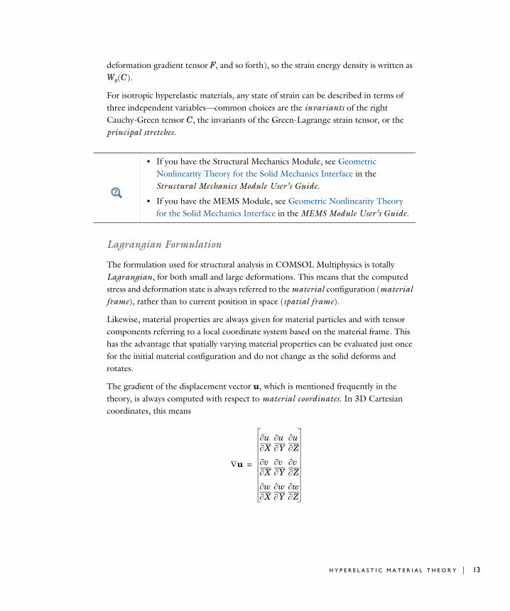
The gradient of the displacement vector u, which is mentioned frequently in the theory, is always computed with respect to material coordinates. In 3D Cartesian coordinates, this means

• If you have the Structural Mechanics Module, see Geometric Nonlinearity Theory for the Solid Mechanics Interface in the Structural Mechanics Module User’s Guide.

• If you have the MEMS Module, see Geometric Nonlinearity Theory for the Solid Mechanics Interface in the MEMS Module User’s Guide.

u

Xu

Yu

Zu

Xv

Yv

Zv

Xw

Yw

Zw

=

H Y P E R E L A S T I C M A T E R I A L T H E O R Y | 13

14 | C H A P T E R

The displacement is considered as a function of the material coordinates (X, Y, Z), but it is not explicitly a function of the spatial coordinates (x, y, z). It is thus only possible to compute derivatives with respect to the material coordinates.

Modeling Large Deformations

Consider a certain physical particle, initially located at the coordinate X. During deformation, this particle follows a path

Here, x is the spatial coordinate and X is the material coordinate.

For simplicity, assume that undeformed and deformed positions are measured in the same coordinate system. Using the displacement u it is then possible to write

The deformation gradient tensor F shows how an infinitesimal line element, dX, is mapped to the corresponding deformed line element dx by

The deformation gradient F contains the complete information about the local straining and rotation of the material. It is a two-point tensor (or a double vector), which transforms as a vector with respect to each of its indices. It involves both the reference and present configurations.

In terms of the displacement gradient, F can be written as

The deformation of the material (stretching) causes changes in the material density. The ratio between current and initial volume (or mass density) is given by

Here, 0 is the initial density and is the current density after deformation. The determinant of the deformation gradient tensor F is related to volumetric changes with

x x X t =

x X u X t +=

dx xX

-------dX F dX= =

F xX

------- u I+= =

dVdV0----------

0------ det F J= = =


respect to the initial state. A pure rigid body rotation implies J1, also, an incompressible material is represented by J1. These are called isochoric processes.

Since the deformation tensor F is a two-point tensor, it combines both spatial and material frames. It is not symmetric. Applying a singular value decomposition on the deformation gradient tensor gives an insight into how much stretch and rotation a unit volume of material has suffered. The right polar decomposition is defined as

where R is a proper orthogonal tensor ( , and ), and U is the right stretch tensor given in the material frame.

The right Cauchy-Green deformation tensor C defined by

is a symmetric and positive definite tensor, which accounts for the strain but not for the rotation. Also, the Green-Lagrange strain tensor is a symmetric tensor

The determinant of the deformation gradient tensor is always positive (a negative mass density is unphysical). The relation 0/J implies that for J1 there is compression, and for J1 there is elongation. Note that J0, so F is invertible. The variable solid.rho represents a “reference” or “initial” density 0, and not the “current” density .

F RU=

det R 1= R 1– RT=

The internal variables for the deformation gradient tensor are named solid.FdxX, solid.FdxY, and so on; for the rotation tensor they are named solid.RotxX, solid.RotxY, and so on; and for the right stretch tensor solid.UstchXX, solid.UstchXY, and so on. An upper case index refers to the material frame, and a lower case index refers to the spatial frame.

C FTF U2= =

12--- C I– =


16 | C H A P T E R

Some authors prefer to use the left Cauchy-Green deformation tensor BFFT, which is also symmetric and positive definite but it is defined in the spatial frame.

Modeling Elastic Deformations

The elastic deformation tensor is the basis for all strain energy formulations in hyperelastic materials and it is derived by removing the inelastic deformation from the total deformation tensor.

Normally, the total deformation is multiplicatively decoupled into elastic and inelastic deformations

The elastic deformation tensor is computed as

(2-1)

so the inelastic deformations are removed from the deformation gradient tensor. The elastic right Cauchy-Green deformation tensor is then computed from the elastic deformation gradient

and the elastic Green-Lagrange strain tensor is computed as:

The internal variables for the right Cauchy-Green deformation tensor in local coordinate system are named solid.Cl11, solid.Cl12, and so on; and for the Green-Lagrange strain tensor in local coordinates solid.el11, solid.el12, and so on.

F FelFin=

Fel FFin1–

=

Cel FelT Fel=

el12--- Cel I– =


The inelastic deformation tensor Fin is derived from inelastic processes, such as thermal expansion or plasticity.

Furthermore, the elastic, inelastic, and total volume ratio are related as

or

Thermal Expansion

If thermal expansion is present, a stress-free volume change occurs. This is a pure volumetric change, so the multiplicative decomposition of the deformation tensor in Equation 2-1 implies

Here, the thermal volume ratio, Jth, depends on the thermal stretch th, which for linear thermal expansion in isotropic materials can be written in terms of the isotropic coefficient of thermal expansion, iso, and the absolute change in temperature

and

Here, the term isoTTrefis the thermal strain. The isotropic thermal gradient is therefore a diagonal tensor defined as FththI.

The internal variables for the elastic right Cauchy-Green deformation tensor in the local coordinate system are named solid.Cel11, solid.Cel12, and so on; and for the elastic Green-Lagrange tensor in local coordinates solid.eel11, solid.eel12, and so on.

det F det Fel det Fin = J JelJin=

The internal variables for the elastic, inelastic, and total volume ratio are named solid.Jel, solid.Ji, and solid.J.

Jeldet F

det Fth --------------------- J

Jth--------= =

Jth th3= th 1 iso T Tref– +=

The internal variables for the thermal stretch and the thermal volume ratio are named solid.stchth, and solid.Jth.


18 | C H A P T E R

Large Strain Plasticity Theory

When large strain plasticity occurs, the plastic deformation gradient in not necessarily a diagonal tensor, as when thermal expansion occurs. The multiplicative decomposition of the deformation gradient tensor in Equation 2-1 implies

Here, the plastic deformation tensor Fp depends on the plastic flow rule, yield function, and plastic potential.

Isochoric Elastic Deformation

It turns out to be convenient for some classes of hyperelastic materials to split the strain energy density into volumetric (also called dilatational) and isochoric (also called distortional or volume-preserving) contributions. The elastic deformation tensor is then multiplicatively decomposed into the volumetric and isochoric components

with Fevol as the volumetric elastic deformation (a diagonal tensor) and the isochoric elastic deformation gradient. Isochoric deformation means that the volume ratio is kept constant during deformation, so the isochoric elastic deformation is computed by scaling it by the elastic volume ratio. The elastic volume ratio is defined by

and the volumetric deformation as

By using Jel it is possible to define the isochoric-elastic deformation gradient

the isochoric-elastic right Cauchy-Green tensor

Fel FFp 1–

=

Plastic Flow for Large Strains

Fel FevolFel=

Fel

Jel det Fel det Fevol = =

Fevol Jel1 3 I=

Fel Jel 1/3– Fel=


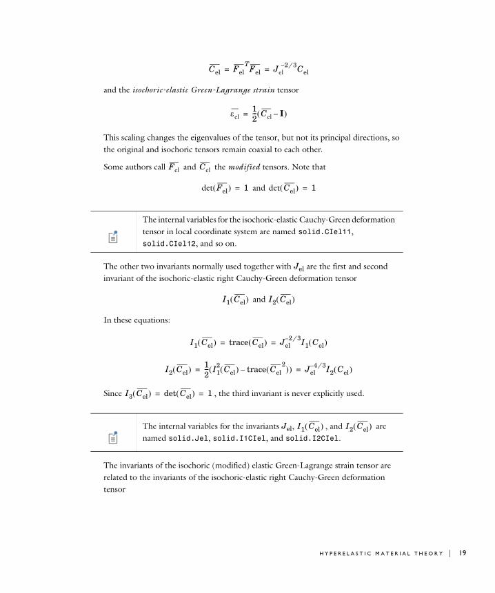
and the isochoric-elastic Green-Lagrange strain tensor

This scaling changes the eigenvalues of the tensor, but not its principal directions, so the original and isochoric tensors remain coaxial to each other.

Some authors call and the modified tensors. Note that

and

The other two invariants normally used together with Jel are the first and second invariant of the isochoric-elastic right Cauchy-Green deformation tensor

and

In these equations:

Since , the third invariant is never explicitly used.

The invariants of the isochoric (modified) elastic Green-Lagrange strain tensor are related to the invariants of the isochoric-elastic right Cauchy-Green deformation tensor

Cel FelT

Fel Jel 2/3– Cel= =

el12--- Cel I– =

Fel Cel

det Fel 1= det Cel 1=

The internal variables for the isochoric-elastic Cauchy-Green deformation tensor in local coordinate system are named solid.CIel11, solid.CIel12, and so on.

I1 Cel I2 Cel

I1 Cel trace Cel Jel2/3– I1 Cel = =

I2 Cel 12--- I1

2 Cel trace Cel2

– Jel4/3– I2 Cel = =

I3 Cel det Cel 1= =

The internal variables for the invariants Jel, , and are named solid.Jel, solid.I1CIel, and solid.I2CIel.

I1 Cel I2 Cel


20 | C H A P T E R

Nearly Incompressible Hyperelastic Materials

As mentioned in Working with Hyperelastic Materials, isotropic hyperelastic materials are described by their elastic strain energy density, Ws, written in terms of at most three independent variables. Common choices are the invariants of the elastic right Cauchy-Green tensor, the elastic Green-Lagrange strain tensor, the isochoric variants of these tensors, or the principal elastic stretches.

Once the strain energy density is defined, the second Piola-Kirchhoff stress in the local coordinate system is computed as

In the general case, the expression for the energy Ws is symbolically evaluated down to the components of C using the invariants definitions prior to the calculations of the components of the second Piola-Kirchhoff stress tensor. The differentiation is performed in components on the local coordinate system.

If the Nearly incompressible material check box is selected for the Hyperelastic Material node, the total elastic energy function is presented as:

where Wiso is the isochoric strain energy density and Wvol is the volumetric strain energy density.

I1 el trace el 12--- I1 Cel 3– = =

I2 el 12--- I1

2 el trace el2 – 1

4--- I2 Cel 2I1 Cel – 3+ = =

I3 el det el 18--- I1 Cel I2 Cel – = =

The internal variables for the invariants of the isochoric elastic Green-Lagrange strain tensor are named solid.I1eIel, solid.I2eIel, and solid.I3eIel.

S 2C

Ws=

Ws Wiso Wvol+=


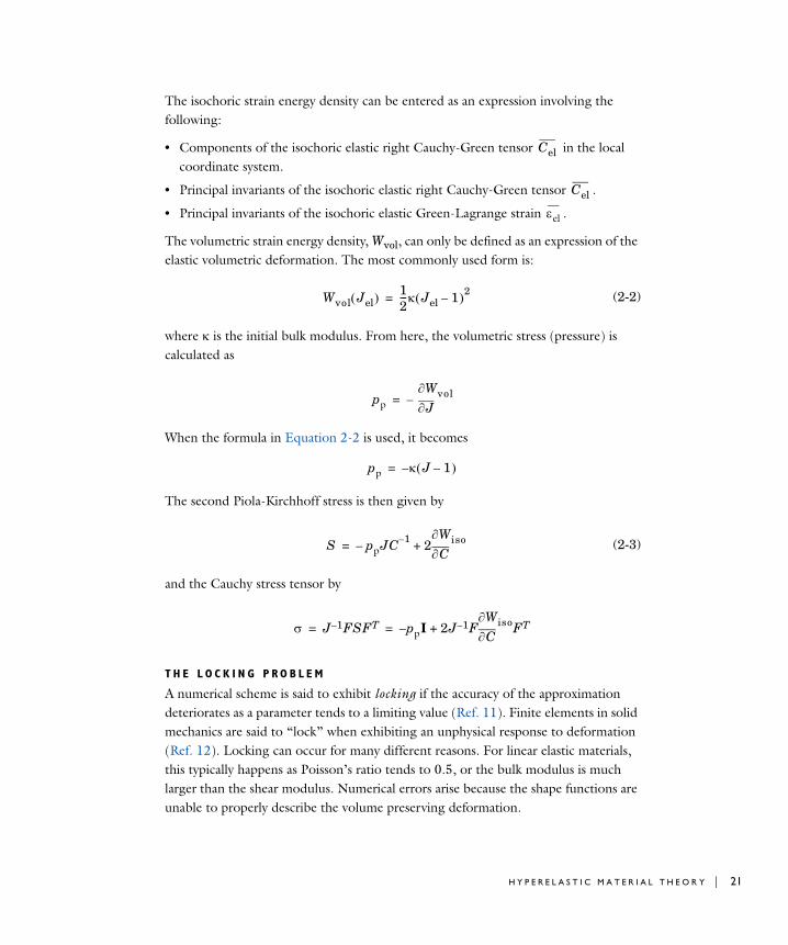
The isochoric strain energy density can be entered as an expression involving the following:

• Components of the isochoric elastic right Cauchy-Green tensor in the local coordinate system.

• Principal invariants of the isochoric elastic right Cauchy-Green tensor .

• Principal invariants of the isochoric elastic Green-Lagrange strain .

The volumetric strain energy density, Wvol, can only be defined as an expression of the elastic volumetric deformation. The most commonly used form is:

(2-2)

where is the initial bulk modulus. From here, the volumetric stress (pressure) is calculated as

When the formula in Equation 2-2 is used, it becomes

The second Piola-Kirchhoff stress is then given by

(2-3)

and the Cauchy stress tensor by

T H E L O C K I N G P R O B L E M

A numerical scheme is said to exhibit locking if the accuracy of the approximation deteriorates as a parameter tends to a limiting value (Ref. 11). Finite elements in solid mechanics are said to “lock” when exhibiting an unphysical response to deformation (Ref. 12). Locking can occur for many different reasons. For linear elastic materials, this typically happens as Poisson’s ratio tends to 0.5, or the bulk modulus is much larger than the shear modulus. Numerical errors arise because the shape functions are unable to properly describe the volume preserving deformation.

Cel

Cel

el

Wvol Jel 12--- Jel 1– 2=

pp JWvol–=

pp J 1– –=

S ppJC 1–– 2

CWiso+=

J 1– FSFT p– pI 2J 1– FC

WisoFT+= =


22 | C H A P T E R

To avoid the locking problem in computations, the mixed formulation replaces pp in Equation 2-3 with a corresponding interpolated pressure help variable pw, which adds extra degrees of freedom to the ones defined by the displacement vector u.

The general procedure is the same as when the Nearly incompressible material check box is selected for the Linear Elastic Materials node.

Theory for the Predefined Hyperelastic Material Models

Different hyperelastic material models are constructed by specifying different elastic strain energy expressions. This module has several predefined material models and also has the option to enter user-defined expressions for the strain energy density.

N E O - H O O K E A N

The strain energy density for the compressible version of the Neo-Hookean material is written in terms of the elastic volume ratio Jel and the first invariant of the elastic right Cauchy-Green deformation tensor I1Cel (Ref. 10).

Here, and are the Lamé coefficients. Note that the natural logarithm is used.

The nearly incompressible version uses the isochoric invariant and the initial bulk modulus

S T VE N A N T - K I R C H H O F F

One of the simplest hyperelastic material models is the St Venant-Kirchhoff material, which is an extension of a linear elastic material into the hyperelastic regime.

The elastic strain energy density is written with two parameters (the two Lamé coefficients) and two invariants of the elastic Green-Lagrange strain tensor, I1el and I2el

Here, and are the Lamé parameters.

Ws12--- I 1 3– Jel log–

12--- Jel log 2+=

I1 Cel

Ws12--- I1 3– 1

2--- Jel 1– 2+=

Ws12--- 2+ I1

2 2I2–=


The nearly incompressible version uses the isochoric invariants and , and the initial bulk modulus is calculated from the Lamé parameters

M O O N E Y - R I V L I N , TW O P A R A M E T E R S

Only a nearly incompressible version is available, and the elastic strain energy density is written in terms of the two isochoric invariants of the elastic right Cauchy-Green deformation tensors and , and the elastic volume ratio Jel

The material parameters C10 and C01 are related to the Lamé parameter C10C01

M O O N E Y - R I V L I N , F I V E P A R A M E T E R S

Rivlin and Saunders (Ref. 2) proposed a phenomenological model for small deformations in rubber-based materials on a polynomial expansion of the first two invariants of the elastic right Cauchy-Green deformation, so the strain energy density is written as an infinite series

with C00. This material model is sometimes also called polynomial hyperelastic material.

In the first-order approximation, the material model recovers the Mooney-Rivlin strain energy density

while the second-order approximation incorporates second-order terms

The nearly incompressible version uses the isochoric invariants of the elastic right Cauchy-Green deformation tensors

I1 el I2 el

Ws12--- 2+ I1

2 2I2–12--- Jel 1– 2+=

I1 Cel I2 Cel

Ws C10 I1 3– C01 I2 3– 12--- Jel 1– 2+ +=

Ws Cmn I1 3– m I2 3– n

n 0=

m 0=

=

Ws C10 I1 3– C01 I2 3– +=

Ws C10 I1 3– C01 I2 3– C20 I1 3– 2 C02 I2 3– 2 C11 I1 3– I2 3– + + + +=


24 | C H A P T E R

and

and it adds a contribution due to the elastic volume ratio. The strain energy density is then computed from

Here, is the initial bulk modulus.

M O O N E Y - R I V L I N , N I N E P A R A M E T E R S

The Mooney-Rivlin, nine parameters material model is an extension of the polynomial expression to third order terms and the strain energy density is written as

YE O H

Yeoh proposed (Ref. 1) a phenomenological model in order to fit experimental data of filled rubbers, where Mooney-Rivlin and Neo-Hookean models were to simple to describe the stiffening effect in the large strain regime. The strain energy was fitted to experimental data by means of three parameters, and the first invariant of the elastic right Cauchy-Green deformation tensors I1Cel

Since the shear modulus depends on the deformation, and it is calculated as

this imposes a restriction on the coefficients , since .

The nearly incompressible version uses the isochoric invariant of the elastic right Cauchy-Green deformation tensor , and it adds a contribution from the elastic volume ratio

I1 Cel I2 Cel

Ws Cmn I1 3– m I2 3– n 12--- Jel 1– 2+

n 0=

2

m 0=

2

=

Ws Cmn I1 3– m I2 3– n 12--- Jel 1– 2+

n 0=

3

m 0=

3

=

Ws c1 I1 3– c2 I1 3– 2 c3 I1 3– 3+ +=

2I1

Ws

I2Ws+

2c1 4c2 I1 3– 6c3 I1 3– 2+ += =

c1 c2 c3 0

I1 Cel

Ws c1 I1 3– c2 I1 3– 2 c3 I1 3– 3 12--- Jel 1– 2+ + +=


O G D E N

The Neo-Hookean material model usually fits well to experimental data at moderate strains, but fails to model hyperelastic deformations at high strains. In order to model rubber-like materials at high strains, Ogden adapted (Ref. 1) the energy of a Neo-Hookean material to

Here p and p are material parameters, and el1, el2, and el3 are the principal elastic stretches such as Jelel1el2el3.

The Ogden model is empirical, in the sense that it does not relate the material parameters p and p to physical phenomena. The parameters p and p are obtained by curve-fitting measured data, which can be difficult for N. The most common implementation of Ogden material is with N, so four parameters are needed.

The nearly incompressible version uses the isochoric elastic stretches

and the initial bulk modulus

The isochoric elastic stretches define a volume preserving deformation, since

S T O R A K E R S

The Storakers material (Ref. 12 and Ref. 15) is commonly used to model highly compressible foams. The strain energy density is written in a similar fashion as in Ogden material:

The initial shear and bulk moduli can be computed from the parameters k and k as

Wspp------ el1

p el2p el3

p 3–+ +

p 1=

N

=

eli eli Jel1 3=

Wspp------ el1

p el2p el3

p 3–+ +

p 1=

N

12--- Jel 1– 2+=

el1el2el3 el1el2el3 Jel 1= =

Ws2k

k2

--------- el1k el2

k el3k 3–

1k----- Jel

k– k 1– + + +

k 1=

N

=


26 | C H A P T E R

2

and

for constantparameters k, the initial bulk modulus becomes , so a stable material requires and . In this case, the Poisson's ratio is given by , which means that for a Poisson’s ratio bigger than is needed.

VA R G A

The Varga material model (Ref. 1) describes the strain energy in terms of the elastic stretches as

The nearly incompressible version uses the isochoric elastic stretches defined as

and the initial bulk modulus

The simplest Varga model is obtained by setting c1 and c2

A R R U D A - B O Y C E

The other hyperelastic materials described are phenomenological models in the sense that they do not relate the different material parameters (normally obtained by curve-fitting experimental data) to physical phenomena.

Arruda and Boyce (Ref. 3) derived a material model based on Langevin statistics of polymer chains. The strain energy density is defined by

k

k 1=

N

= 2k k13---+

k 1=

N

=

Ws c1 el1 el2 el3 3–+ + c2 el1el2 el2el3 el1el3 3–+ + +=

eli eli Jel1 3=

Ws c1 el1 el2 el3 3–+ + c2 el1el2 el2el3 el1el3 3–+ + 12--- Jel 1– + +=

Ws el1 el2 el3 3–+ + 12--- Jel 1– 2+=

Ws 0 cp I1p 3p

–

p 1=

=


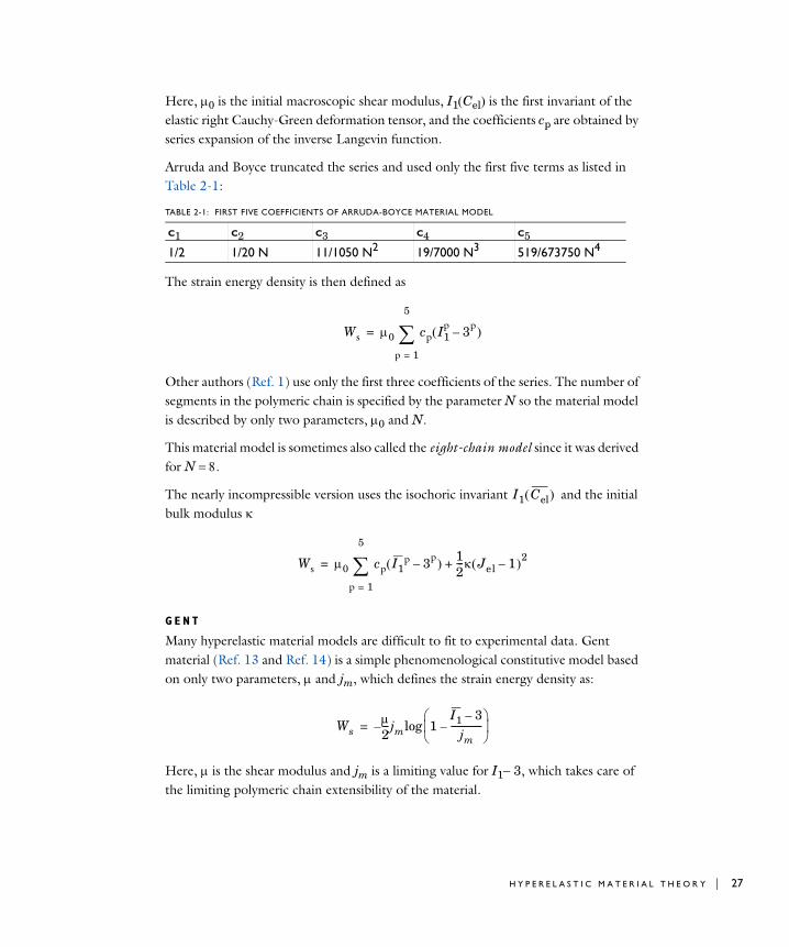
Here, 0 is the initial macroscopic shear modulus, I1Cel is the first invariant of the elastic right Cauchy-Green deformation tensor, and the coefficients cp are obtained by series expansion of the inverse Langevin function.

Arruda and Boyce truncated the series and used only the first five terms as listed in Table 2-1:

The strain energy density is then defined as

Other authors (Ref. 1) use only the first three coefficients of the series. The number of segments in the polymeric chain is specified by the parameter N so the material model is described by only two parameters, 0 and N.

This material model is sometimes also called the eight-chain model since it was derived for N.

The nearly incompressible version uses the isochoric invariant and the initial bulk modulus

G E N T

Many hyperelastic material models are difficult to fit to experimental data. Gent material (Ref. 13 and Ref. 14) is a simple phenomenological constitutive model based on only two parameters, and jm, which defines the strain energy density as:

Here, is the shear modulus and jm is a limiting value for I13, which takes care of the limiting polymeric chain extensibility of the material.

TABLE 2-1: FIRST FIVE COEFFICIENTS OF ARRUDA-BOYCE MATERIAL MODEL

C1 C2 C3 C4 C5

1/2 1/20 N 11/1050 N2 19/7000 N3 519/673750 N4

Ws 0 cp I1p 3p

–

p 1=

5

=

I1 Cel

Ws 0 cp I1p 3p

–

p 1=

5

12--- Jel 1– 2+=

Ws2---– jm 1

I1 3–

jm--------------–

log=


28 | C H A P T E R

Since the strain energy density does not depend on the second invariant I2, the Gent model is often classified as a generalized Neo-Hookean material. The strain energy density tends to be the one of incompressible Neo-Hookean material as .

The nearly incompressible formulation uses the isochoric invariants and the initial bulk modulus

Gent material is the simplest model of the limiting chain extensibility family.

B L A T Z - K O

The Blatz-Ko material model was developed for foamed elastomers and polyurethane rubbers, and it is valid for compressible isotropic hyperelastic materials (Ref. 1).

The elastic strain energy density is written with three parameters and the three invariants of the elastic right Cauchy-Green deformation tensor, I1Cel, I2Cel, and I3Cel

Here, is an interpolation parameter bounded to , µ is the shear modulus, and is an expression of Poisson’s ratio.

When the parameter , the strain energy simplifies to a similar form of the Mooney-Rivlin material model

In the special case of , the strain energy reduces to a similar form of the Neo-Hookean model

G A O

Gao proposed (Ref. 16) a simple hyperelastic material where the strain energy density is defined by two parameters, a and n, and two invariants of the elastic right Cauchy-Green deformation tensors Cel:

jm

I1 Cel

Ws2---– jm 1

I1 3–

jm--------------–

log 12--- Jel 1– 2+=

Ws 2--- I1 3– 1

--- I3

– 1– + 1 –

2---

I2I3----- 3– 1

--- I3

1– + +=

Ws 2--- I1 3– 1 –

2---

I2I3----- 3– +=

Ws2--- I1 3–

2------ J 2– 1– +=


Here, the invariant I-1Celis calculated as:

Gao proposed that the material is unconditionally stable when the parameters are bounded to n and a, and related these parameters under small strain to the Young’s module and Poisson’s ratio by:

and

Since n and it is bounded to n, this material model is stable for materials with an initial Poisson’s ratio in the range of

M U R N A G H A N

The Murnaghan potential is used in nonlinear acoustoelasticity. Most conveniently it is expressed in terms of the three invariants of the elastic Green-Lagrange strain tensor, I1el, I2el, and I3el

Here, l, m, and n are the Murnaghan third-order elastic moduli, which can be found experimentally for many commonly encountered materials such as steel and aluminum, and and are the Lamé parameters.

U S E R D E F I N E D

When a material model is user-defined, an expression for the elastic strain energy Ws is entered, which can include any expressions involving the following:

• Components of Cel, the elastic right Cauchy-Green deformation tensor in the local material coordinate system.

• Principal invariants of Cel

Ws a I1n I 1–

n+ =

I 1– trace Cel1–

I2 Cel I3 Cel ------------------= =

E 3nn28a2n 1+

--------------------= n 1–2n 1+-----------------=

Ws12--- 2+ I1

2 2I2–13--- l 2m+ I1

3 2mI1I2– nI3+ +=

I1 Cel trace Cel =

I2 Cel 12--- I1

2 Cel trace Cel2 – =


30 | C H A P T E R

• Components of the elastic Green-Lagrange strain tensor elin the local coordinate system.

• Principal elastic stretches el1, el2, and el3, which are the square-root of the eigenvalues of the elastic right Cauchy-Green deformation tensor Cel.

• Invariants of the elastic Green-Lagrange strain tensor. Since

the invariants of el are written in terms of the invariants of Cel:

• When the Nearly incompressible material check box is selected for the Hyperelastic Material node, the elastic strain energy is decoupled into the volumetric and isochoric components.

Enter the volumetric strain energy Wvol, which can be an expression involving the elastic volume ratio

I3 Cel det Cel =

The internal variables for these invariants are named solid.I1Cel, solid.I2Cel, and solid.I3Cel.

The internal variables for the principal elastic stretches are named solid.stchelp1, solid.stchelp2, and solid.stchelp3.

el12--- Cel I– =

I1 el trace el 12--- I1 Cel 3– = =

I2 el 12--- I1

2 el trace el2 – 1

4--- I2 Cel 2I– 1 Cel 3+ = =

I3 el det el 18--- I3 Cel I– 2 Cel I+

1Cel 1– = =

The internal variables for these invariants are named solid.I1eel, solid.I2eel, and solid.I3eel.


Also enter the isochoric strain energy, Wiso, as an expression involving the invariants of the isochoric elastic right Cauchy-Green tensor

and

or the invariants of the isochoric elastic Green-Lagrange strain

, , and

Jel det Fel =

I1 Cel I2 Cel

I1 el I2 el I3 el

The internal variables for Jel, , and are named solid.Jel, solid.I1CIel, and solid.I2CIel.

The internal variables for , , and are named solid.I1eIel, solid.I2eIel, and solid.I3eIel.

The strain energy density must not contain any other expressions involving displacement or their derivatives. This excludes components of the displacement gradient u and deformation gradient FuI tensors, their transpose, inversions, as well as the global material system components of C and . If they occur, such variables are treated as constants during symbolic differentiations.

I1 Cel I2 Cel

I1 el I2 el I3 el


32 | C H A P T E R

E l a s t o p l a s t i c Ma t e r i a l T h e o r y

In this section:

• Introduction to Small and Large Plastic Strains

• Plastic Flow for Small Strains

• Isotropic Plasticity

• Yield Function

• Hill Orthotropic Plasticity

• Hardening Models

• Plastic Flow for Large Strains

• Numerical Solution of the Elastoplastic Conditions

• References for Elastoplastic Materials

Introduction to Small and Large Plastic Strains

There are two implementations of plasticity available in COMSOL Multiphysics. One is based on the additive decomposition of strains, which is the most suitable approach in the case of small strains, and the other one is based on the multiplicative decomposition of the deformation gradient, which is more suitable when large plastic strains occurs.

The additive decomposition of strains is used when small plastic strain is selected as the plasticity model. The stress-strain relationship is then written as

Here:

• is the Cauchy stress tensor

• is the total strain tensor

• 0 and 0 are the initial stress and strain tensors

Working with Nonlinear Structural Materials

0– C: 0– th– p– c– =


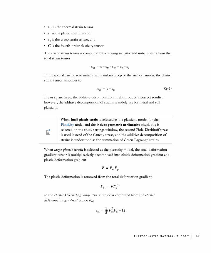
• th is the thermal strain tensor

• p is the plastic strain tensor

• c is the creep strain tensor, and

• C is the fourth-order elasticity tensor.

The elastic strain tensor is computed by removing inelastic and initial strains from the total strain tensor

In the special case of zero initial strains and no creep or thermal expansion, the elastic strain tensor simplifies to

(2-4)

If or p are large, the additive decomposition might produce incorrect results; however, the additive decomposition of strains is widely use for metal and soil plasticity.

When large plastic strain is selected as the plasticity model, the total deformation gradient tensor is multiplicatively decomposed into elastic deformation gradient and plastic deformation gradient

The plastic deformation is removed from the total deformation gradient,

so the elastic Green-Lagrange strain tensor is computed from the elastic deformation gradient tensor Fel

el 0– th– p– c–=

el p–=

When Small plastic strain is selected as the plasticity model for the Plasticity node, and the Include geometric nonlinearity check box is selected on the study settings window, the second Piola-Kirchhoff stress is used instead of the Cauchy stress, and the additive decomposition of strains is understood as the summation of Green-Lagrange strains.

F FelFp=

Fel FFp 1–

=

el12--- Fel

T Fel I– =

E L A S T O P L A S T I C M A T E R I A L T H E O R Y | 33

34 | C H A P T E R

and the plastic Green-Lagrange strain tensor is computed from the plastic deformation gradient tensor

As opposed to the small strain formulation described in Equation 2-4, the total, plastic and elastic Green-Lagrange strain tensors are related as

Under multiplicative decomposition, the elastic right Cauchy-Green tensor and the plastic right Cauchy-Green tensor are defined as

and

Plastic Flow for Small Strains

The flow rule defines the relationship between the increment of the plastic strain tensor and the current state of stress, for a yielded material subject to further loading. When Small plastic strain is selected as the plasticity model for the Plasticity node, the direction of the plastic strain increment is defined by

Here, is a positive multiplier (also called the consistency parameter or plastic multiplier) which depends on the current state of stress and the load history, and Qp is the plastic potential.

p12--- Fp

TFp I– =

el FpT– p– Fp

1–=

Cel FelT Fel= Cp Fp

TFp=

When Large plastic strain is selected as the plasticity model for the Plasticity node, the Include geometric nonlinearity check box in the study settings is automatically selected and becomes unavailable.

·p

·p Qp

----------=

The “dot” (for ) means the rate at which the plastic strain tensor changes with respect to Qp/. It does not represent a true time derivative. Some authors call this formulation rate independent plasticity.

·p


The direction of the plastic strain increment is perpendicular to the surface (in the space of principal stresses) defined by the plastic potential Qp.

The plastic multiplier is determined by the complementarity or Kuhn-Tucker conditions

, and (2-5)

where Fy is the yield function. The yield surface encloses the elastic region defined by Fy<0. Plastic flow occurs when Fy=0.

If the plastic potential and the yield surface coincide with each other Qp=Fy, the flow rule is called associated, and the rate in Equation 2-6 is solved together with the conditions in Equation 2-5.

(2-6)

For a non-associated flow rule, the yield function does not coincide with the plastic potential, and together with the conditions in Equation 2-5, the rate in Equation 2-7 is solved for the plastic potential Qp (often, a smoothed version of Fy).

(2-7)

The evolution of the plastic strain tensor (with either Equation 2-6 or Equation 2-7, plus the conditions in Equation 2-5) is implemented at Gauss points in the plastic element elplastic.

Isotropic Plasticity

For isotropic plasticity, the plastic potential Qp is written in terms of at most three invariants of Cauchy’s stress tensor

where the invariants of the stress tensor are

·p

0 Fy 0 Fy 0=

·p Fy---------=

·p Qp

----------=

·p

Qp Qp I1 J2 J3 =

I1 trace =

J2 12---dev :dev =

J3 det dev =


36 | C H A P T E R

so that the increment of the plastic strain tensor can be decomposed into

The increment in the plastic strain tensor includes in a general case both deviatoric and volumetric parts. The tensor is symmetric given the following properties

(2-8)

A common measure of inelastic deformation is the effective plastic strain rate, which is defined as

(2-9)

The trace of the incremental plastic strain tensor, which is called the volumetric plastic strain rate , depends only on the reliance of the plastic potential on the first invariant I1(), sinceJ2/ and J3/ are deviatoric tensors

For metal plasticity under the von Mises and Tresca criteria, the volumetric plastic strain rate is always zero because the plastic potential is independent of the invariant I1. This is known as J2 plasticity.

·p

·p Qp

---------- QpI1----------

I1--------

QpJ2----------

J2---------

QpJ3----------

J3---------+ +

= =

·p

·p

I1-------- I=

J2--------- dev =

J3--------- dev dev 2

3---J2I–=

·pe23---·p:·p=

·pvol

·pvol trace ·p traceQp

---------- 3

QpI1----------= = =

Plasticity

The effective plastic strain and the volumetric plastic strain are available in the variables solid.epe and solid.epvol.


Yield Function

When an associated flow rule is applied, the yield function must be smooth, that is, continuously differentiable with respect to the stress. In COMSOL Multiphysics, the following form is used:

where ys is the yield stress.

The predefined form of the effective stress is the von Mises stress, which is commonly used in metal plasticity:

Other expressions can be defined, such as Tresca stress, Hill orthotropic plasticity, or another user-defined expression.

The Tresca effective stress is calculated from the difference between the largest and the smallest principal stress

A user-defined yield function can by expressed in terms of invariants of the stress tensor such as the pressure (volumetric stress)

the effective (von Mises) stress mises, or other invariants, principal stresses, or stress tensor components.

Hill Orthotropic Plasticity

Hill (Ref. 4, Ref. 5) proposed a quadratic yield function (and associated plastic potential) in a local coordinate system given by the principal axes of orthotropy ai

Fy ys–=

mises 3J2 32---dev :dev = =

tresca 1 3–=

p 13---– I1 =

Plasticity


38 | C H A P T E R

(2-10)

The six parameters F, G, H, L, M, and N are related to the state of anisotropy. As with isotropic plasticity, the elastic region Qp0 is bounded by the yield surface Qp0.

Hill demonstrated that this type of anisotropic plasticity is volume preserving, this is, given the associated flow rule

the trace of the plastic strain rate tensor is zero, which follows from the expressions for the diagonal elements of

so the plastic volumetric strain rate is zero

E X P R E S S I O N S F O R T H E C O E F F I C I E N T S F , G , H , L , M , N

Hill noticed that the parameters L, M, and N are related to the yield stress in shear with respect to the axes of orthotropy ai, thus they are positive parameters

, ,

Qp F 22 33– 2 G 33 11– 2 H 11 22– 2+ + +=

2L232 2M31

2 2N122 1–+ +

·p Qp

----------=

·p

·p11 Qp11------------ 2 G– 33 11– H 11 22– + = =

·p22 Qp22------------ 2 F 22 33– H– 11 22– = =

·p33 Qp33------------ 2 F– 22 33– G 33 11– + = =

·pvol trace ·p ·p11 ·p22 ·p33+ + 0= = =

Hill plasticity is an extension to J2 (von Mises) plasticity, in the sense that it is volume preserving. Due to this assumption, six parameters are needed to define orthotropic plasticity, as opposed to orthotropic elasticity, where nine elastic coefficients are needed.

L 1

2ys232

----------------= M 1

2ys312

----------------= N 1

2ys122

----------------=


Here, ysij represents the yield stress in shear on the plane ij.

The material parameters ys1, ys2, and ys3 represent the tensile yield stress in the direction, a1, a2, and a3, and they are related to Hill’s parameters F, G, and H as

or equally

Note that at most, only one of the three coefficients F, G, and H can be negative.

In order to define a yield function and plastic potential suitable for isotropic or kinematic hardening, the average initial yield stress ys0 is calculated from the Hill’s parameters F, G, and H (this is equivalent to the initial yield stress ys0 in von Mises plasticity)

(2-11)

Defining Hill’s effective stress as (Ref. 5)

makes it possible to write the plastic potential in a similar way to von Mises plasticity.

Hardening is then applied on the average yield stress variable ys0, by using the plastic potential

Here, the average yield stress

1

ys12

---------- G H+=

1

ys22

---------- H F+=

1

ys32

---------- F G+=

2F 1

ys22

---------- 1

ys32

---------- 1

ys12

----------–+=

2G 1

ys32

---------- 1

ys12

---------- 1

ys22

----------–+=

2H 1

ys12

---------- 1

ys22

---------- 1

ys32

----------–+=

In case of hardening, these coefficients (either Hill’s coefficients or the shear and tensile yield stresses) are renamed with the “initial” prefix.

1

ys02

----------- 23--- F G H+ + 1

3--- 1

ys12

---------- 1

ys22

---------- 1

ys32

----------+ +

= =

hill2 ys0

2 F 22 33– 2 G 33 11– 2 H 11 22– 2+ +=

2+ L232 M31

2 N122

+ +

Qp hill ys–=


40 | C H A P T E R

now depends on the initial yield stress ys0, the hardening function h, and the effective plastic strain pe.

Hardening Models

The plasticity model implements three different kinds of hardening models for elastoplastic materials:

• Perfect plasticity (no hardening)

• Isotropic hardening

• Kinematic hardening

P E R F E C T ( O R I D E A L ) P L A S T I C I T Y

In this case the plasticity algorithm solves either the associated or non-associated flow rule for the plastic potential Qp

with the yield function

In the settings for plasticity you specify the effective stress for the yield function from a von Mises stress, a Tresca stress, Hill effective stress, or a user-defined expression.

ys ys0 h pe +=

Plasticity

·p Qp

----------=

Fy ys0–=

When Large plastic strain is selected as the plasticity model for the Plasticity node, either the associate or non-associated flow rule is applied as written in Equation 2-14.


I S O T R O P I C H A R D E N I N G

In this case the plasticity algorithm solves either the associated or non-associated flow rule for the plastic potential Qp

with the yield function

where pe is the effective plastic strain. The variable yspe is the yield stress, which now depends on the effective plastic strain. The yield stress versus the effective plastic strain can be specified in two different ways — tangent data (linear isotropic hardening), or hardening function data. When using hardening function data, the hardening curve could also depend on other variables, such as stress or temperature.

Tangent Data (Linear Isotropic Hardening)In this case, an isotropic tangent modulus ETiso is given. This tangent modulus is defined as (stress increment / total strain increment), and it relates the hardening to the effective plastic strain linearly. The yield stress yspe is a linear function of the effective plastic strain

with and

here, ys0 is the initial yield stress, and k is the isotropic hardening modulus. A value for ETiso is entered in the isotropic tangent modulus section for the Plasticity node. The Young’s modulus E is taken from the linear elastic material. For orthotropic and anisotropic elastic materials, E represents an average Young’s modulus.

Hardening Function DataIn this case, define the (usually nonlinear) hardening function hpe such that the yields stress reads

·p Qp

----------=

Fy ys pe –=

ys pe ys0 h pe +=

h pe kpe=1k--- 1

ETiso-------------- 1

E----–=


42 | C H A P T E R

K I N E M A T I C H A R D E N I N G

The algorithm solves either the associated or non-associated flow rule for the plastic potential Qp

with the yield function defined as

and

Here, ys0 is the initial yield stress, and the effective stress is either the von Mises stress or a user-defined expression. The stress tensor used in the yield function is shifted by what is usually called the back stress, shift.

The back stress is generally not only a function of the current plastic strain but also of its history. In the case of linear kinematic hardening, f p is a linear function of the plastic strain tensor p, this is also known as Prager’s hardening rule. The implementation of kinematic hardening assumes a linear evolution of the back stress tensor with respect to the plastic strain tensor:

ys pe ys0 h pe +=

This is the preferred way to define nonlinear hardening models.

The internal variable for the effective plastic strain is named solid.epe. The effective plastic strain evaluated at Gauss points is named solid.epeGp, where solid is the name of the interface identifier for the physics interface.

When Large plastic strain is selected as the plasticity model for the Plasticity node, either the associate or non-associated flow rule is applied as written in Equation 2-14.

·p Qp

----------=

Fy shift– ys0–= shift f p =

shift23---cp=


where the work hardening constant is calculated from

The value for ETkin is entered in the kinematic tangent modulus section and the Young’s modulus E is taken from the linear elastic material model. For orthotropic and anisotropic elastic materials, E represents an average Young’s modulus.

Plastic Flow for Large Strains

When Large plastic strain is selected as the plasticity model for the Plasticity node, a multiplicative decomposition of deformation (Ref. 4, Ref. 2, and Ref. 5) is used, and the associated plastic flow rule can be written as the Lie derivative of the elastic left Cauchy-Green deformation tensor Bel:

(2-12)

The plastic multiplier and the yield function (written in terms of the Kirchhoff stress tensor ) satisfy the Kuhn-Tucker condition, as done for infinitesimal strain plasticity

, and

The Lie derivative of Bel is then written in terms of the plastic right Cauchy-Green rate

1c--- 1

ETkin--------------- 1

E----–

=

When kinematic hardening is added, both the plastic potential and the yield surface are calculated with effective invariants, that is, the invariants of the tensor defined by the difference between the stress tensor minus the back-stress, . The invariant of effective deviatoric tensor is named solid.II2sEff, which is used when a von Mises plasticity is computed together with kinematic hardening.

eff shift–=

12---– L Bel

-------Bel=

0 0 0=

The yield function in Ref. 4 and Ref. 2 was written in terms of Kirchhoff stress and not Cauchy stress because the authors defined the plastic dissipation with the conjugate energy pair and d, where d is the rate of strain tensor.


44 | C H A P T E R

(2-13)

By using Equation 2-12 and Equation 2-13the either associated or non-associated plastic flow rule for large strains is written as (Ref. 2)

(2-14)

together with the Kuhn-Tucker conditions for the plastic multiplier and the yield function Fy

, and (2-15)

For the associated flow rule, the plastic potential and the yield surface coincide with each other (Qp=Fy), and for the non-associated case, the yield function does not coincide with the plastic potential.

In COMSOL Multiphysics, the elastic left Cauchy-Green tensor is written in terms of the deformation gradient and the right Cauchy-Green tensor, so Bel=FCp

1F. The plastic flow rule is then solved at Gauss points in the plastic element elplastic for the inverse of the plastic deformation gradient Fp

1, so that the variables in Equation 2-14 are replaced by

and

The flow rule then reads

(2-16)

After integrating the flow rule in Equation 2-16, the plastic Green-Lagrange strain tensor is computed from the plastic deformation tensor

and the elastic Green-Lagrange strain tensor is computed from the elastic deformation gradient tensor Fel=FFp

1

L Bel FCp1–· FT=

12---– FCp

1–· FT Qp

----------Bel=

0 Fy 0 Fy 0=

Cp1–· Fp

1–· FpT– Fp

1– FpT–·+= Bel FelFel

T FFp1– Fp

T– FT= =

12---– Fp

1–· FpT– Fp

1– FpT–·+ F 1–

Qp

----------FFp1– Fp

T–=

p12--- Fp

TFp I– =


Numerical Solution of the Elastoplastic Conditions

A backward Euler discretization of the pseudo-time derivative is used in the plastic flow rule. For small plastic strains, this gives

where old denotes the previous time step and , where t is the pseudo-time step length. For large plastic strains, Equation 2-16 gives

where .

For each Gauss point, the plastic state variables (p and M, respectively) and the plastic multiplier, , are computed by solving the above time-discretized flow rule together with the complementarity conditions

, and

This is done as follows (Ref. 4):

1 Elastic-predictor: Try the elastic solution (or ) and . If this satisfies it is done.

2 Plastic-corrector: If the elastic solution does not work (this is ), solve the nonlinear system consisting of the flow rule and the equation using a damped Newton method.

References for Elastoplastic Materials

1. J. Simo and T. Hughes, Computational Inelasticity, Springer, 1998.

el12--- Fel

T Fel I– =

When Large plastic strain is selected as the plasticity model for the Plasticity node, the effective plastic strain variable is computed as the true effective plastic strain (also called Hencky or logarithmic plastic strain).

p p,old– Qp

----------=

t=

12---F 2MMT MoldMT

– MMoldT

– – Qp

----------FMMT=

M Fp1–

=

0 Fy 0 Fy 0=

p p,old= M Mold= 0=

Fy 0

Fy 0Fy 0=


46 | C H A P T E R

2. J. Simo, “Algorithms for Static and Dynamic Multiplicative Plasticity that Preserve the Classical Return Mapping Schemes of the Infinitesimal Theory,” Computer Methods in Applied Mechanics and Engineering, vol. 99, pp. 61–112, 1992.

3. J. Lubliner, Plasticity Theory, Dover, 2008.

4. R. Hill, “A Theory of the Yielding and Plastic Flow of Anisotropic Metals,” Proc. Roy. Soc. London, vol. 193, pp. 281–297, 1948.

5. N. Ottosen and M. Ristinmaa, The Mechanics of Constitutive Modeling, Elsevier Science, 2005.


C r e e p and V i s c o p l a s t i c i t y T h e o r y

In this section:

• About Creep

• Fundamental Creep Material Models

• Creep Material Models for Metals and Crystalline Solids

• Viscoplasticity

• Solver Settings for Creep and Viscoplasticity

About Creep

Creep is an inelastic time-dependent deformation that occurs when a material is subjected to stress (typically much less than the yield stress) at sufficiently high temperatures.

The creep strain rate, in a general case, depends on stress, temperature, and time, usually in a nonlinear manner:

It is often possible to separate these effects as shown in this equation:

Working with Nonlinear Structural Materials

In the literature, the terms viscoplasticity and creep are often used interchangeably to refer to the class of problems related to rate-dependent plasticity.

·c Fcr T t =

Fcr t T f1 f2 T f3 t =

C R E E P A N D V I S C O P L A S T I C I T Y T H E O R Y | 47

48 | C H A P T E R

Experimental data shows three types of behavior for the creep strain rate at constant stress as function of time. Researchers normally subdivide the creep curve into three regimes, based on the fact that many different materials show similar responses:

• In the initial primary creep regime (also called transient creep) the creep strain rate decreases with time to a minimum steady-state value.

• In the secondary creep regime the creep strain rate is almost constant. This is also called steady-state creep.

• In the tertiary creep regime the creep strain increases with time until a failure occurs.

When this distinction is assumed, the total creep rate can be additively split into primary, secondary, and tertiary creep rates

In most cases, Fcr1 and Fcr3 depend on stress, temperature and time, while secondary creep, Fcr2, depends only on stress level and temperature. Normally, secondary creep

·c Fcr1 Fcr2 Fcr3+ +=


is the dominant process. Tertiary creep is seldom important because it only accounts for a small fraction of the total lifetime of a given material.

Figure 2-1: Uniaxial creep as a function of logarithmic time.

Fundamental Creep Material Models

Despite the fact that the creep response of a given material is related to its atomic structure, a macroscopic (continuum mechanics) description is normally appropriate for modeling scientific and engineering problems.

The fundamental mathematical models available for modeling creep are:

• Creep Potential

• Volumetric Creep

• Deviatoric Creep

• User-Defined Creep

c

1 >2

1

2

tertiary creepsecondary creep

primary creep

log time

Creep and Viscoplasticity


50 | C H A P T E R

These creep models are contributing subnodes to the Linear Elastic Material and they can also be combined with Plasticity and Thermal Expansion subnodes for more advanced models.

C R E E P PO T E N T I A L

Some authors use a creep potential to describe the secondary creep rate, so that the creep rate is written in a way similar to the flow rule for plasticity:

and

Here, Qcr is a user-defined creep potential, which is normally written in terms of invariants of the stress tensor.

Volumetric creep is obtained when the creep potential depends only on the first invariant of Cauchy stress tensor, I1, since

This is equivalent to that the creep potential would depend on the pressure pI1.

When the creep potential depends only on the second deviatoric invariant of Cauchy stress tensor, J2, the deviatoric creep model is obtained since

This is equivalent to that the creep potential would depend on the effective stress e3J2.

When (in SI units) the creep potential, Qcr, is given in units of Pa, the rate multiplier is given in units of 1/s.

• Creep and Viscoplasticity

• Plasticity

• See the Solid Mechanics interface in the Structural Mechanics Module User’s Guide or in the MEMS Module User’s Guide for details about the Thermal Expansion and Linear Elastic Material nodes.

·c Qcr

-----------= 0

Qcr

-----------QcrI1

-----------I=

Qcr

-----------QcrJ2-----------dev =


VO L U M E T R I C C R E E P

The creep strain rate is calculated by solving the rate equation

so the creep rate tensor is a diagonal tensor, and the trace of the creep rate tensor, the volumetric creep strain rate, equals the user input Fcr

(2-17)

The creep rate, Fcr, usually depends on the first invariant of Cauchy stress I1 or the pressure pI1, in addition to the temperature and other material parameters.

D E V I A T O R I C C R E E P


Here, nD is a deviatoric tensor coaxial to the stress tensor.

The creep rate, Fcr, normally depends on the second deviatoric invariant of the stress J2 or the effective or von Mises (effective) stress e, in addition to the temperature and other material parameters.

The deviatoric tensor nD is defined as

The resulting creep strain rate tensor is also deviatoric, since trace (nD)

Given the property

the effective creep strain rate equals the absolute value of the user input Fcr

·c13---FcrI=

trace ·c Fcr=

·c FcrnD=

nD 32---dev

e-----------------=

trace ·c Fcrtrace nD 0= =

nD:nD 32---=

·ce23---·c:

·c Fcr= =


52 | C H A P T E R

Deviatoric creep is very popular to model creep in metals and alloys. For example, Norton’s law is a deviatoric creep model.

U S E R - D E F I N E D C R E E P


where Fcr is a user-defined symmetric tensor field.

E N E R G Y D I S S I P A T I O N

Since creep is an inelastic process, the dissipated energy density can be calculated by integrating the creep dissipation rate density (SI unit: W/m3) given by

In case many creep sub-nodes are added to a Linear Elastic Material node, the creep dissipation rate density is calculated from the total creep strain rate tensor .

The total energy dissipated by creep in a given volume can be calculated by a volume integration of the dissipated creep energy density Wc (SI unit: J/m3).

The effective creep strain and the effective creep strain rate are available in the variables solid.ece and solid.ecet.

·c Fcr=

Potential, Volumetric, Deviatoric, or User defined creep do not overwrite each other. These are all contributing nodes to the Linear Elastic Material node.

W·

cdr :·c=

·c

When the Calculate dissipated energy check box is selected, the creep dissipation rate density is available under the variable solid.Wcdr and the dissipated creep energy density under the variable Wc.

• Creep

• Linear Elastic Material in the Structural Mechanics User’s Guide.


Solver Settings for Creep and Viscoplasticity

Creep and Viscoplasticity are time-dependent phenomena.

P H Y S I C S I N T E R F A C E S E T T I N G S

In the Model Builder, click the Solid Mechanics node. In the settings window, under Structural Transient Behavior, select Quasi-static to treat the elastic behavior as quasi-static (with no mass effects; that is, no second-order time derivatives for the displacement variables). Selecting this option gives a more efficient solution for problems where the variation in time is slow when compared to the natural frequencies of the system.

S O L V E R S E T T I N G S

When Quasi-static is selected on the physics interface settings window, the automatic solver suggestion changes the method for the Time Stepping from Generalized alpha to BDF.

For a Fully Coupled node (or Segregated node for multiphysics problems), the default Nonlinear method under Method and Termination is Automatic (Newton). To get a faster computation time when the effective strain rate is low or moderate, select Constant

(Newton) as the Nonlinear method instead.

Creep Material Models for Metals and Crystalline Solids

In addition to the basic models for creep described in Fundamental Creep Material Models, this module also contains predefined material models for creep in metals and crystalline solids.

N O R T O N L A W ( PO W E R L A W )

The most common model for secondary creep is the Norton equation where the creep strain rate is proportional to a power of the effective stress, e:

In the COMSOL Multiphysics Reference Manual:

• Studies and Solvers

• Fully Coupled and Segregated

·c en


54 | C H A P T E R

This is normally true at intermediate to high stress levels and at absolute temperatures of T/Tm > 0.5, where Tm is the melting temperature (that is, the temperature in the solid is at least as high as half the melting temperature Tm). An “Arrhenius type” temperature dependency can also be included. It is defined by

where Q is the activation energy (SI unit: J/mol), R is the gas constant, and T is the absolute temperature (SI unit: K).

Norton creep is a deviatoric temperature-dependent creep model, with a creep rate equation written as

Here, A is the creep rate (SI unit: 1/s), n is the stress exponent (dimensionless), ref a reference effective stress level (SI unit: Pa), and nD is a deviatoric tensor coaxial to the stress tensor.

Material data for a Norton law is often available as

In this case, the coefficient B has implicit units which depend on the value of n and the stress units. You can then introduce an arbitrary reference stress ref for converting the data to the form used in COMSOL Multiphysics.

N O R T O N - B A I L E Y L A W

A common model for modeling primary and secondary creep together is the so-called Norton-Bailey model. The creep strain is proportional to a power of time and to a power of the effective stress

which for the creep strain rate becomes a time hardening formulation of Norton’s law.

·c e Q– RT

·c Aeref---------

ne

QRT---------–

nD=

·c Ben

=

c entm

·c enmtm 1–


Norton-Bailey creep is a deviatoric temperature-dependent creep model, furbished with either a time-hardening or a strain-hardening primary creep model. The creep rate equation for the time-hardening model is written as

with

Here, A is the creep rate (SI unit: 1/s), n is the stress exponent (dimensionless), ref is a reference effective stress level (SI unit: Pa), tref and tshift are the reference and shift time (SI unit: s) used for either scaling or shifting the primary creep response, and m is the time-hardening exponent (dimensionless).

The strain-hardening variant is implemented as

where ce is the effective creep strain, and shift is the effective creep strain shift.

G A R O F A L O L A W ( H Y P E R B O L I C S I N E L A W )

At very high stress levels, the creep rate is proportional to the exponential of the effective stress

Garofalo showed (Ref. 8, Ref. 9) that the power-law and exponential creep are limiting cases for the general empirical expression

This equation reduces to a power-law (Norton law) for and approaches exponential creep for , when 1/ is a reference effective stress level.

Garofalo creep is also a deviatoric creep model with a creep rate proportional to the hyperbolic sine function. It can also be augmented by an “Arrhenius type” temperature dependency such that

·c Fcrmt t+ shift

tref-------------------

m 1–nD=

Fcr Aeref---------

ne

QRT---------–

=

·c Fcrmce + shift

trefFcr------------------------

m 1–m

--------------

nD=

·c ee

·c e sinh n

e 0.8e 1.2


56 | C H A P T E R

where Q is the activation energy (SI unit: J/mol), R is the gas constant, and T is the absolute temperature (SI unit: K). The complete creep rate equation then reads

where, A is the creep rate (SI unit: 1/s), n is the stress exponent (dimensionless), and ref a reference effective stress level (SI unit: Pa).

N AV A R R O - H E R R I N G C R E E P ( D I F F U S I O N A L C R E E P )

At low stress levels and high temperatures, Navarro and Herring (Ref. 6, Ref. 7) independently derived an expression for the creep rate as a function of atomic diffusion

Here, d is the grain diameter, Dv is the volume diffusivity through the grain interior, b is Burgers vector, kB is the Boltzmann’s constant, and T is the absolute temperature.

C O B L E C R E E P ( D I F F U S I O N A L C R E E P )

Coble creep (Ref. 6, Ref. 7) is closely related to Navarro-Herring creep but takes into account the ionic diffusivity along grain boundaries Dgb

WE E R T M A N C R E E P ( D I S L O C A T I O N C R E E P )

At intermediate to high stress levels and temperatures T/Tm > 0.5, the creep mechanism is assumed to be diffusion-controlled movements of dislocations in the crystal lattices (Ref. 7)

·c e Q– RT

·c Aeref--------- sinh

ne

QRT---------–

nD=

·c7Dvb3

kBTd2------------------enD=

·c50Dgbb4

kBTd3-----------------------enD=

Coble creep is more sensitive to grain size than Nabarro-Herring creep.

·cDbkBT-----------ref

eref---------

nnD=


Generally, the stress exponent takes values between 3 and 5.

A general relation between creep rate and several material parameters is the Mukherjee-Bird-Dorn equation (Ref. 6)

Here, T is the temperature, d is the grain size, b is the Burgers vector, D is the self diffusion coefficient, G is the shear modulus, and is an “Arrhenius” type of temperature dependency.

For high temperatures, Mukherjee-Bird-Dorn equation describes Weertman creep when setting p = 0. Setting n = 0 and p = 2 describes Nabarro-Herring, and setting n = 0 and p = 3 describes Coble creep. Harper-Dorn creep is obtained by setting n = 1 and p = 0.

Viscoplasticity

The Anand viscoplasticity (Ref. 9) is a deviatoric creep model suitable for large, isotropic, viscoplastic deformations in combination with small elastic deformations.

The viscoplastic strain rate equation reads

where the creep rate is calculated from

Here, A is the creep rate coefficient (SI unit: s-1), Q is the activation energy (SI unit: J/mol), m is the stress sensitivity, is the multiplier of stress, R is the gas constant, and T is the absolute temperature (SI unit: K).

·cDGbkBT-------------

eG------

n bd--- p

eQ– RT

e Q– RT

Creep

·c FcrnD=

Fcr Ae Q– RT esa-----

sinh

1m-----

=


58 | C H A P T E R

The internal variable, sa, is called deformation resistance (SI unit: Pa) and is calculated from the rate equation

with the initial condition sa(0) = sinit. Here, h0 is the hardening constant (SI unit: Pa), and a is the hardening sensitivity.

The variable sa* is the saturation value of the deformation resistance sa, which is calculated from the expression

where s0 is the deformation resistance saturation coefficient (SI unit: Pa), and n is the deformation resistance sensitivity.

sa· h0 1

sa

sa*

-----–a 1–

1sa

sa*

-----–

Fcr=

sa* s0

FcrA

-------e Q– RT

n=

Viscoplasticity


Re f e r e n c e s f o r Non l i n e a r S t r u c t u r a l Ma t e r i a l s

1. G.A. Holzapfel, Nonlinear Solid Mechanics: A Continuum Approach for Engineering, John Wiley & Sons, 2000.

2. R.S. Rivlin and D.W. Saunders, “Large Elastic Deformations of Isotropic Materials. VII. Experiments on the Deformation of Rubber,” Phil. Trans. R. Soc. Lond. A, vol. 243, no. 865, pp. 251–288, 1951.

3. E.M. Arruda and M.C. Boyce, “A Three-Dimensional Constitutive Model for the Large Stretch Behavior of Rubber Elastic Materials,” J. Mech. Phys. Solids, vol. 41, pp. 389–412, 1993.

4. J.C. Simo and T.J.R. Hughes, Computational Inelasticity, Springer, 1998.

5. J. Lubliner, Plasticity Theory, Dover, 2008.

6. K. Grote and E. Antonsson, Springer Handbook of Mechanical Engineering, Springer, 2009.

7. R. Hertzberg, Deformation and Fracture Mechanics of Engineering Materials, John Wiley & Sons, 1996.

8. F. Garofalo, “An Empirical Relation Defining the Stress Dependence of Minimum Creep Rate in Metals,” Trans AIME, vol. 227, no. 351, 1963.

9. S. Brown, K. Kim, and L. Anand, “An Internal Variable Constitutive Model for Hot Working of Metals,” Int. J. Plasticity, vol. 5, pp. 95–130, 1989.

10. M. Attard, “Finite Strain - Isotropic Hyperelasticity,” Int. J. Solids Struct., vol. 40, pp. 4353–4378, 2003.

11. I. Babuska and M. Suri, “On Locking and Robustness in the Finite Element Method,” SIAM Journal on Numerical Analysis, vol. 29, pp. 1261–1293, 1992.

12. A.F. Bower, Applied Mechanics of Solids, CRC Press, 2009.

13. A. Gent, “A new constitutive relation for rubbers,” Rubber Chem. Technol., vol. 69, pp. 59–61, 1996.

R E F E R E N C E S F O R N O N L I N E A R S T R U C T U R A L M A T E R I A L S | 59

60 | C H A P T E R

14. C. Horgan and G. Saccomandi, “Constitutive Models for Compressible Nonlinearly Elastic Materials with Limiting Chain Extensibility,” J. Elasticity, vol. 7, pp. 123–138, 2004.

15. B. Storakers, “On Material Representation and Constitutive Branching in Finite Compressible Elasticity,” J. Mech. Phys. Solids, vol. 34, pp. 125–145, 1986.

16. Y. Gao, “Large Deformation Field Near a Crack Tip in a Rubber-like Material,” Theor. Appl. Fract. Mec., vol. 26, pp. 155–162, 1997.


3

N o n l i n e a r S t r u c t u r a l M a t e r i a l s

The Nonlinear Structural Materials Module has materials that are used in combination with the Solid Mechanics or MEMS interfaces.

61

62 | C H A P T E R

Work i n g w i t h Non l i n e a r S t r u c t u r a l Ma t e r i a l s

In this section:

• Adding a Material to a Solid Mechanics Interface

• Hyperelastic Material

• Linear Elastic Material

• Creep

• Viscoplasticity

• Plasticity

Adding a Material to a Solid Mechanics Interface

1 Add a Solid Mechanics interface from the Structural Mechanics branch ( ) when adding a physics interface.

Nonlinear Structural Materials Theory

The Nonlinear Structural Materials Module requires a Structural Mechanics Module or a MEMS Module license.

Creating a New Model in the COMSOL Multiphysics Reference Manual

In general, to add a node, go to the Physics toolbar, no matter what operating system you are using. However, to add subnodes as is the case with those described here, you have to right-click the parent node.

3 : N O N L I N E A R S T R U C T U R A L M A T E R I A L S

2 In the Model Builder:

- Right-click the Solid Mechanics node ( ) to add a Hyperelastic Material subnode.

- Right-click the default Linear Elastic Material node to add Plasticity, Creep, and Viscoplasticity subnodes.

Hyperelastic Material

The Hyperelastic Material subnode adds the equations for a hyperelastic solid. A basis for a hyperelastic material is a strain energy density function. Hyperelastic materials can be suitable for modeling rubber and other polymers, biological tissue, and also for applications in acoustoelasticity.

D O M A I N S E L E C T I O N

From the Selection list, choose the domains to define a hyperelastic solid and compute the displacements, stresses, and strains.

M O D E L I N P U T S

Define model inputs, for example, the temperature field of the material uses a temperature-dependent material property. If no model inputs are required, this section is empty.

H Y P E R E L A S T I C M A T E R I A L

Select a hyperelastic Material model from the list and then go to the applicable section for more information.

These subnode are described in this guide. For all other nodes, see the Solid Mechanics interface either in the Structural Mechanics Module User’s Guide or in the MEMS Module User’s Guide for details.

When a hyperelastic material is present in your model, all studies are geometrically nonlinear. The Include geometric nonlinearity check box in the study settings is selected and cannot be cleared.

W O R K I N G W I T H N O N L I N E A R S T R U C T U R A L M A T E R I A L S | 63

64 | C H A P T E R

For any selection, the material Density (SI unit: kg/m3) uses values From material by default. Select User defined to enter a different value or expression.

Neo-HookeanIf Neo-Hookean is selected as the Material model, you can use a mixed formulation by adding the negative mean pressure as an extra dependent variable. For this case, select the Nearly incompressible material check box. Then if the check box is selected, enter a value for the Initial bulk modulus (SI unit: Pa).

The default values for both Lamé parameter (SI unit: Pa) and Lamé parameter (SI unit: Pa) use values From material. Select User defined to enter different values or variables.

St Venant KirchhoffIf St Venant-Kirchhoff is selected as the Material model, you can use a mixed formulation by adding the negative mean pressure as an extra dependent variable. For this case, select the Nearly incompressible material check box.

The default values for both Lamé parameter (SI unit: Pa) and Lamé parameter (SI unit: Pa) use values From material. Select User defined to enter different values or variables.

Mooney-Rivlin, Two ParametersIf Mooney-Rivlin, two-parameters is selected as the Material model, the Model parameters

(SI unit: Pa) C10 and C01 both use values From material. Select User defined to enter different values or variables. Enter the Initial bulk modulus (SI unit: Pa).

Mooney-Rivlin, Five ParametersIf Mooney-Rivlin, five-parameters is selected as the Material model, the Model parameters

(SI unit: Pa) C10, C01, C20, C02, and C11 all use values From material. Select User

• Neo-Hookean

• St Venant Kirchhoff

• Mooney-Rivlin, Two Parameters

• Mooney-Rivlin, Five Parameters

• Mooney-Rivlin, Nine Parameters

• Yeoh

• Ogden

• Storakers

• Varga

• Arruda-Boyce

• Gent

• Blatz-Ko

• Gao

• Murnaghan

• User defined


defined to enter different values or variables. Enter the Initial bulk modulus (SI unit: Pa).

Mooney-Rivlin, Nine ParametersIf Mooney-Rivlin, nine-parameters is selected as the Material model, the Model parameters

(SI unit: Pa) C10, C01, C20, C02, C11, C30, C03, C21, and C12 all use values From

material. Select User defined to enter different values or variables. Enter the Initial bulk

modulus (SI unit: Pa).

YeohIf Yeoh is selected as the Material model, the Model parameters (SI unit: Pa) c1, c2, and c3 all use values From material. Select User defined to enter different values or variables. Enter the Initial bulk modulus (SI unit: Pa).

OgdenIf Ogden is selected as the Material model, you can use a mixed formulation by adding the negative mean pressure as an extra dependent variable. For this case, select the Nearly incompressible material check box.

In the table for the Ogden parameters, enter values or expressions in each column—p, Shear modulus (Pa), and Alpha parameter.

If the Nearly incompressible material check box is selected, also enter the Initial bulk


StorakersIf Storakers is selected as the Material model, in the table for the Storakers parameters, enter values or expressions in each column—p, Shear modulus (Pa), Alpha parameter, and Beta parameter.

VargaIf Varga is selected as the Material model, the Model parameters (SI unit: Pa) c1, c2, and c3 all use values From material. Select User defined to enter different values or variables. Enter the Initial bulk modulus (SI unit: Pa).

Arruda-BoyceIf Arruda-Boyce is selected as the Material model, you can use a mixed formulation by adding the negative mean pressure as an extra dependent variable. For this case, select the Nearly incompressible material check box.

The default values for the Macroscopic shear modulus 0 (SI unit: Pa) and the Number

of segments N (dimensionless) use values From material. Select User defined to enter different values or variables.


66 | C H A P T E R

If the Nearly incompressible material check box is selected, also enter the Initial bulk


GentIf Gent is selected as the Material model, the default values for the Macroscopic shear

modulus (SI unit: Pa) and the model parameter jm (dimensionless) is to use values From material. Select User defined to enter different values or variables. Enter the Initial

bulk modulus (SI unit: Pa).

Blatz-KoIf Blatz-Ko is selected as the Material model, the Shear modulus (SI unit: Pa) and the Model parameters and (dimensionless) all use values From material. Select User

defined to enter different values or variables.

GaoIf Gao is selected as the Material model, the Model parameters a (SI unit: Pa) and n (dimensionless) all use values From material. Select User defined to enter different values or variables.

MurnaghanIf Murnaghan is selected as the Material model, the Murnaghan third-order elastic moduli constants l, m, and n (SI unit: Pa) and the Lamé parameters and (SI unit: Pa) use values From material. Select User defined to enter different values or variables for the constants as required.

User definedIf User defined is selected as the Material model, you can use a mixed formulation by adding the negative mean pressure as an extra dependent variable. For this case, select the Nearly incompressible material check box.

If the Nearly incompressible material check box is selected, enter the Isochoric strain

energy density Wsiso(SI unit: J/m3) and the Volumetric strain energy density Wsvol (SI unit: J/m3).

If the Nearly incompressible material check box is not selected, enter an expression for the Strain energy density Ws (SI unit: J/m3).

• Nearly Incompressible Hyperelastic Materials

• Theory for the Predefined Hyperelastic Material Models


Linear Elastic Material

The Linear Elastic Materials included with this module are extended with Plasticity, Creep, and Viscoplasticity nodes.

Several creep models can be added to the same domain, in which case the creep strain rates are added, for example two “Norton” models gives a “Double power law”. Creep and plasticity can be used together on the same domain.

Creep

Right-click the Linear Elastic Material node to add a Creep subnode to a model. Use the Creep node to define the material model.


From the Selection list, choose the domains to define.


From the Temperature T (SI unit: K) list, select an existing temperature variable from a heat transfer interface (for example, Temperature (ht)), if any temperature variables exist, or select User defined to enter a value or expression for the temperature (the default is 293.15 K).

For examples of:

• Mooney-Rivlin, two-parameters and Ogden, see Inflation of a Spherical Rubber Balloon. model library path: Nonlinear_Structural_Materials_Module/Hyperelasticity/balloon_inflation.

• Murnaghan, see Elastoacoustic Effect in Rail Steel. model library path: Nonlinear_Structural_Materials_Module/Hyperelasticity/rail_steel.

The Plasticity, Creep, and Viscoplasticity nodes are described in this guide. For all other features, see the Solid Mechanics interface either in the Structural Mechanics Module User’s Guide or in the MEMS Module User’s Guide.


68 | C H A P T E R

C R E E P D A T A

Select a Material model—Norton, Norton-Bailey, Garofalo (hyperbolic sine), Navarro-Herring, Coble, Weertman, Potential, Volumetric, Deviatoric, or User defined. Then follow the instructions as below.

NortonWhen Norton is selected, enter the following settings:

• Creep rate coefficient A (SI unit: 1/s). The default is 0 1/s.

• Reference creep stress ref (SI unit: N/m2). The default is 1 MPa.

• Stress exponent n (dimensionless). The default is 0.

• Select the Include temperature dependency check box to add an “Arrhenius-type” temperature dependence. Then enter a Creep activation energy Q (SI unit: J/mol).

Norton-BaileyWhen Norton-Bailey is selected, enter the following settings:



• Stress exponent n (dimensionless). The default is 0.

• Select a Hardening model—Time hardening, or Strain hardening.

- When Time hardening is selected, enter the hardening exponent m (dimensionless), the Time shift tshift (SI unit: s) and the Reference time tref (SI unit: s).

- When Strain hardening is selected, enter the hardening exponent m (dimensionless), the Effective creep strain shift shift (dimensionless) and the Reference time tref (SI unit: s).

• Select the Include temperature dependency check box to add a “Arrhenius-type” temperature dependence. Then enter a Creep activation energy Q (SI unit: J/mol).

Garofalo (hyperbolic sine)When Garofalo (hyperbolic sine) is selected, enter the following settings:



• Garofalo n parameter n (dimensionless). The default is 1.

• Select the Include temperature dependency check box as required. Then enter a Creep

activation energy Q (SI unit: J/mol).


Navarro-HerringWhen Navarro-Herring is selected, enter the following settings:

• Volume diffusivity Dv (SI unit: m2/s). The default is 0 m2/s.

• Burgers vector b (SI unit: m). The default is 0 m.

• Grain diameter d (SI unit: m) The default is 0 m.

CobleWhen Coble is selected, enter the following settings:

• Ionic diffusivity Dgb (SI unit: m2/s). The default is 0 m2/s.


• Grain diameter d (SI unit: m) The default is 0 m.

WeertmanWhen Weertman is selected, enter the following settings:

• Diffusivity D0 (SI unit: m/s). The default is 0 m/s.


• Stress exponent n (dimensionless) The default is 0.


PotentialWhen Potential is selected, enter the following settings:

• Rate multiplier (SI unit: 1/s). The default is 0 1/s.

• Creep potential Qcr (SI unit: N/m2). The default is 0 N/m2.

DeviatoricWhen Deviatoric is selected, enter the Creep rate Fcr (SI unit: 1/s). The default is 0 1/s.

VolumetricWhen Volumetric is selected, enter the Creep rate Fcr (SI unit: 1/s). The default is 0 1/s.


70 | C H A P T E R

User definedWhen User defined is selected, enter each element for the symmetric Creep rate tensor

Fcr (SI unit: 1/s). The defaults are 0 1/s.

Viscoplasticity

Right-click the Linear Elastic Material node to add a Viscoplasticity subnode to a model. Use the Viscoplasticity node to define the viscoplasticity model.




From the Temperature T (SI unit: K) list, select an existing temperature variable from a heat transfer interface (for example, Temperature (ht/sol1)), if any temperature variables exist, or select User defined to enter a value or expression for the temperature (the default is 293.15 K).

V I S C O P L A S T I C I T Y M O D E L

The Viscoplasticity model defaults to Anand. Enter these settings:


• Creep activation energy Q (SI unit: J/mol).

• Multiplier of stress (dimensionless). The default is 0.

• Stress sensitivity m (dimensionless). The default is 0.

• Deformation resistance saturation coefficient s0 (SI unit: N/m2). The default is 0 N/m2.

The Energy Dissipation section is available on the Linear Elastic Material settings window as an advanced feature (to display the section, click the Show button ( ) and select Show Advanced Physics Features).

See Energy Dissipation in the theory section for more information about this option and the feature.

For an example of Norton and Norton-Baily material models, see Combining Creep Material Models: model library path Nonlinear_Structural_Materials_Module/Creep/combined_creep.


• Deformation resistance initial value sinit (SI unit: N/m2). The default is 0 N/m2.

• Hardening constant h0 (SI unit: N/m2). The default is 0 N/m2.

• Hardening sensitivity a (dimensionless). The default is 0.

• Deformation resistance sensitivity n (dimensionless). The default is 0.

Plasticity

Right-click the Linear Elastic Material node or the Hyperelastic Material subnode to add the Plasticity subnode. It adds the equations for plasticity in order to make it possible to model elastoplastic materials.




Use this section to define model inputs such as the temperature field if the material model uses a temperature-dependent material property. If no model inputs are required, this section is empty.

P L A S T I C I T Y M O D E L

Use this section to define the plastic properties of the material.

Creep and Viscoplasticity Theory

Viscoplastic Creep in Solder Joints: model library path Nonlinear_Structural_Materials_Module/Viscoplasticity/viscoplastic_solder_jo

ints

By default, this node inherits the selection from its parent node, and only a selection that is a subset of the parent node’s selection can be used.


72 | C H A P T E R

Plasticity ModelSelect Small plastic strains or Large plastic strains to apply either an additive or multiplicative decomposition between elastic and plastic strains. Only Large plastic

strains is available if plasticity is used for a hyperelastic material.

Yield FunctionThe Yield function F (SI unit: Pa) defines the limit of the elastic regime Fys0.

Select a Yield function F criterion—von Mises stress, Tresca stress, Hill orthotropic

plasticity, or User defined:

• The default is von Mises stress with associate plastic potential.

• Select Tresca stress to use a Tresca yield criterion. The plastic potential is nonassociated with the von Mises criterion as flow rule.

• Select Hill orthotropic plasticity to use Hill’s criterion. When Hill orthotropic

plasticity is selected, from the Specify list, also choose either the Initial tensile and

shear yield stresses ys0ij (SI unit: N/m2) or Hill’s coefficients F, G, H, L, M, and N (SI unit: m2s4/kg2). The default for either selection uses values From material (if it exists) or User defined. The principal directions of orthotropy are inherited from the coordinate system selection in the Linear elastic feature.

• Select User defined to enter a different value or expression. Write any expression in terms of the stress tensor variables or its invariants (SI unit: Pa) in the field.

- When User defined is selected, also select the Plastic potential Q (SI unit: Pa) related to the flow rule—Associated (the default), von Mises, or User defined (nonassociated). Enter a User defined value (SI unit: Pa) in the Q field as required.

Initial Yield StressFor all yield criteria, the default Initial yield stress ys0 (SI unit: Pa) uses values From

material and represents the stress level where plastic deformation starts. Select User

defined to enter a different value or expression.

Hardening ModelFor all yield function criteria, select the type of plasticity from the Hardening model list—Isotropic, Kinematic (not available for Hyperelastic Materials), or Perfectly plastic.

• Select Perfectly plastic (ideal plasticity) if it is a material that can undergo plastic deformation without any increase in yield stress.


• If Isotropic is selected, also choose an Isotropic hardening model—Use tangent data or Use hardening function data.

- If Use tangent data is selected, the default Isotropic tangent modulus ETiso (SI unit: Pa) uses values From material (if it exists) or User defined. The yield level ys is modified as hardening occurs, and it is related to the effective plastic strain pe as

This is a linear isotropic hardening model, so the yield level increases proportionally to the effective plastic strain pe. The Young’s modulus E is taken from the elastic material properties.

- If Use hardening function data is selected, the Hardening functionh(pe) (SI unit: Pa) uses values From material (if it exists) or User defined. The yield level ys is modified as

This definition implies that the hardening function must be zero at zero plastic strain. In other words, ysys0 whenpe0. With this option it is possible to fit nonlinear isotropic hardening curves. The hardening function can depend on more variables than the effective plastic strain, for example the temperature.

• If Kinematic is selected, as the Hardening model, the default Kinematic tangent

modulus ETkin(SI unit: Pa) uses values From material. Select User defined to enter a different value or expression as required. This parameter is used to calculate the back stress shift as plasticity occurs:

This is Prager’s linear kinematic hardening model, so the back stress shift is collinear to the plastic strain tensor p.

ys ys0ETiso

1ETiso

E--------------–

------------------------pe+=

ys ys0 h pe +=

shiftETkin

1ETkin

E---------------–

------------------------ 23---p=

Elastoplastic Material Theory


74 | C H A P T E R

• Springback Prediction in Sheet Metal Forming: model library path Nonlinear_Structural_Materials_Module/Plasticity/sheet_metal_forming

• For an example of Large plastic strains, see Necking of an Elastoplastic Metal Bar: model library path Nonlinear_Structural_Materials_Module/Plasticity/bar_necking.


I n d e x

A Anand viscoplasticity 57

Arruda-Boyce material 26

associated flow rule 35

B back stress 42

Blatz-Ko material 28

Burgers vector 56

C Coble creep 56

complementarity 35

consistency parameter 34

creep (node) 67

creep dissipation rate density 52

creep strain rate 47

crystalline solids and creep 53

D deformation gradient 14

deformation resistance 58

saturation coefficient 58

sensitivity 58

deviatoric creep 52, 55

diffusional creep 56

dilatational contributions 18

dislocation creep 56

dissipated energy density 52

distortional contributions 18

documentation 7

E effective creep strain rate 51

effective plastic strain rate 36

eight-chain model 27

elastic deformation gradient 33

elastic deformation tensor 16

elastic Green-Lagrange strain tensor 16,

33

elastic right Cauchy-Green tensor 16, 34

elastic strain energy 30

elplastic 35, 44

emailing COMSOL 9

energy function 12

F flow rule 34

G Gao material 28

Garofalo law 55

Gauss points 35, 44

Gent material 27

Green-Lagrange tensor 15

H hardening constant 58

hardening function data 41

hardening models

plasticity node settings 72

theory 40

hardening sensitivity 58

Hencky plastic strain 45

Hill orthotropic plasticity 37

Hill’s effective stress 39

hyperbolic sinus 55

hyperelastic material (node) 63

hyperelastic materials 22

nearly incompressible 20

theory 12

I ideal plasticity 40

inelastic deformation tensor 17

initial bulk modulus 24

initial yield stress 41

Internet resources 7

invariants 13

isochoric

contributions 18

process 15

strain energy density 20

isochoric strain energy 31

isochoric-elastic

deformation 18

Green-Lagrange strain tensor 19

I N D E X | 75

76 | I N D E X

right Cauchy-Green tensor 18

isotropic hardening 41

isotropic plasticity 35

K kinematic hardening 41

knowledge base, COMSOL 9

Kuhn-Tucker conditions 35

L Lagrangian formulations 13

large deformation modeling 14

large plastic strain 33

large strain plasticity 18

left Cauchy-Green tensor 16

Lie derivative 43

limiting chain extensibility 28

locking 21

logarithmic plastic strain 45

M macroscopic shear modulus 27

material coordinates 13

material frame 13

materials, hyperelastic 12

metal plasticity 36

metals and creep 53

Model Libraries window 8

model library examples

creep models 70

large plastic strains 74

Mooney-Rivlin, two parameters 67

Ogden 67

plasticity models 74

viscoplasticity models 71

modeling, large deformations 14

modified tensors 19

Mooney-Rivlin material

five parameters 23

nine parameters 24

two parameters 23

MPH-files 8

Mukherjee-Bird-Dorn equation 57

Murnaghan material 29

N Navarro-Herring creep 56

nearly incompressible hyperelastic mate-

rials 20

Neo-Hookean material 22

non-associated flow rule 35

Norton equation 53

Norton-Bailey model 54

O Ogden material 25

P perfectly plastic hardening 40

plastic deformation gradient 34

plastic element 35, 44

plastic flow rule 45

plastic Green-Lagrange strain 34

plastic multiplier 34

plastic potential 34

plastic right Cauchy-Green tensor 34

plasticity (node) 71

plasticity models 71

polynomial hyperelastic material 23

power law 53

Prager’s hardening rule 42

primary creep 48

principal stretches 13

R rate independent plasticity 34

rate of strain tensor 43

right Cauchy-Green deformation tensor

12, 15

right polar decomposition 15

right stretch tensor 15

S secondary creep 48

small plastic strain 32

spatial frame 13

St Venant-Kirchhoff material 22

steady-state creep 48

Storakers material 25

strain energy density 31

T tangent data 41

tangent modulus 41

technical support, COMSOL 9

tertiary creep 48

thermal expansion, hyperelastic materi-

als and 17

transient creep 48

Tresca stress 37

two-point tensor 14

U user community, COMSOL 9

user defined material 29

V Varga material 26

variables

deformation gradient tensor 15

density 15

effective creep strain 52

effective plastic strain 36, 42

elastic Green-Lagrange tensor 17

elastic right Cauchy-Green tensor 17

elastic, inelastic, and total volume ratio

17

Green-Lagrange tensor 16

invariants 30

isochoric elastic Green-Lagrange

strain tensor 20

isochoric-elastic Cauchy-Green defor-

mation tensor 19

isochoric-elastic right Cauchy-Green

deformation tensor 19

principal elastic stretches 30

right Cauchy-Green deformation ten-

sor 16

right stretch tensor 15

rotation tensor 15

thermal stretch and thermal volume

ratio 17

volumetric plastic strain 36

viscoplasticity (node) 70

volume-preserving contributions 18

volumetric contributions 18

volumetric creep strain rate 51

volumetric plastic strain rate 36

volumetric strain energy 30

volumetric strain energy density 20

von Mises criterion 36

von Mises stress 37

W web sites, COMSOL 9

Weertman creep 56

Y yield function 37

yield stress levels 72

yield surface 35

I N D E X | 77

78 | I N D E X

Documents

Nonlinear Structural Materials Module - lost … · he Nonlinear Structural Materials Module contains materials which are used in combination with the Solid Mechanics ... † Large