Nonlinear Optimization in Mathematica with MathOptimizer ... · Nonlinear Optimization in Mathematica with MathOptimizer Professional János D. Pintér1 and Frank J. Kampas2 1. Pintér

Nonlinear Optimization in Mathematica with MathOptimizer Professional

János D. Pintér1 and Frank J. Kampas2

1. Pintér Consulting Services, Inc., 129 Glenforest Drive, Halifax, NS B3M 1J2, Canada, [email protected], www.pinterconsulting.com

2. WAM Systems, Inc., 600 West Germantown Pike, Suite 230, Plymouth Meeting, PA 19462, USA, [email protected], www.wamsystems.com

AbstractThe MathOptimizer Professional software package combines Mathematica’smodeling capabilities with an external solver suite for general nonlinear –global and local – optimization. Optimization models formulated in Mathemat-ica are directly transferred along to the solver engine; the results are seam-lessly returned to the calling Mathematica document. This approach combinesthe advantages of a high-level modeling system with the Lipschitz GlobalOptimizer (LGO) algorithm system that has been in use for over a decade.

We summarize the key global optimization concepts, then provide a briefreview of LGO and an introduction to MathOptimizer Professional (MOP).MOP functionality is illustrated by solving small-scale, but non-trivialnumerical examples, including several circle packing models.

1. Mathematica and its application perspectives in operations research

Mathematica is one of the most ambitious and sophisticated software products available today. Itscapabilities and a broad range of applications are documented in The Mathematica Book [1], as well asin hundreds of books and many thousands of articles and presentations. Visit the website of WolframResearch and the Mathematica Information Center [2] for extensive information and links.

Operations Research (OR) and Management Science (MS) apply advanced analytical modelingconcepts and optimization methods to help make better decisions. The general subjects of OR/MSmodeling and optimization are described in references [3-10]. The INFORMS website [11] andnumerous other sites also provide topical information, with further links and documents.

Mathematica can be put to good use also in the context of OR/MS. Among Mathematica’s manycapabilities that are particularly useful are the following: support for advanced numerical and symboliccalculations, rapid prototyping, concise code development, model scalability, external link options (toapplication packages, to other software products, and to the Internet), and the possibility of integrateddocumentation, calculation, visualization, and so on within ‘live’ Mathematica notebooks that are fullyportable across hardware platforms and operating systems. These features can be used effectively inthe various stages of developing OR/MS applications. Model formulation, data analysis, solutionstrategy and algorithm development, numerical solution and related analysis, and project documenta-tion can be put together from the beginning in the same Mathematica document (if the developerwishes to do so). Such notebooks can also be directly converted to TEX, html, xml, ps, and pdf fileformats.

Let us note here that, although optimization modeling and solver environments – from Excel spread-sheets, through algebraic modeling languages (AIMMS, AMPL, GAMS, LINGO, MPL), to integratedscientific-technical computing systems (Mathematica, Maple, MATLAB) – may have a slower programexecution speed when compared to a compiled ‘pure number crunching’ solver system, the overalldevelopment time can be massively reduced by using such systems to develop optimization applica-tions. It is instructive to recall in this context the debate that surrounded the early development ofprogramming languages (ALGOL, BASIC, FORTRAN, PASCAL, and so on), as opposed to machine-level assembly programming.

Within the broad category of OR/MS modeling and optimization, we see particularly strong applica-tion potentials for Mathematica in nonlinear systems analysis and optimization. Nonlinear objects,formations and processes are ubiquitous, and are studied in the natural sciences, engineering, econom-ics and finances. Nonlinear system models may not be easy to cast into a pre-defined, ‘boxed’ formula-tion: instead, problem-specific modeling and code development are often needed, and using Mathemat-ica as the model development platform can be very useful. Some interesting discussions of nonlinearsystem models and their applications are given in references [12-20]. The more strictly topical globaloptimization literature discusses nonlinear models and their applications which require a globalsolution approach [21-31].

copyright © 2005 iJournals.net

Mathematica is one of the most ambitious and sophisticated software products available today. Itscapabilities and a broad range of applications are documented in The Mathematica Book [1], as well asin hundreds of books and many thousands of articles and presentations. Visit the website of WolframResearch and the Mathematica Information Center [2] for extensive information and links.

Operations Research (OR) and Management Science (MS) apply advanced analytical modelingconcepts and optimization methods to help make better decisions. The general subjects of OR/MSmodeling and optimization are described in references [3-10]. The INFORMS website [11] andnumerous other sites also provide topical information, with further links and documents.

Mathematica can be put to good use also in the context of OR/MS. Among Mathematica’s manycapabilities that are particularly useful are the following: support for advanced numerical and symboliccalculations, rapid prototyping, concise code development, model scalability, external link options (toapplication packages, to other software products, and to the Internet), and the possibility of integrateddocumentation, calculation, visualization, and so on within ‘live’ Mathematica notebooks that are fullyportable across hardware platforms and operating systems. These features can be used effectively in thevarious stages of developing OR/MS applications. Model formulation, data analysis, solution strategyand algorithm development, numerical solution and related analysis, and project documentation can beput together from the beginning in the same Mathematica document (if the developer wishes to do so).Such notebooks can also be directly converted to TEX, html, xml, ps, and pdf file formats.

Let us note here that, although optimization modeling and solver environments – from Excel spread-sheets, through algebraic modeling languages (AIMMS, AMPL, GAMS, LINGO, MPL), to integratedscientific-technical computing systems (Mathematica, Maple, MATLAB) – may have a slower programexecution speed when compared to a compiled ‘pure number crunching’ solver system, the overalldevelopment time can be massively reduced by using such systems to develop optimization applica-tions. It is instructive to recall in this context the debate that surrounded the early development ofprogramming languages (ALGOL, BASIC, FORTRAN, PASCAL, and so on), as opposed to machine-level assembly programming.

Within the broad category of OR/MS modeling and optimization, we see particularly strong applicationpotentials for Mathematica in nonlinear systems analysis and optimization. Nonlinear objects, forma-tions and processes are ubiquitous, and are studied in the natural sciences, engineering, economics andfinances. Nonlinear system models may not be easy to cast into a pre-defined, ‘boxed’ formulation:instead, problem-specific modeling and code development are often needed, and using Mathematica asthe model development platform can be very useful. Some interesting discussions of nonlinear systemmodels and their applications are given in references [12-20]. The more strictly topical global optimiza-tion literature discusses nonlinear models and their applications which require a global solutionapproach [21-31].

2. The global optimization challenge

We shall consider the continuous global optimization (CGO) model:

(1) min f HxL subject to x œ D Õ n D := 8x : xl § x § xu; gHxL § 0<. Here x œ n is the vector of decision variables (n is the Euclidean real n-dimensional space);f : n Ø 1 is the objective function. The set of feasible solutions D Õ n is defined by finite(component-wise) lower and upper bounds xl and xu, and by a finite collection of constraint functionsg : n Ø m ; the vector-inequality gHxL § 0 is interpreted component-wise (i.e., g j HxL § 0 ,j = 1, …, m).

Let us remark that the relations gHxL § 0 directly cover the formally more general case g j HxL~0, where~ symbolizes any one of the relational operators =, §, and ¥. In addition, the model (1) also coversformally the more general mixed integer case. To see this, it is sufficient to represent first each finitely

bounded integer variable y in binary form y = ‚ 2i

i=0

imax

yi . Here imax = imaxHyL § `log2 yp (that is, imaxHyLis found by rounding log2 y to the next majorant integer). Then one can replace each of the binaryvariables yi by the continuous relaxation 0 § yi § 1 and the added non-convex constraintyi H1 - yi L § 0. This note immediately implies the inherent computational complexity and resultinggeneral numerical challenge in CGO, since all combinatorial models are formally subsumed by themodel (1).

If the model functions f and g (the latter component-wise) are all convex, then by classical optimiza-tion theory local optimization approaches would suffice to find the globally optimal solution(s) in (1).For example, Newton’s method for finding the unconstrained minimum of a positive definite quadraticfunction, and its extensions to more general constrained optimization (by Lagrange, Cournot, Karush,Kuhn, Tucker, and others) are directly applicable in the convex case. Unfortunately, model convexitymay not hold, or provably does not hold, in many practically relevant cases.

Let us emphasize that without further structural assumptions the general CGO model can lead to verydifficult numerical problems (even in low dimensions such as n = 1 or 2). For instance, D could bedisconnected, and even some of its component subsets could be non-convex; furthermore, f could behighly multiextremal. Consequently, model (1) may have a typically unknown number of global andlocal optima. There is no general algebraic characterization of global optimality, without properconsideration to the entire CGO model structure. By contrast, in ‘traditional’ nonlinear programming,most exact algorithms aim at finding solutions to the Karush-Kuhn-Tucker system of (necessary, local)optimality conditions: the corresponding system of equations and inequalities in the present frameworkbecomes another GO problem, often at least as complex as the original model. Furthermore, increasingdimensionality (n, m) could lead to exponentially increasing model complexity: with respect to thispoint see the related discussion by Neumaier [32].

Let us also note that the mere continuity assumptions (related to f and g) do not support the calcula-tion of deterministically guaranteed lower bounds for the optimum value. To establish a valid boundingprocedure, one can assume (or postulate) Lipschitz-continuous model structure. For example, if f isLipschitz-continuous in @xl, xuD, i.e. for an arbitrary pair of points x1 and x2 we have» f Hx1 L - f Hx2 L » § L »» x1 –x2 »», then a single point x in @xl, xuD and the corresponding function valuef HxL will allow the computation of a lower bound for f over the entire box @xl, xuD. (Here we assumethat L = LH@xl, xuD , f L ¥ 0 is a known overestimate of the, typically unknown, smallest possibleLipschitz-constant for f over @xl, xuD.) Of course, we do not claim that all CGO model instances are extremely difficult. However, in numer-ous practically relevant cases we may not know a priori, or even after a possibly limited inspection andsampling procedure, how difficult the actual model is: one can think of nonlinear models defined byintegrals, differential equations, special functions, deterministic or stochastic simulation procedures,and so on. In fact, many practically motivated models indeed have a difficult multiextremal structure[17, 19, 21-31]. Therefore, global numerical solution procedures have to cope with a broad range ofCGO models.

The CGO model class includes a number of well-structured, specific cases (such as e.g., concaveminimization under convex constraints), as well as far more general problems, e.g. differential convex,Lipschitz-continuous or merely continuous. Therefore one can expect that the corresponding ‘mostsuitable’ solution approaches will also vary to a considerable extent. On one hand, a general optimiza-tion strategy should work for broad model classes, although its efficiency might be lower for morespecial instances. On the other hand, highly tailored algorithms may not work for problem-classesoutside of their intended scope. The next section discusses the LGO solver suite that has been devel-oped with the objective of handling in principle ‘all’ models from the CGO model-class.

2 János D. Pintér and Frank J. Kampas

Mathematica in Education and Research Vol.10 No.2

Here x œ n is the vector of decision variables (n is the Euclidean real n-dimensional space);f : n Ø 1 is the objective function. The set of feasible solutions D Õ n is defined by finite(component-wise) lower and upper bounds xl and xu, and by a finite collection of constraint functionsg : n Ø m ; the vector-inequality gHxL § 0 is interpreted component-wise (i.e., g j HxL § 0 ,j = 1, …, m).

Let us remark that the relations gHxL § 0 directly cover the formally more general case g j HxL~0, where~ symbolizes any one of the relational operators =, §, and ¥. In addition, the model (1) also coversformally the more general mixed integer case. To see this, it is sufficient to represent first each finitely

bounded integer variable y in binary form y = ‚ 2i

i=0

imax

yi . Here imax = imaxHyL § `log2 yp (that is, imaxHyLis found by rounding log2 y to the next majorant integer). Then one can replace each of the binaryvariables yi by the continuous relaxation 0 § yi § 1 and the added non-convex constraintyi H1 - yi L § 0. This note immediately implies the inherent computational complexity and resultinggeneral numerical challenge in CGO, since all combinatorial models are formally subsumed by themodel (1).

If the model functions f and g (the latter component-wise) are all convex, then by classical optimiza-tion theory local optimization approaches would suffice to find the globally optimal solution(s) in (1).For example, Newton’s method for finding the unconstrained minimum of a positive definite quadraticfunction, and its extensions to more general constrained optimization (by Lagrange, Cournot, Karush,Kuhn, Tucker, and others) are directly applicable in the convex case. Unfortunately, model convexitymay not hold, or provably does not hold, in many practically relevant cases.

Let us emphasize that without further structural assumptions the general CGO model can lead to verydifficult numerical problems (even in low dimensions such as n = 1 or 2). For instance, D could bedisconnected, and even some of its component subsets could be non-convex; furthermore, f could behighly multiextremal. Consequently, model (1) may have a typically unknown number of global andlocal optima. There is no general algebraic characterization of global optimality, without properconsideration to the entire CGO model structure. By contrast, in ‘traditional’ nonlinear programming,most exact algorithms aim at finding solutions to the Karush-Kuhn-Tucker system of (necessary, local)optimality conditions: the corresponding system of equations and inequalities in the present frameworkbecomes another GO problem, often at least as complex as the original model. Furthermore, increasingdimensionality (n, m) could lead to exponentially increasing model complexity: with respect to thispoint see the related discussion by Neumaier [32].

Let us also note that the mere continuity assumptions (related to f and g) do not support the calcula-tion of deterministically guaranteed lower bounds for the optimum value. To establish a valid boundingprocedure, one can assume (or postulate) Lipschitz-continuous model structure. For example, if f isLipschitz-continuous in @xl, xuD, i.e. for an arbitrary pair of points x1 and x2 we have» f Hx1 L - f Hx2 L » § L »» x1 –x2 »», then a single point x in @xl, xuD and the corresponding function valuef HxL will allow the computation of a lower bound for f over the entire box @xl, xuD. (Here we assumethat L = LH@xl, xuD , f L ¥ 0 is a known overestimate of the, typically unknown, smallest possibleLipschitz-constant for f over @xl, xuD.) Of course, we do not claim that all CGO model instances are extremely difficult. However, in numer-ous practically relevant cases we may not know a priori, or even after a possibly limited inspection andsampling procedure, how difficult the actual model is: one can think of nonlinear models defined byintegrals, differential equations, special functions, deterministic or stochastic simulation procedures,and so on. In fact, many practically motivated models indeed have a difficult multiextremal structure[17, 19, 21-31]. Therefore, global numerical solution procedures have to cope with a broad range ofCGO models.

The CGO model class includes a number of well-structured, specific cases (such as e.g., concaveminimization under convex constraints), as well as far more general problems, e.g. differential convex,Lipschitz-continuous or merely continuous. Therefore one can expect that the corresponding ‘mostsuitable’ solution approaches will also vary to a considerable extent. On one hand, a general optimiza-tion strategy should work for broad model classes, although its efficiency might be lower for morespecial instances. On the other hand, highly tailored algorithms may not work for problem-classesoutside of their intended scope. The next section discusses the LGO solver suite that has been devel-oped with the objective of handling in principle ‘all’ models from the CGO model-class.

3. The LGO solver system

In theory, we want to find all global solutions to a CGO model instance, tacitly assuming (or postulat-ing) that the solution set X * is at most countable. The practical objective of global optimization is tofind suitable numerical approximations of X * , and of the corresponding optimum value f * = f Hx* L forx* œ X * .

There are several logical ways to classify global optimization strategies. Natural dividing lines liebetween exact and heuristic methods, as well between deterministic and stochastic algorithms. Here wewill comment only on exact methods: for related expositions see references [26, 30, 31, 33, 34].

Exact deterministic algorithms, at least in theory, have a rigorous guarantee for finding at least oneglobal solution, or even all points of X * . However, the associated computational burden rapidly maybecome excessive, especially for higher-dimensional models, and/or for more complicated modelfunctions. Most CGO, specifically including also combinatorial, models are known to be NP-hard (thatis, their solution can be expected to require an exhaustive search in the worst case). Therefore even thefast increase of computational power will not resolve their fundamental numerical intractability. Forthis reason, in higher dimensions and without special model structure, there is arguably more practicalhope in applying exact stochastic algorithms, or other methods which have (also) a stochastic globalsearch component. This observation has played a key role in the gradual development of the LGOsolver system that is aimed at the numerical solution of a broad range of instances of the general model(1).

LGO, originally referring (only) to the Lipschitz Global Optimizer solver component, has been devel-oped and maintained since 1990, and it is discussed in more detail elsewhere. For theoretical back-ground see reference [26]; references [27, 28, 35] discuss more recent implementations. The softwarereview [36] discusses one of these, the MS Windows ‘look and feel’ LGO development environment.

Here we provide only a concise summary of the key concepts and solver components. LGO integratesa suite of global and local nonlinear optimization algorithms. The current LGO implementationincludes the following solver modules:

Nonlinear Optimization in Mathematica 3


In theory, we want to find all global solutions to a CGO model instance, tacitly assuming (or postulat-ing) that the solution set X * is at most countable. The practical objective of global optimization is tofind suitable numerical approximations of X * , and of the corresponding optimum value f * = f Hx* L forx* œ X * .

There are several logical ways to classify global optimization strategies. Natural dividing lines liebetween exact and heuristic methods, as well between deterministic and stochastic algorithms. Here wewill comment only on exact methods: for related expositions see references [26, 30, 31, 33, 34].

Exact deterministic algorithms, at least in theory, have a rigorous guarantee for finding at least oneglobal solution, or even all points of X * . However, the associated computational burden rapidly maybecome excessive, especially for higher-dimensional models, and/or for more complicated modelfunctions. Most CGO, specifically including also combinatorial, models are known to be NP-hard (thatis, their solution can be expected to require an exhaustive search in the worst case). Therefore even thefast increase of computational power will not resolve their fundamental numerical intractability. Forthis reason, in higher dimensions and without special model structure, there is arguably more practicalhope in applying exact stochastic algorithms, or other methods which have (also) a stochastic globalsearch component. This observation has played a key role in the gradual development of the LGOsolver system that is aimed at the numerical solution of a broad range of instances of the general model(1).

LGO, originally referring (only) to the Lipschitz Global Optimizer solver component, has been devel-oped and maintained since 1990, and it is discussed in more detail elsewhere. For theoretical back-ground see reference [26]; references [27, 28, 35] discuss more recent implementations. The softwarereview [36] discusses one of these, the MS Windows ‘look and feel’ LGO development environment.

Here we provide only a concise summary of the key concepts and solver components. LGO integratesa suite of global and local nonlinear optimization algorithms. The current LGO implementationincludes the following solver modules:

Ë Branch-and-bound global search method (BB)

Ë Global adaptive random search (GARS) (single-start)

Ë Multi-start based global random search (MS)

Ë Local search by the generalized reduced gradient method (LS).

All component solvers are implemented derivative-free: this is of particular relevance with respect toapplications, in which higher order (gradient, Hessian,…) information is impossible, difficult, or costlyto obtain. This feature makes LGO applicable to a broad range of ‘black box’ (complicated, possiblyconfidential, and so on) models, as long as they are defined by continuous model functions over finiten-dimensional intervals.

The global search methodology and convergence results underpinning BB, GARS, and MS are dis-cussed in [26, 37], with extensive further pointers to relevant literature. All three global scope algo-rithms are automatically followed by the local search algorithm. The generalized reduced gradientmethod is discussed in numerous textbooks with an emphasis on local optimization [8]. Therefore onlya concise review of the proprietary LGO solvers is included below, with notes related to their implemen-tation.

The BB solver component implements a theoretically convergent global optimization approach, forLipschitz-continuous functions f and g. BB combines set partition steps with deterministic andrandomized sampling within subsets. The latter strategy supports a statistical bounding procedure that,however, is not rigorous in a deterministic sense (since the Lipschitz information is not known in mostcases). The BB solver module will typically generate a close approximation of the global optimizerpoint(s), before LGO switches over to local search. Note that LGO runtimes can be expected to growin higher-dimensional and more difficult models, if we want to find a close approximation of the globalsolution by BB alone. (Let us remark that similar comment applies also with respect to all othertheoretically exact, implementable global search strategies.)

Pure random search is a simple ‘folklore’ approach that converges to the global solution (set) withprobability one, under mild analytical conditions: this includes models with merely continuous func-tions f and g, without the guaranteed Lipschitz-continuity assumption. The GARS solver mode isbased on pure random search, but it adaptively attempts to focus the global search effort on the regionwhich, on the basis of the actual sample results, is estimated to contain the global solution point (or, ingeneral, one of these points). Similarly to BB, this method generates an initial solution for subsequentlocal search.

Multi-start based global search applies a similar search strategy to single-start; however, the totalsampling effort is distributed among several global searches. Each of these leads to a ‘promising’starting point for subsequent local search. This strategy can be recommended in presence of a possiblylarge number of competitive local optima. Typically, MS requires the most computational effort (dueto its multiple local searches); however, in complicated models, it often finds the best numericalsolution.

Note that all three global scope methods search over the entire range xl § x § xu, while jointly consider-ing the objective function f and the constraints g. This is done by introducing internally an aggregatedexact l2 -penalty function defined as:



All component solvers are implemented derivative-free: this is of particular relevance with respect toapplications, in which higher order (gradient, Hessian,…) information is impossible, difficult, or costlyto obtain. This feature makes LGO applicable to a broad range of ‘black box’ (complicated, possiblyconfidential, and so on) models, as long as they are defined by continuous model functions over finiten-dimensional intervals.

The global search methodology and convergence results underpinning BB, GARS, and MS are dis-cussed in [26, 37], with extensive further pointers to relevant literature. All three global scope algo-rithms are automatically followed by the local search algorithm. The generalized reduced gradientmethod is discussed in numerous textbooks with an emphasis on local optimization [8]. Therefore onlya concise review of the proprietary LGO solvers is included below, with notes related to their implemen-tation.

The BB solver component implements a theoretically convergent global optimization approach, forLipschitz-continuous functions f and g. BB combines set partition steps with deterministic andrandomized sampling within subsets. The latter strategy supports a statistical bounding procedure that,however, is not rigorous in a deterministic sense (since the Lipschitz information is not known in mostcases). The BB solver module will typically generate a close approximation of the global optimizerpoint(s), before LGO switches over to local search. Note that LGO runtimes can be expected to growin higher-dimensional and more difficult models, if we want to find a close approximation of the globalsolution by BB alone. (Let us remark that similar comment applies also with respect to all othertheoretically exact, implementable global search strategies.)

Pure random search is a simple ‘folklore’ approach that converges to the global solution (set) withprobability one, under mild analytical conditions: this includes models with merely continuous func-tions f and g, without the guaranteed Lipschitz-continuity assumption. The GARS solver mode isbased on pure random search, but it adaptively attempts to focus the global search effort on the regionwhich, on the basis of the actual sample results, is estimated to contain the global solution point (or, ingeneral, one of these points). Similarly to BB, this method generates an initial solution for subsequentlocal search.

Multi-start based global search applies a similar search strategy to single-start; however, the totalsampling effort is distributed among several global searches. Each of these leads to a ‘promising’starting point for subsequent local search. This strategy can be recommended in presence of a possiblylarge number of competitive local optima. Typically, MS requires the most computational effort (dueto its multiple local searches); however, in complicated models, it often finds the best numericalsolution.

Note that all three global scope methods search over the entire range xl § x § xu, while jointly consider-ing the objective function f and the constraints g. This is done by introducing internally an aggregatedexact l2 -penalty function defined as:

(2) f HxL + ‚jœE

À g j HxL À2 +‚jœI

maxHg j HxL, 0L2here the index sets E and I of the summation signs denote the sets of equality and inequality con-straints. The numerical viability of this approach is based on the tacit assumption that the model is atleast ‘acceptably’ scaled. A constraint penalty parameter p > 0 can be adjusted in the LGO solveroptions file: this value is used to multiply the constraint functions, to give more or less emphasis to theconstraints.

Ideally, and also in many practical cases, the three global search methods outlined above will give thesame answer, except small numerical differences due to rounding errors. In practice, when trying tosolve complicated problems with a necessarily limited computational effort, the LGO user may wish totry all three global search options, and then to compare the results obtained.

The local search mode, following the standard convex nonlinear optimization paradigm, starts from thegiven (user-supplied, or global search based) initial solution, and then performs a local search. Asmentioned above, this search phase is currently based on the generalized reduced gradient algorithm. Akey advantage of the GRG method is that once it attains feasibility, it will maintain it (save numericalerrors and other unforeseen problems). Therefore its use can also be recommended, as a stand-alonedense nonlinear solver. The application of the local search mode typically results in an improvedsolution that is at least feasible and locally optimal.

The solver suite approach implemented in LGO supports the numerical solution of both convex andnon-convex models under mild (continuity) assumptions. LGO even works in cases, when some of themodel functions are discontinuous at certain points over the box region @xl, xuD. The MathOptimizerProfessional User Guide [38] provides further details, including modeling and solver tuning tips.

Without going into details unnecessary in the present context, let us remark that LGO is currentlyavailable for numerous professional C and Fortran compiler platforms, and as a solver engine withlinks to Excel, GAMS, MPL, Maple, Mathematica and TOMLAB (MATLAB). The MPL/LGO solver, in ademo version, now accompanies the well-received textbook [9].



4. MathOptimizer Professional

MathOptimizer Professional (MOP) is a third party software package [38] for global and local nonlin-ear optimization. MOP can be used with recent Mathematica versions (4 and higher): it is currently setup for Windows platforms, but other implementations can also be made available. In our illustrativetests discussed here, we use Mathematica 5.0 and 5.1, and P4 machines running under Windows XPProfessional.

MathOptimizer Professional combines Mathematica’s modeling capabilities with the LGO solver suite:optimization models formulated in Mathematica are directly sent (via MathLink) to LGO; the optimiza-tion results are returned to the calling Mathematica notebook.

The overall functionality of MOP can be summarized by the following steps:

Ë formulation of constrained optimization model, in a corresponding Mathematica notebook,

Ë translation of the Mathematica model into C or Fortran code,

Ë compilation of the model code into a Dynamic Link Library (DLL); this step obviouslyrequires a suitable compiler,

Ë call to the external LGO engine, an executable program that is linked together with themodel DLL,

Ë model solution and report generation by LGO, and

Ë LGO report display within the calling Mathematica notebook.

Note that the steps above are fully automatic, except (of course) the model formulation in Mathemat-ica. The approach outlined supports (only) the solution of models defined by Mathematica functionsthat can be directly converted into C and Fortran program code. However, this still allows the handlingof a broad range of continuous nonlinear optimization models (including, of course, all such modelsthat could be described in C and Fortran). Let us also remark that a ‘side-benefit’ of using MOP is itsautomatic C or Fortran code generation feature: this can be put to good use e.g. in generating testmodel libraries, or in application development.

We have tested MathOptimizer Professional in conjunction with various C and Fortran compilers,including Borland C/C++ version 5, Lahey Fortran 90 and 95; Microsoft Visual C/C++ version 6.0,Salford Fortran FTN77 and FTN95. Note that except some (internal) naming convention differences allMOP functionality is compiler-independent; versions for other compiler platforms can easily be madeavailable upon request.

MathOptimizer Professional can be launched by the following Mathematica command:

Needs@"MathOptimizerPro`callLGO`"D;Upon execution of the above statement, a command window opens for the MathLink connection to asystem call option. (One could trace in this window the compiler and linker messages; however, in caseof errors corresponding messages appear also in the Mathematica environment.)

The basic functionality of callLGO can be queried by the following Mathematica statement: see theauto-generated reply immediately below.



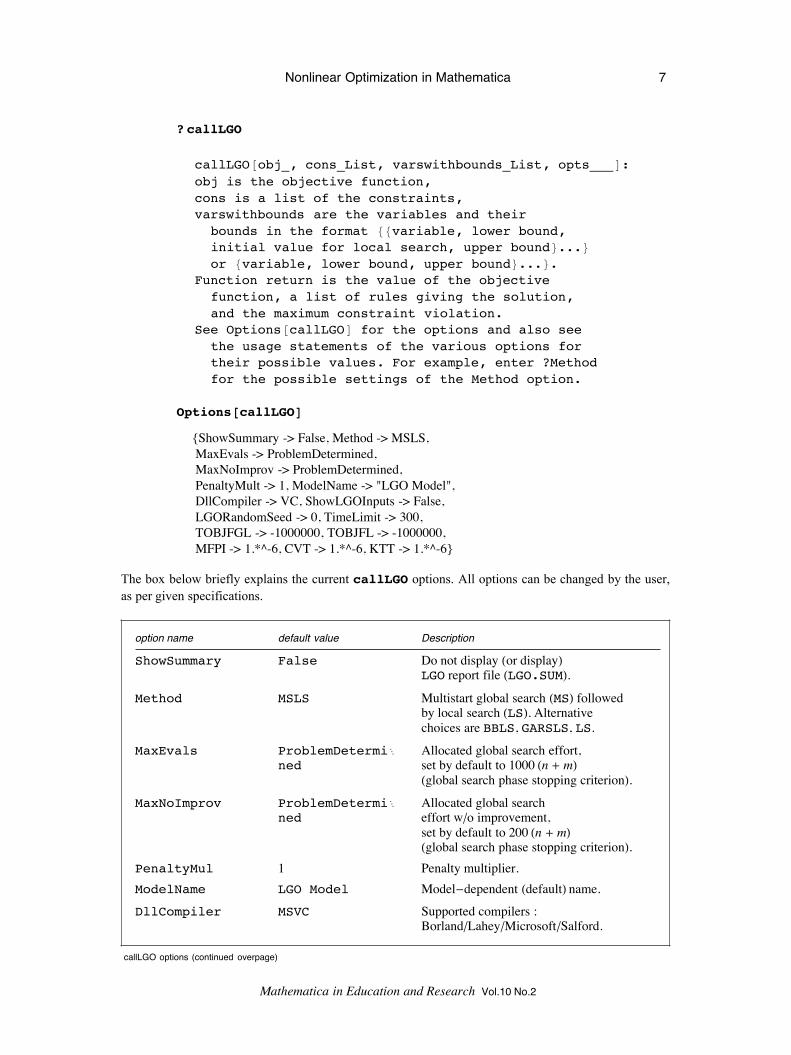
? callLGO

callLGO@obj_, cons_List, varswithbounds_List, opts___D:obj is the objective function,cons is a list of the constraints,varswithbounds are the variables and their

bounds in the format 88variable, lower bound,initial value for local search, upper bound<...<or 8variable, lower bound, upper bound<...<.

Function return is the value of the objectivefunction, a list of rules giving the solution,and the maximum constraint violation.

See Options@callLGOD for the options and also seethe usage statements of the various options fortheir possible values. For example, enter ?Methodfor the possible settings of the Method option.

Options@callLGOD{ShowSummary -> False, Method -> MSLS, MaxEvals -> ProblemDetermined, MaxNoImprov -> ProblemDetermined, PenaltyMult -> 1, ModelName -> "LGO Model", DllCompiler -> VC, ShowLGOInputs -> False, LGORandomSeed -> 0, TimeLimit -> 300, TOBJFGL -> -1000000, TOBJFL -> -1000000, MFPI -> 1.*^-6, CVT -> 1.*^-6, KTT -> 1.*^-6}

The box below briefly explains the current callLGO options. All options can be changed by the user,as per given specifications.

option name default value Description

ShowSummary False Do not display Hor displayLLGO report file HLGO.SUML.

Method MSLS Multistart global search HMSL followedby local search HLSL. Alternativechoices are BBLS, GARSLS, LS.

MaxEvals ProblemDetermiÖned

Allocated global search effort,set by default to 1000 Hn + mLHglobal search phase stopping criterionL.

MaxNoImprov ProblemDetermiÖned

Allocated global searcheffort wêo improvement,set by default to 200 Hn + mLHglobal search phase stopping criterionL.

PenaltyMul 1 Penalty multiplier.ModelName LGO Model Model-dependent HdefaultL name.DllCompiler MSVC Supported compilers :

BorlandêLaheyêMicrosoftêSalford.

callLGO options (continued overpage)



option name default value Description

ShowLGOInputs False Do not display Hor displayLthe generated LGO input files.

LGORandomSeed 0 Set to generate randomized search points.TimeLimit 300 Maximal allowed runtime Hin secondsLHglobal search phase stopping criterionL.TOBJFGL -1000000 Target objective function

value in global search phaseHglobal search phase stopping criterionL.TOBJFL -1000000 Target objective function value in local

search phase Hstopping criterionL.MFPI 10-6 Merit function precision

improvement toleranceHlocal search phase stopping criterionL.CVT 10-6 Accepted constraint violation toleranceHlocal search phase stopping criterionL.KTT 10-6 Kuhn-Tucker condition toleranceHlocal search phase stopping criterionL.

callLGO options

5. Circle packing problems

5.1 Introductory notes

A circle packing is a non-overlapping arrangement of circles inside a given set in 2 . This generalframework specifically includes the frequently studied case when all circles have the same (a prioriunknown, optimized) radius, and the circles are packed into the unit square or the unit circle. In thissection, illustrative numerical results are presented for these two special cases, as well as for the moregeneral case of packing non-uniform (in principle, arbitrary) size circles into an optimized circle.

Let us remark first that, in general, packings lead to difficult GO problems that can not be handled byclassical numerical approaches. Even the much simpler cases of packing identical size circles into asquare or into a circle are solved only for a few instances (up to a few tens of circles), to analytical orproven numerical optimality. This is in spite of the significant effort spent on variants of this problemby mathematical institutes and enthusiastic hobbyists for decades. From the massive packing literature,we refer here only to Melissen’s thesis [39] that provides extensive further pointers, and to the topicalwebsite of Specht [40] that cites best known results and related references.

Let us also emphasize that we will not exploit any prior structural considerations and heuristic initialarrangements that could help (significantly) in the optimization, since we wish to illustrate the generalsolver capabilities of MathOptimizer Professional. Although the case of packing uniform size circles isoften studied, the optimization approach advocated here can be directly brought to the more difficultcase of non-uniform size circle packings, as well as to other similar problems. To our best knowledge,the case of non-uniform circle packings, as introduced here, has not been investigated by other research-ers in optimization.

A Google web search with keywords ‘packing problems’ leads to hundreds of thousands of hits: manyof these hits indicate also the practical relevance of the subject. Uniform circle packings are closelyrelated to various models arising in numerical analysis, experimental design, computational physicsand chemistry, and in medical studies. The non-uniform circle packing model, and more general objectpackings, have practical applications e.g. in ergonomic design, dashboard design [41] or in actual(physical) packings [42].

We shall consider k circles with arbitrary radii rHiL > 0, for i = 1, …, k. Equal size circles can beconsidered as a special case of the general modeling framework presented below. We shall assume thatthe centers of the circles have coordinates xHiL and yHiL for i = 1, …, k: these are decision variables tobe determined. In addition, in the cases with identical circles, we will optimize their radius; in thegeneral circle packing case, we will optimize the radius of the circumscribing circle.



A circle packing is a non-overlapping arrangement of circles inside a given set in 2 . This generalframework specifically includes the frequently studied case when all circles have the same (a prioriunknown, optimized) radius, and the circles are packed into the unit square or the unit circle. In thissection, illustrative numerical results are presented for these two special cases, as well as for the moregeneral case of packing non-uniform (in principle, arbitrary) size circles into an optimized circle.

Let us remark first that, in general, packings lead to difficult GO problems that can not be handled byclassical numerical approaches. Even the much simpler cases of packing identical size circles into asquare or into a circle are solved only for a few instances (up to a few tens of circles), to analytical orproven numerical optimality. This is in spite of the significant effort spent on variants of this problemby mathematical institutes and enthusiastic hobbyists for decades. From the massive packing literature,we refer here only to Melissen’s thesis [39] that provides extensive further pointers, and to the topicalwebsite of Specht [40] that cites best known results and related references.

Let us also emphasize that we will not exploit any prior structural considerations and heuristic initialarrangements that could help (significantly) in the optimization, since we wish to illustrate the generalsolver capabilities of MathOptimizer Professional. Although the case of packing uniform size circles isoften studied, the optimization approach advocated here can be directly brought to the more difficultcase of non-uniform size circle packings, as well as to other similar problems. To our best knowledge,the case of non-uniform circle packings, as introduced here, has not been investigated by other research-ers in optimization.

A Google web search with keywords ‘packing problems’ leads to hundreds of thousands of hits: manyof these hits indicate also the practical relevance of the subject. Uniform circle packings are closelyrelated to various models arising in numerical analysis, experimental design, computational physicsand chemistry, and in medical studies. The non-uniform circle packing model, and more general objectpackings, have practical applications e.g. in ergonomic design, dashboard design [41] or in actual(physical) packings [42].

We shall consider k circles with arbitrary radii rHiL > 0, for i = 1, …, k. Equal size circles can beconsidered as a special case of the general modeling framework presented below. We shall assume thatthe centers of the circles have coordinates xHiL and yHiL for i = 1, …, k: these are decision variables tobe determined. In addition, in the cases with identical circles, we will optimize their radius; in thegeneral circle packing case, we will optimize the radius of the circumscribing circle.

5.2 Non-overlapping circle arrangements

The condition that circles i and j must not overlap is equivalent to requiring that the sum of their radiican not be greater than the Euclidean distance between their centers:

(3) rHiL + rH jL §"########################################################HxHiL - xH jLL2 + HyHiL - yH jLL2 for i, j = 1, …, k and i < j

Next we shall summarize the objective function and constraints for the three types of problems consid-ered here. In addition to the ‘no-overlap’ constraints formulated above, a second set of constraintspostulate that the circles are inside the enclosing circle or square. The latter constraints are also derivedfrom simple geometrical considerations.

5.3 Packing equal size circles in the unit square

We shall consider first the case of packing identical circles in the unit square that is, by assumption,centered around the origin. Then the optimization model is formulated as follows:

(4) max r

(5) À xHiL À +r §1ÅÅÅÅÅ2

for i = 1, …, k

(6) À yHiL À +r §1ÅÅÅÅÅ2

for i = 1, …, k

(7) 2r §"########################################################HxHiL - xH jLL2 + HyHiL - yH jLL2 for i, j = 1, …, k and i < j

Observe that we have 2k nonlinear convex constraints, and kHk - 1L ê2 non-convex constraints (sincethe norm function itself is convex). A Mathematica function which implements this model, returningthe objective function, constraints, and variables with bounds is as follows:

In[1]:= circumscribecircles@k_IntegerD :=

ModuleAH* local variables in the module *L8cons, cons1, cons2, cons3, vars, lb, ub, soln, r<,



In[1]:=

H* the set of no-overlap constraints *Lcons1 =

Flatten ATableA "######################################################################Hx@iD - x@jDL2 + Hy@iD - y@jDL2 ¥ 2 r,8i, k - 1<, 8j, i + 1, k<EE;H* the constraint set which keeps the circles inside - 1ÄÄÄÄÄ2

£

x < 1ÄÄÄÄÄ2

*Lcons2 = TableAr + Abs@x@iDD §

1ÅÅÅÅ2, 8i, k<E;H* the constraint set which keeps the circles inside - 1ÄÄÄÄÄ

2£

y < 1ÄÄÄÄÄ2

*Lcons3 = TableAr + Abs@y@iDD §

1ÅÅÅÅ2, 8i, k<E;H* the variables are the circle center coordinates

and the radius of the identical circles *Lvars = Join@Flatten@Table@8x@iD, y@iD<, 8i, k<DD, 8r<D;H* join all the constraints *Lcons = Join@cons1, cons2, cons3D;H* lower and upper bounds on the variables *Llb = Join@Table@-1, 82 * k<D, 80<D;ub = Join@Table@1, 82 * k<D, 81. ê Sqrt@p kD<D;H* the objective function Hnegative since we want

to maximize r , constraints and variables *L8-r, cons, Transpose@8vars, lb, ub<D<E5.4 Packing equal size circles in the unit circle

Next, we consider the case of packing identical circles in the unit circle with its center at the origin.Then the optimization model is:

(8) max r

(9) "########################xHiL2 + yHiL2 + r § 1 for i = 1, …, k

(10) 2r §"########################################################HxHiL - xH jLL2 + HyHiL - yH jLL2 for i, j = 1, …, k and i < j

Consequently, now we have k convex nonlinear constraints, in addition to the kHk - 1L ê2 non-convexconstraints. The Mathematica model is very similar to the model for the unit square.


ModuleA8cons, cons1, cons2, vars, lb, ub, soln, r<,cons1 =



In[2]:=

Flatten ATableA "######################################################################Hx@iD - x@jDL2 + Hy@iD - y@jDL2 ¥ 2 r,8i, k - 1<, 8j, i + 1, k<EE;H* the constraint which keeps the circlesinside the circumscribing circle *L

cons2 = TableAr +"###############################

x@iD2 + y@iD2 § 1, 8i, k<E;vars = Join@Flatten@Table@8x@iD, y@iD<, 8i, k<DD, 8r<D;cons = Join@cons1, cons2D;lb = Join@Table@-1, 82 * k<D, 80<D;ub = Join@Table@1, 82 * k<D, 81. ê Sqrt@kD<D;8-r, cons, Transpose@8vars, lb, ub<D<E

5.5 Packing circles of various size into the smallest circumscribing circle

In this case, we have to find the circle of optimized radius, with its center at the origin, that contains allthe given circles in a non-overlapping arrangement. The corresponding optimization model is:

(11) min r

(12) "########################xHiL2 + yHiL2 + rHiL § r for i = 1, …, k

(13) rHiL + rH jL § "########################################################HxHiL - xH jLL2 + HyHiL - yH jLL2 for i, j = 1, …, k and i < j

Similarly to the model above, we have k convex (nonlinear) constraints and kHk - 1L ê 2 non-convexconstraints.

The above model formulations imply that the complexity of all three packing models increases rapidly,as k increases. The Mathematica function is more complex than the previous ones due to the differentsizes of the circles.


ModuleA8cons, cons1, cons2, vars, lb, ub, soln, rcirc<,H* generate the radii of the k circles *LDo@r@iD = i-1ê2, 8i, k<D;cons1 = Flatten A

TableAr@iD + r@jD §"######################################################################Hx@iD - x@jDL2 + Hy@iD - y@jDL2 ,8i, k - 1<, 8j, i + 1, k<EE;H* constrain the n circles to be inside

the circumscribing circle *Lcons2 = TableArcirc - r@iD ¥

"###############################x@iD2 + y@iD2 , 8i, k<E;



In[3]:=

vars =Join@Flatten@Table@8x@iD, y@iD<, 8i, k<DD, 8rcirc<D;

cons = Join@cons1, cons2D;lb = Join@[email protected], 82 * k<D, 81<D;ub = Join@[email protected], 82 * k<D, 83<D;8rcirc, cons, Transpose@8vars, lb, ub<D<E

5.6 Illustrative numerical results

In this section we present some numerical results for the three packing models defined in the previoussection. These results have been calculated using MOP in conjunction with the Salford FORTRAN FTN95 compiler. The computer used has a 3.2 GHz Pentium Pro processor and it is running under Win-dows XP. Mathematica graphics primitives were used in constructing the results shown.

In the case of packing 20 identical size (optimized) circles in the unit square we have obtained theradius r ~ 0.1113823475. This value agrees to at least 10-10 absolute precision with the best knownvalue 0.111382347512 posted at www.packomania.com. Figure 1 displays the arrangement found. Asper our related notes, this 20 circle model has 2k + 1 = 41 decision variables, 2k = 40 nonlinear convexconstraints, and kHk - 1L ê2 = 190 non-convex constraints. The corresponding MOP runtime is approxi-mately 18 seconds.

Fig. 1 Optimized configuration of 20 identical size circles in the unit square.



In the next example, for packing 20 identical size circles in the unit circle we have obtained the(optimized) radius r ~ 0.1952240110. Again, this value agrees to at least 10-10 absolute precision withthe best known value 0.195 224 011 018 748 878 291 305 694 833 posted at www.packomania.com.Figure 2 displays the arrangement found. This 20 circle model has 2k + 1 = 41 decision variables,k = 20 nonlinear convex constraints, and kHk - 1L ê2 = 190 non-convex constraints. The correspondingMOP runtime is approximately 43 seconds.

Fig. 2 Optimized configuration of 20 identical size circles in the unit circle.

In the last numerical example shown here, we have been packing circles of size i-1ê2 for i = 1, …, kinto a circumscribing circle that is centered at the origin, and minimized its radius. Note that the total

area of the packed circles is slowly divergent as k goes to infinity (since their total area is p‚i=1

k

1 ê i):

therefore the optimized radius also goes to infinity as k grows. Figure 3 shows the configuration found:the radius of the circumscribing circle is r ~2.1246798149. The MOP runtime is 47 seconds: this isonly about 10 percent higher than for solving the special case of uniform size circles (for the samenumber of circles).



Fig. 3 Optimized configuration of 20 non-uniform size circles in a circle.

Let us point out again that structural considerations and heuristic initial arrangements have not beenused to generate these results. This fact illustrates the core (default) numerical capabilities of MathOpti-mizer Professional, at least for the examples presented in this paper. So far, we solved packing modelsfor up to k = 40 circles. The longest runs take 3 to 4 hours on P4 processor based computers [43]. If wewished to solve larger model instances, then some more advanced modeling (and perhaps also heuris-tic) considerations should also be exploited, to speed up the solution procedure.

From an optimization standpoint, packing different size circles into a circumscribing circle is a muchmore complex problem than packing equal size circles since there are many local minima close invalue to the global minimum. Many of these local minima can be regarded as arising from interchang-ing two circles in the global solution and then suitably ‘readjusting’ the other circles. Such inter-changes have no effect on the solution when packing equal size circles. Therefore packing unequal sizecircles can be used to test global optimizers for the class of problems that have a large number of localminima close in value to the global minimum: such models occur frequently e.g. in computationalphysics and chemistry.

The results of such a test are shown in Figures 4 and 5.The time required and the objective functionvalues obtained for 10 sequentially performed optimizations (using different random seeds) are shownfor packing 3 to 10 circles, for both MathOptimizer Professional and the built-in Mathematica functionNMinimize. The Multistart method was used for MathOptimizer Professional and the DifferÖential Evolution method was used for NMinimize as these methods give the best results forthis class of problems for the two optimizers. In both figures, MathOptimizer Professional performanceis shown by black (darker) dots, and NMinimize performance is shown by red (lighter) dots.



3 4 5 6 7 8 9 10Number of Circles

5

10

50

100

500

t

Fig. 4 Timing comparison (seconds) between MathOptimizer Professional and NMinimize for unequal circle packing. The results are based on 10 sequentially performed optimizations, using different random seeds.

3 4 5 6 7 8 9 10Number of Circles

1.75

1.8

1.85

1.9

1.95

2

2.05

r

Fig. 5 Plot of circumscribing radius, r, versus number of circles shows the objective function value comparison between MathOptimizer Professional and NMinimize for unequal circle packing. The results are based on 10 sequentially performed optimizations, using different random seeds.

The results summarized by the figures show that MathOptimizer Professional ran faster and gave betterresults than NMinimize in the circle packing tests. It should be noted, however, that for simpler andsmall-size optimization problems with a small number of local minima, NMinimize often returns thesame result in less time than MathOptimizer Professional. This is due to the ‘overhead’ incurred inMathOptimizer Professional in compiling the model file, as well as to the MathLink based communica-tion between the Mathematica notebook and LGO. (The LGO solver suite runs faster than the total timespent on using the callLGO function.)

We also note that MathOptimizer Professional perfomance compares favorably also to that of severalother global optimization packages that we have applied to solve non-uniform circle packing models.More detailed comparative results will be presented elsewhere.



6. Concluding Remarks

In this article, we discuss the potentials of Mathematica in OR/MS studies, with a special relevance innonlinear systems modeling and optimization. Following the introduction of the general global optimiza-tion model, we present MathOptimizer Professional with an external link to the LGO solver engine.

The usage of MOP is illustrated by solving non-trivial numerical examples. The circle packing modelsdiscussed can serve as test models to benchmark global optimization software. Although all numericaltest reports depend also on solver parameterizations and other circumstances, the examples presentedindicate the capabilities and potentials of MathOptimizer Professional. In this context, we also refer toanother recent computational study [44] that compares the performance of the GAMS/LGO implementa-tion to state-of-art local solvers. This evaluation, that also shows the comparative merits of the LGOsolver suite, has been done in a fully automated fashion using the GAMS model libraries. Therefore itcan be considered as reasonably objective, although the collection of available models and othercircumstances always carry elements of arbitrariness and subjectivity. (The details of this performanceanalysis, including the paper mentioned, are directly available from http://www.gams.com/solvers/solvers.htm#LGO. )

For over a decade, LGO has been applied in a large variety of research and professional contexts: forexamples and case studies see references [27, 29, 45-48]. We expect an essentially similar performancefrom MathOptimizer Professional that enables the solution of sizeable, sophisticated Mathematicamodels, with an efficiency comparable to that of compiler-based nonlinear solvers.

Acknowledgements

We wish to thank Mark Sofroniou (Wolfram Research) for his permission to use, and to customize, theFormat.m package in our MOP software development work. We received useful comments andadvice from two anonymous referees, as well as from Daniel Lichtblau (Wolfram Research) andIgnacio Castillo (University of Alberta).

JDP’s research in recent years has been partially supported by grants received from the NationalResearch Council of Canada (NRC IRAP Project No. 362093) and from the Hungarian ScientificResearch Fund (OTKA Grant No. T 034350). JDP also wishes to acknowledge the support receivedfrom Wolfram Research over the years, in forms of a visiting scholarship, books, software, and profes-sional advice.

References

[1] S. Wolfram (2003) The Mathematica Book. (5th Edition.) Wolfram Media, Champaign, IL, andCambridge University Press, Cambridge, UK.

[2] Mathematica Information Center http://library.wolfram.com/.

[3] P.C. Bell (1999) Management Science / Operations Research – A Strategic Perspective. South-West-ern College Publishing / Thomson Learning, Cincinnati, OH.

[4] D. Bertsimas and R.M. Freund, R.M. (2000) Data, Models, and Decisions. South-Western CollegePublishing / Thomson Learning, Cincinnati, OH.

[5] M.A. Bhatti (2000) Practical Optimization Methods with Mathematica Applications. Springer, NewYork, NY.

[6] M.W. Carter and C.C. Price (2001) Operations Research: A Practical Introduction. CRC Press,Boca Raton, FL.



[7] U. Diwekar (2003) Introduction to Applied Optimization. Kluwer Academic Publishers, Dordrecht.

[8] T.F. Edgar, D.M. Himmelblau and L.S. Lasdon (2001) Optimization of Chemical Processes. (2ndEdition.) McGraw-Hill, NY.

[9] F.S. Hillier and G.J. Lieberman (2005) Introduction to Operations Research. (8th Edition.)McGraw-Hill, New York, NY.

[10] W.L. Winston and S.C. Albright (2001) Practical Management Science. (2nd Edition.) Duxbury /Thomson Learning, Pacific Grove, CA.

[11] INFORMS www.informs.org.

[12] R. Aris (1999) Mathematical Modeling: A Chemical Engineer’s Perspective. Academic Press, SanDiego, CA.

[13] T.B. Bahder (1995) Mathematica for Scientists and Engineers. Addison-Wesley, Reading, MA.

[14] R. Gass (1998) Mathematica for Scientists and Engineers: Using Mathematica to do Science.Prentice Hall, Englewood Cliffs, NJ.

[15] N.A. Gershenfeld (1999) The Nature of Mathematical Modeling. Cambridge University Press,Cambridge, UK.

[16] J.D. Murray (1983) Mathematical Biology. Springer, Berlin.

[17] A. Neumaier (1997) Molecular modeling of proteins and mathematical prediction of proteinstructure. SIAM Review 39, 407-460.

[18] P.Y. Papalambros and D.J. Wilde (2000) Principles of Optimal Design. Cambridge UniversityPress, Cambridge, UK.

[19] K. Schittkowski (2002) Numerical Data Fitting in Dynamical Systems. Kluwer Academic Publish-ers, Dordrecht.

[20] M. Schroeder (1991) Fractals, Chaos, Power Laws. Freeman & Co., New York.

[21] C.A. Floudas and P.M. Pardalos, Eds. (2000) Optimization in Computational Chemistry andMolecular Biology: Local and Global Approaches. Kluwer Academic Publishers, Dordrecht.

[22] C.A. Floudas, P.M. Pardalos, C. Adjiman, W.R. Esposito, Z.H. Gumus, S.T. Harding, J.L.Klepeis, C.A. Meyer and C.A. Schweiger (1999) Handbook of Test Problems in Local and GlobalOptimization. Kluwer Academic Publishers, Dordrecht.

[23] I.E. Grossmann, Ed. (1996) Global Optimization in Engineering Design. Kluwer AcademicPublishers, Dordrecht.

[24] F.J. Kampas and J.D. Pintér (2005) Advanced Optimization: Scientific, Engineering, and Eco-nomic Applications with Mathematica Examples. Elsevier, Amsterdam. (Forthcoming.)

[25] P.M. Pardalos, D. Shalloway and G. Xue (1996) Global Minimization of Nonconvex EnergyFunctions: Molecular Conformation and Protein Folding. DIMACS Series, Vol. 23, American Mathe-matical Society, Providence, RI.

[26] J.D. Pintér (1996) Global Optimization in Action (Continuous and Lipschitz Optimization: Algo-rithms, Implementations and Applications). Kluwer Academic Publishers, Dordrecht.

[27] J.D. Pintér ( 2001) Computational Global Optimization in Nonlinear Systems: An InteractiveTutorial. Lionheart Publishing, Atlanta, GA.

[28] J.D. Pintér (2002) Global optimization: software, test problems, and applications. Chapter 15 (pp.515-569) in: Pardalos and Romeijn, Eds., Handbook of Global Optimization, Vol. 2. Kluwer AcademicPublishers, Dordrecht.

[29] J.D. Pintér (2005) Applied Nonlinear Optimization in Modeling Environments. CRC Press, BocaRaton, FL, 2005. (Forthcoming.)



[30] M. Tawarmalani and N.V. Sahinidis (2002) Convexification and Global Optimization in Continu-ous and Mixed-Integer Nonlinear Programming. Kluwer Academic Publishers, Dordrecht.

[31] Z.B. Zabinsky (2003) Stochastic Adaptive Search for Global Optimization. Kluwer AcademicPublishers, Dordrecht.

[32] A. Neumaier (2003) Complete search in continuous optimization and constraint satisfaction. In:Iserles, A., Ed. Acta Numerica 2004. Cambridge University Press, Cambridge, UK.

[33] R. Horst, R. and P.M. Pardalos, Eds. (1995) Handbook of Global Optimization, Vol. 1. KluwerAcademic Publishers, Dordrecht.

[34] P.M. Pardalos and H.E. Romeijn, Eds. (2002) Handbook of Global Optimization, Vol. 2. KluwerAcademic Publishers, Dordrecht.

[35] J.D. Pintér (2005) LGO – An Integrated Model Development and Solver Environment for Continu-ous Global Optimization. User Guide. (Current Edition.) Pintér Consulting Services, Inc., Halifax, NS,Canada.

[36] H.P. Benson and E. Sun (2000) LGO – Versatile tool for global optimization. ORMS Today 27 (5)52-55. Internet version is available at http://www.lionhrtpub.com/orms/orms-10-00/swr.html.

[37] C.G.E. Boender and H.E. Romeijn (1995) Stochastic methods. Chapter 14 (pp. 829-869) in: Horstand Pardalos, Eds. Handbook of Global Optimization, Vol. 1. Kluwer Academic Publishers, Dordrecht.

[38] J.D. Pintér and F.J. Kampas (2003) MathOptimizer Professional – An Advanced Modeling andOptimization System for Mathematica Users with an External Solver Link. User Guide. Pintér Consult-ing Services, Inc., Halifax, NS, Canada.

[39] J.B.M. Melissen (1997) Packing and Covering with Circles. Ph.D. Dissertation, UniversiteitUtrecht, The Netherlands.

[40] E. Specht http://www.packomania.com/.

[41] M.D. Riskin, K.C. Bessette and I. Castillo (2003) A logarithmic barrier approach to solving thedashboard planning problem. INFOR 41, 245-257.

[42] Y.Y. Stoyan, G. Yaskov and G. Scheithauer (2003) Packing of various solid spheres into aparalellepiped. CEJOR 11, 389-407.

[43] F.J. Kampas and J.D. Pintér (2004) Generalized circle packings: model formulations and numeri-cal results. Proceedings of the 6th International Mathematica Symposium (Banff, AB, Canada August1-6, 2004).

[44] J.D. Pintér (2003) GAMS/LGO nonlinear solver suite: key features, usage, and numerical perfor-mance. (Submitted for publication.) Available from http://www.gams.com/solvers/solvers.htm#LGO.

[45] J.D. Pintér (2001) Globally optimized spherical point arrangements: model variants and illustra-tive results. Annals of Operations Research 104, 213-230.

[46] F.J. Kampas and J.D. Pintér (2005) Configuration analysis and design by using optimization toolsin Mathematica. The Mathematica Journal (To appear).

[47] G. Isenor, J.D. Pintér and M. Cada (2003) A global optimization approach to laser design. Optimi-zation and Engineering 4, 177-196.

[48] J. Tervo, P. Kolmonen, T. Lyyra-Laitinen, J.D. Pintér and T. Lahtinen (2003) An optimization-based approach to the multiple static delivery technique in radiation therapy. Annals of OperationsResearch 119, 205-227.



Documents

Nonlinear Optimization in Mathematica with MathOptimizer ... · Nonlinear Optimization in Mathematica with MathOptimizer Professional János D. Pintér1 and Frank J. Kampas2 1. Pintér