Nonlinear Optimization Benny Yakir

These notes are based on help files of MATLAB’soptimization toolbox and on the book

Linear and Nonlinear Programing by D.G. Luenberger.No originality is claimed.

**************************************************** ****************************************************

Contents

1 The General Optimization Problem 3

2 Basic properties of solutions and algorithms 52.1 Necessary conditions for a local optimum . . . . . . . . . . . 52.2 Global convergence of decent algorithms . . . . . . . . . . . 72.3 Homework . . . . . . . . . . . . . . . . . . . . . . . . . . . . . 8

3 Basic MATLAB 103.1 Files and Directories in UNIX . . . . . . . . . . . . . . . . . . 103.2 Other UNIX Commands . . . . . . . . . . . . . . . . . . . . . 103.3 Starting and quitting MATLAB . . . . . . . . . . . . . . . . . 103.4 Matrices . . . . . . . . . . . . . . . . . . . . . . . . . . . . . . 113.5 Graphics . . . . . . . . . . . . . . . . . . . . . . . . . . . . . . 133.6 Scripts and functions . . . . . . . . . . . . . . . . . . . . . . . 133.7 Files . . . . . . . . . . . . . . . . . . . . . . . . . . . . . . . . 143.8 Homework . . . . . . . . . . . . . . . . . . . . . . . . . . . . . 15

4 Basic descent methods 164.1 Fibonacci and Golden Section Search . . . . . . . . . . . . . 164.2 Newton’s method . . . . . . . . . . . . . . . . . . . . . . . . 164.3 Applying line-search methods . . . . . . . . . . . . . . . . . . 174.4 Quadratic interpolation . . . . . . . . . . . . . . . . . . . . . 184.5 Cubic fit . . . . . . . . . . . . . . . . . . . . . . . . . . . . . . 194.6 Homework . . . . . . . . . . . . . . . . . . . . . . . . . . . . . 19

1

5 The method of steepest decent 215.1 The quadratic case . . . . . . . . . . . . . . . . . . . . . . . . 215.2 Applying the method in Matlab . . . . . . . . . . . . . . . . . 225.3 Homework . . . . . . . . . . . . . . . . . . . . . . . . . . . . . 25

6 Newton and quasi-Newton methods 266.1 Newton’s method . . . . . . . . . . . . . . . . . . . . . . . . 266.2 Extensions . . . . . . . . . . . . . . . . . . . . . . . . . . . . . 266.3 The Davidon-Fletcher-Powell (DFP) method . . . . . . . . . 276.4 The Broyden-Flecher-Goldfarb-Shanno (BFGS) method . . . 286.5 The function fminunc . . . . . . . . . . . . . . . . . . . . . . 296.6 Examples . . . . . . . . . . . . . . . . . . . . . . . . . . . . . 306.7 Homework . . . . . . . . . . . . . . . . . . . . . . . . . . . . . 316.8 Project 1 . . . . . . . . . . . . . . . . . . . . . . . . . . . . . 31

7 Constrained Minimization Conditions 337.1 Necessary conditions (equality constraints) . . . . . . . . . . 337.2 Examples . . . . . . . . . . . . . . . . . . . . . . . . . . . . . 347.3 Necessary conditions (inequality constraints) . . . . . . . . . 367.4 Sufficient conditions . . . . . . . . . . . . . . . . . . . . . . . 377.5 Sensitivity . . . . . . . . . . . . . . . . . . . . . . . . . . . . . 387.6 Homework . . . . . . . . . . . . . . . . . . . . . . . . . . . . . 39

8 Lagrange methods 408.1 Quadratic programming . . . . . . . . . . . . . . . . . . . . . 40

8.1.1 Equality constraints . . . . . . . . . . . . . . . . . . . 408.1.2 Inequality constraints . . . . . . . . . . . . . . . . . . 41

8.2 Sequential Quadratic Programming . . . . . . . . . . . . . . 428.3 Newton’s Method . . . . . . . . . . . . . . . . . . . . . . . . 428.4 Structured Methods . . . . . . . . . . . . . . . . . . . . . . . 428.5 Merit function . . . . . . . . . . . . . . . . . . . . . . . . . . 438.6 Enlargement of the feasible region . . . . . . . . . . . . . . . 448.7 The Han–Powell method . . . . . . . . . . . . . . . . . . . . 458.8 Constrained minimization in Matlab . . . . . . . . . . . . . . 458.9 Constrained minimization in Matlab (using the function fmincon 468.10 Homework . . . . . . . . . . . . . . . . . . . . . . . . . . . . . 49

9 Large scale problems 519.1 Basic issues . . . . . . . . . . . . . . . . . . . . . . . . . . . . 519.2 Minimization with no constraints. Hassien provided . . . . . 52

2

9.3 Minimization with no constraints. Hassien not provided . . . 549.4 Minimization with constraints. . . . . . . . . . . . . . . . . . 559.5 Project 2 . . . . . . . . . . . . . . . . . . . . . . . . . . . . . 56

10 Penalty and Barrier Methods 5710.1 Penalty method . . . . . . . . . . . . . . . . . . . . . . . . . . 5710.2 Barrier method . . . . . . . . . . . . . . . . . . . . . . . . . . 59

3

1 The General Optimization Problem

The general optimization problem has the form:

minx∈Rd

f(x)

subject to:

gi(x) = 0 i = 1, . . . ,me

gi(x) ≤ 0 i = me + 1, . . . ,mxl ≤ x ≤ xu

In particular, if m = 0, the problem is called an unconstrained optimizationproblem. In this course we intend to introduce and investigate algorithms forsolving this problem. We will concentrate, in general, in algorithms whichare used by the Optimization toolbox of MATLAB.

We intend to cover the following sections:

Basic properties of solutions and algorithms: In this section we con-sider general conditions for the existence of a solution. We also definethe terms algorithm, iterative algorithm and descent algorithm.

Basic MATLAB: Here we introduce the basic features and structure ofthe MATLAB system.

Line descent methods: Here we deal with algorithms for finding the min-imum in the case where d = 1. These algorithms are the basic buildingblocks when solving more complex optimization problems.

The method of steepest descent: In each iteration, a line search is per-formed in the direction of the steepest descent.

Newton and Quasi-Newton methods: In the Newton method the func-tion is approximated (locally) by a quadratic form. The direction ofthe search is chosen based on this form. Quasi-Newton methods re-place the Hassian with terms which are easier to evaluate.

Conditions in constraint minimization: The conditions that were con-sidered in section 1 for unconstrained problems are modified in order todeal with constraint. The Lagrange multipliers and the Kuhn-Tuckerconditions are described.

4

Lagrange methods: These methods are based on the Lagrange first-orderconditions of a solution. The method is applied for quadratic pro-graming.

Sequential Quadratic Programming: At each iteration the function andLagrange multipliers are approximated by a quadratic programingproblem.

Penalty and barrier methods: A sequence of unconstrained minimiza-tion problem is solved. The solution to these problems converge tothe solution of the original problem.

Time permitting, we would also like to deal with other optimizationproblems. Examples include: the EM algorithm, discrete optimization usingdynamic programing, stochastic approximation.

5

2 Basic properties of solutions and algorithms

2.1 Necessary conditions for a local optimum

Assume that the function f is defined over Ω ⊂ Rd.Definition: A point x∗ ∈ Ω is said to be a relative minimum point or a

local minimum point of f if there is an ε > 0 such that f(x∗) ≤ f(x)for all x such that ‖x−x∗‖ < ε. If the inequality is strict for all x 6= x∗

then x∗ is said to be a strict relative minimum point.

Definition: A point x∗ ∈ Ω is said to be a global minimum point of f iff(x∗) ≤ f(x) for all x ∈ Ω. If the inequality is strict for all x 6= x∗

then x∗ is said to be a strict global minimum point.

In practice, the algorithms we will consider in the better part of thiscourse converge to a local minimum. We may indicate in some cases howthe global minimum can be attained.Definition: Given x ∈ Ω, a vector d is a feasible direction at x if there

exists an α > 0 such that x + αd ∈ Ω for all 0 ≤ α ≤ α.

Theorem 2.1 (First-order necessary conditions.) Let f ∈ C1. If x∗

is a relative minimum, then for any vector d which is feasible at x∗, wehave f(x∗)′d ≥ 0. (f(x∗) is the vector of partial derivatives of f at x∗.)

Corollary 2.1 If x∗ is a relative minimum and if x∗ ∈ Ω0 then f(x∗) = 0.

Example 2.1 Consider the function f(x, y) = x2 − xy + y2 − 3y, withΩ = R2. From the first order conditions we get that x∗ = 1 and y∗ = 2.This is a global minimum.

Example 2.2 Consider the function f(x, y) = x2 − x + y + xy, with Ω =(R+)2. The global minimum is at x∗ = 0.5 and y∗ = 0. At this point,f(0.5, 0) = (0, 3/2)′.

6

Example 2.3 Let the production function be f(x1, . . . , xd), where xi are theinputs. The unit price of the produced commodity is q and the unit price ofthe ith input is pi. The producer wants to maximize

qf(x1, . . . , xd)− p1x1 − · · · − pdxd.

The first order conditions can be interpreted as stating that the marginalvalue increase must be equal to pi.

Example 2.4 We observe g(x) at the points x1, . . . , xm. We want to ap-proximate the function with a polynomial of the form h(x) =

∑d−1j=0 ajx

j, ford < m. Consider the minimization problem

mina∈Rd

m∑k=1

[g(xk)− h(xk)]2 = mina∈Rd

m∑k=1

[g(xk)−∑d−1j=0 ajx

jk]

2 = mina∈Rd f(a).

Let qij =∑mk=1(xk)i+j, bj =

∑mk=1 g(xk)(xk)j and c =

∑mk=1 g(xk)2. Then

f(a) = a′Qa− 2b′a + c,

and the first order conditions are

Qa = b.

Second order conditions deal with functions with continuous second par-tial derivatives and uses the Hessian matrix f(x∗) of (mixed) partial deriva-tives.

Theorem 2.2 (Second-order necessary conditions.) Let f ∈ C2. Letx∗ be a relative minimum. For any vector d which is feasible at x∗, iff(x∗)′d = 0 then d′f(x∗)d ≥ 0.

Corollary 2.2 If x∗ is a relative minimum and if x∗ ∈ Ω0 then f(x∗)′d =0 and d′f(x∗)d ≥ 0 for all d.

Example 2.5 Consider the function f(x, y) = x2 − x2y + 2y2, with Ω =(R+)2. The first order conditions are

3x2 − 2xy = 0, −x2 + 4y = 0.

There are two solutions: (0, 0) and (6, 9). However, the second is not arelative minimum since the Hessian matrix

f(6, 9) =[

18 −12−12 4

]is not positive semi-definite.

7

Theorem 2.3 (Second-order sufficient conditions.) Let f ∈ C2. As-sume that x∗ ∈ Ω0. If f(x∗) = 0 and f(x∗) is positive definite then x∗ is astrict relative minimum.

2.2 Global convergence of decent algorithms

The algorithms we consider are iterative descent algorithms. By iterative wemean, roughly, that the algorithm generates a series of points, each pointbeing calculated on the basis of the points preceding it. By descent wemean that the sequence of values of some function, calculated at the pointsgenerated by the algorithm, is a monotone decreasing sequence.

Definition: An algorithm A is a mapping that assigns, to each point, asubset of the space.

Iterative algorithm: The specific sequence is constructed by choosing apoint in the subset and iterating the process. Thus algorithm generatesa series of points, and each point is calculated on the basis of the pointspreceding it.

Descent algorithm: As each new point is generated, the correspondingvalue of some function decreases in value. Specifically, there exists acontinuous function Z such that if A is the algorithm and Γ is thesolution set then

1. If x 6∈ Γ and y ∈ A(x), then Z(y) < Z(x).

2. If x ∈ Γ and y ∈ A(x), then Z(y) ≤ Z(x).

Definition: An algorithm is said to be globally convergent if, for any start-ing point, it generates a sequence that converges to a solution.

Definition: A point-to-set map A is said to be closed at x if

1. xk → x and

2. yk → y,yk ∈ A(xk), imply

3. y ∈ A(x).

The map A is closed if it is closed at each point of the space.

8

Example 2.6 Suppose for x ∈ R we define A(x) = [−x/2, x/2]. Startingat x0 = 100, each of the sequences

100, 50, 25, 12,−6,−2, 1, 1/2, . . .100,−40, 20,−5,−2, 1, 1/4, 1/8, . . .100, 10, 1/16, 1/100,−1/1000, 1/10000, . . .

might be generated from iterative application of the algorithm. The givenalgorithm is closed.

Example 2.7 If A is point-to-point and continuous them A is closed.

Theorem 2.4 If A is a decent iterative algorithm which is closed outsideof the solution set Γ and if the sequence of points is contained in a compactset then any converging subsequence converges to a solution.

2.3 Homework

1. To approximate the function g over the interval [0, 1] by a polynomial hof degree n (or less), we use the criterion

f(a) =∫ 1

0[g(x)− h(x)]2dx,

where a ∈ Rn+1 are the coefficients of h. Find the equations satisfied bythe optimal solution.

2.(a) Using first-order necessary conditions, find the minimum of the function

f(x, y, z) = 2x2 + xy + y2 + yz + z2 − 6x− 7y − 8z + 9.

(b) Verify the point is a relative minimum by checking the second-orderconditions.

3. In control problem one is interested in finding numbers u0, . . . , un thatminimize the objective function

J =n∑k=0

(x0 + u0 + · · ·+ uk−1)2 + u2k,

for a given x0. Find the equations that determine the first order condi-tions.

9

4. Define the point-to-set mapping on Rn by

A(x) = y : y′x ≤ b,

where b is a fixed constant. Is A closed?

10

3 Basic MATLAB

The name MATLAB stands for matrix laboratory. It is an interactive systemfor technical computing whose basic data element is an array that does notrequire dimensioning.

3.1 Files and Directories in UNIX

The home dir is ‘‘~’’, the current dir is ‘‘.’’ and one dir up is‘‘..’’.

mkdir dirname creates a directory dirname.cd path/dirname moves the working directory to dirname.ls lists the content of the working directory.less lists the content of the file filename.cp file1 file2 copies file1 into file2.cp file dir copies file into dir.rm file deletes file.

3.2 Other UNIX Commands

man command help on command.arrows move through commands typed in the past.tab tries to completes commands.Control-c kills a running job.emacs file & editing file with emacs.pico file editing file with pico.

3.3 Starting and quitting MATLAB

Starting on pluto: /applic/matlab.5.3/bin/matlab.Starting on shum: matlab.Quitting: Write quit.Set the display: setenv DISPLAY xterm:0Help: help function name,

helpwin,lookfor topic.

11

3.4 Matrices

MATLAB is case sensitive. Memory is allocated automatically.

>> A = [16 3 2 13; 5 10 11 8; 9 6 7 12; 4 15 14 1]A =

16 3 2 135 10 11 89 6 7 124 15 14 1

>> sum(A)ans =

34 34 34 34>> sum(A’)ans =

34 34 34 34>> sum(diag(A))ans =

34>> A(1,4) + A(2,3) + A(3,2) + A(4,1)ans =

34>> sum(A(1:4,4));>> sum(A(:,end));>> A(~isprime(A)) = 0A =

0 3 2 135 0 11 00 0 7 00 0 0 0

>> sum(1:16)/4;>> pi:-pi/4:0ans =

3.1416 2.3562 1.5708 0.7854 0>> B = [fix(10*rand(1,5));rand(1,5)]B =

4.0000 9.0000 9.0000 4.0000 8.00000.1139 1.0668 0.0593 -0.0956 -0.8323

>> B(2:2:10)=[]B =

12

4 9 9 4 8>> s = 1 -1/2 + 1/3 - 1/4 + 1/5 - 1/6 + 1/7 ...-1/8 + 1/9 -1/10s =

0.6456>> A’*Aans =

378 212 206 360212 370 368 206206 368 370 212360 206 212 378

>> det(A)ans =

0>> eig(A)ans =

34.00008.00000.0000

-8.0000>> (A/34)^5ans =

0.2507 0.2495 0.2494 0.25040.2497 0.2501 0.2502 0.25000.2500 0.2498 0.2499 0.25030.2496 0.2506 0.2505 0.2493

>> A’.*Aans =

256 15 18 5215 100 66 12018 66 49 16852 120 168 1

>> n= (0:3)’;>> pows = [n n.^2 2.^n]pows =

0 0 11 1 22 4 43 9 8

13

3.5 Graphics

>> t = 0:pi/100:2*pi;>> y = sin(t);>> plot(t,y)

>> y2 = sin(t-0.25);>> y3 = sin(t-0.5);>> plot(t,y,t,y2,t,y3)>> [x,y,z]=peaks;>> contour(x,y,z,20,’k’)>> hold on>> pcolor(x,y,z)>> hold off

>> [x,y] = meshgrid(-8:.5:8);>> R = sqrt(x.^2 + y.^2) + eps;>> Z = sin(R)./R;>> mesh(x,y,Z)

3.6 Scripts and functions

M-files are text files containing MATLAB code. M-files end with .m prefix.Functions are M-files that can accept input argument and return outputarguments. Variables, in general, are local. MATLAB provides many func-tions. You can also write your own function in an M-file:

function h = falling(t)global GRAVITYh = 1/2*GRAVITY*t.^2;

save it and run it from MATLAB:

>> global GRAVITY>> GRAVITY = 32;>> y = falling((0:.1:5)’);>> falling(0:5)ans =

0 16 64 144 256 400

14

3.7 Files

The MATLAB environment includes a set of variables built up during thesession — the Workplace — and disk files containing programs and datathat persist between sessions. Variables can be saved in MAT-files.

>> save B A>> A = 0A =

0>> load B>> AA =

16 3 2 135 10 11 89 6 7 124 15 14 1

To obtain efficiency it is important to vectorize the computations. For ex-ample, write the M-file logtab1.m:

function t = logtab1(n)x=0.01;for k=1:n

y(k) = log10(x);x = x+0.01;

end t=y;

and the M-file logtab2.m:

function t = logtab2(n)x = 0.01:0.01:(n*0.01); t = log10(x);

Then run in Matlab:

>> tic; logtab1(1000); tocelapsed_time =

0.6476>> tic; logtab2(1000); tocelapsed_time =

0.0343

15

3.8 Homework

1. Let f(x) = ax2−2bx+c. Under which conditions does f has a minimum?What is the minimizing x?

2. Let f(x) = x′Ax− 2b′x + c, with A an n× n matrix, b and c n-vectors.Under which conditions does f has a minimum? a unique minimum?What is the minimizing x?

3. Write a MATLAB function that finds the location and value of the mini-mum of a quadratic function.

4. Plot, using MATLAB, a contour plot of the function f with A = [1 3;−1 2],b = [5 2]′ and c = [1 3]′. Mark, on the plot, the location of the minimum.

16

4 Basic descent methods

We consider now algorithms for locating a local minimum in the optimiza-tion problem with no constrains. All methods have in common the basicstructure: in each iteration a direction dn is chosen from the current lo-cation xn. The next location, xn+1, is the minimum of the function alongthe line that passes through xn in the direction dn. Before discussing thedifferent approaches for choosing directions, we will deal with the problemof finding the minimum of a function of one variable — “line search”.

4.1 Fibonacci and Golden Section Search

These approaches assume only that the function is unimodal. Hence, ifthe interval is divided by the points x0 < x1 < · · · < xN < xN+1 and wefind that, among these points, xk minimizes the function then the over-allminimum is in the interval (xk−1, xk+1).

The Fibonacci sequence (Fn = Fn−1 + Fn−2, F0 = F1 = 1) is the basisfor choosing altogether N points sequentially such that the xk+1 − xk−1 isminimized. The length of the final interval is (xN+1 − x0)/FN .

The solution of the Fibonacci equation is FN = AτN1 +BτN2 , where

τ1 =1 +√

52

= 1/0.618, τ2 =1−√

52

.

It follows that FN−1/FN ∼ 0.618 and the rate of convergence of this linesearch approach is linear.

4.2 Newton’s method

The best known method of line search is Newton’s method. Assume notonly that the function is continuous but also that it is smooth. Given thefirst and second derivatives of the function at xn, one can write the Taylorexpansion:

f(x) ≈ q(x) = f(xn) + f ′(xn)(x− xn) + f ′′(xn)(x− xn)2/2.

The minimum of q(x) is attained at

xn+1 = xn −f ′(xn)f ′′(xn)

.

17

(Note that this approach can be generalized to the problem of finding thezeros of the function g(x) = q′(x).)

We can expect that the solution of an iterative procedure of this typewill satisfy

x∗ = x∗ − f ′(x∗)f ′′(x∗)

⇒ f ′(x∗) = 0.

We say that an algorithm converges at rat p at least to a solution x∗ if

limn‖xn+1 − x∗‖‖xn − x∗‖p

<∞,

where ‖ · ‖ is an appropriate norm. Note that the rate of convergence whenp = 1 is actually exponential.

Theorem 4.1 Let the function g have a continuous second derivative andlet x∗ be such that g(x∗) = 0 and g′(x∗) 6= 0. Then the Newton methodconverges with an order of convergence of at least two, provided that x0 issufficiently close to x∗.

Proof: Denote G(x) = x−f ′(x)/f ′′(x) and Let x∗ be a solution of G(x) =x.

xn+1 − x∗ = xn − x∗ −f ′(xn)− f ′(x∗)

f ′′(xn)≈ −f

(3)(x∗)f ′′(x∗)

(xn − x∗)2.

4.3 Applying line-search methods

In order for Matlab to be able to read/write files in disk D you should usethe command

>> cd d:

Now you can write the function:

function y = humps(x) y = 1./((x-0.3).^2 + 0.01)+ 1./((x - 0.9).^2+ 0.04) -6;

in the M-file humps.m in directory D.

>> fplot(’humps’, [-5 5])>> grid on>> fplot(’humps’, [-5 5 -10 25])

18

>> grid on>> fplot(’[2*sin(x+3), humps(x)]’, [-5 5])>> fmin(’humps’,0.3,1)ans =

0.6370>> fmin(’humps’,0.3,1,1)Func evals x f(x) Procedure

1 0.567376 12.9098 initial2 0.732624 13.7746 golden3 0.465248 25.1714 golden4 0.644416 11.2693 parabolic5 0.6413 11.2583 parabolic6 0.637618 11.2529 parabolic7 0.636985 11.2528 parabolic8 0.637019 11.2528 parabolic9 0.637052 11.2528 parabolic

ans =0.6370

4.4 Quadratic interpolation

Assume we are given x1 < x2 < x3 and the values of f(xi), i = 1, 2, 3, whichsatisfy

f(x2) < f(x1) and f(x2) < f(x3).

The quadratic passing through these points is given by

q(x) =3∑i=1

f(xi)∏j 6=i(x− xj)∏j 6=i(xi − xj)

.

The minimum of this function is attained at the point

x4 =12β23f(x1) + β31f(x2) + β12f(x3)γ23f(x1) + γ31f(x2) + γ12f(x3)

,

with βij = x2i − x2

j and γij = xi − xj . An algorithm A : R3 → R3 canbe defined by such a pattern. If we start from an initial 3-points patternx = (x1, x2, x3) the algorithm A can be constructed in such a way thatA(x) has the same pattern. The algorithm is continuous, hence closed. Itis descends with respect to the function Z(x) = f(x1) + f(x2) + f(x3). Iffollows that the algorithm converges to the solution set Γ = x∗ : f ′(x∗i ) =

19

0, i = 1, 2, 3.. It can be shown that the order of convergence to the solutionis (approximately) 1.3.

4.5 Cubic fit

Given x1 and x2, together with f(x1), f ′(x1), f(x2) and f ′(x2), one canconsider a cubic polynom of the form

q(x) = a0 + a1x+ a2x2 + a3x

3.

The local minimum is determined by the solution of the equation

q′(x) = a1 + 2a2x+ 3a3x2 = 0,

which satisfiesq′′(x) = 2a2x+ 6a3x > 0.

It follows that the appropriate interpolation is given by

x3 = x2 − (x2 − x1)f ′(x2) + β2 − β1

f ′(x2)− f ′(x1) + 2β2,

where

β1 = f ′(x1) + f ′(x2)− 3f(x1)− f(x2)

x1 − x2

β2 = (β21 − f ′(x1)f ′(x2))1/2.

The order of convergence of this algorithm is 2.

4.6 Homework

1. Consider the iterative process

xn+1 =12

(xn +

a

xn

),

where a > 0. Assuming the process converges, to what does it converge?What is the order of convergence.

2. Find the minimum of the function -humps. Use different ranges.

20

3.(a) Given f(xn), f ′(xn) and f ′(xn−1), show that

q(x) = f(x) + f ′(xn)(x− xn) +f ′(xn−1)− f ′(xn)

xn−1 − xn· x− xn)2

2,

has the same derivatives as f at xn and xn−1 and is equal to f at xn.

(b) Construct a line search algorithm based on this quadratic fit.

4. What conditions on the values and derivatives at two points guaranteethat a cubic fit will have a minimum between the two points? Use theanswer to develop a search scheme that is globally convergent for unimodalfunctions.

5. Suppose the continuous real-valued function f satisfies

min0≤x

f(x) < f(0).

Starting at any x > 0 show that, through a series of halving and doublingof x and evaluation of the corresponding f(x)’s, a three-point pattern canbe determined.

6. Consider the function

f(x, y) = ex(4x2 + 2y2 + 4xy + 2y + 1).

Use the function fmin to plot the function

g(y) = minxf(x, y).

21

5 The method of steepest decent

The method of steepest decent is a method of searching for the minimum ofa function of many variables f . In in each iteration of this algorithm a linesearch is performed in the direction of the steepest decent of the function atthe current location. In other words,

xn+1 = xn − αnf(xn),

where αn is the nonnegative scalar that minimizes f(xn − αf(xn)). It canbe shown that relative to the solution set x∗ : f(x∗) = 0, the algorithm isdescending and closed, thus converging.

5.1 The quadratic case

Assume

f(x) =12x′Qx− x′b =

12

(x− x∗)′Q(x− x∗)− 12x∗′Qx∗,

were Q a positive definite and symmetric matrix and x∗ = Q−1b is theminimizer of f . Note that in this case f(x) = Qx− b. and

f(xn − αf(xn)) =12

(xn − αf(xn))′Q(xn − αf(xn))− (xn − αf(xn))′b,

which is minimized at

αn =f(xn)′f(xn)f(xn)′Qf(xn)

.

It follows that

12

(xn+1 − x∗)′Q(xn+1 − x∗) =1− (f(xn)′f(xn))2

f(xn)′Qf(xn)f(xn)′Q−1f(xn)

× 1

2(xn − x∗)′Q(xn − x∗).

Theorem 5.1 (Kantorovich inequality) Let Q be a positive definite andsymmetric matrix and let 0 < a = λ1 ≤ λ2 ≤ · · · ≤ λn = A be the eigenval-ues. Then

(x′x)2

(x′Qx)(x′Q−1x)≥ 4aA

(a+A)2 .

22

Proof: By a change of variables Q is diagonal. We assume it is. In whichcase

(x′x)2

(x′Qx)(x′Q−1x)=

(∑di=1 x

2i )

2

(∑di=1 λix

2i )(∑di=1 x

2i /λi)

.

Denoting ξi = x2i /∑dj=1 xjx

2j the above becomes

=1/∑di=1 ξiλi∑d

i=1(ξi/λi)=φ(ξ1, . . . , ξd)ψ(ξ1, . . . , ξd)

.

The numerator is a point on the curve 1/x. The denominator is a convexcombination of points from that curve. The minimal ratio is achieved forsome λ = ξ1λ1 + ξdλd, where ξ1 + ξd = 1. Hence,

φ(ξ1, . . . , ξd)ψ(ξ1, . . . , ξd)

≥ minλ1≤λ≤λd

(1/λ)(λ1 + λd − λ)/(λ1λd)

.

The minimum is achieved when ξ1 = ξd = 1/2, and the proof follows.

Theorem 5.2 For the quadratic case

12

(xn+1 − x∗)′Q(xn+1 − x∗) ≤(A− aA+ a

)2 12

(xn − x∗)′Q(xn − x∗).

Proof:

1− 4aA(a+A)2 =

(A− aA+ a

)2.

5.2 Applying the method in Matlab

>> Q = [0.78 -0.02 -0.12 -0.14; -0.02 0.86 -0.04 0.06; ...-0.12 -0.04 0.72 -0.08; -0.14 0.06 -0.08 0.74]Q =

0.7800 -0.0200 -0.1200 -0.1400-0.0200 0.8600 -0.0400 0.0600-0.1200 -0.0400 0.7200 -0.0800-0.1400 0.0600 -0.0800 0.7400

>> b = [0,76 0.08 1.12 0.68];>> eig(Q)ans =

0.88000.9400

23

0.76000.5200

>> ((0.88 - 0.52)/(0.88 + 0.52))^2ans =

0.0661

Write the M-file quad1.m:

function f=quad1(x)global Qglobal bf = x*Q*x’ - 2*x*b’

In the Matlab session:

>> global QWarning: The value of local variables may have been changed to match the

globals. Future versions of MATLAB will require that you declarea variable to be global before you use that variable.

>> global bWarning: The value of local variables may have been changed to match the

globals. Future versions of MATLAB will require that you declarea variable to be global before you use that variable.

>> fminu(’quad1’,x)...ans =

1.5350 0.1220 1.9752 1.4130>> options(6) = 2;>> fminu(’quad1’,x,options)...ans =

1.5350 0.1220 1.9752 1.4130

Write the M-file fun.m:

function f=fun(x)f = exp(x(1))*(4*x(1)^2+2*x(2)^2+4*x(1)*x(2)+2*x(2)+1);

In the Matlab session:

>> x=[-1,1];>> x=fminu(’fun’,x)

24

x =0.5000 -1.0000

>> fun(x)ans =1.3029e-010

>> x=[-1,1];>> options(6)=2;>> x = fminu(’fun’,x,options)x =

0.5000 -1.0000

Write the M-file fun1.m:

function f = fun1(x)f = 100*(x(2)-x(1)^2)^2 + (1 - x(1))^2;

and in the Matlab session:

>> x=[-1,1];>> options(1)=1;>> options(6)=0;>> x = fminu(’fun1’,x,options)f-COUNT FUNCTION STEP-SIZE GRAD/SD

4 4 0.500001 -169 3.56611e-009 0.500001 0.0208

14 7.36496e-013 0.000915682 -3.1e-00621 1.93583e-013 9.12584e-005 -1.13e-00624 1.55454e-013 4.56292e-005 -7.16e-007

Optimization Terminated SuccessfullySearch direction less than 2*options(2)Gradient in the search direction less than 2*options(3)NUMBER OF FUNCTION EVALUATIONS=24

x =1.0000 1.0000

>> x=[-1,1];>> options(6)=2;>> x = fminu(’fun1’,x,options)f-COUNT FUNCTION STEP-SIZE GRAD/SD

4 4 0.500001 -169 3.56611e-009 0.500001 0.0208

15 1.11008e-012 0.000519178 -4.82e-006

25

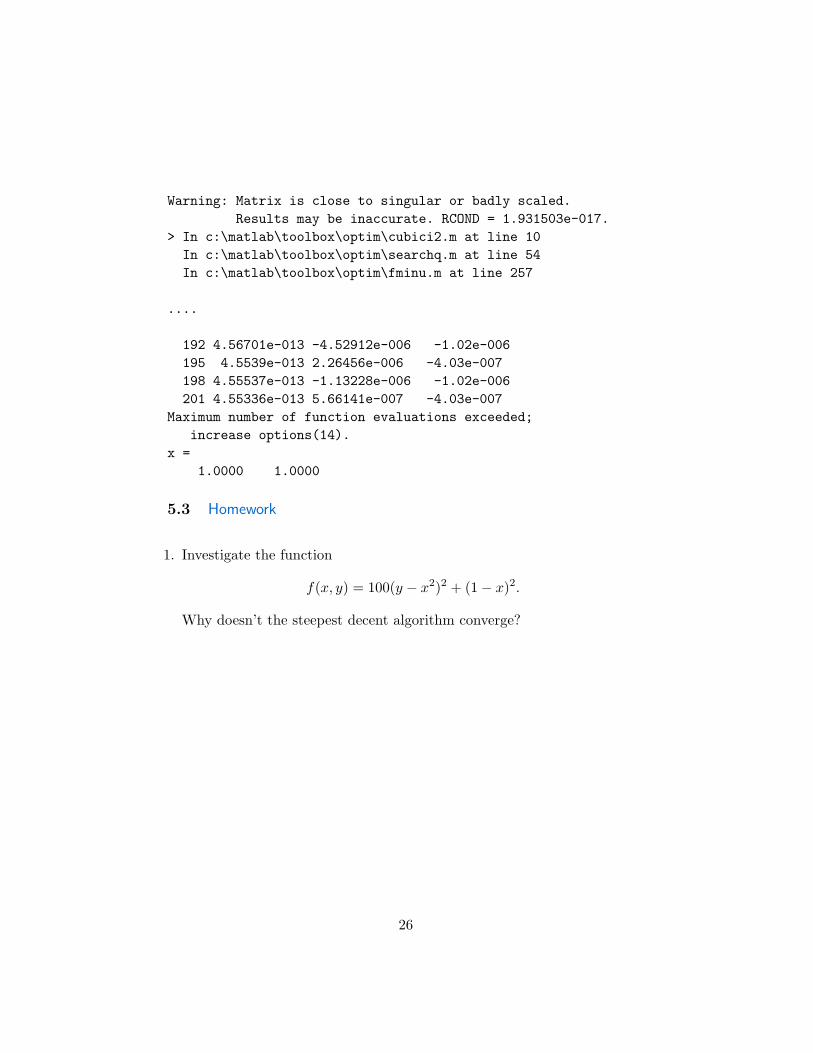
Warning: Matrix is close to singular or badly scaled.Results may be inaccurate. RCOND = 1.931503e-017.

> In c:\matlab\toolbox\optim\cubici2.m at line 10In c:\matlab\toolbox\optim\searchq.m at line 54In c:\matlab\toolbox\optim\fminu.m at line 257

....

192 4.56701e-013 -4.52912e-006 -1.02e-006195 4.5539e-013 2.26456e-006 -4.03e-007198 4.55537e-013 -1.13228e-006 -1.02e-006201 4.55336e-013 5.66141e-007 -4.03e-007

Maximum number of function evaluations exceeded;increase options(14).

x =1.0000 1.0000

5.3 Homework

1. Investigate the function

f(x, y) = 100(y − x2)2 + (1− x)2.

Why doesn’t the steepest decent algorithm converge?

26

6 Newton and quasi-Newton methods

6.1 Newton’s method

Based on the Taylor expansion

f(xn) ≈ f(xn) + f(xn)′(x− xn) +12

(x− xn)′f(xn)(x− xn)

one can derive, just as for the line-search problem, Newton’s method:

xn+1 = xn − (f(xn))−1f(xn).

Theorem 6.1 (Newton’s method) Assume the target function is in C3,x∗ is a local minimum, and the Hessian f(x∗) is positive definite. The if x0is close enough to x∗ then the order of convergence is at least 2.

Proof:

‖xn+1 − x∗‖ = ‖xn − x∗ − f(xn)−1f(xn)‖= ‖f(xn)−1[f(x∗)− f(xn)− f(xn)(x∗ − xn)]‖≤ C‖xn − x∗‖2,

for some constant C.A modification of this approach is to set

xn+1 = xn − αn(f(xn))−1f(xn),

where αn minimizes the function f(xn − α(f(xn))−1f(xn)).

6.2 Extensions

Consider the approach of choosing

xn+1 = xn − αnSnf(xn),

where Sn is some symmetric and positive-definite matrix and αn is the non-negative scalar that minimizes f(xn − αSnf(xn)). It can be shown thatsince Sn is positive-definite the algorithm is descending.

27

Assume

f(x) =12x′Qx− x′b =

12

(x− x∗)′Q(x− x∗)− 12x∗′Qx∗,

were Q a positive definite and symmetric matrix and x∗ = Q−1b is theminimizer of f . Note that in this case f(x) = Qx− b. and

f(xn−αSnf(xn)) =12

(xn−αSnf(xn))′Q(xn−αSnf(xn))−(xn−αSnf(xn))′b,

which is minimized at

αn =f(xn)′Snf(xn)

f(xn)′SnQSnf(xn).

It follows that

12

(xn+1 − x∗)′Q(xn+1 − x∗) =1− (f(xn)′Snf(xn))2

f(xn)′SnQSnf(xn)f(xn)′Q−1f(xn)

× 1

2(xn − x∗)′Q(xn − x∗).

Theorem 6.2 For the quadratic case

12

(xn+1 − x∗)′Q(xn+1 − x∗) ≤(Bn − bnBn + bn

)2 12

(xn − x∗)′Q(xn − x∗),

where Bn and bn are the largest and smallest eigenvalues of SQ.

6.3 The Davidon-Fletcher-Powell (DFP) method

This is a rank-two correction procedure. The algorithm starts with somepositive-definite algorithm S0, initial point x0:

1. Minimizes f(xn)−αSnf(xn) to obtain xn+1, ∆nx = xn+1−xn = −αnSnf(xn),f(xn+1) and ∆nf = f(xn+1)− f(xn).

2. Set

Sn+1 = Sn +∆nx′∆nx∆nx′∆nf

− Sn∆nf∆nf′Sn

∆nf ′Sn∆nf.

3. Go to 1.

28

It follows, since ∆nx′f(xn+1) = 0, that if Sn is positive definite then sois Sn+1.

Proof: Define ∆x = xn+1 − xn, ∆f = f(xn+1)− f(xn). Since

Sn+1 = Sn +(∆x)′(∆x)(∆x)′(∆f)

− Sn(∆f)(∆f)′Sn(∆f)′Sn(∆f)

,

it follows that

y′Sn+1y = y′Sny −(y′Sn(∆f))2

(∆f)′Sn(∆f)+

(y′(∆x))2

(∆x)′(∆f)

= a′a− (a′b)2

b′b+

(y′(∆x))2

(∆x)′(∆f), (1)

where a = S1/2n y and b = S

1/2n (∆f).

Next, since xn+1 is computed by minimizing the function f in the givendirection, it follows that (f(xn))′Sn(f(xn+1)). However, ∆x = −αnSnf(xn).It can be concluded that (∆x)′(∆f) = αn(f(x− n))′Sn(f(xn)) > 0.

The first difference in (1) is strictly positive, unless y ∝ (∆f). assumeit is. In which case the second term is proportional to (f(x−n))′Sn(f(xn)),thus positive.

6.4 The Broyden-Flecher-Goldfarb-Shanno (BFGS) method

In this method the Hessian is approximated. This is a rank-two correctionprocedure as well. The algorithm starts with some positive-definite algo-rithm H0, initial point x0:

1. Minimizes f(xn) − αH−1n f(xn) to obtain xn+1, ∆kx = xn+1 − xn =

−αnH−1n f(xn), f(xn+1) and ∆nf = f(xn+1)− f(xn).

2. Set

Hn+1 = Hn +∆nf

′∆nf

∆nf ′∆nx− Hn∆nx∆nx′Hn

∆nx′Hn∆nx.

3. Go to 1.

29

6.5 The function fminunc

FMINUNC Finds the minimum of a function of several variables.X=FMINUNC(FUN,X0) starts at the point X0 and finds a minimum

X of the function described in FUN. X0 can be a scalar, vector or matrix.The function FUN (usually an M-file or inline object) should return a scalarfunction value F evaluated at X when called with feval: F=feval(FUN,X).See the examples below for more about FUN.

X=FMINUNC(FUN,X0,OPTIONS) minimizes with the default optimiza-tion parameters replaced by values in the structure OPTIONS, an argumentcreated with the OPTIMSET function. See OPTIMSET for details. Usedoptions are Display, TolX, TolFun, DerivativeCheck, Diagnostics, GradObj,HessPattern,LineSearchType, Hessian, HessUpdate, MaxFunEvals, MaxIter, DiffMin-Change and DiffMaxChange, LargeScale, MaxPCGIter, PrecondBandWidth,TolPCG, TypicalX. Use the GradObj option to specify that FUN can becalled with two output arguments where the second, G, is the partial deriva-tives of the function df/dX, at the point X: [F,G] = feval(FUN,X). Use Hes-sian to specify that FUN can be called with three output arguments wherethe second, G, is the partial derivatives of the function df/dX, and the thirdH is the 2nd partial derivatives of the function (the Hessian) at the pointX: [F,G,H] = feval(FUN,X). The Hessian is only used by the large-scalemethod, not the line-search method.

X=FMINUNC(FUN,X0,OPTIONS,P1,P2,...) passes the problem-dependentparameters P1,P2,... directly to the function FUN, e.g. FUN would becalled using feval as in: feval(FUN,X,P1,P2,...). Pass an empty matrix forOPTIONS to use the default values.

[X,FVAL]=FMINUNC(FUN,X0,...) returns the value of the objectivefunction FUN at the solution X.

[X,FVAL,EXITFLAG]=FMINUNC(FUN,X0,...) returns a string EXIT-FLAG that describes the exit condition of FMINUNC. If EXITFLAG is: ¿0 then FMINUNC converged to a solution X. 0 then the maximum numberof function evaluations was reached. ¡ 0 then FMINUNC did not convergeto a solution.

[X,FVAL,EXITFLAG,OUTPUT]=FMINUNC(FUN,X0,...) returns a struc-ture OUTPUT with the number of iterations taken in OUTPUT.iterations,the number of function evaluations in OUTPUT.funcCount, the algorithmused in OUTPUT.algorithm, the number of CG iterations (if used) in OUT-PUT.cgiterations, and the first-order optimality (if used) in OUTPUT.firstorderopt.

[X,FVAL,EXITFLAG,OUTPUT,GRAD]=FMINUNC(FUN,X0,...) returns

30

the value of the gradient of FUN at the solution X.[X,FVAL,EXITFLAG,OUTPUT,GRAD,HESSIAN]=FMINUNC(FUN,X0,...)

returns the value of the Hessian of the objective function FUN at the solutionX.

6.6 Examples

Create a file myfun.m:

function f = myfun(x)f = 3*x(1)^2 + 2*x(1)*x(2) + x(2)^2; % cost function

Then call fminunc to find a minimum of ’myfun’ near [1,1]:

>> x0 = [1,1];>> [x,fval] = fminunc(’myfun’,x0)

After a couple of iterations, the solution, x, and the value of the function atx, fval, are returned:

x =1.0e-008 *-0.7914 0.2260

fval =1.5722e-016

To minimize this function with the gradient provided, modify the M-filemyfun.m so the gradient is the second output argument

function [f,g] = myfun(x)f = 3*x(1)^2 + 2*x(1)*x(2) + x(2)^2; % cost functionif nargout > 1

g(1) = 6*x(1)+2*x(2);g(2) = 2*x(1)+2*x(2);

end

and indicate the gradient value is available by creating an optimization op-tions structure with options.GradObj set to ’on’ using optimset:

>> options = optimset(’GradObj’,’on’);>> x0 = [1,1];>> [x,fval] = fminunc(’myfun’,x0,options)

31

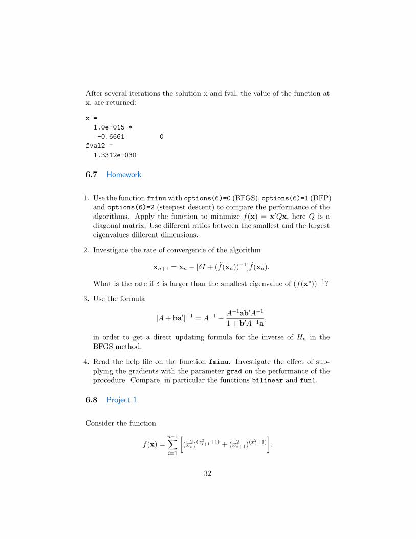
After several iterations the solution x and fval, the value of the function atx, are returned:

x =1.0e-015 *-0.6661 0

fval2 =1.3312e-030

6.7 Homework

1. Use the function fminu with options(6)=0 (BFGS), options(6)=1 (DFP)and options(6)=2 (steepest descent) to compare the performance of thealgorithms. Apply the function to minimize f(x) = x′Qx, here Q is adiagonal matrix. Use different ratios between the smallest and the largesteigenvalues different dimensions.

2. Investigate the rate of convergence of the algorithm

xn+1 = xn − [δI + (f(xn))−1]f(xn).

What is the rate if δ is larger than the smallest eigenvalue of (f(x∗))−1?

3. Use the formula

[A+ ba′]−1 = A−1 − A−1ab′A−1

1 + b′A−1a,

in order to get a direct updating formula for the inverse of Hn in theBFGS method.

4. Read the help file on the function fminu. Investigate the effect of sup-plying the gradients with the parameter grad on the performance of theprocedure. Compare, in particular the functions bilinear and fun1.

6.8 Project 1

Consider the function

f(x) =n−1∑i=1

[(x2i )

(x2i+1+1) + (x2

i+1)(x2i+1)

].

32

Use the function fminunc to identify local minima of the function. Try tothe procedure with and without providing the gradient. Try it for differentn’s. Which is the largest n for which the convergence was successful?

33

7 Constrained Minimization Conditions

The general (constrained) optimization problem has the form:

minx∈Rd

f(x)

subject to:

gi(x) = 0 i = 1, . . . ,me

gi(x) ≤ 0 i = me + 1, . . . ,mxl ≤ x ≤ xu

The first me constraints are called equality constraints and the last m−me

constraints are the inequality constraints.

7.1 Necessary conditions (equality constraints)

We assume first that me = m — all constraints are equality constraints.Let x∗ be a solution of the optimization problem. Let g = (g1, . . . , gm).Note that g is a (non-linear) transformation from Rd into Rm. The setx ∈ Rn : g(x) = 0 is a surface in Rn. This surface is approximated nearx∗ by x∗ +M , where

M = y : g(x∗)′y = 0.

In order for this approximation to hold, x∗ should be a regular point of theconstraint, i.e. (g1(x∗), . . . , gm(x∗)) should be linearly independent.

Theorem 7.1 (Lagrange multipliers) Let x∗ be a local extremum pointof f subject to the constraint g = 0. Assume that x∗ is a regular point ofthese constraints. Then there is a λ ∈ Rm such that

f(x∗) + g(x∗)λ = f(x∗) +m∑j=1

λj gj(x∗) = 0.

Given λ, one can consider the Lagrangian:

l(x, λ) = f(x) + g(x)λ.

34

The necessary conditions can be formulated as l = 0. The matrix of partialsecond derivatives of l (with respect to x) at x∗ is

lx(x∗) = f(x∗) + g(x∗)λ = f(x∗) +m∑j=1

gj(x∗)λj

We say that this matrix is positive semidefinite over M if x′ lx(x∗)x ≥ 0, forall x ∈M .

Theorem 7.2 (Second-order condition) Let x∗ be a local extremum pointof f subject to the constraint g = 0. Assume that x∗ is a regular point ofthese constraints, and let λ ∈ Rm be such that

f(x∗) + g(x∗)λ = f(x∗) +m∑j=1

λj gj(x∗) = 0.

Then the matrix lx(x∗) is positive semidefinite over M .

7.2 Examples

We now give some applications of the above theory.

Example 7.1 Minimize f(x, y, z) = xy+ yz+ xz, subject to x+ y+ z = 3.

The necessary conditions become:

y + z + λ = 0x+ z + λ = 0x+ y + λ = 0x+ y + z = 3.

Solving this system gives x = y = z = 1, λ = −2.

Example 7.2 A discrete random variable takes the values x1, . . . , xd, withprobabilities p1, . . . , pd. For a given mean value m, find the distributionwhich minimizes the entropy

f(p1, . . . , pd) = −d∑i=1

pi log(pi).

35

The problem can be formulated as

min f(p1, . . . , pd)

subject to:

d∑i=1

pi = 1,d∑i=1

xipi = m

0 ≤ pi, i = 1, . . . , d.

Ignoring the set-constraints, the Lagrangian becomes

l(p1, . . . , pd, λ1, λ2) =d∑i=1

−pi log(pi) + λ1pi + λ2xipi − λ1 −mλ2.

The necessary conditions are

− log(pi)− 1 + λ1 + λ2xi = 0, i = 1, . . . , d,

which leads to

pi = exp(λ1 − 1) + λ2xi,d∑i=1

pi = 1,d∑i=1

xiPi = m.

Note that the solution satisfies the set-constraints.

Example 7.3 A chain is suspended from two hooks that are t meters aparton a horizontal line. The chain consists of d links. Each link is 1 meterlong (measured from the inside). What is the shape of the chain?

We intend to minimize the potential energy of the chain. We let link i axi distance horizontally and yi distance vertically. The potential energy ofa link is its weight times its vertical distance (from some reference point).The potential energy of the chain is the sum of the potential energies of thelinks. Take the top as the reference and assume that the mass of each link isconcentrated at the center of the link. The potential energy is proportionalto

f(y1, . . . , yd) = 0.5y1 + (y1 + 0.5y2) + · · ·+ (y1 + · · ·+ yd−1 + 0.5yd)

=d∑i=1

(d− i+ 0.5)yi.

36

The constraints are:

d∑i=1

yi = 0,d∑i=1

xi =d∑i=1

√1− y2

i = t.

The first order necessary conditions are

(d− i+ 0.5) + λ1 −λ2yi

(1− y2i )1/2 = 0, for i = 1, . . . , d,

which leads toyi = − d− i+ 0.5 + λ1

[λ22 + (d− i+ 0.5 + λ1)2]1/2

.

7.3 Necessary conditions (inequality constraints)

We now consider the case where me < m. Let x∗ be a solution of theconstrained optimization problem. A constraint gj is active at x∗ if gj(x∗) =0 and it is inactive if gj(x∗) < 0. Note that all equality constraints are active.Denote by J the set of all active constraints.

For the consideration of necessary conditions when inequality constraintsare present the definition of a regular point should be extended. We say nowthat x∗ is regular if gj(x∗) : j ∈ J are linearly independent.

Theorem 7.3 (Kuhn-Tucker Conditions) Let x∗ be a local extremumpoint of f subject to the constraint gj(x) = 0, 1 ≤ j ≤ me and gj(x) ≤ 0,me + 1 ≤ j ≤ m. Assume that x∗ is a regular point of these constraints.Then there is a λ ∈ Rm such that λj ≥ 0, for all j > me, and

f(x∗) +m∑j=1

λj gj(x∗) = 0

m∑j=me+1

λjgj(x∗) = 0.

Let

lx(x∗) = f(x∗) +m∑j=1

λj gj(x∗).

37

Theorem 7.4 (Second-order condition) Let x∗ be a local extremum pointof f subject to the constraint gj(x) = 0, 1 ≤ j ≤ me and gj(x) ≤ 0,me+ 1 ≤ j ≤ m. Assume that x∗ is a regular point of these constraints, andlet λ ∈ Rm be such that λj ≥ 0, for all j > me, and

f(x∗) +m∑j=1

λj gj(x∗) = 0.

Then the matrix lx(x∗) is positive semidefinite on the tangent subspace ofthe active constraints.

7.4 Sufficient conditions

Sufficient conditions are based on second-order conditions:

Theorem 7.5 (Equality constraints) Suppose there is a point x∗ satis-fying g(x∗) = 0, and a λ ∈ Rm such that

f(x∗) +m∑j=1

λj gj(x∗) = 0.

Suppose also that the matrix lx(x∗) is positive definite on M . Then x∗ is astrict local minimum for the constrained optimization problem.

Theorem 7.6 (Inequality constraints) Suppose there is a point x∗ thatsatisfies the constraints. A sufficient condition for x∗ to be a strict localminimum for the constrained optimization problem is the existence of a λ ∈Rm such that λj ≥ 0, for me < j ≤ m, and

f(x∗) +m∑j=1

λj gj(x∗) = 0 (2)

m∑j=me+1

λjgj(x∗) = 0, (3)

and the Hessian matrix lx(x∗) is positive on the subspace

M ′ = y : gj(x∗)′y = 0, j ∈ J

where J = j : gj(x∗) = 0, λj > 0

38

Example 7.4 Consider the problem:

minimize 2x2 + 2xy + y2 − 10x− 10ysubject to x2 + y2 ≤ 5

3x+ y ≤ 6.

The first order necessary conditions are

4x+ 2y − 10 + 2λ13 + 3λ2 = 02x+ 2y − 10 + 2λ1y + λ2 = 0

λ1 ≥ 0, λ2 ≥ 0λ1(x2 + y2 − 5) = 0λ2(3x+ y − 6) = 0.

One should check different subsets of active and inactive constraints. Forexample, if we set J = 1 then

4x+ 2y − 10 + 2λ13 + 3λ2 = 02x+ 2y − 10 + 2λ1y + λ2 = 0

x2 + y2 = 5,

which has the solution x = 1, y = 2, λ1 = 1. This yields 3x + y = 5, andhence the second constraint is satisfied. Thus, since λ1 > 0, we concludethat this solution satisfies the first order necessary conditions.

7.5 Sensitivity

The Lagrange multipliers can be interpreted as the price of incrementalchange in the constraints. Consider the class of problems:

minimize f(x)subject to g(x) = c.

For each c, assume the existence of a solution point x∗(c). Under appropriateregularity conditions the function x∗(c) is well behaved with x∗(0) = x∗.

Theorem 7.7 (Sensitivity Theorem) Let f,g ∈ C2 and consider thefamily of problem defined above. Suppose that for c = 0 there is a localsolution x∗ that is a regular point and that, together with its associated La-grange multiplier vector λ, satisfies the second-order sufficient conditions for

39

a strict local minimum. Then for every c in a neighborhood of 0 there isx∗(c), continuous in c, such that x∗(0) = x∗, x∗(c) is a local minimum ofthe constrained problem indexed by c, and

f(x∗(c)) | c=0 = −λ.

7.6 Homework

1. Consider the constraints x1 ≥ 0, x2 ≥ 0 and x2−x1− 1)2 ≤ 0. Show that(1, 0) is feasible but not regular.

2. Find the rectangle of given perimeter that has greatest area by solvingthe first-order necessary conditions. Verify that the second-order sufficientconditions are satisfied.

3. Three types of items are to be stored. Item A costs one dollar, item B coststwo dollars and item C costs 4 dollars. The demand for the three itemsare independent and uniformly distributed in the range [0, 3000]. Howmany of each type should be stored if the total budget is 4,000 dollars?

4. Let A be an n×m matrix of rank m and let L be an n× n matrix thatis symmetric and positive-definite on the subspace M = y : Ay = 0.Show that the (n+m)× (n+m) matrix[

L A′

A 0

]is non-singular.

5. Consider the quadratic program

minimize x′Qx− 2b′x

subject to Ax = c.

Prove that x∗ is a local minimum point if and only if it is a global minimumpoint.

6. Maximize 14x− x2 + 6y − y2 + 7 subject to x+ y ≤ 2, x+ 2y ≤ 3.

40

8 Lagrange methods

The Lagrange methods for dealing with constrained optimization problemare based on solving the Lagrange first-order necessary conditions. In par-ticular, for solving the problem with equality constraints only:

minimize f(x)subject to g(x) = 0,

the algorithms look for solutions of the problem:

f(x) +m∑j=1

λj gj(x) = 0

g(x) = 0,

8.1 Quadratic programming

An important special case is when the target function f is quadratic andthe constraints are linear:

minimize (1/2)x′Qx + x′c

subject to a′ix = bi, 1 ≤ i ≤ me

a′ix ≤ bi, me + 1 ≤ i ≤ m

with Q a symmetric matrix.

8.1.1 Equality constraints

In the particular case where me = m the above becomes

minimize (1/2)x′Qx + x′c

subject to Ax = b.

and the Lagrange necessary conditions become

Qx +A′λ+ c = 0

Ax− b = 0.

This system is nonsingular if Q is positive definite on the subspace M =x : Ax = 0. If Q is nonsingular then the solution becomes:

x = Q−1A′(AQ−1A′)−1[AQ−1c + b]−Q−1c

λ = −(AQ−1A′)−1[AQ−1c + b].

41

8.1.2 Inequality constraints

For the general quadratic programming problem, the method of active set isused. A working set of constraints Wn is updated in each iteration. The setWn contains all constraints that are suspected to satisfy an equality relationat the solution point. In particular, it contains the equality constraints. Analgorithm for solving the general quadratic problem is:

1. Start with a feasible point x0 and a working set W0. Set n = 0

2. Solve the quadratic problem

minimize (1/2)d′Qd + (c +Qxn)′dsubject to a′id = 0, i ∈Wn.

If d∗n = 0 go to 4.

3. Set xn+1 = αnd∗n, where

αn = mina′id∗n>0

1,bi − a′ixn

a′id∗n

.

If αn < 1, adjoin the minimizing index above to Wn to form Wn+1. Setn = n+ 1 and return to step 2.

4. Compute the Lagrange multiplier in step 3 and let λn = minλi : i ∈Wn, i > me. If λn ≥ 0, stop; xn is a solution. Otherwise, drop λn fromWn to form Wn+1 and return to step 2.

Example 8.1 Consider the problem

minimize 2x2 + xy + y2 − 12x− 10ysubject to (1) x+ y ≤ 0,

(2) − x ≤ 0,(3) − y ≤ 0.

Take x0 = (0, 0)′, and W0 = 2, 3. Then d∗0 = (0, 0)′. Both Lagrangemultipliers are negative, but the one corresponding to (2) is more negative.Drop that constraint, and put W1 = 3. Minimizing along the line y = 0leads to x1 = (3, 0)′. The Lagrange multiplier of the active constraint isnegative, thus W2 = ∅. Also, d∗1 = (−1, 4), the direction to the overalloptimum at (2, 4)′. We move to the constraint (1), and write W3 = (1).Finally, we move along this constraint to the solution.

42

8.2 Sequential Quadratic Programming

Let us go back to the general problem

minimize f(x)subject to gi(x) = 0, i = 1, . . . ,me

gi(x) ≤ 0, i = me + 1, . . . ,m.

The SQP method solves this problem by solving a sequence of QP problemswhere the Lagrangian function l is approximated by a quadratic functionand the constraints are approximated by a linear hyper-space.

8.3 Newton’s Method

Consider the case of equality constraints only. At each iteration the problem

minimize (1/2)d′ lx(xn, λn)d + l(xn, λn)′dsubject to gi(xn)′d + gi(xn) = 0, i = 1, . . . ,m

is solved. It can be shown that the rate of convergence of this algorithmis 2 (at least) if the starting point (x0, λ0) is close enough to the solution(x∗, λ∗). A disadvantage of this approach is the need to compute Hessian.

8.4 Structured Methods

These methods are modifications of the basic Newton method, with approx-imations replacing Hessian. One can rewrite the solution to the Newton stepin the form [

xn+1λn+1

]=[

xnλn

]−[ln g′ngn 0

]−1[ lngn

].

Instead, one can use the formula[xn+1λn+1

]=[

xnλn

]− αn

[Hn g′ngn 0

]−1[ lngn

],

with αn and Hn appropriately chosen.

43

8.5 Merit function

In order to choose the αn and to assure that the algorithm will convergea merit function is associated with the problem such that a solution ofthe constrained problem is a (local) minimum of the merit function. Thealgorithm should be descending with respect to the merit function.

Consider, for example, the problem with inequality constraints only:

minimize f(x)subject to gi(x) ≤ 0, i = 1, . . . ,m.

The absolute-value merit function is given by

Z(x) = f(x) + cm∑i=1

gi(x)+.

The parameter α is chosen by minimizing the merit function in the directionchosen by the algorithm.

Theorem 8.1 If H is positive-definite and if c > max1≤i≤m λi then thealgorithm is descending with respect to the absolute-value merit function.

Proof: The optimization problem is solved by solving sequentially problemsof the form:

minimize (1/2)d′Hd + f(x)′dsubject to gj(x)′d + gj(x) ≤ 0, i = 1, . . . ,m,

The necessary conditions here are

Hd + f(x) +m∑j=1

λj gj(x) = 0 (4)

gj(x)′d + gj(x) ≤ 0 (5)λj [gj(x) + gj(x)] = 0 (6)

λj ≥ 0. (7)

Let J(x) = gi(x) > 0. Now, for α > 0,

Z(x + αd) = f(x + αd) + cm∑i=1

gi(x + αd)+

44

= f(x) + αf(x)′d + cm∑i=1

[gi(x)+ + αcgj(x)′d + o (α)]+

= f(x) + αf(x)′d + cm∑i=1

gi(x)+ + αc∑

j∈J(x)

gj(x)′d + o (α)

= Z(x) + αf(x)′d + αc∑

j∈J(x)

gj(x)′d + o (α) .

Here we applied condition (5) in order to infer that gj(x)′d ≤ 0 if gj(x) = 0.Using this condition again we get

c∑

j∈J(x)

gj(x)′d ≤ c∑

j∈J(x)

−gj(x) = −cm∑j=1

gj(x)+. (8)

Using (4) we can infer that

f(x)′d = −d′Hd−m∑j=1

λj gj(x)d,

which by using condition (6) leads to

f(x)′d ≤ −d′Hd +m∑j=1

λjgj(x)+ ≤ −d′Hd + maxjλj

m∑j=1

gj(x)+. (9)

Summarizing what we got thus far leads to

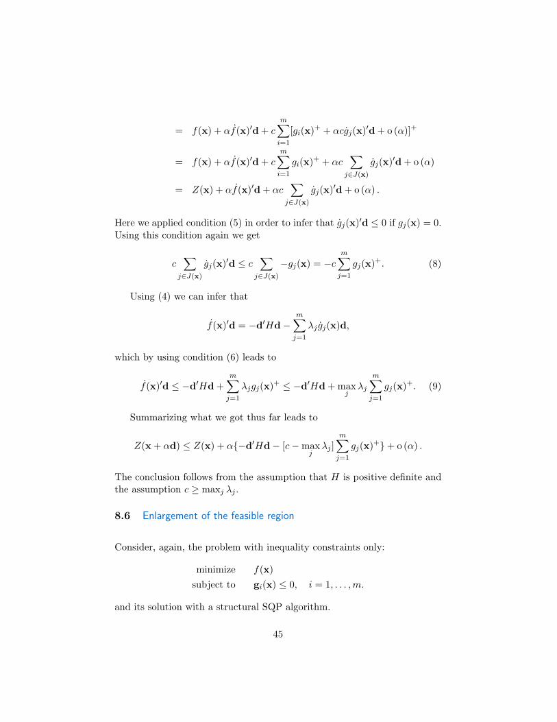
Z(x + αd) ≤ Z(x) + α−d′Hd− [c−maxjλj ]

m∑j=1

gj(x)++ o (α) .

The conclusion follows from the assumption that H is positive definite andthe assumption c ≥ maxj λj .

8.6 Enlargement of the feasible region

Consider, again, the problem with inequality constraints only:

minimize f(x)subject to gi(x) ≤ 0, i = 1, . . . ,m.

and its solution with a structural SQP algorithm.

45

Assume that at the current iteration xn = x and Hn = H. Then onewants to consider the QP problem:

minimize (1/2)d′Hd + f(x)subject to gi(x)′d + g(x) ≤ 0, i = 1, . . . ,m.

However, it is possible that this problem is infeasible at the point x. Hence,the original method breaks down. However, one can consider instead theproblem

minimize (1/2)d′Hd + f(x) + cm∑i=1

ξi

subject to gi(x)′d + g(x) ≤ ξi, i = 1, . . . ,m.−ξi ≤ 0, i = 1, . . . ,m,

which is always feasible.

Theorem 8.2 If H is positive-definite and if c > max1≤i≤m λi then thealgorithm is descending with respect to the absolute-value merit function.

8.7 The Han–Powell method

The Han–Powell method is what is used by Matlab for SQP. It is a Quasi-Newton method, where Hn is updated using the BFGS approach:

Hn+1 = Hn +(∆l)(∆l)′

(∆x)′(∆l)− Hn(∆x)(∆x)′Hn

(∆x)′Hn(∆x),

where∆x = xn+1 − xn, ∆l = l(xn+1, λn+1)− l(xn, λn).

It can be shown that Hn+1 is positive-definite if Hn is and if (∆x)′(∆l) > 0.

8.8 Constrained minimization in Matlab

Write the M-file fun2.m:

function [f,g]=fun2(x)f = exp(x(1))*(4*x(1)^2+2*x(2)^2+4*x(1)*x(2)+2*x(2)+1);g(1,1) = 1.5 + x(1)*x(2) - x(1) - x(2);g(2,1) = -x(1)*x(2) - 10;

46

and run the Matlab session:

>> x0 = [-1,1];>> x = constr(’fun4’, x0)x =

-9.5474 1.0474>> [f,g] = fun4(x)f =

0.0236g =1.0e-014 *

0.1110-0.1776

>> options = [];>> vlb = [0,0];>> vlu = [];>> x = constr(’fun4’, x0, options, vlb, vlu)x =

0 1.5000>> [f,g] = fun4(x)f =

8.5000g =

0-10

Write the M-file grodf4.m:

function [df,dg] = grudf4(x)f = exp(x(1))*(4*x(1)^2+2*x(2)^2+4*x(1)*x(2)+2*x(2)+1);df = [f + exp(x(1))*(8*x(1) + 4*x(2)), exp(x(1))*(4*x(1) + 4*x(2) + 2)];dg = [x(2) - 1, -x(2); x(1) - 1, -x(1)];

and run the session:

>> vlb = [];>> x = constr(’fun4’, x0, options, vlb, vlu, ’grudf4’)x =

-9.5474 1.0474

8.9 Constrained minimization in Matlab (using the function fmincon

47

Let us consider the problem:

minimize f(x) = ex1(4x21 + 2x2

2 + 4x1x2 + 2x2 + 1)subject to 1.5 + x1x2 − x1 − x2 ≤ 0

−x1x2 ≤ 10

First create the M-files obj5.m

function f = obj5(x)f=exp(x(1)) * (4*x(1)^2 + 2*x(2)^2 + 4*x(1)*x(2) + 2*x(2) + 1);

and con5.m:

function [c, ceq] = con5(x)c = [1.5 + x(1)*x(2) - x(1) - x(2);

-x(1)*x(2) - 10];ceq = [];

In the command window do:

>> x0 = [-1 1];>> options = optimset(’LargeScale’,’off’,’Display’,’iter’);>> [x,fval,exitflag,output] = fmincon(’obj5’,x0,[],[],[],[],[],[],...’con5’,options);

max DirectionalIter F-count f(x) constraint Step-size derivative Procedure

1 3 1.8394 0.5 1 0.04862 7 1.85127 -0.09197 1 -0.556 Hessian modified twice3 11 0.300167 9.33 1 0.174 15 0.529834 0.9209 1 -0.9655 20 0.186965 -1.517 0.5 -0.1686 24 0.0729085 0.3313 1 -0.05187 28 0.0353322 -0.03303 1 -0.01428 32 0.0235566 0.003184 1 -6.22e-0069 36 0.0235504 9.032e-008 1 1.76e-010 Hessian modified

Optimization terminated successfully:Search direction less than 2*options.TolX andmaximum constraint violation is less than options.TolConActive Constraints:

12

>> x

48

x =-9.5474 1.0474

>> valfval =

0.0236>> [c, ceq] = con5(x)c =1.0e-014 *

0.1110-0.1776

ceq =[]

>> output.funcCountans =

38

The above problem can be solved more efficiently and accurately if gra-dients are supplied by the user. Create the M-files:

function [f, G] = obj5grad(x)f =exp(x(1)) * (4*x(1)^2 + 2*x(2)^2 + 4*x(1)*x(2) + 2*x(2) + 1);t = exp(x(1))*(4*x(1)^2+2*x(2)^2+4*x(1)*x(2)+2*x(2)+1);G = [ t + exp(x(1)) * (8*x(1) + 4*x(2)),

exp(x(1))*(4*x(1)+4*x(2)+2)];

and

function [c, ceq, dc, dceq] = con5grad(x)c = [1.5 + x(1)*x(2) - x(1) - x(2);

-x(1)*x(2) - 10];dc = [x(2)-1, -x(2);

x(1)-1, -x(1)];ceq = [];dceq = [];

In the command window:

>> x0x0 =

-1 1>> options = optimset(’LargeScale’,’off’);>> options = optimset(options,’GradObj’,’on’,’GradConstr’,’on’);

49

>> [x,fval,exitflag,output] = fmincon(’obj5grad’,x0,[],[],[],[],[],[],...>> ’con5grad’,options);Optimization terminated successfully:Search direction less than 2*options.TolX andmaximum constraint violation is less than options.TolConActive Constraints:

12

>> xx =

-9.5474 1.0474>> fvalfval =

0.0236>> [c, ceq] = con5grad(x)c =1.0e-014 *

0.1110-0.1776

ceq =[]

>> output.funcCountans =

20

8.10 Homework

1. Read the help files of the functions constr and fmincon. Redo the ex-ample given in class with the function fmincon. Compare the propertiesof the two functions in QP problems of different magnitude.

2. Let H be a positive-definite matrix and assume that, throughout somecompact set, the quadratic programing has a unique solution, such thatthe Lagrange multipliers are not larger than c. Let xn : n ≥ 0 bea sequence generated by the recursion xn+1 = xn + αndn, where d isthe direction found by solving the QP centered at xn and with H fixedand αn is determined by minimization of the function Z. Show that anylimit point of xn satisfies the first order necessary conditions for theconstrained minimization problem.

50

3. Extend the result in 2 for the case where H = Hn changes but yet ε‖x‖2 ≤x′Hnx ≤ c‖x‖2 for some 0 < ε < c <∞ and for all x and n.

51

9 Large scale problems

9.1 Basic issues

Large scale problems requires special techniques to deal with memory prob-lems and numeric complications.

Consider the issue in the context of unconstrained minimization of afunctionf(x). The basic approaches to minimization of a function can by thegeneral heuristic: Define a neighborhood N of the current x. Approximatethe function f by a function q over N . The solution to the minimizationproblem in q provides a candidate for a new x, x + d. This candidateis adopted if f(x + d) < f(x). (For example, q(d) = f(x) + f(x)′d +(1/2)d′f(x)d and N = ‖Dd‖ ≤ ε, for D a diagonal scaling matrix.)

However, when the dimension of the problem is large this approach isnot feasible. The alternative which is used in MATLAB is to choose a twodimensional subspace S and to constraint the analysis to that subspace.The subspace is formed by taking the direction of the gradient and eitherthe Newton direction, i.e. the solution to

f(x)d2 = −f(x),

or a direction of negative curvature

d′2f(x)d2 < 0

(in order to force convergence).Large scale algorithms will work better if they are provided with the

Hessian. The main issue in the limitations on the memory involves storageof that matrix. In many applications, however, it follows that many of theentries in the matrix are actually zeros. Room can be saved by storing thematrix in the sparse matrix form. Hence,

>> sparse(1:5,1:5,1)ans =

(1,1) 1(2,2) 1(3,3) 1(4,4) 1(5,5) 1

is a compact way to store the 5× 5 identity matrix.

52

9.2 Minimization with no constraints. Hassien provided

Let consider the function which was analyzed as part of the first project:

f(x) =n−1∑i=1

[(x2i )

(x2i+1+1) + (x2

i+1)(x2i+1)

].

Let us first minimize this function with the sparse tridiagonal Hessianmatrix. Start with the M-file brownfgh.m:

function [f,g,H] = brownfgh(x)

% Evaluate the function.n=length(x); y=zeros(n,1);i=1:(n-1);y(i)=(x(i).^2).^(x(i+1).^2+1)+(x(i+1).^2).^(x(i).^2+1);f=sum(y);

%% Evaluate the gradient.if nargout > 1

i=1:(n-1); g = zeros(n,1);g(i)= 2*(x(i+1).^2+1).*x(i).*((x(i).^2).^(x(i+1).^2))+...

2*x(i).*((x(i+1).^2).^(x(i).^2+1)).*log(x(i+1).^2);g(i+1)=g(i+1)+...

2*x(i+1).*((x(i).^2).^(x(i+1).^2+1)).*log(x(i).^2)+...2*(x(i).^2+1).*x(i+1).*((x(i+1).^2).^(x(i).^2));

end%% Evaluate the (sparse, symmetric) Hessian matrixif nargout > 2

v=zeros(n,1);i=1:(n-1);v(i)=2*(x(i+1).^2+1).*((x(i).^2).^(x(i+1).^2))+...

4*(x(i+1).^2+1).*(x(i+1).^2).*(x(i).^2).*((x(i).^2).^((x(i+1).^2)-1))+...2*((x(i+1).^2).^(x(i).^2+1)).*(log(x(i+1).^2));

v(i)=v(i)+4*(x(i).^2).*((x(i+1).^2).^(x(i).^2+1)).*((log(x(i+1).^2)).^2);v(i+1)=v(i+1)+...

2*(x(i).^2).^(x(i+1).^2+1).*(log(x(i).^2))+...4*(x(i+1).^2).*((x(i).^2).^(x(i+1).^2+1)).*((log(x(i).^2)).^2)+...2*(x(i).^2+1).*((x(i+1).^2).^(x(i).^2));

53

v(i+1)=v(i+1)+4*(x(i).^2+1).*(x(i+1).^2).*(x(i).^2).*((x(i+1).^2).^(x(i).^2-1));v0=v;v=zeros(n-1,1);v(i)=4*x(i+1).*x(i).*((x(i).^2).^(x(i+1).^2))+...

4*x(i+1).*(x(i+1).^2+1).*x(i).*((x(i).^2).^(x(i+1).^2)).*log(x(i).^2);v(i)=v(i)+ 4*x(i+1).*x(i).*((x(i+1).^2).^(x(i).^2)).*log(x(i+1).^2);v(i)=v(i)+4*x(i).*((x(i+1).^2).^(x(i).^2)).*x(i+1);v1=v;i=[(1:n)’;(1:(n-1))’];j=[(1:n)’;(2:n)’];s=[v0;2*v1];H=sparse(i,j,s,n,n);H=(H+H’)/2;

end

To better understand the structure of H, note that

>> n = 5;>> v0=ones(n,1);>> v1=ones(n-1,1);>> s=[v0;2*v1];>> i=[(1:n)’;(1:(n-1))’];>> j=[(1:n)’;(2:n)’];>> H=sparse(i,j,s,n,n);>> full(H)ans =

1 2 0 0 00 1 2 0 00 0 1 2 00 0 0 1 20 0 0 0 1

Continue with the real thing:

>> n = 1000;>> xstart = -ones(n,1);>> xstart(2:2:n,1) = 1;>> options = optimset(’GradObj’, ’on’, ’Hessian’, ’on’);> [x, fval, exitflag, output] = fminunc(’brownfgh’,xstart,options);Optimization terminated successfully:First-order optimality less than OPTIONS.TolFun, and no negative/zero

54

curvature detected>> exitflagexitflag =

1>> fvalfval =2.8709e-017

>> output.iterationsans =

8

9.3 Minimization with no constraints. Hassien not provided

Now, lets redo the problem, but without the Hessian. The algorithm willapproximate it, using the sparse finite-differences. Note that the gradientmust be provided in large-scale problems. Start with the M-file brownfg.m:

function [f,g] = brownfg(x)% Evaluate the function.n=length(x); y=zeros(n,1);i=1:(n-1);y(i)=(x(i).^2).^(x(i+1,1).^2+1)+(x(i+1).^2).^(x(i).^2+1);f=sum(y);

%% Evaluate the gradient if nargout > 1if nargout > 1

i=1:(n-1); g = zeros(n,1);g(i)= 2*(x(i+1).^2+1).*x(i).*((x(i).^2).^(x(i+1).^2))+...

2*x(i).*((x(i+1).^2).^(x(i).^2+1)).*log(x(i+1).^2);g(i+1)=g(i+1)+...

2*x(i+1).*((x(i).^2).^(x(i+1).^2+1)).*log(x(i).^2)+...2*(x(i).^2+1).*x(i+1).*((x(i+1).^2).^(x(i).^2));

end

The sparsity structure of H must be predetermined and provided.

>> i=[(1:n)’;(1:(n-1))’];>> j=[(1:n)’;(2:n)’];>> v0=ones(n,1);>> v1=ones(n-1,1);

55

>> s=[v0;v1];>> H=sparse(i,j,s,n,n);>> Hstr = (H + H’)/2;>> spy(Hstr);

Back to the optimization problem:

>> options = optimset(’GradObj’, ’on’, ’HessPattern’, Hstr);>> [x, fval, exitflag, output] = fminunc(’brownfg’,xstart,options);Optimization terminated successfully:First-order optimality less than OPTIONS.TolFun, and no negative/zerocurvature detected

>> exitflagexitflag =

1>> fvalfval =7.4739e-017

>> output.iterationsans =

8

9.4 Minimization with constraints.

The large-scale method for fmincon can handle equality constraints if noother constraints exist. Lets add to the problem 100 linear equality con-straints of the form Ax = b, where A is a 100 × 1000 matrix and b is a100-vector. They are given in the MAT-file browneq.mat.

>> load browneq>> spy(Aeq)>> condest(Aeq*Aeq’)ans =2.9310e+006

The function condest compute a 1-norm condition number estimate. If thenumber is large, it indicates that the matrix is close to being null.

>> options = optimset(’GradObj’, ’on’, ’Hessian’,’on’);>> [x, fval, exitflag, output] = fmincon(’brownfgh’,xstart,...[], [], Aeq, beq, [], [], [], options);

56

Optimization terminated successfully:Relative function value changing by less than OPTIONS.TolFun

>> fvalfval =205.9313

>> output.iterationsans =

22

9.5 Project 2

The goal is to minimize the function

f(x) = 1 +n∑i=1

[(3− 2xi)xi − xi−1 − xi+1 + 1]4 +n/2∑i=1

[xi + xi+n/2]4,

for an n which is a multiple of 4, and x0 = xn+1 = 0. Solve this both as amedium-scale problem (say, n = 8 or n = 16) and as a large-scale problem(say, n = 800). Try to find, on your machine, when the problem cannot besolved as a medium-scale and large-scale algorithms must be applied.

57

10 Penalty and Barrier Methods

The basic approach in these methods is to solve a sequence of unconstrainedproblems. The solutions of these problems converge to the solution of theoriginal problem.

10.1 Penalty method

Consider the problem

minimize f(x)subject to gi(x) ≤ 0, i = 1, . . . ,m.

Choose a continuous penalty function which is zero inside the feasible setand positive outside of it. For example,

P (x) = (1/2)m∑i=1

max0, gi(x)2.

Minimize, for each c, the problem

q(c,x) = f(x) + cP (x).

When c is increased it expected that the solution x∗(c) converges to x∗.

Lemma 10.1 Let cn+1 > cn, then

q(cn,x∗n) ≤ q(cn+1,x∗n+1) (10)P (x∗n) ≥ P (x∗n+1) (11)f(x∗n) ≤ f(x∗n+1). (12)

Proof:

q(cn+1,x∗n=1) = f(x∗n+1) + cn+1P (x∗n+1) ≥ f(x∗n+1) + cnP (x∗n+1)≥ f(x∗n) + cnP (x∗n) = q(cn,x∗n),

which proves (10). Also,

f(x∗n) + cnP (x∗n) ≤ f(x∗n+1) + cnP (x∗n+1)f(x∗n+1) + cn+1P (x∗n+1) ≤ f(x∗n) + cn+1P (x∗n).

58

Adding (13) and (13) yields

(cn+1 − cn)P (x∗n+1) ≤ (cn+1 − cn)P (x∗n),

which proves (11). Finally,

f(x∗n+1) + cnP (x∗n+1) ≥ f(x∗n) + cnP (x∗n),

which proves (12).

Lemma 10.2 Let x∗ be the solution of the original problem. Then for eachn

f(x∗) ≥ q(cn,x∗n) ≥ f(x∗n).

Proof:

f(x∗) = f(x∗) + cnP (x∗) ≥ f(x∗n) + cnP (x∗n) ≥ f(x∗n).

Theorem 10.1 Let xn be a sequence generated by the penalty method.Then, any limit point of the sequence is a solution to the original problem.

Proof: Suppose the subsequence x∗n : n ∈ N is a convergent subsequencewith limit x. The by continuity of f ,

limn∈N

f(x∗n) = f(x). (13)

Let f∗ be the optimal value associated with the problem. then accordingto Lemmas 10.1 and 10.2, the sequence of values q(cn,x∗n) is nondecreasingand bounded by f∗. Thus

limn∈N

q(cn,x∗n) = q∗ ≤ f∗. (14)

Subtracting (13) from (14) yields

limn∈N

cnP (x∗n) = q∗ − f(x). (15)

Since P (x∗n) ≥ 0 and cn → ∞, this implies limn∈N P (x∗n) = 0. By thecontinuity of P , P (x) = 0, thus x is feasible for the problem.

To show that x is optimal note that form Lemma 10.2, f(x∗n) ≤ f∗ andf(x) = limn∈N f(x∗n) ≤ f∗.

59

10.2 Barrier method

Consider again the problem

minimize f(x)subject to gi(x) ≤ 0, i = 1, . . . ,m,

and assume that the feasible set is the closure of its interior. A barrierfunction is a continuous and positive function over the feasible set whichgoes to ∞ as x approaches the boundary. For example,

B(x) =m∑i=1

1gi(x)

.

Minimize, for each c, the problem

minimize r(c,x) = f(x) +1cB(x)

subject to gi(x) ≤ 0, i = 1, . . . ,m.

Note that a method of unconstrained minimization can be used becausethe solution is in the interior of the feasible set. When c is increased it isexpected that the solution x∗(c) converges to x∗.

Theorem 10.2 Let xn be a sequence generated by the barrier method.Then, any limit point of the sequence is a solution to the original problem.

60