Nonlinear Optimization in AMPL with LGO

Nonlinear Optimization in AMPL with LGO

Presented by

János D. Pintér

Lecture Topics

• Introduction

• Continuous Nonlinear Optimization Model

• AMPL-LGO Solver Engine

• Illustrative Nonlinear Optimization Applications

• Conclusions and Illustrative References

• Comments and questions welcome! Further information available

2

Introducing Myself (Quickly)

• Education and professional background

M.Sc., Eötvös Loránd University (ELTE, Budapest): applied mathematics / operations research

Ph.D., Moscow State University: stochastic optimization

D.Sc., Hungarian Academy of Sciences: global optimization

• Hungarian-Canadian; living and working in the USA since 2016

• Lifelong interest in modeling and solving decision problems inspired by the real world

• Teaching management science / operations research / industrial and system engineering courses

• Presented training courses, and worked as a scientist / consultant / lecturer in cca. 40 countries

• Optimization software developer, doing research and teaching with AMPL

3

Introduction 2

• Author of a research monograph, a university textbook, a tutorial book and an e-book; editor of 7 books (as of 2020); further work on two book projects in progress

• Author/co-author of 200+ articles, book chapters, technical reports,…

• Professional society officer (past or present): Hung. Acad. Sci., INFORMS, EUROPT

• Editorial board member (present): J. of Global Optimization, Operations Research Forum, SpringerBriefs in Optimization (and several other journals in the past)

• Professional summary information: https://engineering.lehigh.edu/faculty/janos-d-pinter (link to change in September 2020) https://scholar.google.com/citations?user=iHrfmDEAAAAJ

“May you live interesting times!” Indeed, almost never had a boring moment...☺

4

https://engineering.lehigh.edu/faculty/janos-d-pinter

https://scholar.google.com/citations?user=iHrfmDEAAAAJ

Optimization Paradigm

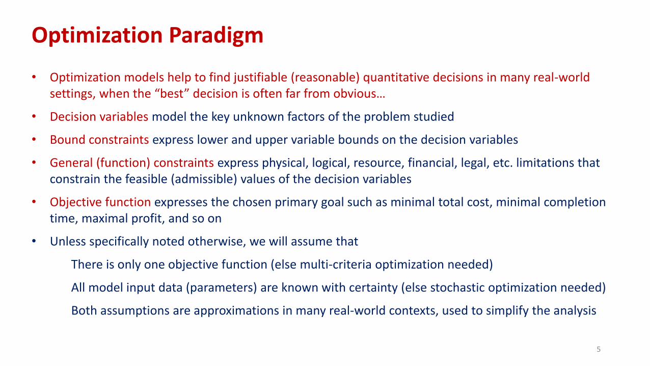
• Optimization models help to find justifiable (reasonable) quantitative decisions in many real-world settings, when the “best” decision is often far from obvious…

• Decision variables model the key unknown factors of the problem studied

• Bound constraints express lower and upper variable bounds on the decision variables

• General (function) constraints express physical, logical, resource, financial, legal, etc. limitations that constrain the feasible (admissible) values of the decision variables

• Objective function expresses the chosen primary goal such as minimal total cost, minimal completion time, maximal profit, and so on

• Unless specifically noted otherwise, we will assume that

There is only one objective function (else multi-criteria optimization needed)

All model input data (parameters) are known with certainty (else stochastic optimization needed)

Both assumptions are approximations in many real-world contexts, used to simplify the analysis

5

Optimization Model Development

General framework

Optimize system performance min f(x) x = (x1,…,xn) f: Rn → R

Subject to s.t.

Constraints (functions) g(x) 0 gj(x) 0, j = 1,…,m g: Rn → Rm

Bound constraints xl x xu xl , x , xu Rn

This concise model statement can be flexibly specified to describe decision-making scenarios, using corresponding model forms such as LP, ILP, MILP, NLO, MINLP, SP,…

A vast range of optimization applications in business, engineering, sciences

6

• Optimization model: min f(x) s.t. x D := { xl x xu , g(x) 0 }

• We will assume that at least some of the functions f and gj j = 1,…,m are nonlinear

• Key analytical assumptions

Bounds xl, xu are finite and known

Feasible set D is non-empty

All model functions f and g (component-wise) are continuous

• These analytical conditions are sufficient to guarantee the existence of the global solution set X*

• Local optimization (LO): we assume to have access to a high quality initial solution guess which can be sufficiently improved locally, to arrive at a good or provably optimal local solution; global optimality is guaranteed e.g., by model convexity (f and gj j = 1,…,m are all convex) when applicable

• Global optimization (GO): we assume that the model could have multiple optima of different quality, and we aim for the best of the local optima, the global solution x* (or global solution set X*)

Continuous Nonlinear Optimization Model

7

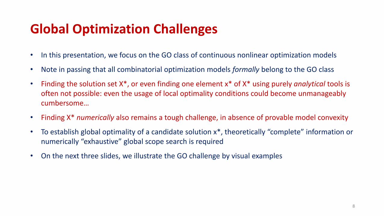
• In this presentation, we focus on the GO class of continuous nonlinear optimization models

• Note in passing that all combinatorial optimization models formally belong to the GO class

• Finding the solution set X*, or even finding one element x* of X* using purely analytical tools is often not possible: even the usage of local optimality conditions could become unmanageably cumbersome…

• Finding X* numerically also remains a tough challenge, in absence of provable model convexity

• To establish global optimality of a candidate solution x*, theoretically “complete” information or numerically “exhaustive” global scope search is required

• On the next three slides, we illustrate the GO challenge by visual examples

Global Optimization Challenges

8

An Illustrative Collection of Box-constrained Models

These are very small problems: n = 2, m= 0

However, some are already non-trivial GO challenges…

Numerical difficulties could rapidly increase as n, m become larger…

9

Some Hard(er) GO Test Problems

0

5

10

4.5

5

5.5

-30

-20

-10

0

0

5

10

-4

-2

0

2

4

-4

-2

0

2

4

0

5

10

15

-4

-2

0

2

4

-10

-5

0

5

10-10

-5

0

5

10

-20

0

20

-10

-5

0

5

10 10

What can be expected from GO software? Global scope search is key to numerical success…

GO Challenges Implied by Feasible Sets

1. Convex: OK (easy) 2. Non-convex: ? 3. Disconnected: ???

Again, what can we expect from software when solving models which have difficult feasible sets?

Traditional local optimization approaches could (and often will) fail in cases like 2 or 3; global search needed

11

Nonlinear Models: Modeling and Solver Difficulties

• No definite outcome, when solving new, “unusual”, or notoriously hard models

• It may be difficult to find even a reasonable initial solution: e.g., nonlinear equations

• It is often difficult to satisfy nonlinear (especially equality) constraints

• It could be difficult to maintain feasibility in non-convex models

• More complicated theory, many non-equivalent approaches (implemented in solver engines) to tackle hard nonlinear optimization problems

• Different starting solutions (“initial guesses”) can lead to different solutions reported by solver engines: this is typically due to non-convex model structure – and it often happens when we try to use local scope solvers to handle hard GO problems…

12

AMPL for Optimization Model Development

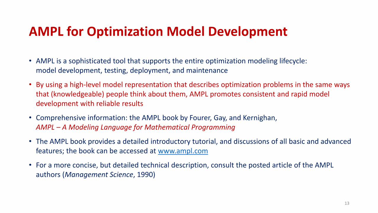
• AMPL is a sophisticated tool that supports the entire optimization modeling lifecycle: model development, testing, deployment, and maintenance

• By using a high-level model representation that describes optimization problems in the same ways that (knowledgeable) people think about them, AMPL promotes consistent and rapid model development with reliable results

• Comprehensive information: the AMPL book by Fourer, Gay, and Kernighan, AMPL – A Modeling Language for Mathematical Programming

• The AMPL book provides a detailed introductory tutorial, and discussions of all basic and advanced features; the book can be accessed at www.ampl.com

• For a more concise, but detailed technical description, consult the posted article of the AMPL authors (Management Science, 1990)

13

http://www.ampl.com/

LGO Solver Suite for Global-Local Nonlinear Optimization

• LGO (Lipschitz Global Optimizer) can numerically handle the general class of continuous nonlinear optimization problems introduced above, with specific emphasis on solving GO models

• Only direct model function value evaluations are required, without the need for higher order (derivative, Hessian, …) information: this feature is particularly useful for “black box” systems optimization arising e.g., in interdisciplinary R&D

• LGO uses a combination of global and local optimization algorithms: experimental design, branch-and-bound, randomized search, and constrained local optimization

• LGO is one of the theoretically sound and numerically efficient GO solvers, as demonstrated by in-depth benchmarking studies, conducted by myself with colleagues and by others

• LGO can be linked to model development systems and to integrated computing systems

• Next, we highlight a set of GO examples solved numerically by using AMPL-LGO

14

Global Optimization: Illustrative Applications

• Nonlinear transportation model (here we illustrate mod, dat, run, txt file system based development)

• Solving systems of nonlinear equations

• Model fitting to data (model calibration, inverse modeling)

• Data classification (clustering; only highlighted here for brevity)

• Potential energy models; example: electron positions on a prescribed surface

• Object packing and configuration design: largest small polygon, circles, ellipses, ovals, tetris-like items, with real-world engineering and scientific applications (only briefly discussed here)

• Optimization of “black box” systems (illustrated here by two non-AMPL implementation examples)

• Articles, books, web links available upon request

• All AMPL-LGO runtimes reported are based on runs performed on a several years old PC: LGO is mostly used in global search mode, leading to longer runs (and often returning better results*) compared to local search based solvers

• * YOU are encouraged to try and compare various nonlinear solvers linked to AMPL on GO models15

# A lumber company has wood supplies at given locations (set ORIG) that need to be transported to # markets (set DEST). Our goal is to optimize shipments among all possible supply-demand pairs, by # minimizing the total cost of shipments. This model extends the standard transportation problem, # by using an often more realistic nonlinear (concave) cost function. The model is nonconvex, and # it has an unknow number of local optima (see the illustrative results saved in the run file).

set ORIG; # origins

set DEST; # destinations

param supply {ORIG} >= 0; # amount of wood supply available at origins

param demand {DEST} >= 0; # amount of wood required at destinations

param cost1 {ORIG, DEST}; # fixed shipment costs per year [10^3 $ / 10^6 feet]

param cost2 {ORIG, DEST}; # fixed shipment costs per year [10^3 $ / 10^6 feet]

var Ship {i in ORIG, j in DEST} >= 0; # units to ship

minimize Total_Cost: sum {i in ORIG, j in DEST}

(cost1[i,j] + cost2[i,j] * Ship[i,j]) / (1 + Ship[i,j]) * Ship[i,j];

# Basic LP model objective: Cost[i,j] * Ship[i,j];

# Nonlinear Cost_Relation {i in ORIG, j in DEST}:

# Cost[i,j] = (cost1[i,j] + cost2[i,j] * Ship[i,j]) / (1 + Ship[i,j]);

subject to Supply {i in ORIG}: sum {j in DEST} Ship[i,j] <= supply[i];

subject to Demand {j in DEST}: sum {i in ORIG} Ship[i,j] >= demand[j];

Nonlinear Transportation Problem: Model FileCode based on a model discussed in the AMPL book by Fourer et al.

16

Nonlinear Transportation Problem: Data File

17

# Nonlinear Transportation Problem# Illustrative data file NLT.dat

data;

param: ORIG: supply :=O1 1400 O2 2600 O3 2900 ;

param: DEST: demand :=D1 900 D2 1200 D3 600 D4 400 D5 1700 D6 1100 D7 1000 ;

param cost1 : D1 D2 D3 D4 D5 D6 D7 :=

O1 39 14 11 14 16 82 80O2 27 9 12 39 26 65 17O3 24 14 17 13 28 99 20 ;

param cost2 : D1 D2 D3 D4 D5 D6 D7 :=

O1 5 10 10 5 8 6 10O2 3 8 7 6 2 9 3O3 8 6 6 5 3 2 9 ;

Nonlinear Transportation Problem: Script File

18

# Nonlinear Transportation Problem# Script file NLT.run

# Reset AMPL reset;

# Load modelmodel NLT.mod;

# Load data data NLT.dat;

# Nonconvex model: global scope search recommendedoption solver lgo;

# Selecting local or global search mode in LGO# Local search optionoption lgo_options 'opmode = 0'; # Runtime = 0.015625 seconds Total_Cost = 37029.76714

# Global search options: opmode = 1 or 2 or 3# Increased global search effort from default 5000 steps set automatically for this model sizeoption lgo_options 'opmode = 3 g_maxfct = 100000’; # Runtime = 0.578125 seconds Total_Cost = 26625.51004

Nonlinear Transportation Problem: Result File

19

Total_Cost = 26625.51004

: _varname _var :=1 "Ship['O1','D1']" 9002 "Ship['O1','D2']" 1003 "Ship['O1','D3']" 04 "Ship['O1','D4']" 4005 "Ship['O1','D5']" 06 "Ship['O1','D6']" 07 "Ship['O1','D7']" 08 "Ship['O2','D1']" 09 "Ship['O2','D2']" 010 "Ship['O2','D3']" 011 "Ship['O2','D4']" 012 "Ship['O2','D5']" 160013 "Ship['O2','D6']" 014 "Ship['O2','D7']" 100015 "Ship['O3','D1']" 016 "Ship['O3','D2']" 110017 "Ship['O3','D3']" 60018 "Ship['O3','D4']" 019 "Ship['O3','D5']" 10020 "Ship['O3','D6']" 110021 "Ship['O3','D7']" 0;

: _conname _con.slack :=1 "Supply['O1']" 1.407443051e-102 "Supply['O2']" 1.264197635e-103 "Supply['O3']" 1.768967195e-104 "Demand['D1']" -8.753886505e-115 "Demand['D2']" -2.705746738e-116 "Demand['D3']" -5.479705578e-117 "Demand['D4']" -4.388311936e-118 "Demand['D5']" -5.593392416e-119 "Demand['D6']" -8.776623872e-1110 "Demand['D7']" -8.753886505e-11;

• Core AMPL code of a small-scale example

# Decision variablesvar x >= -1 <= 2;var y >= -2 <= 1;

# Auxiliary objective: equation1^2 + equation2^2# Since it could happen that there is no solution…minimize error: (x - y + sin(2*x) - cos(y))^2 +

(4*x - exp(-y) + 5*sin(6*x-y) + 3*cos(3*y))^2;

# Constraints# subject toequation1: x - y + sin(2*x) - cos(y) = 0;equation2: 4*x - exp(-y) + 5*sin(6*x-y) + 3*cos(3*y) = 0;

Systems of Nonlinear Equations: Example 1

Surface plot of error function

• Numerical solution found by AMPL-LGO (runtime very close to 0 sec): x = 0.01475897554, y = -0.7124741692,

error = 7.211482899e-27, equation1 = -4.107825191e-15, equation2 = -8.479328351e-14

• There could be other solutions; it is possible to conduct systematic numerical search for these20

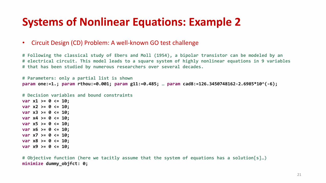
• Circuit Design (CD) Problem: A well-known GO test challenge

# Following the classical study of Ebers and Moll (1954), a bipolar transistor can be modeled by an # electrical circuit. This model leads to a square system of highly nonlinear equations in 9 variables # that has been studied by numerous researchers over several decades.

# Parameters: only a partial list is shown param one:=1.; param rthou:=0.001; param g11:=0.485; … param cad8:=126.3450748162-2.6985*10^(-6);

# Decision variables and bound constraintsvar x1 >= 0 <= 10;var x2 >= 0 <= 10; var x3 >= 0 <= 10;var x4 >= 0 <= 10; var x5 >= 0 <= 10;var x6 >= 0 <= 10; var x7 >= 0 <= 10;var x8 >= 0 <= 10; var x9 >= 0 <= 10;

# Objective function (here we tacitly assume that the system of equations has a solution[s]…)minimize dummy_objfct: 0;


21

# Constraints (all constraints are nonlinear)

subject to

con1 : (one-x1*x2)*x3*(exp(x5*(g11-g31*x7*rthou-g51*x8*rthou))-one)-g51+g41*x2+cad1 = 0;




con5 : (one-x1*x2)*x4*(exp(x6*(g11-g21-g31*x7*rthou+g41*x9*rthou))-one)-g51+g41*x2+cad5 = 0;




con9 : x1*x3-x2*x4 = 0;


22

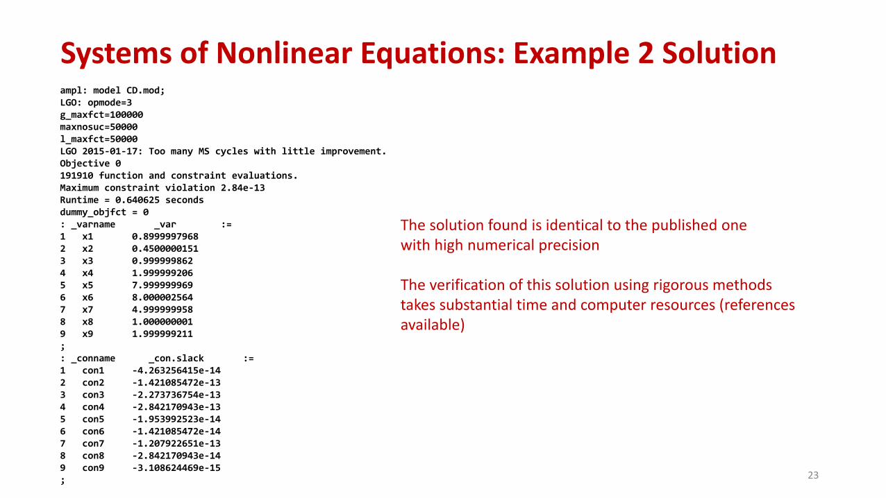
ampl: model CD.mod; LGO: opmode=3g_maxfct=100000maxnosuc=50000l_maxfct=50000LGO 2015-01-17: Too many MS cycles with little improvement.Objective 0191910 function and constraint evaluations.Maximum constraint violation 2.84e-13Runtime = 0.640625 secondsdummy_objfct = 0: _varname _var :=1 x1 0.89999979682 x2 0.45000001513 x3 0.9999998624 x4 1.9999992065 x5 7.9999999696 x6 8.0000025647 x7 4.9999999588 x8 1.0000000019 x9 1.999999211;: _conname _con.slack :=1 con1 -4.263256415e-142 con2 -1.421085472e-133 con3 -2.273736754e-134 con4 -2.842170943e-135 con5 -1.953992523e-146 con6 -1.421085472e-147 con7 -1.207922651e-138 con8 -2.842170943e-149 con9 -3.108624469e-15;

Systems of Nonlinear Equations: Example 2 Solution

23

The solution found is identical to the published one with high numerical precision

The verification of this solution using rigorous methods takes substantial time and computer resources (references available)

1 2 3 4 5 6

-2

-1

1

2

3

Globally optimized model fit, data with random noise (Cited from JDP, Opt. Methods and Software, 2003)

An example developed in Mathematica: a + Sin[b*(Pi*t) + c] + Cos[d*(3Pi*t) + e] + Sin[f*(5Pi*t) + g] +

Globally Optimized Model Fitting to Data

24

Model Calibration in AMPL: An Example 1

25

# Problem statement: Given the input data vector x[K] and output data vector y[K]), find the optimized # parameters of a postulated model type (structure), by minimizing the least squares error between # model output and observations.

# To run this model, enter in the command window# model MC.mod;

# reset AMPLreset;

# Number of data points (time steps) in this exampleparam Tmax := 250;set T = 1..Tmax;

# Equidistant input valuesparam x{T};let {t in T} x[t] := t/Tmax;

# Preset optimal parameter values param a0 := 1;param b0 := 2;param c0 := 3;param d0 := 4;param e0 := 5;


26

# Noise term standard deviation parameter used in normal distribution based model Normal(0, stdev);param stdev = 0.1;# To guarantee reproducible (identical) run results, set random seed parameter to a fixed valueoption randseed 1;

# Calculated model output values param y{T};

# Assign data set based on a postulated nonlinear model + noise termlet {t in T} y[t] := (x[t] - c0)^2 + (x[t] - d0)^2 + (x[t] - e0)^2 + sqrt(a0 + e0*x[t]) + 7*cos(3*b0*x[t] + c0) - 12*sin(2*a0*x[t]+c0) + log(1 + a0*x[t]) + Normal(0,stdev);

# Decision variables to optimizevar a >= 0 <= 6;var b >= 0 <= 6;var c >= 0 <= 6;var d >= 0 <= 6;var e >= 0 <= 6;

# Least squares error objectiveminimize LSError: sum {t in T} (y[t] - ((x[t] - c)^2 + (x[t] - d)^2 +(x[t] - e)^2 + sqrt(a + e*x[t]) + 7*cos(3*b*x[t] + c) - 12*sin(2*a*x[t]+c) + log(1 + a*x[t])))^2;


27

option solver lgo; option lgo_options 'g_maxfct = 100000 maxnosuc = 100000 l_maxfct = 100000’;

solve;

display sqrt(LSError)/Tmax;display _varname, _var; display sqrt(LSError)/Tmax > MC.txt;display _varname, _var >> MC.txt;

# Result obtained (retrieved from MC.txt file) # Recalling the noise model, the solution (1, 2, 3, 4, 5) can be recovered only approximately

sqrt(LSError)/Tmax = 0.006486728897

: _varname _var :=1 a 1.0026296442 b 1.9951451433 c 3.0043398884 d 3.9567559915 e 5.024104229;

Optimized Calibration of Artificial Neural Networks

For concise ANN background, consult, e.g, https://en.wikipedia.org/wiki/Artificial_neural_network

Image from https://www.analyticsvidhya.com/blog/2016/08/evolution-core-concepts-deep-learning-neural-networks/

28Globally optimized ANN model parameters: cf. JDP, Expert Systems with Applications, 2012

Data Classification (Clustering) by Global Optimization

• Objective: find the most homogeneous grouping of a given data set (black dots in the lhs figure).This can be done numerically, by globally optimizing the position of assigned cluster centers (medoids) ck k = 1…,K: see the red dots in the rhs figure. For an arbitrary candidate medoid configuration, one can use the nearest neighbor rule to assign the data to the cluster centers ck. DC quality is defined as the sum of all distances between the data and the associated ck.

• Example: 400 three-dimensional points classified into 4 clusters; GO is key to success… Consult JDP, Global Optimization in Action, Kluwer AP / Springer, 1996

→

29

Mathematica + LGO used

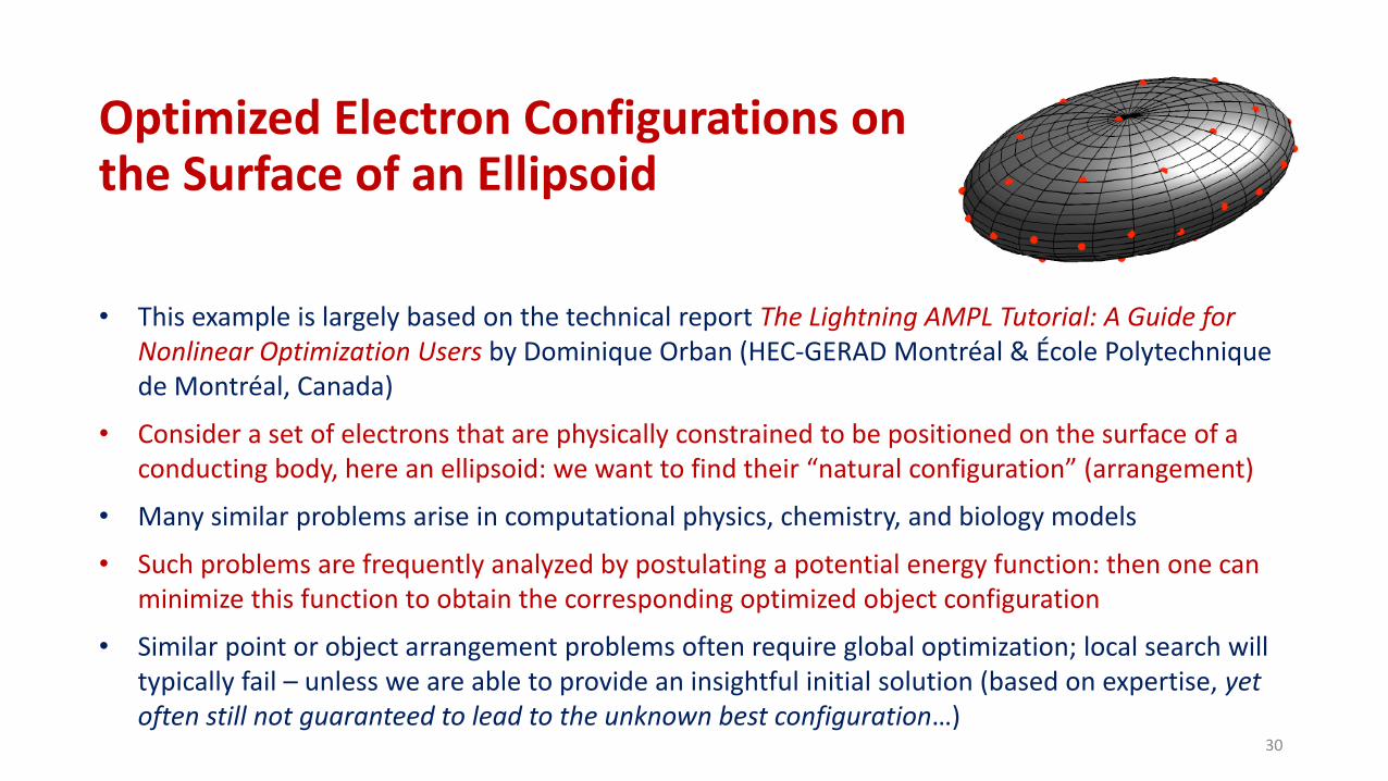
Optimized Electron Configurations on the Surface of an Ellipsoid

• This example is largely based on the technical report The Lightning AMPL Tutorial: A Guide for Nonlinear Optimization Users by Dominique Orban (HEC-GERAD Montréal & École Polytechnique de Montréal, Canada)

• Consider a set of electrons that are physically constrained to be positioned on the surface of a conducting body, here an ellipsoid: we want to find their “natural configuration” (arrangement)

• Many similar problems arise in computational physics, chemistry, and biology models

• Such problems are frequently analyzed by postulating a potential energy function: then one can minimize this function to obtain the corresponding optimized object configuration

• Similar point or object arrangement problems often require global optimization; local search will typically fail – unless we are able to provide an insightful initial solution (based on expertise, yet often still not guaranteed to lead to the unknown best configuration…)

30

Electrons on an Ellipsoid: Model Development

• We assume that the ellipsoid center is at the origin 0R3; the ellipsoid is defined by its half-axes rx, ry and rz: these are model parameters

• This is a scalable model: the number N of electrons can be chosen as a model parameter

• Decision variables are the electron positions (x[i], y[i], z[i]) for i = 1..N

• Constraints express the fact that all electrons must be located on the ellipsoid surface:

(x[i]/rx)2 + (y[i]/ry)2 + (z[i]/rz)2 = 1 Here x[i] corresponds to xi, and so on: see function U(.) below

• Objective: The potential energy function used here is the Coulomb potential U(.), defined by the sum of reciprocal pairwise distances of all electrons as follows (ignoring a physical constant) :

31

AMPL Model File

model; # Opens up a model file: this command has to be in the model file or in the call

param N > 0, integer ; # Number of electrons: its value will be defined in the data file

param rx > 0; # Half axis of ellipse in direction x: value is given in the data file

param ry > 0; # Half axis of ellipse in direction y: value is given in the data file

param rz > 0; # Half axis of ellipse in direction z: value is given in the data file

var x {1..N} >=-rx <= rx; # x-coordinates of the electrons, with tight bounds

var y {1..N} >=-ry <= ry; # y-coordinates of the electrons, with tight bounds

var z {1..N} >=-rz <= rz; # z-coordinates of the electrons, with tight bounds

minimize CoulombPotential : # Objective function

sum {i in 1..N-1} sum {j in i+1..N} 1/sqrt ( (x[i]-x[j ])^2 + (y[i]-y[j ])^2 + (z[i]-z[j ])^2 );

subject to # All electrons are located on the surface of the ellipsoid

EllipsoidConstraint {i in 1..N}: x[i ]^2 /rx ^2 + y[i ]^2 /ry ^2 + z[i ]^2 /rz ^2 = 1;

# RangeConstraint {i in 1..N}: -0.5*rz <= z[i] <= 0.5*rz; # An example of optional tighter bounds

32

Optimized Object Packings: Further Examples

33

Optimized Circle Packing for n=25

Embedding circle contains circles with radii rk =k-0.5 k=1,…,25

• General problem: given a set of objects, find a given type of container with minimal size which contains all these objects in a non-overlapping arrangement

• In practice, further criteria (e.g., balance conditions) need to be also considered

Credits: Collaboration with Frank Kampas, Ignacio Castillo, Giorgio Fasano, Tatiana Romanova et al.; articles and book chapters available

Optimized Object Packings: Further Examples

34Credits: Collaboration with Ignacio Castillo and Frank Kampas

“Black Box” Optimization 1

35

• Motivation: I have been working for a long time as an independent researcher / software developer / consultant / lecturer and trainer

• Interdisciplinary research often leads to “black box” nonlinear optimization

• The person(s) in charge of optimization don’t necessarily have access to the descriptive models with parameters to optimize… certain details and model properties may be unknown

Some application areas based on my own work experience (list continued on next two slides)

• advanced engineering design (acoustics, automotive, lasers, optics, and other areas)

• biotechnology

• chemical process analysis

• computational physics and chemistry


36

Application areas (continued)

• defence

• environmental systems analysis and management

• financial modeling and optimization

• industrial product design

• model calibration

• oil and gas production

• process control

• radiation therapy planning

• risk analysis and management


37

Application areas (continued)

• robot equipment design

• scientific modelling

• space engineering

and many other areas…

• Credits: Collaboration with Roger Cooke, Mustafa Çaĝlayan, Larry Deschaine et al., Giorgio Fasanoet al., Mark Gammon et al., Zoltán Horváth et al., Glenn Isenor, Thomas Mason et al., Maplesoft’s engineering application development team, Grigoris Pantoleontos et al., Christopher Purcell et al., Jouko Tervo et al., and a large number of other colleagues

• Related publications are available upon request;

• To illustrate, here two “black box” optimization applications are highlighted

“Black Box” Optimization: Intensity Modulated Radiotherapy

38

Descriptive model development by Jouko Tervo et al., U. of Kuopio

Objective: targeted dose to treatedregion, while – ideally – minimal radiation to surrounding tissue and organs at risk

See illustrative figure that shows globally optimized dose distribution; much better than earlier locally optimized dose distribution plans

Joint article and book chapter available

“Black Box” Optimization: Suspension System Design

• This case study was developed in collaboration with Maplesoft

• Goal: Given a required (target) behavior of a double wishbone suspension system – defined in terms of the displacement curves for bumps on the road – we want to find its optimal design point settings, known as “hard points”, that result in an optimized smooth ride

• “Black box” descriptive model: DynaFlex Pro software by MotionPro used to model this system; the resulting inverse problem is then solved by the Global Optimization Toolbox (LGO linked to Maple)

• Citing the application director of Maplesoft at the time of this study, global optimization helped to find a “stunning design”…

39

Concluding Notes

• Facing the vast universe of nonlinear systems and processes, we have an unlimited source of important, motivating (and often hard) modeling and optimization problems

• Frequently, interdisciplinary research is required

• The future of creative thinking – integrating concepts and tools from business analytics, operations research, systems engineering, and computational optimization – is bright!

• Continuing expansion of examples collected to teach optimization: new models welcome!

• Interested in collaborative R&D, training and consulting opportunities

• Articles and further information are available upon request

• Current (Lehigh University) personal webpage, with a professional summary and links to books https://engineering.lehigh.edu/faculty/janos-d-pinter

• Google Scholar http://scholar.google.ca/citations?user=iHrfmDEAAAAJ&hl=en&oi=ao40

https://engineering.lehigh.edu/faculty/janos-d-pinter

http://scholar.google.ca/citations?user=iHrfmDEAAAAJ&hl=en&oi=ao

Illustrative References 1

JDP: Global Optimization, LGO Software Versions, Benchmarking

41

• Global Optimization in Action. Kluwer Academic Publishers, Dordrecht, 1996.

• Computational Global Optimization in Nonlinear Systems – An Interactive Tutorial. Lionheart Publishing, Atlanta, GA, 2001.

• Global optimization: software, test problems, and applications, in Pardalos, P.M. and Romeijn, H.E., Eds.Handbook of Global Optimization, Volume 2, pp. 515-569. Kluwer Academic Publishers, Dordrecht, 2002.

• Software development for global optimization, in: Pardalos, P.M. and T. F. Coleman, Eds. Global Optimization: Methods and Applications, pp. 183-204. American Mathematical Society, Providence, RI, 2009.

• Benchmarking nonlinear optimization software in technical computing environments. TOP 21 (2013), 33-162. (Joint work with F.J. Kampas)

• LGO Solver Suite for Global and Local Nonlinear Optimization: User's Guide. PCS Inc., 2017.

• How difficult is nonlinear optimization? A practical solver tuning approach, with illustrative results. Annals of Operations Research 265 (2018), pp. 119–141.


Edited Books on NLP and GO Applications

42

• JDP, Ed., Global Optimization: Scientific and Engineering Case Studies. Springer Science + Business Media, New York, 2006.

• Fasano, G. and JDP, Eds., Modeling and Optimization in Space Engineering. Springer Science + Business Media, New York, 2013.

• Fasano, G. and JDP, Eds., Optimized Packings With Applications. Springer Science + Business Media, New York, 2015.

• Fasano, G. and JDP, Eds., Space Engineering: Modeling and Optimization with Case Studies. Springer Science + Business Media, New York, 2016.

• Fasano, G. and JDP, Eds., Modeling and Optimization in Space Engineering: State of the Art and New Challenges. Springer Science + Business Media, New York, 2019.


Some Challenging Global Optimization Applications

43

• JDP, Globally optimized calibration of environmental models. Annals of Operations Research 25 (1990) 211-222.

• JDP, Stochastic modelling and optimization for environmental management. Annals of Operations Research 31 (1991) 527-544.

• Tervo, J., Kolmonen, P., JDP, Lyyra-Laitinen, T., and Lahtinen, T., An optimization-based approach to the multiple static delivery technique in radiation therapy. Annals of Operations Research 119 (2003) 205-227.

• Isenor, G., JDP, Cada, M., A global optimization approach to laser design. Optimization and Engineering 4 (2003) (3) 177-196.

• Castillo, I., JDP, Lee, T., Integrated software tools for the OR/MS classroom. Algorithmic Operations Research 3 (2008) 82–91.

• I., Castillo, F.J. Kampas, JDP, Solving circle packing problems by global optimization: numerical results and industrial applications. European Journal of Operational Research 191 (2008) 786–802.


Further Challenging Global Optimization Applications

44

• Pantoleontos, G., Basinas, P. Skodras, G., Grammelis, JDP, P. Topis, S., Sakellaropoulos, G.P., A global optimization study on the devolatilisation kinetics of coal, biomass and waste fuels. Fuel Processing Technology 90 (2009) 762-769.

• JDP, Calibrating artificial neural networks by global optimization, Expert Systems with Applications 39 (2012) 25–32.

• Çaĝlayan, M.O., JDP, Development and calibration of currency market strategies by global optimization. Journal of Global Optimization 56 (2013), 353-371.

• JDP, Horváth, Z., Integrated experimental design and nonlinear optimization to handle computationally expensive models under resource constraints. Journal of Global Optimization 57 (2013) 191-215.

• Deschaine, L.M. Lillys, T.P., JDP, Groundwater remediation design using physics-based flow, transport, and optimization technologies. Environmental Systems Research 2 (2013) 2:6.

• JDP, F.J. Kampas, and I. Castillo, Globally optimized packings of non-uniform size spheres in Rd: A computational study, Optimization Letters 12 (2018) 3, pp. 585–613.

• Yu. Stoyan, A. Pankratov, T. Romanova, G. Fasano, JDP, Yu. Stoian, A. Chugay, Optimized packings in space engineering applications: Part I. In: Fasano and JDP, Eds., (2019): see slide on edited volumes

Thanks for your attention!

Questions and comments [email protected]

45

Documents

Nonlinear Optimization in AMPL with LGO