Nonlinear Dynamics of Electrostatic Comb-drivewith Variable Gap Under Harmonic ExcitationAlexey V. Lukin ( lukinalexei@yandex.ru )

Peter the Great Saint Petersburg Polytechnic University: Sankt-Peterburgskij politehniceskij universitetPetra Velikogo https://orcid.org/0000-0003-2016-8612Dmitry Indeitsev

Peter the Great Saint Petersburg Polytechnic University: Sankt-Peterburgskij politehniceskij universitetPetra VelikogoIvan Popov

Peter the Great Saint Petersburg Polytechnic University: Sankt-Peterburgskij politehniceskij universitetPetra VelikogoNadezhda Mozhgova

Peter the Great Saint Petersburg Polytechnic University: Sankt-Peterburgskij politehniceskij universitetPetra Velikogo

Research Article

Keywords: Electrostatic comb-drive, elastic suspension, vibration amplitude.

Posted Date: September 14th, 2021

DOI: https://doi.org/10.21203/rs.3.rs-873502/v1

License: This work is licensed under a Creative Commons Attribution 4.0 International License. Read Full License

Nonlinear dynamics of electrostatic comb-drive

with variable gap under harmonic excitation

N. V. Mozhgova1, A. V. Lukin*1, I. A. Popov1, and D. A.Indeitsev1,2

1Peter the Great St.Petersburg Polytechnic University, SaintPeterburg, Russia

2Institute for Problems in Mechanical Engineering of the RussianAcademy of Sciences, Saint Peterburg, Russia

September 2, 2021

Contents

1 Introduction 2

2 Mathematical model 42.1 Transformation of the equation of motion for the application of

MSM . . . . . . . . . . . . . . . . . . . . . . . . . . . . . . . . . . 62.1.1 Dynamics equation: multiplication by the denominator . 72.1.2 Dynamics equation: Taylor series expansion . . . . . . . . 8

3 Multiple scales method 93.1 Multiplication equation by the denomanator of right-hand side . 93.2 Taylor series expansion for the electrostatic force . . . . . . . . . 12

4 Results 134.1 Validation of equation systems in slow variables . . . . . . . . . . 134.2 Static Equilibrium Diagrams and Static Displacement Function

Approximation . . . . . . . . . . . . . . . . . . . . . . . . . . . . 174.3 Analysis of the amplitude-frequency response of the system . . . 214.4 Analysis of the amplitude-force response of the system . . . . . . 264.5 Continuation of the resonant-mode solution . . . . . . . . . . . . 28

4.5.1 Resonant regime dependence on VAC . . . . . . . . . . . . 294.5.2 Resonant regime dependence on VDC . . . . . . . . . . . . 32

5 Conclusion 35

*Corresponding author. E-mail: lukinalexei@yandex.ru

6 Funding 35

7 Conflict of Interest 35

8 References 36

Abstract

This paper provides an extensive study of the nonlinear dynamics

of a variable gap electrostatic comb-drive. The amplitude- and phase-

frequency response, as well as the amplitude- and phase-force response of

the comb-drive were obtained and analyzed with and without taking into

account the cubic nonlinearity of the suspension. A significant variation

in the frequency and force response is demonstrated in the presence of

nonlinearity of the elastic suspension. Using numerical methods of bi-

furcation theory, solutions are obtained that correspond to the resonance

peak of the frequency response when the constant and variable compo-

nents of the voltages change. The result obtained makes it possible to

determine the range of excitation voltage values that provide the required

vibration amplitude in the resonant mode. The influence of the second

stationary electrode on the dynamics of the system is estimated. The

significant influence of this factor on the resonant-mode characteristics is

revealed.

1 Introduction

The development of nano- and microsystem technology (NMST or, inother words, nano- and micro-electromechanical systems – NEMS / MEMS) wasinitially closely associated with the development of semiconductor technologies.From a manufacturing point of view, the very fabrication technology based onselective etching/deposition of silicon has evolved along with semiconductorssince the 1950s, but the use of such technologies for the manufacture of micro-scale devices with moving sensing elements – MEMS sensors – did not beginuntil the mid-1970s. – 1980s [Iannacci]. Manufacturing techniques that useanisotropic etching to produce various three-dimensional suspended structuresfrom a silicon substrate have led to the implementation of miniature pressuresensors, accelerometers, gyroscopes, switches and other devices for various ap-plications, for example, in the optical and biomedical fields. A further impetusin the development of microsystem technology is associated with the improve-ment of surface micromachining technology and today MEMS technologies areused in all spheres of human life from rocketry to inkjet printing technologies[Varadan, Raspopov].

Any MEMS sensor includes a sensing element, a system of elastic sus-pensions to ensure the mobility of the sensing element, as well as a system forexciting oscillations and picking up a signal by electrostatic, piezoelectric, mag-netic or thermal interactions. Electrostatic excitation is the most commonlyused method because it is easy to implement and compatible with Complemen-tary metal–oxide–semiconductor (CMOS) circuits. This type of actuation of a

2

micro-electromechanical system is based on the attractive force between plateswith different electric charges and can be divided into two subtypes – movementperpendicular (variable gap) and parallel (variable area) to the electrode plane[Acar]. The advantage of variable gap drives over variable area ones lies inthe magnitude of the generated electrostatic force – when the gap changes, it ismuch greater. However, the disadvantage of such a system is the restriction onthe displacement of the movable electrode – when the displacement exceeds onethird of the interelectrode gap, the electrodes collapse, and the system fails.

When modeling drives with variable gap, due to the nonlinearity of thedependence of the electrostatic force on the displacement of the moving electrode[Acar], it is necessary to use asymptotic methods and conduct a qualitativeanalysis of the system behavior.

When investigating the nonlinear dynamics of a variable gap electro-static drive, the mathematical model usually takes into account the cubic non-linearity of the elastic suspension [Zhang1, Ilyas, Rhoads, Hajjaj, Han]and the viscous friction (Squeeze Film Damping) [Zhang1]. For the analysis,asymptotic methods of nonlinear dynamics are used, in particular, the multiplescales method [Zhang1, Ilyas, Hajjaj, Han]. The expansion of the expressionfor the electrostatic force in the Taylor series is also used [Zhang1]. Sometimesfor a more precise description, the expansion in the Taylor series is avoided byusing the averaging theorem together with the residue theorem to obtain anapproximate analytical solution [Zhang2].

As a result of the application of the above methods, it becomes possibleto obtain and then analyze the amplitude-frequency response (AFR) of the sys-tem when considering the main and/or subharmonic resonances. For example,[Zhang1] describes the influence of the parameters of the constant and variablevoltage components on the character of the frequency response and the value ofnatural frequencies.

An electrostatic drive with a variable gap can be used not only as aexcitation system of the device. For example, [Shkel] demonstrates the effectof amplitude modulation on the Q-factor and noise level in the output of a mi-cromechanical gyroscope. Electrothermal modulation allows you to separate theuseful signal from the parasitic ones in the frequency domain. It is shown thatthe carrier signal of an alternating current is an accurate method for adjust-ing the Q-factor of an micromechanical gyroscope, and it is also demonstratedthat with the correct setting of the parameters, the signal-to-noise ratio can beimproved by a factor of 6.

The work [Pistorio] proposes a model of an LL-type dual mass gyro-scope, in which the drive system is an electrostatic actuator with a variable area,but a variable gap drive has also found its application – it is used to adjust theresonant frequency along the sensitivity axis closer to the midrange along driveaxis to provide the desired difference between them with temperature interfer-ence and manufacturing errors.

The purpose of this work is to study the nonlinear dynamics of an elec-trostatic comb drive with a variable gap to establish the dependence of theoscillation amplitude of the moving electrode on the constant and variable volt-

3

age components, taking into account the specified geometric and mass-inertialcharacteristics.

Relevance of the work is due to the intensive development of nano- andmicrosystem technology, leading to the development and manufacture of newand more complex micromechanical sensors for various purposes, requiring theconstruction and study of mathematical models of MEMS elements, includingelectrostatic actuators [Hajjaj]. In particular, there is a need for an accurateassessment of the comb-drive excitation voltages values, depending on electrome-chanical characteristics of the device, at the stage of it’s initial design (namely,micromechanical vibration gyroscopes and resonant, as well as mode-localized,accelerometers) [Zotov, Lukin, Lukin2]

The novelty of the work lies in a detailed qualitative study of resonantoperating mode of an electrostatic drive with a variable gap, including takinginto account the second stationary electrode, which requires the joint finding ofsolutions to both the problem of nonlinear statics and nonlinear dynamics of amoving mass.

The work is divided into four sections. A mathematical model andtransformation of equations for further application of asymptotic methods ofnonlinear dynamics are given in Section 2. Further, in Section 3, systems ofequations in slow variables obtained after applying the multiple scales methodare presented. Finally, Section 4 is a presentation and analysis of the resultsobtained.

2 Mathematical model

A model of an electrostatic drive with a variable gap, consisting of amovable and two stationary electrodes with a gaps d1 and d2 between them,shown in the figure 1, is considered.

4

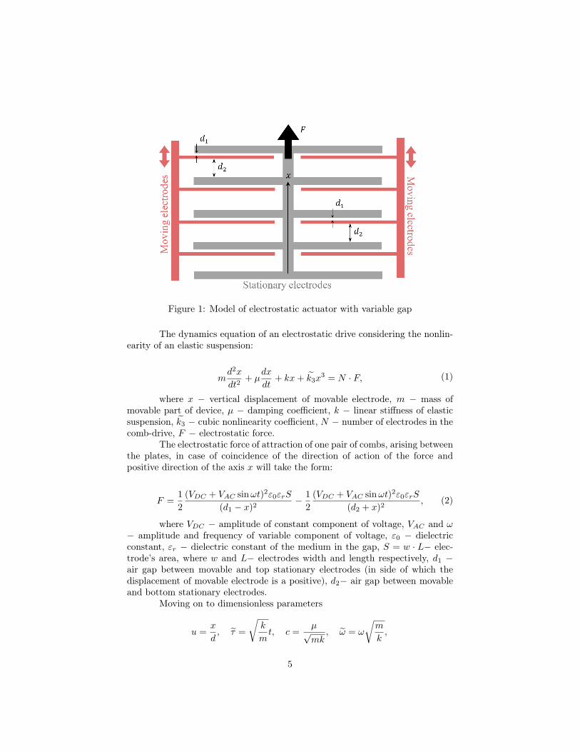
Figure 1: Model of electrostatic actuator with variable gap

The dynamics equation of an electrostatic drive considering the nonlin-earity of an elastic suspension:

md2x

dt2+ µ

dx

dt+ kx+ k3x

3 = N · F, (1)

where x − vertical displacement of movable electrode, m − mass ofmovable part of device, µ − damping coefficient, k − linear stiffness of elasticsuspension, k3 − cubic nonlinearity coefficient, N − number of electrodes in thecomb-drive, F − electrostatic force.

The electrostatic force of attraction of one pair of combs, arising betweenthe plates, in case of coincidence of the direction of action of the force andpositive direction of the axis x will take the form:

F =1

2

(VDC + VAC sinωt)2ε0εrS

(d1 − x)2− 1

2

(VDC + VAC sinωt)2ε0εrS

(d2 + x)2, (2)

where VDC − amplitude of constant component of voltage, VAC and ω− amplitude and frequency of variable component of voltage, ε0 − dielectricconstant, εr − dielectric constant of the medium in the gap, S = w · L− elec-trode’s area, where w and L− electrodes width and length respectively, d1 −air gap between movable and top stationary electrodes (in side of which thedisplacement of movable electrode is a positive), d2− air gap between movableand bottom stationary electrodes.

Moving on to dimensionless parameters

u =x

d, τ =

√k

mt, c =

µ√mk

, ω = ω

√m

k,

5

λ =1

2

ε0εrS(V2DC + 1

2V 2AC)

kd3, λ1 =

ε0εrSVACVDC

kd3,

λ2 =1

4

ε0εrSV2AC

kd3, k3 =

k3d2

k, p =

d2d1

,

the equation of motion is transformed to the form

d2u

dτ2+ c

du

dτ+ u+ k3u

3 =λ

(1− u)2− λ

(p+ u)2+

λ1 sin ωτ

(1− u)2−

− λ1 sin ωτ

(p+ u)2− λ2 cos 2ωτ

(1− u)2+

λ2 cos 2ωτ

(p+ u)2.

(3)

Unknown function of displacement u(τ) is decomposed into static dis-placement of the electrode u0 under the action of time-independent componentsof electrostatic force and a dynamic time-dependent term ξ(τ):

u = u0 + ξ(τ).

The static displacement of the electrode is determined from the equationof static equilibrium:

u0 + k3u30 =

λ

(1− u0)2− λ

(p+ u0)2. (4)

As a result of substituting the expansion of the displacement functioninto the equation of motion, an equation for the dynamic term ξ(τ) will beobtained:

ξ + cξ + u0 + ξ + k3(u0 + ξ)3 =λ

(1− u0 − ξ)2− λ

(p+ u0 + ξ)2+

+λ1 sin ωτ

(1− u0 − ξ)2− λ1 sin ωτ

(p+ u0 + ξ)2− λ2 cos 2ωτ

(1− u0 − ξ)2+

λ2 cos 2ωτ

(p+ u0 + ξ)2,

(5)

where () − derivative with respect to dimensionless time ddτ

. Afterwardsit is necessary to exclude the static part (4) from this equation.

2.1 Transformation of the equation of motion for the ap-

plication of MSM

The resulting equation (5) is nonlinear and cannot be qualitatively in-vestigated without the use of asymptotic methods of nonlinear dynamics. Inthis work, the multiple-scale method (MSM) is used [Nayfeh], but to apply it,it’s necessary to transform the right-hand side of the equation so that it doesnot contain terms with an unknown function ξ(τ) in the denominator. In this

6

regard, further transformations of the resulting equation will be carried out intwo ways:1. multiplication of the whole equation by the denominator of right-hand side;2. expansion of a fraction in a Taylor series up to the third order.

Also, in addition to the complete formulation of the problem, a simplifiedone will be also considered – without taking into account the influence of thesecond stationary electrode.

The equation of static equilibrium in the absence of a second stationaryelectrode is:

u0 + k3u30 =

λ

(1− u0)2, (6)

and also the equation of motion (5):

ξ + cξ + u0 + ξ + k3(u0 + ξ)3 =λ

(1− u0 − ξ)2+

λ1 sin ωτ

(1− u0 − ξ)2− λ2 cos 2ωτ

(1− u0 − ξ)2,

(7)

Further, the equation (7) will be reduced to a more analytically conve-nient form for applying the MSM in two ways – by multiplying by the denomi-nator of the right-hand side and using the Taylor series expansion.

2.1.1 Dynamics equation: multiplication by the denominator

After multiplying the equation (7) by the denominator of the right-handside, it becomes:

((1− u0)2 − 2(1− u0)ξ + ξ2)(ξ + cξ + u0 + ξ + k3(u0 + ξ)3) =

λ+ λ1 sin ωτ − λ2 cos 2ωτ .(8)

From this equation it is necessary to exclude the terms representing theequation of static equilibrium (6). Also, for ease of use in the future of themultiple-scale method, another change of the time variable was made in orderto obtain the dimensionless frequency of the linear part of the equation, equalto unity:

Ω2 = 1 + 3u20k3 −

2k3u30

1− u0

− 2u0

1− u0

, τ = Ωτ , η =ω

Ω. (9)

After all the transformations and grouping of the terms of the equationby powers of ξ, the final equation of motion was obtained:

ξ + C1ξ + ξ − C2ξξ − C3ξξ + C4ξ2ξ + C5ξ

2ξ + C6ξ2 + C7ξ

3 + C8ξ4+

+C9ξ5 = C10λ1 sin ητ − C10λ2 cos 2ητ,

(10)

7

where the coefficients Ci, i = 1 : 10 are

C1 =c

Ω, C2 =

2

1− u0

, C3 =2c

(1− u0)Ω

C4 =1

(1− u0)2, C5 =

c

Ω(1− u0)2,

C6 = − 2

Ω2(1− u0)+

3k3u0

Ω2− 6k3u

20

Ω2(1− u0)+

k3u30

Ω2(1− u0)2+

u0

Ω2(1− u0)2,

C7 =k3Ω2

− 6k3u0

Ω2(1− u0)+

1

Ω2(1− u0)2+

3u20k3

Ω2(1− u0)2,

C8 = − 2k3Ω2(1− u0)

+3u0k3

Ω2(1− u0)2,

C9 =k3

Ω2(1− u0)2, C10 =

1

Ω2(1− u0)2.

2.1.2 Dynamics equation: Taylor series expansion

The expression for the electrostatic force in the absence of the influenceof the second stationary electrode has the form

F =1

(1− u0 − ξ)2(λ+ λ1 sin ωτ − λ2 cos 2ωτ). (11)

The factor in front of the bracket can be expanded into a Taylor seriesin function ξ at the point ξ0 = 0 up to the third order inclusive:

1

(1− u0 − ξ)2=

1

(1− u0)2+

2ξ

(1− u0)3+

3ξ2

(1− u0)4+

4ξ3

(1− u0)5+O(ξ4).

(12)

After substituting this expansion into the original equation (7) and ex-cluding the terms that make up the equation of static equilibrium (6), similarlyto the previous case, the time variable was also replaced:

Ω2 = 1 + 3u20k3 −

2λ

(1− u0)3, τ = Ωτ , η =

ω

Ω. (13)

After all the transformations and grouping of the terms of the equationby powers of ξ, the final equation of motion was obtained, suitable for applyingthe multiple-scale method

8

ξ + C1ξ + ξ − C2λ1 sin ητ + C2λ2 cos 2ητ + ξ2(C3 − C4λ1 sin ητ + C4λ2 cos 2ητ)+

+ξ3(C5 − C6λ1 sin ητ + C6λ2 cos 2ητ) = C7λ1 sin ητ − C7λ2 cos 2ητ,

(14)

where the coefficients Ci, i = 1 : 7 are

C1 =c

Ω, C2 =

2

Ω2(1− u0)3, C3 =

3k3u0

Ω2− 3λ

Ω2(1− u0)4

C4 =3

Ω2(1− u0)4, C5 =

k3Ω2

− 4λ

Ω2(1− u0)5,

C6 =2

Ω2(1− u0)5, C7 =

1

Ω2(1− u0)2.

Due to the fact that when the second fixed electrode is taken into ac-count, the right-hand side of the equation of motion contains several fractionswith two different denominators, in this problem only the method with theexpansion of the electrostatic force in the Taylor series will be considered.

The derivation of the equation of motion is similar to the derivation inthe absence of the second fixed electrode in the model. The equation of motionhas the form (14), and the dimensionless frequency after changing the timevariable, and the coefficients Ci, where i = 1 : 7, are

Ω = 1 + 3k3u20 −

2λ

(1− u0)3− 2λ

(p+ u0)3,

C1 =c

Ω, C2 =

2

Ω2(1− u0)3+

2

Ω2(p+ u0)3, C3 =

3k3u0

Ω2− 3λ

Ω2(1− u0)4+

3λ

Ω2(p+ u0)4

C4 =3

Ω2(1− u0)4− 3

Ω2(p+ u0)4, C5 =

k3Ω2

− 4λ

Ω2(1− u0)5− 4λ

Ω2(p+ u0)5,

C6 =4

Ω2(1− u0)5+

4

Ω2(p+ u0)5, C7 =

1

Ω2(1− u0)2− 1

Ω2(p+ u0)2.

3 Multiple scales method

3.1 Multiplication equation by the denomanator of right-

hand side

Terms in equation (10) are scaled as follows:

ξ + ε2C1ξ + ξ − C2ξξ − εC3ξξ + C4ξ2ξ + C5ξ

2ξ + C6ξ2 + C7ξ

3 + C8ξ4+

+ C9ξ5 = ε3C10λ1 sin ητ − εC10λ2 cos 2ητ,

(15)

9

where ε − small parameter.The multi-scale decomposition [Nayfeh] will be performed up to third

order inclusive. Therefore, before the main member of electrostatic force (whenconsidering the main resonance) there is a small parameter in third degree. Alsoterms with the first time derivative ξ fall into the third order of decomposition.The double-frequency term of electrostatic force must fall into the first-ordersolution, so a small parameter is also added before it.

A three-term expansion is considered in the form

ξ(τ, ε) = εξ1(T0, T1, T2) + ε2ξ2(T0, T1, T2) + ε3ξ3(T0, T1, T2), (16)

where Tn = εnτ .Time derivatives are defined as:

d

dτ= D0 + εD1 + ε2D2, Dn =

∂

∂Tn

.

After substituting the expansion (16) into the equation (15) and bal-ancing in powers of a small parameter, the following expressions were obtained:

O(ε1) : D20ξ1 + ξ1 = C10λ2 cos 2ητ =⇒ A exp(iωT0) + Λ exp(2iωT0) + cc,

(17)

where Λ = C10λ2

1−4η2 , A = A(T1, T2) = 1

2a expiβ, where a and β− slow

amplitude and phase, and cc − complex conjugate members.

O(ε2) : D20ξ2 + ξ2 = −2D0D1ξ1 + C2D

20ξ1ξ1 − C6ξ

21 − C5D0ξ1ξ

21 + cc, (18)

O(ε3) : D20ξ3 + ξ3 = −2D0D1ξ2 − 2D0D2ξ1 −D2

1ξ1+

+C2D20ξ1ξ2 − C1D0ξ1 + C2D

20ξ2ξ1 + 2C2D0D1ξ1ξ1 + C3D0ξ1ξ1−

−C4D20ξ1ξ

21 − C5D0ξ2ξ

21 − C5D1ξ1ξ

21 − 2C5D0ξ1ξ1ξ2 − C7ξ

31 − 2C6ξ1ξ2+

+C10λ1 sin ηT0.

(19)

The main resonance is subject to consideration, so

η = 1 + εσ. (20)

After carrying out the further procedure of the MSM, a system of equa-tions in slow variables was obtained

10

a′ =2C2C10λ2

3 (4η2 − 1)a cos(2γ)− 1

8C5a

3 − 1

2C10λ1 cos(γ)−

C5C102λ2

2

4(4η2 − 1)2a− 1

2C1a−

− C3C10λ2

4 (4η2 − 1)a cos(2γ) +

2C6C10λ2

3 (4η2 − 1)a cos(2γ)− 5C2C10λ2

4 (4η2 − 1)a sin(2γ)−

− C6C10λ2

2 (4η2 − 1)a sin(2γ)− C2C10λ2σ

2

4η2 − 1a sin(2γ) +

2C2C10λ2σ

3 (4η2 − 1)a cos(2γ)−

− C3C10λ2σ

2 (4η2 − 1)a cos(2γ) +

2C6C10λ2σ

3 (4η2 − 1)a cos(2γ)− 2C2C10λ2σ

4η2 − 1a sin(2γ),

(21)

γ′ = −σ − 1

48a(2C2

2a3 + 20C2

6a3 + 18C4a

3 − 18C7a3 + 22C2C6a

3−

−24C10λ1 sin(γ) +108C4C10

2λ2

2

a

(4η2 − 1)2

− 36C7C102λ2

2

a

(4η2 − 1)2

− 273C22C10

2λ2

2

a

4(4η2 − 1)2

+

+15C2

6C102λ2

2

a

(4η2 − 1)2

− 180C22C10

2λ2

2

σa

(4η2 − 1)2

+96C4C10

2λ2

2

σ2a

(4η2 − 1)2

+

+60C2C10λ2 cos(2γ)a

4η2 − 1+

24C6C10λ2 cos(2γ)a

4η2 − 1+

32C2C10λ2 sin(2γ)a

4η2 − 1−

−12C3C10λ2 sin(2γ)a

4η2 − 1+

32C6C10λ2 sin(2γ)a

4η2 − 1− 234C2

2C102λ2

2

σ2a

(4η2 − 1)2

−

−144C22C10

2λ2

2

σ3a

(4η2 − 1)2

− 36C22C10

2λ2

2

σ4a

(4η2 − 1)2

+39C2C6C10

2λ2

2

a

(4η2 − 1)2

+

+192C4C10

2λ2

2

σa

(4η2 − 1)2

+48C2C10λ2σ

2 cos(2γ)a

4η2 − 1+

120C2C6C102λ2

2

σa

(4η2 − 1)2

+

+60C2C6C10

2λ2

2

σ2a

(4η2 − 1)2

+96C2C10λ2σ cos(2γ)a

4η2 − 1+

32C2C10λ2σ sin(2γ)a

4η2 − 1−

−24C3C10λ2σ sin(2γ)a

4η2 − 1+

32C6C10λ2σ sin(2γ)a

4η2 − 1),

(22)

where a and γ − dimensionless amplitude and phase, γ = β − τσ, σ−frequency offset parameter, which is determined by formula (20) for ε = 1, ()′−derivative with respect to dimensionless time.

The established solution is then sought from the conditions a′ = 0 andγ′ = 0. Substituting them into equations (21) and (22), a system of algebraicequations is obtained, the solutions of which are stationary amplitude and rel-ative phase of oscillations.

11

3.2 Taylor series expansion for the electrostatic force

Terms in equation (14) are scaled as follows:

ξ + ε2C1ξ + ξ − ε2C2λ1 sin ητ + ε2C2λ2 cos 2ητ+

+ξ2(C3 − εC4λ1 sin ητ + εC4λ2 cos 2ητ) + ξ3(C5 − C6λ1 sin ητ + C6λ2 cos 2ητ) =

= ε3C7λ1 sin ητ − εC7λ2 cos 2ητ.

(23)

After substituting the expansion (16) into the equation (23) and bal-ancing in powers of a small parameter, the following expressions were obtained:

O(ε1) : D20ξ1 + ξ1 = C7λ2 cos 2ητ =⇒ A exp(iωT0) + Λ exp(2iωT0) + cc, (24)

where Λ = C7λ2

1−4η2 .

O(ε2) : D20ξ2 + ξ2 = −2D0D1ξ1 − C3ξ

21 + cc, (25)

O(ε3) : D20ξ3 + ξ3 = −2D0D1ξ2 − 2D0D2ξ1 −D2

1ξ1 −D0ξ1C1−−C5ξ

31 − 2C3ξ1ξ2 + λ1 sin(ητ)(C7 + C2ξ1 + C4ξ

21 + C6ξ

31)−

−λ2 cos(2ητ)(C2ξ1 + C4ξ21 + C6ξ

31).

(26)

After carrying out the further procedure of the MSM, a system of equa-tions in slow variables was obtained

a′ =1

8C6λ2a

3 sin (2γ)− 1

2C7λ1 cos (γ)−

1

2C1a− 1

8C4λ1a

2 cos (γ)+

+1

4C2λ2a sin (2γ) +

9C6C72λ2

3

16(4η2 − 1)2a sin (2γ)− C4C7

2λ1λ2

2

4(4η2 − 1)2cos (γ)−

−3C6C73λ1λ2

3

16(4η2 − 1)3cos (γ) +

2C3C7λ2

3 (4η2 − 1)a cos (2γ)− C3C7λ2

2 (4η2 − 1)a sin (2γ)−

− C2C7λ1λ2

4 (4η2 − 1)cos (γ) +

3C6C7λ1λ2

16 (4η2 − 1)a2 cos (3γ)−

− 3C6C7λ1λ2

16 (4η2 − 1)a2 cos (γ) +

2C3C7λ2σ

3 (4η2 − 1)a cos (2γ) ,

(27)

12

γ′ =1

24a

[9C5a

3 − 10C23a

3 + 12C7λ1 sin(γ) + 6C6λ2a3 cos(2γ)+

+6C2λ2a cos(2γ) + 9C4λ1a2 sin(γ)− 12C4C7λ2

2

4η2 − 1a+

18C5C72λ2

2

(4η2 − 1)2a−

−15C23C7

2λ2

2

2(4η2 − 1)2a+

27C6C72λ2

3

2(4η2 − 1)2a cos(2γ)− 12C3C7λ2

4η2 − 1a cos(2γ)+

+6C4C7

2λ1λ2

2

(4η2 − 1)2

sin(γ) +9C6C7

3λ1λ2

3

2(4η2 − 1)3

sin(γ)− 16C3C7λ2

4η2 − 1a sin(2γ)+

+6C2C7λ1λ2

4η2 − 1sin(γ)− 9C6C7λ1λ2

2 (4η2 − 1)a2 sin(3γ)+

+27C6C7λ1λ2

2 (4η2 − 1)a2 sin(γ)− 16C3C7λ2σ

4η2 − 1a sin(2γ)

]− σ.

(28)

When considering the second stationary electrode in the model, thesystem of equations in slow variables has a form similar to (27), (28) with thecoefficients Ci, i = 1 : 7 described above.

4 Results

4.1 Validation of equation systems in slow variables

The systems of equations in slow variables obtained above were validatedby comparing the solutions obtained by numerically integrating the systems ofequations in slow variables and the initial ones for a simplified formulation of theproblem without taking into account the second fixed electrode. The assignedparameter values are shown in the table.

13

Table 1: Values of system parameters

Parameters nameDesignation, value and units of

measureAir gap d = 3µm

Dielectric constant ε0 = 8.85 · 10−12 Fm

Relative dielectric constant of themedium (for air)

εr = 1

Electrode width w = 55µmElectrode length L = 765µmElectrode area S = w · L = 42075µm2

Mass of the moving part of thedevice

m = 6.9 · 10−7kg

Linear stiffness of the suspension klin = 161Nm

Cubic stiffness of the suspension k3 = 0.09Quality factor Q = 1000

Damping coefficientµ = 2ζ

√mk, where ζ = 1

2Q–

damping factorNumber of electrodes in a comb

driveN = 40

Results of comparing solutions for systems of equations in slow variablesand initial ones for different values of parameters VDC , VAC and σ are presentedbelow.

Based on the graphs 2 and 3, we can conclude that the results of numer-ical integration of systems of equations in slow variables are in good agreementwith the initial ones for various values of the parameters VDC , VAC and σ for aTaylor series expansion method.

For some values of the parameters of the constant and variable com-ponents of voltages and frequency detuning, the method of the denominatormultiplication gives a slowly varying amplitude less or more in value than whennumerically integrating the original equation. This effect is associated with theimplementation of the MSM in this case, and more specifically, caused by thefact that the expansion is implemented up to 3 orders in the small parameter εinclusive. In this regard, some terms, including the damping coefficient, do notcompletely fall into the equations of the considered orders, which causes somedifference in the value of the amplitude. In this regard, in further calculations,only the method with the expansion of the electrostatic force in the Taylor serieswill be used.

14

a.

0 0.1 0.2 0.3 0.4 0.5 0.6 0.7 0.8 0.9 1

Time, sec

-0.8

-0.6

-0.4

-0.2

0

0.2

0.4

0.6

0.8

0.49 0.5 0.51 0.52 0.53

-0.48

-0.47

-0.46

-0.45

b.

0 0.1 0.2 0.3 0.4 0.5 0.6 0.7 0.8 0.9 1

Time, sec

-1.5

-1

-0.5

0

0.5

1

1.5

c.

0 0.1 0.2 0.3 0.4 0.5 0.6 0.7 0.8 0.9 1

Time, sec

-0.6

-0.4

-0.2

0

0.2

0.4

0.6

0.65 0.66 0.67 0.68 0.69

-0.48

-0.475

-0.47

-0.465

d.

0 0.1 0.2 0.3 0.4 0.5 0.6 0.7 0.8 0.9 1

Time, sec

-0.8

-0.6

-0.4

-0.2

0

0.2

0.4

0.6

0.8

e.

0 0.1 0.2 0.3 0.4 0.5 0.6 0.7 0.8 0.9 1

Time, sec

-1.5

-1

-0.5

0

0.5

1

1.5

f.

0 0.1 0.2 0.3 0.4 0.5 0.6 0.7 0.8 0.9 1

Time, sec

-0.6

-0.4

-0.2

0

0.2

0.4

0.6

Figure 2: Numerical integration of averaged and full systems in the absence ofcubic nonlinearity k3 = 0, VDC = 0.5V, VAC = 0.2V

a. / d. – σ = −0.001; b. / e. – σ = 0; c. / f. – σ = 0.001a. – c. – multiplication by the denominator; d. – f. – Taylor expansion

15

a.

0 0.1 0.2 0.3 0.4 0.5 0.6 0.7 0.8 0.9 1

Time, sec

-0.4

-0.3

-0.2

-0.1

0

0.1

0.2

0.3

0.4

0.35 0.36 0.37 0.38 0.39

-0.22

-0.21

-0.2

b.

0 0.1 0.2 0.3 0.4 0.5 0.6 0.7 0.8 0.9 1

Time, sec

-0.4

-0.3

-0.2

-0.1

0

0.1

0.2

0.3

0.4

c.

0 0.1 0.2 0.3 0.4 0.5 0.6 0.7 0.8 0.9 1

Time, sec

-0.4

-0.3

-0.2

-0.1

0

0.1

0.2

0.3

0.4

0.5 0.51 0.52 0.53 0.54

-0.282

-0.28

-0.278

-0.276

-0.274

-0.272

d.

0 0.1 0.2 0.3 0.4 0.5 0.6 0.7 0.8 0.9 1

Time, sec

-0.3

-0.2

-0.1

0

0.1

0.2

0.3

e.

0 0.1 0.2 0.3 0.4 0.5 0.6 0.7 0.8 0.9 1

Time, sec

-0.4

-0.3

-0.2

-0.1

0

0.1

0.2

0.3

0.4

f.

0 0.1 0.2 0.3 0.4 0.5 0.6 0.7 0.8 0.9 1

Time, sec

-0.4

-0.3

-0.2

-0.1

0

0.1

0.2

0.3

0.4

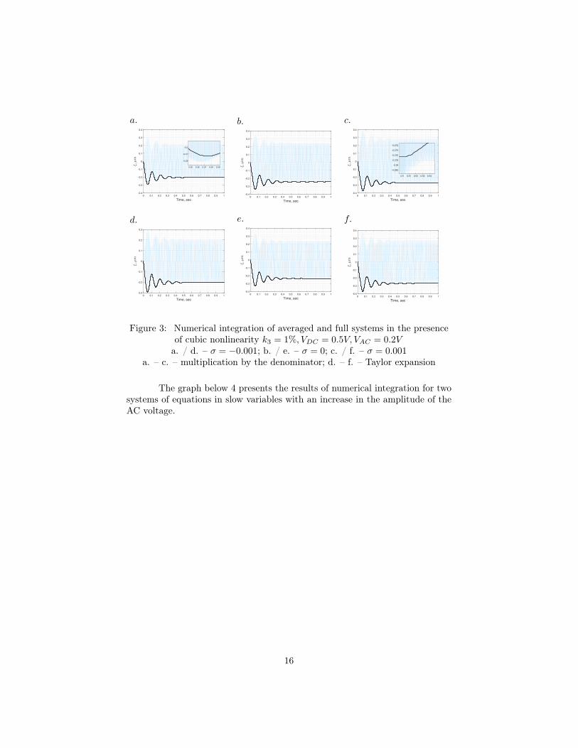
Figure 3: Numerical integration of averaged and full systems in the presenceof cubic nonlinearity k3 = 1%, VDC = 0.5V, VAC = 0.2V

a. / d. – σ = −0.001; b. / e. – σ = 0; c. / f. – σ = 0.001a. – c. – multiplication by the denominator; d. – f. – Taylor expansion

The graph below 4 presents the results of numerical integration for twosystems of equations in slow variables with an increase in the amplitude of theAC voltage.

16

0 0.1 0.2 0.3 0.4 0.5 0.6 0.7 0.8 0.9 1

Time, sec

-1.2

-1

-0.8

-0.6

-0.4

-0.2

0

0.2

Figure 4: Comparison of slowly varying vibration amplitudes for two methodsof deriving the equation

On the graph 4 it can be seen that with an increase in the amplitudeof the impact, the difference between the steady-state oscillation amplitudes forthe two methods increases.

4.2 Static Equilibrium Diagrams and Static Displacement

Function Approximation

Since the purpose of this work is to study the dynamic modes of oper-ation of an electrostatic drive when changing the active parameters of voltagesVDC , VAC and frequency tuning parameter σ, then all other parameters de-pending on the above should be explicitly expressed through them in order tocorrectly describe the influence of active parameters changes on the behavior ofthe system. Among the parameters that depend on active ones, one can name

the dimensionless amplitudes of the electrostatic force λ, λ1 and λ2, dimen-sionless parameter Ω, arising as a result of repeated replacement of the timevariable, as well as the static displacement u0 of the movable electrode underthe action of only the time-independent component of the electrostatic force,which is included in the expression for the Ω parameter and in all the coefficientsCi introduced earlier in Sect. 3. All of the above parameters have an explicitexpression of dependence on active parameters, with the exception of the staticdisplacement u0, which, if the second electrode is not taken into account, canbe found from the equation (4):

u0 + k3u30 =

λ

(1− u0)2.

17

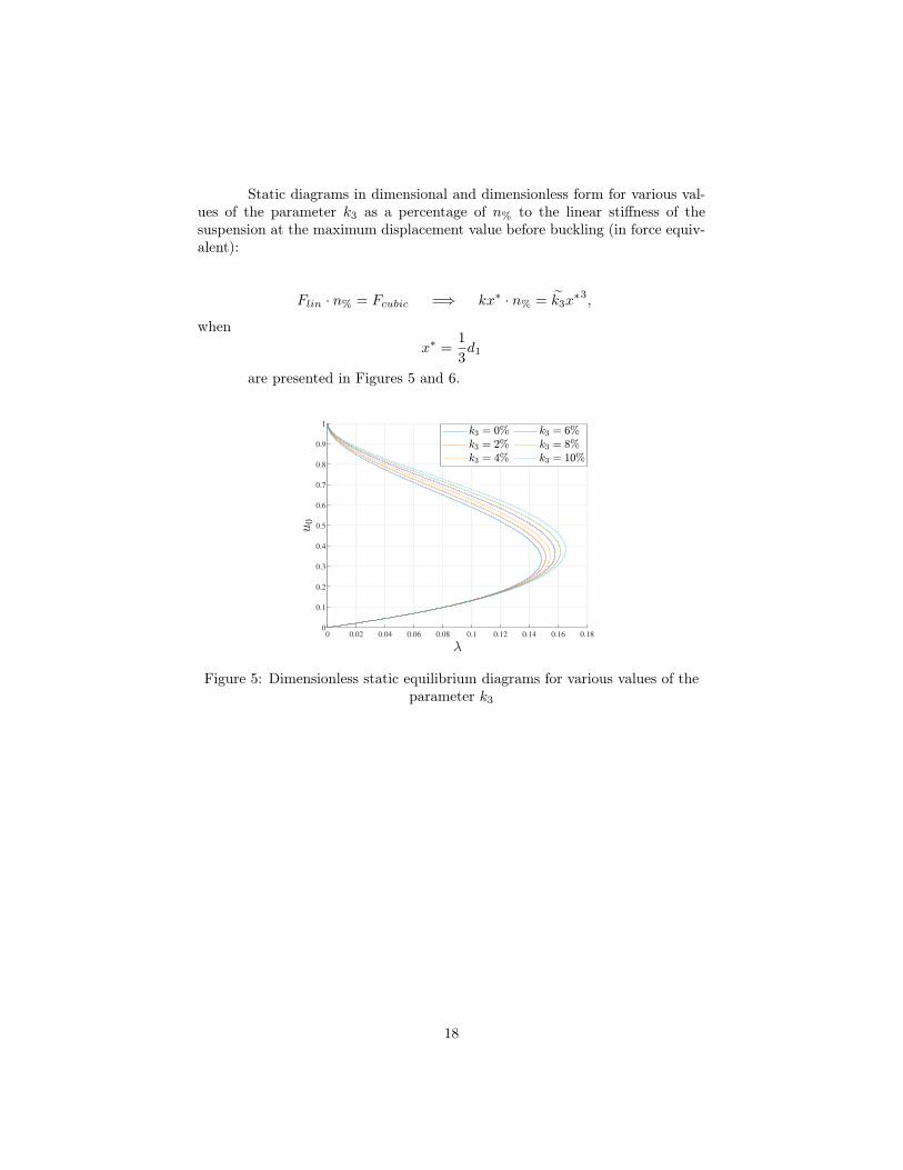
Static diagrams in dimensional and dimensionless form for various val-ues of the parameter k3 as a percentage of n% to the linear stiffness of thesuspension at the maximum displacement value before buckling (in force equiv-alent):

Flin · n% = Fcubic =⇒ kx∗ · n% = k3x∗3,

when

x∗ =1

3d1

are presented in Figures 5 and 6.

0 0.02 0.04 0.06 0.08 0.1 0.12 0.14 0.16 0.180

0.1

0.2

0.3

0.4

0.5

0.6

0.7

0.8

0.9

1

Figure 5: Dimensionless static equilibrium diagrams for various values of theparameter k3

18

0 10 20 30 40 50 60 70

0

0.5

1

1.5

2

2.5

3

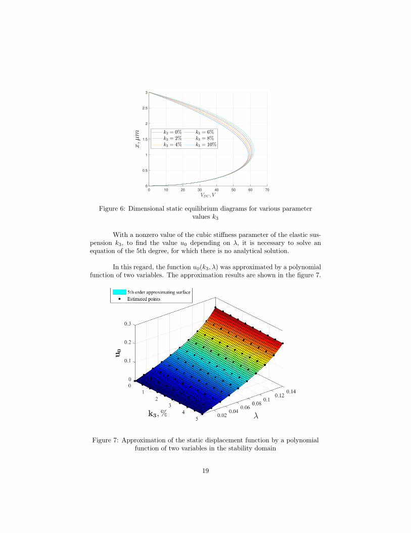
Figure 6: Dimensional static equilibrium diagrams for various parametervalues k3

With a nonzero value of the cubic stiffness parameter of the elastic sus-pension k3, to find the value u0 depending on λ, it is necessary to solve anequation of the 5th degree, for which there is no analytical solution.

In this regard, the function u0(k3, λ) was approximated by a polynomialfunction of two variables. The approximation results are shown in the figure 7.

Figure 7: Approximation of the static displacement function by a polynomialfunction of two variables in the stability domain

19

This graph clearly shows the dependence of the static displacement onthe cubic nonlinearity of the elastic suspension and the constant voltage com-ponent.

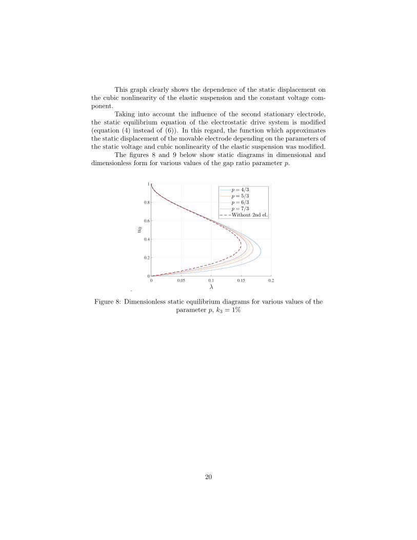
Taking into account the influence of the second stationary electrode,the static equilibrium equation of the electrostatic drive system is modified(equation (4) instead of (6)). In this regard, the function which approximatesthe static displacement of the movable electrode depending on the parameters ofthe static voltage and cubic nonlinearity of the elastic suspension was modified.

The figures 8 and 9 below show static diagrams in dimensional anddimensionless form for various values of the gap ratio parameter p.

0 0.05 0.1 0.15 0.2

0

0.2

0.4

0.6

0.8

1

Figure 8: Dimensionless static equilibrium diagrams for various values of theparameter p, k3 = 1%

20

0 10 20 30 40 50 60 70

0.5

1

1.5

2

2.5

3

Figure 9: Dimensional static equilibrium diagrams for various values of theparameter p, k3 = 1%

4.3 Analysis of the amplitude-frequency response of the

system

As mentioned above, in the obtained systems of equations in slow vari-ables, there are three active parameters – VDC , VAC and σ. In this subsection,the continuation of the solution by the parameter σ will be considered, thatis, as a result, the amplitude and phase-frequency response (APFreqR) of thesystem will be obtained with different variations of the remaining parameters –VDC and VAC for a system of equations in slow variables obtained by expandingthe electrostatic force in a Taylor series.

Hereinafter, continuation by parameter implies continuation of a stableequilibrium position when one of the active parameters changes. Continuationby parameter is implemented using the MATCONT package [Dhooge].

21

a.

2420 2425 2430 2435 2440

0

0.5

2420 2425 2430 2435 2440

-2

0

2

b.

2420 2425 2430 2435 2440

0

0.5

1

2420 2425 2430 2435 2440

-2

0

2

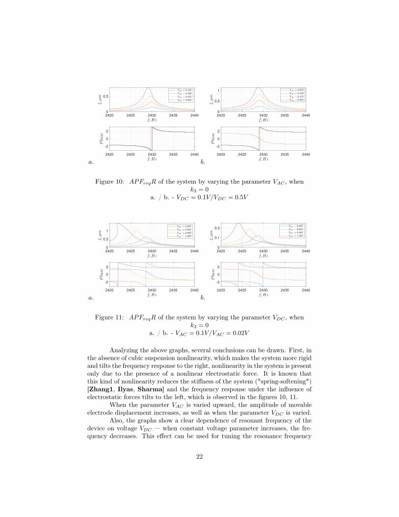
Figure 10: APFreqR of the system by varying the parameter VAC , whenk3 = 0

a. / b. - VDC = 0.1V/VDC = 0.5V

a.

2420 2425 2430 2435 2440

0

0.5

1

2420 2425 2430 2435 2440

-2

0

2

b.

2420 2425 2430 2435 2440

0

0.1

0.2

2420 2425 2430 2435 2440

-2

0

2

Figure 11: APFreqR of the system by varying the parameter VDC , whenk3 = 0

a. / b. - VAC = 0.1V/VAC = 0.02V

Analyzing the above graphs, several conclusions can be drawn. First, inthe absence of cubic suspension nonlinearity, which makes the system more rigidand tilts the frequency response to the right, nonlinearity in the system is presentonly due to the presence of a nonlinear electrostatic force. It is known thatthis kind of nonlinearity reduces the stiffness of the system ("spring-softening")[Zhang1, Ilyas, Sharma] and the frequency response under the influence ofelectrostatic forces tilts to the left, which is observed in the figures 10, 11.

When the parameter VAC is varied upward, the amplitude of movableelectrode displacement increases, as well as when the parameter VDC is varied.

Also, the graphs show a clear dependence of resonant frequency of thedevice on voltage VDC — when constant voltage parameter increases, the fre-quency decreases. This effect can be used for tuning the resonance frequency

22

on required values in some applications.

a.

2410 2420 2430 2440 2450 2460

0

0.2

0.4

2420 2430 2440 2450 2460

-2

0

2

b.

2410 2420 2430 2440 2450 2460

0

0.2

0.4

2420 2430 2440 2450

-2

0

2

4

Figure 12: APFreqR of the system by varying the parameter VAC , whenk3 = 1%

a. / b. - VDC = 0.2V/VDC = 0.05V

a.

2400 2420 2440 2460 2480 2500 2520

0.2

0.4

0.6

0.8

2400 2420 2440 2460 2480 2500 2520

-4

-2

0

2

4

b.

2420 2425 2430 2435 2440

0

0.1

0.2

2420 2425 2430 2435 2440

-2

0

2

Figure 13: APFreqR of the system by varying the parameter VDC , whenk3 = 1%

a. / b. - VAC = 0.1V/VAC = 0.02V

Analyzing the dependences 12 – 13 in comparision with 10 – 11, itcan be concluded, that their clear difference is a slope APFreqR to the rightdue to addition a cubic component of the elastic suspension stiffness, whichincreases the overall rigidy of the system. The graph 14 below shows a seriesof frequency response for different values of the parameter VDC at a fixed valueof the parameter of the cubic nonlinearity of the suspension, demonstrating thechange in the slope of the frequency response with an increase in the influenceof the "soft" nonlinearity of the electric field.

23

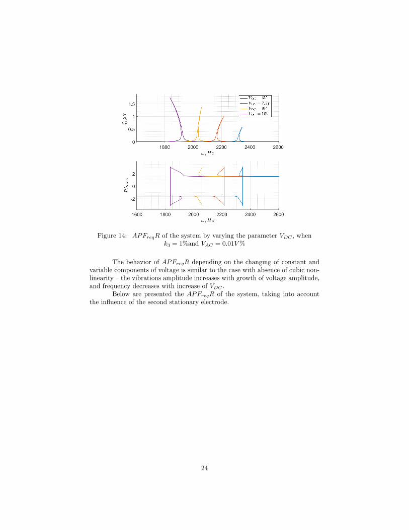
Figure 14: APFreqR of the system by varying the parameter VDC , whenk3 = 1%and VAC = 0.01V%

The behavior of APFreqR depending on the changing of constant andvariable components of voltage is similar to the case with absence of cubic non-linearity – the vibrations amplitude increases with growth of voltage amplitude,and frequency decreases with increase of VDC .

Below are presented the APFreqR of the system, taking into accountthe influence of the second stationary electrode.

24

a.

2420 2425 2430 2435 2440

0

0.5

1

2420 2425 2430 2435 2440

-4

-2

0

2

b.

2400 2450 2500 2550

0

0.5

1

2400 2450 2500 2550

-2

0

2

4

c.

2420 2425 2430 2435 2440

0

0.5

2420 2425 2430 2435 2440

-2

0

2

d.

2400 2420 2440 2460 2480 2500

0

0.2

0.4

0.6

2400 2420 2440 2460 2480 2500

-2

0

2

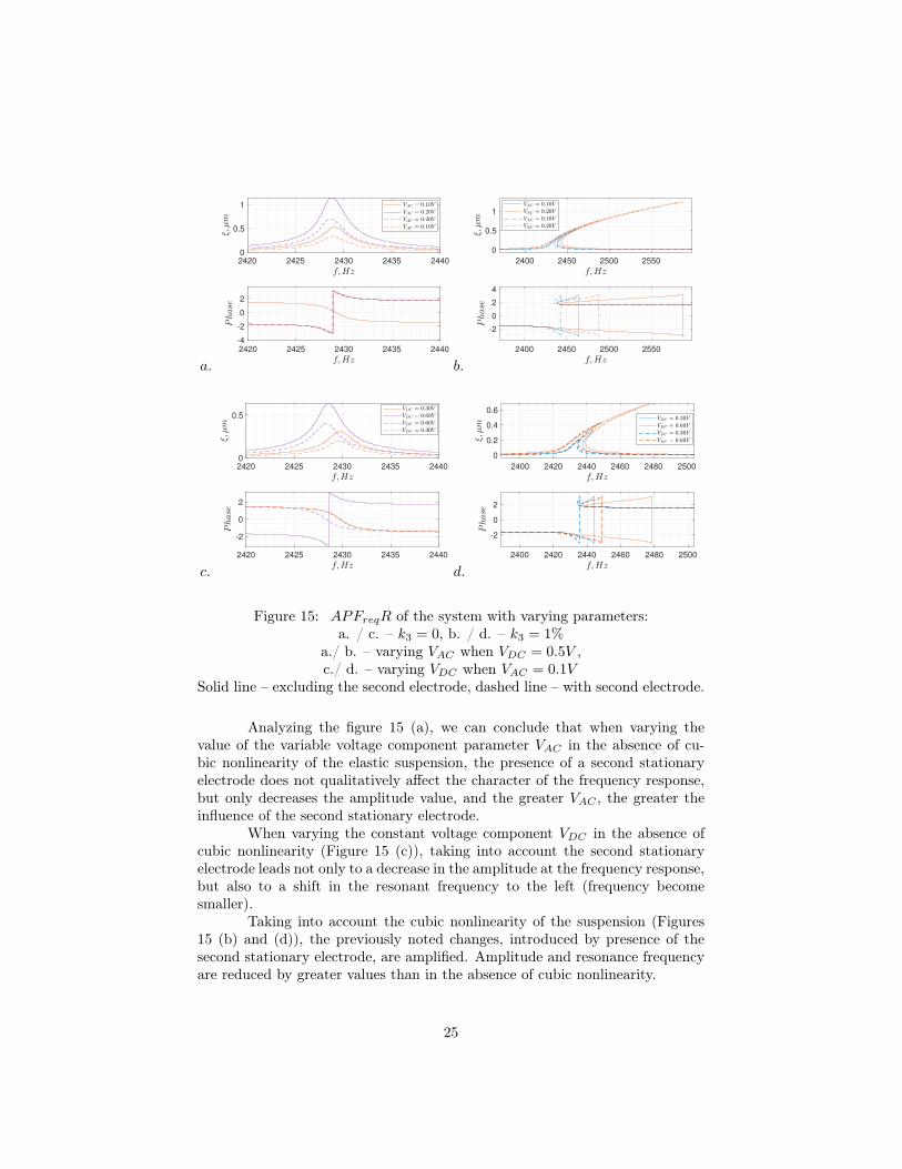
Figure 15: APFreqR of the system with varying parameters:a. / c. – k3 = 0, b. / d. – k3 = 1%

a./ b. – varying VAC when VDC = 0.5V ,c./ d. – varying VDC when VAC = 0.1V

Solid line – excluding the second electrode, dashed line – with second electrode.

Analyzing the figure 15 (a), we can conclude that when varying thevalue of the variable voltage component parameter VAC in the absence of cu-bic nonlinearity of the elastic suspension, the presence of a second stationaryelectrode does not qualitatively affect the character of the frequency response,but only decreases the amplitude value, and the greater VAC , the greater theinfluence of the second stationary electrode.

When varying the constant voltage component VDC in the absence ofcubic nonlinearity (Figure 15 (c)), taking into account the second stationaryelectrode leads not only to a decrease in the amplitude at the frequency response,but also to a shift in the resonant frequency to the left (frequency becomesmaller).

Taking into account the cubic nonlinearity of the suspension (Figures15 (b) and (d)), the previously noted changes, introduced by presence of thesecond stationary electrode, are amplified. Amplitude and resonance frequencyare reduced by greater values than in the absence of cubic nonlinearity.

25

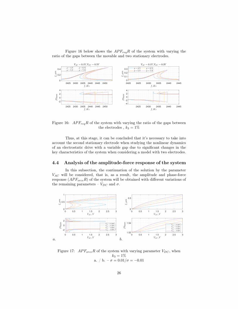
Figure 16 below shows the APFreqR of the system with varying theratio of the gaps between the movable and two stationary electrodes.

2425 2430 2435 2440 2445 2450

0

0.2

0.4

2425 2430 2435 2440 2445 2450

-2

0

2

4

2420 2425 2430 2435 2440 2445

0

0.1

0.2

0.3

2425 2430 2435 2440 2445

-4

-2

0

2

4

Figure 16: APFreqR of the system with varying the ratio of the gaps betweenthe electrodes , k3 = 1%

Thus, at this stage, it can be concluded that it’s necessary to take intoaccount the second stationary electrode when studying the nonlinear dynamicsof an electrostatic drive with a variable gap due to significant changes in thekey characteristics of the system when considering a model with two electrodes.

4.4 Analysis of the amplitude-force response of the system

In this subsection, the continuation of the solution by the parameterVAC will be considered, that is, as a result, the amplitude and phase-forceresponse (APForceR) of the system will be obtained with different variations ofthe remaining parameters – VDC and σ.

a.

0 0.5 1 1.5 2 2.5 3

0

0.5

1

0 0.5 1 1.5 2 2.5 3

-2

0

2

b.

0 0.5 1 1.5 2 2.5 3

0

0.5

0 0.5 1 1.5 2 2.5 3

1.52

1.54

Figure 17: APForceR of the system with varying parameter VDC , whenk3 = 1%

a. / b. – σ = 0.01/σ = −0.01

26

a.

0 0.5 1 1.5 2 2.5 3

0

0.5

0 0.5 1 1.5 2 2.5 3

-2

0

2

b.

0 0.5 1 1.5 2 2.5 3

0

0.5

0 0.5 1 1.5 2 2.5 3

1

1.5

Figure 18: APForceR of the system with varying parameter VDC , whenk3 = 1%

a. / b. – σ = 0.001/σ = −0.001

In the presence of cubic nonlinearity, the frequency response of the sys-tems has a slope to the right, and the APForceR graph shows the change indisplacement when the parameter VAC changes at a certain frequency, that is,when moving along the frequency response from bottom to top along a verticalstraight line passing through the selected frequency value (parameter is fre-quency detuning from resonance). Moreover, the lower branch of the frequencyresponse (on the interval where three displacement values correspond to onefrequency value) is unstable and the modes it describes are not realized. In thisregard, on the APForceR graphs for values of the frequency detuning param-eter greater than 0 (in the region to the right of the resonance), an inflectionin the dependence should be observed with a sharp increase in the amplitudeand subsequent smooth growth with an increase in the parameter VAC , whichis observed in Figures 17 (а) and 18 (a), and the closer to resonance, the lowervoltage values the described effect will be observed.

In the zone before resonance, the dependence of the frequency responseis unambiguous, and therefore the graphs of the APForceR should show just asmooth increase in the amplitude with increasing voltage, which is demonstratedin Figures 17 (b) and 18 (b).

Further, the APForceR of the system will be obtained, taking into ac-count the influence of the second stationary electrode.

27

a.

0 0.5 1 1.5 2 2.5 3

0

0.5

0 0.5 1 1.5 2 2.5 3

-2

0

2

b.

0 0.5 1 1.5 2 2.5 3

0

0.5

0 0.5 1 1.5 2 2.5 3

1.5

1.55

Figure 19: APForceR of the system by varying the ratio of the gaps betweenthe electrodes, k3 = 1%, VDC = 0.2V

a. / b. – σ = 0.005, b. / d. – σ = −0.005Solid line – excluding the second electrode, dashed line – with second electrode.

The analysis of the above graphs leads to the conclusion that outsidethe resonance zone (at σ = −0.005) the influence of the second electrode on theAPForceR of the system is limited by a decrease in the amplitude. However, inthe over-resonance zone (σ = 0.005), the influence of the second electrode onthe slope of the ACH curve is seen.

4.5 Continuation of the resonant-mode solution

The next step is to study the dependence of the resonance point, whichdescribes the desired operating mode of the electrostatic drive, on the valuesof the voltage parameters – VAC and VDC . From a mathematical point ofview, we perform continuation of the bifurcation point of the fold type ("limitpoint") [Kuznetsov] by the frequency detuning parameter when increasing ordecreasing two other active parameters in turn. Figure 20 demonstrates seriesof APFreqR of the system for various values of the parameter VAC .

28

Figure 20: Series of APFreqR for various values VAC

Red dashed line on this graph demonstrates changing of bifurcationpoint by σ with increasing VAC . It must be noted, that when moved alongthis line, not only value of frequency tuning parameter is changing, but alsothe vibrations amplitude. Hence, the graph demonstrating the dependence ofresonant amplitude and frequency on active parameters VAC and VDC , willdefine the values of excitation voltages required to maintain the vibration atgiven resonant frequency with given amplitude, that is a main purpose of thiswork.

4.5.1 Resonant regime dependence on VAC

In this subsection the dependencies of resonant frequency and amplitudeon parameter of the variable voltage component VAC are presented. Calculationsare performed using slow-variable system obtained for Taylor series expansionmethod.

0 0.1 0.2 0.3 0.4 0.5 0.6 0.7 0.8 0.9 1

2400

2420

2440

2460

2480

2500

2520

2540

2560

2580

2600

0.1 0.2 0.3 0.4 0.5 0.6 0.7 0.8 0.9 1

0.5

1

1.5

2

2.5

3

Figure 21: Dependence of the resonant frequency (left) and amplitude (right)on the resonance on parameter VAC

29

Figure 21 on the left shows the dependence of the resonant frequency onVAC . This dependence has a limiting value in the region near zero according tothe parameter VAC , after which it changes its growth pattern. This effect is dueto the fact that not for all values of active parameters, a fold-type bifurcationpoint will be observed on the frequency response, since at low voltage valuesthe frequency response function is unambiguous and does not have an unstablebranch. In this connection, with the continuation of the bifurcation point, nosolutions are observed in this area. This effect is also observed in the figure 21on the right, which shows the dependence of the resonance amplitude on VAC .

Figure 22 below shows the frequency response for different sets of pa-rameter values, chosen so that one of them falls into the zone of existence ofthe solution in the figure 21, and the other into the zone where no solutions areobserved .

Figure 22: APFreqR for different sets of parameter values

The second branch on bifurcation diagram 21, which corresponds toslow growth of the frequency and amplitude with increasing control voltage, isshown by dashed line and demonstrates dependence of the another limit pointof frequency response on voltage. This point is situated in unstable area onfrequency response and not interesting with point of view of dynamic analisysof the comb-drive.

Also figure 21 (right) demonstrates the dependence of the vibrations

30

amplitude on VAC , that was obtained by linear model of electrostatic comb-drive. The linear model does not take into account the cubic component ofthe stiffness of the elastic suspension, and also does not describe the effect offrequency tuning under the influence of an electric field – the frequency doesnot depend on the constant voltage component VDC . The dependence of theamplitude on the variable voltage component was obtained in accordance withthe linear theory of oscillations.

It can be seen that at small values of the parameter VAC , the depen-dences obtained on the linear and nonlinear models coincide, and with an in-crease in the amplitude of the AC voltage, the nonlinear model makes it possibleto more accurately determine the dependence of the moving electrode amplitudeof oscillations on the control voltage value.

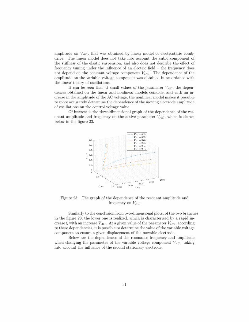
Of interest is the three-dimensional graph of the dependence of the res-onant amplitude and frequency on the active parameter VAC , which is shownbelow in the figure 23.

Figure 23: The graph of the dependence of the resonant amplitude andfrequency on VAC

Similarly to the conclusion from two-dimensional plots, of the two branchesin the figure 23, the lower one is realized, which is characterized by a rapid in-crease ξ with an increase VAC . At a given value of the parameter VDC , accordingto these dependencies, it is possible to determine the value of the variable voltagecomponent to ensure a given displacement of the movable electrode.

Below are the dependences of the resonance frequency and amplitudewhen changing the parameter of the variable voltage component VAC , takinginto account the influence of the second stationary electrode.

31

a.0 0.5 1 1.5 2 2.5 3

2400

2420

2440

2460

2480

2500

2520

2540

2560

2580

2600

b.0 0.5 1 1.5 2 2.5 3

0

0.5

1

1.5

2

2.5

3

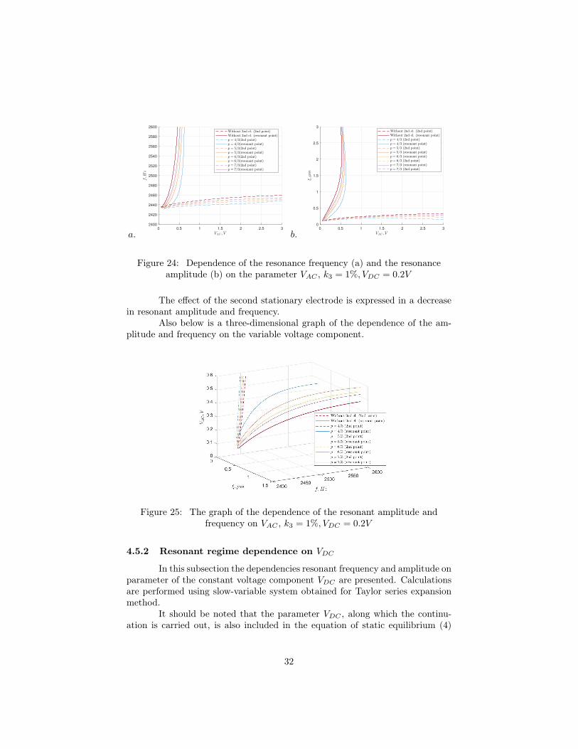
Figure 24: Dependence of the resonance frequency (a) and the resonanceamplitude (b) on the parameter VAC , k3 = 1%, VDC = 0.2V

The effect of the second stationary electrode is expressed in a decreasein resonant amplitude and frequency.

Also below is a three-dimensional graph of the dependence of the am-plitude and frequency on the variable voltage component.

Figure 25: The graph of the dependence of the resonant amplitude andfrequency on VAC , k3 = 1%, VDC = 0.2V

4.5.2 Resonant regime dependence on VDC

In this subsection the dependencies resonant frequency and amplitude onparameter of the constant voltage component VDC are presented. Calculationsare performed using slow-variable system obtained for Taylor series expansionmethod.

It should be noted that the parameter VDC , along which the continu-ation is carried out, is also included in the equation of static equilibrium (4)

32

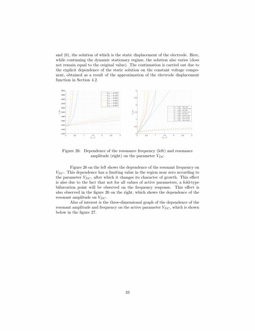
and (6), the solution of which is the static displacement of the electrode. Here,while continuing the dynamic stationary regime, the solution also varies (doesnot remain equal to the original value). The continuation is carried out due tothe explicit dependence of the static solution on the constant voltage compo-nent, obtained as a result of the approximation of the electrode displacementfunction in Section 4.2.

0 0.5 1 1.5 2 2.5 3

2400

2420

2440

2460

2480

2500

2520

2540

2560

2580

2600

0 0.5 1 1.5 2 2.5 3

0

0.5

1

1.5

2

2.5

3

Figure 26: Dependence of the resonance frequency (left) and resonanceamplitude (right) on the parameter VDC

Figure 26 on the left shows the dependence of the resonant frequency onVDC . This dependence has a limiting value in the region near zero according tothe parameter VDC , after which it changes its character of growth. This effectis also due to the fact that not for all values of active parameters, a fold-typebifurcation point will be observed on the frequency response. This effect isalso observed in the figure 26 on the right, which shows the dependence of theresonant amplitude on VDC .

Also of interest is the three-dimensional graph of the dependence of theresonant amplitude and frequency on the active parameter VDC , which is shownbelow in the figure 27.

33

Figure 27: The graph of the dependence of the resonant amplitude andfrequency on VDC

Similarly to the conclusion from two-dimensional plots, of the two branchesin the figure 27, the lower one is realized, which is characterized by a rapid in-crease ξ with an increase VAC . At a given value of the parameter VAC , accordingto these dependencies, it is possible to determine the value of the constant volt-age component to ensure a given displacement of the movable electrode.

In conclusion, similar dependences are presented when taking into ac-count the second stationary electrode when varying the ratio of the gaps betweenthe electrodes.

a.0 0.5 1 1.5 2 2.5 3

2400

2420

2440

2460

2480

2500

2520

2540

2560

2580

2600

b.0 0.5 1 1.5 2 2.5 3

0

0.5

1

1.5

2

2.5

3

Figure 28: Dependence of the resonance frequency (a) and the resonanceamplitude (b) on the parameter VDC , k3 = 1%, VAC = 0.15V

34

Figure 29: Dependence of the resonant amplitude and frequency on VDC ,k3 = 1%, VAC = 0.15V

5 Conclusion

In this paper, an extensive study of the nonlinear dynamics of an elec-trostatic comb-drive with a variable gap is carried out. The amplitude- andphase-frequency response and the amplitude- and phase-force response of thecomb-drive were obtained and analyzed with and without regard to the cubicnonlinearity of the suspension. A decrease in the stiffness of the system underthe action of electrostatic forces ("spring-softening"), as well as a significantvariation of the frequency and force response in the presence of nonlinearity ofan elastic suspension was demonstrated. Using numerical methods of bifurca-tion theory, solutions are obtained that correspond to the resonance peak of thefrequency response when the constant and variable components of the voltageschange. This results makes it possible to determine the range of excitation volt-ages values that provide the required vibrations amplitude in resonant regime.The influence of the second stationary electrode on the dynamics of the sys-tem is estimated. The significant influence of this factor on the resonant-modecharacteristics is revealed.

6 Funding

The research is funded by Russian Science Foundation grant 21-71-10009, https://rscf.ru/en/project/21-71-10009/.

7 Conflict of Interest

The authors declare that they have no conflict of interest.

35

8 References

1. (Iannacci) Iannacci J.: RF-MEMS Technology for High-Performance Pas-sives. IOP Publishing (2017).https://doi.org/10.1088/978-0-7503-1545-6

2. (Varadan) Vijay K. Varadan, K.J. Vinoy, K.A. Jose: RF MEMS and TheirApplications. Wiley (2004).https://doi.org/10.1002/0470856602

3. (Raspopov) Raspopov V.Ya.: Micromechanical devices. Schoolbook. Me-chanical engineering (2007)

4. (Acar) Acar, C., Shkel, A.M.: MEMS Vibratory Gyroscopes: StructuralApproaches to Improve Robustness. Springer (2009)

5. (Shkel) Wang D., Shkel A. M.: Effect of EAM on Quality Factor and Noisein MEMS Vibratory Gyroscopes. 2021 IEEE International Symposium onInertial Sensors and Systems (INERTIAL). — proc., 1-4 (2021).https://doi.org/10.1109/INERTIAL51137.2021.9430471

6. (Pistorio) Pistorio F., Saleem M. M., Soma A. A.: Dual-Mass ResonantMEMS Gyroscope Design with Electrostatic Tuning for Frequency Mis-match Compensation. Applied Sciences. 11(3), 1129 (2021).https://doi.org/10.3390/app11031129

7. (Zhang1) Zhang W. M., Meng G.: Nonlinear dynamic analysis of electro-statically actuated resonant MEMS sensors under parametric excitation.IEEE sensors journal. 7(3), 370-380 (2007).https://doi.org/10.1109/JSEN.2006.890158

8. (Ilyas) Ilyas S. et al.: On the response of MEMS resonators under genericelectrostatic loadings: experiments and applications. Nonlinear Dynam-ics. 95(3), 2263-2274 (2019).https://doi.org/10.1007/s11071-018-4690-3

9. (Rhoads) Rhoads J. F. et al.: Generalized parametric resonance in electro-statically actuated microelectromechanical oscillators. Journal of Soundand Vibration. 296(4-5), 797-829 (2006).https://doi.org/10.1016/j.jsv.2006.03.009

10. (Hajjaj) Hajjaj A. Z. et al.: Linear and nonlinear dynamics of micro andnano-resonators: Review of recent advances. International Journal of Non-Linear Mechanics. 119 (2020).https://doi.org/10.1016/j.ijnonlinmec.2019.103328

11. (Han) Han J. et al.: Mechanical behaviors of electrostatic microresonatorswith initial offset imperfection: Qualitative analysis via time-varying ca-pacitors. Nonlinear Dynamics. 91(1), 269-295 (2018).https://doi.org/10.1007/s11071-017-3868-4

36

12. (Zhang2) Zhang H., Li X., Zhang L.: Bifurcation Analysis of a Micro-Machined Gyroscope with Nonlinear Stiffness and Electrostatic Forces.Micromachines. 12(2), 107 (2021).https://doi.org/10.3390/mi12020107

13. (Zotov) S. A. Zotov, B. R. Simon, A. A. Trusov, A.M. Shkel: High QualityFactor Resonant MEMS Accelerometer With Continuous Thermal Com-pensation. IEEE Sensors Journal. 15(9), 1-1 (2015).https://doi.org/10.1109/JSEN.2015.2432021

14. (Lukin) D. A. Indeitsev, Ya. V. Belyaev, A. V. Lukin, I. A. Popov: Non-linear dynamics of MEMS resonator in PLL-AGC self-oscillation loop.Nonlinear Dynamics. 104(4) (2021).https://doi.org/10.1007/s11071-021-06586-x

15. (Lukin2) D. A. Indeitsev, Ya. V. Belyaev, A. V. Lukin, I. A. Popov,V. S. Igumnova, N. V. Mozhgova: Analysis of imperfections sensitivityand vibration immunity of MEMS vibrating wheel gyroscope. NonlinearDynamics. 105(6), 1-24 (2021).https://doi.org/10.1007/s11071-021-06664-0

16. (Nayfeh) Nayfeh A. H. and Mook D. T.: Nonlinear Oscillations. Wiley(1995)

17. (Kuznetsov) Dhooge, A., Govaerts, W., Kuznetsov, Yu.A.: MATCONT: aMatlab package for numerical bifurcation analysis of ODEs. ACM Trans.Math. Softw. 29, 141-164 (2003). https://doi.org/10.1145/980175.980184

18. (Sharma) Sharma M., Sarraf E. H., Cretu E.: A novel dynamic pull-inMEMS gyroscope. Procedia Engineering. 25, 55-58 (2011).https://doi.org/10.1016/j.proeng.2011.12.014

19. (Kuznetsov2) Kuznetsov Yu. A.: Elements of Applied Bifurcation Theory.Springer (2004)

37