Embed Size (px)
Citation preview

Non-reflecting Boundary Conditions for
Wave Propagation Problems
Daniel Appelo
Stockholm 2003
Licenciate’s ThesisRoyal Institute of Technology
Department of Numerical Analysis and Computer Science

Akademisk avhandling som med tillstand av Kungl Tekniska Hogskolan framlaggestill offentlig granskning for avlaggande av teknisk licentiat-examen fredagen den12 december 2003 kl 10.00 i sal D31, Huvudbyggnaden, Kungl Tekniska Hogskolan,Lindstedtsv 17 , Stockholm.
ISBN 91-7283-628-8TRITA-NA-0326ISSN 0348-2952ISRN KTH/NA/R--03/26--SE
c© Daniel Appelo, December 2003
Hogskoletryckeriet, Stockholm 2003

Abstract
We consider two aspects of non-reflecting boundary conditions for wave propagationproblems. First we evaluate a proposed Perfectly Matched Layer (PML) methodfor the simulation of advective acoustics. It is shown that the proposed PMLbecomes unstable for a certain combination of parameters. A stabilizing procedureis proposed and implemented. By numerical experiments the performance of thePML for a problem with nonuniform flow is investigated. Further the performancefor different types of waves, vorticity and sound waves, are investigated.
The second aspect concerns spurious waves, which are introduced by any dis-cretization procedure. We construct discrete boundary conditions, that are non-reflecting for both physical and spurious waves, when combined with a fourth orderaccurate explicit discretization of one-way wave equations. The boundary conditionis shown to be GKS-stable.
The boundary conditions are extended to hyperbolic systems in two space di-mensions, by combining exact continuous non-reflecting boundary conditions andthe one dimensional discretely non-reflecting boundary condition. The resultingboundary condition is localized by the standard Pade approximation.
Numerical experiments reveal that the resulting method suffers from boundaryinstabilities. Analysis of a related continuous problem suggests that the discreteboundary condition can be stabilized by adding tangential viscosity at the bound-ary. For the lowest order Pade approximation we are able to stabilize the discreteboundary condition.
ISBN 91-7283-628-8 • TRITA-NA-0326 • ISSN 0348-2952 • ISRN KTH/NA/R--03/26--SE
iii

iv

Preface
This thesis consists of an introduction and two papers.
Paper I: Daniel Appelo and Gunilla Kreiss, Evaluation of a Well-posed Per-fectly Matched Layer for Computational Acoustics. In Hyperbolic Problems: The-ory, Numerics, Applications, Proceedings of the Ninth International Conference onHyperbolic Problems (Hyp2002), Pasadena 2002
The author of this thesis contributed to the ideas presented, performed the nu-merical simulations and wrote the manuscript. The author also presented the paperat Hyp2002.
Paper II: Daniel Appelo and Gunilla Kreiss, Stabilized Local Non-reflectingBoundary Conditions for High Order Methods. Technical Report, NADA, RoyalInstitute of Technology, (2003).Presented by the author at ”Waves 2003, Mathematical and Numerical Aspects ofWave Propagation, Jyvaskyla, Finland 30 June - 4 July 2003“Parts of the paper have been published in the proceedings of Waves 2003.
The author contributed to the ideas presented, performed the numerical simu-lations and wrote the manuscript.
1

2
Acknowledgments
I wish to thank my advisor Prof. Gunilla Kreiss, for all her support, guidance andencouragement throughout this work.
I would also like to thank all my friends and colleagues at NADA. Especially Iwould like to thank Katarina Gustavsson and O-P Asen for reading parts of thisthesis and making suggestions for improvement.
Financial support from Vetensakapsradet, Norfa, Generaldirektor WaldemarBorgemans stipendiefond and Erik Petersohns minnesfond is gratefully acknowl-edged.
Finally I want to extend a big and special thanks to Veronica.
3

4
Chapter 1
Introduction
Σ Σ
ΓΩ
ΓΩ
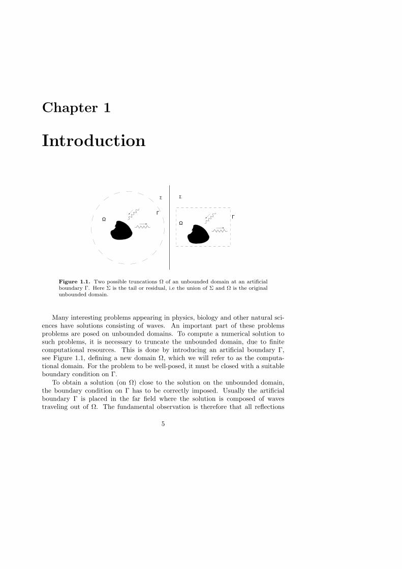
Figure 1.1. Two possible truncations Ω of an unbounded domain at an artificialboundary Γ. Here Σ is the tail or residual, i.e the union of Σ and Ω is the originalunbounded domain.
Many interesting problems appearing in physics, biology and other natural sci-ences have solutions consisting of waves. An important part of these problemsproblems are posed on unbounded domains. To compute a numerical solution tosuch problems, it is necessary to truncate the unbounded domain, due to finitecomputational resources. This is done by introducing an artificial boundary Γ,see Figure 1.1, defining a new domain Ω, which we will refer to as the computa-tional domain. For the problem to be well-posed, it must be closed with a suitableboundary condition on Γ.
To obtain a solution (on Ω) close to the solution on the unbounded domain,the boundary condition on Γ has to be correctly imposed. Usually the artificialboundary Γ is placed in the far field where the solution is composed of wavestraveling out of Ω. The fundamental observation is therefore that all reflections
5

6 Chapter 1. Introduction
caused by the boundary condition on Γ will contaminate the solution in the interior.Hence, an exact boundary condition should prevent all reflections at the boundaryas indicated by the name non-reflecting boundary conditions.
The construction of non-reflecting boundary conditions for wave propagationproblems has been a matter of ongoing research for over thirty years. The levelof difficulty of constructing a particular boundary condition is determined by theunderlying problem. It is possible to divide the boundary conditions into four dif-ferent categories based on the underlying problem. In increasing order of difficultythey are
• Linear time-harmonic wave propagation problems,
• Linear constant coefficient time-dependent wave propagation problems,
• Linear variable coefficient time-dependent wave propagation problems,
• Nonlinear time-dependent wave propagation problems.
To date, there are accurate and efficient boundary conditions available for lineartime-harmonic problems (see the review articles [20, 22, 71]) and we do not considerthis problem here.
For linear constant coefficient time-dependent wave propagation problems, thereare non-reflecting boundary conditions available which work well for some specificproblems. An example is the Maxwell equations, where the perfectly matched layer(discussed below) is used today with satisfactory results. On the other hand, forthe equations of acoustics, the development of efficient non-reflecting boundaryconditions for uniform flows is quite novel.
For the linear variable coefficient time-dependent wave problems and the non-linear time-dependent wave problems very little has been done and there are manychallenging problems left.
In this introduction we consider boundary conditions for linear constant coef-ficient time-dependent wave problems. Particularly we are interested in boundaryconditions which are easy to implementation in a stable and effective fashion, withrespect to both memory and time consumption.
A possible categorization of the non-reflecting boundary conditions available isthe following: exact non-reflecting boundary conditions, local non-reflectingboundary conditions and absorbing boundary layers.
The remaining part of this introduction will be organized as follows. In chapters2-4 we give a brief review of exact non-reflecting boundary conditions, local non-reflecting boundary conditions and absorbing boundary layers. In chapter 5 we givea summary of the presented papers.
Throughout this thesis we will limit the discussion to problems governed bythe wave equation, Maxwell equations and the linearized Euler equations. By lim-ited modifications many of the methods discussed below can be applied to otherequations.

7
Finally we note that there are a number of review articles available which providea more complete overview of the subject [16, 22, 37, 38, 71, 72].

8
Chapter 2
Exact Boundary Conditions
A boundary condition can be defined as a procedure
BEu = 0, on Γ.
Especially, the boundary condition is said to be exact if the solution u, of some PDEclosed with boundary conditions at infinity, on the unbounded domain is identicalto the solution on the bounded domain Ω closed by the boundary condition definedby BE .
Exact boundary conditions, as will be seen below, will in general be nonlocalboth in space and time. The non-locality in time requires the storage of full tem-poral history of the solution on the boundary if the exact boundary condition is tobe used.
In the past, storage requirements have been thought of as an irreparable hin-drance for the use of exact non-reflecting boundary conditions in computations.But, as we will see later, there are novel methods available which reduce storageof the history of the solution. Further, these methods make use of fast algorithmswhich reduce the work per timestep needed to update the exact boundary condi-tions.
The exact boundary condition BE will depend on the shape of Γ and it maybe difficult to find an explicit representation of BE , if the shape of Γ is too com-plicated. In the following sections we will present some exact boundary conditionsfor common choices of Γ.
2.1 Planar Boundaries
We start by considering the construction of exact non-reflecting boundary condi-tions for the two dimensional wave equation in Cartesian coordinates
∂2u
∂t2=∂2u
∂x2+∂2u
∂y2, (2.1)
9

10 Chapter 2. Exact Boundary Conditions
solved on the half plane x ≥ 0.This problem was first considered in the famous paper by Engquist and Majda
[18]. They use that any leftgoing solution u(x, y, t) to (2.1) can be represented by asuperpositions of plane waves traveling to the left. Such plane waves are given by
u = aei(√
ξ2−ω2x+ξt+ωy). (2.2)
Here a is the amplitude and (ξ, ω) are the duals of (t, y) satisfying ξ2−ω2 > 0 andξ > 0.
Engquist and Majda conclude that for fixed (ξ, ω) the condition(d
dx− i
√ξ2 − ω2
)u|x=0 = 0
annihilate plane waves described by (2.2). For that particular plane wave, this willbe an exact non-reflecting boundary condition. For a more general wave packet, theexact non-reflecting boundary condition is obtained by superposition of boundaryconditions for the plane waves, described above. For waves supported by the waveequation, (2.1) the exact non-reflecting boundary condition becomes
F(∂u
∂x
)− i
√ξ2 − ω2Fu = 0, on x = 0,
where Fv(x, ω, ξ) =
∞∫
−∞
∞∫
−∞e−i(ξt+ωy)v(x, y, t) dy dt.
(2.3)
The non-locality of the above boundary condition is clearly manifested throughthe integral transforms. Inverting the transforms directly is not possible since thefunction
√ξ2 − ω2 does not have an explicit inverse transform. To represent (2.3)
in the physical domain, Engquist and Majda use the pseudo-differential operatorwhich has the symbol
√ξ2 − ω2.
Another useful tool which has been used to derive exact boundary conditionsis the Dirichlet to Neumann (DtN) map. The DtN map is an operator relatingthe Dirichlet datum to the Neumann datum on the boundary Γ. This is doneto enforce the desired asymptotic behavior of the solution at infinity. A moreformal definition of the DtN map can be found in e.g. Ramm [60]. Here we restrictourselves to motivating its use by the following example used to derive an alternativeformulation of (2.3).
Consider solutions to the Helmholtz equation posed on the residual domain Σ
s2u = ∇2u, x ∈ Σ, (2.4)
with boundary conditions at infinity identical to those used for Ξ ≡ Σ⋃
Ω. Sinceno boundary condition have been imposed on Γ, there are infinitely many solutionssatisfying the above equation. However, the solution on Ξ must be one of these.

2.1. Planar Boundaries 11
The desired solution u coinciding with the solution on Ξ can be singled out by aspecific choice of the operator D
∂u
∂n= −Du, x ∈ Γ.
D defines the DtN map. Here the normal is taken outward from Ω. The DtN mapcan be used to define the exact boundary condition BE
BEu ≡ ∂u
∂n+ L−1
(DLu
), (2.5)
where L denotes the Laplace transform.Now, (2.5) can be used to derive the exact boundary condition for (2.1) at a
planar boundary. As before we assume that (2.1) is solved for Ω being the half planex > 0. Hence to derive the DtN map we consider solutions which are bounded onΣ. By taking the Fourier and Laplace transform (with the duals (k, s)) of (2.1) weobtain the ordinary differential equation
∂2 ˜u∂x2
= (s2 + |k|2)˜u, x ∈ Σ.
For <s > 0, solutions that are bounded on Σ can be written as
ae√
s2+|k|2x,
and the DtN map is therefore defined by
˜D = −√s2 + |k|2.
Here the the branch of the square root is chosen so that ˜D is analytical and positivefor <s > 0. By inserting ˜D into (2.5) we see that the exact boundary condition isidentical to the boundary condition (2.3) for t > 0.
In [35], Hagstrom derives a formulation of (2.3) which only includes the inverse
Fourier transform in the y direction and a convolution in time. By rewriting ˜D as
˜D = −s− (√s2 + |k|2 − s),
and using that K(s) =√s2 + |k|2 − s for the function
K(t) ≡ J1(t)t
=1π
1∫
−1
√1− ρ2 cos ρt dρ,
Hagstrom obtains the formulation
∂u
∂n− ∂u
∂t−F−1
(|k|2K(|k|t) ∗ Fu) = 0. (2.6)
By the use of fast algorithms for the computation of convolutions, see [41], to-gether with the fast Fourier transform, (2.6) may be directly imposed. The number

12 Chapter 2. Exact Boundary Conditions
of operations required to evaluate the boundary condition would then be acceptable.However the fact that the solution on the boundary has to be stored at all timelevels makes the storage requirements unacceptable for late times. Fortunately, aswe will see later, there is a cure to this.
Note that there is no explicit need for a two dimensional setting in the aboveexamples. The analysis is identical if Γ is chosen as the hyper plane x = 0. TheFourier transform is then to be interpreted as the multidimensional Fourier trans-form.
2.2 Spherical Boundary
Consider the homogeneous wave equation posed on the tail Σ in three dimensions.If the boundary Γ has the shape of a sphere of radius R, we can express the solutionsto Helmholtz equation
s2u = ∇2u, x ∈ Σ,
in spherical harmonics
u =∞∑
l=0
l∑
m=−l
ulm(r)Y ml (θ, φ).
The functions ulm satisfy the equation
∂2ulm
∂r2+
2r
∂ulm
∂r−
(s2 +
l(l + 1)r2
)ulm = 0. (2.7)
As before, we require the solution to be bounded at infinity which leads to thesolution of (2.7)
ulm(r, s) =kl(rs)kl(Rs)
ulm(R, s),
kl(z) =π
2ze−z
l∑
k=0
(l + k)!k!(l − k)!
(2z)−k.
The DtN map is obtained by taking the logarithmic derivative of kl
sk′l(Rs)
kl(Rs)= −s− 1
R− 1RSl, Sl =
∑l−1k=0
(2l−k)!k!(l−k−1)! (2Rs)
k
∑lk=0
(2l−k)!k!(l−k)! (2Rs)
k. (2.8)
By summation over all harmonics, inverse Laplace transform we obtain the exactnon-reflecting boundary condition
∂u
∂r+∂u
∂t
1Ru+
1R2H−1 (Sl ∗ (Hu)l) = 0, r = R, (2.9)
where H denote the spherical harmonic transform. The function Sl is definedthrough its Laplace transform Sl found in (2.8).

2.2. Spherical Boundary 13
A fundamental property of the function Sl is that since its Laplace transformSl is a rational function of degree (l − 1, l) it can be represented as a sum of lexponential functions in the temporal domain. Using the fact that a convolutionbetween an exponential function and a function v(t)
η(t) =∫ t
0
αe−β(t−τ)v(τ) dτ,
can be rewritten as
dη
dt+ βη = αv, v(0) = 0,
it is possible to localize the exact boundary condition (2.9). This was independentlydiscovered by Sofronov [63, 64] and Grote and Keller [30, 31]. In [31] the boundaryconditions (2.9) are used with both finite difference and finite element approxima-tions of the three dimensional wave equation. Numerical simulations are presentedand uniqueness and stability is discussed. Grote and Keller have also successfullyadopted the methods used in [30, 31] to other scattering problems [28, 29, 32, 33].
Since the spherical harmonics decomposition is formulated as an infinite seriesit is necessary to truncate the series at some l ≤ L0. The obvious way to truncateby retaining the first L0 harmonics will lead to extensive memory requirements, ifL0 is large. This is due to the fact that the number of auxiliary variables whichmust be introduced are proportional to L0. Especially this is true if the solutionhas a high harmonic content which means that L0 has to be chosen large.
Norm minimizing rational approximants for convolution kernels are introducedby Alpert et al. in [5, 6]. They make it possible to distribute the error equallyover all harmonics. Alpert et al. study the problem of approximating a convolutionkernel κ(t), as Sl or K, by approximating its Laplace transform κ(s) by a functionK(s) represented as a sum of poles
K(s) =L∑
l=1
pl
s+ sl.
Inverse Laplace transform of K(s). If we require <sl > 0, gives
K(t) =L∑
l=1
ple−slt.
As has been noted above, convolution with the kernel K(t) can be reduced toadvancing L ordinary differential equations with homogeneous initial data.

14 Chapter 2. Exact Boundary Conditions
The motivation of the approximation of the Laplace transformed kernel is foundby using Parseval’s relation on the two convolutions f = K ∗ g and ψ = κ ∗ g
‖f − ψ‖2 = ‖Kg − κg‖2 ≤ ‖K − κ
K ‖∞‖K ∗ g‖2.
Assuming that the kernel κ is approximated with an error in norm ε for m harmon-ics, Alpert et al. are able to prove that this can be done by a fixed small numberof poles L << m. Moreover, for the kernels appearing for a spherical and cylindri-cal boundary, the error bound holds for all times. For example in [5] it is shownthat for 1024 harmonics it is sufficient to use 21 poles for approximating Sl withan error ε ≤ 10−8. This can be compared to the direct truncation which wouldrequire all 1024 harmonics if the solution have high harmonic content close to theboundary. The number of needed auxiliary variables can clearly be reduced by theapproximation technique suggested by Alpert et al.
For the approximation of the kernel used at a planar boundary the error boundhas a weak a dependence on time. But for the 1024 harmonics example discussedabove, ε ≤ 10−8 holds for times t < 10000.
Although (2.9) can be localized in time, it is still nonlocal in space. Therefore,to reduce the operation count it is important to use some fast procedure for thedirect and inverse harmonic transforms. The derivations of such transforms arequite novel and may be found in e.g. Mohlenkamp[57], Suda and Takami [65] andHealy et al. [42].
Ω
ΓΓ1 0
Figure 2.1. The non-reflecting boundary conditions based on retarded potentialssuggested by Ting and Miksis requires two artificial boundaries.
Before considering the construction of exact non-reflecting boundary conditionsfor first order hyperbolic systems, we briefly discuss two additional exact boundaryconditions for the wave equation in three dimensions. The first boundary conditionis based on the exact representation of of the solution by retarded potentials. Itwas originally devised by Ting and Miksis [69] and later implemented by Givoli andCohen [24].

2.2. Spherical Boundary 15
The boundary condition requires two artificial boundaries Γ0 and Γ1 as in Figure2.1. The solution on Γ0 can be represented by the retarded potential formula
u(x, y) = − 14π
∫
Γ1
(u(y, t− r)
∂
∂n
1r− 1r
∂u(y, t− r)∂n
− 1r
∂r
∂n
∂u(y, t− r)∂t
)dy,
(2.10)
r = |x− y|, x ∈ Γ0.
The above formula is nonlocal in time but the temporal history of the solutionneeded to be stored is bounded by the maximum travel time between points onthe boundary. The cost of a direct evaluation of the integral is proportional to thesquare of the points used to discretize the boundary. Again this can be sped-upby fast methods, see [19]. Finally, it should be noted that in the implementationpresented in [24] there was a need for artificial damping to keep the method stable.
lacuna
a a c bcb1 1 1 2 22
0
1
2t
t
t
t
x
front
0
front
reflected
traling
Figure 2.2. Sketch of waves generated by a source with finite support illustratingthe existence of lacuna.
A direct consequence of the formula (2.10) is the strong Huygens’ principle orthe existence of lacunae. The phenomena lacunae can be illustrated by consideringthe wave equation in one dimension with a forcing compactly supported in spaceand time and homogeneous initial data, i.e.
∂2u
∂t2− c2
∂2u
∂x2= f, (2.11)
∂u(x, 0)∂t
= 0, u(x, 0) = 0, (2.12)
supp f = (x, t) |x ∈ [a1, a2], t0 < t < t1. (2.13)
At time t = t0 waves will start to be generated on the domain [a1, a2] as shownin Figure 2.2. At a later time t2, they can at most have traveled to the points b1 and

16 Chapter 2. Exact Boundary Conditions
b2, determined by the wave speed c. Now since waves are only generated betweentimes t0 < t < t1, there will be no waves inside the domain [a1, a2] at times t > t2.The domain [a1, a2] is now inside the lacuna. If we are to construct non-reflectingboundary conditions at a1 and a2 we know that at times t > t2 and t < t0 the exactboundary condition is a homogeneous Dirichlet condition (the existence of lacuna).At the times in between we may compute the solution on a slightly larger domain[c1, c2] with e.g. periodic boundary conditions. The domain [c1, c2] is chosen sothat waves reflected at the boundary does not influence the solution in [a1, a2] fortimes t0 < t < t2.
The existence of lacunae have been used by Ryabenkii, Tsynkov and Turchani-nov [62] to construct exact non-reflecting boundary conditions for the wave equationin odd dimensions by partitioning the source term in time. Note that the existenceof lacunae is restricted to odd space dimensions.
2.3 First Order Hyperbolic Systems
Here we consider construction of exact non-reflecting boundary conditions for a firstorder, constant coefficient, strongly hyperbolic system. The boundary conditionsare imposed at a planar boundary, x = 0. In the domain Ω, (x > 0) the system canbe written as
∂u
∂t+A
∂u
∂x+
∑
j
Bj∂u
∂yj= 0, (2.14)
where u ∈ Rn, A,Bj ∈ Rn×n. If we further assume that A is invertible (no charac-teristic boundary conditions) we can employ the usual Fourier and Laplace trans-form to obtain
∂ ˜u∂x
= M ˜u, M = −A−1
sI +
∑
j
ikjBj
. (2.15)
Since we consider a strongly hyperbolic problem, we can decompose the solution intoleft and right-going modes or waves. The right-going waves are those correspondingto positive eigenvalues of M and the left-going, those who correspond to negativeeigenvalues.
The decomposition
QMQ−1 =[λR 00 λL
]≡ Λ,
where Q is composed of the the eigenvectors of M arranged in two matrices QR, QL
such that
Q =[QR
QL
],

2.3. First Order Hyperbolic Systems 17
can be used to decouple the system into two sets of scalar equations
∂ ˜vL
∂x= λL
˜vL,∂ ˜vR
∂x= λR
˜vR, (2.16)
where ˜v ≡ Q˜u. An exact non-reflecting boundary condition which make sure thatno waves enter Ω at x = 0 is
˜vR ≡ BR˜u = 0. (2.17)
Note that BR can be chosen in many ways. The only restriction of BR is thatit should be orthogonal to the matrix QL. Therefore a natural choice is BR ≡ QR.However this choice may not always be suitable. In fact, it can lead to an ill-posedproblem. This is the case for the linearized Euler equations and was discoveredby Giles in [21], where an alternative choice of BR, which leads to a well-posedproblem, was suggested. Other choices of BR for the linearized Euler equations,leading to a well-posed problem have been suggested by Hagstrom and Goodrich[26, 27] and Colonius and Rowley [61].

18
Chapter 3
Local Non-reflectingBoundary Conditions
In this chapter we begin by presenting some classic local non-reflecting boundaryconditions suggested in the literature. Many of these are formulated as hierarchies ofconditions of increasing accuracy. Often increasing accuracy is synonymous with in-troduction of high-order (mixed) derivatives on the boundary. Stable discretizationof such derivatives is not trivial. Therefore, in practice, the hierarchical structurehave not been exploited properly.
However, boundary conditions containing high-order derivatives can be con-verted into sequences of conditions containing only low order derivatives. Suchboundary conditions are based on the introduction of auxiliary variables and areoften referred to as high-order non-reflecting boundary conditions. Boundary con-ditions of that type will be discussed in the later half of this chapter.
In the previous chapter we discussed the exact boundary condition for the twodimensional wave equation at a planar boundary derived by Engquist and Majda.In [18], Engquist and Majda also present a method to localize the exact boundarycondition. They conclude that if the function
√1− ω2
ξ2
is approximated by some rational function, it is possible to localize the approxima-tion by explicitly inverting the Fourier transforms.
The most natural approximation is perhaps to use a Taylor series expansion,however the resulting local boundary condition leads to an ill-posed problem, andcan therefore not be used.
19
20 Chapter 3. Local Non-reflecting Boundary Conditions
Engquist and Majda investigate the boundary conditions obtained if a Padeexpansion is used. The resulting boundary conditions are proved to yield a well-posed problem independent of the order of the expansion. The boundary conditionsobtained from the two first Pade expansions are
B1u ≡(∂
∂x− 1c
∂
∂t
)u = 0,
B2u ≡(
1c
∂2
∂t∂x− 1c2
∂2
∂t2+
12∂2
∂y2
)u = 0.
Note that in the boundary conditions above, mixed derivatives in time and spaceappear already in the second order approximation, preluding difficulties of dis-cretization of high-order approximations. The above equations are often referredto as one-way equations in the literature.
The Pade expansion is not the only possible approximation, in fact not even thebest (rather the worst at glancing incidence). Other possible expansions (Cheby-shev, least-squares, etc) are studied by Trefethen and Halpern in [40, 70], wherethey also formulate theorems for determining the well-posedness for these types ofexpansions.
Although [18] is the most well known paper that use one-way equations as non-reflecting boundary condition, it should be noted that it was used in an earlier workby Lindeman [54].
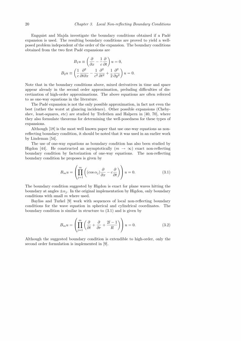
The use of one-way equations as boundary condition has also been studied byHigdon [44]. He constructed an asymptotically (m → ∞) exact non-reflectingboundary condition by factorization of one-way equations. The non-reflectingboundary condition he proposes is given by
Bmu =
m∏
j=1
((cosαj)
∂
∂x− c
∂
∂t
)u = 0. (3.1)
The boundary condition suggested by Higdon is exact for plane waves hitting theboundary at angles ±αj . In the original implementation by Higdon, only boundaryconditions with small m where used.
Bayliss and Turkel [9] work with sequences of local non-reflecting boundaryconditions for the wave equation in spherical and cylindrical coordinates. Theboundary condition is similar in structure to (3.1) and is given by
Bmu =
m∏
j=1
(∂
∂t+
∂
∂r+
2l − 1R
)u = 0. (3.2)
Although the suggested boundary condition is extendible to high-order, only thesecond order formulation is implemented in [9].

3.1. High-Order Local Non-reflecting Boundary Conditions 21
Adoption of the above described classic boundary conditions can be found inmany areas of science where wave propagation is present (see e.g. the review ar-ticles [22, 71]). However, for these boundary conditions, the hierarchical structureis rarely exploited. Typically only the lowest order terms in the expansions areused in the construction. Adoption of the first order Engquist Majda condition toa first order hyperbolic system yields the so called characteristic boundary condi-tions. Independent of application, the solution obtained when a low-order boundarycondition is used will suffer from O(1) error after moderate times.
3.1 High-Order Local Non-reflecting Boundary Con-ditions
Modern high-order local non-reflecting boundary conditions are based on the intro-duction of auxiliary variables. This technique was first used by Collino [13]. Therehe considers the following approximation to the exact boundary condition (2.3)
F(∂u
∂x
)+ iξ
(1−
L∑m=1
βmω2
ξ2 − αmω2
)Fu = 0, x = 0, (3.3)
where the coefficients αm, βm depend on the type of approximation used, L is theorder of the boundary condition. With
αm = cos2(
mπ
2L+ 1
), βm =
22L+ 1
sin2
(mπ
2L+ 1
),
the Pade expansion used in [18] is recovered.Collino shows that the boundary condition (3.3) can be reformulated as a se-
quence of auxiliary problems containing only low order derivatives
∂u
∂x+∂u
∂t−
L∑m=1
βm∂ψm
∂t= 0,
∂2u
∂t2− ∂
∂y2(αmψm + u) = 0, m = 1, . . . , L.
Here ψm are the auxiliary variables introduced on the boundary.In [13] Collino presents numerical experiments using boundary conditions of
different order (L ≤ 10). The results show that the accuracy of the boundarycondition increase monotonically. Long time behavior of the boundary condition isnot examined.
The wave equation posed in a semi infinite wave-guide with a planar boundaryat x = 0 have been considered by Givoli and Neta in [25]. Inspired by the work of
22 Chapter 3. Local Non-reflecting Boundary Conditions
Hagstrom and Harihan (discussed below) they use the Higdon boundary condition(3.1) to formulate a sequence of auxiliary problems
(∂
∂x+
1Cm
∂
∂t
)ψm−1 = ψm, m = 1, . . . , L
ψ0 ≡ u, ψL ≡ 0,(3.4)
which converges to the exact boundary condition (2.3) when L → ∞. Since (3.4)contains normal derivatives of ψm, when discretized, they would need to be storednot only on the boundary but also in the interior. This would be unnecessarymemory consuming and therefore (3.4) is reformulated to contain only tangentialderivatives of second order instead of normal derivatives. In [25] the modifiedboundary conditions are integrated into an explicit finite difference method whichis shown by numerical examples to be stable. Givoli and Neta also give a detaileddescription of how the coefficients Cm can be chosen automatically for good per-formance. It is shown by numerical experiments that accuracy of the method isincreasing with L. This holds for late times.
Hagstrom and Harihan constructed the first reformulation of (3.2) using auxil-iary variables. It was presented in [36, 39] where they consider the wave equationin both spherical and cylindrical coordinates. They also extend the boundary con-dition to the two dimensional Maxwell equations in cylindrical coordinates.
The recursion formula proposed in [39] requires the introduction of L auxiliaryvariables and is given by
(∂
∂t+m
R
)ψm−1 =
12R2
(∇2R +m(m− 2)
)ψm +
12ψm, m = 1, . . . , L,
ψ0 = u, ψL = 0,
where ∇2R is the Laplace operator on a sphere with radius R. The boundary
conditions are implemented using finite differences and results, showing a rapiddecay of the error as L increase, are presented.
In [23], Givoli constructed high-order non-reflecting boundary conditions forthe time-dependent and time-harmonic wave equation in two dimensions in cylin-drical coordinates. Givoli uses that local non-reflecting boundary conditions canbe written on the form
−∂u∂r
= LKu, on Γ,
where LK is a differential operator of order K.By considering the time-harmonic wave equation, Givoli is able to construct
high-order boundary condition which lead to a symmetric finite element discretiza-tion. The method is also extended to the time-dependent case with the symmetricproperties unaltered. Due to symmetry, the resulting finite element discretizationis stable and well-conditioned for all K.

3.1. High-Order Local Non-reflecting Boundary Conditions 23
As we have seen above the operator LK can be formulated with normal or tan-gential derivatives or a mix of both. Givoli derives a boundary condition for anoperator containing only tangential derivatives of even order. To make the bound-ary condition more general, Givoli also give algorithms which translate differentformulations of LK into a form which fit into the high-order boundary condition heproposed. In [23] only results for the time-harmonic wave equation is presented.
We close this section by noting that the high-order non-reflecting boundary con-ditions considered here have been constructed in the context of the wave equation.Due to the the novelty of these methods, extensions to other problems are limitedbut this will surely change with time.

24

Chapter 4
Absorbing Boundary Layers
An alternative to exact or high-order local non-reflecting boundary conditions isto surround the computational domain with a finite width, absorbing layer. Typ-ical setups are pictured in Figure 4.1. Ideally, all waves traveling into the layer,independent of frequency or angle of incidence, should be absorbed to such extentthat reflections at the outermost boundary are of no importance. Absorbing layers
PMLComput.Domain
PMLComput.Domain
Figure 4.1. The computational domain is surrounded by an absorbing layer (PML).Different geometries are possible.
with this ideal properties do exits, and are referred to as Perfectly Matched Layers(PML). They were first introduced in the context of computational electromagnet-ics, where they are considered as state of the art and are widely used in practicalcomputations. Also in computational acoustics the PML technique has had an im-pact. However its performance seems to be not quite as good as for computationalelectromagnetics.
25

26 Chapter 4. Absorbing Boundary Layers
4.1 Absorbing Boundary Layers for ComputationalElectromagnetics
The idea of surrounding the computational domain with an absorbing layer wasstudied by Israeli and Orzag [49] and Kosloff and Kosloff [51]. The proposed ab-sorbing layers only worked well for waves of normal incidence and they where notcommonly used in computations. Karni [50] devise an absorbing layer that is re-flectionless for waves propagating in a given direction but still causes to muchreflections for other waves.
The major breakthrough, which made absorbing boundary conditions com-petitive, was the introduction of the Perfectly Matched Layer by Berenger [12].Berenger considers the form of Maxwell equations describing transverse electrical(T-E) waves in two dimensions
ε0∂Ex
∂t+ σEx =
∂Hz
∂y,
ε0∂Ey
∂t+ σEy = −∂Hz
∂x,
µ0∂Hz
∂t+ σ∗Hz =
∂Ex
∂y− ∂Ey
∂x.
(4.1)
Here Ex and Ey are the electric fields, Hz the magnetic field, ε0 and µ0 are thefree space permittivity and permeability and σ and σ∗ the electric and magneticconductivity. By the simple, but unphysical, splitting Hz = Hzx +Hzy, Berengerintroduced the Perfectly Matched Layer as a medium governed by the equations
ε0∂Ex
∂t+ σxEx =
∂(Hzx +Hzy)∂y
,
ε0∂Ey
∂t+ σyEy = −∂(Hzx +Hzy)
∂x,
µ0∂Hzx
∂t+ σ∗xHzx = −∂Ey
∂x,
µ0∂Hzy
∂t+ σ∗yHzy =
∂Ex
∂y.
(4.2)
For the particular choice σx = σy = σ∗x = σ∗y = 0 (4.2) is reduced to Maxwellequations for vacuum.
In [12], Berenger shows that media described by (σx, σ∗x, 0, 0) or (0, 0, σy, σ
∗y),
where σ and σ∗ satisfy σ∗ε0 = σµ0, does not produce any reflections at a vacuum-medium interface normal to x and y respectively. Furthermore, waves travelingacross the interface decay exponentially inside the media at a rate depending onthe magnitude of the conductivity parameters σ and σ∗.
The equations (4.2) suggest that the conductivity parameters σ and σ∗ shouldbe chosen constant and large for the solution to decay rapidly in the PML. However,

4.1. Absorbing Boundary Layers for Computational Electromagnetics 27
if a constant σ and σ∗ is used in numerical computations there will be reflectionsat the interface due to the discontinuity of σ at the vacuum-medium interface.Instead the conductivity parameters are typically chosen as a function vanishing atthe interface and increasing monotonically to some moderate value at the outermostboundary.
The possibility to tune the conductivity parameters σ and σ∗ is an advantageof the method, but it can also be an inconvenience if it should be chosen auto-matically. To our knowledge there is no known algorithm for an optimal choice ofthe conductivity parameters for a general numerical method although the choice iscritical for the performance of a PML.
Optimal choices of the conductivity parameters have been investigated for spe-cific discretizations by Collino and Monk [15] and Asvadurov et al. [8]. The latterpresents an idea based on optimization of the grid inside the PML rather than theconductivity parameters.
When Berenger introduced his PML the efficiency of it was far better thanpreviously known boundary conditions [66]. Moreover, it was straightforward toimplement and incorporate into existing codes due to its similarity in structure tothe Maxwell equations. These features lead to that the PML-technique was adoptedin many other areas of research. For example Collino constructed PML equationsfor the paraxial equations [14], and for the linearized Euler equations Hu [45] andTam et al. [67] have derived split-field PML equations.
4.1.1 Well-Posed Perfectly Matched Layer
In this section we will discuss the well-posedness (see e.g. [52]) of different PML.Therefore we first introduce the definition of well-posedness for a Cauchy problem.
Definition The Cauchy problem is well-posed if the following two conditions aresatisfied
(I) There exist constants K > 0 and α ∈ R such that for all U(·, 0) ∈ L2 thereexists a unique solution U(·, t) ∈ L2 that satisfies
‖U(·, t)‖L2 ≤ Keαt‖U(·, 0)‖L2 , (4.3)
(II) Any zero order perturbation of the Cauchy problem satisfies (I).
We will also use the concept of a weakly well-posed problem, meaning a problemsatisfying condition (I) but not (II). By this definition a strongly hyperbolic problemis well-posed but a weakly hyperbolic problem can only be weakly well-posed.
Unfortunately the split-field PML introduced by Berenger was shown by Abar-banel and Gottlieb [1] to be only weakly well-posed. It was believed that thesplit-field PML (4.2) could become ill-posed under zero order perturbations. Anexample of such a perturbation for the PML equations was presented in [1].

28 Chapter 4. Absorbing Boundary Layers
Although being only weakly well-posed, the PML of Berenger has been used inpractical computations with success (see e.g. [66]). It also seems that for computa-tions with moderately refined grids, and not too long simulation times, it behaveswell. Recently, Becache and Joly [10] showed by energy estimates that BerngersPML has at worst linearly growing solutions at late times.
There are however several PML formulations for Maxwell equations which arewell-posed. An example is the PML derived by Ziolkowski [74]. Ziolkowski useda Lorenz material model, which is based on physical considerations, to derive anun-split PML. Zhao and Cangelaris use similar ideas in [73], and their PML is oftenreferred to as the standard un-split PML, in the literature. In [59], Petropopoulosderives PML formulations, based on the standard un-split PML, for rectangular,cylindrical and spherical coordinates.
Another PML formulation obtained from mathematical reasoning is proposedby Abarbanel and Gottlieb [2]. They assume that the behavior of the absorbinglayer can be described by lossy Maxwell equations. For a T-E case they start with
∂Ex
∂t=∂Hz
∂y+R1,
∂Ey
∂t= −∂Hz
∂x+R2,
∂Hz
∂t=∂Ex
∂y− ∂Ey
∂x+R3,
(4.4)
and look for solutions satisfying
Hz
Ex
Ey
=
1Ω1(x;α, β, ω)Ω2(x;α, β, ω)
eiω(t−αx−βy)e−α
R x0 σ(η)dη
The unknown functions R1, R2, R3,Ω1,Ω2 are determined by the constraints that
• Ri, (i = 1, 2, 3) should be independent of the parameters α, β, ω,
• the solution should be continuous across the interface,
• the amplitude of the solution vector in the layer should be monotonicallydecreasing.
In the derivation they use the dispersion relation
α2 + β2 = 1, (4.5)
4.1. Absorbing Boundary Layers for Computational Electromagnetics 29
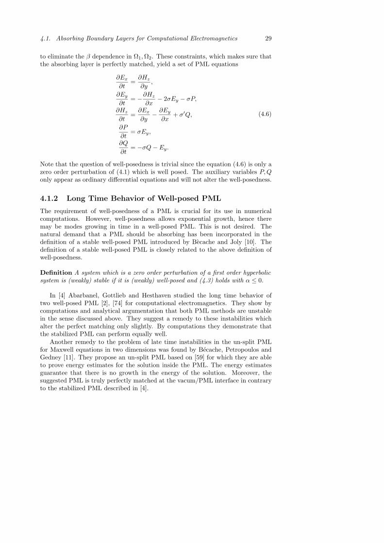
to eliminate the β dependence in Ω1,Ω2. These constraints, which makes sure thatthe absorbing layer is perfectly matched, yield a set of PML equations
∂Ex
∂t=∂Hz
∂y,
∂Ey
∂t= −∂Hz
∂x− 2σEy − σP,
∂Hz
∂t=∂Ex
∂y− ∂Ey
∂x+ σ′Q,
∂P
∂t= σEy,
∂Q
∂t= −σQ− Ey.
(4.6)
Note that the question of well-posedness is trivial since the equation (4.6) is only azero order perturbation of (4.1) which is well posed. The auxiliary variables P,Qonly appear as ordinary differential equations and will not alter the well-posedness.
4.1.2 Long Time Behavior of Well-posed PML
The requirement of well-posedness of a PML is crucial for its use in numericalcomputations. However, well-posedness allows exponential growth, hence theremay be modes growing in time in a well-posed PML. This is not desired. Thenatural demand that a PML should be absorbing has been incorporated in thedefinition of a stable well-posed PML introduced by Becache and Joly [10]. Thedefinition of a stable well-posed PML is closely related to the above definition ofwell-posedness.
Definition A system which is a zero order perturbation of a first order hyperbolicsystem is (weakly) stable if it is (weakly) well-posed and (4.3) holds with α ≤ 0.
In [4] Abarbanel, Gottlieb and Hesthaven studied the long time behavior oftwo well-posed PML [2], [74] for computational electromagnetics. They show bycomputations and analytical argumentation that both PML methods are unstablein the sense discussed above. They suggest a remedy to these instabilities whichalter the perfect matching only slightly. By computations they demonstrate thatthe stabilized PML can perform equally well.
Another remedy to the problem of late time instabilities in the un-split PMLfor Maxwell equations in two dimensions was found by Becache, Petropoulos andGedney [11]. They propose an un-split PML based on [59] for which they are ableto prove energy estimates for the solution inside the PML. The energy estimatesguarantee that there is no growth in the energy of the solution. Moreover, thesuggested PML is truly perfectly matched at the vacum/PML interface in contraryto the stabilized PML described in [4].
30 Chapter 4. Absorbing Boundary Layers
DomainComput.
Mean Flow
PML
x
y
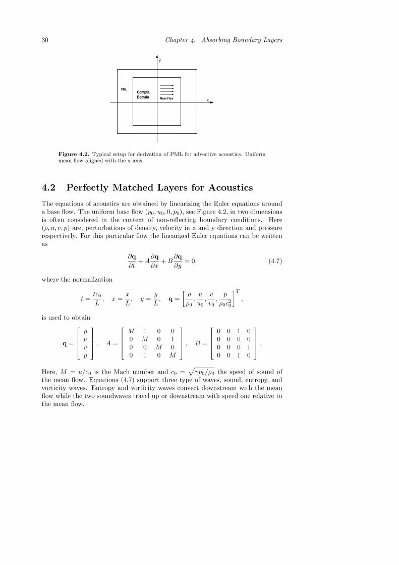
Figure 4.2. Typical setup for derivation of PML for advective acoustics. Uniformmean flow aligned with the x axis.
4.2 Perfectly Matched Layers for Acoustics
The equations of acoustics are obtained by linearizing the Euler equations arounda base flow. The uniform base flow (ρ0, u0, 0, p0), see Figure 4.2, in two dimensionsis often considered in the context of non-reflecting boundary conditions. Here(ρ, u, v, p) are, perturbations of density, velocity in x and y direction and pressurerespectively. For this particular flow the linearized Euler equations can be writtenas
∂q∂t
+A∂q∂x
+B∂q∂y
= 0, (4.7)
where the normalization
t =tc0L, x =
x
L, y =
y
L, q =
[ρ
ρ0,u
u0,v
v0,p
ρ0c20
]T
,
is used to obtain
q =
ρuvp
, A =
M 1 0 00 M 0 10 0 M 00 1 0 M
, B =
0 0 1 00 0 0 00 0 0 10 0 1 0
.
Here, M = u/c0 is the Mach number and c0 =√γp0/ρ0 the speed of sound of
the mean flow. Equations (4.7) support three type of waves, sound, entropy, andvorticity waves. Entropy and vorticity waves convect downstream with the meanflow while the two soundwaves travel up or downstream with speed one relative tothe mean flow.
4.2. Perfectly Matched Layers for Acoustics 31
For ambient acoustics (M = 0), the equations (4.7) become equivalent to theequations describing two dimensional electromagnetics. Hence, stable and well-posed PML formulations are available. For the majority of problems studied inacoustics the flow is advective (M 6= 0) and PML formulations derived for compu-tational electromagnetics do not apply directly. Nevertheless, several ideas how toadopt the PML method to the linearized Euler equations have been suggested.
PML for the linearized Euler equations was first derived by Hu in [45]. Using theapproach of Berenger, Hu adopted the split field formulation to the Euler equationslinearized around an uniform flow pictured in Figure 4.2. Hu later extended hisPML to nonuniform flow and to the fully nonlinear Euler equations [46].
In [45] Hu reported that he had to use a low pass filter inside the absorbinglayer for the solution to remain stable. Hagstrom and Goodrich reported similarobservations in [26]. Later Tam, Auriault and Cambulli [67] proved that the PMLdevised by Hu supported unstable solutions.
Independently Hesthaven [43], following the analysis in [1], proved that the splitPML of Hu was only weakly well-posed. Hesthaven also gave an example of a zeroorder perturbation leading to unbounded growth.
4.2.1 Well-Posed PML for Acoustics
The first well-posed PML for the linearized Euler equations was introduced byAbarbanel, Gottlieb and Hesthaven [3]. They consider isentropic uniform flow forwhich the linearized Euler equations may be written as (4.7) with
q =
ρuv
, A =
M 1 01 M 00 0 M
, B =
0 0 10 0 01 0 0
. (4.8)
If M = 0 the equations (4.7) with (4.8) are identical to the T-E mode equations(4.1) and the PML for that problem can be used.
However if M 6= 0, the dispersion relation becomes much more complicatedand the analysis from electromagnetics is not directly applicable. Abarbanel et al.therefore use a transform of variables
ξ = x, η =√
1−M2y = γy, τ = Mx+ γ2t, (4.9)
and show that the dispersion relation of the transformed equations is the same asof the T-E mode equations discussed in section 4.1.1. In the transformed variablesthey derive a PML which only contains zero order perturbations of the equations(4.7) with (4.8), except for one term
∂Q
∂t= −γ2 ∂ρ
∂y.
By considering the Cauchy problem Abarbanel et al. show that Q is bounded forall times and therefore the PML is well-posed.

32 Chapter 4. Absorbing Boundary Layers
It is interesting to note that the transform of variables (4.9) has been previouslyused by Bayliss and Turkel [9] and later Hu [47]. In [17], Diaz and Joly use thetransformation to construct well-posed PML for the linearized Euler equations.
Recalling the definition used in computational electromagnetics for a stablewell-posed PML it is easy to see that the same requirements should hold for aPML for acoustics. I.e. the PML must be absorbing. To analyze the stability ofthe PML Abarbanel et al. assumed the spatial variations to be small so that theycould remove the spatial derivatives in the PML. The resulting system of ordinarydifferential equations was seen to have solutions growing in time. To remove thisgrowth, they introduced zero order stabilizing profiles which do not alter the well-posedness. But as we shall see below they affect the perfect matching of the PML.
The introduction of the stabilizing profiles was motivated by a separate analysisof a vertical respectively horizontal layer leaving the corners unattended. In [7] weshowed that for a simple choice of damping parameters, the PML is unstable in thecorners.
Another well-posed PML for the linearized Euler equations for a uniform or par-allel flow has been suggested by Hagstrom [38]. The PML suggested by Hagstromis a direct application of a general way to derive perfectly matched layers for hyper-bolic systems in three dimensions described in [38]. In the construction he considersan absorbing layer of width L at the plane x = 0 with the governing equations (forx < 0)
∂u
∂t+A(y)
∂u
∂x+
∑
j
Bj(y)∂u
∂yj+ C(y)u = 0, −L < x < 0. (4.10)
By Laplace transform in time
u = eλxφ,
sI + λA+
∑
j
Bj(y)∂
∂yj+ C(y)
φ = 0, (4.11)
it is possible to find the modal solutions to (4.10).Hagstrom concludes that the solution inside the PML must be modified so that
<λ is bounded away from zero for <s ≥ 0. This guarantees that no generalizedeigenvalues, i.e. <λ → 0 as <s → 0, are present. Moreover if the eigenfunctionsφ are the same at the interface x = 0 the absorbing layer will be truly perfectlymatched.
Postulating a modal solution inside the PML
u = eλx+(λR−1−M−1N)R x0 σ(z)dzφ, (4.12)
and substituting (4.12) into (4.11) gives the resulting PML equations assI + λA(I − σ(R+ σ)−1)
(∂
∂x+ σM−1N
)+
∑
j
Bj(y)∂
∂yj+ C(y)
u = 0.
4.2. Perfectly Matched Layers for Acoustics 33
The choice of the operators M,N and R is not critical by them self. E.g. Hagstromsuggest that the first two can be chosen as numbers. The question is rather how tochoose the combination of them in such a way that all waves are damped. Howeverit is reasonable to choose R to be a first order, constant coefficient, scalar differentialoperator in time and in the transverse variables
R =∂
∂t+
∑
j
βj(y)∂
∂yj+ α.
For the constant coefficient case, the choice of the operators are dictated by analgebraic relation
<(λ+ σ
(λ
R− N
M
))6= 0, <s ≥ 0, σ > 0, (4.13)
which is obtained by taking the Fourier transform in the transverse variables. Here,bar denote the transformed version of the operators.
Applying the above analysis to the equations (4.7) and (4.8) the resulting PMLis governed by the equations
∂q∂t
+A
(∂q∂x
+ µσq)
+B∂q∂y
+ w = 0,
∂w∂t
+ σw + σA
(∂q∂x
+ µσq)
= 0.(4.14)
where w are auxiliary variables, µ = M/(1 −M2) and σ is the damping profile.Contrary to the PML suggested by Abarbanel et al. the PML (4.14) is truly
PMLPML
Ly
+δx xLxLxDomainComput.
y
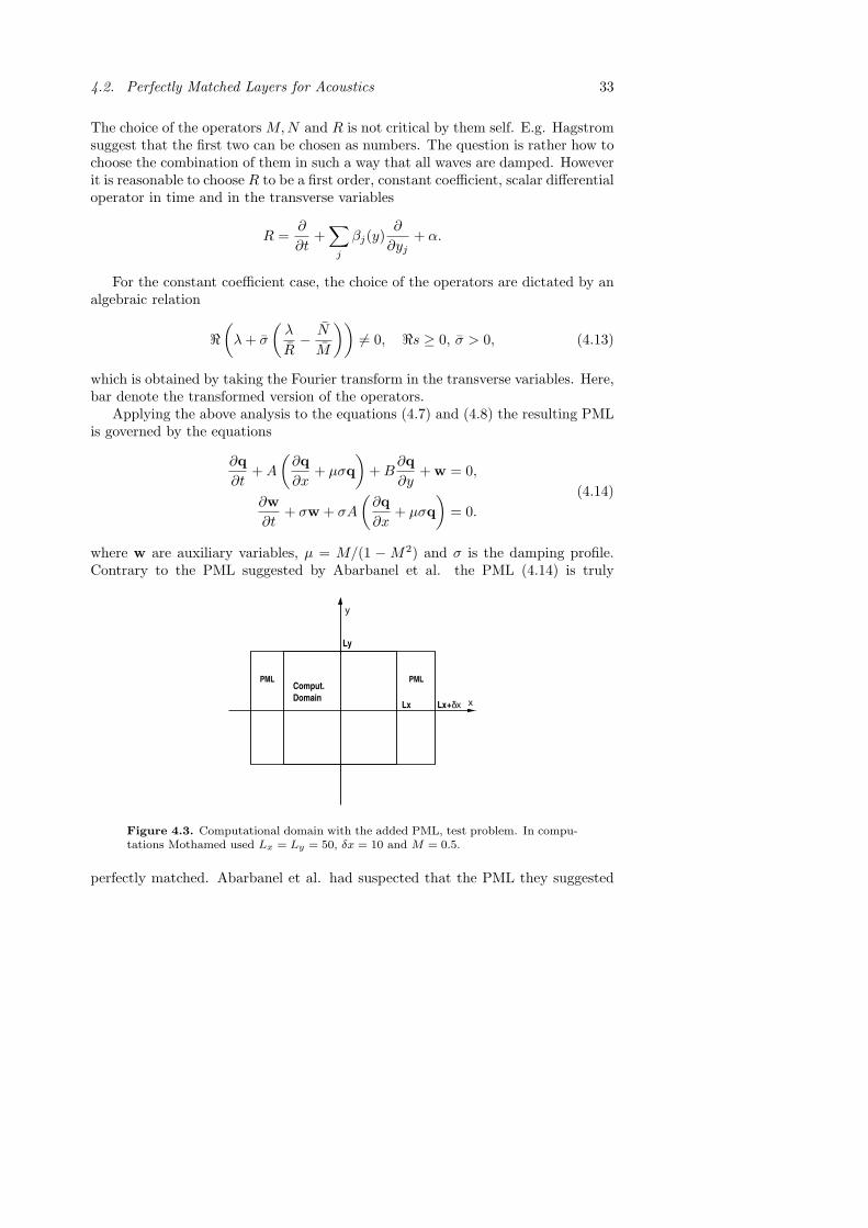
Figure 4.3. Computational domain with the added PML, test problem. In compu-tations Mothamed used Lx = Ly = 50, δx = 10 and M = 0.5.
perfectly matched. Abarbanel et al. had suspected that the PML they suggested
34 Chapter 4. Absorbing Boundary Layers
was not truly perfectly matched after adding stabilizing parameters but did notinvestigate if further. In [58] Motamed showed that this indeed is the case.
Motamed compared the PML suggested by Abarbanel et al. with the PML(4.14) for a test problem adopted from [3]. The domain of the test problem isdescribed in Figure 4.3. Inside the computational domain the components ρ, u, andv where subjected to a continuous forcing. In the y-direction periodic boundaryconditions were used and the PML was terminated by characteristic boundaryconditions.
The equations were discretized by second order centered differences in spaceand advanced in time by the standard fourth order Runge Kutta. The error wasmeasured as the L∞-error along x = 48 using a reference solution computed on alarger domain. Simulations were performed for three successively halved step-sizes.
In Figure 4.4 we see that the L∞-error along the line x = 48 decrease as theresolution is increased for the PML suggested by Hagstrom and also for the PMLsuggested by Abarbanel et al. if no stabilizing profiles are used. If stabilizingprofiles are used in the latter PML the error converges to some fixed value i.e. thePML is not truly perfectly matched.

4.2. Perfectly Matched Layers for Acoustics 35
0 10 20 30 40 50 60 70 80 90 10010
−10
10−9
10−8
10−7
10−6
10−5
10−4
10−3
10−2
10−1
100
PML1, without stabilizing parameteres
time
Inf−
erro
r
dx=dy=1dx=dy=0.5dx=dy=0.25
(a) Error along x=48 for ρ, UnstabilizedPML suggested by Abarbanel et al. If thesimulations are performed for longer timethe solution will not remain stable.
0 10 20 30 40 50 60 70 80 90 10010
−10
10−9
10−8
10−7
10−6
10−5
10−4
10−3
10−2
10−1
100
PML1
time
Inf−
erro
r
dx=dy=1dx=dy=0.5dx=dy=0.25
(b) Error along x=48 for ρ, Stabilized PMLsuggested by Abarbanel et al.
0 10 20 30 40 50 60 70 80 90 10010
−10
10−9
10−8
10−7
10−6
10−5
10−4
10−3
10−2
10−1
100
PML2
time
Inf−
erro
r
dx=dy=1dx=dy=0.5dx=dy=0.25
(c) Error along x=48 for ρ, PML suggestedby Hagstrom
Figure 4.4. All figures are taken from [58].

36

Chapter 5
Summary of Included Papers
5.1 Paper I: Evaluation of a Well-posed PerfectlyMatched Layer for Computational Acoustics
In this paper we present results from numerical experiments where we solve the lin-earized Euler equations and use the PML derived in [3] as non-reflecting boundarycondition.
The first experiment was conducted to understand why PML for acoustics doesnot work as well as PML for Maxwell equation. Therefore, we compare the perfor-mance of the PML for the two different types of waves, vorticity waves and soundwaves, supported by the equations. We also vary the angles of incidence with whichthe waves approach the boundary. To analyze the result we use a wavesplitting tech-nique to decompose the solution into vorticity and sound waves. The computationsshow that the PML is less efficient for vorticity waves than for sound waves.
In a second experiment we investigate how the performance of the PML changeif it is used as boundary condition for a problem with spatially varying mean flow.Remarkably, the change in performance is small although the PML is not designedfor this problem.
We also show, analytically and numerically, that the proposed PML can becomeunstable for a certain combination of parameters. A stabilizing procedure is pro-posed and implemented. Numerical results show that the change in performancefor the stabilized PML is small.
5.2 Paper II: Stabilized Local Non-reflecting Bound-ary Conditions for High Order Methods
In [61] Rowley and Colonius proposed a discretely non-reflecting boundary con-dition for computational acoustics. The boundary condition was designed to be
37

38 Chapter 5. Summary of Included Papers
especially efficient for spurious waves introduced by discretization. The boundarycondition derived in [61] was derived for an implicit scheme of Pade type. Sincedifferent schemes introduce different spurious waves a new discrete boundary con-dition has to be derived for each scheme.
For many problems appearing in acoustics it is more efficient to use an explicitscheme of high-order, rather than an implicit. In paper II we use the frameworkintroduced by Rowley and Colonius to construct a discretely non-reflecting bound-ary condition for the one-way wave equation spatially discretized with the standardexplicit fourth order accurate difference scheme. The boundary condition, whichcan be extended to arbitrary order accuracy, is shown to be GKS-stable for ordersup to at least 8.
Numerical experiments in one dimension show that the discretely non-reflectingboundary condition outperforms characteristic boundary conditions. Especially forcomponents of the solution that are poorly resolved the derived boundary conditionis orders of magnitude better.
The boundary conditions is extended to two space dimensions by combiningexact continuous non-reflecting boundary conditions and the one dimensional dis-cretely non-reflecting boundary condition. The resulting boundary condition islocalized by the standard Pade approximation. By using auxiliary variables thetwo dimensional boundary condition can, in principal , be extended to high-order.However it is found by numerical experiments that the resulting method suffersfrom boundary instabilities.
Analysis of a related continuous problem suggests that the discrete boundarycondition can be stabilized by adding tangential viscosity at the boundary. Forthe lowest order Pade approximation we are able to stabilize the discrete boundarycondition. However, the results of the stabilized boundary condition is not satis-factory. The reflections are smaller than for the characteristic boundary conditionbut does not motivate the extra work needed to implement them.
Bibliography
[1] S. Abarbanel and D. Gottlieb. A mathematical analysis of the pml method.J. Comput. Phys., (134):357, 1997.
[2] S. Abarbanel and D. Gottlieb. On the construction and analysis of absorbinglayers in cem. Appl. Numer. Math., (27):331, 1998.
[3] S. Abarbanel, D. Gottlieb, and J.S Hesthaven. Well-posed perfectly matchedlayers for advective acoustics. J. Comput. Phys., 154:266–283, 1999.
[4] S. Abarbanel, D. Gottlieb, and J.S Hesthaven. Long time behaviour of theperfectly matched layer equations in computational electromagnetics. J. Sci.Comput., 17(1-4):405–422, 2002.
[5] B. Alpert, L. Greengard, and T. Hagstrom. Rapid evaluation of nonreflectingboundary kernels for time-domain wave propagation. SIAM J. Numer. Anal.,37(4):1138–1164, 2000.
[6] B. Alpert, L. Greengard, and T. Hagstrom. Nonreflecting boundary conditionsfor the time dependent wave equation. J. Comput. Phys, 180:270–296, 2002.
[7] D. Appelo and G. Kreiss. Evaluation of a well-posed perfectly matched layerfor computational acoustics. In T.Y. Hou E. Tadmor, editor, Hyperbolic Prob-lems: Theory, Numerics, Applications, Proceedings of the Ninth InternationalConference on Hyperbolic Problems, pages 285–294. Springer Verlag, 2002.
[8] S. Asvadurov, V. Druskin, M.N. Guddati, and L. Knizhnerman. On optimalfinite-difference approximation of pml. SIAM J. Numer. Anal., 41:287–305,2003.
[9] A. Bayliss and E. Turkel. Radiation boundary conditions for wave-like equa-tions. Comm. Pure Appl. Math., 33:707, 1980.
[10] E. Becache and P. Joly. On the analysis of brenger’s perfectly matched layersfor maxwell’s equations. Math. Mod. Numer. Anal., 36(1):87–119, 2002.
39
40 Bibliography
[11] E. Becache, P.G. Petropoulos, and S.D. Gedney. Long-time behavior of theunsplit pml. In E. Heikkola P. Neittaanmki G.C. Cohen, P. Joly, editor, Math-matical and Numerical Aspects of Wave Propagation, Proceedings Waves2003,pages 120–124. Springer Verlag, 2003.
[12] J. Berenger. A perfectly matched layer for the absorption of electromagneticwaves. Journal of Computational Physics, 114:185, 1994.
[13] F. Collino. High order absorbing boundary condiions for wave propagationmodels. straight line boundary and corner cases. In R. Kleinman and et al., ed-itors, Proceedings of the 2nd International Conference on Mathmatical and Nu-merical Aspects of Wave Propagation, pages 161–171. SIAM, Delaware, 1993.
[14] F. Collino. Perfectly matched absorbing layers for the paraxial equations. J.Comput. Phys., 113:164–180, 1997.
[15] F. Collino and P. Monk. Optimizing the perfectly matched layer. SIAM J.Sci. Comp., 19:2061–2090, 1998.
[16] T. Colonius. Modeling artificial boundary conditions for compressible flow.draft version, 2003.
[17] J. Diaz and P. Joly. Stabilized perfectly matched layer for advective acoustics.In E. Heikkola P. Neittaanmki G.C. Cohen, P. Joly, editor, Mathmatical andNumerical Aspects of Wave Propagation, Proceedings Waves2003, pages 115–119. Springer Verlag, 2003.
[18] B. Engquist and A. Majda. Absorbing boundary conditions for the numericalsimulation of waves. Math. Comp., 31:629, 1977.
[19] A. Ergin, B. Shanker, and E. Michielssen. Fast evaluation of three-dimensionaltransient wave fields using diagonal translation operators. J. Comput. Phys,146:157–180, 1998.
[20] K. Gerdes. A review of infinite element methods for exterior helmholtz prob-lems. J. Comput. Acoust., 8(1):43–62, 2000.
[21] M. Giles. Nonreflecting boundary conditions for euler equation calculations.AIAA Journal, 28:2050–2058, 1990.
[22] D. Givoli. Non-reflecting boundary conditions a review. J. Comput. Phys,94:1–29, 1991.
[23] D. Givoli. High-order nonreflecting boundary conditions without high-orderderivatives. J. Comput. Phys, 170:849–870, 2001.
[24] D. Givoli and D. Cohen. Non-reflecting boundary conditions based on kischoff-type formulae. J. Comput. Phys., 117:102–113, 1995.
Bibliography 41
[25] D. Givoli and B. Neta. High-order non-reflecting boundary scheme for time-dependent waves. J. Comput. Phys, 186:24–46, 2003.
[26] J.W. Goodrich and T. Hagstrom. A comparison of two accurate boundarytreatments for computational aeroacoustics. Technical Report 97-1585, AIAA,1999.
[27] J.W. Goodrich and T. Hagstrom. Accurate radiation coundary conditions forthe linearized euler equations in cartesian domains. to appear, 2003.
[28] M. Grote. Non-reflecting boundary conditions for electromagnetic scattering.Int. J. Numer. Model., (13):397–416, 2000.
[29] M. Grote. Nonreflecting boundary conditions for elastodynamic scattering. J.Comput. Phys., (161):331–353, 2000.
[30] M. Grote and J. Keller. Exact nonreflecting boundary conditions for the timedependent wave equation. SIAM J. Appl. Math., (55):280–297, 1995.
[31] M. Grote and J. Keller. Nonreflecting boundary conditions for time dependentscattering. J. Comput. Phys., 127:52–81, 1996.
[32] M. Grote and J. Keller. Nonreflecting boundary conditions for maxwell’s equa-tions. J. Comput. Phys., (139):327–324, 1998.
[33] M. Grote and J. Keller. Nonreflecting boundary conditions for elastic waves.SIAM J. Appl. Math., (60):803, 2000.
[34] M.N. Guddati and J.L Tassoulas. Continued-fraction absorbing boundary con-ditions for the wave equation. J. Comp. Acoust., 8(1):139–156, 2000.
[35] T. Hagstrom. On high-order radiation boundary conditions in. In B. Engquistand G. Kriegsmann, editors, IMA Volume on Computational Wave Propaga-tion, pages 1–22. Springer, New York, 1996.
[36] T. Hagstrom. Progressive wave expansions and open boundary problems. InB. Engquist and G. Kriegsmann, editors, IMA Volume on Computational WavePropagation, pages 23–43. Springer, New York, 1996.
[37] T. Hagstrom. Radiation boundary conditions for the numerical simulation ofwaves. Acta. Numer., 8:47–106, 1999.
[38] T. Hagstrom. New results on absorbing layers and radiation boundary condi-tions. preprint, 2003.
[39] T. Hagstrom and S.I. Hariharan. A formulation of asymptotic and exactboundary conditions using local operators. Appl- Numer. Math., 27:403–416,1998.
42 Bibliography
[40] L. Halpern and L.N. Trefethen. Wide-angle one-way wave equations. J. Acoust.Soc. Am., 84:1397–1404, 1988.
[41] E. Harrier, C. Lubich, and M. Schlichte. Fast numerical solution of nonlinearvolterra convolutional equations. SIAM J. Sci. Stat. Comput., 6:532–541, 1985.
[42] D. Healy, D. Rockmore, P. Kostelec, and S. Moore. Ffts for the 2-sphere,improvments and variations. Adv. Appl. Math., 2002 to appear.
[43] J.S. Hesthaven. On the analysis and construction of perfectly matched layersfor the linearized euler equations. J. comput. Phys., 142:129–147, 1998.
[44] R.L. Higdon. Absorbing boundary conditions for difference approximations tothe multidimensional wave equation. Math. Comp., 47:437–459, 1986.
[45] F. Q. Hu. On absorbing boundary conditions for linearized euler equations bya perfectly matched layer. J. Comput. Phys., 129:201–209, 1996.
[46] F. Q. Hu. On perfectly matched layer as a boundary condition. TechnicalReport 96-1664, AIAA, 1996.
[47] F. Q. Hu. A stable perfectly matched layer for linearized euler equations inunsplit physical variables. J. Comput. Phys., 173:455–480, 2001.
[48] R. Huan and L.L. Thompson. Accurate radiation boundary conditions for thetime-dependent wave equation on unbounded domains. Int. J. Numer. Meth.Engrg., 47:1569–1603, 2000.
[49] M. Israeli and S.A. Orzag. Approximation of radiation boundary conditions.J. Comput. Phys., 41:115–135, 1981.
[50] S. Karni. Far-field filtering operators for supression of reflections of artificialboundaries. SIAM J. Numer. Anal., 33:1014–1047, 1996.
[51] R. Kosloff and D. Kosloff. Absorbing boundaries for wave propagation prob-lems. J. Comput. Phys., 63:363–376, 1986.
[52] H-O. Kreiss and J. Lorenz. Initial-Boundary Value Problems and the Navier-Stokes Equations. Academic Press Inc., 1989.
[53] M. Lassas, J. Liukkonen, and E. Somersalo. Complex riemannian metric andabsorbing boundary conditions. J. Math. Pures Appl., 80(7):739–768, 2001.
[54] E. L. Lindman. ”free space” boundary conditions for the time dependent waveequation. J. Comput. Phys., 18:66–78, 1975.
[55] J.L. Lions, J. Metral, and O. Vacus. Well-posed absorbing layer for hyperbolicproblems. Numer. Math., 92:535–562, 2002.
Bibliography 43
[56] C. Lubich and M. Schlichte. Fast convolution for nonreflecting boundary con-ditions. SIAM J. Sci. Comput., 24(1):161–182, 2002.
[57] M. Mohlenkamp. A fast transform for spherical harmonics. J. of Fourier Anal.and Applic., 5:159–184, 1999.
[58] M. Motamed. Pml methods for aero acoustics computations. Master’s thesis,KTH, 2003.
[59] P.G. Petropolus. Reflectionless sponge layers as absorbing aboundary condi-tions for the numerical solution of maxwell equations in rectangular, cylindricaland spherical coordinates. SIAM J. Appl. Math., 60(3):1037–1058, 2000.
[60] A. Ramm. Scatering by obstacles. D. Reidel, Dordrecht, Netherlands, 1986.
[61] C. W. Rowley and T. Colonius. Discretely nonreflectiing boundary conditionsfor linear hyperbolic systems. J. Comput. Phys., 157:500–538, 2000.
[62] V.S. Ryaben’kii, S.V. Tsynkov, and V.I. Turchaninov. Global discrete artificialboundary conditions for time dependant wave propagation. J. Comput. Phys.,174:712–758, 2001.
[63] I. Sofronov. Conditions for complete transparency on the sphere for the threedimensional wave equation. Russian Acad. Sci. Dokl. Math., (46):397–401,1993.
[64] I. Sofronov. Artificial boundary conditions of absolute transparency for two-and three-dimensional external time-dependent scatering problems. Euro. J.Appl. Math., (9):561–588, 1998.
[65] R. Suda and M. Takami. A fast spherical harmonics transform algorithm.Math. Comp, (71):703–715, 2002.
[66] A. Taflove. Computational Electromagnetics The Finite-Difference Time-Domain Method. Artech House, 1995.
[67] C. K. W. Tam, L. Auriault, and F. Cambuli. Perfectly matched layer as anabsorbing boundary condition for the linearized euler equations in open andducted domains. J. Copmyt. Phys., 144:213–234, 1998.
[68] L.L. Thompson and R. Huan. Implementation of exact non-reflecting boundaryconditions in the finite element method for the time-dependent wave equation.Comput. Meth. Appl. Mech. Engrg., 187:137–159, 2000.
[69] L. Ting and M.J. Miksis. Exact boundary conditions for scattering problems.J. Acoust. Soc. Amer., 80:1825–1827, 1986.
[70] L.N. Trefethen and L. Halpern. Well-posedness of one-way wave equations andabsorbing boundary conditions. Math. Comp., 176:421–435, 1986.

44 Bibliography
[71] S.V. Tsynkov. Numerical solution of problems on unbounded domains, a re-view. Appl. Numer. Math., 27:465–532, 1998.
[72] E. Turkel and A. Yefet. Absorbing pml boundary layers for wave-like equations.Appl. Numer. Math., 27:533–557, 1998.
[73] L. Zhao and A.C. Cangellaris. Gt-pml: Generalized therory of perfectlymatched layers and its application to reflectionless truncation of finite-difference time-domain grids. IEEE Trans. Microwave Theory Tech., 44:2555–2563, 1996.
[74] R. Ziolkowski. Time-derivative lorenz-material model based absorbing bound-ary condition. IEEE Trans. Antennas Propagation, 45:1530–1535, 1997.

Evaluation of a well-posed Perfectly MatchedLayer for Computational Acoustics
Daniel Appelo1 and Gunilla Kreiss1
1 NADA, KTH, Sweden [email protected] NADA, KTH, Sweden [email protected]
1 Introduction
Accurate numerical simulations of wave phenomena are important in manyfields, for example in electro magnetics, seismics and acoustics. We are inter-ested in aeroacoustic problems with a non-vanishing mean flow. The govern-ing equations are the Euler equations. In a typical aeroacoustic situation thesolution consists of a slowly varying mean flow with an added small amplitudeacoustic wave.
The simulations must in general be confined to truncated domains, muchsmaller than the physical space where the phenomena takes place. At theartificial boundary, where the truncation takes place, boundary conditionsmust be set. Ideally the solution of the problem in the truncated domain isidentical to the solution of the original problem. However, often undesirableeffects, such as reflections, limit the accuracy of the solution of the trun-cated problem. Boundary conditions that do not cause reflections are calledabsorbing or non-reflecting boundary conditions
Some of the earliest absorbing or non-reflecting boundary conditionswere derived for the wave equation by Engquist and Majda [6] and Baylissand Turkel [4]. For an overview of the subsequent development of absorb-ing boundary conditions for wave propagation problems, see for instanceHagstrom [8].
For Mawell’s equations an important advance is the derivation of perfectlymatched layers (PML) by Berenger [5] in 1994. The idea of the PML is tosurround the computational domain with an highly absorbing layer in whichthe outgoing waves is attenuated. The governing equations of the absorbinglayer must be matched with the equations of the computational domain, i.e.there should be no reflection at the interface of incoming waves, independentof their angle of incidence and frequency. Berenger introduced a splitting ofthe equations to obtain the additional degrees of freedom needed to matchthe equations at the interface. The resulting PML was orders of magnitudebetter than earlier Absorbing Boundary conditions (ABC’s). One serious dis-advantage of Berengers PML, discovered by Abarbanel and Gottlieb [1], wasthat the splitted set of PDE’s was only weakly well-posed. Other derivationsof a PML for Maxwel’s equations which are well-posed have been presented[2], and are as efficient as Berengers PML. Today PML is commonly used incommercial CEM software.

2 Daniel Appelo and Gunilla Kreiss
In 1996 Hu [10] derived a PML for the Euler equations, linearized atconstant flow, by using the splitting technique introduced by Berenger. Ananalysis of this PML showed that it is only weakly well-posed[9]. In 1998Abarbanel, Gottlieb and Hesthaven [3] derived a well-posed PML. However,the PML technique has so far not been as succesfull for the linearized Eulerequations as for the Maxwells equations. This is true even in the case ofvanishing mean flow. One difference, which may be important is the presenceof vorticity waves.
In this paper we present results from numerical experiments where wesolve the linearized Euler equations and use the PML derived in [3] as ABC.
In one experiment we compare the performance of the PML for the twodifferent types of waves, vorticity waves and sound waves, that are supportedby the equations. We have also varied the angles of incidence with which thewaves approach the boundary. To analyze the result we use the wavesplittingtechnique of Wilson [7], described in Jensen, Efraimsson [11], to decomposethe solution into the different waves. The computations show that the PMLis less efficient for vorticity waves than for sound waves.
In an other experiment we vary the mach number spatially. Computationsshow that varying Mach number does not effect the performance of the PMLsignificantly.
2 The PML and test problems
The PML in [3] is derived for the Euler equations linearized around an isen-tropic uniform (aligned to the x-axis) flow on a rectangular domain repre-sented in Cartesian coordinates. The equations are nondimensionalized withthe Mach number M . In all cases with constant M we have used M = 0.5.The PML is derived in a transformed coordinate system. The transformation(x, y, t) → (ξ, η, τ) is defined by
ξ = x, η =√
1−M2y = γy, τ = Mx + γ2t. (1)
Eigenvalues belonging to plane wave solutions of the transformed problemsatisfy a simple dispersion relation which simplifies the derivation of the PML.The derivation is done separately for the ξ- and η-direction, resulting intwo sets of well-posed perfectly matched layers, which are added together,overlapping each other in the corners. The PML is transformed back to thephysical coordinate system (x, y, t) yielding,
Evaluation of a well-posed PML 3
∂v
∂t+ M
∂v
∂x+
∂ρ
∂y=− σxv + 2σxQx + σ2
xRx + Mσ′xPx
+ 2σyQy + σ2yRy + σy
′Py − εxv + 2µyQy,
∂u
∂t+ M
∂u
∂x+
∂ρ
∂x=− σxu− σxMρ− µyu,
∂ρ
∂t+ M
∂ρ
∂x+
∂u
∂x+
∂v
∂y=− σxρ− σxMu− µyρ,
∂Qx
∂t=− γ2 ∂ρ
∂y, (2)
∂Qy
∂t=γ2č∂ρ
∂y− 2σyQy − σ2
yRy − σy
′Py + σxv
− 2σxQx − σ2xRx −Mσ
′xPx + µxv − 2µyQy
ď,
∂Px
∂t=γ2 [v − σxPx − εxPx] ,
∂Py
∂t=γ2 [ρ− σyPy] ,
∂Rx
∂t=γ2 [Qx − µxRx] ,
∂Ry
∂t=γ2 [Qy − µyRy] .
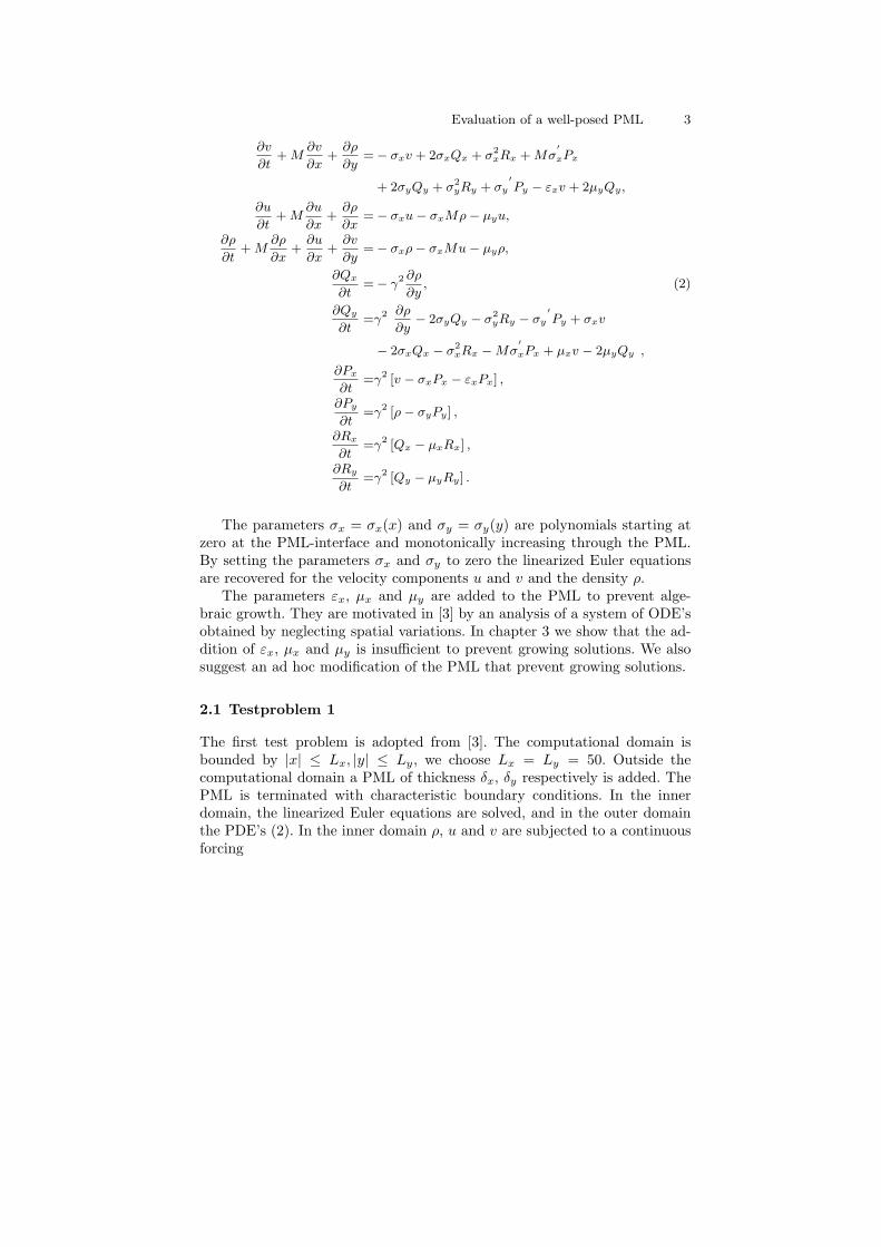
The parameters σx = σx(x) and σy = σy(y) are polynomials starting atzero at the PML-interface and monotonically increasing through the PML.By setting the parameters σx and σy to zero the linearized Euler equationsare recovered for the velocity components u and v and the density ρ.
The parameters εx, µx and µy are added to the PML to prevent alge-braic growth. They are motivated in [3] by an analysis of a system of ODE’sobtained by neglecting spatial variations. In chapter 3 we show that the ad-dition of εx, µx and µy is insufficient to prevent growing solutions. We alsosuggest an ad hoc modification of the PML that prevent growing solutions.
2.1 Testproblem 1
The first test problem is adopted from [3]. The computational domain isbounded by |x| ≤ Lx, |y| ≤ Ly, we choose Lx = Ly = 50. Outside thecomputational domain a PML of thickness δx, δy respectively is added. ThePML is terminated with characteristic boundary conditions. In the innerdomain, the linearized Euler equations are solved, and in the outer domainthe PDE’s (2). In the inner domain ρ, u and v are subjected to a continuousforcing
4 Daniel Appelo and Gunilla Kreiss
ρf (x, y, t) = e−(ln2)
(x−xa)2+(y−ya)2
δ2a sin
(πt
10
),
uf (x, y, t) = 0.05(y − yb)e−(ln2)
(x−xb)2+(y−yb)2
δ2b sin
(πt
10
), (3)
vf (x, y, t) = −0.05(x− xb)e−(ln2)
(x−xb)2+(y−yb)2
δ2b sin
(πt
10
),
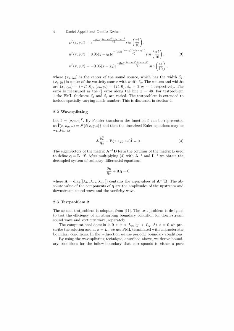
where (xa, ya) is the center of the sound source, which has the width δa,(xb, yb) is center of the vorticity source with width δb. The centers and widthsare (xa, ya) = (−25, 0), (xb, yb) = (25, 0), δa = 3, δb = 4 respectively. Theerror is meassured as the l22 error along the line x = 48. For testproblem1 the PML thickness δx and δy are varied. The testproblem is extended toinclude spatially varying mach number. This is discussed in section 4.
2.2 Wavesplitting
Let f = [ρ, u, v]T . By Fourier transform the function f can be representedas f(x, ky, ω) = Ff(x, y, t) and then the linearized Euler equations may bewritten as
A∂ f∂x
+ B(x, iky, iω)f = 0. (4)
The eigenvectors of the matrix A−1B form the columns of the matrix L usedto define q = L−1f . After multiplying (4) with A−1 and L−1 we obtain thedecoupled system of ordinary differential equations
∂q∂x
+ Λq = 0,
where Λ = diag([λds, λus, λvor]) contains the eigenvalues of A−1B. The ab-solute value of the components of q are the amplitudes of the upstream anddownstream sound wave and the vorticity wave.
2.3 Testproblem 2
The second testproblem is adopted from [11]. The test problem is designedto test the efficiency of an absorbing boundary condition for down-streamsound wave and vorticity wave, separately.
The computational domain is 0 < x < Lx, |y| < Ly. At x = 0 we pre-scribe the solution and at x = Lx we use PML terminated with characteristicboundary conditions. In the y-direction we use periodic boundary conditions.
By using the wavesplitting technique, described above, we derive bound-ary conditions for the inflow-boundary that corresponds to either a pure

Evaluation of a well-posed PML 5
downstream plane sound wave solution or a pure vorticity plane-wave solu-tion with amplitude 1.
Fixing the height of the computational domain to |y| ≤ Ly = 50 andthe wave number ky = 2π/100 the solution is periodic in the y-direction.By specifying different frequencies ω we obtain plane wave solutions whichpropagate in different angles relative the y-axis. The width of the computa-tional domain, Lx, is chosen such that one period of the solution is containedwithin. Further we use δx = Lx.
2.4 Discretization
To simulate the testproblems we have used standard 2:nd order central dif-ferences in space and 4:th order Runge-Kutta to advance in time. In [3] a4:th order scheme is used in space but for our evaluation this difference isnot significant. For testproblem 2, since the exact solution was known, thediscretization step was chosen to be 25 points per wavelength both in spaceand time. In testproblem 1 the discretization step was choosen empirically sothat the computed solution was well resolved in space and time.
3 Analysis of corners
During simulations of the first testproblem using the discretization describedabove we experienced growth originating from the corners. To understandthe growth we consider (2) with σx and σy constant and εx = µx = µy = 0to obtain a constant coefficient problem.
Using the notation w = [v, u, ρ, Qx, Qy, Px, Py, Rx, Ry]T we write (2) as
∂w
∂t= A
∂w
∂x+ B
∂w
∂y+ Cw. (5)
By Fourier transform in the x and y directions we obtain
∂w
∂t= (iξA + iηB + C)w ≡ P(iξ, iη, t)w.
Here P is a 9 × 9 matrix. If the eigenvalues of P(iξ, iη, t) have real partgreater than zero ||w|| will grow. To investigate this we numerically calculatethe eigenvalues λi of P for fixed ξ and η.
Let λmax = max [Reλi]. In figure 1(a) λmax is plotted for a set offrequencies. Clearly there exist λmax > 0 , explaining the growth experienced.
To investigate weather the analysis of the constant coefficient system (5)is relevant for the first testproblem we calculated λmax for the spatial discreti-sation of (2) including non constant σx and σy and choosing the parametersµx, µy and εx according to [3]. Also for this case λmax > 0. This result was

6 Daniel Appelo and Gunilla Kreiss
obtained independent of the discretization step size. The growth rate of thenorm of the solution could be connected to λmax.
Investigation of the eigenfunctions, corresponding to growing modes,showed that they were nonzero only at nodes where σx and σy were simulta-neously nonzero, i.e. in the corners. The simplest way to get rid of the growth
0
1
2
3
40
0.5
1
1.5
2
0
0.01
0.02
0.03
0.04
0.05
0.06
0.07
ηω
(a) Plot of Reλmax for somefrequencies. The bump corre-sponds to growing modes.
20 40 60 80 100 120 140 160 180 20010
−5
10−4
10−3
10−2
10−1
100
time [s−1]
l 2 2 err
or o
f v
cy = 0
cx = 0
cx ≠ 0, c
y ≠ 0
cx = 0, c
y = 0
(b) Exponential growth for over-lapping σx and σy, no growthwith the suggested fix. The de-crease in efficiency is about onehalf order of magnitude. Hereci = σi.
Fig. 1.
was to prevent σx and σy from being simultaneously nonzero. This can beaccomplished by putting either σx or σy or both zero in the corners wherethey overlap. In figure 1(b) performance for the three different choices andthe original setup is showed.
The best choice seems to be keeping the PML at the in and outflow bound-aries intact and putting σy = 0 inside that PML (the dash-dotted line). Notethat the error level of the modified PML is only one half order of magnitudeworse than the original. The modified approach has been integrated for longtime and no growth have been seen.
4 Numerical results
4.1 Variable machnumber
To make an acoustic ABC practically useful it should be applicable to thelinearized Euler equations with variable mach number and hopefully to the
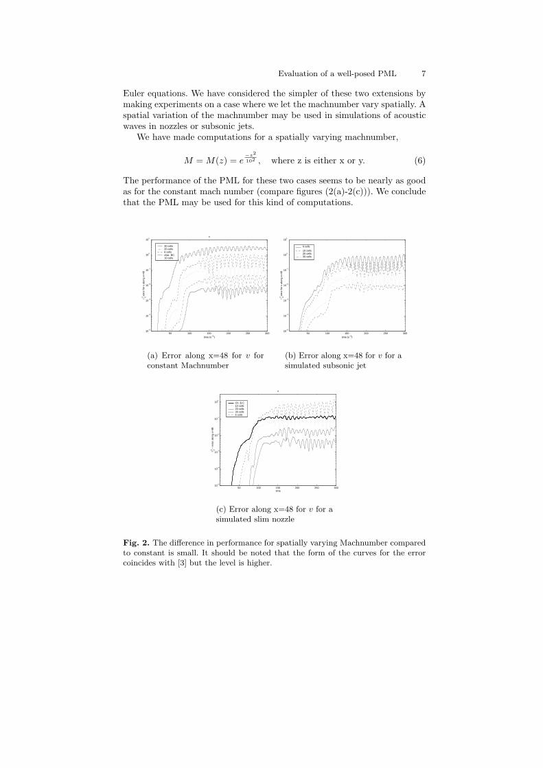
Evaluation of a well-posed PML 7
Euler equations. We have considered the simpler of these two extensions bymaking experiments on a case where we let the machnumber vary spatially. Aspatial variation of the machnumber may be used in simulations of acousticwaves in nozzles or subsonic jets.
We have made computations for a spatially varying machnumber,
M = M(z) = e−z2
102 , where z is either x or y. (6)
The performance of the PML for these two cases seems to be nearly as goodas for the constant mach number (compare figures (2(a)-2(c))). We concludethat the PML may be used for this kind of computations.
50 100 150 200 250 30010
−5
10−4
10−3
10−2
10−1
100
101
v
time [s−1]
l 22 err
or fo
r v
alon
g x=
48
30 cells 20 cells 6 cells char. BC.10 cells
(a) Error along x=48 for v forconstant Machnumber
50 100 150 200 250 30010
−5
10−4
10−3
10−2
10−1
100
101
time [s−1]
l 2 2 err
or fo
r v
alon
g x=
48
6 cells
10 cells20 cells30 cells
(b) Error along x=48 for v for asimulated subsonic jet
50 100 150 200 250 30010
−5
10−4
10−3
10−2
10−1
100
v
time
l 2 2 − e
rror
alo
ng x
=48
Ch. B.C 10 cells20 cells30 cells6 cells
(c) Error along x=48 for v for asimulated slim nozzle
Fig. 2. The difference in performance for spatially varying Machnumber comparedto constant is small. It should be noted that the form of the curves for the errorcoincides with [3] but the level is higher.

8 Daniel Appelo and Gunilla Kreiss
4.2 Efficiency for different waves
We used zero as initial condition for testproblem 2. To avoid transient noisethe solution was first integrated in time for 100 periods. After that the solu-tion was integrated and saved for another period.
Fourier transforming and wavesplitting. To compare different numer-ical solutions we use the Fourier transform in time and in the y-direction.We then use the wavesplitting technique (described above) to extract sepa-rate information on each of the waves of the solution. For each node in thex-direction the amplitude of the other two waves (which ideally should bezero) gives an estimate of the relative error in the computed solution.
In figures 4(a) - 5(b) some examples are shown. We like to stress that inall tests the upstream soundwave amplitude should be taken as the significantestimate of the performance of the absorbing boundary condition since it isthe only one which is reflected from the PML. The other wave is due to theboundary treatment at the inflow boundary.
The results in figures 3(a) and 3(b) show that the PML performs bestfor waves which fall in normal to the outflow boundary. For soundwaves theperformance deteriorates as the angle of incidence decreases. Surprisingly forvorticity waves the worst performance is found at an angle of 60 degrees.However the efficiency of the PML for different angles is always better thancharacteristic boundary conditions.
References
1. S. Abarbanel and D. Gottlieb. A mathematical analysis of the pml method. J.Comput. Phys., 134:357, 1997.
2. S. Abarbanel and D. Gottlieb. On the construction and analysis of absorbinglayers in cem. Appl. Numer. Math., 27:331, 1998.
3. S. Abarbanel, D. Gottlieb, and J.S Hesthaven. Well-posed perfectly matchedlayers for advective acoustics. Journal of Computational Physics, 154:266–283,1999.
4. A. Bayliss and E. Turkel. Radiation boundary conditions for wave-like equa-tions. Comm. Pure Appl. Math., 33:707, 1980.
5. J. P. Brernger. A perfectly matched layer for the absorption of electromagneticwaves. Journal of Computational Physics, 114:185, 1994.
6. B. Engquist and A. Majda. Absorbing boundary conditions for the numericalsimulation of waves. Math. Comp., 31:629, 1977.
7. Wilson. A. G. Method for deriving tone noise information from cfd calculationson the aeroengine fan stage. draft paper, RollsRoyce plc, United Kingdom,2000.
8. Thomas Hagstrom. Radiation boundary conditions for the numerical simulationof waves. Acta Numerica, pages 47–106, 1999.
9. J.S. Hesthaven. On the analysis and construction of perfectly matched layers forthe linearized euler equations. Journal of computational Physics, 142:129–147,1998.

Evaluation of a well-posed PML 9
0 10 20 30 40 50 60 70 80 9010
−6
10−5
10−4
10−3
10−2
10−1
100
Wave direction
Rel
ativ
e er
ror
Ch. b.c. upstream Ch. b.c. vorticityPML upstream PML vorticity
(a) Downstream soundwave. Thecurves display the mean relative er-ror for the vorticity and upstreamsoundwave. Note that the PML isbetter than ch. b.c. for all angles ex-cept for almost glancing incidencewhere the ch. b.c. seems to performas well.
0 10 20 30 40 50 60 70 80 9010
−6
10−5
10−4
10−3
10−2
10−1
100
Wave direction
Rel
ativ
e er
ror
Ch. b.c. downstream Ch. b.c. upstream PML downstream PML upstream
(b) Vorticity wave. Mean relativeerror for the vorticity and upstreamsoundwave. For this type of inflowb.c. the PML is better at all angles.
Fig. 3. The comparison between vorticity and soundwaves show that the PMLwork better for the soundwaves since the vorticity waves has a dip in performanceat 60 degree. The error displayed on the y-axis is the mean error over all x-nodesin the computational domain.
10. F. Q. Hu. On absorbing boundary conditions for linearized euler equations by aperfectly matched layer. Journal of Computational Physics, 129:201–209, 1996.
11. Kristoffer Jensen and Gunilla Efraimsson. Aeroengine fan-noise resolution re-quirement in computational fluid dynamics. Technical report, Swedish Defenceresearch agency, FOI, 2001.

10 Daniel Appelo and Gunilla Kreiss
5 10 15 20 25
10−6
10−5
10−4
10−3
10−2
10−1
100
Nodal number
Nor
mal
ized
am
plitu
de
Exact vorticity amplitude Characteristic b.c. downstream amplitude Characteristic b.c. upstream amplitude Characteristic b.c. vorticity amplitude PML downstream amplitude PML upstream amplitude PML vorticity amplitude
(a) Vorticity wave incoming at an-gle 5.7 degree (almost glancing in-cidence).
5 10 15 20 25
10−6
10−5
10−4
10−3
10−2
10−1
100
Nodal number
Nor
mal
ized
am
plitu
de
Characteristic b.c. downstream amplitudeCharacteristic b.c. upstream amplitude Characteristic b.c. vorticity amplitude PML downstream amplitude PML upstream amplitude PML vorticity amplitude Exact vorticity amplitude
(b) Vorticity wave incoming at an-gle 87.7 degree (almost normal inci-dence).
Fig. 4. Comparison between PML and characteristic boundary condition for a Vor-ticity wave along the computational domain. Note that both boundary conditionswork best at normal incidence.
5 10 15 20 25
10−6
10−5
10−4
10−3
10−2
10−1
100
Nodal number
Nor
mal
ized
am
plitu
de
Exact downstream amplitude Characteristic b.c. downstream amplitudeCharacteristic b.c. upstream amplitude Characteristic b.c.vorticity amplitude PML downstream amplitude PML upstream amplitude PML Vorticity amplitude
(a) Downstream soundwave incom-ing at angle 4.4 degree (almostglancing incidence).
5 10 15 20 25
10−6
10−5
10−4
10−3
10−2
10−1
100
Nodal number
Nor
mal
ized
am
plitu
de
PML downstream amplitude PML upstream amplitude PML vorticity amplitude Characteristic b.c. downstream amplitudeCharacteristic b.c. upstream amplitude Characteristic b.c. vorticity amplitude Exact downstream amplitude
(b) Downstream soundwave incom-ing at angle 86.6 degree (almostnormal incidence)
Fig. 5. Comparison between PML and characteristic boundary condition for adownstream soundwave. Note that both boundary conditions work best at normalincidence.
Department of Numerical Analysis and Computer ScienceTRITA-NA-0325 • ISSN 0348-2952 • ISRN KTH/NA/R--03/25--SE
Stabilized Local Non-reflectingBoundary Conditions for High
Order Methods
Daniel Appelö and Gunilla Kreiss
Numerical Analysis
Daniel Appelö and Gunilla KreissStabilized Local Non-reflecting Boundary Conditions for High Order Methods
Report number: TRITA-NA-0325, ISRN KTH/NA/R--03/25--SEPublication date: November 2003E-mail of author: [email protected]
Department of Numerical Analysis and Computer ScienceRoyal Institute of TechnologySE-100 44 StockholmSWEDEN

Abstract
Using the framework introduced by Rowley and Colonius [14] we construct a dis-cretely non-reflecting boundary condition for the one-way wave equation spatiallydiscretized with an explicit fourth order centered difference scheme. The boundarycondition, which can be extended to arbitrary order accuracy, is shown to be GKS-stable. We continue by deriving discretely non-reflecting boundary conditions forsystems in two dimensions using the results for the scalar one dimensional case.
TRITA-NA-0325 • ISSN 0348-2952 • ISRN KTH/NA/R--03/25--SE
3

4
1 Introduction
When solving hyperbolic problems numerically on unbounded domains, the problemis confined to a smaller computational domain by introducing an artificial boundary.For many hyperbolic problems the correct boundary condition is that waves travel-ing across the boundary should not be reflected back. Boundary conditions whichprevent waves from being reflected are often referred to as non-reflecting boundaryconditions. Sometimes they may be referred to as transparent, artificial or absorbingboundary conditions.
Non-reflecting boundary conditions have been a matter of research for manydecades. Some early explorers of the area were Lindeman [13] and Engquist andMajda [4], [5], who derived non-reflecting boundary conditions for the scalar waveequation. The works of Engquist and Majda have been an important source ofinspiration in the construction of non-reflecting boundary conditions in differentfields.
Boundary conditions of Engquist - Majda type are often formulated as a se-quence of partial differential equations (PDE) which do not allow waves to travelback into the computational domain. The boundary conditions can be of differentorder, where a high order is equivalent with high order derivatives in the PDEs gov-erning the boundary condition. When using such boundary conditions in numericalcomputations some possible drawbacks become apparent. The first is the questionof how to discretize the high order (mixed) derivatives in a stable fashion. A wayto handle this problem is to introduce auxiliary variables such that a system of firstorder PDEs is solved instead of the high order PDE on the boundary. However theissue of a stable discretization may still be present, especially when using numericalmethods of high order. The second possible drawback relates to the fact that whenany discretization procedure is used, spurious non-physical solutions are introduced.Boundary conditions which are non-reflecting for physical solutions may be highlyreflective for its spurious counterpart. This indicates that it may be fruitful to con-sider discretely non-reflecting boundary conditions i.e. boundary conditions whichare non-reflecting for both physical and spurious solutions.
The construction of a discretely non-reflecting boundary condition depends onthe discretization procedure used, i.e. for each specific scheme a new boundarycondition must be derived. In this paper we present the construction of a discretelynon-reflecting boundary condition for the one-way wave equation where the standardfive-point central difference approximation is used for the first order derivative inspace.
In the recent paper [14] Rowley and Colonius have provided a framework forsuch construction. They construct boundary conditions for an implicit Padé three-point central difference scheme to illustrate their analysis. The discrete boundaryconditions are then used to construct boundary conditions for the linearized Eulerequations in two dimensions.
We consider a simpler model problem for the extension of our discrete scalarboundary condition to systems in two dimensions. The ideas presented here are
5

directly applicable to any hyperbolic problem in two dimensions.The Padé scheme, used in [14], is a fourth order implicit scheme. Widening the
stencil from three to five points allows for an explicit fourth order scheme. Howeverthe issue of stability of the boundary condition becomes more involved.
The boundary conditions is extended to two space dimensions by combining exactcontinuous non-reflecting boundary conditions and the one dimensional discretelynon-reflecting boundary condition. The resulting boundary condition is localized bythe standard Padé approximation. By using auxiliary variables the two dimensionalboundary condition can, in principal , be extended to high-order. However it isfound by numerical experiments that the resulting method suffers from boundaryinstabilities.
Analysis of a related continuous problem suggests that the discrete boundarycondition can be stabilized by adding tangential viscosity at the boundary. For thelowest order Padé approximation we are able to stabilize the discrete boundary con-dition. However, the results of the stabilized boundary condition is not satisfactory.The reflections are smaller than for the standard boundary condition but does notmotivate the extra work needed to implement them.
2 Discretely Non-Reflecting Boundary Conditions in oneDimension
When solving hyperbolic problems with numerical methods, it is preferred to useexplicit methods both in time and space. For truncated problems, the geometries ofthe outer boundary can often be chosen as preferred, e.g. as a box. For such simplegeometry, the obvious choice of discretization is centered differences of high orderin space combined with an explicit high order method (e.g. Runge-Kutta) in time.This combination yields an easy to implement, accurate and fast numerical method.By using centered differences in space and assuming that the grid is regular, at leastclose to the boundary, the errors produced by spurious waves may be controlled andminimized by discrete analysis.
In section 2.1 we recall some basic facts of finite difference schemes for hyperbolicproblems. The notation of physical and spurious waves are introduced together withthe discrete group and phase velocity.
In sections 2.2-2.3 we construct approximate discretely non-reflecting boundaryconditions such that reflections caused by the coupling of spurious and physicalmodes are minimized.
2.1 Spurious and Physical Waves in One Dimensional Finite Dif-ference Schemes
We begin by considering the scalar one-way wave equation
ut + ux = 0, (1)
6

which admits solutions on the form
u(x, t) = ei(kx−ωt). (2)
Inserting (2) into (1), we obtain the dispersion relation ω ≡ ω(k) = k, where k isthe wave number and ω the frequency. For an equation with a dispersion relation,the phase velocity, cp, and group velocity, cg can be defined as
cp =ω(k)k
, cg =dω(k)dk
.
For the equation (1), cp = cg = 1.
Discrete Dispersion Relation
It is well known (see [16] for a detailed discussion) that a discretization of (1) willaffect the dispersion relation and thereby the phase and group velocity. Differentschemes have different dispersion relations and therefore they have to be analyzedseparately.
In [14], Colonius and Rowley analyze a fourth order accurate, compact centeredthree point difference scheme. The advantage of using a compact three point schemeis that only one type of spurious waves will appear. The main disadvantage isthat the scheme is implicit. Here, we will analyze the standard centered five pointdifference scheme of order four.
We start by introducing a regular grid in x, with mesh spacing h. Let uk denotethe approximation of u(xk) where xk = kh and k = 0, 1, . . . , N . We use the centralfinite difference approximation
∂u(xk)∂x
≈ 112h
(−uk+2 + 8uk+1 − 8uk−1 + uk−2). (3)
of ux in(1) and obtain
(ut)k =1
12h(uk+2 − 8uk+1 + 8uk−1 − uk−2). (4)
The dispersion relation of (4) is
ω(k) =43h
sin kh− 16h
sin 2kh
In Figure 1 we compare dispersion relations and group velocities for the continuousproblem and the discretized problem. Note that poorly resolved waves (kh ≈ π)travel in the opposite direction, i.e. cg < 0, to well resolved waves.
In Figure 1 (a) we can also see that for each frequency ω(k), there are two valuesof k that satisfy the dispersion relation. The smaller one corresponds to a physicalwave and the larger one corresponds to a spurious wave. For three point schemes,these two waves are the only type of waves that exist but for the fourth order scheme
7

0 0.1 0.2 0.3 0.4 0.5 0.6 0.7 0.8 0.9 10
0.1
0.2
0.3
0.4
0.5
0.6
0.7
0.8
0.9
1
kh / π
ω h
/ π
ωcont
ω2
ω4
ωpade
(a) Dispersion relations for different disc-tretizations.
0 0.1 0.2 0.3 0.4 0.5 0.6 0.7 0.8 0.9 1
−3
−2.5
−2
−1.5
−1
−0.5
0
0.5
1
kh / π
c g
cg cont
cg 2
cg 4
cg Pade
(b) Group velocities for different disc-tretizations.
Figure 1. The notation ωcont, ω2, ω4and ωPade refers to the continuous, standard2nd order centered scheme, standard 4th order scheme and the compact scheme [14].
u*u/
u+
u−
Figure 2. Different types of waves supported by standard five point centered dif-ference scheme. u+ corresponds to a physical right-going wave, u− to a spuriousleft-going wave, u∗ to a spurious wave decaying from the left and u÷ to a spuriouswave decaying from the right.
8
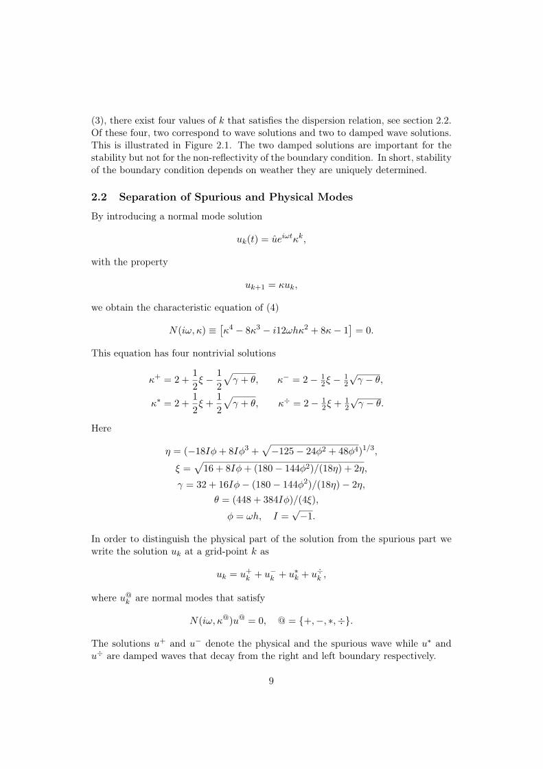
(3), there exist four values of k that satisfies the dispersion relation, see section 2.2.Of these four, two correspond to wave solutions and two to damped wave solutions.This is illustrated in Figure 2.1. The two damped solutions are important for thestability but not for the non-reflectivity of the boundary condition. In short, stabilityof the boundary condition depends on weather they are uniquely determined.
2.2 Separation of Spurious and Physical Modes
By introducing a normal mode solution
uk(t) = ueiωtκk,
with the property
uk+1 = κuk,
we obtain the characteristic equation of (4)
N(iω, κ) ≡ [κ4 − 8κ3 − i12ωhκ2 + 8κ− 1
]= 0.
This equation has four nontrivial solutions
κ+ = 2 +12ξ − 1
2
√γ + θ, κ− = 2− 1
2ξ − 12
√γ − θ,
κ∗ = 2 +12ξ +
12
√γ + θ, κ÷ = 2− 1
2ξ + 12
√γ − θ.
Here
η = (−18Iφ+ 8Iφ3 +√−125− 24φ2 + 48φ4)1/3,
ξ =√
16 + 8Iφ+ (180− 144φ2)/(18η) + 2η,
γ = 32 + 16Iφ− (180− 144φ2)/(18η)− 2η,θ = (448 + 384Iφ)/(4ξ),
φ = ωh, I =√−1.
In order to distinguish the physical part of the solution from the spurious part wewrite the solution uk at a grid-point k as
uk = u+k + u−k + u∗k + u÷k ,
where u@k are normal modes that satisfy
N(iω, κ@)u@ = 0, @ = +,−, ∗,÷.
The solutions u+ and u− denote the physical and the spurious wave while u∗ andu÷ are damped waves that decay from the right and left boundary respectively.
9

2.3 Approximate Non-Reflecting Boundary Conditions
We now seek approximate non-reflecting boundary conditions at the left (k = 0) andat the right (k = N) boundary. Following the ideas of Colonius [2] and Coloniusand Rowley [14] we seek approximate boundary conditions of the form
du0
dt=
1c1h
Nd∑
k=0
dkuk ≡ di0u0,
duN
dt=
1a1h
Nd∑
k=0
bkuN−k ≡ doNuN , (5)
where a1, bk, c1, dk, (k = 0, . . . , Nd) are coefficients to be determined. Here Nd isthe order of the boundary condition. Consider first the left boundary.
Taking the Fourier transform in time and splitting u into its different modes, (5)becomes
ic1ωh(u+0 + u−0 + u∗0 + u÷0 ) =
Nd∑
k=0
dk(u+k + u−k + u∗k + u÷k )
⇐⇒ ic1ωhu+0 −
Nd∑
k=0
dk(κ+)ku+0 =
−ic1ωh(u−0 + u∗0 + u÷0 ) +Nd∑
k=0
dk
[(κ−)ku−0 + (κ∗)ku∗0 + (κ÷)ku÷0
].
(6)
With φ = ωh, (6) becomes
d+(φ)u+0 = d−(φ)u−0 + d∗(φ)u∗0 + d÷(φ)u÷0 ,
where
d+(φ) = c1iφ−Nd∑
k=0
dk(κ+)k,
d@(φ) = −c1iφ+Nd∑
k=0
dk(κ@)k, @ = −, ∗,÷.
The exact non-reflecting boundary condition, u+0 = 0, would be satisfied if
d@(φ) = 0, @ = −, ∗,÷.
It is not possible to fulfill d@(φ) = 0 for all @ = −, ∗,÷. However this is notnecessary since u÷ will be eliminated later and u∗ must be specified at the rightboundary and will be very small at the left boundary. Thus only d−(φ) = 0 remains,this is equivalent with the condition obtained in [14].
Since d−(φ) contains powers of κ− up to order Nd, it is natural to expand κ−(φ)as a power series expansion around φ = 0. The coefficients c1, d0, . . . are chosen suchthat d−(φ) is minimized.
10

At the right boundary we use the same technique to find the boundary conditionfor uN . Separating the spurious and physical modes of the ansatz (5) leads to thefollowing expression
b+(φ)u+N = b−(φ)u−N + b∗(φ)u∗N + b÷(φ)u÷N ,
where
b+(φ) = ac1iφ−Nd∑
k=0
bk(κ+)k
,
b@(φ) = −a1iφ+Nd∑
k=0
bk(κ@)k
, @ = −, ∗,÷.
The non-reflecting boundary condition for uN is b+(φ) = 0. For an equation with aleft-going physical solution, e.g vt − vx = 0, the analysis is similar. The role of thespurious and physical solution at a boundary will be the opposite compared to anequation with a right-going physical solution. Using the notation introduced in (5),we may write boundary closures for the equation vt − vx = 0 as
dv0dx
= do0v0,
dvN
dx= di
NvN .
2.4 Stability
When applying the scheme (3) to the gridpoint k = 1 we need information of bothu0 and u−1. Above, u0 has been determined to minimize the reflection at k = 0. Therelation determining u−1 must be chosen such that the boundary condition is stable.The mathematically correct boundary condition is u(t, 0) = 0, which together with(1) gives the relation u(t, 0)xx = 0. First consider a three point wide stencil for theapproximation of (uxx)k=0, which yield the relation
u−1 = 2u0 − u1. (7)
It can be shown that (7) yields a stable boundary condition for choices of Nd atleast up to Nd = 8. For example, consider Nd = 1 which gives the following relationfor u0
du0
dt= − 5
3h(u0 + u1). (8)
To investigate the stability of the above boundary conditions for (4) we use Laplacetransform technique (see e.g. [9]). We obtain the following eigenvalue problem
sψj =1
12h(ψj+2 − 8ψj+1 + 8ψj−1 − ψj−2), s = sh. (9)
11
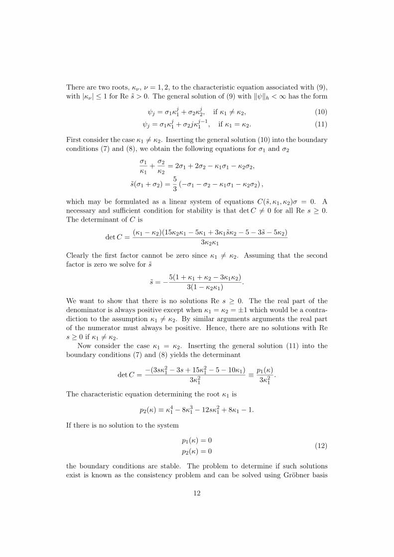
There are two roots, κν , ν = 1, 2, to the characteristic equation associated with (9),with |κν | ≤ 1 for Re s > 0. The general solution of (9) with ‖ψ‖h <∞ has the form
ψj = σ1κj1 + σ2κ
j2, if κ1 6= κ2, (10)
ψj = σ1κj1 + σ2jκ
j−11 , if κ1 = κ2. (11)
First consider the case κ1 6= κ2. Inserting the general solution (10) into the boundaryconditions (7) and (8), we obtain the following equations for σ1 and σ2
σ1
κ1+σ2
κ2= 2σ1 + 2σ2 − κ1σ1 − κ2σ2,
s(σ1 + σ2) =53
(−σ1 − σ2 − κ1σ1 − κ2σ2) ,
which may be formulated as a linear system of equations C(s, κ1, κ2)σ = 0. Anecessary and sufficient condition for stability is that detC 6= 0 for all Re s ≥ 0.The determinant of C is
detC =(κ1 − κ2)(15κ2κ1 − 5κ1 + 3κ1sκ2 − 5− 3s− 5κ2)
3κ2κ1
Clearly the first factor cannot be zero since κ1 6= κ2. Assuming that the secondfactor is zero we solve for s
s = −5(1 + κ1 + κ2 − 3κ1κ2)3(1− κ2κ1)
.
We want to show that there is no solutions Re s ≥ 0. The the real part of thedenominator is always positive except when κ1 = κ2 = ±1 which would be a contra-diction to the assumption κ1 6= κ2. By similar arguments arguments the real partof the numerator must always be positive. Hence, there are no solutions with Res ≥ 0 if κ1 6= κ2.
Now consider the case κ1 = κ2. Inserting the general solution (11) into theboundary conditions (7) and (8) yields the determinant
detC =−(3sκ2
1 − 3s+ 15κ21 − 5− 10κ1)
3κ21
≡ p1(κ)3κ2
1
.
The characteristic equation determining the root κ1 is
p2(κ) ≡ κ41 − 8κ3
1 − 12sκ21 + 8κ1 − 1.
If there is no solution to the system
p1(κ) = 0p2(κ) = 0
(12)
the boundary conditions are stable. The problem to determine if such solutionsexist is known as the consistency problem and can be solved using Gröbner basis
12

0 10 20 30 40 50 60 70 80 90 100−1
−0.5
0
0.5
1
High frequency initial data
u(x)
0 10 20 30 40 50 60 70 80 90 100−1
−0.5
0
0.5
1
Low frequency initial data
u(x)
Figure 3. Initial data for experiments in one dimension.
[3]. Using the symbolic software Maple we are able to determine that there are nosolutions to the system (12), hence the boundary conditions are stable.
Note that the boundary condition (7) is only second order which would degradethe overall accuracy of the method if used. Instead of (7) we use the fourth orderaccurate, five point, skew approximation of uxx which also will yield a stable bound-ary condition. Since this approximation is used, the overall order of the method willbe four.
For the right boundary, a skew difference stencil Dq−uN−1 together with the
non-reflective boundary conditions derived above can be shown to yield a stableboundary condition. If q is chosen large enough the over all order of accuracy willbe four.
2.5 Numerical experiments in 1D
To test the boundary condition, we consider the one-way wave equation (1) on thecomputational domain x ∈ [0, 100], discretized with a regular grid. The spatialderivative is approximated by using the fourth order stencil (3) terminated usingthe discretely non-reflecting boundary conditions discussed in the previous section.The integration in time is performed with the standard fourth order Runge Kuttamethod. As a comparison, we use characteristic boundary conditions, i.e. u(0, t) =0, together with extrapolation at the right boundary. The error is computed usinga reference solution computed on a larger domain.
The boundary conditions are tested for two sets of initial data u(x, 0)
uhigh(xk) = (−1)ku(xk),ulow(xk) = u(xk),
u(x) = e−(x−50)2
102 .
13

The initial data uhigh is oscillating with the highest frequency allowed on the gridwhile the initial data ulow is smooth, see Figure 3. In Figure 4 the error for different
0 10 20 30 40 50 6010
−20
10−18
10−16
10−14
10−12
10−10
10−8
norm
(err
or)/
norm
(initi
al d
ata)
time
standard234567
(a) The l2 error on the computational do-main for the smooth initial data for dif-ferent Nd compared with characteristicboundary conditions. For Nd > 4 the dis-cretely non-reflecting boundary conditionoutperforms the characteristic boundarycondition.
0 10 20 30 40 50 6010
−6
10−5
10−4
10−3
10−2
norm
(err
or)/
norm
(initi
al d
ata)
time
standard234567
(b) The l2 error on the computational do-main for the non-smooth initial data fordifferent Nd compared with characteristicboundary conditions. Here the discretelynon-reflecting boundary condition is moreefficient then characteristic boundary con-ditions for all Nd.
Figure 4.
Nd is compared to the error introduced by characteristic boundary conditions. It isclear that for large Nd, the discretely non-reflecting boundary conditions are moreefficient than characteristic boundary conditions independent of the smoothness ofthe initial data. Especially for the non-smooth initial data, the discretely non-reflecting boundary condition works well.
3 Continuous Non-Reflecting Boundary Conditions
An important feature of linear systems of hyperbolic equations is that it is possible toseparate in-going and out-going parts of the solution at a boundary. The decomposi-tion of the solution at a boundary is obtained by using the theory of characteristics.This decomposition of the solution is closely related to the well-posedness of theproblem. The necessary condition for well-posedness is that in-going components ofthe solution must be specified by the boundary conditions at each boundary.
If the boundary condition is to be well-posed and non-reflecting, the in-goingmodes should be put to zero. This will prevent reflection of the solution back intothe domain. Below, we construct well-posed, non-reflecting boundary conditions fora simple model problem in two dimensions. For a complete discussion of construction
14
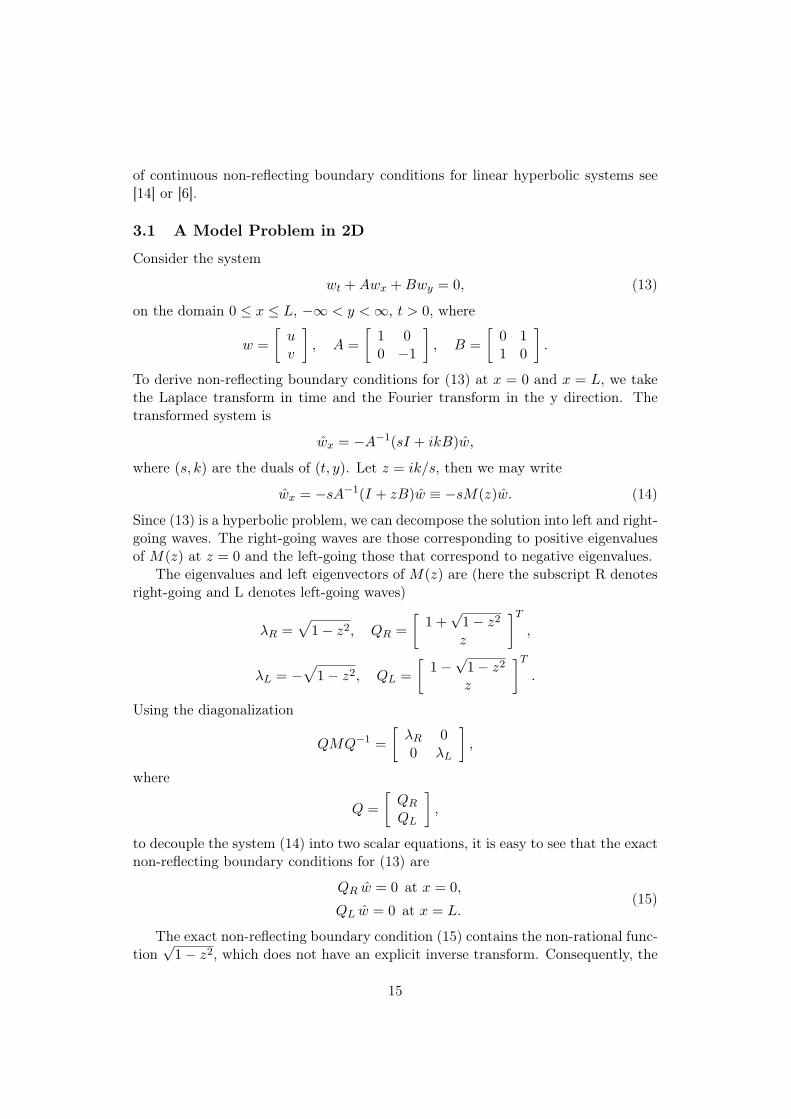
of continuous non-reflecting boundary conditions for linear hyperbolic systems see[14] or [6].
3.1 A Model Problem in 2D
Consider the system
wt +Awx +Bwy = 0, (13)
on the domain 0 ≤ x ≤ L, −∞ < y <∞, t > 0, where
w =[uv
], A =
[1 00 −1
], B =
[0 11 0
].
To derive non-reflecting boundary conditions for (13) at x = 0 and x = L, we takethe Laplace transform in time and the Fourier transform in the y direction. Thetransformed system is
wx = −A−1(sI + ikB)w,
where (s, k) are the duals of (t, y). Let z = ik/s, then we may write
wx = −sA−1(I + zB)w ≡ −sM(z)w. (14)
Since (13) is a hyperbolic problem, we can decompose the solution into left and right-going waves. The right-going waves are those corresponding to positive eigenvaluesof M(z) at z = 0 and the left-going those that correspond to negative eigenvalues.
The eigenvalues and left eigenvectors of M(z) are (here the subscript R denotesright-going and L denotes left-going waves)
λR =√
1− z2, QR =[
1 +√
1− z2
z
]T
,
λL = −√
1− z2, QL =[
1−√1− z2
z
]T
.
Using the diagonalization
QMQ−1 =[λR 00 λL
],
where
Q =[QR
QL
],
to decouple the system (14) into two scalar equations, it is easy to see that the exactnon-reflecting boundary conditions for (13) are
QR w = 0 at x = 0,
QL w = 0 at x = L.(15)
The exact non-reflecting boundary condition (15) contains the non-rational func-tion
√1− z2, which does not have an explicit inverse transform. Consequently, the
15

corresponding boundary condition in the physical space will be exact but nonlocal intime and space. This non locality is undesirable and leads to expensive and cumber-some implementation of the boundary conditions when used for computations. Tolocalize these boundary conditions,
√1− z2 may e.g. be replaced by some rational
approximant, which can be transformed back directly.
3.2 Rational Approximants and Non-Reflecting Boundary Condi-tions
The problem of approximating the function√
1− z2 in the context of non-reflectingboundary conditions has been extensively studied in the literature. See e.g. Engquistand Majda [4]. Trefethen and Halpern [15] provides detailed studies of different typeof approximations (Padé, Chebyshev and least-squares).
In this paper we consider only the Padé approximations which yield well-posed,see [15], boundary conditions in exactly the diagonals, m = n and m = n+ 2 of thetable of approximants (m,n).
By replacing√
1− z2 with the Padé approximant, in QR and QL, we obtain thefollowing approximate non-reflecting boundary conditions
ER w = 0 at x = 0,
EL w = 0 at x = L.(16)
4 Discretely Non-Reflecting Boundary Conditions in 2D
To derive a discretely non-reflecting boundary condition in two dimensions, we canuse the exact boundary conditions, discussed in section 3.1, together with the dis-cretely non-reflecting boundary conditions discussed in section 2.3. Since the dis-cretely non-reflecting boundary conditions are directly applicable for one-way equa-tions we use the exact continuous boundary conditions for (13) to obtain one-wayequations.
Consider again the transformed version of the system (13)
wx = −sM(z)w, (17)
with the exact non-reflecting boundary conditions (15)
QR w = 0 at x = 0,
QL w = 0 at x = L.
Now define the matrix
Q(z) =[QR
QL
],
and let T (z) be the matrix composed by the right eigenvectors to M(z) such that
T−1MT =[λR 00 λL
]≡ Λ. (18)
16
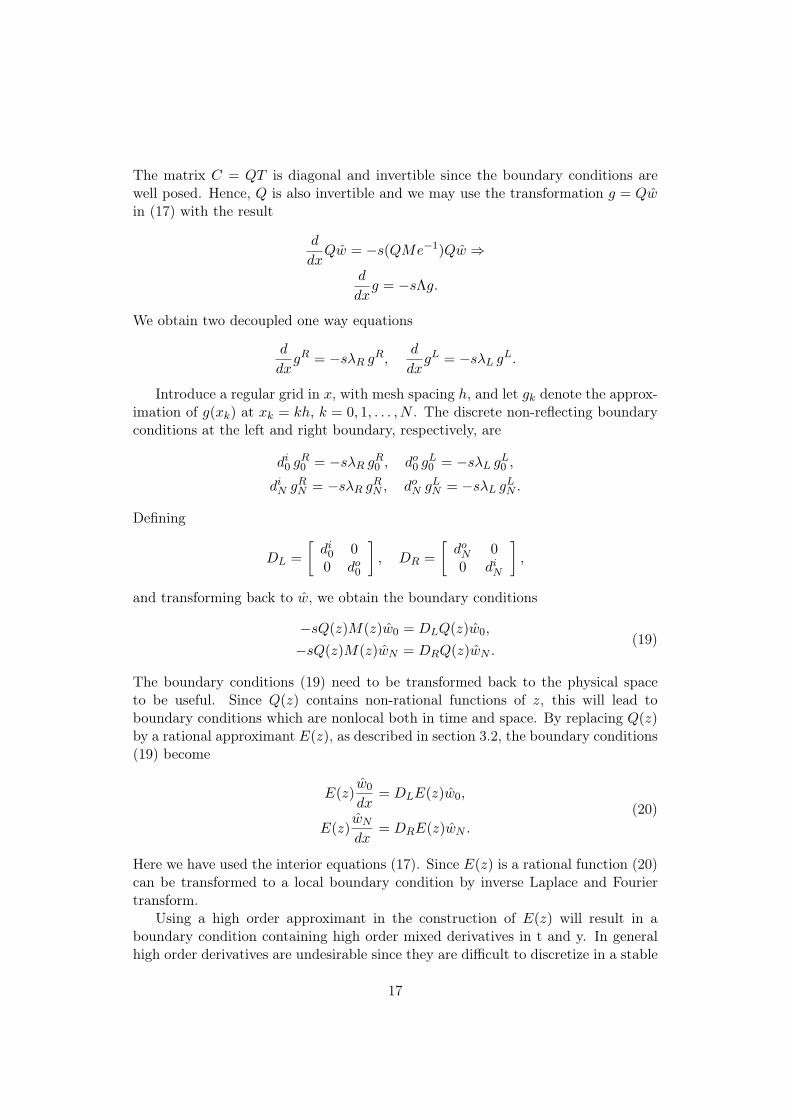
The matrix C = QT is diagonal and invertible since the boundary conditions arewell posed. Hence, Q is also invertible and we may use the transformation g = Qwin (17) with the result
d
dxQw = −s(QMe−1)Qw ⇒
d
dxg = −sΛg.
We obtain two decoupled one way equations
d
dxgR = −sλR g
R,d
dxgL = −sλL g
L.
Introduce a regular grid in x, with mesh spacing h, and let gk denote the approx-imation of g(xk) at xk = kh, k = 0, 1, . . . , N . The discrete non-reflecting boundaryconditions at the left and right boundary, respectively, are
di0 g
R0 = −sλR g
R0 , do
0 gL0 = −sλL g
L0 ,
diN gR
N = −sλR gRN , do
N gLN = −sλL g
LN .
Defining
DL =[di
0 00 do
0
], DR =
[do
N 00 di
N
],
and transforming back to w, we obtain the boundary conditions
−sQ(z)M(z)w0 = DLQ(z)w0,
−sQ(z)M(z)wN = DRQ(z)wN .(19)
The boundary conditions (19) need to be transformed back to the physical spaceto be useful. Since Q(z) contains non-rational functions of z, this will lead toboundary conditions which are nonlocal both in time and space. By replacing Q(z)by a rational approximant E(z), as described in section 3.2, the boundary conditions(19) become
E(z)w0
dx= DLE(z)w0,
E(z)wN
dx= DRE(z)wN .
(20)
Here we have used the interior equations (17). Since E(z) is a rational function (20)can be transformed to a local boundary condition by inverse Laplace and Fouriertransform.
Using a high order approximant in the construction of E(z) will result in aboundary condition containing high order mixed derivatives in t and y. In generalhigh order derivatives are undesirable since they are difficult to discretize in a stable
17

and accurate manner. Especially, this is true when using a high order scheme in theinterior.
To obtain boundary conditions containing no mixed derivatives, auxiliary vari-ables may be introduced. These variables can be chosen in many ways. Here wechose the approach suggested in Rowley and Colonius [14]. Alternative approachescan be found in e.g. Hagstrom and Harihan [8] or Givoli and Neta [7].
4.1 Non-Reflecting Boundary Conditions using Auxiliary Variables
We start by multiplying each row of equation (20) by its least common denominatorto obtain the following system
E′(z)w0
dx= DLE
′(z)w0, (21)
E′(z)wN
dx= DRE
′(z)wN , (22)
where
E′(z) = E0 + zE1 + · · ·+ zpEp.
Introduce auxiliary variables hj such that (21) becomes
E0∂w0
∂x= DLE0w0 +
∂
∂y(F0w0 + h1),
∂hj
∂t= DLEjw0 +
∂
∂y(Fjw0 + hj+1), j = 1, . . . , p− 1
∂hp
∂t= DLEpw0 +
∂
∂y(Fpw0),
(23)
where
F0 = E1A−1,
Fj = EjA−1B +Ej+1A
−1, j = 1, . . . , p− 1
Fp = EpA−1B.
The boundary condition (23) is easy to implement and the extra amount of mem-ory needed for the auxiliary variables is proportional to the order of the rationalapproximant. For the boundary conditions at the right boundary, simply replace w0
by wN .
18
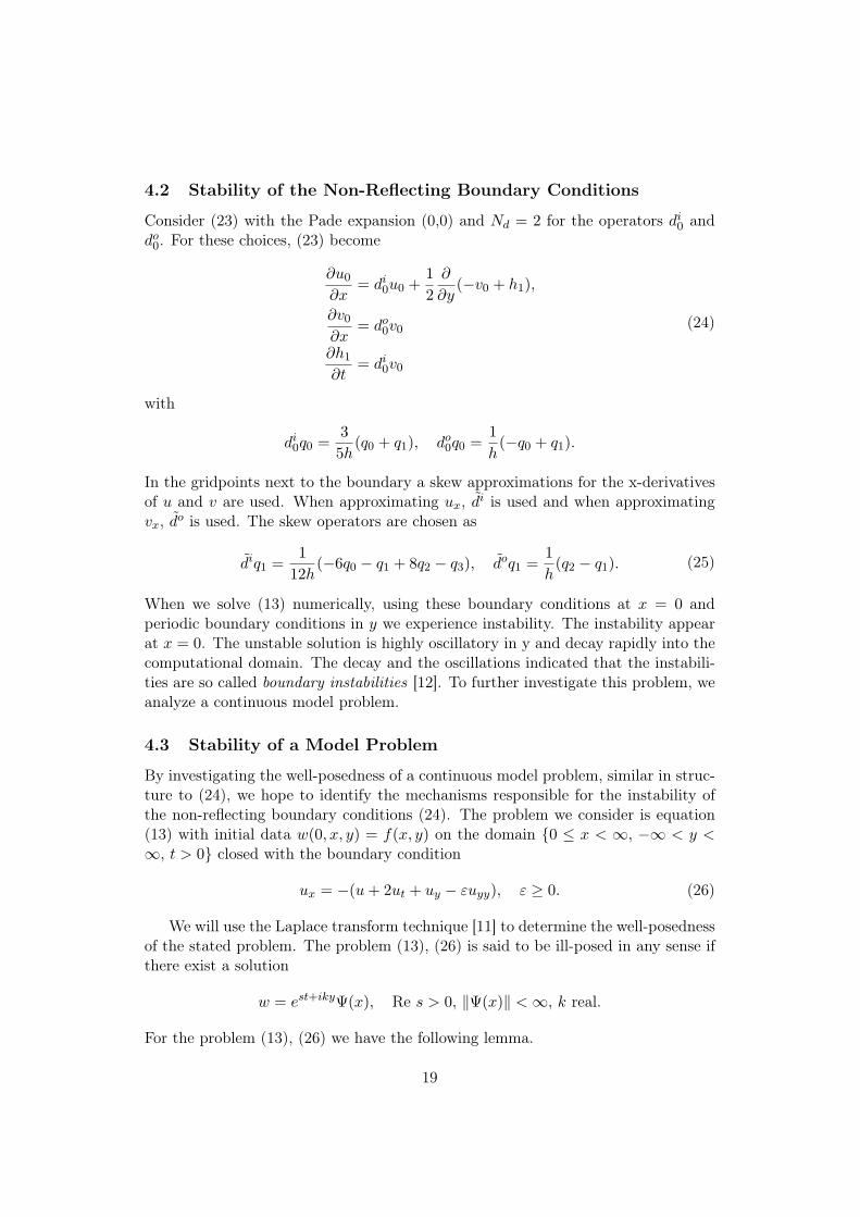
4.2 Stability of the Non-Reflecting Boundary Conditions
Consider (23) with the Pade expansion (0,0) and Nd = 2 for the operators di0 and
do0. For these choices, (23) become
∂u0
∂x= di
0u0 +12∂
∂y(−v0 + h1),
∂v0∂x
= do0v0
∂h1
∂t= di
0v0
(24)
with
di0q0 =
35h
(q0 + q1), do0q0 =
1h
(−q0 + q1).
In the gridpoints next to the boundary a skew approximations for the x-derivativesof u and v are used. When approximating ux, di is used and when approximatingvx, do is used. The skew operators are chosen as
diq1 =1
12h(−6q0 − q1 + 8q2 − q3), doq1 =
1h
(q2 − q1). (25)
When we solve (13) numerically, using these boundary conditions at x = 0 andperiodic boundary conditions in y we experience instability. The instability appearat x = 0. The unstable solution is highly oscillatory in y and decay rapidly into thecomputational domain. The decay and the oscillations indicated that the instabili-ties are so called boundary instabilities [12]. To further investigate this problem, weanalyze a continuous model problem.
4.3 Stability of a Model Problem
By investigating the well-posedness of a continuous model problem, similar in struc-ture to (24), we hope to identify the mechanisms responsible for the instability ofthe non-reflecting boundary conditions (24). The problem we consider is equation(13) with initial data w(0, x, y) = f(x, y) on the domain 0 ≤ x < ∞, −∞ < y <∞, t > 0 closed with the boundary condition
ux = −(u+ 2ut + uy − εuyy), ε ≥ 0. (26)
We will use the Laplace transform technique [11] to determine the well-posednessof the stated problem. The problem (13), (26) is said to be ill-posed in any sense ifthere exist a solution
w = est+ikyΨ(x), Re s > 0, ‖Ψ(x)‖ <∞, k real.
For the problem (13), (26) we have the following lemma.
19
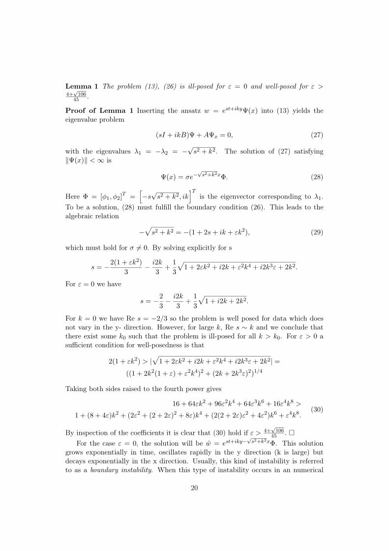
Lemma 1 The problem (13), (26) is ill-posed for ε = 0 and well-posed for ε >4+√
10645 .
Proof of Lemma 1 Inserting the ansatz w = est+ikyΨ(x) into (13) yields theeigenvalue problem
(sI + ikB)Ψ +AΨx = 0, (27)
with the eigenvalues λ1 = −λ2 = −√s2 + k2. The solution of (27) satisfying‖Ψ(x)‖ <∞ is
Ψ(x) = σe−√
s2+k2xΦ. (28)
Here Φ = [φ1, φ2]T =
[−s√s2 + k2, ik
]Tis the eigenvector corresponding to λ1.
To be a solution, (28) must fulfill the boundary condition (26). This leads to thealgebraic relation
−√s2 + k2 = −(1 + 2s+ ik + εk2), (29)
which must hold for σ 6= 0. By solving explicitly for s
s = −2(1 + εk2)3
− i2k3
+13
√1 + 2εk2 + i2k + ε2k4 + i2k3ε+ 2k2.
For ε = 0 we have
s = −23− i2k
3+
13
√1 + i2k + 2k2.
For k = 0 we have Re s = −2/3 so the problem is well posed for data which doesnot vary in the y- direction. However, for large k, Re s ∼ k and we conclude thatthere exist some k0 such that the problem is ill-posed for all k > k0. For ε > 0 asufficient condition for well-posedness is that
2(1 + εk2) > |√
1 + 2εk2 + i2k + ε2k4 + i2k3ε+ 2k2| =((1 + 2k2(1 + ε) + ε2k4)2 + (2k + 2k3ε)2)1/4
Taking both sides raised to the fourth power gives
16 + 64εk2 + 96ε2k4 + 64ε3k6 + 16ε4k8 >
1 + (8 + 4ε)k2 + (2ε2 + (2 + 2ε)2 + 8ε)k4 + (2(2 + 2ε)ε2 + 4ε2)k6 + ε4k8.(30)
By inspection of the coefficients it is clear that (30) hold if ε > 4+√
10645 . ¤
For the case ε = 0, the solution will be w = est+iky−√s2+k2xΦ. This solutiongrows exponentially in time, oscillates rapidly in the y direction (k is large) butdecays exponentially in the x direction. Usually, this kind of instability is referredto as a boundary instability. When this type of instability occurs in an numerical
20

method, the remedy is to add a small number of tangential viscosity to stabilizethe numerical method. The addition of tangential viscosity can be understood bythe above analysis. Since the boundary condition (26) has a structure similar tothe discrete boundary condition (23), it is reasonable to expect that instabilitiesobserved in the numerical computations may be removed by adding a sufficientamount of tangential viscosity.
4.4 Stabilized Non-Reflecting Boundary Condition
We want to add viscosity to stabilize the boundary conditions (24). Viscosity isintroduced by adding the term εvyy to the first row of the equations (13). This isequivalent to modify the the matrix M(z) to
M(z) =[
1 + εk2 z−z −1
].
This modification is used at the two gridpoints next to the boundary.To analyze the stabilized boundary conditions, we use the Laplace transform
technique on the halfplane problem, defined by the equations (13), (24) on 0 ≤x < ∞, −∞ < y < ∞, t > 0. Taking the Fourier transform in y direction andthe Laplace transform in time yield the following relations at the gridpoints xi, i =0, 1, 2
−sE′(z)M(z)w0 = DLE′(z)w0,
−sM(z)w1 = Dw1,
−sM(z)w2 = D(4)w2.
(31)
The first relation contains the non-reflecting boundary condition (24). The secondequation contains the operator D = diag(di, do) defined in (25). The operator D(4)
is the usual fourth order accurate approximation of the derivative and the matrixM(z) is modified as described above.
Away from the boundary, the solution is determined by the equation
−sM(z)wk = D(4)wk, k > 2. (32)
The general solution of (32), satisfying ‖wk‖h <∞, ∀k with Re s > 0, is
wk =[σ+
R(κ+R)k + σ÷R(κ÷R)k
]ΨR(z) +
[σ−L (κ+
L )k + σ∗L(κ∗L)k]ΨL(z). (33)
Here the σ+R , σ
÷R , σ
−L , σ
∗L are constants to be determined by the relations (31). The
subscript L correspond to a left-going mode and R to a right-going. The vectors
21
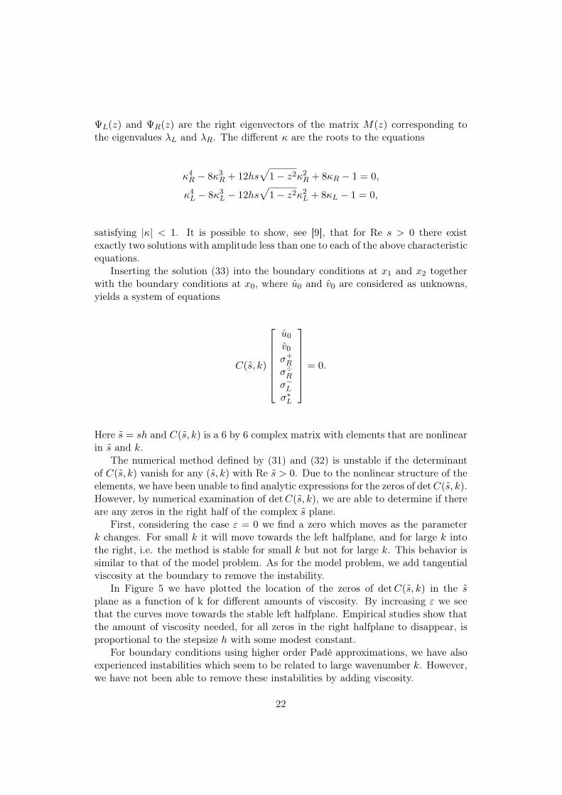
ΨL(z) and ΨR(z) are the right eigenvectors of the matrix M(z) corresponding tothe eigenvalues λL and λR. The different κ are the roots to the equations
κ4R − 8κ3
R + 12hs√
1− z2κ2R + 8κR − 1 = 0,
κ4L − 8κ3
L − 12hs√
1− z2κ2L + 8κL − 1 = 0,
satisfying |κ| < 1. It is possible to show, see [9], that for Re s > 0 there existexactly two solutions with amplitude less than one to each of the above characteristicequations.
Inserting the solution (33) into the boundary conditions at x1 and x2 togetherwith the boundary conditions at x0, where u0 and v0 are considered as unknowns,yields a system of equations
C(s, k)
u0
v0σ+
R
σ÷Rσ−Lσ∗L
= 0.
Here s = sh and C(s, k) is a 6 by 6 complex matrix with elements that are nonlinearin s and k.
The numerical method defined by (31) and (32) is unstable if the determinantof C(s, k) vanish for any (s, k) with Re s > 0. Due to the nonlinear structure of theelements, we have been unable to find analytic expressions for the zeros of detC(s, k).However, by numerical examination of detC(s, k), we are able to determine if thereare any zeros in the right half of the complex s plane.
First, considering the case ε = 0 we find a zero which moves as the parameterk changes. For small k it will move towards the left halfplane, and for large k intothe right, i.e. the method is stable for small k but not for large k. This behavior issimilar to that of the model problem. As for the model problem, we add tangentialviscosity at the boundary to remove the instability.
In Figure 5 we have plotted the location of the zeros of detC(s, k) in the splane as a function of k for different amounts of viscosity. By increasing ε we seethat the curves move towards the stable left halfplane. Empirical studies show thatthe amount of viscosity needed, for all zeros in the right halfplane to disappear, isproportional to the stepsize h with some modest constant.
For boundary conditions using higher order Padé approximations, we have alsoexperienced instabilities which seem to be related to large wavenumber k. However,we have not been able to remove these instabilities by adding viscosity.
22

0 0.005 0.01 0.015 0.02 0.025 0.03 0.035 0.04 0.045 0.050.5
0.6
0.7
0.8
0.9
1
1.1
Re s
Im s
ε = 00.0010.0050.010.050.1
Figure 5. The location of the zeros of det C(s, k) in the s plane as a function of kfor different amount of viscosity. The zeros start in the lower left part of the Figureand move along the lines to the right as k increases.
4.5 Numerical Experiments in 2D
Consider the problem (13) with the initial data
w(x, y, 0) =(
1−1
)e−
ţ(x−0.5)2+(y−0.5)2
0.12
ű
,
on the domain (x, y) ∈ [0, 4] × [0, 1] with periodic boundary conditions in the ydirection and the boundary condition (23) on the left boundary. We only wantto consider effects from the left boundary so we choose the placement of the rightboundary such that it does not influence the measured error from the left boundary.The error measured is the L2 error in the domain (x, y) ∈ [0, 0.1] × [0, 1] and iscalculated from a reference solution obtained on a larger domain. The results arecompared with results obtained when using characteristic boundary conditions, seeFigure 6. The boundary condition is better than the characteristic boundary condi-tion for all times. However the increase in performance is small compared with theadditional work needed to implement (23).
5 Summary
Discretely non-reflecting and stable boundary conditions for hyperbolic systems inone space dimension have been derived. The boundary conditions work well for bothspurious and physical waves. The performance increases with the order Nd.
The boundary conditions is extended to two space dimensions by combining exactcontinuous non-reflecting boundary conditions and the one dimensional discretelynon-reflecting boundary condition. The resulting boundary condition is localized by
23

0 1 2 3 4 5 60
2
4
6
8x 10
−4
t
L 2 err
or o
n x
∈ (
0,0.
1), y
∈ (
0,1)
Pade (0,0)Characteristic B.C.
Figure 6.
the standard Padé approximation. By using auxiliary variables the two dimensionalboundary condition can, in principal , be extended to high-order. However it isfound by numerical experiments that the resulting method suffers from boundaryinstabilities. Analysis of a related continuous problem suggests that the discreteboundary condition can be stabilized by adding tangential viscosity at the bound-ary. For the lowest order Padé approximation we are able to stabilize the discreteboundary condition. However, the results of the stabilized boundary condition isnot satisfactory. The reflections are smaller than for the characteristic boundarycondition but does not motivate the extra work needed to implement them.
References
[1] F. Collino and P.B. Monk, Optimizing the perfectly matched layer, Comput.Methods Appl. Energ., pp. 157–171, 164, (1998).
[2] T. Colonius, Numerically nonreflecting boundary and interface conditions forcompressible flow and aeroacoustic computations, AIAA Journal, pp. 1126 35(1997).
[3] D. Cox, J. Little and D. O’Shea, Ideals, Varieties and Algorithms, Undergrad-uate Texts in Mathematics. (Springer-Verlag, New York 1992)
[4] B. Engquist and A. Majda, Absorbing boundary conditions for the numericalsimulation of waves, Math. Comp., pp. 629, 31, (1977).
[5] B. Engquist and A. Majda, Radiation Boundary Conditions for Acoustic andElastic wave Calculations, Comm. Pure. Appl. Math., pp. 313-357, 32, (1979).
24

[6] M. Giles, Nonreflecting Boundary Conditions for Euler Equation Calculations,AIAA Journal, 28:2050-2058, (1990).
[7] D. Givoli and B. Neta, High-order non-reflecting boundary scheme for time de-pendent waves, J. Comput. Phys., 186 :24-46, (2003).
[8] J. W. Goodrich and T. Hagstrom, Accurate Algorithms and Radiation BoundaryConditions for Linearized Euler Equations, AIAA Paper 96-1600, 1996.
[9] B. Gustafsson, H-O. Kreiss and J. Oliger, Time Dependent Problems and Dif-ference Methods, Pure and Applied Mathematics. (Wiely, New York 1995)
[10] T. Hagstrom and S.I. Harihan, A formulation of asymptotic and exact boundaryconditions using local operators, Appl. Numer. Math., pp. 403-416, 27, (1998).
[11] H-O. Kreiss and J. Lorenz, Initial-Boundary Value Problems and the Navier-Stokes Equations, Pure and Applied Mathematics. (Academic Press, 1989)
[12] H-O. Kreiss, N. A. Petersson amd J. Ystrom, Difference approximations for thesecond order wave equation, SIAM J. Numer. Anal., 40:1940-1967, (2002).
[13] E. L. Lindman, "Free space" Boundary Conditions for the Time DependentWave Equation , J. Comput. Phys., pp. 66-78, 18 (1975).
[14] C. W. Rowley and T. Colonius, Discretely Nonreflectiing Boundary Conditionsfor Linear Hyperbolic Systems, J. Comput. Phys., pp. 500-538, 157 (2000).
[15] L.N. Trefethen and L. Halpern, Well-Posedness of One-Way Wave Equationsand Absorbing Boundary Conditions, Math. Comp., pp. 421–435, 176, (1986).
[16] L.N. Trefethen, Group Velocity in Finite Difference Schemes, SIAM review, pp.113–136, 24, (1982).
25


![Interplay between grain boundary segregation and electrical ...gianola.seas.upenn.edu/pubs/PDFs/Kim_CuM_resistivity...propagation, GB rotation, and stress-assisted grain growth [1,2]](https://img.dokumen.tips/doc/110x75/60ffdcdb6a16da6ec73c9fa2/interplay-between-grain-boundary-segregation-and-electrical-propagation.jpg)