COHESIVE CRACK PROPAGATION ANALYSIS USING A NON-LINEAR BOUNDARY ELEMENT FORMULATION

H. L. Oliveira1, E.D. Leonel2

1University of São Paulo, School of Engineering of São Carlos, Department of Structural En-gineering.

2University of São Paulo, School of Engineering of São Carlos, Department of Structural En-gineering (corresponding author: edleonel@sc.usp.br).

Abstract. This paper addresses to analysis of crack growth in quasi-brittle materials using the boundary element method (BEM) and cohesive models. BEM has been widely used to solve many complex engineering problems, especially those where its mesh dimension reduc-tion includes advantages on the modelling. The non-linear formulations developed are based on the dual BEM, in which singular and hyper-singular integral equations are adopted. The first formulation uses the concept of constant operator, in which all corrections on the non-linear system of equations are performed only by applying appropriate tractions along the crack surfaces. The second proposed BEM formulation is an implicit technique based on the use of a tangent operator. This formulation is accurate, stable and always requires less itera-tions to reach the equilibrium within a given load increment in comparison with the classical approach. Examples of problems of crack growth are shown to illustrate the performance of these two formulations.

Keywords: Cohesive crack growth, Non-linear BEM formulation, Tangent operator.

1. INTRODUCTION

The crack growth phenomenon is one of the major factors affecting the structural be-haviour of structures composed by important materials such as concrete, fibre-reinforced composites and wood. These materials belong to the group of quasi-brittle materials for which the process of cracking can be described using cohesive crack approaches [1–4]. Due to the inherent complex behaviour of these materials, reliable prognoses of serviceability and ulti-mate states of structures made of quasi-brittle materials require robust computational non-linear models.

Computational modelling of crack growth has been carried out applying the finite element method (FEM) [5,6]. However, its domain mesh requires remeshing procedures at each crack length increment, which became this approach computationally costly due the transfer of data between the different meshes. Consequently, it makes this approach less at-

Blucher Mechanical Engineering ProceedingsMay 2014, vol. 1 , num. 1www.proceedings.blucher.com.br/evento/10wccm

tractive. In the past years, the extended finite element method (XFEM) and meshless methods appeared also as attractive alternatives to crack propagation analysis [7,8]. These techniques require only the description of the geometrical domain, and thus remeshing becomes unneces-sary. However, it is still difficult to deal with multiple crack growth and coalescence phenom-ena.

The boundary element method (BEM) is an alternative numerical method widely ap-plied in crack propagation simulation. In fracture mechanics problems, BEM requires only to discretize the boundary and the crack surfaces. Consequently, BEM requires less computa-tional effort to generate new elements in order to model crack growth. Some classical BEM formulations were proposed in the literature demonstrating the efficiency and accuracy of this method in fracture problems. In this context, it is worth to mention [9] and [10], where Green’s functions and displacement discontinuity method were adopted, respectively. [11] developed the dual boundary element method (DBEM), in which singular and hyper-singular integral equations are written for collocation points positioned at the opposite crack surfaces. Considering multiple crack propagation, some BEM models can be found in the literature. The problems of multiple crack-hole interaction, [12,13] and multiple cracks interaction [14-17], for instance, have been successfully analysed. In these applications, however, non-linear crack propagation has not been considered.

Non-linear models with BEM have been developed since the 1970s. In the beginning, the works were simple but capable to demonstrate that BEM can be applied to simulate these kinds of complex problems [18]. The non-linear solution for the first BEM formulations was based on the application of a correcting stress field, keeping constant all relevant matrices and therefore leading to a large number of iterations. Recently, more reliable solution techniques based on the use of tangent operators have been proposed [19,20]. They require less iterations and are more stable and accurate than classical approaches. Considering non-linear crack growth analysis using BEM, the solution technique adopted for the majority of the researchers is based on iterative schemes that find traction values along crack surfaces that satisfy an adopted criterion [21]. This process is simple and all relevant matrices are kept constant dur-ing the process. Again, this kind of technique requires a large number of iterations to achieve the equilibrium for a single load increment. Moreover, for the cases of complex pattern of cracks, for instance with a solid containing many micro-cracks, this process can be either in-accurate or unstable.

In this work, a non-linear BEM formulation applied to analysis of crack propagation in structures composed by quasi-brittle materials is presented. The proposed formulation, which is based on cohesive crack modelling, uses the DBEM, in which singular (displacement inte-gral equation) and hyper-singular (traction integral equation) integral equations are adopted. The displacement integral equations are written for the collocation points along one crack surface, while traction integral equations are used for the collocation points along the opposite crack surface. This technique avoids singularities of the resulting algebraic system of equa-tions, despite the fact that the collocation points on the opposite crack lips have the same co-ordinates.

In order to deal properly with the non-linear problem, two solution techniques were used. The first approach is the classical procedure, where the corrections on the cohesive

crack tractions are performed by applying a non-equilibrated tractions vector. The second approach developed uses a tangent operator, which has been derived, and the system of equa-tions is solved using the Newton–Raphson method. In this case, the non-linear system of equations is solved using an implicit procedure, where the corrections on the cohesive trac-tions are calculated using the tangent operator. These models are used to analyze cohesive crack propagation problems where the stiffness reduction due the cracks growth is a major problem. Besides comparing the solutions obtained by using the two discussed technique, whenever possible the results are compared with experimental results.

2. COHESIVE CRACK MODEL

Fracture mechanics problems have received large interest by the scientific community, because crack growth can explain the collapse of structures. Due to the load values or im-posed displacements beyond a critical level, micro-crack concentration increases as well as the structural damage. The linear elastic fracture mechanics has been an important approach to solve many problems in structural engineering, particularly those where the dissipation zone surrounding cracks are reduced enough to be possible to neglect its non-linear effects.

However, for quasi-brittle and also for some ductile materials, the damaged zone ahead of the crack tip is large enough to produce non-linear effects that cannot be neglected. The cohesive model is an appropriate approach to take into account these effects. In this model, the dissipation phenomenon is assumed to occur along the crack path ahead of crack tip, therefore reducing by one the dimension of the dissipation zone. The first models where the dissipation zone was reduced either to a line for 2D problems or to a surface for 3D prob-lems are due to [3] and [1] who have proposed crack models to represent particularly the duc-tile material behaviour. The cohesive crack model appropriate to quasi-brittle materials is due to [4].

In this work, the dissipation process, which takes place on a region ahead of the crack tip, is approximated by a simple softening law, assumed along a fictitious crack. This law relates the fictitious crack opening displacement, u , to tensile surface forces or cohesive forces, tf , applied along the crack surfaces. Figure (1) illustrates the cohesive forces distribu-tion for the [4] model. As can be seen in this figure, the cohesive forces acting along the ficti-tious crack of length equal to fl disappear after a critical crack opening value, cu . The crack starts opening when the cohesive forces reaches a critical tensile value c

tf . For values of the tensile stresses lesser than c

tf the crack remains closed. For values of the crack opening dis-placement larger than cu , the cohesive forces are zero.

Figure 1. Cohesive forces distribution [4].

Several cohesive crack laws relating cohesive forces and crack opening displacement have already been proposed in the literature. Three of them are often adopted to carry out crack growth analysis in quasi-brittle materials. The simplest law is given by a linear function relating the cohesive forces to the fictitious crack opening displacement smaller than the criti-cal value, cu . For fictitious crack openings larger than cu , cohesive forces are assumed equal to zero, Figure (2a). The relations that represent the linear cohesive law are given by:

(1) An alternative law relating cohesive forces and fictitious crack opening displacement

is the bi-linear model, Figure (2b), which is given by the following equations: (2) For the bi-linear model, the variables '' '',t cf u and u are defined by the following

expressions: (3)

Figure 2. Cohesive models. (a) linear model; (b) bi-linear model, (c) exponential model

1 0

0

c

ct t c

c

t c

E if

uf u f if u u

u

f u if u u

''''

''

'' ''' ' ''

' ' ''

0

1

0

c

cc t t

t t

tt t c

c c

t c

E if

f ff u f u if u u

u

f u uf u f if u u u

u u u u

f u if u u

''

''

30.8

3.6

ct

t

f

ct

fc c

t

ff

Gu

f

Gu

f

The third cohesive crack model considered in this work is represented by an exponen-tial law, Figure (2c). Equation (4) gives the analytical expressions for this cohesive model:

(4)

3. DUAL BOUNDARY ELEMENT METHOD (DBEM)

The boundary element method has been widely applied in various engineering fields, such as contact problems, fatigue and fracture mechanics, due to its high precision and ro-bustness in modelling strong stress concentration (i.e. singular stresses and displacements). Considering a two-dimensional homogeneous elastic domain, , with boundary, . The equilibrium equation, written in terms of displacements, is given by:

, ,

10

1 2

i

i jj j ji

bu u

(5)

where is the shear modulus, is the Poisson’s ratio, iu are components of the displace-ment field, and ib are body forces. Using Betti’s theorem, the singular integral representation, written in terms of displacements can be obtained, with no body forces, as below:

* *( , ) ( ) ( , ) ( ) ( ) ( , )lk k lk k k lkc f c u f P f c u c d P c u f c d

(6)

where kP and ku are tractions and displacements on the boundary, respectively, indicates the Cauchy principal value, the free term lkc is equal to / 2lk for smooth boundaries, and *

lkP and *

lku are the fundamental solutions for tractions and displacements. Equation (6) is sufficient to construct the system of algebraic equations to analyse 2D

elastic domains. For solids with cracks, however, using only this equation to assemble the system of equations will lead to a singular matrix as both crack surfaces are located along the same geometrical path. Although possible using only the singular integral representation, Eq. (6) requires the definition of a finite gap between the two crack surfaces and a very accurate integral scheme to compute the integral along the quasi singular elements.

Several BEM formulations have been proposed in the literature to properly deal with crack problems, as discussed in the introduction part. The DBEM formulation is probably the most popular BEM formulation to analysis of arbitrary crack growth. In this formulation, sin-gular integral representation, Eq. (6), is adopted to determine the algebraic representation re-lated to the collocation points defined along one crack surface, while hyper-singular integral representation is chosen to obtain the algebraic representation related to the collocation points placed along the opposite crack surface. Singular representation is applied to the collocation points on the boundary, which is sufficient to obtain the required algebraic relations.

The hyper-singular integral, written in terms of traction, is obtained from Eq. (6). First, this equation, written for an internal collocation point, is differentiated to obtain the integral representation in terms of strains. Then, using the Hooke’s law, the stress integral representa-tion is achieved. Finally, the integral representation of stresses for a boundary collocation

0

ct

f

c

fu

Gct t

E if

f u f e if u

point is obtained by carrying out the relevant limits. The Cauchy formula is applied to obtain the traction representation as follows:

1

( ) ( , ) ( ) ( , ) ( )2 j k kij k k kij kP f S f c u c d D f c P c d

(7)

where indicates the Hadamard finite part, and terms Skij and Dkij contain the new kernels computed from Plk

* and ulk* .

Equations (6) and (7) are, as usual, transformed to algebraic relations by dividing the boundary and the crack surfaces into elements along which displacements and tractions are approximated. Besides that, one has to select a convenient number of collocation points to obtain the algebraic representations. The algebraic equations for boundary nodes are calcu-lated using boundary collocation points either at the element ends, therefore coincident with nodes, or along the element when displacement and traction discontinuities have to be en-forced. Thus, using the discretized form of Eq. (6), applied only to boundary collocation points, the usual system of algebraic equations can be obtained, relating boundary values, as follows:

b f b fb b b f b b b fH U H U G P G P (8)

where b fU and U are displacements assigned to boundary (b) and to crack surface nodes (f),

bP gives the boundary tractions, while fP represents the tractions acting along the crack sur-faces; , ,b f b f

b b b bH H G and G are the corresponding matrices to take into account displacements and tractions effects, the subscript b indicates that the collocation point is on the boundary and the superscripts specify the boundary (b) or crack surface (f) values.

On the crack surfaces, boundary elements, nodes and collocation points at each crack lip have to be defined. Thus, for the crack surfaces one has two opposite collocations points that originate four algebraic independent relations, corresponding to four unknown crack sur-face values, two displacements and two tractions. Moreover, as the hyper-singular representa-tion Eq. (7) is considered, it is convenient to use collocation points defined along the element and not coincident with the discretization nodes. The node values of crack displacements and tractions are kept at the element end. Thus, from the discretized forms of Equations (6) and (7), the set of algebraic equations below can be written:

b f b ff b f f f b f fH U H U G P G P (9)

where the subscript f in the matrices indicates equation written for collocation points along the crack surface.

The DBEM formulation adopted in this paper uses continuous and discontinuous lin-ear elements along the external boundary and only discontinuous linear elements along the crack surfaces. The integrals in Eq. (6) are evaluated by using a Gauss–Legendre numerical scheme accomplished with a sub-element technique. The integrals appearing in Eq. (7) are calculated using analytical expressions. Based on these procedures, Equations (6) and (7) are transformed to algebraic representations with very low integration error.

Using algebraic equations (8) and (9) together with the cohesive crack model de-scribed in the previous section an appropriate algorithm to analyze crack growth problems can be developed.

x xf fH and G

4. SOLUTION TECHNIQUE. TANGENT OPERATOR

The analysis of quasi-brittle fractured solids leads to the solution of a non-linear prob-lem that always requires the use of an iterative procedure within each time interval or load step. In the context of BEM, a technique based on the use of constant matrices is often adopted, [21], with satisfactory results. At each load increment, the algebraic equations are kept constant. The only modification required is to re-apply a non-equilibrated traction vector along the crack surfaces to re-establish the equilibrium lost when the constitutive model was imposed. This technique is simple, but usually requires a large number of iterations to achieve the equilibrium within a load increment, which might lead to unstable solutions. Non-linear BEM formulations based on more elaborated solution techniques have shown to be more ac-curate and stable. For instance, non-linear BEM formulations based on the use of tangent op-erators have demonstrated to lead to accurate and stable solutions when modelling complex plastic and damaged solids characterized by exhibiting localization and bifurcation phenom-ena [19,22].

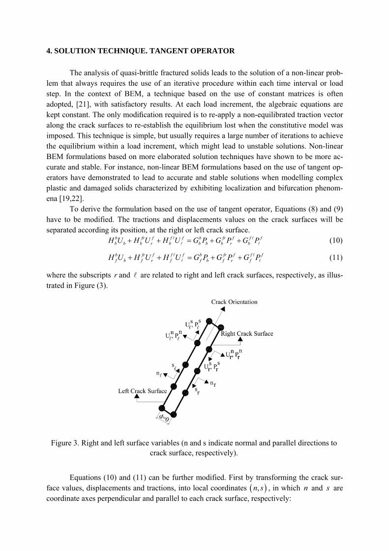
To derive the formulation based on the use of tangent operator, Equations (8) and (9) have to be modified. The tractions and displacements values on the crack surfaces will be separated according its position, at the right or left crack surface.

b fr f f f b fr f f fb b b r b b b b r bH U H U H U G P G P G P

(10)

b fr f f f b fr f f ff b f r f f b f r fH U H U H U G P G P G P

(11)

where the subscripts r and are related to right and left crack surfaces, respectively, as illus-trated in Figure (3).

Figure 3. Right and left surface variables (n and s indicate normal and parallel directions to crack surface, respectively).

Equations (10) and (11) can be further modified. First by transforming the crack sur-face values, displacements and tractions, into local coordinates ,n s , in which n and s are coordinate axes perpendicular and parallel to each crack surface, respectively:

 

b frs f frn f f s f f n f b frs f frn f f s f f n fb b b rs b rn b s b n b b b rs b rn b s b nH U H U H U H U H U G P G P G P G P G P

(12)

b frs f frn f f s f f n f b frs f frn f f s f f n ff b f rs f rn f s f n f b f rs f rn f s f nH U H U H U H U H U G P G P G P G P G P

(13)

After these modifications, the relative displacements on the crack surfaces can be in-cluded in the formulation. The crack relative displacements on directions parallel and perpen-dicular to crack surfaces, su and nu respectively, are used to replace the displacement compo-nents along the left crack side.

f f f fs s rs s s rsu U U U u U (14)

f f f fn n rn n n rnu U U U u U (15)

After these modifications, Equations (12) and (13) can be rewritten as follow:

b frs f s f frn f n f f s f nb b b b rs b b rn b s b nH U H H U H H U H u H u

b frs f frn f f s f f n fb b b rs b rn b s b nG P G P G P G P G P

(16)

b frs f s f frn f n f f s f nf b f f rs f f rn f s f nH U H H U H H U H u H u

b frs f frn f f s f f n ff b f rs f rn f s f nG P G P G P G P G P

(17)

Equations (16) and (17) represent the equilibrium of solid containing cracks. For the case of non-linear fracture problems, these two last equations have to be written and solved within the context of incremental problems. Thus, Equations (16) and (17) have to be conven-iently rewritten in its incremental forms. Firstly, these equations have to be written in rates and then transformed into their incremental forms by performing the relevant time integrals over a typical time increment 1n nt t t . For the postulated problem, the corresponding incremental forms of Equations (16) and (17) is simple and obtained by replacing all bound-ary and crack values x by their increments x .

For a given load increment, Equations (16) and (17) can be further modified by apply-ing the known boundary conditions. As usual in BEM formulations, all unknown boundary values are stored in a vector x and cumulate the known boundary values effects into inde-pendent vectors bf and ff . After these modifications, the functions below can be written, to express the equilibrium of solid containing cracks:

frs f s f frn f n f f s f nb b b b rs b b rn b s b nY a x H H U H H U H u H u

frs f s f frn f s fb b b s b b nf G G f G G f (18)

frs f s f frn f n f f s f nf f f f rs f f rn f s f nY a x H H U H H U H u H u

frs f s f frn f s ff f f s f f nf G G f G G f (19)

In Equations (18) and (19), the matrices ba and fa contain the coefficients of matrices referred to unknown boundary displacements and tractions. These two last equations can be further modified to emphasize the variables related to cohesive criterion in the non-linear process. These variables are the crack relative displacement and the traction, both in n direc-tion. Then, the two last equations above can be rewritten as:

f n frn f n fb b b n b b b nY A X H u F G G f (20)

f n frn f n ff f f n f f f nY A X H u F G G f (21)

In these equations, the matrices bA and fA contain the coefficients of matrices referred to unknown boundary and right crack displacements increments ( , f

b rsU U and frnU ),

boundary tractions ( bP ) and the crack relative displacement at the s direction ( su ). The known boundary and crack values, this last one only at the s direction, are taken into account with independent vectors bF and fF . Along the crack surfaces, only the traction compo-nents in n direction are considered in the non-linear process. The traction components in di-rection s are neglected according to the cohesive crack model.

The non-linear system of equations given in (20) and (21) can be solved by applying Newton–Raphson’s scheme, for which an iterative process may be required to achieve the equilibrium. By linearizing Equations (20) and (21) and using only the first term of Taylor’s expansion one has:

, ,... , ,...0

i i i ib k nk b k nki i i

b nk k nki ik nk

Y X u Y X uY u X u

X u

(22)

, ,... , ,...0

i i i if k nk f k nki i i

f nk k nki ik nk

Y X u Y X uY u X u

X u

(23)

The derivative terms in Equations (22) and (23) give the global tangent operator [C]. Thus, carrying out all indicated derivates in these two last equations, the tangent operator for the case of cohesive crack can be obtained. Therefore:

f n frn f n fb b b b n n

f n frn f n ff f f f n n

A H G G f uC

A H G G f u

(24)

where the derivate fn nf u is obtained by differentiating properly the cohesive crack laws

presented in section 2. Thus, the corrections ikX and i

nku are obtained by solving the lin-earized system represented by equations (22) and (23):

1

iib nkk

i ink f nk

Y uXC

u Y u

(25)

Within a given load increment k the solution is obtained by cumulating the corrections calculated using Equation (25):

1i i ik k kX X X (26)

1i i ink nk nku u u (27)

After solving the implicit non-linear system of equations using tangent operator in terms of kX and nku all variables have to be updated before applying the next load incre-ment. The tolerance to stop the iterative process within an increment of load is applied on the variation of the crack opening displacement corrections, i.e, 1i iu u tolerance .

5. CRACK GROWTH SCHEME

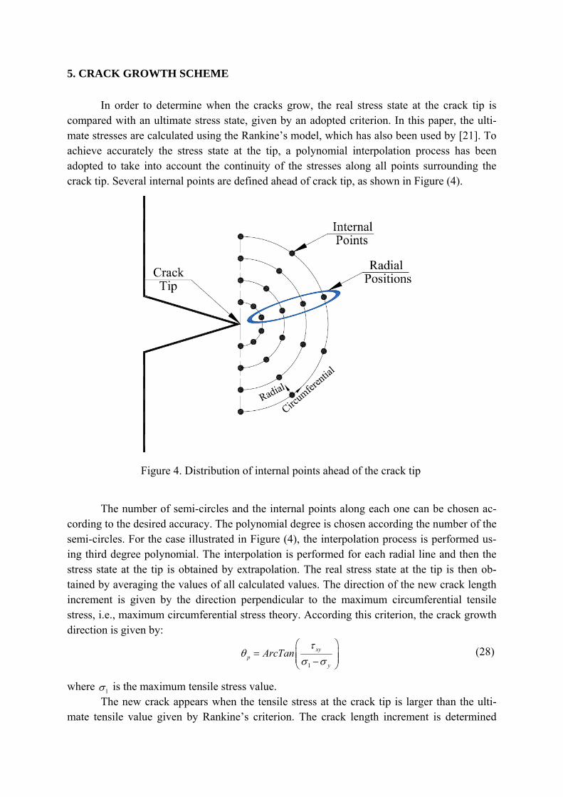
In order to determine when the cracks grow, the real stress state at the crack tip is compared with an ultimate stress state, given by an adopted criterion. In this paper, the ulti-mate stresses are calculated using the Rankine’s model, which has also been used by [21]. To achieve accurately the stress state at the tip, a polynomial interpolation process has been adopted to take into account the continuity of the stresses along all points surrounding the crack tip. Several internal points are defined ahead of crack tip, as shown in Figure (4).

Figure 4. Distribution of internal points ahead of the crack tip

The number of semi-circles and the internal points along each one can be chosen ac-cording to the desired accuracy. The polynomial degree is chosen according the number of the semi-circles. For the case illustrated in Figure (4), the interpolation process is performed us-ing third degree polynomial. The interpolation is performed for each radial line and then the stress state at the tip is obtained by extrapolation. The real stress state at the tip is then ob-tained by averaging the values of all calculated values. The direction of the new crack length increment is given by the direction perpendicular to the maximum circumferential tensile stress, i.e., maximum circumferential stress theory. According this criterion, the crack growth direction is given by:

1

xyp

y

ArcTan

(28)

where 1 is the maximum tensile stress value. The new crack appears when the tensile stress at the crack tip is larger than the ulti-

mate tensile value given by Rankine’s criterion. The crack length increment is determined

adjusting the size of the element in such a way that the stress state at the new crack tip, calcu-lated by the maximum tensile stress criterion, is equal to the ultimate tensile.

6. APPLICATIONS

Three examples were chosen to illustrate the efficiency and robustness of the proposed BEM formulation in modelling non-linear cohesive crack propagation analysis. The first ex-ample presents the analysis of crack growth in a three point bending concrete beam. A four point bending concrete structure is analyzed in the second application, while a four point bending multi-fractured concrete structure is considered as last application.

6.1. Concrete three point bending beam

The structure considered in this example is illustrated in Figure (5). It is a three point bending concrete structure which has 800 mm of length, 200 mm of height and contains a central notch of 50 mm. The experimental results of this example are given by [21], from which the following material parameters were chosen: ultimate tensile stress 3.0c

tf MPa ; Young's modulus E=30,000 MPa; Poisson's ν=0.15; and fracture energy Gf=75 N/m.

Figure 5. Three point bending beam

The analysis of this example was performed considering the three cohesive laws dis-

cussed earlier (linear, bi-linear and exponential). The load has been applied in 25 load incre-ments and the convergence has been verified with a tolerance of 10−5.

Figure (6) shows the comparative among experimental result obtained by [21] and numerical responses achieved by the BEM formulations described earlier. In this figure, the suffix CTO identifies the results obtained using tangent operator. According the results shown in Figure (6) good agreement is observed among the experimental and numerical re-sults. Figure (7) describes the crack growth path observed in this analysis.

The number of iterations required by each model and cohesive crack law to achieve the convergence is illustrated in Figure (8). According this figure, the formulation based on tangent operator has demonstrated be faster than the classical procedure (constant operator).

The tangent operator formulation is faster even in the beginning of the analysis, when the non-linear cohesive crack length is small. This behaviour occurs because the tangent operator is constant when linear and bi-linear cohesive laws are adopted. Then, the non-linear process may achieve the convergence using only one iteration. This situation is observed when no changes occur in the cohesive zone, i.e, none node leaves the cohesive zone from one iteration to the next.

Figure 6. Load × displacement curves.

Figure 7. Crack growth path. Initial notch and final crack path.

Figure 8. Number of iterations required to reach the convergence.

6.2. Concrete three point bending beam

The four point beam considered in this example is shown in Figure (9). The geometry is given by its length of 675mm, height of 150mm and central notch 75mm deep. The material properties were taken from [23], who have performed a laboratory test: tensile strength

3.0ctf MPa , Young’s modulus 37.000E MPa , Poisson’s ratio 0.20 and fracture energy

69fG N m .

Figure 9. Four point bending beam. Dimensions in mm.

For the present analysis three cohesive laws were used: linear, bi-linear and exponen-tial. The load was applied for all cases in 24 increments and the adopted tolerance within each increment was 510 . The two non-linear system solution techniques discussed previously were tested: (a) using constant operator (b) using tangent operator. The results obtained are given in

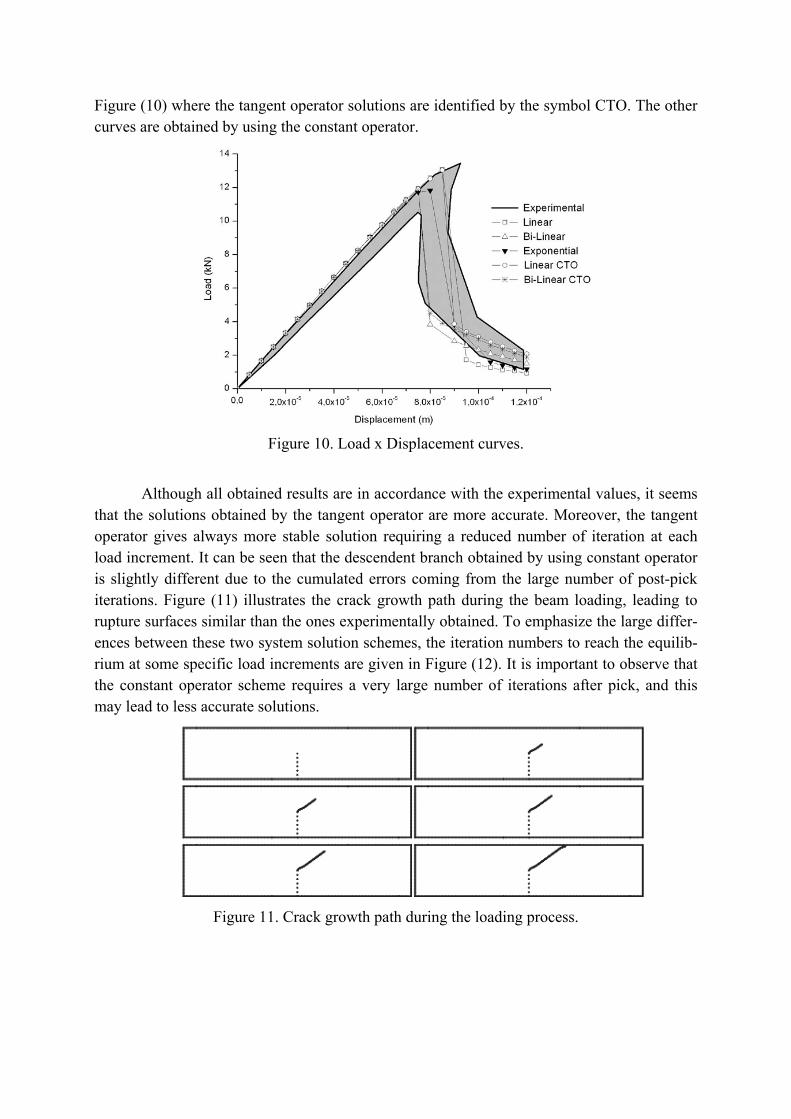
Figure (10) where the tangent operator solutions are identified by the symbol CTO. The other curves are obtained by using the constant operator.

Figure 10. Load x Displacement curves.

Although all obtained results are in accordance with the experimental values, it seems that the solutions obtained by the tangent operator are more accurate. Moreover, the tangent operator gives always more stable solution requiring a reduced number of iteration at each load increment. It can be seen that the descendent branch obtained by using constant operator is slightly different due to the cumulated errors coming from the large number of post-pick iterations. Figure (11) illustrates the crack growth path during the beam loading, leading to rupture surfaces similar than the ones experimentally obtained. To emphasize the large differ-ences between these two system solution schemes, the iteration numbers to reach the equilib-rium at some specific load increments are given in Figure (12). It is important to observe that the constant operator scheme requires a very large number of iterations after pick, and this may lead to less accurate solutions.

Figure 11. Crack growth path during the loading process.

Figure 12. Required number of iterations for the tested solution techniques.

6.3. Multi-fractured concrete structure

In this application, the structure presented in Figure (13) is analyzed. This is a concrete beam subjected to a four bending test. This structure has 1.5 m of length and 0.50 m of high as shown in the same figure. The material properties adopted for this application were: tensile strength 3.0c

tf MPa , Young’s modulus 30,000E MPa , Poisson’s ratio 0.20 and fracture energy 75fG N m .

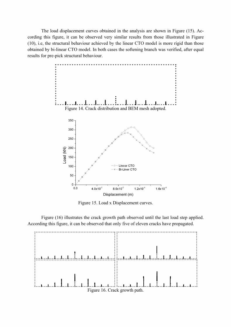
In this analysis, eleven cracks were distributed along the lower structural boundary as illustrated in Figure (14). In the same figure is also presented the BEM mesh considered for this analysis. Therefore, the performance of the proposed non-linear formulation in the case of multiple cracks is evaluated. Only two cohesive crack laws were considered in this example: linear and bi-linear. Both cohesive laws were coupled with tangent operator formulation. The load was applied in 25 increments and the adopted tolerance within each increment was 510 .

Figure 13. Dimensions and boundary conditions for the structure.

1,5 m

0,5

m

F/2 F/2

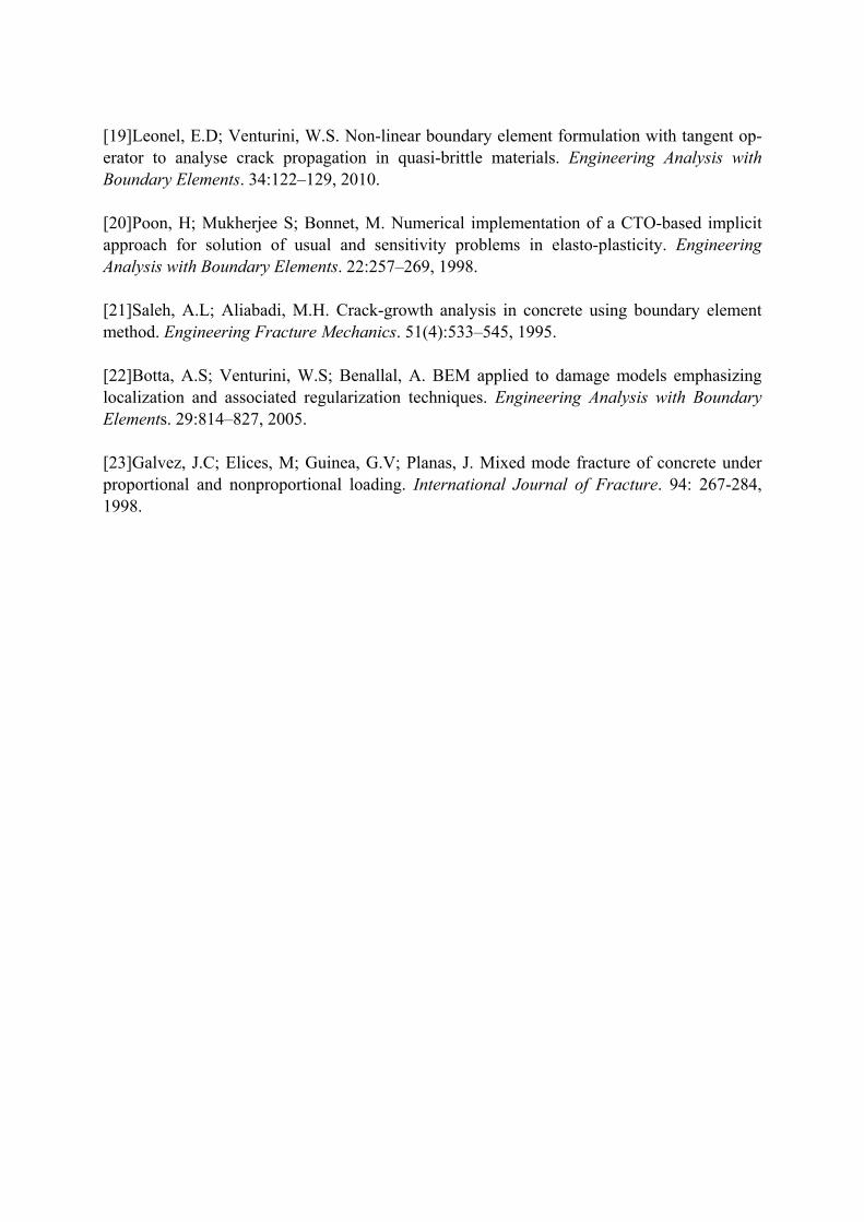
The load displacement curves obtained in the analysis are shown in Figure (15). Ac-cording this figure, it can be observed very similar results from those illustrated in Figure (10), i.e, the structural behaviour achieved by the linear CTO model is more rigid than those obtained by bi-linear CTO model. In both cases the softening branch was verified, after equal results for pre-pick structural behaviour.

Figure 14. Crack distribution and BEM mesh adopted.

Figure 15. Load x Displacement curves.

Figure (16) illustrates the crack growth path observed until the last load step applied. According this figure, it can be observed that only five of eleven cracks have propagated.

Figure 16. Crack growth path.

7. CONCLUSION

In this paper, crack propagation process in quasi-brittle materials has been studied. The complex structural behaviour arising from these materials can be modelled by solving a non-linear system of equations which appears due the dependency between crack opening displacement and tractions along the normal direction to the crack lips. To simulate this non-linear structural problem, BEM has shown to be an accurate and efficient alternative. Two non-linear BEM formulations have been developed and implemented in this paper. The first applies a constant operator, where the non-linear problem is solved by keeping constant all relevant matrices and calculating, at each load step, the non-equilibrated vector force. The second approach is developed by using a tangent operator. In this case, the derivative set of the non-linear equations is used and the problem is faster solved. In this case the problem is solved implicitly using the tangent operator expression. The formulation based on the tangent operator has shown to be more stable and lead to more accurate results in comparison with the classical procedure (constant operator). The use of tangent operator has shown to be always recommended to analyze crack propagation problems, particularly for the cases where the after pick region is reached.

This kind of formulation may be applied in other non-linear problems in the future. Contact problems and crack growth in reinforced structures, for instance, can be modelled using this efficient approach.

Acknowledgements

Sponsorship of this research project by the São Paulo State Foundation for Research – FAPESP - is greatly appreciated.

8. REFERENCES

[1] Barenblatt, G.I. The mathematical theory of equilibrium cracks in brittle fracture. Ad-vances in Applied Mechanics. 7:55–129, 1962. [2]Carpinteri, A. Post-peak and post-bifurcation analysis of cohesive crack propagation. En-gineering Fracture Mechanics. 32:265–278, 1989. [3]Dugdale, D.S. Yelding of steel sheets containing slits. Journal of Mechanics and Physics of Solids. 8:100–104, 1960. [4] Hillerborg, A; Modeer, M; Peterson, P.E. Analysis of crack formation and crack growth in concrete by mean of failure mechanics and finite elements. Cement Concrete Research. 6:773–782, 1976.

[5] Bouchard, P.O; Bay, F; Chastel, Y. Numerical modelling of crack propagation: automatic remeshing and comparison of different criteria. Computer Methods in Applied Mechanics and Engineering. 192:3887–3908, 2002. [6] Patzak, B; Jirasek, M. Adaptive resolution of localized damage in quasi-brittle materials. Journal of Engineering Mechanics. 130:720–732, 2004. [7] Moes, N; Dolbow, J; Belytschko, T. A finite element method for crack growth without remeshing, Int J Numer Meth Eng. 46, pp. 131–150, 1999. [8] Belytschko, T; Liu, Y.Y. Element free Galerkin methods. Int J Numer Meth Eng. 37, pp. 229–256, 1994. [9]Cruse, T.A. Boundary Element Analysis in computational fracture mechanics. Dordrecht: Kluwer Academic Publishers; 1988. [10]Crouch, S. L. Solution of plane elasticity problems by the displacement discontinuity method. International Journal of Numerical Methods in Engineering. 10:301-343, 1976. [11]Portela, A; Aliabadi, M.H; Rooke, D.P. Dual Boundary element method: efficient imple-mentation for crack problems. International Journal of Numerical Methods in Engineering. 33:1269-1287, 1992. [12]Yan, X. Microdefect interacting with a finite main crack. Journal of Strain Analysis Engi-neering Design. 40:421–430, 2005. [13]Kebir, H; Roelandt, J.M; Chambon, L. Dual boundary element method modelling of air-craft structural joints with multiple site damage. Engineering Fracture Mechanics. 73:418-434, 2006. [14]Leonel, E.D; Venturini, W.S. Dual boundary element formulation applied to analysis of multi-fractured domains. Engineering Analysis with Boundary Elements. 34: 1092-1099, 2010. [15] Leonel, E.D; Venturini, W.S. Multiple random crack propagation using a boundary ele-ment formulation, Engineering Fracture Mechanics, 78, 1077–1090, 2011. [16] Leonel, E.D; Beck, A.T; Venturini, W.S. On the performance of response surface and direct coupling approaches in solution of random crack propagation problems. Structural Safety. 33 (4-5), pp. 261-274, 2011. [17 ] Leonel, E.D; Venturini, W.S; Chateauneuf, A. A BEM model applied to failure analysis of multi-fractured structures. Engineering Failure Analysis, 18, (6) 1538-1549, 2011. [18 ]Kumar, V; Mukherjee, S. Boundary-integral equation formulation for time-dependent inelastic deformation in metals. International Journal of Mechanical Sciences. 19(12):713–724, 1977.

[19]Leonel, E.D; Venturini, W.S. Non-linear boundary element formulation with tangent op-erator to analyse crack propagation in quasi-brittle materials. Engineering Analysis with Boundary Elements. 34:122–129, 2010. [20]Poon, H; Mukherjee S; Bonnet, M. Numerical implementation of a CTO-based implicit approach for solution of usual and sensitivity problems in elasto-plasticity. Engineering Analysis with Boundary Elements. 22:257–269, 1998. [21]Saleh, A.L; Aliabadi, M.H. Crack-growth analysis in concrete using boundary element method. Engineering Fracture Mechanics. 51(4):533–545, 1995. [22]Botta, A.S; Venturini, W.S; Benallal, A. BEM applied to damage models emphasizing localization and associated regularization techniques. Engineering Analysis with Boundary Elements. 29:814–827, 2005. [23]Galvez, J.C; Elices, M; Guinea, G.V; Planas, J. Mixed mode fracture of concrete under proportional and nonproportional loading. International Journal of Fracture. 94: 267-284, 1998.