NON-LINEAR REGRESSION MODELS - VirtualPanicvirtualpanic.com/anonymousftplistings/ebooks/ECONOMICS/Amemiya...Single equation-i.i.d. case 2.1. Model ... Non -linear Regression Models

Chapter 6

NON-LINEAR REGRESSION MODELS

TAKESHI AMEMIYA*

Stanford University

Contents

1. Introduction 334 2. Single equation-i.i.d. case 336

2.1. Model 336 2.2. Asymptotic properties 337 2.3. Computation 341 2.4. Tests of hypotheses 347 2.5. Confidence regions 352

3. Single equation-non-i.i.d. case 354 3. I. Autocorrelated errors 354 3.2. Heteroscedastic errors 358

4. Multivariate models 359 5. Simultaneous equations models 362

5.1. Non-linear two-stage least squares estimator 362 5.2. Other single equation estimators 370 5.3. Non-linear simultaneous equations 375 5.4. Non-linear three-stage least squares estimator 376 5.5. Non-linear full information maximum likelihood estimator 379

References 385

*This work was supported by National Science Foundation Grant SE%7912965 at the Institute for Mathematical Studies in the Social Sciences, Stanford University. The author is indebted to the following people for valuable comments: R. C. Fair, A. R. Gallant, Z. Griliches, M. D. Intriligator, T. E. MaCurdy, J. L. Powell, R. E. Quandt, N. E. Savin, and H. White.

Handbook of Econometrics, Volume I, Edited by Z. Griliches and M.D. Intriligator 0 North-Holland Publishing Company, 1983

334 T. Amemiya

1. Introduction

This is a survey of non-linear regression models, with an emphasis on the theory of estimation and hypothesis testing rather than computation and applications, although there will be some discussion of the last two topics. For a general discussion of computation the reader is referred to Chapter 12 of this Handbook by Quandt. My aim is to present the gist of major results; therefore, I will sometimes omit proofs and less significant assumptions. For those, the reader must consult the original sources.

The advent of advanced computer technology has made it possible for the econometrician to estimate an increasing number of non-linear regression models in recent years. Non-linearity arises in many diverse ways in econometric applications. Perhaps the simplest and best known case of non-linearity in econometrics is that which arises as the observed variables in a linear regression model are transformed to take account of the first-order autoregression of the error terms. Another well-known case is the distributed-lag model in which the coefficients on the lagged exogenous variables are specified to decrease with lags in a certain non-linear fashion, such as geometrically declining coefficients. In both of these cases, non-linearity appears only in parameters but not in variables.

More general non-linear models are used in the estimation of production functions and demand functions. Even a simple Cobb-Douglas production function cannot be transformed into linearity if the error term is added rather than multiplied [see Bodkin and Klein (1967)]. CES [Arrow, Chenery, Minhas and Solow (196 l)] and VES [Revankar (1971)] production functions are more highly non-linear. In the estimation of expenditure functions, a number of highly non-linear functions have been proposed (some of these are used in the supply side as well)-Translog [Christensen, Jorgenson and Lau (1975)], Generalized Leontief [Diewert (1974)], S-Branch [Brown and Heien (1972)], and Quadratic [Howe, Pollack and Wales (1979)], to name a few. Some of these and other papers with applications will be mentioned in various relevant parts of this chapter.

The non-linear regression models I will consider in this chapter can be written in their most general form as

(1.1)

where y,, .x,, and (Y~ are vectors of endogenous variables, exogenous variables, and parameters, respectively, and uif are unobservable error terms with zero mean. Eqs. (1. l), with all generality, constitute the non-linear simultaneous equations model, which is analyzed in Section 5. I devote most of the discussion in the chapter to this section because this area has been only recently developed and therefore there is little account of it in general references.

Ch. 6: Non -linear Regression Models 335

Many simpler models arising as special cases of (1.1) are considered in other sections. In Section 2 I take up the simplest of these, which I will call the standard non-linear regression model, defined by

Y,=f(x,&+% t=1,2 ,..., T, 0.2)

where (u,} are scalar i.i.d. (independent and identically distributed) random variables with zero mean and constant variance. Since this is the model which has been most extensively analyzed in the literature, I will also devote a lot of space to the analysis of this model. Section 3 considers the non-i.i.d. case of the above model, and Section 4 treats its multivariate generalization.

Now, I should mention what will not be discussed. I will not discuss the maximum likelihood estimation of non-linear models unless the model is written in the regression form (1.1). Many non-linear models are discussed elsewhere in this Handbook; see, for example, the chapters by Dhrymes, McFadden, and Maddala. The reader is advised to recognize a close connection between the non-linear least squares estimator analyzed in this chapter and the maximum likelihood estimator studied in the other chapters; essentially the same techniques are used to derive the asymptotic properties of the two estimators and analogous computer algorithms can be used to compute both.

I will not discuss splines and other methods of function approximation, since space is limited and these techniques have not been as frequently used in econometrics as they have in engineering applications. A good introduction to the econometric applications of spline functions can be found in Poirier (1976).

Above I mentioned the linear model with the transformation to reduce the autocorrelation of the error terms and the distributed-lag model. I will not specifically study these models because they are very large topics by themselves and are best dealt with separately. (See the chapter by Hendry, Pagan, and Sargan in this Handbook). There are a few other important topics which, although non-linearity is involved, woud best be studied within another context, e.g. non-linear error-in-variable models and non-linear time-series models. Regarding these two topics, I recommend Wolter and Fuller (1978) and Priestley (1978). Finally, I conclude this introduction by citing general references on non-linear regression models. Malinvaud (1970b) devotes one long chapter to non-linear regression models in which he discusses the asymptotic properties of the non- linear least squares estimator in a multivariate model. There are three references which are especially good in the discussion of computation algorithms, confidence regions, and worked out examples: Draper and Smith (1966) Bard (1974) and Judge, Griffiths, Hill and Lee (1980). Several chapters in Goldfeld and Quandt (1972) are devoted to the discussion of non-linear regression models. Their Chapter 1 presents an excellent review of optimization techniques which can be used in the computation of both the non-linear least squares and the maximum likelihood estimators. Chapter 2 discusses the construction of confidence regions

336 T. Amemiya

in the non-linear regression model and the asymptotic properties of the maximum likelihood estimator (but not of the non-linear least squares estimator). Chapter 5 considers the Cobb-Douglas production function with both multiplicative and additive errors, and Chapter 8 considers non-linear (only in variables) simultaneous equations models. There are two noteworthy survey articles: Gallant (1975a), with emphasis on testing and computation, and Bunke, Henscheke, Strtiby and Wisotzki (1977), which is more theoretically oriented. None of the above-mentioned references, however, discusses the estimation of simultaneous equations models non-linear both in variables and parameters.

2. Single equation-i.i.d. case

2.1. Model

In this section I consider the standard non-linear regression model

Y,=fb,Jo)+%~ t=1,2 ,..., T, (2.1) where y, is a scalar endogenous variable, x, is a vector of exogenous variables, & is a K-vector of unknown parameters, and {u,} are unobservable scalar i.i.d. random variables with Eu, = 0 and Vu, = ut, another unknown parameter. Note that, unlike the linear model wheref(x,, &) = x&, the dimensions of the vectors x, and &-, are not necessarily the same. We will assume that f is twice continuously differentiable. As for the other assumptions on f, I will mention them as they are required for obtaining various results in the course of the subsequent discussion.

Econometric examples of (2.1) include the Cobb-Douglas production function with an additive error,

Q, = p, Kf2L,B3 + u,,

and the CES (constant elasticity of substitution) production function:

(2.2)

(2.3)

Sometimes I will write (2.1) in vector notation as

Y =f(Po)+% (2.4)

where y, f( /3,-J, and u are T-vectors whose t th element is equal toy,, f( x,, &), and u,, respectively. I will also use the symbolf,(&) to denote f(x,, &,)_


The non-linear least squares (NLLS) estimator, denoted p, is defined as the value of /I that minimizes the sum of squared residuals

S,(P) = t [Yt -fhP)12. (2.5)

It is important to distinguish between the p that appears in (2.5), which is the argument of the function f(x,, m), and &, which is a fixed true value. In what follows, I will discuss the properties of p, the method of computation, and statistical inference based on 8.

2.2. Asymptotic properties

2.2.1. Consistency

The consistency of the NLLS estimator is rigorously proved in Jennrich (1969) and Malinvaud (1970a). The former proves strong consistency (j? converging to &, almost surely) and the latter weak consistency (p converging to &, in probability). Weak consistency is more common in the econometric literature and is often called by the simpler name of consistency. The main reason why strong consistency, rather than weak consistency, is proved is that the former implies the latter and is often easier to prove. I will mainly follow Jennrich’s proof but translate his result into weak consistency.

The consistency of b is proved by proving that plim T- ‘S,( j3) is minimized at the true value &. Strong consistency is proved by showing the same holds for the almost sure limit of T- ‘S,( /3) instead. This method of proof can be used to prove the consistency of any other type of estimator which is obtained by either minimizing or maximizing a random function over the parameter space. For example, I used the same method to prove the strong consistency of the maximum likelihood estimator (MLE) of the Tobit model in Amemiya (1973b).

This method of proof is intuitively appealing because it seems obvious that if T-l&( /3) is close to plim T-k&(/3) and if the latter is minimized at &,, then fi, which minimizes the former, should be close to &. However, we need the following three assumptions in order for the proof to work:

The parameter space B is compact (closed and bounded)

and & is its interior point. (2.6) S, ( @ ) is continuous in p . (2.7)

plim T- ‘S,(p) exists, is non-stochastic, and its convergence is uniform in p.

(2.8)

338 T. Amemiya

The meaning of (2.8) is as follows. Define S(p) = plim T- ‘S,( j3). Then, given E, S > 0, there exists To, independent of /I, such that for all T 2 To and for all P, PUT-‘&-(P)- S(P)1 ’ &I< 6.

It is easy to construct examples in which the violation of any single assumption above leads to the inconsistency of 8. [See Amemiya (1980).]

I will now give a sketch of the proof of the consistency and indicate what additional assumptions are needed as I go along. From (2.1) and (2.5), we get

=A,+A,+A,, (2.9) where c means CT=, unless otherwise noted. First, plim A, = ut by a law of large numbers [see, for example, Kolmogorov Theorem 2, p. 115, in Rao (1973)]. Secondly, for fixed &, and p, plim A, = 0 follows from the convergence of T-‘C[f,(&)- f,(p)]’ by Chebyshev’s inequality:

Since the uniform convergence of A, follows from the uniform convergence of the right-hand side of (2.10), it suffices to assume

converges uniformly in fi, , & E B. (2.11)

Having thus disposed of A, and A,, we need only to assume that lim A, is uniquely minimized at PO; namely,

lim+E[f,(&)-N)l’-o ifP*&. (2.12)

To sum up, the non-linear least squares estimator B of the model (2.1) is consistent if (2.6), (2.1 l), and (2112) are satisfied. I will comment on the significance and the plausibility of these three assumptions.

The assumption of a compact parameter space (2.6) is convenient but can be rather easily removed. The trick is to dispose of the region outside a certain compact subset of the parameter space by assuming that in that region T-‘~MPoF.MP)12 * IS sufficiently large. This is done by Malinvaud (1970a). An essentially similar argument appears also in Wald (1949) in the proof of the consistency of the maximum likelihood estimator.

It would be nice if assumption (2.11) could be paraphrased into separate assumptions on the functional form off and on the properties of the exogenous


sequence {x,}, which are easily verifiable. Several authors have attempted to obtain such assumptions. Jennrich (1969) observes that if f is bounded and continuous, (2.11) is implied by the assumption that the empirical distribution function of {x,} converges to a distribution function. He also notes that another way to satisfy (2.11) is to assume that {x,} are i.i.d. with a distribution function F, and f is bounded uniformly in p by a function which is square integrable with respect to F. Malinvaud (1970a) generalizes the first idea of Jennrich by introduc- ing the concept of weak convergence of measure, whereas Gallant (1977) generalizes the second idea of Jennrich by considering the notion of Cesaro summabil- ity. However, it seems to me that the best procedure is to leave (2.11) as it is and try to verify it directly.

The assumption (2.12) is comparable to the familiar assumption in the linear model that lim T- ‘X’X exists and is positive definite. It can be easily proved that in the linear model the above assumption is not necessary for the consistency of least squares and it is sufficient to assume (X’X)- ’ + 0. This observation suggests that assumption (2.12) can be relaxed in an analogous way. One such result can be found in Wu (198 1).

2.2.2. Asymptotic normality

The asymptotic normality of the NLLS estimator B is rigorously proved in Jennrich (1969). Again, I will give a sketch of the proof, explaining the required assumptions as I go along, rather than reproducing Jennrich’s result in a theorem-proof format.

The asymptotic normality of the NLLS estimator, as in the case of the MLE, can be derived from the following Taylor expansion:

(2.13)

where a2$/apap’ is a K x K matrix of second-order derivatives and p* lies between j? and &. To be able to write down (2.13), we must assume that f, is twice continuously differentiable with respect to p. Since the left-hand side of (2.13) is zero (because B minimizes S,), from (2.13) we obtain:

@(~_p,)=_ 1 a2sT [ Twl,.]‘$ %I,,- (2.14)

Thus, we are done if we can show that (i) the limit distribution of fi-‘(asT/a&&, is normal and (ii) T- ‘( 6’2ST/apap’)B* converges in probability to a non-singular matrix. We will consider these two statements in turn.

340 T. Amemiya

The proof of statement (i) is straightforward. Differentiating (2.5) with respect to @, we obtain:

Evaluating (2.15) at & and dividing it by @, we have:

1 as, -- = JT ap &l i

aft cu -I f ap Bo*

(2.15)

(2.16)

But it is easy to find the conditions for the asymptotic normality of (2.16) because the summand in the right-hand side is a weighted average of an i.i.d. sequence-the kind encountered in the least squares estimation of a linear model. Therefore, if we assume

exists and is non-singular,

then

1 as --t 0 afi PO

+ N(0,4&).

(2.17)

(2.18)

This result can be straightforwardly obtained from the Lindberg-Feller central limit theorem [Rao (1973, p. 128)] or, more directly, from of Anderson (197 1, Theorem 2.6.1, p. 23).

Proving (ii) poses a more difficult problem. Write an element of the matrix ~-l(a~s,/apap)~. ash@*). 0 ne might think that plim hT( /3*) = plim hT( &,) follows from the well-known theorem which says that the probability limit of a continuous function is the function of the probability limit, but the theorem does not apply because h, is in general a function of an increasing number of random variables y,, j2,. . . ,y,. But, by a slight modification of lemma 4, p. 1003, of Amemiya (1973b), we can show that if hr( p) converges almost surely to a certain non-stochastic function h( /?) uniformly in p, then plim hT( p*) = h(plim /I*) = h( &). Differentiating (2.15) again with respect to p and dividing by T yields

(2.19)

We must show that each of the three terms in the right-hand side of (2.19)


converges almost surely to a non-stochastic function uniformly in p. For this purpose the following assumptions will suffice:

converges uniformly in /I in an open neighborhood of /3,, ,

and (2.20)

converges uniformly in p in an open neighborhood of & .

(2.21)

Then, we obtain;

1 a$- PlimT apap, 8* =2C-

Finally, from (2.14), (2.18), and (2.22) we obtain:

(2.22)

(2.23)

The assumptions we needed in proving (2.23) were (2.17), (2.20), and (2.21) as well as the assumption that /? is consistent.

It is worth pointing out that in the process of proving (2.23) we have in effect shown that we have, asymptotically,

(2.24)

where I have put G = ( af/&3’),0, a F x K matrix. Note that (2.24) exactly holds in the linear case. The practical consequence of the approximation (2.24) is that all the results for the linear regression model are asymptotically valid for the non-linear regression model if we treat G as the regressor matrix. In particular, we can use the usual t and F statistics with an approximate precision, as I will explain more fully in Sections 2.4 and 2.5 below. Since the matrix G depends on the unknown parameters, we must in practice evaluate it at b.

2.3. Computation

Since there is in general no explicit formula for the NLLS estimator b, the minimization of (2.5) must usually be carried out by some iterative method. There

342 T. Amemiya

are two general types of iteration methods: general optimization methods applied to the non-linear least squares problem in particular, and procedures which are specifically designed to cope with the present problem. In this chapter I will discuss two representative methods - the Newton-Raphson iteration which belongs to the first type and the Gauss-Newton iteration which belongs to the second type - and a few major variants of each method. These cover a majority of the iterative methods currently used in econometric applications. Although not discussed here, I should mention another method sometimes used in econometric applications, namely the so-called conjugate gradient method of Powell (1964) which does not require the calculation of derivatives and is based on a different principle from the Newton methods. Much more detailed discussion of these and other methods can be found in Chapter 12 of this Handbook and in Goldfeld and Quandt (1972, ch. 1).

2.3.1. Newton - Raphson iteration

The Newton-Raphson method is based on the following quadratic approximation of a minimand (it also works for a maximand):

(2.25)

where B, is the initial estimate [obtained by a pure guess or by a method such as the one proposed by Hartley and Booker (1965) described below]. The second- round estimator & of the iteration is obtained by minimizing the right-hand side of (2.25). Therefore,

(2.26)

The iteration is to be repeated until the sequence {&} thus obtained converges to the desired degree of accuracy.

Inserting (2.26) into (2.25) and writing n + 1 and n for 2 and 1, we obtain:

(2.27)

The above equation shows two weaknesses of the Newton-Raphson iteration. (i) Even if (2.27) holds exactly, &(&+ ,) < S,(&) is not guaranteed unless (~2WWV’)~” is a positive definite matrix. (ii) Even if the matrix is positive


definite, &, + , - fi,, may be too large or too small- if it is too large, it overshoots the target, and if it is too small, the speed of convergence is slow.

The first weakness may be alleviated if we modify (2.26) as

(2.28)

where I is the identity matrix and (Y, is a scalar to be appropriately chosen by the researcher subject to the condition that ( a2&/apap’)jn + a,Z is positive definite. This modification was proposed by Goldfeld, Quandt and Trotter (1966) and is called quadratic hill-climbing (since they were considering maximization). See the same article or Goldfeld and Quandt (1972, ch. 1) for a discussion of how to choose (Y, and the convergence properties of the method.

The second weakness may be remedied by the modification:

(2.29)

where the scalar X, is to be appropriately determined. See Fletcher and Powell (1963) for a method to determine h, by a cubic interpolation of S,(p) along the current search direction. [This method is called the DFP iteration since Fletcher and Powell refined the method originally proposed by Davidon (1959).] Also, see Berndt, Hall, Hall and Hausman (1974) for another method to choose A,.

Ordinarily, the iteration (2.26) is to be repeated until convergence takes place. However, if B, is a consistent estimator of & such that @(b, - &,) has a proper limit distribution, the second-round estimator 8, has the same asymptotic distribution as B. In this case, a further iteration does not bring any improvement so far as the asymptotic distribution is concerned. This is shown below.

By a Taylor expansion of (a&/a/3);, around &, we obtain:

as, as, -I I ab j, = T Bo +

where p* lies between B,

(S, -PO)> (2.30) 8*

and &. Inserting (2.30) into (2.26) yields

dqP,-PO)= I- ( [ ~~,1’ gg~~*)m~l-~o)

(2.31)

344 T Amemiya

But, under the assumptions of Section 2.2 from which we proved the asymptotic normality of b, we have

Therefore,

(2.32)

(2.33)

where y means that both sides of the equation have the same non-degenerate limit distribution.

To start an iteration, we need an initial estimate. Since there may be more than one local minima in ST, it is helpful to use the starting value as close to the true value as possible. Thus, it would abe desirable to have available an easily computable good estimator, such as p,; all the better if it is consistent so that we can take advantage of the result of the preceding paragraph. Surprisingly, I know only one such estimator - the one proposed by Hartley and Booker (1965). Their initial estimator is obtained as follows. Let us assume for simplicity mK = T for some integer m and partition the set of integers (1,2,. . . , T) into K non-overlap- ping consecutive subsets !P,, !P2;, . . . , !PK, each of which contains m elements. If we define j$, =m-'ClsuyI and f&(/3)=m-LC,,yfi(/3), i=l,2,...,K, the Harley-Booker estimator is defined as the value of b that satisfies K equations:

Y(i)=(i)(P), i=1,2 K. ,**., (2.34)

Since (2.34) cannot generally be solved explicitly for p, one still needs an iteration to solve it. Hartley and Booker propose the minimization of EYE ,[ jjCi, - fCi,(p)12 by an iterative method, such as one of the methods being discussed in this section. This minimization is at least simpler than the original minimization of (2.5) because the knowledge that the minimand is zero at /3 = & is useful. However, if there are multiple solutions to (2.34), an iteration may lead to the wrong solution.

Hartley and Booker proved the consistency of their estimator. Jennrich (1969) gave a counterexample to their consistency proof; however, their proof can easily be modified to take account of Jennrich’s counter-example. A more serious weakness of the Hartley-Booker proof is that their assumptions are too restric- tive: one can easily construct a benign example for which their assumptions are violated and yet their estimator is consistent.


Gallant (1975a) suggested a simpler variation of the Hartley-Booker idea: just select K observations appropriately and solve them for p. This estimator is simpler to compute, but inconsistent. Nevertheless, one may obtain a good starting value by this method, as Gallant’s example shows.

2.3.2. Gauss-Newton iteration

This is the method specifically designed to calculate the NLLS estimator. Expand- ing f,(p) in a Taylor series around the initial estimate fi,, we get:

Substituting the right-hand side of (2.35) for f,(p) in (2.5) yields

(2.35)

(2.36)

The second-round estimator b2 of the Gauss-Newton iteration is obtained by minimizing the right-hand side of (2.36) with respect to p. Thus,

(2.37)

The iteration is to be repeated until convergence is obtained. By an argument similar to the one I used in proving (2.33), we can prove that the asymptotic distribution of 8, defined in (2.37) is the same as that of B if we use a consistent estimator (such as the Hartley-Booker estimator) to start this iteration. An advantage of the Gauss-Newton iteration over the Newton-Raphson iteration is that the former requires only the first derivatives off,.

The Gauss-Newton iteration may be alternatively motivated as follows. Evaluating the approximation (2.35) at &, and inserting it into eq. (2.1) yields

(2.38)

Then, the second-round estimator b2 can be obtained as the least squares estimator of /3,, applied to the linear regression equation (2.38), where the whole left-hand side is treated as the dependent variable and (af,/J/3’);, as the vector of independent variables. Eq. (2.38) reminds us of the point raised above: namely, the non-linear regression model asymptotically behaves like the linear regression model if we treat (af/&‘fi’)j as the regressor matrix.

346 T A men1iya

The Gauss-Newton iteration suffers from weaknesses similar to those of the Newton-Raphson iteration: namely, the possibility of a total or near singularity of the matrix to be inverted in (2.37), and the possibility of too much or too little change from /$, to &,+ ,.

In order to deal with the first weakness, Marquardt (1963) proposed a modification:

where (Y, is a positive scalar to be appropriately determined by a rule based on the past behavior of the algorithm.

In order to deal with the second weakness, Hartley (1961) proposed the following modification. First, calculate

(2.40)

and, secondly, choose A, so as to minimize

$4 ii + %A,)~ O_Ih,_Il. (2.41)

Hartley proves that under general conditions his iteration converges to a stationary point: that is, a root of the normal equation &S,/ap = 0. He also proves (not so surprisingly) that if the iteration is started at a point sufficiently close to b, it converges to b. See Tomheim (1963) for an alternative proof of the convergence of the Hartley iteration. Some useful comments on Marquardt’s and Hartley’s algorithms can be found in Gallant (1975a). The methods of determin- ing A, in the Newton-Raphson iteration (2.29) mentioned above can be also applied to the determination of A,, in (2.41).

Jennrich (1969) proves that if the Gauss-Newton iteration is started at a point sufficiently close to the true value &, and if the sample size T is sufficiently large, the iteration converges to &,. This is called the asymptotic stability of the iteration. The following is a brief sketch of Jenmich’s proof. Rewrite the Gauss- Newton iteration (2.37) as (I have also changed 1 to n and 2 to n + 1 in the subscript)

b”+,=h(s,>? (2.42)

where h is a vector-valued function implicitly defined by (2.37). By a Taylor


expansion:

(2.43)

where /3:_ , lies between &, and &_ , . If we define A,, = (ah /a/3’),, and denote the largest characteristic root of AkA, by h,, we can show that A, + 0 almost surely for all n as T + 00 and hence

h, + 0 almost surely for all n as T + CO. (2.W

But (2.44) implies two facts. First, the iteration converges to a stationary point, and secondly, this stationary point must lie sufficiently close to the starting value 8, since

(,i~-p,)l(~~--,)~S’6(1+h,+hlXz+ *-. +h,X,.+_*), (2.45)

where 6 = & - 8,. Therefore, this stationary point must be B if 8, is within a neighborhood of & and if b is the unique stationary point in the same neighborhood.

In closing this section I will mention several empirical papers in which the above-mentioned and related iterative methods are used. Bodkin and Klein (1967) estimated the Cobb-Douglas (2.2) and the CES (2.3) production functions by the Newton-Raphson method. Charatsis (1971) estimated the CES production function by a modification of the Gauss-Newton method similar to that of Hartley (1961) and showed that in 64 samples out of 74, it converged in six iterations. Mizon (1977), in a paper the major aim of which was to choose among nine production functions, including the Cobb-Douglas and CES, used the conjugate gradient method of Powell (1964). Miion’s article is a useful compendium on the econometric application of various statistical techniques such as sequential testing, Cox’s test of separate families of hypotheses [Cox (1961, 1962)], the Akaike Information Criterion [Akaike (1973)], the Box-Cox transformation [Box and Cox (1964)], and comparison of the likelihood ratio, Wald, and Lagrange multiplier tests (see the end of Section 2.4 below). Sargent (1978) estimates a rational expectations model (which gives rise to non-linear constraints among parameters) by the DFP algorithm mentioned above.

2.4. Tests of hypotheses

In this section I consider tests of hypotheses on the regression parameters p. It is useful to classify situations into four cases depending on the nature of the

348 T. Amemiya

Table 2.1 Four cases of hypotheses tests -

Non-normal

Linear I II Non-linear III IV

hypotheses and the distribution of the error term as depicted in Table 2.1. I will discuss the t and F tests in Case I and the likelihood ratio, Wald, and Rao tests in Case IV. I will not discuss Cases II and III because the results in Case IV are a fortiori valid in Cases II and III.

2.4.1. Linear hypotheses under normality

Partition the parameter vector as fi’ = (&,,, &), where &,, is a K,-vector and &) is a K,-vector. By a linear hypothesis I mean a hypothesis which specifies that &) is equal to a certain known value PC*). Student’s t test is applicable if K, = 1 and theFtestifK,>l.

The hypothesis of the form Q/3 = c, where Q is a known K, X K matrix and c is a known K,-vector, can be transformed into a hypothesis of the form described above and therefore need not be separately considered. Assuming Q is full rank, we can find a K, X K matrix R such that (R’, Q’) = A’ is non-singular. If we define (Y = A/3 and partition (Y’ = (‘Y;,), (Y{*)), the hypothesis Q/3 = c is equivalent to the hypothesis a(Z) = c.

As noted after eq. (2.24), all the results of the linear regression model can be extended to the non-linear model .by treating G = ( af/&3’),0 as the regressor matrix if the assumptions of Section 2.2 are satisfied. Since &, is unknown, we must use G = (af/ap)j in practice. We will generalize the t and F statistics of the linear model by this principle. If K, = 1, we have approximately

-qK($z,-%J _ t(T_ K)

gm ’ (2.46)

where L! is the last diagonal element (if &) is the i th element of p, the i th diagonal element) of (&G)-’ and t(T- K) denotes Student’s t distribution with T - K degrees of freedom. For the case K, 2 1, we have asymptotically under the null hypothesis:


where J’= (0, I), 0 being the K, X K, matrix of zeros and I being the identity matrix of size K,, and F( K,, T - K) denotes the F distribution with K, and T - K degrees of freedom.

Gallant (1975a) examined the accuracy of the approximation (2.46) by a Monte Carlo experiment using the model

f(x,, P) = PA + P2x2t + P4eS+3r. (2.48)

For each of the four parameters, the empirical distribution of the left-hand side of (2.46) matched the distribution of t(T - K) reasonably well, although, as we would suspect, the performance was the poorest for 8,.

In testing & = p(Z) when K, 2 1, we may alternatively use the asymptotic approximation (under the null hypothesis):

(T-K)[%(i+&@)l _ J-(K

K2wv 29 T_ K) (2.49)

where b is the constrained non-linear least squares estimator obtained by minimizing S,( /3) subject to pc2, = pc2). Although, as is well known, the statistics (2.47) and (2.49) are identical in the linear model, they are different in the non-linear model.

The study of Gallant (1975~) sheds some light on the choice between (2.47) and (2.49). He obtained the asymptotic distribution of the statistics (2.47) and (2.49) under the alternative hypothesis as follows. Regarding S,(b), which appears in both formulae, we have asymptotically:

S,(B) = u’[l-G(G’G)-‘G’]u, (2.50)

where G = ( af/a/3’)s, as before. Define G, = ( af/a&,),, Then, Gallant shows (asymptotically) that

s,(p) = (u+ a)![~- G,(G;GJ’G;](~ + a), (2.51)

- where 6 = f(P&- f(P;T,, /$) Ilf(PckN3~,,~ 42))l12. wll

in which /?& is the value of &, that minimizes = x’x for any vector x.) He also shows

(2.52)

350 T. Amemiya

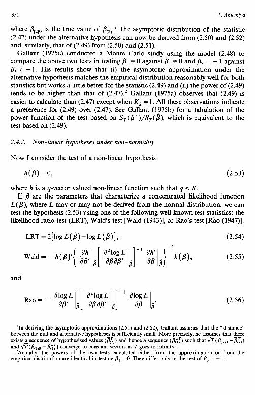
where fit2j0 is the true value of &.’ The asymptotic distribution of the statistic (2.47) under the alternative hypothesis can now be derived from (2.50) and (2.52) and, similarly, that of (2.49) from (2.50) and (2.5 1).

Gallant (1975~) conducted a Monte Carlo study using the model (2.48) to compare the above two tests in testing p, = 0 against p, t 0 and & = - 1 against & * - 1. His results show that (i) the asymptotic approximation under the alternative hypothesis matches the empirical distribution reasonably well for both statistics but works a little better for the statistic (2.49) and (ii) the power of (2.49) tends to be higher than that of (2.47).2 Gallant (1975a) observes that (2.49) is easier to calculate than (2.47) except when K, = 1. All these observations indicate a preference for (2.49) over (2.47). See Gallant (1975b) for a tabulation of the power function of the test based on S,(/?‘)/S,(&, which is equivalent to the test based on (2.49).

2.4.2. Non -linear hypotheses under non -normality

Now I consider the test of a non-linear hypothesis

h(P) = 0, (2.53)

where h is a q-vector valued non-linear function such that q < K. If /3 are the parameters that characterize a concentrated likelihood function

L(p), where L may or may not be derived from the normal distribution, we can test the hypothesis (2.53) using one of the following well-known test statistics: the likelihood ratio test (LRT), Wald’s test [WaId (1943)], or Rao’s test [Rao (1947)]:

LRT=2[logL(j)-logL@)], (2.54)

and

(2.55)

(2.56)

‘In deriving the asymptotic approximations (2.51) and (2.52), Gallant assumes that the “distance” between the null and alternative hypotheses is sufficiently small. More precisely, he assumes that there exists a sequence of hypothesized values @&) and hence a sequence (/36:> such that fi( &)a - p&)

and fl(&, -P;,;) converge to constant vectors as T goes to infinity. *Actually, the powers of the two tests calculated either from the approximation or from the

empirical distribution are identical in testing j3, = 0. They differ only in the test of & = - 1.

Ch. 6: Non -lineur Regression Models 351

where B is the unconstrained maximum likelihood estimator and /? is the constrained maximum likelihood estimator obtained maximizing L(p) subject to (2.53).3 By a slight modification of the proof of Rao (1973) (a modification is necessary since Rao deals with a likelihood function rather than a concentrated likelihood function), it can be shown that all the three test statistics have the same limit distribution- x*(q), &i-square with q degrees of freedom. For more discussion of these tests, see Chapter 13 of this Handbook by Engle.

Gallant and Holly (1980) obtained the asymptotic distribution of the three statistics under an alternative hypothesis in a non-linear simultaneous equations model. Translated into the present simpler model, their results can be stated as follows. As in Gallant (1975~) (see footnote l), they assume that the “distance” between the null hypothesis and the alternative hypothesis is small: or, more precisely, that there exists a sequence of true values {p,‘} such that 6 = limo (PO’- &) is finite and h(&) = 0. Then, statistics (2.54), (2.55), and (2.56) converge to x*(q, A), &i-square with q degrees of freedom and the noncentrality parameter h,4 where

If we assume the normality of u in the non-linear regression model (2. l), we can write (2.54), (2.55), and (2.56) as5

LRT=T[logT-‘S,(p)-logT-‘S,@)], (2.58)

and

(2.59)

(2.60)

where (? = (af/Jp’),-. Since (2.58)-(2.60) are special cases of (2.54)-(2.56), all these statistics are asymptotically distributed as x*(q) if u are normal. However,

3See Silvey (1959) for an interpretation of Rao’s test as a test on Lagrange multi P Iiers.

41f 6 is distributed as a q-vector N(0, V), then (5 + a)‘V-‘(6 + p) - x*(q,p’V- p). ‘In the following derivation I have omitted some terms whose probability limit is zero in evaluating

@‘(6’log L/a/3’) and T-‘(a* log L/6’ga/F).

352 T. Amemiya

using a proof similar to Rao’s, we can show that the statistics (2.58), (2.59) and (2.60) are asymptotically distributed as x’(q) even if u are not normal. Thus, these statistics can be used to test a non&near hypothesis under a situation.

In the linear regression model we can show Wald 2 LRT 2 Rao and Savin (1977)]. Although the inequalities do not exactly hold for ear model, Mizon (1977) found Wald 2 LRT most of the time in his

2.5. Confidence regions

Confidence regions on the parameter vector p or its subset can be constructed using any of the test statistics considered in the preceding section. In this section I discuss some of these as well as other methods of constructing confidence regions.

A 100 X (1 - (u) percent confidence interval on an element of p can be obtained from (2.46) as

non-normal

[see Bemdt the non-lin- samples.

(2.61)

where t a/2( T - K) is the a/2 critical value of t( T - K). A confidence region - 100 x (1 - a) percent throughout this section- on the

whole vector j3 can be constructed using either (2.47) or (2.49). If we use (2.47) we obtain:

(T-K)(b-P)‘~‘~‘(b-P) <P(K T_K)

K%-(8) a 9 3

and if we use (2.49) we obtain:

(T-K)[ST@-%@)I < F (K T_ K) a 7

Goldfeld and Quandt (1972, p. 53) give a striking example in which the two regions defined by (2.62) and (2.63) differ markedly, even though both statistics have the same asymptotic distribution- F( K, T - K). I have not come across any reference discussing the comparative merits of the two methods.

(2.62)

(2.63)

Beale (1960) shows that the confidence region based on (2.63) gives an accurate result - that is, the distribution of the left-hand side of (2.63) is close to F( K, T - K)- if the “non-linearity” of the model is small. He defines a measure of


non-linearity as

‘j= ii 2 [.htbi)-h(8)- ~l,(bi-/l)]z.K(r-K)-‘s,(iR) i=l f=l

’ { ig, [ ,$, [hcPi~~/,(~,l’]‘)‘~ (2.64)

where b b ,, 2,. . . , b,,, are m arbitrarily chosen K-vectors of constants, and states that (2.63) gives a good result if fi&(K, T - K) -e 0.01, but unsatisfactory if i?&(K, T - K) > 1. Guttman and Meeter (1965), on the basis of their experience in applying Beale’s measure of non-linearity to real data, observe that fi is a useful measure if the degree of “true non-linearity” (which can be measured by the population counterpart of Beale’s measure) is small. Also, see Bates and Watts (1980) for a further development.

The standard confidence ellipsoid in the linear regression model can be written as

(T- K)(Y - xi)‘x(~x)-‘r(Y - x@ < F tK T_ K)

K(y - xp,+- x(xtx)-‘x’](y - x/S> a ’ . (2.65)

Note that j? actually drops out of the denominator of (2.65), which makes the computation of the confidence region simple in this case. In analogy to (2.65), Hartley (1964) proposed the following confidence region:

(T-K)(y-f)‘Z(Z’Z)-‘Z’(y-f) <F(K T-K)

K(y-f)t[I-Z(Z’Z)-‘Z’](y-f) a ’ ’ (2.66)

where 2 is an appropriately chosen T X K matrix of constants with rank K. The computation of (2.66) is more difficult than that of (2.65) because p appears in both the numerator and denominator of (2.66). In a simple model where f,( /3) = P, + Pse% Hartley suggests choosing Z such that its tth row is equal to (1, x,, xf ). This suggestion may be extended to a general recommendation that we should choose the column vectors of Z to be those independent variables which we believe best approximate G. Although the distribution of the left-hand side of (2.66) is exactly F(K, T - K) for any Z under the null hypothesis, its power depends crucially on the choice of Z.

354 T. Amemiya

3. Single equation-non4.i.d. case

3. I. Autocorrelated errors

In this section we consider the non-linear regression model (2.1) where {u,} follow a general stationary process

cc

U, = C YjEt-jy

j=O (3.1)

where (Ed) are i.i.d. with Eel = 0 and I’&, = u*, and the y’s satisfy the condition

fl Y+Q, (3.2) j=O

and where

the spectral density g(o) of ( ut} is continuous. (3.3)

I will add whatever assumptions are needed in the course of the subsequent discussion. The variance-covariance matrix Euu’ will be denoted by 2.

I will indicate how to prove the consistency and the asymptotic normality of the non-linear least squares estimator B in the present model, given the above assumptions as well as the assumptions of Section 2.2. Changing the assumption of independence to autocorrelation poses no more difficulties in the non-linear model than in the linear model.

To prove consistency, we consider (2.9) as before. Since A, does not depend on p and A, does not depend on u,, we need to be concerned with only A,. Since A, involves the vector product f’u and since E(f’u)* = f’Zf $ f’fx,(Z), where h,(E) is the largest characteristic root of E, assumption (2.11) implies plim A, = 0 by Chebyshev’s inequality, provided that the characteristic roots of 2 are bounded from above. But this last condition is implied by assumption (3.3).

To prove the asymptotic normality in the present case, we need only prove the asymptotic normality of (2.16) which, just as in the linear model, follows from theorem 10.2.11, page 585, of Anderson (1971) if we assume

I5 IYjl < O” (3.4) j=O

in addition to all the other assumptions. Thus,

~(B-Po)-~[0,0,21imT-‘(G’G)-‘G’~G(G’G)~’], (3.5)


which indicates that the linear approximation (2.24) works for the autocorrelated model as well. Again it is safe to say that all the results of the linear model are asymptotically valid in the non-linear model. This suggests, for example, that the Durbin-Watson test will be approximately valid in the non-linear model, though this has not been rigorously demonstrated.

Now, let us consider the non-linear analogue of the generalized least squares estimator, which I will call the non-linear generalized least squares (NLGLS) estimator.

Hannan (1971) investigated the asymptotic properties of the class of estimators, denoted by p(A), obtained by minimizing ( y - f )‘A - ‘( y - f ) for some A, which is the variance-covariance matrix of a stationary process with bounded (both from above and from below) characteristic roots. This class contains the NLLS estimator, B = &I), and the NLGLS estimator, &E).

Hannan actually minimized an approximation of (y - f)‘A’(y - f) ex- pressed in the frequency domain; therefore, his estimator is analogous to his spectral estimator proposed for the linear regression model [Hannan (1963)]. If we define the periodograms

: i+ytei’“Cf,eCitw, f

(3.6)

2m 4lT w=o,- -,...,

27r(T- 1) T’ T T ’

we have approximately:

where C#I( w) is the spectral density associated with A. This approximation is based on an approximation of A by a circular matrix. [See Amemiya and Fuller (1967, p. 527).]

Hannan proves the strong consistency of his non-linear spectral estimator obtained by minimizing the right-hand side of (3.7) under the assumptions (2.6),

356 T. Amemiya

(2.12), and the new assumption

f CfAcAf(r+s)(c*) converges uniformly in c, , c2 E B for every integer S. f

(3.8)

Note that this is a generalization of the assumption (2.11). However, the assumption (3.8) is merely sufficient and not necessary. Hannan shows that in the model

y, = OL, + (Y~COS& + cr,sin&t + u,, (3.9)

assumption (3.8) does not hold and yet b is strongly consistent if we assume (3.4) and 0 < /?a < T. In fact, T(fi - &) converges to zero almost surely in this case.

In proving the asymptotic normality of his estimator, Hannan needs to generalize (2.20) and (2.21) as follows:

+c $i,, *I,, converges uniformly in c, and cZ

in an open neighborhood of & (3.10)

and

converges uniformly in c, and c2 2

in an open neighborhood of &, . (3.11)

He also needs an assumption comparable to (2.17), namely

lim+G’A-‘G( = A) exists and is non-singular. (3.12)

Using (3.10), (3.1 l), and (3.12), as well as the assumptions needed for consistency, Hannan proves

fi[B(A>-A,] + N(O, A-%4-‘), (3.13)

where B = lim T- ‘G’A- '2X-'G. If we define a matrix function F by

I aft af,,, n -__i= limrap ap / -ne iswdF(w), (3.14)

we can write A = (2?r)-‘/Y,g(w)+(o)*dF(w) and B = (2a)-‘/l,+(o)dF(w).


In the model (3.9), assumptions (3.10) and (3.11) are not satisfied; nevertheless, Hannan shows that the asymptotic normality holds if one assumes (3.4) and 0 < & < 7r. In fact, J?;T(b - &) --, normal in this case.

An interesting practical case is where I#B(W) = a)‘, where g(w) is a consistent estimator of g(o). I will denote this estimator by b(e). Harman proves that B(2) and b(Z) have the same asymptotic distribution if g(w) is a rational spectral density.

Gallant and Goebel (1976) propose a NLGLS estimator of the autocorrelated model which is constructed in the time domain, unlike Hannan’s spectral estimator. In their method, they try to take account of the autocorrelation of {u,} by fitting the least squares residuals ti, to an autoregressive model of a finite order. Thus, their estimator is a non-linear analogue of the generalized least squares estimator analyzed in Amemiya (1973a).

The Gallant-Goebel estimator is calculated in the following steps. (1) Obtain the NLLS estimator 8. (2) Calculate li = y - f(b). (3) Assume that (u,} follow an autoregressive model of a finite order and estimate the coefficients by the least squares regression of z?, on zi,_ , , zi,_ 2,. . . . (4) Let 2 be the variance-covariance matrix of u obtained under the assumption of an autoregressive model. Then we can find a lower triangular matrix R such that 2-l = R'R, where R depends on the coefficients of the autoregressive model.6 Calculate i? using the estimates of the coefficients obtained in Step (3) above. (5) Finally, minimize [&y - f)]’ [ R( y - f)] to obtain the Gallant-Goebel estimator.

Gallant and Goebel conducted a Monte Carlo study of the model y, = &eS2xr + U, to compare the performance of the four estimators- the NLLS, the Gallant-Goebel AR1 (based on the assumption of a first-order autoregressive model), the Gallant-Goebel AR2, and Hannan’s b(2) - when the true distribution of (u,} is i.i.d., ARl, AR2, or MA4 (a fourth-order moving average process). Their major findings were as follows. (1) The Gallant-Goebel AR2 was not much better than the AR1 version. (2) The Gallant-Goebel estimators performed far better than the NLLS estimator and a little better than Hannan’s B(e), even when the true model was MA4- the situation most favorable to Hamran. They think the reason for this is that in many situations an autoregressive model produces a better approximation of the true autocovariance function than the circular approximation upon which Hannan’s spectral estimator is based. They

61f we assume a first-order autogressive model, for example, we obtain:

358 T. Amemiya

illustrate this point by approximating the autocovariance function of the U.S. wholesale price index by the two methods. (3) The empirical distribution of the t statistic based on the Gallant-Goebel estimators was reasonably close to the theoretical distribution obtained under the pretense that the assumed model was the true model.

For an application of a non-linear regression model with an autocorrelated error, see Glasbey (1979) who estimated a growth curve for the weight of a steer:

(3.15)

where (u,} follow a first-order autoregressive process, using the maximum likelihood estimator assuming normality.

3.2. Heteroscedastic errors

White (1980a) considers a model which differs from the standard non-linear regression model in that {x,} are regarded as vector random variables distributed independently of {u,} and that {x,, u,} are serially independent but not identically distributed. White is especially interested in the “stratified sample” case where I/u,=affor ljtjT,,~~,=u,2forT,<t$T, ,....

For his model White first considers the non-linear weighted least squares estimator which minimizes cW,( yr - f,)” = &r(P), where the weights (W,} are bounded constants.

A major difference between his proof of consistency and the one employed in Section 2.2 is that he must account for the possibility that plim T- ‘Q,( 8) may not exist due to the heteroscedasticity of {u,}. [See White (1980a, p. 728) for an example of this.] Therefore, instead of proving that plim T-l&( j3) attains the minimum at & as done in Section 2.2, White proves that plim T- ‘[ QT( p)- EQT( /I)] = 0 and there exists T, such that for any neighborhood N( &)

min EQ,(P)- EQ,(&,) > 0, 1 from which consistency follows.

Another difference in his proof, which is necessitated by his assumption that (x,} are random variables, is that instead of using assumption (2.1 l), he appeals to Hoadley’s (1971) strong law of large numbers, which essentially states that if {X,(p)} are independent random variables such that IX,(p)] 5 X;” for all /? and EIX,?I’+” < 00 for some 6 > 0, then supPT-‘~T_ ,( X, - EX,)I converges to zero almost surely.

Ch. 6: Non - lineur Regression Models 359

White’s proof of asymptotic normality is a modification of the proof given in Section 2.2 and uses a multivariate version of Liapounov’s central limit theorem due to Hoadley (1971).

White shows that the results for non-stochastic weights, W,, hold also for stochastic weights, R:, provided that J$$ converges to W, uniformly in 1 almost surely. The last assumption is satisfied, for example, if {I_?-‘} are used as stochastic weights in the stratified sample case mentioned above.

Just and Pope (1978) consider a non-linear regression model where the variance of the error term is a non-linear function of parameters:

Yt =A@)+ U,? v, = h,(a). (3.16)

This is a non-linear analogue of the model considered by Hildreth and Houck (1968). Generalizing Hildreth and Houck’s estimator, Just and Pope propose regressing a; on A,( CX) by NLLS.

4. Multivariate models

In this section I consider the multivariate non-linear regression model

Yit=fi(Xit~Pill)+Uit~ i=1,2,..., N, t=1,2 ,..., T. (4.1)

Sometimes I will write fi(x,,,&,) more simply as fir(&) or just fit* Defining N-vectors y,= (r,,, Y~~,...,_Y~~)I, f, = (flr,f2t,...,fNI)I, and u, = (~1~~ %,...,uM) we can write (4.1) as

Yt =_mcJ+ ut, t=1,2 ,..., T, (4.2)

where I have written the vector of all the unknown regression parameters as O,, allowing for the possibility that there are constraints among (&}. Thus, if there is no constraint, 0, = (&, &, . . . , &,>‘. We assume that {u,} are i.i.d. vector random variables with Eu, = 0 and Eu,uj = 2.

The reader will immediately notice that this model is a non-linear analogue of the well-known seemingly unrelated regressions (SUR) model proposed by Zellner (1962). The estimation of the parameters also can be carried out using the same iterative method (the Zellner iteration) used in the linear SUR model. The Zellner iteration in the non-linear SUR model (4.2) can be defined as follows. Let &A) be the estimator obtained by minimizing

i bt-ftW’bt-ft) (4.3) t=l

360 T. Amemiya

for some matrix A. Let 4, be the &h-round estimator of the Zellner iteration. Then,

8, = d(I),

d”+l = lqA,>, n = 1,2 ,***>

where

(4.4)

Note that in each step of the Zellner iteration we must use some other iterative method to minimize the minimand (4.3). For this minimization, Malinvaud (1970b) suggests a multivariate version of the Gauss-Newton iteration, Beauchamp and Cornell (1966) recommend a multivariate version of Hartley’s iteration, and Gallant (1975d) shows how to transform the problem to a univariate problem so that standard univariate programs found at most computing centers can be used.

The consistency and the asymptotic normality of &A) for a fixed A can be proved by a straight!ol;ward modification of the proofs of Section 2.2. Gallant (1975d) proves that e(Z) has the same asymptotic distribution as 8(z) if A$ is a consistent estimator of Z. In particular, his result means that the second-round estimator t$ of the Zellner iteration (4.4) has the same asymptotic distribution as b(z)- a result analogous to the linear case. Gallant also generalizes another well-known result in the linear SUR model and proves that the asymptotic distributions of &I) and d(e) are the same if {x,~} are the same for all i and fi(xir, /3,) has the same functional form for all i, provided that there are no constraints among the (/3,).’

By a Monte Carlo study of a two-equation model, Gallant (1975d) finds that an estimate of the variance of the estimator calculated from the asymptotic formula tends to underestimate the true variance and recommends certain corrections.

If u - N(0, z), the concentrated log-likelihood function can be written as

-logdetC(x - f,)h -_A)‘. (4.6)

However, it is possible to define the estimator 8 as the value of 8 that maximizes (4.6) without the normality assumption. Since we do not assume the normality of u, here, we will call I? the quasi maximum likelihood estimator. Phillips (1976) proves that the Zellner iteration (4.4) converges to the quasi MLE fi if T is

‘In the linear SUR model, the least squares and the generalized least squares estimators are identically equal for every finite sample if the same conditions are met.


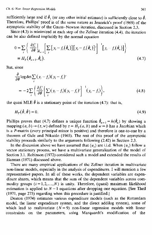
sufficiently large and if 4, (or any other initial estimate) is sufficiently close to 8. Therefore, Phillips’ proof is of the same nature as Jennrich’s proof (1969) of the asymptotic stability of the Gauss-Newton iteration, discussed in Section 2.3.

Since (4.3) is minimized at each step of the Zellner iteration (4.4), the iteration can be also defined implicitly by the normal equation

But, since

the quasi MLE 8 is a stationary point of the iteration (4.7): that is,

H,(e, 6) = 0. (4.9)

Phillips proves that (4.7) defines a unique function d,,+, = A(&) by showing a mapping (a, b) + (z, w) defined by z = Hr(a, b) and w = b has a Jacobian which is a P-matrix (every principal minor is positive) and therefore is one-to-one by a theorem of Gale and Nikaido (1965). The rest of this proof of the asymptotic stability proceeds similarly to the arguments following (2.42) in Section 2.3.

In the discussion above we have assumed that {u,} are i.i.d. When {u,} follow a vector stationary process, we have a’multivariate generalization of the model of Section 3.1. Robinson (1972) considered such a model and extended the results of Hannan (197 1) discussed above.

There are many empirical applications of the Zellner iteration in multivariate non-linear models, especially in the analysis of expenditures. I will mention a few representative papers. In all of these works, the dependent variables are expenditure shares, which means that the sum of the dependent variables across com- modity groups (i=1,2,..., N) is unity. Therefore, (quasi) maximum likelihood estimation is applied to N - 1 equations after dropping one equation. [See Theil (1971, page 275) regarding when this procedure is justified.]

Deaton (1974) estimates various expenditure models (such as the Rotterdam model, the linear expenditure system, and the direct addilog system), some of which lead to multivariate (N = 9) non-linear regression models with linear constraints on the parameters, using Marquardt’s modification of the

362 T. Amemiya

Gauss-Newton iteration to minimize (4.3) at each step of the Zellner iteration. Darrough (1977) estimates Diewert’s (1974) Generalized Leontief model with N = 4 and Berndt, Darrough and Diewert (1977) compare Translog [Christensen, Jorgenson and Lau (1975)], Generalized Leontief, and Generalized Cobb- Douglas [Diewert (1973)] models with N = 2. Both of these studies used some modification of the Gauss-Newton iteration to minimize (4.3). They are not explicit on this point except that they refer to Berndt, Hall, Hall and Hausman (1974).

In the expenditure analysis it is important to test various hypotheses on the form of the utility function (such as symmetry, homotheticity, and additivity). Also, if, as in the study of Deaton, different models can be nested in a single family, the choice of models can be done by a standard testing procedure. The above-mentioned studies use the likelihood ratio test to test these hypotheses. Deaton discusses the adequacy of the asymptotic &i-square distribution of the likelihood ratio test in these models and suggests the use of a simple multiplicative correction [Anderson (1958, pp. 207-210)].

Although it is not a Zellner iteration, I should also mention MacKinnon (1976), who estimated the S-branch utility model of Brown and Heien (1972) for the case of N = 6 by maximum likelihood estimation using the quadratic hill-climbing method, Powell’s conjugate gradient method, and the DFP method.

5. Simultaneous equations models

5.1. Non -linear two-stage least squares estimator

In this section we consider the non-linear regression equation

Y~=f(YIJ,dd+% t=1,2 ,..., T, (5.1)

where y, is a scalar endogenous variable, Y, is a vector of endogenous variables, X,, is a vector of exogenous variables, (me is a K-vector of unknown parameters, and (u,} are scalar i.i.d. random variables with Eu, = 0 and Vu, = cr*. The model does not specify the distribution of Y. Eq. (5.1) may be one of many structural equations which simultaneously define the distribution of y, and Y,, but here we are not concerned with the other equations. I will sometimes write f(y, Xu, (Ye) simply as f,(a,) or as f,. Also, I will define T-vectors y, f, and u in the same way I defined them in Section 2.1, and matrices Y and X,, whose t th rows are Y’ and Xi,, respectively.

The non-linear least squares estimator of (Y,, in this model generally yields an inconsistent estimator essentially for the same reason that the least squares estimator is inconsistent in a linear simultaneous equations model. We can see


this by considering (2.9) and noting that plim A, * 0 in general becausef, may be correlated with U, in the model (5.1) due to a possible dependence of Y, on u,. In this section I will consider how we can generalize the two-stage least squares (2SLS) method to the non-linear model (5.1) so that we can obtain a consistent estimator.

5.1.1. Non-linear only in parameters

The case where the non-linearity off occurs only in (~a does not pose much of a problem. Such a case will occur, for example, if the variables of a linear structural equation are transformed to take account of the autocorrelation of the error terms. The model which is nonlinear only in parameters can be written in vector form as

Y = Yu(&)+ X,PMJ+u. (5 -2)

We can generalize the two-stage least squares estimator in this model using either Theil’s interpretation of 2SLS [Theil (1953)] or the instrumental variables (I.V.) interpretation. Suppose the reduced form for Y is given by

y=xII+I/. (5.3)

If we use Theil’s interpretation, we should replace Y by Y = X( X’X)) ‘X’Y in the right-hand side of (5.2) and then apply the non-linear least squares estimation to (5.2). If we use the I.V. interpretation, we should premultiply (5.2) by X( X’X)) ‘X’ and then apply the non-linear least squares estimation. Clearly, we get the same estimator of 8, in either method. I will call the estimator thus obtained the non-linear two-stage least squares (NL2S) estimator of the model (5.2). In Amemiya (1974) it was proved that this NL2S estimator is asymptotically efficient in the model of (5.2) and (5.3); that is to say, it has the same asymptotic distribution as the maximum likelihood estimator of the same model (called the limited information maximum likelihood estimator). For an application of this estimator, see Zellner, Huang and Chau (1965).

5.1.2. Non -linear only in variables

Next, I consider the case wheref is non-linear only in variables. Let F,(Y,, X,) be a vector-valued function and let F be the matrix whose tth row is equal to F;. Then, the present case can be written as

y = Fy, + X,& + u. (5.4)

We will assume that the reduced form for 4 is not linear in X,, for then the model

364 T. Amemiya

is reduced to a linear model. Eq. (5.3) may or may not hold. This model is more problematical than the model (5.2). Here, the estimator obtained according to Theil’s interpretation is no longer consistent and the one based on the I.V. interpretation is consistent but no longer asymptotically efficient.

The following simple example illustrates why the application of Theil’s interpretation does not work in the present situation.’ Suppose a structural equation is

Y, = vz: + u, (5.5)

and is the reduced form for z1 is

z,=x,+u,. (5.6)

Note that I have simplified the matter by assuming that the reduced form coefficient is known. Inserting (5.6) into (5.5) yields

y,=yx,2+yu~+(U,+2yx,u,+yU~-yu,2), (5.7)

where the composite error term in parentheses has zero mean. Since the application of Theil’s interpretation to (5.5) means regressing y, on x: without a constant term, (5.7) clearly demonstrates that the resulting estimator is inconsistent.

That the estimator obtained according to the I.V. interpretation in the model (5.4) is not fully efficient can be seen by noting that the reduced form for Ft is not linear in X,. This suggests that one may hope to obtain a more efficient estimator by premultiplying (5.4) by W( W’W)- ‘W’, where the tth row of W, denoted W;, is a vector-valued function of X, such that the linear dependence of F, on W, is greater than that of F, on X,. Thus, in the present situation it is useful to consider the class of NL2S estimators with varying values for W. The elements of W, will be called instrumental variables.

Goldfeld and Quandt (1968) were the first to consider NL2S estimators in simultaneous equations models non-linear in variables. One of the two models they analyzed is given by9

log Y,, = Y, log Yzr + 8, + &t + ult, (5 -8)

Y2t = YZYI, + a+, + U2f * (5.9)

These equations constitute a whole simultaneous equations model, but I will

‘This statement should not be construed as a criticism of Theil’s interpretation. I know of at least six more interpretations of ZSLS: a certain interpretation works better than others when one tries to generalize 2SLS in a certain way. Thus, the more interpretations, the better.

9The subscript “0” indicating the true value is suppressed to simplify the notation.


consider only the estimation of the parameters of (5.8) for the time being. Note that in this model yZt does not have a linear reduced form like (5.3). Goldfeld and Quandt compared four estimators of (5.8) by a Monte Carlo study: (1) the least squares, (2) NL2S where W; = (1, x,), (3) NL2S where W; = (1, x,, xf), and (4) maximum likelihood.‘0 The ranking of the estimators turned out to be (2), (4), (3), and (1). However, the top ranking of (2) was later disclaimed by Goldfeld and Quandt (1972) as a computational error, since they found this estimator to be inconsistent. This was also pointed out by Edgerton (1972). In fact, the consistency of NL2S requires that the rank of W must be at least equal to the number of regression parameters to be estimated, as I will explain below. Goldfeld and Quandt (1968) also tried the Theil interpretation and discarded it since it gave poor results, as they expected.

Kelejian (1971) points out the consistency of the NL2S estimator using W of a sufficient rank and recommends that powers of the exogenous variables as well as the original exogenous variables be used as the instrumental variables to form W. Kelejian also shows the inconsistency of the estimator obtained by Theil’s interpretation. Edgerton (1972) also noted the consistency of NL2S. See Strickland and Weiss (1976) and Rice and Smith (1977) for applications of the NL2S estimator using Kelejian’s recommendation. The former estimates a three-equations model and the latter an eleven-equations model. Rice and Smith use other statistical techniques in conjunction with NL2S - a correction for the autocorrelation of the error terms and the use of principal components in the definition of W.

5.1.3. Non -linear in parameters and variables

Amemiya (1974) considered a general model (5.1) and defined the class of NL2S estimators as the value of (Y that minimizes

woo = (Y -f)‘w(w’w)-‘W’(y -r>, (5.10)

where W is some matrix of constants with rank at least equal to K. The minimization can be done using the iterative methods discussed in Section 2.3. The advantage of this definition is two-fold. First, it contains 2SLS and the NL2S estimators defined in the preceding two subsections as special cases. Second, and more importantly, the definition of the estimator as the solution of a minimization problem makes it possible to prove the consistency and the asymptotic

“Goldfeld and Quandt state that they generated U’S according to the normal distribution. But, their model is not well-defined unless the domain of U’S is somehow restricted. Thus, I must interpret the distribution they used as the truncated normal distribution. This means that the maximum likelihood derived under normality is not the genuine maximum likelihood.

366 T. Amemiya

normality of the NL2S estimator by standard techniques similar to the ones used in Section 2.2.

I will give an intuitive proof of the consistency by writing the expression corresponding to (2.9). [The method of proof used in Amemiya (1974) is slightly different.] Using a Taylor expansion of f(a) around (~c, we obtain the approximation

$sr(alW) = $dP wu + f (c-q, - a)‘G’Pwu

+~(a-a,)‘G’P,G(a-a,), (5.11)

where P, = W(W’W)- ‘W’ and G = (af/J(~‘),~. It is apparent from (5.11) that the consistency is attained if plim T- 'G'P,u = 0 and plim T- ‘G’P,G exists and has rank K. (Note that this implies that W must have at least rank K, which I assumed at the outset.) Intuitively it means that W should be chosen in such a way that the multiplication by P, eliminates all the part of G that is correlated with u but retains enough of it to make plim T- ‘G’P,G full rank.

The asymptotic normality of NL2S can be proved by a method analogous to the one used in Section 2.2 using formula (2.14). In the present case we have

3 aa ao

= - 2G’P,u

and

% = 2 plim; G’P,G.

Hence, if we denote the NL2S estimator by &:

(5.12)

(5.13)

(5.14)

Remember that I stated that the multiplication of G by P, should retain enough of G to make plimT_‘G’P,G full rank. The variance formula in (5.14) suggests that the more retained, the higher the efficiency.

Amemiya (1975) considered, among other things, the optimal choice of W. It is easy to show that plim T(G’P,G)- ’ is minimized in the matrix sense (i.e. A > B means A - B is a positive definite matrix) when one chooses W = EG. I will call the resulting estimator the best non-linear two-stage least squares estimator (BNL2S). Its asymptotic covariance matrix is given by

V, = a2plimT(EG’EG)-‘. (5.14)


However, BNL2S is not a practical estimator because of the following two problems: (1) it is often difficult to find an explicit expression for EG, and (2) EG generally depends on the unknown parameter vector q. The second problem is less serious since (Y,, may be replaced by any consistent member of the NL2S class using some W, such as that recommended by Kelejian (1971).

Given the first problem, the following procedure recommended by Amemiya (1976) seems the best practical way to approximate BNL2S. (1) Compute ai, a member of the NL2S class. (2) Evaluate G at &call it G. (3) Treat G as the dependent variables of regressions and search for the optimal set of independent variables, denoted W,, that best predict G. (4) Set W= We. (If we wanted to be more elaborate, we could search for a different set of independent variables for each column of G, say I#$ for the ith column &, and set W = [P,,g,, Pw,&, . . . ,

cvk&l.) Kelejian (1974) proposed another way to approximate EG. He proposed this

method for the model which is non-linear only in variables, but it could also work for certain fully non-linear cases. Let the tth row of G be Gi- that is, Gi = ( af,/&x’).O. Then, since G, is a function of Y, and q,, it is also a function of u, and q,; therefore, write G,( u,, a,,). Kelejian’s suggestion is to generate u, independently II times by simulation and approximate EG, by n-‘C:= ,G,( z+, a) when oi is some consistent estimator of (Y,,. Kelejian also points out that G,(O, 4) is also a possible approximation for EG,; although it is computationally simpler, it is likely to be a worse approximation than that given above.

Before Amemiya (1974), Tsurumi (1970) had actually used what amounted to the Gauss-Newton iteration to minimize (5.10). I overlooked this reference at the time of writing the 1974 article. In his article Tsurunii estimates the CES production function (2.3) by first linearizing the function around certain initial estimates of the parameters as in (2.38) and then proceeding as if he had the model which is nonlinear only in variables - the model of Section 5.1.2 above. The only difference between Tsurumi’s linearized function and (2.38) is that in Tsurumi’s case (af,/d/3’),j, is endogenous, since it contains L and K which are assumed to be endogenous variables in his model. Tsurumi tried two methods - the method according to Theil’s interpretation and the method according to the I.V. interpretation described in Section 5.1.2 above. In each method Tsurumi carried out the iteration until convergence occurred. Thus, the method according to the I.V. interpretation is actually the Gauss-Newton iteration to obtain NL2S. In the end Tsurumi discards the estimates obtained by the method according to Theil’s interpretation on the grounds that the convergence was slower and the estimates it produced were sometimes untenable. Tsurumi does not discuss the asymptotic properties of estimators derived by either method.

Hurd (1974) used a modification of NL2S to estimate the wage rate as a non-linear function of manhours, unemployment rate, and price level. His regression model has the form y = Z(A)cw + U, where many of the right-hand side

368 T. Amemiya

variables are transformed as z, - Xz,_ ,. He proposes transforming exogenous variables similarly, and minimizing [ y - Z( X)S]‘X( A)[ X( h)‘X( A)]- ‘X( h)‘[y - Z(X)01 with respect to X and 8 proves the consistency of the resulting NL2S estimator by a modification of the proof of Amemiya (1974).

5.1.4. Tests of hypotheses

I will consider the test of the hypothesis of the form

h(a) = 0, (5.15)

where h is a q-vector-valued non-linear function. Since we have not specified the distribution of all the endogenous variables of the model, we could not use the three tests defined in (2.54), (2.55), and (2.56), even if we assumed the normality of U. But we can use the following two test statistics: (1) the Wald test statistic analogous to (2.59), and (2) the difference between the constrained and the unconstrained sums of squared residuals (I will call it the SSRD test). Both statistics are based on the NL2S estimator 8. I will give the asymptotic distribution of the two statistics under the alternative hypothesis derived by Gallant and Jorgenson (1979). The normality of u is assumed.

I will assume that (5.15) can be alternatively written as

a=@), (5.16)

where 0 is a (K - q)-vector of freely varying parameters,” and write the asymptotic distribution in terms of both (5.15) and (5.16).

First, I will give a list of the symbols used in this section:

ai minimizes S,( aIW) without constraint,

~minimizesS,(crlW)subjecttoh(cu)=O,

~minimizesS,[~(8)lW]; therefore&==(#),

plim & = ‘Ye; plim is always taken under the model (5.1))

plim&==*,

ph8=e*; therefore cy* = r (e*),

(5.17)

“See Gallant and Jorgenson (1979, p. 299) for the conditions under which this is possible.

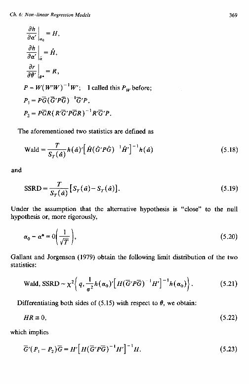
Ch. 6: Non -linear Regression Models

ah ad a0 = Hy

ah .. - aaf a;= Hy

ar a81 @. = R,

P=w(ww)-‘w’; I called this P, before; -- -

P, = PG(G’PG)-‘G’P,

P2 = PGR(R’G’PGR)-‘R@P.

The aforementioned two statistics are defined as

Wald = &h(b)‘[A(&Pi’)-%‘-lh(&)

369

(5.18)

and

SSRD = S,(&) --T-[&(a?)-S&q]. (5.19)

Under the assumption that the alternative hypothesis is “close” to the null hypothesis or, more rigorously,

a0 - (5.20)

Gallant and Jorgenson (1979) obtain the following limit distribution of the two statistics:

Wald, SSRD - x2( q, ~h(cto)‘[H(~‘P~)~‘H’]~‘h(cxo)). (5.21)

Differentiating both sides of (5.15) with respect to 8, we obtain:

HR=O,

which implies

(5.22)

G’( P, - P,)G = H’[ H(c’Pc)-‘H’] -‘H. (5.23)

310 T. Amemiya

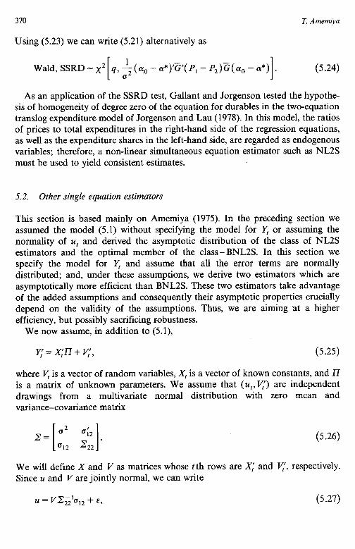
Using (5.23) we can write (5.21) alternatively as

Wald, SSRD - x2 q, $( a0 - a*)‘??( P, - P,)G( a0 - a*) . 1 (5.24)

As an application of the SSRD test, Gallant and Jorgenson tested the hypothesis of homogeneity of degree zero of the equation for durables in the two-equation translog expenditure model of Jorgenson and Lau (1978). In this model, the ratios of prices to total expenditures in the right-hand side of the regression equations, as well as the expenditure shares in the left-hand side, are regarded as endogenous variables; therefore, a non-linear simultaneous equation estimator such as NL2S must be used to yield consistent estimates.

5.2. Other single equation estimators

This section is based mainly on Amemiya (1975). In the preceding section we assumed the model (5.1) without specifying the model for Y, or assuming the normality of U, and derived the asymptotic distribution of the class of NL2S estimators and the optimal member of the class- BNL2S. In this section we specify the model for q and assume that all the error terms are normally distributed; and, under these assumptions, we derive two estimators which are asymptotically more efficient than BNL2S. These two estimators take advantage of the added assumptions and consequently their asymptotic properties crucially depend on the validity of the assumptions. Thus, we are aiming at a higher efficiency, but possibly sacrificing robustness.

We now assume, in addition to (5.1)

y= x;n+Fy, (5.25)

where V, is a vector of random variables, X, is a vector of known constants, and n is a matrix of unknown parameters. We assume that (u,, v:‘> are independent drawings from a multivariate normal distribution with zero mean and variance-covariance matrix

I= a2 42 I I cJl2 z . 22

(5.26)

We will define X and V as matrices whose t th rows are X,! and v, respectively. Since u and V are jointly normal, we can write

u = V&$7,, + E, (5.27)


where E is independent of V and distributed as N(0, u*~I), where Use = u 2 - 42Gh2.

The model defined above may be regarded either as a simplified non-linear simultaneous equations model in which both the non-linearity and the simultane- ity appear only in the first equation, or as the model that represents the “limited information” of the investigator. In the latter interpretation X, are not necessarily the original exogenous variables of the system, some of which appear in the arguments off, but, rather, are the variables a linear combination of which the investigator believes will explain Y, effectively.

5.2.1. Modified NL2S

In Section 5.1.3 we learned that the consistency of NL2S follows from the fact that the projection matrix, P,, removes the stochastic part of G, but that the “larger” P,G, the more efficient the estimator. This suggests that the projection matrix M, = I - V(V’V) -‘V’ should perform better than P, since it precisely eliminates the part of G that depends on V. Thus, if V were known (which is the same as if II were known), we could define the estimator that minimizes

(Y-mG(.Y-f). (5.28)

In order to verify the consistency of the estimator, write T -’ times the minimand in the same way as in (5.11). Then we get the same expression as the right-hand side of (5.1 l), except that P, is replaced by M,. Thus, the first condition for consistency is plim T -‘G’Myu = 0. But because of (5.27) this condition is equivalent to

plim+ G’M,e = 0. (5.29)

The above is generally satisfied if V and E are independent because G depends only on V. Note that here I have used the joint normality of u and V.12 Concerning the asymptotic efficiency, one can easily prove

plim f G’M,G 2 plim$ G’P,G (5.30)

for any constant W, so that this estimator is asymptotically more efficient than any member of the class of NL2S estimators.

12However, normality is not necessary. For example, it is sufficient to assume that u = Va + E for some (Y with V and E being independent.

372 T. Amemiya

However, since this estimator is not practical, I define the modified non-linear two-stage least squares estimator (MNL2Sj as the value of CY that minimizes (5.28) after replacing Y with Y - XZI, where ZI = (X’X) - ‘X’Y. Thus, MNL2S minimizes

(Y-f)l[Z-M,Y(Y’M,Y)_‘Y’M,](y-f), (5.31)

where M, = Z - X( X’X) -IX’. Its asymptotic covariance matrix is given in Amemiya (1975) as

V, = plimT(G’M,G)-‘[a*2G’M,G +(o* - a**)G’PxG](GfM,G)-‘,

(5.32)

where Px = X( X’X) - ‘X’. Amemiya (1975) proved

v,<v,. (5.33)

It is interesting to note that if f is linear in (Y and Y, MNL2S is reduced to the usual 2SLS.

5.2.2. Non -linear limited information maximum likelihood estimator (NLLZ)

Since the Jacobian of the transformation from (u, V) to (v, Y) is unity in our model, the log-likelihood function assuming normality can be written, apart from a constant, as

L** = - :loglz(-+trB-‘Q, (5.34)

where

u and V representing y - f and Y - XII, respectively. Solving aL**/d2 = 0 for 2 yields

z=+Q. (5.35)

Putting (5.35) into (5.34), we obtain a concentrated likelihood function

L* = - ; (logu’u +log(V’M,VI). (5.36)


Solving aL*/aII = 0 for IT, we obtain:

n= (x94,x)-'X'M,Y. (5.37)

Putting (5.37) into (5.36) yields a further concentrated likelihood function:

L= -~(logU’U+log,Y~M,Y-Y’M,x(x~~Ux)-’x’M,Y~), (5.38)

which depends only on (Y. Interpreting our model as that which represents the limited information of the researcher, I call the value of (Y that minimizes (5.38) the NLLI estimator. Its asymptotic covariance matrix is given by

It is proved in Amemiya (1975) that

v, < v,.

(5.39)

(5.40)

The maximization of (5.38) may be done by standard iterative procedures such as those discussed in Section 2.3. Another iterative method may be defined as follows. Rewrite (5.36) equivalently as

L* = - ; (log Z./M@ +log(v’vl) (5.41)

and iterate back and forth between (5.37) and (5.41). That is, obtain fi= (X’X) - ‘X’Y and v = Y - XI?, maximize (5.41) with respect to (Y after replacing V with t (at this point one gets the MNL2S estimator of (u), call this estimator ai and define fi = y - f(ai), insert it into (5.37) to obtain another estimator of IT, and repeat the procedure until convergence.

5.2.3. Comparison

In this and the preceding sections we have discussed four estimators: (1) NL2S (as a class), (2) BNL2S, (3) MNL2S, and (4) NLLI. If we denote NL2S(W= X) by SNLZS (the first S stands for standard), we have in the linear case

SNL2S = BNL2S = MNL2S a~ NLLI, (5.42)

where = means exact identity and z means asymptotic equivalence. In the non-linear model defined by (5.1) and (5.25) with the normality assumption we

374 T. Amemiya

have obtained the following ranking in terms of the asymptotic covariance matrix:

SNL2S + BNL2S < MNL2S < NLLI, (5.43)

where + means “is worse than”. However, it is important to remember that if the normality assumption is removed the last two estimators may lose consistency, whereas the first two estimators retain it.13

Quandt (1975) conducted a Monte Carlo experiment to study the comparative performance of several estimators, including those discussed above, in the following model:

Yl, = a, 1% Y2, + a2x1r + a3 + U1r

y2, = (X3t)n4.ht + a5X2t + ‘219

where ult and u2* are jointly normal.t4

(5.44)

(5.45)

Let us suppose that we want to estimate the parameters of (5.44), so that (5.44) is a specific example of (5.1). Then, there are two ways to define the reduced-form equation for y,,- the equation comparable to (5.25). How we define this equation determines SNL2S and NLFI. One way, which I think is the way Quandt adopted, is to define

y2, = rl + 7T2xI, + v3x2r + T4x3t + ‘f 7 (5.46)

and the other way is to define

Y2t = Tl + T2Xlr + =3x2t + T4x3t + 1T5x:, + %x;t

+ 7+x:, + 7rgx,rX2* + * * . + II,, (5.47)

where the right-hand side of (5.47) minus u, is a linear function of the x’s and the transformation of the x’s which the researcher believes best explains y21, subject to the condition that the number of parameters should not be so large.

We will assume that (5.46) is a specific example of (5.25); thus, SNL2S uses (1, x ,1, x2,, xgr) as v and NLLI is the maximum likelihood estimator applied to (5.44) and (5.46) assuming the joint normality of u,, and u,. Quandt compares the performance of ordinary least squares (OLS), SNL2S, the NL2S estimators where the W is chosen to be various sets of powers of the x’s, MNL2S, NLLI, and the full information maximum likelihood estimator (NLFI), which is the maximum

131n the simple model defined by (5.5) and (5.6), the necessary and sufficient condition for the consistency of either MNL2S or NLLI can be shown to be Eo2uEu2 = Eo3Euu.

14The same qualification as footnote 10 applies to this model as well.


likelihood estimator applied to the original equations (5.44) and (5.45). Quandt concludes that NLFI is the best, OLS is the worst, and the rest are more or less similar, although, to a certain extent, the asymptotic ranking (5.43) is preserved.

5.3. Non -hear simultaneous equations

So far I have considered the estimation of the parameters of a single equation in the system of simultaneous equations. Now, I will consider the estimation of all the parameters of the system.

The equations of the model are

fj(.YtY x,T aj> = Uiri i=1,2 T.--Y n; t=1,2 ,..., T, (5.48)

where yt is an n-vector of endogenous variables, x, is a vector of exogenous variables, and (Y~ is a &-vector of unknown parameters. I will assume that the n-vector ut = (u,~, uZt,. . . , unt)’ is an i.i.d. vector random variable with zero mean and variance-covariance matrix 2. Not all of the elements of the vectors y, and x, may actually appear in the arguments of each fi. I assume that each equation has its own vector of parameters (Y~ and that there are no constraints among the ai’s, but the results I state subsequently can easily be modified if we can express each (Y~ parametrically as ai( where the number of elements in 0 is fewer than CY=,Ki.

Strictly speaking, (5.48) is not a comIjlete model by itself because there is no guarantee that a unique solution for y, exists for every possible value of uit unless some stringent assumptions are made on the form of fi. Therefore, we will assume either that f, satisfies such assumptions or that if there is more than one solution for y, there is some additional mechanism by which a unique solution is chosen.

I have already mentioned two simple examples of (5.48): the model of Goldfeld and Quandt (1968), defined by (5.8) and (5.9), and the model of Quandt (1975), defined by (5.44) and (5.45). The first model is shown to possess two solutions occurring in two different regions; therefore, the model is not complete unless we specify some mechanism by which one of the two solutions is chosen. Goldfeld and Quandt conduct a Monte Carlo study in which they analyze how the performance of several estimators is affected by various mechanisms for choosing solutions such as always choosing solutions from one region or mixing solutions from two regions. [See Kelejian (1975) for a further study on this issue.] Quandt (1975) shows that in the second model above there is a one-to-one correspondence between y and u if it is assumed that (Y, < 0 and xgr > 0 for all t.

I will not discuss the problem of identification in the model (5.48). There are not many useful results in the literature beyond the basic discussion of Fisher (1966) as summarized in Goldfeld and Quandt (1972, p. 221 ff). I will merely

376 T. Amemiya

point out that non-linearity generally helps rather than hampers identification, so that, for example, the number of excluded exogenous variables in a given equation need not be greater than or equal to the number of parameters of the same equation in a non-linear model. I should also point out that I have actually given one sufficient condition for identifiability- that plim T - ‘(G’P,G) in the right-hand side of (5.14) be non-singular.

To facilitate the discussion of the subsequent sections I will give a list of symbols:

a= (c&a; ) . . . ) a;)‘,

A = 2~1, where @ is the Kronecker product,

fit =fi(Y,P x,, (yi), f, = an n-vector whose i th element is fi,,

Ai, = a T-vector whose t th element is fi,,

f = ( f(;, , f,;, , . . . ,.f,l,,)9 a nT-vecm

F= (f~l,,j&...,f~,,), a TXn-math

(5.49)

afit git = x 3 a &-vector,

‘f(i) Gi = a(y; , a T x Ki matrix whose t th row is gi:,

G=diag{G,,G, ,..., G,}, block diagonal matrix.

5.4. Non -linear three -stage least squares estimator

Before starting the main discussion I wish to point out that all the results of Sections 5.1 and 5.2 are valid if we change (5.1) to

Consequently, the minimand (5.10) which defines the class of NL2S estimators should be changed to

f’w(Fvw)-‘Wf. (5.51)

The asymptotic normality result (5.14) needs not be changed. The significance of


the above modification is that a NL2S estimator can be applied to each equation of (5.48)?

As a natural extension of the class of the NLZS estimators defined in Section 5.1.3, Jorgenson and Laffont (1974) defined the class of non-linear three-stage least squares estimators (NL3S) as the value of (Y that minimizes

f~[e-l@w(IVw)-‘W] f, (5.52)

where 2 is a consistent estimate of Z. For example,

e= f (5.53) t=l

where ai is the NL2S estimator obtained from each equation. The above definition is analogous to the definition of the linear 3SLS as a generalization of the linear 2SLS. The consistency and the asymptotic normality of the estimator defined above are proved in Jorgenson and Laffont (1974) and Gallant (1977).

The consistency of the NL2S and NL3S estimators of the parameters of the model (5.48) can be proved with minimal assumptions on uit- namely, those stated after (5.48). This robustness makes the estimators attractive. Another important strength of the estimators is that they retain their consistency regardless of whether or not (5.48) yields a unique solution for y, and, in the case of multiple solutions, regardless of what additional mechanism chooses a unique solution. See MaCurdy (1980) for an interesting discussion of this point.

Amemiya (1977) defined the class of the NL3S estimators slightly more generally as the value of (Y that minimizes

(5.54)

where h is a consistent estimate of A and S is a matrix of constants with nT rows and with the rank of at least cy_,K,. This definition is reduced to the Jorgenson-Laffont definition if S = diag( IV, IV,. . . , W). Its asymptotic variance- covariance matrix is given by

v, = plimT[G’A-‘S(S’A-‘S)-‘SW’G]-‘. (5.55)

Its lower bound is equal to

V’s, = limT[EG’A-‘EG]-‘, (5.56)

“Another advantage of this modification is that the Box-Cox transformation model (v: - 1)/h = B’x, + u, [see Box and Cox (1964)] can be regarded as a special case of (5.52). See Amemiya and Powell (I 980) for the application of NLZS to the Box-Cox model.

378 T. Amemiya

which is attained when one chooses S = EG. I will call this estimator the BNL3S estimator (B for best).

We can also attain the lower bound (5.56) using the Jorgenson-Laffont definition, but that is possible if and only if the space spanned by the column vectors of W contains the union of the spaces spanned by the column vectors of EG, for i = 1,2,. . _ , n. This necessitates including many columns in W, which is likely to increase the finite sample variance of the estimator although it has no effect asymptotically. This is a disadvantage of the Jorgenson-Laffont definition compared to my definition.

Noting that BNL3S is not practical just as BNL2S, Amerniya (1976) suggests the following approximation. (1) Compute Bi, an SNL2S estimator of q, i = 1,2,..., n. (2) Evaluate Gi at &,-call it &;. (3) Treat Gi as the dependent variables of the regression and search for the optimal set of independent variables K that best predict ei. (4) Choose S = diag{P,G,, P&, . . . , P,&,,}, where Pi = HgJq’~)-‘Fq’.

In Section 5.1.4 I discussed tests of hypotheses based on NL2S developed by Gallant and Jorgenson (1979). These tests can easily be generalized to the tests based on NL3S, as shown by the same authors.

Let B be the NL3S estimator here and let 2 be a consistent estimate of 2:. Also, let S,(a) refer to the NL3S minimand-and let d refer to the constrained NL3S subject to the condition (5.15) or (5.16). Then, the Wald and SSRD test statistics can now be defined as

Wald = h(~)‘{~[~‘(e-‘e~)~]-‘ri}-‘h(~), (5.57)

and

SSRD=S,(&)-S,(8), (5.58)

where G is G evaluated at ai and P = W(W’W)-‘W’. Note that (5.57) and (5.58) are similar to (5.18) and (5.19). The limit distribution of the two statistics under the alternative hypothesis (if it is “close” to the null hypothesis as before) is given by

Wald,SSRD-X2[4,h(aO)‘{~~[~‘(LI-1~P)G]H}-1h(cuo)], (5.59)

or, alternatively, using (5.22):

Wald, SSRD - x2 [q, ( a0 - a*)‘t?‘( P, - P2)c ( a0 - a*)],

where

(5.60)

P, = (X-‘~P)G[C’(Z-‘~P)G]-‘G’(X-‘eP)

319 Ch. 6: Non -linear Regression Models

and

P,=(Z-'OP)6R[R'~(Z-'OP)GR]-l~~~(~-'~P). As an application of the SSRD test, Gallant and Jorgenson tested the hypothe-

sis of symmetry of the matrix of parameters in the three-equation translog expenditure model of Jorgenson and Lau (1975).

The other applications of the NL3S estimators include Jorgenson and Lau [ 19781, which was previously mentioned in Section 5.1.4, and Haessel [ 19761, who estimated a system of demand equations, nonlinear only in parameters, by both NL2S and NL3S estimators.

5.5. Non -linear full information (NLFI) maximum likelihood estimator

In this section we consider the maximum likelihood estimator of model under the normality assumption of uit. To do so we must assume that

(5.48) (5.48)

defines a one-to-one correspondence between yt and u,. This assumption enables us to write down the likelihood function in the usual way as the product of the density of u, and the Jacobian. Unfortunately, this is a rather stringent assumption, which considerably limits the usefulness of the NLFI estimator in practice. We have already noted that Goldfeld and Quandt’s model defined by (5.8) and (5.9) does not satisfy this assumption. This example illustrates two types of problems which confront NLFI:

(1) Since there is no solution for y for some values of u, the domain of u must be restricted, which implies that the normality assumption cannot hold.

(2) Since there are two solutions for y for some values of u, one must specify a mechanism for choosing a unique solution in order to write down the likelihood function. One should note that the NL2S and the NL3S estimators are free from both of these problems.

Assuming u, - N(0, Z), we can write the log-likelihood function of the model (5.48) as

L*= - ;log]E]+ i log G -+ i f,lPh. II II t=l t t=1

Solving aL*/a_z = 0 for Z, we get:

E=+ 5 f,f,‘. r=l

(5.61)

(5.62)

Inserting (5.62) into (5.61) yields the concentrated log-likelihood function

L = Clog 3 - ;log]+f,f,‘]. II /I t

(5.63)

380 T. Amemiya

The NLFI maximum likelihood estimator of (Y is defined as the value of CY that maximizes (5.63).

It is shown in Amemiya (1977) that the NLFI estimator is consistent if the true distribution of u, is normal but is generally inconsistent if u, is not normal.‘6 This result is contrary to the result in the linear case where the FIML estimator derived from the normality assumption retains its consistency even if the true distribution is not normal. It is also shown in the same article that NLFI is asymptotically more efficient than BNL3S in general if the true distribution of U, is normal. (On the other hand, NL3S is more robust than NLFI because NL3S is consistent even if the distribution of U, is not normal.) This result is also contrary to the result in the linear case where FIML and 3SLS have the same asymptotic distribution. In the subsequent subsections I will further discuss these results as well as some other problems related to the NLFI estimator. I will not discuss hypotheses testing here since the discussion of Section 2.4.2 is applicable to the present model.

5.5.1. Consistency

Differentiating (5.63) with respect to (Y~, we obtain:

aL G-,=, 8%

- Ifi dgi, - Tt$, Sitf,‘(c.ftf,‘)~‘l, (5.64)

where (-)i ’ denotes the ith column of the inverse of the matrix within the parentheses. The consistency of NLFI is equivalent to the condition:

and hence to the condition:

(5.65)

(5.66)

where I# is the i th column of Z - ’ . Now, (5.66) could hold even if each term of a summation is different from the corresponding term of the other,‘but that event is extremely unlikely. Therefore, we can say that the consistency of NLFI is

“%k result is completely separate from and in no way contradicts the quite likely fact that the maximum likelihood estimator of a non-linear model derived under the assumption of a certain regular non-normal distribution is consistent if the true distribution is the same as the assumed distribution.


essentially equivalent to the condition:

agit EaUir = Egi,u;al. (5.67)

It is interesting to note that condition (5.67) holds if u, is normal because of the following lemma.17

Lemma

Suppose u = (u,, u2 ,..., u, )’ is distributed as N(0, Z), where 2 is positive definite. If ah(u)/&+ is continuous, E)ah/du,l -c GO, and ElhuJ <co, then

Eah =&Jai at+ 3 (5.68)

where u i is the i th column of 2 - I.

Another interesting question is: Does (5.67) hold even if u, is not normal? To throw some light on this question, let us suppose that the joint density of u, is Jl(u,), which may or may not be normal and that (5.65) holds where E is taken with respect to #(u,). If g,, and 4 satisfy certain conditions,‘* we have by integration by parts:

I~~(u)dui= -lgi~dui, I I

(5.69)

where I have suppressed the subscript t from g and u for simplicity. Integrating both sides of (5.69) with respect to the elements of u other than ui (this is not always permissible but we assume again that certain conditions on g and I/J enable us to do ~0)‘~ and combining the resulting equation with (5.69), we obtain:

A..@ ] + u’&//(u) gidu = 0. I

(5.70)

“This lemma, stated slightly differently, is originally due to Stein (1973). In Amemiya (1977), I rediscovered this lemma being unaware of Stein’s work. But, there was an error in the conditions of the lemma as presented in my article, which was pointed out by Phillips (1981). A correct proof is given in Amemiya (1981).

181f we treat ag./L$ and JI as functions of ui alone, it is sufficient to assume: (1) ag,/au, is continuous, (2) ~m~lagi/aail~dai < 00, and (3) #( .) . u, IS monotone decreasing for luil > M for some Mandlim,,,,,,$(ui)=O.

191t is sufficient if all the conditions of footnote 18 hold uniformly with respect to all the other elements of u.

382 T. Amemiya

Now, the question is: Does (5.70) hold for a density G(U) other than normal? The term within the square brackets in (5.70) is clearly zero if u is normal. Moreover, we can say “if and only if’ in the preceding sentence, provided that we restrict our attention to the class of continuously differentiable densities, 4, as proved by White (1980b). However, a#/&, + u’a’Jl(u) = 0 is not a necessary condition for (5.70) to hold, as we have noted in footnote 13 regarding a simple example of (5.5) and (5.6). This was first noted by Phillips (1981), who gives another interesting example. His model is defined by

1% Yl, + alx, = ult, (5.71)

Y21+ OLZYl, = U2t. (5.72)

In this example g, = 1 and g, = eU’-al; therefore, (5.70) clearly holds for i = 1 for any density $, and Phillips found a class of densities for which (5.70) holds for the case i = 2.

What is the significance of these examples? It is that given gi we can sometimes find a class of non-normal densities J/ for which (5.70) holds. When gi are simple, as in these examples, we can find a fairly broad class of non-normal densities for .which (5.70) holds. However, if gi is a more complicated non-linear function of the exogenous variables and the parameters {ai} as well as of u, (5.70) can be made to hold only when we specify a density which depends on the exogenous variables and the parameters of the model. In such a case, normality can be regarded, for all practical purposes, as a necessary and sufficient condition for the consistency of NLFI.

5.5.2. Comparison between NLFI and NL3S

Amemiya (1977) showed that the asymptotic equivalence of NLFI and BNL3S occurs if and (almost) only if fi, can be written in the form

~(Y,,x,,CWi)=Ai((Yi)‘Z(Yt,Xt)+Bi((Yi,Xt), (5.73)

where z is an n-vector of surrogate variables. Another instructive way to compare NLFI and BNL3S is to compare certain

iterative methods to obtain the two estimators. By equating the right-hand side of (5.64) to zero and rearranging terms we can

obtain the following iteration to obtain NLFI:

(5.74)


where

(5.75)

and & = diag(G,, G z, . . . , cn) and where all the variables that appear in the second term of the right-hand side of (5.74) are evaluated at ai(

The Gauss-Newton iteration to obtain BNL3S can be written as

(5.76)

where c; = EGI and G = diag(G,, G2,. . . ,G,) as before. Thus, we see that the only difference between (5.74) and (5.76) is in the

respective “instrumental variables” used in the formulae. Note that Gi defined in (5.75) can work as a proper set of “instrumental variables” (that is, the variables uncorrelated with ut) only if u, satisfies the condition of the aforementioned lemma, whereas ci is always a proper set of instrumental variables, which implies that BNL3S is more robust than NLFI. If u, is normal, however, Gi catches more of the part of Gi uncorrelated with u, than ci does, which implies that NLFI is more efficient than BNL3S under normality.

Note that (5.74) is a generalization of the formula expounded by Hausman (1975) for the linear case. Unlike in the linear case, however, the iteration defined by (5.74) does not have the property that ai is asymptotically equivalent to NLFI when oi(,) is consistent. Therefore, its main value may be pedagogical, and it may not be recommendable in practice.

5.5.3. Computation of NLFI

The discussion of the computation of NLFI preceded the theoretical discussion of the statistical properties of NLFI by more than ten years. The first paper on computation was by Eisenpress and Greenstadt (1966) who proposed a modified Newton-Raphson iteration. Their modification is the kind that combines both (2.28) and (2.29). Chow (1973) essentially differs from the above two authors in that he obtained simpler formulae by assuming that different parameters appear in different equations as in (5.48). I have already mentioned the iterative method considered by Amemiya (1977) mainly for a pedagogical purpose. Dagenais (1978) modified my iteration to speed up the convergence and compared it with a Newton-Raphson method due to Chow and Fair (1973) and the DFP iteration mentioned in Section 2.3.1 in certain examples of non-linear models. Results are inconclusive. Belsley (1979) compared the computation speed of the DFP iteration in computing NLFI and NL3S in five models of varying degrees of

384 T. Amemiya

complexity and found that NL3S was three to ten times faster. Nevertheless, Belsley shows that the computation of NLFI is quite feasible and can be improved by using a more suitable algorithm and by using the approximation of the Jacobian due to Fair- see eq. (5.79) below.

5.5.4. Other related papers

Fair and Parke (1980) estimated Fair’s (1976) macro model (97 equations, 29 of which are stochastic, with 182 parameters including 12 first-order autoregressive coefficients), which is non-linear in variables as well as in parameters (this latter non-linearity caused by the transformation to take account of the first-order autogression of the errors), by OLS, SNL2S, the Jorgenson-Laffont NL3S, and NLFI. The latter two estimators are calculated by a derivative-free algorithm due to Parke. This algorithm of NLFI uses the approximation of the Jacobian:

(5.79)

where J, = af,/i?y:, N is a small integer, and t,, t,,. . ., t, are equally spaced between 1 and T. Fair finds that in terms of predictive accuracy there is not much difference among different estimators, but in terms of policy response OLS is set apart from the rest.

Bianchi and Calzolari (1980) propose a method by which one can calculate the mean squared prediction error matrix of a vector predictor based on any estimator of the non-linear simultaneous equations model. Suppose the structural equations can be written as f ( yp, xp, a) = up at the prediction period p and we can solve it for yp as y, = g(x,, (Y, up). Define the predictor Yp based on the estimator B by $p = g(x,, &,O). (Note that yp is an n-vector.) Then we have

The authors suggest that A, be evaluated by simulation. As for A,, we can easily obtain its asymptotic value from the knowledge of the asymptotic distribution of ai.

Hatanaka (1978) considers a simultaneous equations model non-linear only in variables. Such a model can be written as F(Y, X)r + XB = U. Define P by F(?, X)f + X& = 0, where f and B are the OLS estimates. Then, Hatanaka proposes using F(p, X) as the instruments to calculate 3SLS. He proposes the


method-of-scoring iteration to calculate NLFI where the iteration is started at the aforementioned 3SLS. He also proves the consistency and the asymptotic normality of NLFI and obtains its asymptotic covariance matrix [which can be also obtained from Amemiya (1977) by an appropriate reduction].

References

Akaike, H. ( 1973) “ Information Theory and an Extension of the Maximum Likelihood Principle”, in: B. N. Petrov and F. Csaki (eds.), Second International Symposium on Information Theory. Budapest: Akademiai Kiado, pp. 267-28 1.

Amemiya, T. (1973a) “Generalized Least Squares with an Estimated Autocovariance Matrix”, Econometrica, 41, 723-732.

Amemiya, T. (1973b) “Regression Analysis When the Dependent Variable Is Truncated Normal”, Econometrica, 41, 997- 1016.

Amemiya, T. (1974) “The Nonlinear Two-Stage Least-Squares Estimator”, Journal of Econometrics, 2, 105- 1 IO.

Amemiya, T. (1975) “The Nonlinear Limited-Information Maximum-Likelihood Estimator and the Modified Nonlinear Two-Stage Least-Squares Estimator”, Journal of Econometrics, 3, 375-386.

Amemiya, T. (1976) “Estimation in Nonlinear Simuhaneous Equation Models”, Paper presented at Institut National de La Statistique et Des Etudes Economiques, Paris, March 10 and published in French in: E. Malinvaud (ed.), Cahiers Du Seminaire D ‘econometric, no. 19 (I 978).

Amemiya, T. (1977) “The Maximum Likelihood and the Nonlinear Three-Stage Least Squares Estimator in the General Nonlinear Simultaneous Equation Model”, Econometrica, 45, 955-968.

Amemiya, T. (I 980) “Lecture Notes in Advanced Theory of Econometrics”, Department of Econom- ics, Stanford University.

Amemiya, T. ( 198 1) “ Correction to a Lemma”, forthcoming in Econometrica. Amemiya, T. and W. A. Fuller (1967) “A Comparative Study of Alternative Estimators in a

Distributed Lag Model”, Econometrica, 35, 509-529. Amemiya, T. and J. L. Powell (1980) “A Comparison of the Box-Cox Maximum Likelihood Estimator

and the Nonlinear Two Stage Least Squares Estimator”, Technical Report No. 322, August, Institute for Mathematical Studies in the Social Sciences, Stanford University.

Anderson, T. W. (1958) An Introduction to Multivariate Statistical Analysis. New York: John Wiley & sons.

Anderson, T. W. (1971) The Statistical Analysis of Time Series. New York: John Wiley & Sons. Arrow. K. J.. H. B. Chenerv. B. S. Minhas and R. M. Solow (1961) “Capital-Labor Substitution and

Ecohomic’Efficiency”, R-&iew of Economics and Statististics, 43,‘225-250. Bard, Y. (1974) Nonlinear Parameter Estimation. New York: Academic Press. Bates. D. M. and D. G. Watts (1980) “Relative Curvature Measures of Nonlinearitv”. Journal of the

Royal Statistical Society, Ser. ‘B, 42, 1-25 (with discussion). _

Beale, E. M. L. (1960) “Confidence Regions in Non-Linear Estimation”, Journal of the Royal Statistical Society, Ser. B, 22, 41-88 (with discussion).

Beauchamp, J. J. and R. G. Cornell (1966) “Simultaneous Nonlinear Estimation”, Technometrics, 8, 3 19-326.

Belsley, D. A. (1979) “On the Computational Competitiveness of Full-Information Maximum-Likeh- hood and Three-Stage Least-Squares in the Estimation of Nonlinear Simultaneous-Equations Models”, Journal of Econometrics, 9, 3 15-342.

Bemdt, E. R., W. E. Diewert and M. N. Darrough (1977) “Flexible Functional Forms and Expenditure Distributions: An Application to Canadian Consumer Demand Functions”, Interna- tional Economic Review, 18, 65 I-676.

Bemdt, E. R., B. H. Hall, R. E. Hall and J. A. Hausman (1974) “Estimation and Inference in Nonlinear Structural Models”, Annals of Econometric and Social Measurement, 3, 653-666.

Bemdt, E. R. and N. E. Savin (1977) “Conflict Among Criteria for Testing Hypotheses in the Multivariate Linear Regression Model”, Econometrica, 45, 1263- 1278.

386 T. Amemiya

Bianchi, C. and G. Calzolari (1980) “The One-Period Forecast Error in Non-linear Econometric Models”, International Economic Review, 21, 201-208.

Bodkin, R. G. and L. R. Klein (1967) “Nonlinear Estimation of Aggregate Production Functions”, Review of Economics and Statistics, 49, 28-44.

Box, G. E. P. and D. R. Cox (1964) “An Analysis of Transformations”, Journal of Royal Statistical Society, Ser. B, 26, 21 l-252 (withdiscussion):

_ _

Brown. M. and D. Heien (1972) “The S-Branch Utilitv Tree: A Generalization of the Linear Expenditure System”, Econometrica, 40, 737-747. _

But&e, H., K. Henscheke, R. Sttiiby and C. Wisotzki (1977) “Parameter Estimation in Nonlinear Regression Models”, Mathematische Operationsforschung und Statistik, Series Statistics, 8, 23-40.

Charatsis, E. G. (1971) “A Computer Program for Estimation of the Constant Elasticity of Substitu- tion Production Function”, Applied Statistics, 20, 286-296.

Chow. G. C. (1973) “On the Comnutation of Full-Information Maximum Likelihood Estimates for Nonlinear Equation Systems”, R&-w of Economics and Statistics, 55, lCl- 109.

Chow, G. C. and R. C. Fair (1973) “Maximum Likelihood Estimation of Linear Equation Systems with Auto-Regressive Residuals”, Annals of Economic and Social Measurement, 2, 17-28.

Christensen, L. R., D. W. Jorgenson and L. J. Lau (1975) “Transcendental Logarithmic Utility Functions”, American Economic Review, 65, 367-383.

Cox, D. R. ( 196 1) “Tests of Separate Families of Hypotheses”, in: J. Neyman (ed.), Proceedings of the Fourth Berkeley Symposium on Mathematical Statistics and Probability, vol. I. Berkeley: University of California Press, pp. 105-123.

Cox, D. R. (1962) “Further Results on Tests of Separate Families of Hypotheses”, Journal of the Royal Statistical Society, Ser. B, 24, 406-424.

Dagenais, M. G. (1978) “The Computation of FIML Estimates as Iterative Generalized Least Squares Estimates in Linear and Nonlinear Simultaneous Eouations Models”, Econometrica. 46, 1351-1362.

Darrough, M. N. (1977) “A Model of Consumption and Leisure in an Intertemporal Framework: A Systematic Treatment Using Japanese Data”, International Economic Review, i8, 677-696.

Davidon. W. C. (19591 “Variable Metric Method for Minimization”, AEC Research Development Report, ANL-5990. ’

Deaton, A. S. (1974) “The Analysis of Consumer Demand in the United Kingdom, 1900- 1970”, Econometrica, 42, 341-368.

Diewert, W. E. (1973) “Separability and a Generalization of the Cobb-Douglas Cost, Production, and Indirect Utility Functions”, Technical Report 86, January, Institute for Mathematical Studies in the Social Sciences, Stanford University.

Diewert, W. E. (1974) “Applications of Duality Theory”, in: M. Intriligator and D. Kendrick (eds.), Frontiers of Quantitative Economics, vol. II. Amsterdam: North-Holland Publishing Co., pp. 106-171.

Draper, N. R. and H. Smith (1966) Applied Regression Analysis. New York: John Wiley & Sons. Edgerton, D. L. (1972) “Some Properties of Two Stage Least Squares as Applied to Non-Linear

Models”, International Economic Review, 13, 26-32. Eisenpress, H. and J. Greenstadt (1966) “The Estimation of Nonlinear Econometric Systems”,

Econometrica, 34, 85 1-86 1. Fair, R. C. (1976) A Model of Macroeconomic Activity, Vol. II: The Empirical Model. Cambridge,

Mass.: Ballinger. Fair, R. C. and W. R. Parke (1980) “Full-Information Estimates of a Non-linear Macroecometric

Model”, Journal of Econometrics, 13, 269-291. Fisher, F. M. (1966) The Identification Problem in Econometrics. New York: McGraw-Hill. Fletcher. R. and M. J. D. Powell (1963) “A Ranidlv Convereent Descent Method for Minimization”.

Computer Journal, 6, 163-168. ~ ’ A * - Gale, D. and H. Nikaido (1965) “The Jacobian Matrix and Global Univalence of Mappings”,

Mathematische Annalen, 159, 81-93. Gallant, A. R. (1975a) “Nonlinear Regression”, The American Statistician, 29, 73-81. Gallant, A. R. (1975b) “The Power of the Likelihood Ratio Test of Location in Nonlinear Regression

Models”, Journal of the American Statistical Association, 70, 198-203. Gallant, A. R. (1975~) “Testing a Subset of the Parameters of a Nonlinear Regression Model”,

Journal of the American Statistical Association, 70, 927-932.


Gallant, A. R. (1975d) “Seemingly Unrelated Nonlinear Regression”, Journal of Econometrics, 3, 35-50.

Gallant, A. R. (1977) “Three-Stage Least-Squares Estimation for a System of Simultaneous, Nonlin- ear, Implicit Equations”, Journal of Econometrics, 5, 71-88.

Gallant, A. R. and J. J. Goebel (1976) “Nonlinear Regression with Autocorrelated Errors”, Journal of the Americun Stutisticul Association, 7 1, 96 l-967.

Gallant, A. R. and A. Holly (1980) “Statistical Inference in an Implicit, Nonlinear, Simultaneous Equation Model in the Context of Maximum Likelihood Estimation”, Econometrica, 48, 697-720.

Gallant, A. R. and D. W. Jorgenson (1979) “Statistical Inference for a System of Simultaneous, Non-Linear, Implicit Equations in the Context of Instrumental Variable Estimation”, Journal of Econometrics, 11, 275-302.

Glasbey, C. A. (1979) “Correlated Residuals in Non-Linear Regression Applied to Growth Data”, Applied Statistics, 28, 25 l-259.

Guttman, I. and D. A. Meeter (1965) “On Beale’s Measures of Non-Linearity”, Technometrics, 7, 623-637.

Goldfeld, S. M. and R. E. Quandt (1968) “Nonlinear Simultaneous Equations: Estimation and Prediction”, International Economic Review, 9, 113- 136.

Goldfeld, S. M. and R. E. Quandt (1972) Nonlinear Methods in Econometrics. Amsterdam: North-Hol- land Publishing Co.

Goldfeld, S. M., R. E. Quandt and H. F. Trotter (1966) “Maximization by Quadratic Hill-Climbing”, Econometrica, 34, 541-551.

Haessel, W. (1976) “Demand for Agricultural Commodities in Ghana: An Application of Nonlinear Two-Stage Least Squares with Prior Information”, American Journal of Agricultural Economics, 58, 341-345.

Hannan, E. .I. (1963) “Regression for Time Series”, in: M. Rosenblatt (ed.), Time Series Analysis. New York: John Wiley & Sons, pp. 17-37.

Hannan, E. J. (1971) “Non-Linear Time Series Regression”, Journal of Applied Probability, 8, 767-780.

Hartley, H. 0. (1961) “The Modified Gauss-Newton Method for the Fitting of Non-Linear Regres- sion Functions By Least Squares”, Technometrics, 3, 269-280.

Hartley, H. 0. (1964) “Exact Confidence Regions for the Parameters in Non-Linear Regression Laws”, Biometrika, 5 1, 347-353.

Hartley, H. 0. and A. Booker (1965) “Non-Linear Least Squares Estimation”, Annuls of Mathematical Statistics, 36, 638-650.

Hatanaka, M. (1978) “On the Efficient Estimation Methods for the Macro-Economic Models Nonlinear in Variables”, Journal of Econometrics, 8, 323-356.

Hausman, J. A. (1975) “An Instrumental Variable Approach to Full Information Estimators for Linear and Certain Nonlinear Econometric Models”, Econometrica, 43, 727-738.

Hildreth, C. and J. P. Houck (1968) “Some Estimators for a Linear Model with Random Coefficients”. Journal of the American Statistical Association, 63, 584-595.

Hoadley, B. (197 1) “Asymptotic Properties of Maximum Likelihood Estimators for the Independent Not Identically Distributed Case”, Annuls of Mathematical Statistics, 42, 1977-1991.

Howe, H., R. A. Pollack and T. J. Wales (1979) “Theory and Time Series Estimation of the Quadratic Expenditure System”, Econometrica, 47, 123 1- 1248.

Hurd, M. D. (1974) “Wage Changes, Desired Manhours and Unemployment”, Memorandum No. 155 (Revised), October, Center for Research in Economic Growth, Stanford University.

Jennrich, R. I. (1969) “Asymptotic Properties of Non-linear Least Squares Estimation”, Annals of Mathematical Statistics, 40, 633-643.

Jorgenson, D. W. and J. Laffont (1974) “Efficient Estimation of Nonlinear Simultaneous Equations with Additive Disturbances”, Annals of Economic and Social Measurement, 3, 615-640.

Jorgenson, D. W. and L. J. Lau (1975) “The Structure of Consumer Preferences”, Annuls of Economic and Social Measurement, 4, 49-101.

Jorgenson, D. W. and L. J. Lau (1978) “Testing the Integrability of Consumer Demand Functions, United States, 1947-1971”, mimeo.

Judge, G. G., W. E. Griffiths, R. C. Hill and T. C. Lee (1980) The Theory and Practice of Econometrics. New York: John Wiley & Sons.

388 T. Amemiya

Just, R. E. and R. D. Pope (1978) “Stochastic Specification of Production Functions and Economic Implications”, Journal of Econometrics, 7, 67-86.

Kelejian, H. H. (1971) “Two-Stage Least Squares and Econometric Systems Linear in Parameters but Nonlinear in the Endogenous Variables”, Journal of the American Statistical Association, 66, 373-374.

Kelejian, H. H. (1974) “Efficient Instrumental Variable Estimation of Large Scale Nonlinear Econometric Models”, mimeo.

Kelejian, H. H. (1975) “Nonlinear Systems and Non-Unique Solutions: Some Results Concerning Estimation”, mimeo., May (Revised).

MacKinnon, J. G. (1976) “Estimating the Linear Expenditure System and Its Generalizations”, in: S. M. Goldfeld and R. E. Quandt (eds.), Studies in Nonlinear Estimation. Cambridge, Mass.: Ballinger, pp. 143- 166.

MaCurdy, T. E. (1980) “An Intertemporal Analysis of Taxation and Work Disincentives”, Working Papers in Economics no. E-80-4, The Hoover Institution, Stanford University.

Malinvaud, E. (1970a) “The Consistency of Nonlinear Regressions”, Annals of Mathematical Statis- tics, 41, 956-969.

Malinvaud, E. (I 970b) Statistical Methodr of Econometrics (2nd rev. edn.). Amsterdam: North-Holland Publishing Co.

Marquardt, D. W. (1963) “An Algorithm for Least Squares Estimation of Nonlinear Parameters”, Journal of the Society for Industrial and Applied Mathematics, 11, 43 l-441.

Mizon, G. E. (1977) “Inference Procedures in Nonlinear Models: An Application in a UK Industrial Cross Section Study of Factor Substitution and Returns to Scale”, Econometrica, 45, 1221-1242.

Phillips, P. C. B. (1976) “The Iterated Minimum Distance Estimator and the Quasi-Maximum Likelihood Estimator”, Econometrica, 44, 449-460.

Phillips, P. C. B. (1981) “On the Consistency of Non-Linear FIML”, mimeo. Poirier, D. .I. (1976) The Econometrics of Structural Change. Amsterdam: North-Holland Publishing

co. Powell, M. J. D. (1964) “A Efficient Method for Finding the Minimum of a Function of Several

Variables Without Calculating Derivatives”, Computer Journal, 7, 115- 162. Priestley, M. B. (I 978) “Non-Linear Models in Time Series Analysis”, The Statistician, 27, 159- 176. Quandt, R. E. (1975) “A Note on Amemiya’s Nonlinear Two-Stage Least Squares Estimators”,

Research Memorandum no. 178, May, Econometric Research Program, Princeton University. Rao, C. R. (1947) “Large Sample Tests of Statistical Hypotheses Concerning Several Parameters with

Applications to Problems of Estimation”, Proceedings of Cambridge Philosophical Society, 44, 50-57. Rao, C. R. (1973) Linear Statistical Inference and Its Applications (2nd edn.). New York: John Wiley &

Sons. Revankar, N. S. (1971) “A Class of Variable Elasticity of Substitution Production Function”,

Econometrica, 39, 6 1-7 1. Rice, P. and .V. K. Smith (1977) “An Econometric Model of the Petroleum Industry”, Journal of

Econometrics, 6. 263-288. Robinson, P. M. (1972) “Non-Linear Regression for Multiple Time-Series”, Journal of Applied

Probability, 9, 758-768. Sargent, T. J. (I 978) “Estimation of Dynamic Labor Demand Schedules Under Rational Expectations”,

Journal of Political Economy, 86, 1009- 1044. Silvey, S. D. (1959) “The Lagrangian Multiplier Test”, Annals of Mathematical Statistics, 30, 389-407. Stein, C. (1973) “Estimation of the Mean of a Multivariate Normal Distribution”, Technical Report

no. 48, June 26, Department of Statistics, Stanford University. Strickland, A. D. and L. W. Weiss (1976) “Advertising, Concentration, and Price-Cost Margins”,

Journal of Political Economy, 84, 1109-l 121. Theil, H. (1953) “Repeated Least-Squares Applied to Complete Equation Systems”, mimeo. The

Hague: Central Planning Bureau. Theil, H. (1971) Principles of Econometrics. New York: John Wiley 8~ Sons. Tornheim, L. (1963) “Convergence in Nonlinear Regression”, Technometrics, 5, 5 13-5 14. Tsurumi, H. (1970) “Nonlinear Two-Stage Least Squares Estimation of CES Production Functions

Applied to the Canadian Manufacturing Industries”, Reoiew of Economics and Statistics, 52, 200-207.


Wald, A. (1943) “Tests of Statistical Hypotheses Concerning Several Parameters When the Number of Observations is Large”, Transaction of American Mathematical Society, 54, 426-482.

Wald, A. (1949) “Note on the Consistency of the Maximum Likelihood Estimate”, Annals of Mathematical Statistics, 60, 595-601.

White, H. (1980a) “Nonlinear Regression on Cross-Section Data”, Econometrica, 48, 721-746. White, H. (1980b) “A Note on Normality and the Consistency of the Nonlinear Simultaneous

Equations Maximum Likelihood Estimator”, May, mimeo. Wolter, K. M. and W. A. Fuller (1978) “Estimation of Nonlinear Errors-in-Variables Models”,

mimeo. Wu, C. F. (I 98 I) “Asymptotic Theory of Nonlinear Least Squares Estimation”, Annals of Stafisfics, 9,

501-513. Zellner, A. (1962) “An Efficient Method of Estimating Seemingly Unrelated Regressions and Tests for

Aggregation Bias”, Journal of the American Statisfical Association, 57, 348-368. Zellner, A., D. S. Huang and L. C. Chau (1965) “Further Analysis of the Short-Run Consumption

Function with Emphasis on the Role of Liquid Assets”, Econometrica, 33, 571-581.

Documents

NON-LINEAR REGRESSION MODELS - VirtualPanicvirtualpanic.com/anonymousftplistings/ebooks/ECONOMICS/Amemiya...Single equation-i.i.d. case 2.1. Model ... Non -linear Regression Models