Embed Size (px)
Citation preview

NOAA Technical Report NWS 53
Modification of Sacramento Soil Moisture Accounting Heat Transfer Component (SAC-HT) for Enhanced Evapotranspiration Victor Koren Michael Smith Zhengtao Cui Brian Cosgrove Kevin Werner Robert Zamora October 2010 U.S. DEPARTMENT OF COMMERCE National Oceanic and Atmospheric Administration National Weather Service

NOAA Technical Report NWS 53 October 2010 ii
This page intentionally left blank
Office of Hydrologic Development (OHD) SCIENCE TECHNICAL REPORT
For
Modification of Sacramento Soil Moisture Accounting Heat Transfer Component (SAC-HT) for
Enhanced Evapotranspiration
Victor Koren and Michael Smith NOAA, NWS, Office of Hydrologic Development
Kevin Werner
NOAA, NWS, Colorado Basin River Forecast Center
Robert Zamora NOAA, Earth System Research Laboratory
Results presented at OHD Seminar August 26, 2010
Final report approved by OHD October 13, 2010

NOAA Technical Report NWS 53 October 2010 iv
A partial listing of recent reports in this series
NWS 50 Distributed Modeling: Phase 1 Results. Michael Smith, Victor Koren, Bryce Finnerty, Dennis Johnson. February, 1999 NWS 51 NOAA NWS Distributed Hydrologic Modeling Research and Development. Michael Smith, Victor Koren, Ziya Zhang, Seann Reed, Dongjun Seo, Fekadu Moreda, Vadim Kuzmin, Zhengtao Cui, Richard Anderson. April, 2004 NWS 52 Physically-Based Modifications to the Sacramento Soil Moisture Accounting Model: Modeling the Effects of Frozen Ground on the Rainfall-Runoff Process. Victor Koren, Michael Smith, Zhengtao Cui, Brian Cosgrove. July, 2007

NOAA Technical Report NWS 53 October 2010 v
Table of Contents
1. Introduction 1
2. Problem description 2
3. SAC-HT modification approach 3
3.1. Formulation of SAC-HT water exchange mechanism 4
3.2. Implementation of canopy resistance parameterization 8
3.3. Changes to the Noah parameterization to reduce input data
requirements 10
3.4. Parametric data 15
3.5. Changes to Noah root zone definition 17
4. Test results 17
4.1. Point-type application 18
4.2. Lumped basins application 27
5. Research findings 52 6. Conclusions 54
7. Recommendations 54
8. References 56
9. Attachment: Literature review 58

NOAA Technical Report NWS 53 October 2010 vi
This page intentionally left blank

NOAA Technical Report NWS 53 October 2010 1
1. Introduction SAC-SMA also has no controls on the movement of water to satisfy evaporation. In SAC-SMA if the potential evaporation rate is not satisfied from the upper storage, it will withdraw water directly from lower storages. As a result, the soil moisture of the SAC-SMA lower zone may be underestimated considerably in dry basins. Furthermore, SAC-SMA does not account well for the effects of vegetation. Vegetation transpires water drawn from various soil layers based on its root depth, root distribution and its resistance to transpiration demand. Under severely dry conditions, the upper layer soil moisture and part of the lower layer can be even more underestimated because the vegetation resistance and the source of transpiration withdrawals are not considered. Recently, the SAC-SMA was enhanced by incorporating a heat transfer component, resulting in the SAC-HT version. SAC-HT accounts for soil moisture and soil temperature at different physical rather than conceptual soil layers. However, it continues to suffer from the same lack of canopy resistance as described above for SAC-SMA. Test results for the Oklahoma Mesonet basins (Koren et al., 2006) support the observation of the evapotranspiration deficiency of the SAC-SMA and SAC-HT, e.g., Fig. 1.1.
Figure 1.1. Runoff and lower zone soil moisture bias for Oklahoma Mesonet river basins
The goal of this project is to reduce the deficiency of SAC-HT by incorporating an advanced definition of the canopy resistance parameterization developed in land surface models and used in the operational Noah model. To be compatible with the SAC-HT structure and input data requirements, the canopy resistance formulation will be reduced to be usable with only air temperature data. It will allow using the new SAC-HT model with the River Forecast Centers’ (RFCs) currently available operational meteorological input data. The new SAC-HT will improve the accuracy of the simulation/prediction of river runoff and soil moisture. The new
Fractional runoff volume bias
0
0.5
1
1.5
2
2.5
0.2 0.4 0.6 0.8
Climate index
Runo
ff bi
as
Lower layer soil moisture bias
-0.2
-0.15
-0.1
-0.05
0
0.05
0.1
0.2 0.4 0.6 0.8
Climate index
Soil
moi
stur
e bi
as
NOAA Technical Report NWS 53 October 2010 2
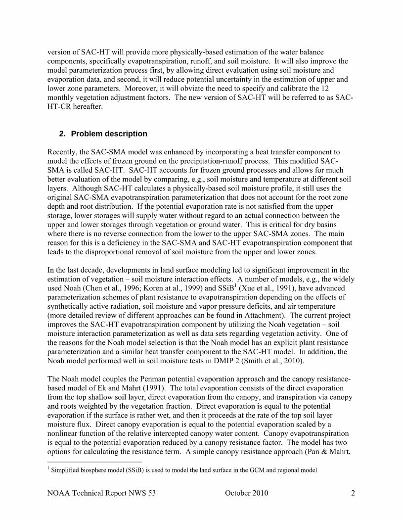
version of SAC-HT will provide more physically-based estimation of the water balance components, specifically evapotranspiration, runoff, and soil moisture. It will also improve the model parameterization process first, by allowing direct evaluation using soil moisture and evaporation data, and second, it will reduce potential uncertainty in the estimation of upper and lower zone parameters. Moreover, it will obviate the need to specify and calibrate the 12 monthly vegetation adjustment factors. The new version of SAC-HT will be referred to as SAC-HT-CR hereafter.
2. Problem description Recently, the SAC-SMA model was enhanced by incorporating a heat transfer component to model the effects of frozen ground on the precipitation-runoff process. This modified SAC-SMA is called SAC-HT. SAC-HT accounts for frozen ground processes and allows for much better evaluation of the model by comparing, e.g., soil moisture and temperature at different soil layers. Although SAC-HT calculates a physically-based soil moisture profile, it still uses the original SAC-SMA evapotranspiration parameterization that does not account for the root zone depth and root distribution. If the potential evaporation rate is not satisfied from the upper storage, lower storages will supply water without regard to an actual connection between the upper and lower storages through vegetation or ground water. This is critical for dry basins where there is no reverse connection from the lower to the upper SAC-SMA zones. The main reason for this is a deficiency in the SAC-SMA and SAC-HT evapotranspiration component that leads to the disproportional removal of soil moisture from the upper and lower zones. In the last decade, developments in land surface modeling led to significant improvement in the estimation of vegetation – soil moisture interaction effects. A number of models, e.g., the widely used Noah (Chen et al., 1996; Koren at al., 1999) and SSiB1 (Xue et al., 1991), have advanced parameterization schemes of plant resistance to evapotranspiration depending on the effects of synthetically active radiation, soil moisture and vapor pressure deficits, and air temperature (more detailed review of different approaches can be found in Attachment). The current project improves the SAC-HT evapotranspiration component by utilizing the Noah vegetation – soil moisture interaction parameterization as well as data sets regarding vegetation activity. One of the reasons for the Noah model selection is that the Noah model has an explicit plant resistance parameterization and a similar heat transfer component to the SAC-HT model. In addition, the Noah model performed well in soil moisture tests in DMIP 2 (Smith et al., 2010). The Noah model couples the Penman potential evaporation approach and the canopy resistance-based model of Ek and Mahrt (1991). The total evaporation consists of the direct evaporation from the top shallow soil layer, direct evaporation from the canopy, and transpiration via canopy and roots weighted by the vegetation fraction. Direct evaporation is equal to the potential evaporation if the surface is rather wet, and then it proceeds at the rate of the top soil layer moisture flux. Direct canopy evaporation is equal to the potential evaporation scaled by a nonlinear function of the relative intercepted canopy water content. Canopy evapotranspiration is equal to the potential evaporation reduced by a canopy resistance factor. The model has two options for calculating the resistance term. A simple canopy resistance approach (Pan & Mahrt, 1 Simplified biosphere model (SSiB) is used to model the land surface in the GCM and regional model
NOAA Technical Report NWS 53 October 2010 3
1987) is based on a constant ‘plant coefficient’ scaled by a soil moisture stress function. The soil moisture stress function is calculated as a relative value of available soil moisture in the range between field capacity and wilting point. A more advanced approach accounts for several different stress factors. It accounts for the effects of photosynthetically active radiation, soil moisture and vapor pressure deficits, and air temperature. The model has a number of parameters which need to be defined using soil and vegetation properties. The simple canopy resistance approach requires 10 parameters (six of them are used in derivation of a priori SAC-HT parameters), and the advanced approach requires 5 more parameters. Fortunately, a priori parameter grids exist over the Continental United States (CONUS) for most model parameters from the National Center for Environmental Prediction (NCEP) at the Hydrologic Rainfall Analysis Project (HRAP) resolution. Based on physical reasoning and available publications on Noah model results, the advanced canopy resistance parameterization was utilized. The most critical consideration is input data requirements. The Noah model, like most land surface models, requires considerable input data such as short wave and long wave radiation, precipitation, air temperature, wind speed, humidity, pressure as well as many not readily available physiological properties of plants. Recent and near future RFC operational data sources do not provide most of the above mentioned inputs. So, the question is: what level of complexity is appropriate to transfer into the SAC-HT? More complexity will require more input data. This project limits input data to precipitation and air temperature to be consistent with operational data availability. Therefore, available empirical relationships (see Sections 5 and 6; these relationships were used in derivation of Snow-17 melt factor parameters; Mizukami (2010)) are used to estimate needed additional input variables such as radiation and humidity. Potential evaporation (PE) can be used from available climatological grids derived from measured pan-based surface water evaporation (Farnsworth and Peck, 1982). However, there is an option to run the modified SAC-HT using Penman-based PE estimated from only temperature data or derived from land surface models, e.g., Noah. Other satellite based PE estimates such as the National Aeronautics and Space Administration (NASA) Marshall’s recent product can also be used as input to the model. As a result, the SAC-HT-CR is able to account for the effect of vegetation canopy-roots on soil moisture redistribution. Conceptually, the SAC-HT structure is not changed. The water balance calculation and the water exchange between soil layers in SAC-HT-CR are significantly different from the Noah model. It is driven by SAC-HT physics instead of the simple water balance (SWB) model with Richard’s equation in the Noah model. Results from Distributed Modeling Intercomparison Project (DMIP) 1 and 2 (Reed et al., 2004; Smith et al., 2010) suggest that the SWB-Richard’s model combination can not reasonably well reproduce outlet hydrographs.
3. SAC-HT modification approach Three steps were considered for the current project: (a) formulation of SAC-HTCR water exchange mechanism that accounts for a new evapotranspiration parameterization, (b) implementation of canopy resistance parameterization of the Noah modeling system, and (c) reduce Noah canopy resistance parameterization to be capable to operate with limited input data, e.g., precipitation and air temperature. Each step is tested and evaluated using operational-type

NOAA Technical Report NWS 53 October 2010 4
data e.g., archived NEXRAD precipitation grid as well as special study measurements, e.g., Oklahoma Mesonet soil moisture data.
3.1. Formulation of SAC-HTCR water exchange mechanism The water subtraction for evapotranspiration in SAC-HT and Noah are very different although both models calculate actual evapotranspiration as a fraction of the potential evaporation. SAC-HT evapotranspiration formulation. SAC-HT has one evapotranspiration component and reduces the water content of each zone based on a residual of the potential evaporation from the upper to the lower zones. It estimates bulk evaporation based on evapotranspiration demand (defined for the SAC-SMA and SAC-HT models as potential evaporation adjusted for vegetation effects). It assumes a linear reduction of evaporation depending on the saturation ratio of actual liquid tension water and its maximum value (in SAC definition these are the values of UZTWM or LZTWM) for the upper and lower zones. Calculations start from the upper zone tension water and go down further into the soil layers:
⎪⎩
⎪⎨⎧ ≥⋅=
tensup
tensupptensup
EUZTWHifUZTWH
EUZTWHifUZTWMUZTWHEE
_
__
_........,.........
_,.........
p (3.1)
Evaporation from the upper zone free water storage at potential demand rate reduced by tension water evaporation:
⎩⎨⎧ ≥−
=freeup
freeuptensuppfreeup EUZFWHifUZFWH
EUZFWHifEEE
_
___ _....,.........
_,.......p
(3.2)
Evaporation demand from the lower zone tension water reduced by upper zone evaporations:
freeuptensupplop EEEE __, −−= (3.3) and actual evaporation from the lower zone tension water:
⎪⎩
⎪⎨⎧ ≥
+⋅=
tenslo
tensloloptenslo
ELZTWHifLZTWH
ELZTWHifLZTWMUZTWM
LZTWHEE_
_,_
_..........................,.........
_,......
p (3.4)
The total evaporation from SAC-HT upper and lower zones not adjusted for impermeable area (evaporation from this area will be estimated separately) is the sum of the listed above components:
tenslofreeuptensupzone EEEE ___ ++= (3.5)

NOAA Technical Report NWS 53 October 2010 5
There are two more components: riparian vegetation evaporation and evaporation from the variably impermeable area. Riparian vegetation evaporation directly from the river channel is
riverzoneprep FEEE ⋅−= )( (3.6) where Friver is a fraction of the basin covered by riparian vegetation (model parameter). Variable impermeable area evaporation occurs from impermeable area storage at rate:
LZTWMUZTWMUZTWCEADIMC
EEEE tensupfreeuploptensupimp +
−−++= _
_,_ )( (3.7)
where ADIMC is additional impermeable area water content. The grand total evapotranspiration equals:
imprepzone EEPCTIMADIMPEE ++−−⋅= )1( (3.8) ADIMP and PCTIM are model parameters, additional and permanent impermeable area fractions respectively.
Noah evapotranspiration formulation accepted for SAC-HTET. The Noah parameterization first calculates overall evapotranspiration from the root zone and then splits it into soil layer evapotranspiration based on layer saturation and root distribution. In addition, Noah has several evapotranspiration components: direct evaporation from the top soil layer, evaporation of precipitation intercepted by the canopy, and transpiration via canopy and roots. Actual evaporation of each component is estimated as a ratio of the potential evaporation. The direct bare soil evaporation ratio depends on the saturation of the top soil layer. There are two options:
1) a linear relationship (Chen et al, 1996):
)()1( 1
wf
wpd EE
θθθθ
σ−−
⋅⋅−= (3.9)
where σ is a fraction of vegetated area (greenness is used in this case), θ1 is a soil moisture content of the top soil layer, θw and θf are wilting point and field capacity respectively,
2) a non-linear relationship (Ek et al., 2003):
χ
θθθθ
σ )()1( 1
ws
wpd EE
−−
⋅⋅−= (3.10)
where θs is the soil porosity, and χ is an empirical coefficient. Ek et al. (2003) recommend a value of 2.0.
The wet canopy evaporation, Ec, incorporates the Noilhan and Planton (1989) approach and depends on the intercepted canopy water content with a defined maximum value:
NOAA Technical Report NWS 53 October 2010 6
n
mc
cpc W
WEE )(⋅⋅= σ (3.11)
where Wc is the intercepted canopy water content, and Wmc is the maximum allowed canopy interception. Chen et al. (1996) recommended values of Wmc= 0.5 mm and the parameter n = 0.5. The intercepted canopy water budget is governed by
EPPt
Wd
c −−⋅=∂∂
σ (3.12)
If Wc exceeds Wmc, the excess precipitation, Pd, reaches the ground. Therefore, actual surface precipitation equals Ps = (1-σ)P + Pd where P is measured precipitation.
The canopy evapotranspiration is determined by (Chen et al., 1996)
⎥⎥⎦
⎤
⎢⎢⎣
⎡⎟⎟⎠
⎞⎜⎜⎝
⎛−⋅⋅⋅=
n
mc
ccpt W
WBEE 1σ (3.13)
where Bc embodies canopy resistance that will be discussed in the next section. The factor (Wc/Wmax)n serves as a weighting factor to suppress Et in favor of Ec as the canopy surface becomes increasingly wet.
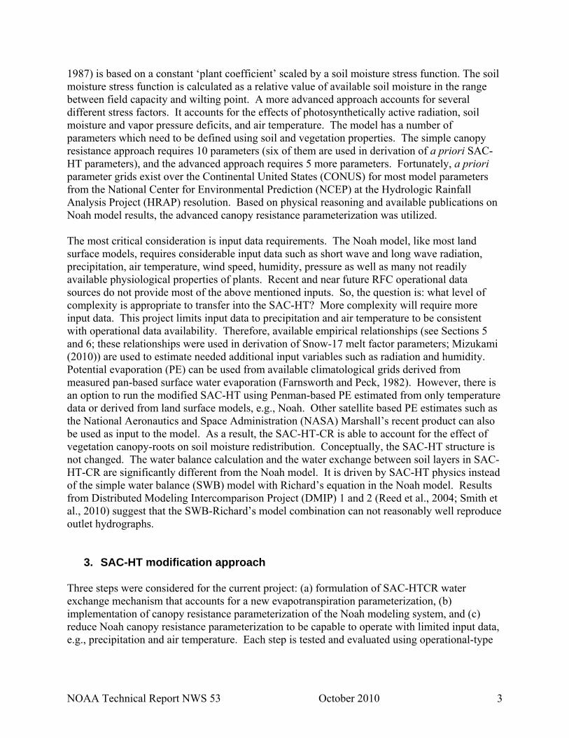
Soil moisture redistribution formulation. Because of significant differences in the formulation of evapotranspiration from SAC-HT and Noah, a water redistribution procedure is developed to incorporate the Noah definition into the SAC-HT environment. Fortunately, SAC-HT has the capability to recalculate its water storages into soil profile moisture contents (Fig. 3.1).
Figure 3.1. Schematic of moisture/heat states recalculation in SAC-HT
Similar to the SAC-HT definition, water redistribution is performed in two steps. First, SAC-HTCR states are adjusted for evapotranspiration mostly from tension water storages. The Noah
SAC-SMA storages SOIL layers SAC-SMA storages
SMC1
SMC2
SMC3
SMC4

NOAA Technical Report NWS 53 October 2010 7
Richards-based soil moisture exchange algorithm is used in this case instead of the SAC-HT direct water subtraction from each zone. However, layer- estimated evapotranspiration Ei is the only internal source in the equation:
, i = 1,2,…,n (3.14)
where i is the number of the soil layer.
Soil moisture contents at each layer estimated from this equation are then recalculated into SAC-HTCR upper and lower zone storages as shown in Fig. 3.2.
Figure 3.2. Schematic of water subtraction due to evapotranspiration
Elo=f(∆Ep,Slo)
Eup=f(Ep,Sup)
Ebare=f(Ep,σ,S1) Ecan=f(Ep,σ,Sc)
Etsp=f(Ep,σ,Si,Fr,Ft,Fq)
Etsp1
Etsp2
Etsp3
Etsp4
iiii EK
zDK
zD
t=+
∂∂
−+∂∂
+∂∂
−1)]()([)]()([ θθθθθθθ

NOAA Technical Report NWS 53 October 2010 8
This approach allows tension water exchange between upper and lower zones which the SAC-SMA and SAC-HT do not account for.
In the second step, adjustments are made to the storage water due to free water exchange and removal for different runoff components. SAC-HTCR utilizes the original SAC-SMA mechanism for free water exchange; the only difference is that at the end of each time step SAC-HTCR states are recalculated into soil profile moisture states.
This water redistribution scheme directly affected a number of SAC-HTCR components:
- Evapotranspiration rate (broken into bare soil and canopy transpiration)
- Evapotranspiration split between upper and lower zones
- Redistribution of soil moisture between upper and lower zones: Noah approach for tension water and SAC-HT for free water
- Removal of vegetation adjustment factors to the potential evaporation
3.2. Implementation of canopy resistance parameterization
The critical component in the estimation of evapotranspiration by Eq. (3.13) is the canopy resistance factor or plant coefficient Bc. Most land surface schemes including the Noah model employ a Jarvis-type or ‘meteorological’ (Niyogi and Raman, 1997) parameterization of the stomatal resistance. In these parameterizations, the stomatal resistance is modeled as a function of meteorological variables such as air temperature, vapor pressure, radiation, and soil moisture saturation (Jarvis, 1976; Noilhan and Planton, 1989; Chen and Dudhia, 2001). Alternatively, a ‘physiological’ approach is more common in climate change studies. This approach employs more rigorous plant gas-exchange responses such as carbon-assimilation rates, night respiration, and plant biochemical symptoms (Sellars et al., 1996; Niyogi and Raman, 1997). An important aspect of physiological models is that, though in theory they tend to mimic the physiological response, they are still empirical in nature and need not represent a casual relation. As stated by Niyogi and Raman (1997), some of these questions need to be addressed before practical implementation of physiological approaches in mesoscale models can occur.
The Noah model employs a Jarvis-type stomatal resistance parameterization. It actually uses the electric-circuit analogy to combine canopy and atmospheric resistances linked in series:
rch
rc RRC
RB
/1/1Δ++
Δ+= (3.15)
where Δ depends on the slope of the saturation specific humidity curve, Ch is the surface exchange coefficient for heat and moisture, Rr is a function of surface air temperature and pressure, and Rc is the total canopy resistance:

NOAA Technical Report NWS 53 October 2010 9
LAIFFFFR
RsmTqsr
cc ⋅⋅⋅⋅= min, (3.16)
The total canopy resistance Rc accounts for the: solar radiation effect
LAIRR
fwheref
fRRF
gl
gccsr
255.0_.......,1/ max,min, ⋅=+
+= (3.17)
vapor pressure effect
])([11
aassq qTqh
F−⋅+
= (3.18)
air temperature effect
2)(0016.01 arefT TTF −⋅−= (3.19) soil moisture effect
∑= ⋅−
⋅−=
nr
i nswf
iwism d
dF
1 )()(
θθθθ
(3.20)
where Rc,min and Rc,max are minimum and maximum [the cuticular resistance of the leaves from Dickinson et al. (1993)] stomatal resistance respectively, LAI is the leaf area index, Rgl is a solar radiation limit value, hs, Tref are empirical parameters, θd and θw are field capacity and wilting point respectively, di is the layer thickness, dnr is the total root zone thickness, and nr is the number of root zone layers, qa, qs , Ta, θi, and Rg are input variables water vapor mixing ratio, saturation mixing ratio, air temperature, soil moisture content, and solar radiation (the factor Fsr represents the influence of the photosynthetically active radiation, assumed to be 0.55 of the solar radiation), respectively.
NOAA Technical Report NWS 53 October 2010 10
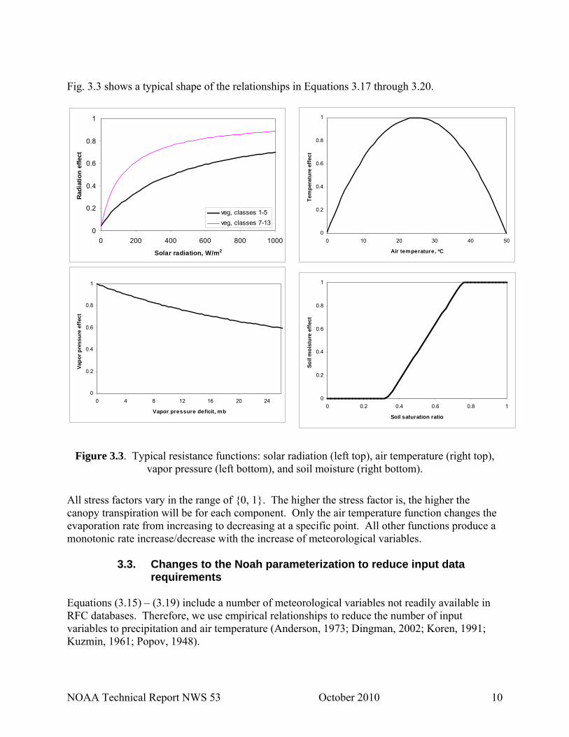
Fig. 3.3 shows a typical shape of the relationships in Equations 3.17 through 3.20.
0
0.2
0.4
0.6
0.8
1
0 10 20 30 40 50
Air temperature, oC
Tem
pera
ture
eff
ect
0
0.2
0.4
0.6
0.8
1
0 0.2 0.4 0.6 0.8 1
Soil saturation ratio
Soil
moi
stur
e ef
fect
Figure 3.3. Typical resistance functions: solar radiation (left top), air temperature (right top), vapor pressure (left bottom), and soil moisture (right bottom).
All stress factors vary in the range of {0, 1}. The higher the stress factor is, the higher the canopy transpiration will be for each component. Only the air temperature function changes the evaporation rate from increasing to decreasing at a specific point. All other functions produce a monotonic rate increase/decrease with the increase of meteorological variables.
3.3. Changes to the Noah parameterization to reduce input data requirements
Equations (3.15) – (3.19) include a number of meteorological variables not readily available in RFC databases. Therefore, we use empirical relationships to reduce the number of input variables to precipitation and air temperature (Anderson, 1973; Dingman, 2002; Koren, 1991; Kuzmin, 1961; Popov, 1948).
0
0.2
0.4
0.6
0.8
1
0 4 8 12 16 20 24
Vapor pressure deficit, mb
Vapo
r pre
ssur
e ef
fect
0
0.2
0.4
0.6
0.8
1
0 200 400 600 800 1000
Solar radiation, W/m2
Radi
atio
n ef
fect
veg, classes 1-5veg, classes 7-13

NOAA Technical Report NWS 53 October 2010 11
Solar radiation estimation. There are a number of semi-empirical relationships to estimate incoming short-wave solar radiation (Thompson, 1976; Bristow and Campbell, 1984; Hunt et al., 1998; Thornton and Running, 1999; Liu and Scott, 2001). Most of then are based on the use of air temperature data. For this project, we selected the Bristow and Campbell (1984) technique that is based on daily maximum and minimum air temperature. It actually estimates the daily atmospheric transmittance coefficient (Gates, 1980):
)]exp(1[/ Cdogt TBARRK ⋅−−⋅== (3.21)
where Rg is the actual daily solar radiation, Ro is the daily total extraterrestrial insulation incident on the horizontal surface, Td is the difference between daily maximum and minimum temperature, and A, B, C are empirical coefficients. Bristow and Campbell (1984) noted that although these coefficients are determined empirically, they do display the physics involved in the relationship. Coefficient A represents the maximum clear sky characteristics of the study area. It may vary with elevation and pollution content of the air. B and C determine how soon maximum Kt is achieved as Td is increases. They found that for tested data sets at different locations and elevations including Seattle/Tacoma, Washington coefficients A and C can be held constant at 0.7 and 2.4 respectively. Coefficient B values differ for winter and summer, 0.01 and 0.004, respectively. The extraterrestrial insulation on the horizontal surface incident can be estimated from astronomical relationships (Dingman, 2002):
]5.0)()()5.0()()([2 rsrsooo tSinlatSinrottrotSinCoslatCosESR ⋅⋅⋅+⋅⋅⋅⋅⋅⋅⋅⋅= δδ (3.22) where So = 117.54 cal/(cm2 hr) is the solar constant, Eo is the eccentricity correction, lat is latitude, δ is the sun declination, rot = 0.2618 radian/hr is the angular velocity of the earth’s rotation, and trs is the daylight time in hrs.
rotlattgtgarcCoslattgtgarcCostrs
)]()([)]()([ ⋅−−⋅−=
δδ (3.23)
Estimated daily radiation from (3.21) and (3.22) is converted into time interval instantaneous radiation values using sun angle at a specific time and the daylight time at a specific location. Water vapor pressure estimation. A simple relationship between water vapor pressure and air temperature (Popov, 1948) was used to estimate the water vapor canopy resistance factor e:
)0579.0exp(02.446 ate ⋅⋅= (3.24) Water vapor pressure is in Pa, and air temperature, ta, is in Celsius degrees. This relationship was derived using a number of stations located in different parts of the former USSR. The average error of equation (3.24) is less than 0.2 mm for daily average estimates and less than 0.3 mm for instantaneous estimates. For the use in the canopy resistance estimation, vapor pressure is converted into humidity or the vapor mixing ratio, q(Ta):

NOAA Technical Report NWS 53 October 2010 12
)622.01(
622.0)(eP
eTqa
a ⋅−−⋅
= (3.25)
where Pa is an air pressure in Pa, and the mixing ratio is in kg/kg. It is assumed that air pressure depends only on elevation but does not vary with time. Wind speed effect. Our goal is to reduce the required input data to precipitation and air temperature. However, the SAC-HTCR still uses wind speed in the estimation of the surface layer exchange coefficient. Simulation results suggest that wind effects on evapotranspiration are not as significant as on bare soil evaporation. One of the reasons is that the total effect of the wind -dependent surface layer exchange coefficient may be reduced by the Penman-Monteith equation. Therefore, it is possible to use a constant reference wind speed. However, SAC-HTCR can be run using different sources of potential evaporation which may not account directly for the variable wind speed, e.g., monthly climatological water surface evaporation (Ep). In this case, evapotranspiration estimation as a product of the potential evaporation and a plant coefficient (Bc) may be not consistent because climatological Pe does not account for wind speed but the Bc relationship (3.15) does account for wind speed. From Eq. (3.15) it follows that as wind speed approaches 0.0, Bc approaches 1.0. As wind speed approaches infinity, Bc approaches 0.0. It means that estimated evapotranspiration will decrease with wind speed increases. This behavior contradicts the basic theory. To overcome this problem, let us combine the Penman and plant coefficient equations to estimate actual evapotranspiration, Ea:
[ ]hchThT
hphnethTqpca CRCFCF
CFCRCFFEBE
⋅⋅++⋅Δ++
⋅⋅⋅Δ⋅++⋅=⋅=
)()1()(
(3.26)
where Fp and Fq are functions of air temperature, pressure, and humidity which are wind speed independent variables as well as net radiation, Rnetr. From (3.26) it follows that, as wind speed approaches 0.0, actual evapotranspiration approaches 0.0 and as wind speed approaches infinity, actual evapotranspiration approaches a maximum value Ea,max:
cT
netqpa RF
RFFE
⋅+
Δ⋅+⋅⋅=
)1()(2
max, (3.27)
Evapotranspiration in this case is driven by atmospheric conditions and canopy resistance, and it is not restricted by the surface air exchange. To preserve these properties, wind independent potential evaporation input data were multiplied by a ratio of Penman potential evaporation estimated with the use of actual wind speed, Epen,act, and reference wind speed, Epen,ref:
refpen
actpenpadjp E
EEE
,
,, ⋅= (3.28)

NOAA Technical Report NWS 53 October 2010 13
Penman evaporation was estimated using the Noah algorithm but radiation and air humidity were calculated from empirical relationships (3.21), (3.22), and (3.24). We recognize that the reference wind speed may vary in space. However, a constant reference wind speed of 3.0 m/s is used in most tests for the Oklahoma Mesonet region. Solar radiation estimation tests. To check the validity of the Bristow and Campbell (1984) approach and specifically the relationship parameters, simulations were performed using solar radiation measurements from SnowMIP2 (Essery et al., 2009) and the Oklahoma Mesonet. Fig. 3.4 is a scatter plot of estimated and observed short wave radiation at three SnowMIP2 sites and one Oklahoma Mesonet site. Overall, a reasonable relationship is achieved even at half hourly time intervals with correlation coefficient in the range from 0.77 to 0.82 for different sites. These simulations were performed using a value of 0.75 for parameter A which provided somewhat better results compared to the original value A = 0.7.
Figure 3.4. Comparison of observed and estimated half hourly radiation for SnowMIP2 (left panel) and hourly radiation for Oklahoma Mesonet site (right panel).
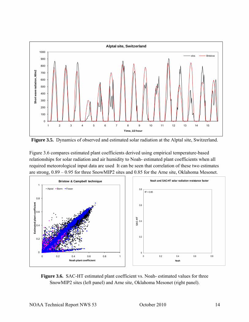
Dynamics of half hourly radiation at the SnowMIP2 Alptal site are shown in Fig. 3.5. Good agreement between observed and simulated diurnal variability of solar radiation can be seen in the figure.
0
200
400
600
800
1000
1200
0 200 400 600 800 1000 1200
Estim
ated
sol
ar ra
diat
ion
Observed solar radiation
Bristow & Campbell technique
Alptal Berm Fraser
Observed and estimated solar radiation at ARNE site, W/m2
0
200
400
600
800
1000
1200
0 200 400 600 800 1000 1200
Observed
Estim
ated
R2 = 0.82
NOAA Technical Report NWS 53 October 2010 14
Figure 3.5. Dynamics of observed and estimated solar radiation at the Alptal site, Switzerland.
Figure 3.6 compares estimated plant coefficients derived using empirical temperature-based relationships for solar radiation and air humidity to Noah- estimated plant coefficients when all required meteorological input data are used It can be seen that correlation of these two estimates are strong, 0.89 – 0.95 for three SnowMIP2 sites and 0.85 for the Arne site, Oklahoma Mesonet.
Figure 3.6. SAC-HT estimated plant coefficient vs. Noah- estimated values for three
SnowMIP2 sites (left panel) and Arne site, Oklahoma Mesonet (right panel).
0
100
200
300
400
500
600
700
800
900
1000
1 2 3 4 5 6 7 8 9 10 11 12 13 14 15
Shor
t wav
e ra
diat
ion,
W/m
2
Time, 1/2 hour
Alptal site, Switzerland
obs Bristow
0
0.2
0.4
0.6
0.8
1
0 0.2 0.4 0.6 0.8 1
Estim
ated
pla
nt c
oeff
icie
nt
Noah plant coefficient
Bristow & Campbell technique
Alptal Berm Fraser
Noah and SAC-HT solar radiation resistance factor
0
0.2
0.4
0.6
0.8
0 0.2 0.4 0.6 0.8
Noah
SAC
-HT
R2 = 0.85

NOAA Technical Report NWS 53 October 2010 15
3.4. Parametric data The modified SAC-HTCR uses the same basic parameters as the original SAC-HT. However, 12 monthly vegetation adjustment factors to potential evaporation are eliminated because of explicit use of the canopy-based evapotranspiration mechanism. These 12 values typically need to be calibrated. The Noah evapotranspiration parameterization introduces a new set of parameters. There are two types of land-surface parameters: a) single universal values, b) values dependent on the vegetation class index. a) Single universal values include: - CZIL = 0.12: Zilitinkevich parameter (range 0.0-1.0) which controls the ratio of the roughness length for heat to the roughness length for momentum. This parameter allows tuning of the aerodynamic resistance of the atmospheric surface layer. Increasing CZIL increases aerodynamic resistance and, as a result, reduces evapotranspiration, - χ = 2.0: bare soil evaporation exponent in non-linear parameterization, - n = 0.5: the exponent in the function for canopy surface water evaporation, - Wmc = 0.0005 m: maximum canopy water capacity used in canopy water evaporation, - Rc,max = 5000 s/m: maximum stomatal resistance, - Tref = 298 K: optimum air temperature for transpiration. b) Parameters dependent on the vegetation class index. NCEP used the University of Maryland (UM) vegetation classes:
1: Evergreen Needleleaf Forest 2: Evergreen Broadleaf Forest 3: Deciduous Needleleaf Forest 4: Deciduous Broadleaf Forest 5: Mixed Forest 6: Woodland 7: Wooded Grassland 8: Closed Shrubland 9: Open Shrubland 10: Grassland 11: Cropland 12: Bare Ground 13: Urban and Built-up 14: Water
They generated CONUS grids of most of the vegetation-dependent parameters:
- Rc,min is minimal stomatal resistance, s/m, - Rgl is solar radiation threshold for which resistance factor Rsr is about to double its
minimum value, - hs is a parameter in the vapor pressure resistance factor,
NOAA Technical Report NWS 53 October 2010 16
- Zo is the roughness length, m, - Nrt is the number of soil layers with roots - LAI is the leaf area index presently set to universal value of 5.0.
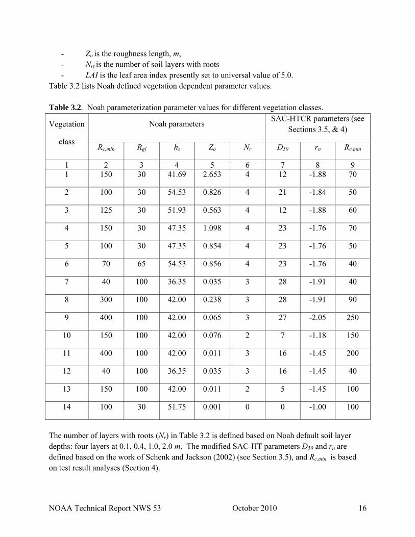
Table 3.2 lists Noah defined vegetation dependent parameter values. Table 3.2. Noah parameterization parameter values for different vegetation classes.
Vegetation
class
Noah parameters SAC-HTCR parameters (see
Sections 3.5, & 4)
Rc,min Rgl hs Zo Nr D50 rn Rc,min
1 2 3 4 5 6 7 8 91 150 30 41.69 2.653 4 12 -1.88 70
2 100 30 54.53 0.826 4 21 -1.84 50
3 125 30 51.93 0.563 4 12 -1.88 60
4 150 30 47.35 1.098 4 23 -1.76 70
5 100 30 47.35 0.854 4 23 -1.76 50
6 70 65 54.53 0.856 4 23 -1.76 40
7 40 100 36.35 0.035 3 28 -1.91 40
8 300 100 42.00 0.238 3 28 -1.91 90
9 400 100 42.00 0.065 3 27 -2.05 250
10 150 100 42.00 0.076 2 7 -1.18 150
11 400 100 42.00 0.011 3 16 -1.45 200
12 40 100 36.35 0.035 3 16 -1.45 40
13 150 100 42.00 0.011 2 5 -1.45 100
14 100 30 51.75 0.001 0 0 -1.00 100
The number of layers with roots (Nr) in Table 3.2 is defined based on Noah default soil layer depths: four layers at 0.1, 0.4, 1.0, 2.0 m. The modified SAC-HT parameters D50 and rn are defined based on the work of Schenk and Jackson (2002) (see Section 3.5), and Rc,min is based on test result analyses (Section 4).
NOAA Technical Report NWS 53 October 2010 17
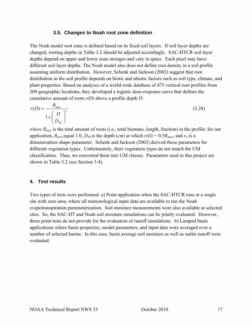
3.5. Changes to Noah root zone definition The Noah model root zone is defined based on its fixed soil layers. If soil layer depths are changed, rooting depths in Table 3.2 should be adjusted accordingly. SAC-HTCR soil layer depths depend on upper and lower zone storages and vary in space. Each pixel may have different soil layer depths. The Noah model also does not define root density in a soil profile assuming uniform distribution. However, Schenk and Jackson (2002) suggest that root distribution in the soil profile depends on biotic and abiotic factors such as soil type, climate, and plant properties. Based on analyses of a world-wide database of 475 vertical root profiles from 209 geographic locations, they developed a logistic dose-response curve that defines the cumulative amount of roots r(D) above a profile depth D:
nr
DD
RDr
⎟⎟⎠
⎞⎜⎜⎝
⎛+
=
50
max
1
)( (3.28)
where Rmax is the total amount of roots (i.e., total biomass, length, fraction) in the profile; for our application, Rmax equal 1.0, D50 is the depth (cm) at which r(D) = 0.5Rmax, and rn is a dimensionless shape-parameter. Schenk and Jackson (2002) derived these parameters for different vegetation types. Unfortunately, their vegetation types do not match the UM classification. Thus, we converted them into UM classes. Parameters used in this project are shown in Table 3.2 (see Section 3.4). 4. Test results Two types of tests were performed: a) Point application when the SAC-HTCR runs at a single site with zero area, where all meteorological input data are available to run the Noah evapotranspiration parameterization. Soil moisture measurements were also available at selected sites. So, the SAC-HT and Noah soil moisture simulations can be jointly evaluated. However, these point tests do not provide for the evaluation of runoff simulations. b) Lumped basin applications where basin properties, model parameters, and input data were averaged over a number of selected basins. In this case, basin average soil moisture as well as outlet runoff were evaluated.

NOAA Technical Report NWS 53 October 2010 18
4.1. Point-type application
Five Oklahoma Mesonet sites with a wide range of a climate index (mean annual greenness fraction was used as an index) were selected for the tests, see Table 4.1. Table 4.1. Tested Oklahoma Mesonet sites
Site ID Latitude Longitude Elevation, m Climate Index
BOIS 36.69 -102.50 1267 0.24
ARNE 36.07 -99.90 719 0.31
ACME 34.80 -98.02 397 0.42
LANE 34.31 -96.00 181 0.51
WEST 36.01 -94.64 348 0.60
At an early stage in the project, soil measurements and input data were also collected from the Hydrometeorology Testbed (HMT; Zamora et al., 2009) observations in the Arizona region. However, the data were available for only about one year. Because of very long memory of soil moisture states in this type arid zone, it was impossible to generate reasonable initial model states. Therefore these data were not used in model evaluation. All Oklahoma sites are located in the North American Prairies region with vegetation type ranging from tall grass prairie that reaches a height of 6 feet and a root depth up to 9 feet, to short grass prairie that reaches a height of 48 inches and a root depth up to 5 feet. However, the Noah parametric data defines only one grassland category. To account for differences in site vegetation properties, the root depth for each site was defined manually using site description information. Our test approach included the following: - A priori SAC-HT parameters; no calibration
- Noah-defined vegetation related parameters excluding root depth/distribution - Observed precipitation, air temperature, and wind speed data at each site are used for SAC-HT; in addition, short wave solar radiation, air pressure, and relative humidity are used for the Noah model. - Monthly climatological potential evaporation, PE, (water surface evaporation) is used for SAC-HT and Penman-based PE in Noah simulations. - No vegetation adjustment to PE values for SAC-HTCR; however, monthly vegetation adjustment to PE is used for the original SAC-HT.

NOAA Technical Report NWS 53 October 2010 19
Hourly data for selected sites were provided by Oklahoma Mesonet personnel for the period 1996 – 2002. Precipitation, air temperature, solar radiation, relative humidity, wind speed, and air pressure data were provided. Soil moisture observations at 5 cm as well as the average of the upper (0-25 cm) and lower (25-75 cm) soil layers were available from previous studies (Koren et al., 2006). Figure 4.1 displays simulations (2-year period of 7 years is selected) from the original SAC-HT, modified SAC-HTCR, and Noah for a dry Mesonet site (ARNE; climate index 0.31). Soil moisture at 5 cm, and upper and lower soil layers are compared to measured daily values. Upper and lower zone SAC-HT storage dynamics are also plotted. Overall, the modified SAC-HTCR better reproduces soil moisture measurements at all soil layers, especially the lower layer. Underestimation of soil moisture at lower layers compared to the original model is reduced significantly for this dry site. This underprediction was the main reason for the evapotranspiration component modification. Soil moisture changes led to significant changes in the SAC-HT storages. Lower zone storage contents increased about two times compared to the old version. The Noah model tends to overestimate soil moisture at all soil layers (note that Noah potential evaporation estimates were used for Noah simulations). It shows much variability at the 5 cm layer and soil moisture often drops down to the lower limit. One of the causes may be numerical solution instability because of the 1-hr computational time step.

NOAA Technical Report NWS 53 October 2010 20
Figure 4.1. Observed (red) and Simulated Soil Moisture at 5cm (4), 0-25 (5), 25-75 (6), and Upper (2) & Lower (3) SAC Storages: ARNE site (Climate Index = 0.31). Lines: white –
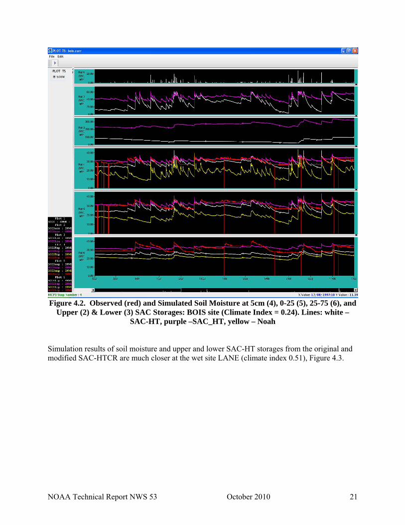
SAC-HT, purple –SAC-HTCR, yellow - Noah Figure 4.2 is a similar plot for the driest Mesonet site (BOIS; climate index 0.24). The biggest difference is in underestimation of soil moisture by Noah model at all layers compared to overestimation at ARNE site. The original SAC-HT soil moisture at upper layers is closer to modified version and measurement, however, the lower layer soil moisture is still underestimated. Simulation results of soil moisture and upper and lower SAC-HT storages from the original and modified SAC-HTCR are much closer at the wet site LANE (climate index 0.51), Figure 4.3.
NOAA Technical Report NWS 53 October 2010 21
Figure 4.2. Observed (red) and Simulated Soil Moisture at 5cm (4), 0-25 (5), 25-75 (6), and Upper (2) & Lower (3) SAC Storages: BOIS site (Climate Index = 0.24). Lines: white –
SAC-HT, purple –SAC_HT, yellow – Noah Simulation results of soil moisture and upper and lower SAC-HT storages from the original and modified SAC-HTCR are much closer at the wet site LANE (climate index 0.51), Figure 4.3.

NOAA Technical Report NWS 53 October 2010 22
Figure 4.3. Observed (yellow) and Simulated Soil Moisture at 5cm (4), 0-25 (5), 25-75 (6),
and Upper (2) & Lower (3) SAC Storages: LANE site (Climate Index = 0.51). Lines: white – SAC-HT, purple –SAC-HTCR
Tables 4.2 and 4.3 present overall statistics for the lower and upper soil layers. All lower layer statistics from the original SAC-HT are consistently worse compared to the modified version, having a systematic negative bias. The biggest bias and RMSE occur at dryer sites. Upper layer statistics are less consistent. While bias and RMSE values from the modified version are consistently better than the original version, correlation is slightly worse. It should be noted that there are significant uncertainties in soil moisture measurements at the hourly time step. A comparison of monthly climatological soil moisture at three layers estimated as 6-year averages is shown in Figures 4.4 and 4.5. Some explanation of the correlation reduction in modified version at upper soil layers for dry sites can be drawn from Figure 4.4. It can be seen that modified version soil moisture dynamics are less sensitive to the seasonal variability seen in original version and measurements. The most probable cause is evapotranspiration variability with season. Analysis of evapotranspiration season dependency and its improvement will be discussed in the next section.

NOAA Technical Report NWS 53 October 2010 23
Table 4.2. Hourly soil moisture statistics from original and modified SAC-HT at the lower layer
Site ID Gind SAC-HTCR SAC-HT
%Bias %RMSE R %Bias %RMSE R BOIS 0.245 9.6 14.2 0.50 -14.9 18.2 0.43 ARNE 0.306 -8.6 11.3 0.80 -23.4 25.8 0.84 ACME 0.425 4.6 11.3 0.85 -19.4 26.7 0.72 LINE 0.510 -4.1 8.9 0.89 -9.7 17.2 0.81 WEST 0.600 4.4 11.3 0.78 1.3 10.4 0.79 Avg 0.417 1.2 11.4 0.76 -13.2 19.7 0.72 Table 4.3. Hourly soil moisture statistics from original and modified SAC-HT at the upper layer
Site ID Gind SAC-HTCR SAC-HT
%Bias %RMSE R %Bias %RMSE R BOIS 0.245 -6.0 11.0 0.60 7.3 11.2 0.72 ARNE 0.306 14.8 17.4 0.80 19.1 22.2 0.87 ACME 0.425 9.2 13.3 0.72 22.0 25.3 0.83 LINE 0.510 8.4 11.8 0.85 18.1 22.9 0.77 WEST 0.600 9.4 14.3 0.77 15.5 17.6 0.88 Avg 0.417 7.2 13.6 0.75 16.4 19.8 0.81 All simulations with the modified SAC-HTCR version were performed using a non-linear bare soil evaporation approach that usually evaporates less than a linear approach under the same meteorological conditions. Figure 4.6 compares results from non-linear and linear versions. The non-linear version results agree better with measurements at all soil layers. The linear version subtracts more water for evaporation and as a result underestimates soil moisture consistently at all layers. Soil moisture estimates from the two versions are much closer during the vegetation growing season when the impact of bare soil evaporation is reduced. Figure 4.6 also presents results from the non-linear version when the original SAC-HT soil moisture redistribution is used instead of the mixed redistribution mechanism developed for modified version. It can be seen that the use of the original model mechanism leads to a significant inconsistency in soil moisture estimation: at 5 cm top layer moisture is too low, at 0-25 cm it is reasonable, and at 25-75 cm it is too high. Therefore, later on in the lumped basin simulations a mixed SAC-HTCR mechanism is used. The evapotranspiration rate is very sensitive to the minimal stomatal resistance parameter, Rc,min. For example, Jacquemin and Noilhan (1990) found that changing the Rc,min parameter by 10% can change latent heat flux (evaporation) by about 80%. Of course, such big changes in evapotranspiration can occur under wet soil conditions. Our simulations suggest similar behavior. Figure 4.7 compares results from a modified SAC-HT for Rc,min = 50 s/m and Rc,min = 150 s/m. Soil moisture is much higher in the second case specifically during vegetation growing season. These results suggest that selection of the minimal stomatal resistance parameter is critical and may require some tuning to achieve reasonable simulation result. More analysis on this parameter will be presented in the next section.

NOAA Technical Report NWS 53 October 2010 24
Figure 4.4. Soil moisture monthly climatology from SAC-HT and modified SAC-HTCR vs. measurements at ARNE site
6-year average monthly soil moisture at 5 cm: ARNE, G=0.306
0.1
0.15
0.2
0.25
0.3
1 2 3 4 5 6 7 8 9 10 11 12
Month
Volum
etric
soil m
oist
ure
sac modsac obs
6-year average monthly soil moisture at 0-25 cm: ARNE, G=0.306
0.1
0.15
0.2
0.25
0.3
1 2 3 4 5 6 7 8 9 10 11 12
Month
Volum
etric
soil m
oist
ure
sac modsac obs
6-year average monthly soil moisture at 25-75 cm: ARNE, G=0.306
0.1
0.15
0.2
0.25
0.3
1 2 3 4 5 6 7 8 9 10 11 12
Month
Volum
etric
soil m
oist
ure
sac modsac obs

NOAA Technical Report NWS 53 October 2010 25
Figure 4.5. Soil moisture monthly climatology from SAC-HT and modified SAC-HTCR vs. measurements at LANE site
6-year average monthly soil moisture at 5 cm: LANE, G=0.510
0.1
0.15
0.2
0.25
0.3
0.35
1 2 3 4 5 6 7 8 9 10 11 12
Month
Volum
etric
soil m
oist
ure
sac modsac obs
6-year average monthly soil moisture at 0-25 cm: LANE, G=0.510
0.1
0.15
0.2
0.25
0.3
0.35
1 2 3 4 5 6 7 8 9 10 11 12
Month
Volu
met
ric soil m
oist
ure
sac modsac obs
6-year average monthly soil moisture at 25-75 cm: LANE, G=0.510
0.1
0.15
0.2
0.25
0.3
0.35
1 2 3 4 5 6 7 8 9 10 11 12
Month
Volu
met
ric soil m
oist
ure
sac modsac obs

NOAA Technical Report NWS 53 October 2010 26
Figure 4.6. Effect of linear and non-linear options of bare soil evaporation on soil moisture at 5cm (4), 0-25 (5), 25-75 (6), and upper (2) & lower (3) SAC storages: ARNE site (Climate Index = 0.306). Lines: red – Observed, white – Non-linear, purple – Linear, yellow – Non-
linear with SAC redistribution

NOAA Technical Report NWS 53 October 2010 27
Figure 4.7. Effect of Rc,min resistance parameter on soil moisture at 5cm (4), 0-25 (5),
25-75 (6), and upper (2) & lower (3) SAC storages: LANE site (Climate Index = 0.51). Lines: yellow – Observed, white – Rsmin=40, purple – Rsmin=150
4.2. Lumped basins application
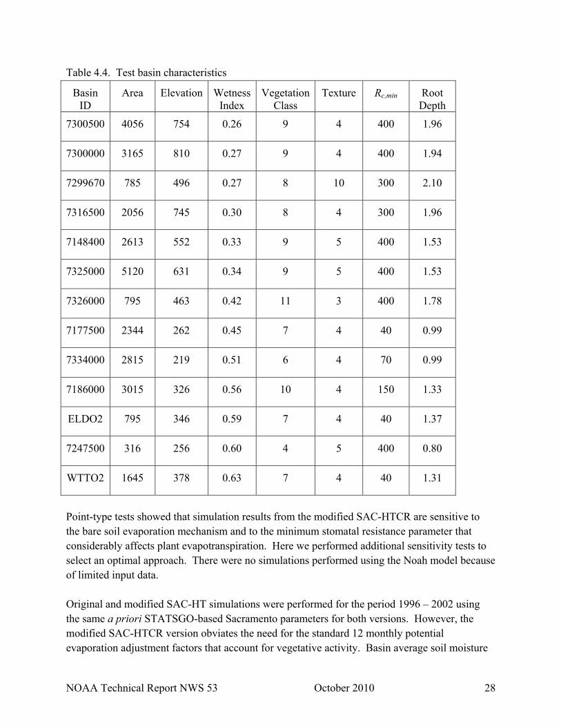
Thirteen river basins were selected in the Oklahoma Mesonet region to cover as many as possible land cover classes and values of basin wetness index, Gind. Unfortunately, meteorological data were available only at a few sites used in the point-type tests. Therefore, only precipitation from NEXRAD grids and air temperature from the North American Regional Reanalysis (NARR; Meisinger et al., 2006) were used in these simulations. Because the recent version of HL-RDHM software was not modified to define the new introduced parametric grids, vegetation and soil texture related properties were estimated from basin average vegetation and soil classes. This can lead to some inconsistency in the average basin properties. Table 4.4 presents the main basin characteristics as they are defined in the Noah database.
NOAA Technical Report NWS 53 October 2010 28
Table 4.4. Test basin characteristics
Basin ID
Area Elevation Wetness Index
Vegetation Class
Texture Rc,min Root Depth
7300500 4056 754 0.26 9 4 400 1.96
7300000 3165 810 0.27 9 4 400 1.94
7299670 785 496 0.27 8 10 300 2.10
7316500 2056 745 0.30 8 4 300 1.96
7148400 2613 552 0.33 9 5 400 1.53
7325000 5120 631 0.34 9 5 400 1.53
7326000 795 463 0.42 11 3 400 1.78
7177500 2344 262 0.45 7 4 40 0.99
7334000 2815 219 0.51 6 4 70 0.99
7186000 3015 326 0.56 10 4 150 1.33
ELDO2 795 346 0.59 7 4 40 1.37
7247500 316 256 0.60 4 5 400 0.80
WTTO2 1645 378 0.63 7 4 40 1.31
Point-type tests showed that simulation results from the modified SAC-HTCR are sensitive to the bare soil evaporation mechanism and to the minimum stomatal resistance parameter that considerably affects plant evapotranspiration. Here we performed additional sensitivity tests to select an optimal approach. There were no simulations performed using the Noah model because of limited input data. Original and modified SAC-HT simulations were performed for the period 1996 – 2002 using the same a priori STATSGO-based Sacramento parameters for both versions. However, the modified SAC-HTCR version obviates the need for the standard 12 monthly potential evaporation adjustment factors that account for vegetative activity. Basin average soil moisture
NOAA Technical Report NWS 53 October 2010 29
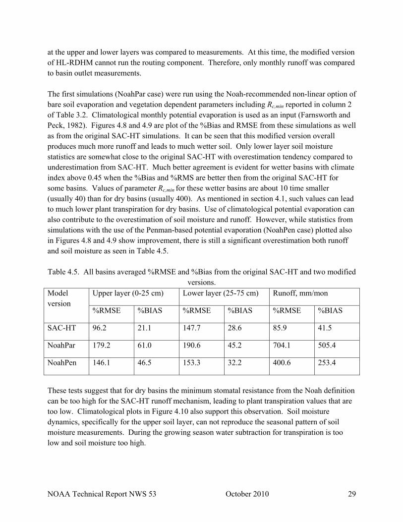
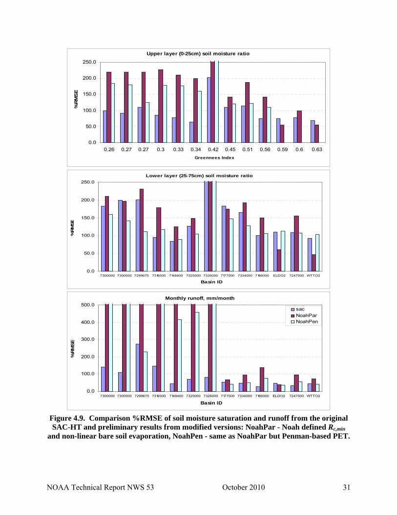
at the upper and lower layers was compared to measurements. At this time, the modified version of HL-RDHM cannot run the routing component. Therefore, only monthly runoff was compared to basin outlet measurements. The first simulations (NoahPar case) were run using the Noah-recommended non-linear option of bare soil evaporation and vegetation dependent parameters including Rc,min reported in column 2 of Table 3.2. Climatological monthly potential evaporation is used as an input (Farnsworth and Peck, 1982). Figures 4.8 and 4.9 are plot of the %Bias and RMSE from these simulations as well as from the original SAC-HT simulations. It can be seen that this modified version overall produces much more runoff and leads to much wetter soil. Only lower layer soil moisture statistics are somewhat close to the original SAC-HT with overestimation tendency compared to underestimation from SAC-HT. Much better agreement is evident for wetter basins with climate index above 0.45 when the %Bias and %RMS are better then from the original SAC-HT for some basins. Values of parameter Rc,min for these wetter basins are about 10 time smaller (usually 40) than for dry basins (usually 400). As mentioned in section 4.1, such values can lead to much lower plant transpiration for dry basins. Use of climatological potential evaporation can also contribute to the overestimation of soil moisture and runoff. However, while statistics from simulations with the use of the Penman-based potential evaporation (NoahPen case) plotted also in Figures 4.8 and 4.9 show improvement, there is still a significant overestimation both runoff and soil moisture as seen in Table 4.5. Table 4.5. All basins averaged %RMSE and %Bias from the original SAC-HT and two modified
versions. Model version
Upper layer (0-25 cm) Lower layer (25-75 cm) Runoff, mm/mon
%RMSE %BIAS %RMSE %BIAS %RMSE %BIAS
SAC-HT 96.2 21.1 147.7 28.6 85.9 41.5
NoahPar 179.2 61.0 190.6 45.2 704.1 505.4
NoahPen 146.1 46.5 153.3 32.2 400.6 253.4
These tests suggest that for dry basins the minimum stomatal resistance from the Noah definition can be too high for the SAC-HT runoff mechanism, leading to plant transpiration values that are too low. Climatological plots in Figure 4.10 also support this observation. Soil moisture dynamics, specifically for the upper soil layer, can not reproduce the seasonal pattern of soil moisture measurements. During the growing season water subtraction for transpiration is too low and soil moisture too high.

NOAA Technical Report NWS 53 October 2010 30
Upper layer (0-25cm) soil moisture ratio
-30.0
0.0
30.0
60.0
90.0
120.0
0.26 0.27 0.27 0.3 0.33 0.34 0.42 0.45 0.51 0.56 0.59 0.6 0.63
Greennees Index
%Bi
as
Lower layer (25-75cm) soil moisture ratio
-50.0
-25.0
0.0
25.0
50.0
75.0
7300000 7300500 7299670 7316500 7148400 7325000 7326000 7177500 7334000 7186000 ELDO2 7247500 WTTO2
Basin ID
%Bi
as
Monthly runoff, mm/month
-100.0
0.0
100.0
200.0
300.0
400.0
500.0
7300000 7300500 7299670 7316500 7148400 7325000 7326000 7177500 7334000 7186000 ELDO2 7247500 WTTO2
Basin ID
%Bi
as
sacNoahParNoahPen
Figure 4.8. Comparison of %RMSE of soil moisture saturation and runoff from the
original SAC-HT and preliminary results from modified versions: NoahPar - Noah defined Rc,min and non-linear bare soil evaporation, NoahPen - same as NoahPar but Penman-based
PET.
NOAA Technical Report NWS 53 October 2010 31
Upper layer (0-25cm) soil moisture ratio
0.0
50.0
100.0
150.0
200.0
250.0
0.26 0.27 0.27 0.3 0.33 0.34 0.42 0.45 0.51 0.56 0.59 0.6 0.63Greennees Index
%RM
SE
Lower layer (25-75cm) soil moisture ratio
0.0
50.0
100.0
150.0
200.0
250.0
7300000 7300500 7299670 7316500 7148400 7325000 7326000 7177500 7334000 7186000 ELDO2 7247500 WTTO2
Basin ID
%RM
SE
Monthly runoff, mm/month
0.0
100.0
200.0
300.0
400.0
500.0
7300000 7300500 7299670 7316500 7148400 7325000 7326000 7177500 7334000 7186000 ELDO2 7247500 WTTO2
Basin ID
%RM
SE
sacNoahParNoahPen
Figure 4.9. Comparison %RMSE of soil moisture saturation and runoff from the original SAC-HT and preliminary results from modified versions: NoahPar - Noah defined Rc,min
and non-linear bare soil evaporation, NoahPen - same as NoahPar but Penman-based PET.

NOAA Technical Report NWS 53 October 2010 32
Basin 7300000, G=0.26
0
0.1
0.2
0.3
0.4
0.5
0.6
1 2 3 4 5 6 7 8 9 10 11 12
Month
Upp
er L
ayer
SM
sat
urat
ion
obssacNoahPar
Basin 7300000, G=0.26
0
0.1
0.2
0.3
0.4
0.5
0.6
0.7
1 2 3 4 5 6 7 8 9 10 11 12
Month
Low
er la
yer S
M s
atur
atio
n
obssacNoahPar
Basin 7300000, G=0.26
0
5
10
15
20
25
30
1 2 3 4 5 6 7 8 9 10 11 12
Month
Mon
thly
runo
ff, m
m/m
onth
obssacNoahPar
Figure 4.10. Soil moisture and runoff monthly climatology from the original SAC-HT and
preliminary results from modified version NoahPar, Noah defined Rc,min and non-linear bare soil evaporation, vs. measurements for basin #7300000.
NOAA Technical Report NWS 53 October 2010 33
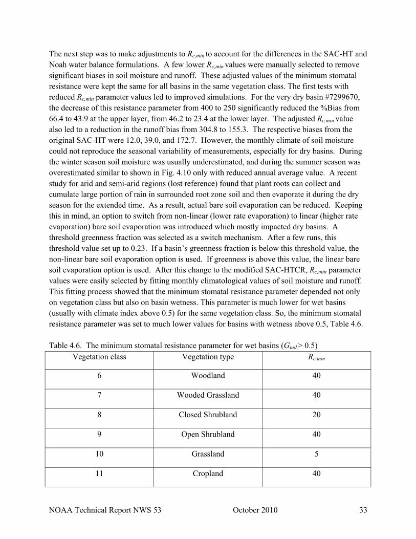
The next step was to make adjustments to Rc,min to account for the differences in the SAC-HT and Noah water balance formulations. A few lower Rc,min values were manually selected to remove significant biases in soil moisture and runoff. These adjusted values of the minimum stomatal resistance were kept the same for all basins in the same vegetation class. The first tests with reduced Rc,min parameter values led to improved simulations. For the very dry basin #7299670, the decrease of this resistance parameter from 400 to 250 significantly reduced the %Bias from 66.4 to 43.9 at the upper layer, from 46.2 to 23.4 at the lower layer. The adjusted Rc,min value also led to a reduction in the runoff bias from 304.8 to 155.3. The respective biases from the original SAC-HT were 12.0, 39.0, and 172.7. However, the monthly climate of soil moisture could not reproduce the seasonal variability of measurements, especially for dry basins. During the winter season soil moisture was usually underestimated, and during the summer season was overestimated similar to shown in Fig. 4.10 only with reduced annual average value. A recent study for arid and semi-arid regions (lost reference) found that plant roots can collect and cumulate large portion of rain in surrounded root zone soil and then evaporate it during the dry season for the extended time. As a result, actual bare soil evaporation can be reduced. Keeping this in mind, an option to switch from non-linear (lower rate evaporation) to linear (higher rate evaporation) bare soil evaporation was introduced which mostly impacted dry basins. A threshold greenness fraction was selected as a switch mechanism. After a few runs, this threshold value set up to 0.23. If a basin’s greenness fraction is below this threshold value, the non-linear bare soil evaporation option is used. If greenness is above this value, the linear bare soil evaporation option is used. After this change to the modified SAC-HTCR, Rc,min parameter values were easily selected by fitting monthly climatological values of soil moisture and runoff. This fitting process showed that the minimum stomatal resistance parameter depended not only on vegetation class but also on basin wetness. This parameter is much lower for wet basins (usually with climate index above 0.5) for the same vegetation class. So, the minimum stomatal resistance parameter was set to much lower values for basins with wetness above 0.5, Table 4.6. Table 4.6. The minimum stomatal resistance parameter for wet basins (Gind > 0.5)
Vegetation class Vegetation type Rc,min
6 Woodland 40
7 Wooded Grassland 40
8 Closed Shrubland 20
9 Open Shrubland 40
10 Grassland 5
11 Cropland 40

NOAA Technical Report NWS 53 October 2010 34
Figures 4.11 and 4.12 compare different statistics from the original and final modified SAC-HTCR.
Upper layer (0-25cm) soil moisture ratio
-20.0
0.0
20.0
40.0
60.0
80.0
0.26 0.27 0.27 0.3 0.33 0.34 0.42 0.45 0.51 0.56 0.59 0.6 0.63
Greennees Index
%Bi
as
Lower layer (25-75cm) soil moisture ratio
-60.0
-40.0
-20.0
0.0
20.0
40.0
60.0
80.0
7300000 7300500 7299670 7316500 7148400 7325000 7326000 7177500 7334000 7186000 ELDO2 7247500 WTTO2
Basin ID
%Bi
as
Monthly runoff, mm/month
-80.0
-40.0
0.0
40.0
80.0
120.0
160.0
7300000 7300500 7299670 7316500 7148400 7325000 7326000 7177500 7334000 7186000 ELDO2 7247500 WTTO2
Basin ID
%Bi
as
sacmodsac
Figure 4.11. Comparison of %Bias of soil moisture saturation and monthly runoff
from the original and modified SAC-HT.

NOAA Technical Report NWS 53 October 2010 35
Upper layer (0-25cm) soil moisture ratio
0.0
50.0
100.0
150.0
200.0
0.26 0.27 0.27 0.3 0.33 0.34 0.42 0.45 0.51 0.56 0.59 0.6 0.63
Greennees Index
%RM
SE
Lower layer (25-75cm) soil moisture ratio
0.0
50.0
100.0
150.0
200.0
7300000 7300500 7299670 7316500 7148400 7325000 7326000 7177500 7334000 7186000 ELDO2 7247500 WTTO2
Basin ID
%RM
SE
Monthly runoff, mm/month
0.0
50.0
100.0
150.0
200.0
7300000 7300500 7299670 7316500 7148400 7325000 7326000 7177500 7334000 7186000 ELDO2 7247500 WTTO2
Basin ID
%RM
SE
sacmodsac
Figure 4.12. Comparison of %RMSE of soil moisture saturation and monthly runoff
from the original and modified SAC-HT.
NOAA Technical Report NWS 53 October 2010 36
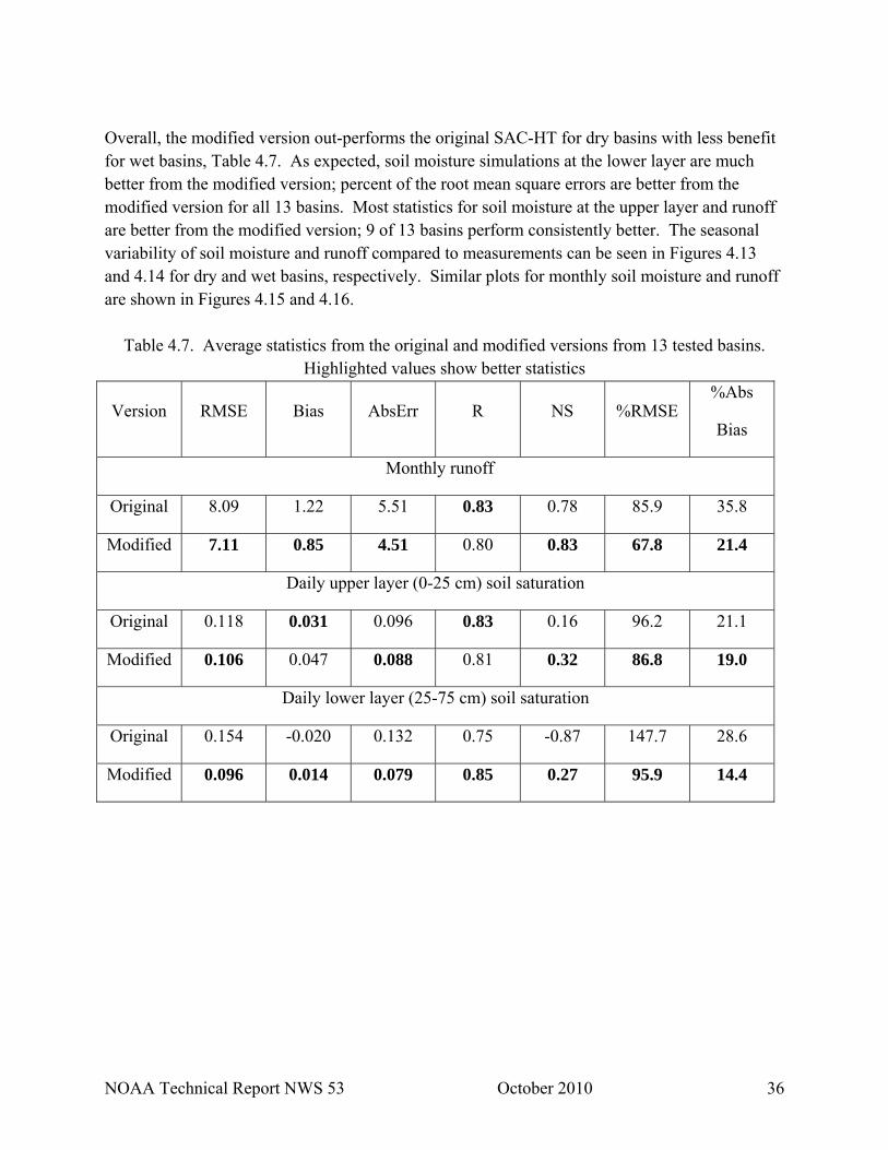
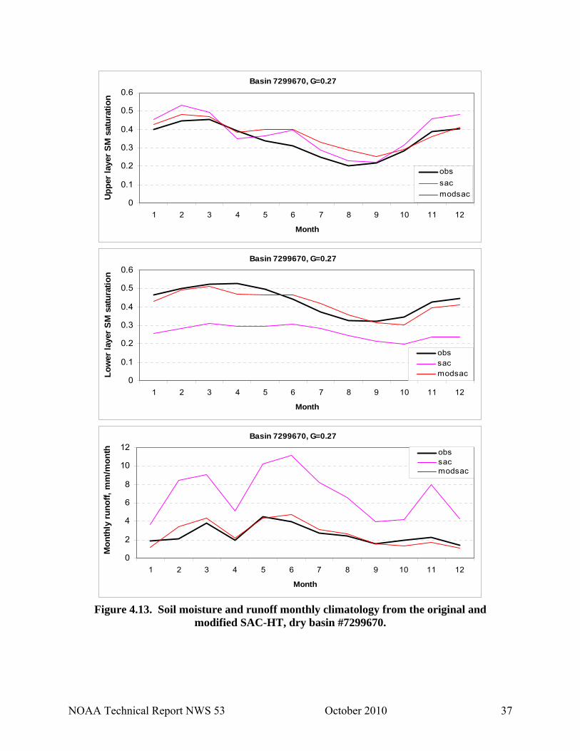
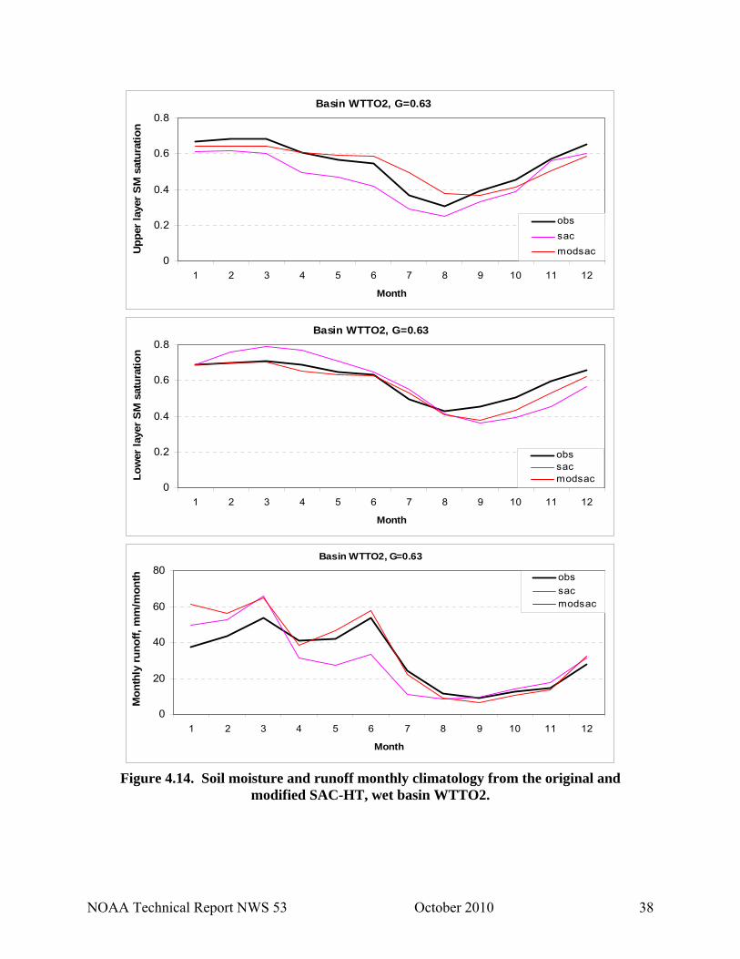
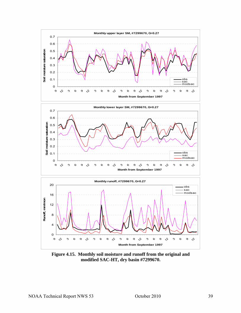
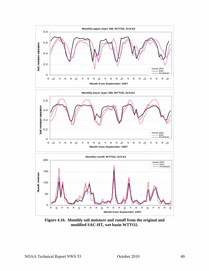
Overall, the modified version out-performs the original SAC-HT for dry basins with less benefit for wet basins, Table 4.7. As expected, soil moisture simulations at the lower layer are much better from the modified version; percent of the root mean square errors are better from the modified version for all 13 basins. Most statistics for soil moisture at the upper layer and runoff are better from the modified version; 9 of 13 basins perform consistently better. The seasonal variability of soil moisture and runoff compared to measurements can be seen in Figures 4.13 and 4.14 for dry and wet basins, respectively. Similar plots for monthly soil moisture and runoff are shown in Figures 4.15 and 4.16.
Table 4.7. Average statistics from the original and modified versions from 13 tested basins.
Highlighted values show better statistics
Version RMSE Bias AbsErr R NS %RMSE %Abs
Bias
Monthly runoff
Original 8.09 1.22 5.51 0.83 0.78 85.9 35.8
Modified 7.11 0.85 4.51 0.80 0.83 67.8 21.4
Daily upper layer (0-25 cm) soil saturation
Original 0.118 0.031 0.096 0.83 0.16 96.2 21.1
Modified 0.106 0.047 0.088 0.81 0.32 86.8 19.0
Daily lower layer (25-75 cm) soil saturation
Original 0.154 -0.020 0.132 0.75 -0.87 147.7 28.6
Modified 0.096 0.014 0.079 0.85 0.27 95.9 14.4
NOAA Technical Report NWS 53 October 2010 37
Basin 7299670, G=0.27
0
0.1
0.2
0.3
0.4
0.5
0.6
1 2 3 4 5 6 7 8 9 10 11 12
Month
Uppe
r lay
er S
M s
atur
atio
n
obssacmodsac
Basin 7299670, G=0.27
0
0.1
0.2
0.3
0.4
0.5
0.6
1 2 3 4 5 6 7 8 9 10 11 12
Month
Low
er la
yer S
M s
atur
atio
n
obssacmodsac
Basin 7299670, G=0.27
0
2
4
6
8
10
12
1 2 3 4 5 6 7 8 9 10 11 12
Month
Mon
thly
runo
ff, m
m/m
onth obs
sacmodsac
Figure 4.13. Soil moisture and runoff monthly climatology from the original and
modified SAC-HT, dry basin #7299670.
NOAA Technical Report NWS 53 October 2010 38
Basin WTTO2, G=0.63
0
0.2
0.4
0.6
0.8
1 2 3 4 5 6 7 8 9 10 11 12
Month
Uppe
r lay
er S
M s
atur
atio
n
obssacmodsac
Basin WTTO2, G=0.63
0
0.2
0.4
0.6
0.8
1 2 3 4 5 6 7 8 9 10 11 12
Month
Low
er la
yer S
M s
atur
atio
n
obssacmodsac
Basin WTTO2, G=0.63
0
20
40
60
80
1 2 3 4 5 6 7 8 9 10 11 12
Month
Mon
thly
runo
ff, m
m/m
onth obs
sacmodsac
Figure 4.14. Soil moisture and runoff monthly climatology from the original and
modified SAC-HT, wet basin WTTO2.
NOAA Technical Report NWS 53 October 2010 39
Monthly upper layer SM, #7299670, G=0.27
0
0.1
0.2
0.3
0.4
0.5
0.6
0.7
9 12 3 6 9 12 3 6 9 12 3 6 9 12 3 6 9 12 3 6 9 12
Month from September 1997
Soil
moi
stur
e sa
tura
tion
obssacmodsac
Monthly lower layer SM, #7299670, G=0.27
0
0.1
0.2
0.3
0.4
0.5
0.6
0.7
9 12 3 6 9 12 3 6 9 12 3 6 9 12 3 6 9 12 3 6 9 12
Month from September 1997
Soil
moi
stur
e sa
tura
tion
obssacmodsac
Monthly runoff, #7299670, G=0.27
0
4
8
12
16
20
9 12 3 6 9 12 3 6 9 12 3 6 9 12 3 6 9 12 3 6 9 12
Month from September 1997
Runo
ff, m
m/m
on
obssacmodsac
Figure 4.15. Monthly soil moisture and runoff from the original and
modified SAC-HT, dry basin #7299670.
NOAA Technical Report NWS 53 October 2010 40
Monthly upper layer SM, WTTO2, G=0.63
0
0.2
0.4
0.6
0.8
9 12 3 6 9 12 3 6 9 12 3 6 9 12 3 6 9 12 3 6 9 12
Month from September 1997
Soil
moi
stur
e sa
tura
tion
obssacmodsac
Monthly lower layer SM, WTTO2, G=0.63
0
0.2
0.4
0.6
0.8
9 12 3 6 9 12 3 6 9 12 3 6 9 12 3 6 9 12 3 6 9 12Month from September 1997
Soil
moi
stur
e sa
tura
tion
obssacmodsac
Monthly runoff, WTTO2, G=0.63
0
50
100
150
200
9 12 3 6 9 12 3 6 9 12 3 6 9 12 3 6 9 12 3 6 9 12
Month from September 1997
Runo
ff, m
m/m
on
obssacmodsac
Figure 4.16. Monthly soil moisture and runoff from the original and
modified SAC-HT, wet basin WTTO2.

NOAA Technical Report NWS 53 October 2010 41
Water subtraction from the original and modified SAC-HT. The modified SAC-HTCR water subtraction from the soil depends much on the canopy resistance factors listed in Section 3. Examples of the seasonal variability of all resistance factors and the plant coefficient that combines all these effects are shown in Figures 4.17 and 4.18 for dry and wet basins, respectively.
0
0.1
0.2
0.3
0.4
0.5
0.6
0 30 60 90 120 150 180 210 240 270 300 330 360
Time, days from January 1, 1996
Plan
t coe
ffici
ent,
pc
0
0.2
0.4
0.6
0.8
1
0 30 60 90 120 150 180 210 240 270 300 330 360
Time, days from January 1, 1996
Stom
atal
resi
stan
ce fa
ctor
s rsm
rsc
0
0.2
0.4
0.6
0.8
1
0 30 60 90 120 150 180 210 240 270 300 330 360
Time, days from January 1, 1996
Stom
atal
resi
stan
ce fa
ctor
s
rct
rcq
Figure 4.17. Seasonal variability of all resistance factors and estimated plant coefficient for
very dry basin #7300500, climate index=0.27. Resistance factors notation: rsm – soil moisture, rsc – solar radiation, rct – air temperature, rcq – humidity.
NOAA Technical Report NWS 53 October 2010 42
0
0.1
0.2
0.3
0.4
0.5
0.6
3 33 63 93 123 153 183 213 243 273 303 333 363
Time, days from January 1, 1996
Plan
t coe
ffici
ent,
pc
0
0.2
0.4
0.6
0.8
1
0 30 60 90 120 150 180 210 240 270 300 330 360
Time, days from January 1, 1996
Stom
atal
resi
stan
ce fa
ctor
s rsm
rsc
0
0.2
0.4
0.6
0.8
1
0 30 60 90 120 150 180 210 240 270 300 330 360
Time, days from January 1, 1996
Stom
atal
resi
stan
ce fa
ctor
s
rct
rcq
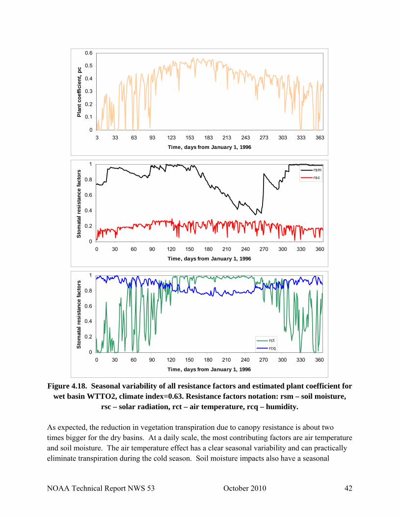
Figure 4.18. Seasonal variability of all resistance factors and estimated plant coefficient for
wet basin WTTO2, climate index=0.63. Resistance factors notation: rsm – soil moisture, rsc – solar radiation, rct – air temperature, rcq – humidity.
As expected, the reduction in vegetation transpiration due to canopy resistance is about two times bigger for the dry basins. At a daily scale, the most contributing factors are air temperature and soil moisture. The air temperature effect has a clear seasonal variability and can practically eliminate transpiration during the cold season. Soil moisture impacts also have a seasonal
NOAA Technical Report NWS 53 October 2010 43
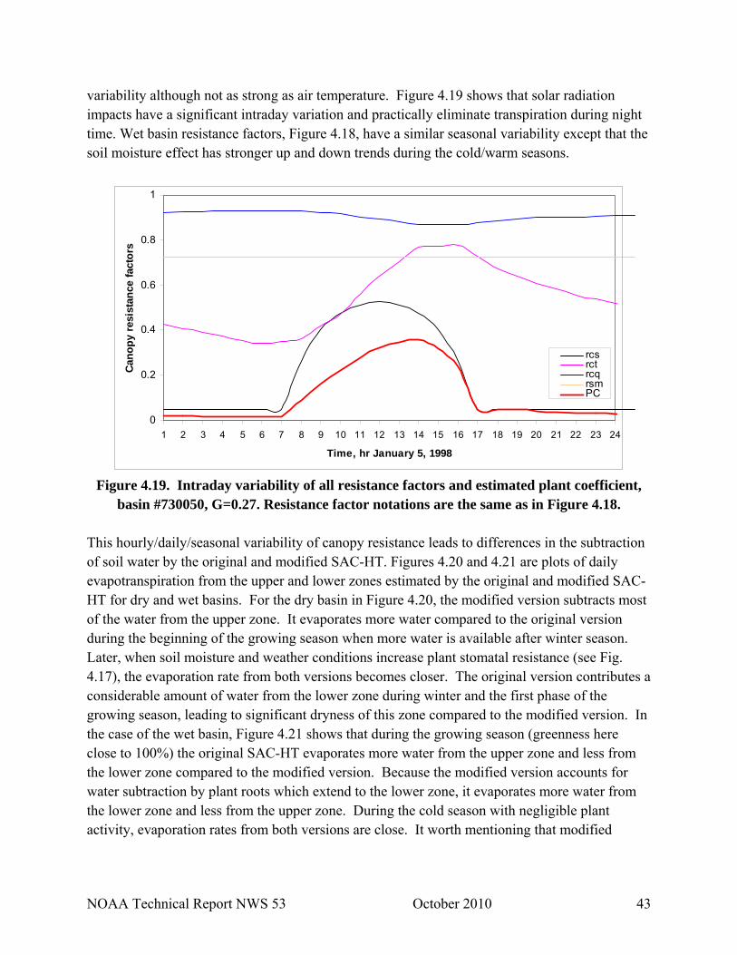
variability although not as strong as air temperature. Figure 4.19 shows that solar radiation impacts have a significant intraday variation and practically eliminate transpiration during night time. Wet basin resistance factors, Figure 4.18, have a similar seasonal variability except that the soil moisture effect has stronger up and down trends during the cold/warm seasons.
0
0.2
0.4
0.6
0.8
1
1 2 3 4 5 6 7 8 9 10 11 12 13 14 15 16 17 18 19 20 21 22 23 24
Time, hr January 5, 1998
Cano
py re
sist
ance
fact
ors
rcsrctrcqrsmPC
Figure 4.19. Intraday variability of all resistance factors and estimated plant coefficient,
basin #730050, G=0.27. Resistance factor notations are the same as in Figure 4.18. This hourly/daily/seasonal variability of canopy resistance leads to differences in the subtraction of soil water by the original and modified SAC-HT. Figures 4.20 and 4.21 are plots of daily evapotranspiration from the upper and lower zones estimated by the original and modified SAC-HT for dry and wet basins. For the dry basin in Figure 4.20, the modified version subtracts most of the water from the upper zone. It evaporates more water compared to the original version during the beginning of the growing season when more water is available after winter season. Later, when soil moisture and weather conditions increase plant stomatal resistance (see Fig. 4.17), the evaporation rate from both versions becomes closer. The original version contributes a considerable amount of water from the lower zone during winter and the first phase of the growing season, leading to significant dryness of this zone compared to the modified version. In the case of the wet basin, Figure 4.21 shows that during the growing season (greenness here close to 100%) the original SAC-HT evaporates more water from the upper zone and less from the lower zone compared to the modified version. Because the modified version accounts for water subtraction by plant roots which extend to the lower zone, it evaporates more water from the lower zone and less from the upper zone. During the cold season with negligible plant activity, evaporation rates from both versions are close. It worth mentioning that modified
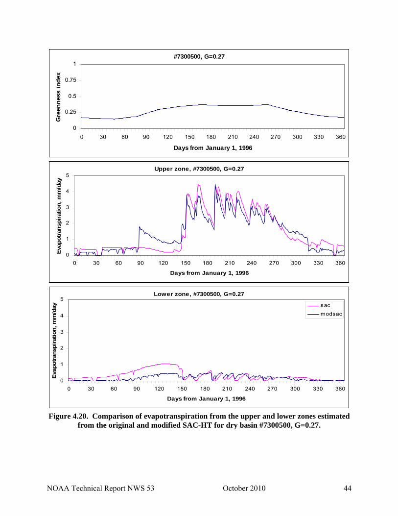
NOAA Technical Report NWS 53 October 2010 44
#7300500, G=0.27
0
0.25
0.5
0.75
1
0 30 60 90 120 150 180 210 240 270 300 330 360
Days from January 1, 1996
Gre
enne
ss in
dex
Upper zone, #7300500, G=0.27
0
1
2
3
4
5
0 30 60 90 120 150 180 210 240 270 300 330 360
Days from January 1, 1996
Evap
otra
nspi
ratio
n, m
m/d
ay
Lower zone, #7300500, G=0.27
0
1
2
3
4
5
0 30 60 90 120 150 180 210 240 270 300 330 360
Days from January 1, 1996
Evap
otra
nspi
ratio
n, m
m/d
ay sac
modsac
Figure 4.20. Comparison of evapotranspiration from the upper and lower zones estimated
from the original and modified SAC-HT for dry basin #7300500, G=0.27.

NOAA Technical Report NWS 53 October 2010 45
WTTO2, G=0.63
0
0.25
0.5
0.75
1
0 30 60 90 120 150 180 210 240 270 300 330 360
Days from January 1, 1996
Gre
enne
ss in
dex
Upper zone, WTTO2, G=0.63
0
1
2
3
4
5
0 30 60 90 120 150 180 210 240 270 300 330 360
Days from January 1, 1996
Evap
otra
nspi
ratio
n, m
m/d
ay
Lower zone, WTTO2, G=0.63
0
1
2
3
4
5
0 30 60 90 120 150 180 210 240 270 300 330 360
Days from January 1, 1996
Evap
otra
nspi
ratio
n, m
m/d
ay sac
modsac
Figure 4.21. Comparison of evapotranspiration from the upper and lower zones estimated
from the original and modified SAC-HT for wet basin WTTO2, G=0.63.
NOAA Technical Report NWS 53 October 2010 46
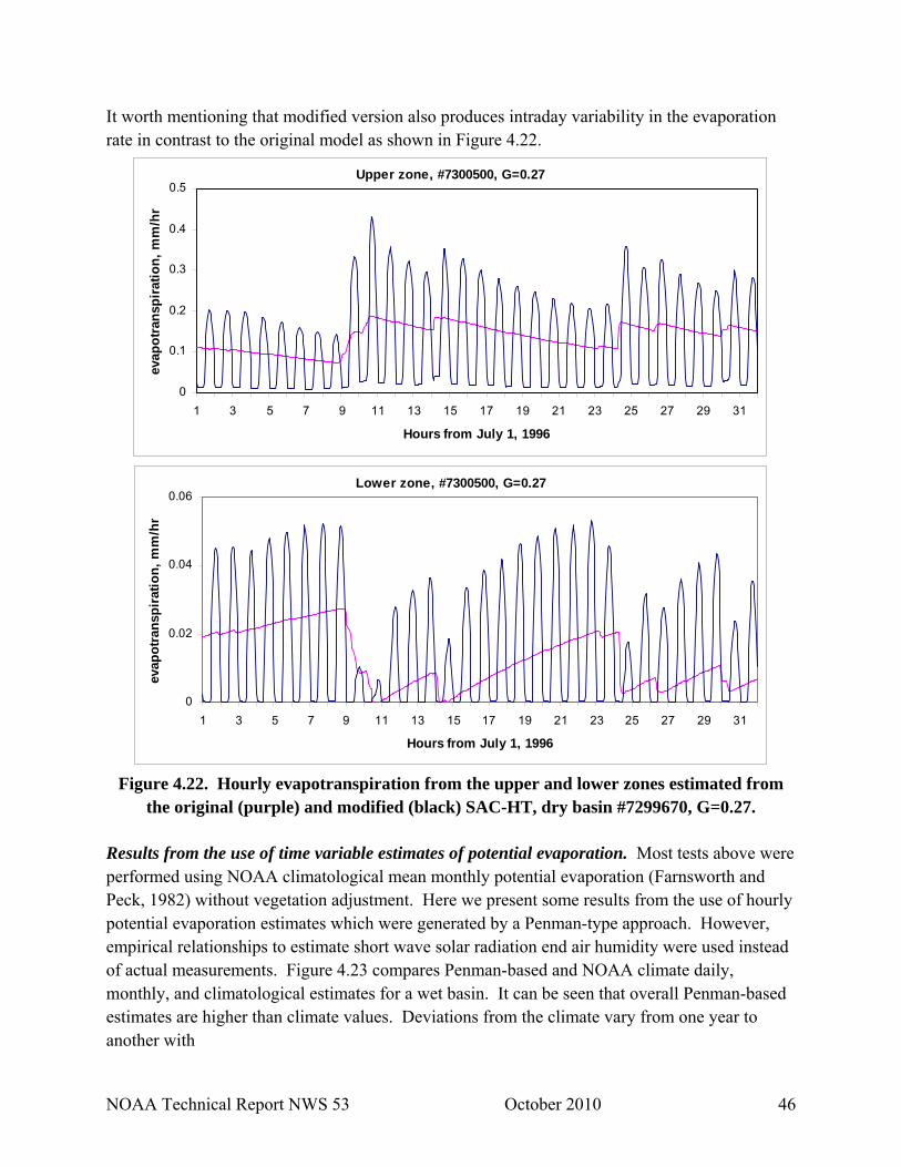
It worth mentioning that modified version also produces intraday variability in the evaporation rate in contrast to the original model as shown in Figure 4.22.
Upper zone, #7300500, G=0.27
0
0.1
0.2
0.3
0.4
0.5
1 3 5 7 9 11 13 15 17 19 21 23 25 27 29 31
Hours from July 1, 1996
evap
otra
nspi
ratio
n, m
m/h
r
Lower zone, #7300500, G=0.27
0
0.02
0.04
0.06
1 3 5 7 9 11 13 15 17 19 21 23 25 27 29 31
Hours from July 1, 1996
evap
otra
nspi
ratio
n, m
m/h
r
Figure 4.22. Hourly evapotranspiration from the upper and lower zones estimated from
the original (purple) and modified (black) SAC-HT, dry basin #7299670, G=0.27.
Results from the use of time variable estimates of potential evaporation. Most tests above were performed using NOAA climatological mean monthly potential evaporation (Farnsworth and Peck, 1982) without vegetation adjustment. Here we present some results from the use of hourly potential evaporation estimates which were generated by a Penman-type approach. However, empirical relationships to estimate short wave solar radiation end air humidity were used instead of actual measurements. Figure 4.23 compares Penman-based and NOAA climate daily, monthly, and climatological estimates for a wet basin. It can be seen that overall Penman-based estimates are higher than climate values. Deviations from the climate vary from one year to another with

NOAA Technical Report NWS 53 October 2010 47
0
2
4
6
8
10
12
1 4 7 9 12 3 6 9 12 3 6 9 12 3 6 9 12 3 6 9 12 3 6 9 12 3 6 9 12Month (Jan. 1996 - Dec. 2002)
PET,
mm
/day
OHD ClimatePenman
0
50
100
150
200
250
300
350
1 5 9 1 5 9 1 5 9 1 5 9 1 5 9 1 5 9 1 5 9Month (Jan. 1996 - Dec. 2002)
Mon
thly
PET
, mm
/mon
0
50
100
150
200
250
300
1 2 3 4 5 6 7 8 9 10 11 12
Month
Mon
thly
PET
OHDPenman
Figure 4.23. Daily, monthly and climatological potential evaporation estimated from OHD
monthly climate and from modified Penman approach for wet basin WTTO2.

NOAA Technical Report NWS 53 October 2010 48
the maximum change by about 40% of the NOAA climate amplitude. Simulation results from the modified SAC-HT after replacement of climate potential evaporation by hourly penman-based estimates are shown in Table 4.7.
Table 4.7. Ten basin- average statistics from simulations using NOAA climate and penman based potential evaporation estimates with and without adjustment
Variable NOAA Climate Penman Penman adjusted
%RMSE %Bias R %RMSE %Bias R %RMSE %Bias R
Upper SM
81.2 16.6 0.82 82.6 12.3 0.79 81.0 11.9 0.77
Lower SM
78.0 9.8 0.86 126.3 22.7 0.82 82.1 9.7 0.82
Runoff
72.9 24.6 0.79 91.2 62.1 0.74 75.0 29.3 0.77
Overall statistics are worse for the Penman-based simulations although the %Bias for the upper layer is even slightly better. Lower layer soil moisture and runoff errors from the Penman-based simulations are consistently worse for all basins except one. As can be expected, lower layer soil moisture and runoff is consistently underestimated, Figures 4.24 and 4.25, because the Penman-based evaporation is higher. Upper zone soil moisture errors are rather close except for the wettest basins where the Penman-based errors are much higher.

NOAA Technical Report NWS 53 October 2010 49
Upper layer (0-25cm) soil moisture ratio
0.0
50.0
100.0
150.0
0.26 0.27 0.27 0.3 0.33 0.340 0.45 0.51 0.59 0.63
Greennees Index
%R
MSE
Lower layer (25-75cm) soil moisture ratio
0.0
50.0
100.0
150.0
200.0
7300000 7300500 7299670 7316500 7148400 7325000 7177500 7334000 ELDO2 WTTO2
Basin ID
%R
MSE
Monthly runoff, mm/month
0.0
25.0
50.0
75.0
100.0
125.0
BSNID 7300000 7300500 7299670 7316500 7148400 7325000 7177500 7334000 ELDO2
Basin ID
%R
MSE
modsacpenpenadj
Figure 4.24. Comparison of %RMSE of soil moisture saturation and monthly runoff from the modified SAC-HTCR using different potential evaporation: OHD Climate
(modsac), Penman-based (pen), and adjusted Penman (penadj).

NOAA Technical Report NWS 53 October 2010 50
Upper layer (0-25cm) soil moisture ratio
-30.0
-20.0
-10.0
0.0
10.0
20.0
30.0
40.0
0.26 0.27 0.27 0.3 0.33 0.340 0.45 0.51 0.59 0.63
Greennees Index
%B
ias
Lower layer (25-75cm) soil moisture ratio
-40.0
-30.0
-20.0
-10.0
0.0
10.0
20.0
30.0
7300000 7300500 7299670 7316500 7148400 7325000 7177500 7334000 ELDO2 WTTO2
Basin ID
%B
ias
Monthly runoff, mm/month
-100.0
-80.0
-60.0
-40.0
-20.0
0.0
20.0
40.0
7300000 7300500 7299670 7316500 7148400 7325000 7177500 7334000 ELDO2 WTTO2
Basin ID
%Bi
as
modsacpenpenadj
Figure 4.25. Comparison of %Bias of soil moisture saturation and monthly runoff from the modified SAC-HTCR using different potential evaporation: OHD Climate
(modsac), Penman-based (pen), and adjusted Penman (penadj).

NOAA Technical Report NWS 53 October 2010 51
Comparison of Penman-based and NOAA climate annual potential evaporation (Figure 4.26) suggests a strong near linear correlation with R2 = 0.87 between their ratio, Kr, and annual average greenness index, G:
929.0477.0 +⋅−= GK r (4.1) where Kr is the ratio of NOAA climate- to Penman- based potential evaporation.
0.60
0.65
0.70
0.75
0.80
0.85
0.2 0.3 0.4 0.5 0.6 0.7
Greennees, G
r pt =
PT o
hd/P
Tpen
man
rpt = - 0.477*G+0.929R2 = 0.87
Figure 4.26. Dependency of NOAA and Penman annual PET ratio on
Greenness estimated from 10 Oklahoma basins.
The drier a basin is the closer Kr NOAA climate and Penman-based values are. Simulations with the use of adjusted Penman-based potential evaporation by a ratio from Eq. (4.1) were performed for the same test basins. Statistics are shown in Table 4.7 and Figures 4.24 and 4.25. Error and bias are close to those from NOAA climate-based simulation statistics for most basins although a few outliers are present. This adjustment can be used as an a priori estimate; however, minor adjustment may be needed for some basins.
NOAA Technical Report NWS 53 October 2010 52
5. Research findings The purpose of this project was to develop and evaluate an enhanced version of the SAC-HT model. In this enhancement, the canopy resistance parameterization from the Noah land surface model was incorporated into the SAC-HT evapotranspiration component for more physically-based estimation of water balance components, specifically evapotranspiration, runoff, and soil moisture. The main changes were to the upper and lower zone soil water subtraction and redistribution processes. The new version explicitly estimates transpiration from the rooting zone, direct evaporation and condensation from bare soil, and evaporation from the canopy surface. To be compatible with the SAC-HT structure and input data requirements at the RFCs, the canopy resistance formulation was reduced to require only precipitation and air temperature data. Available empirical temperature-based relationships for short wave solar radiation and air humidity were introduced to achieve this goal. Tests for a number of world-wide sites showed reasonable agreement between estimated and observed solar radiation even at an hourly time scale. Plant coefficients that control transpiration rate estimated using reduced formulation of the canopy resistance agreed well with plant coefficients estimated from the original Noah formulation. A mixed soil moisture redistribution mechanism was implemented that combines a SAC-HT percolation-based formulation for free water exchange and a Noah Richards-based formulation for tension water exchange. This approach allows tension water exchanges between upper and lower zones which were not possible in the original SAC-HT. To make the model flexible to run with different sources of the potential evaporation, e.g., monthly NOAA climate data which do not account for time variable wind, a wind speed adjustment factor was introduced to modify the potential evaporation. In this approach, wind speed time series are used to rescale monthly-type climate potential evaporation into variables at simulation time step values. We used a logistic dose-response curve that defines the cumulative amount of roots above a profile depth to define root distribution and rooting depth. It allows reducing complexity with implementation of Noah fixed formulation of rooting zone into spatially variable SAC-HTCR soil layer depths. Point/profile-type and lumped basin-type tests were performed in the Oklahoma Mesonet region. New version simulations were compared with the original model and measured data where available. A priori SAC-HT and introduced Noah-related parameters were used without
NOAA Technical Report NWS 53 October 2010 53
calibration. Only one parameter, the minimum stomatal resistance that controls transpiration rate, was manually adjusted to be consistent with NOAA potential evaporation climate data. Profile-type soil moisture simulations with the modified version show consistent improvement at all soil layers compared to the results from the original SAC-HT. Somewhat lower correlation at the upper soil layer is seen from the modified version. Lower variability at seasonal scale from the modified version may cause this behavior. This problem is addressed in basin-type tests. Thirteen basins were selected for lumped basin tests which covered as many as possible land cover classes and basin wetness values. No routing was used in these tests. Recent version of RDHM does not have definition of new Noah introduced parametric grids. Therefore, vegetation and soil texture related properties were estimated from basin average vegetation and soil classes. It leads to some inconsistency in average basin properties. A first set of simulations was generated using the Noah-recommended non-linear option of bare soil evaporation and vegetation dependent parameters including the minimum stomatal resistance parameter. NOAA monthly climate of potential evaporation was used as an input without vegetation adjustment. The modified version overall produced much more runoff and much wetter soil. Only lower layer soil moisture statistics were somewhat close to the original SAC-HT with an overestimation tendency compared to underestimation from the original version. Much better agreement was achieved for wetter basins where %Bias and %RMSE are better than from the original version for some basins. The most probable cause of overestimation was an overly high value of the Noah-prescribed minimum stomatal resistance, e.g. 400s/m for open shrubland. Use of climatological potential evaporation may have also contributed to this overestimation. However, simulations with the use of Penman-based potential evaporation showed some improvement but there was still significant overestimation of both runoff and soil moisture. Climatological plots for dry basins suggested that soil moisture dynamics, specifically at the upper soil layer, could not reproduce a seasonal pattern of soil moisture measurements. During the growing season, water subtraction for transpiration was too low leading to soil moisture saturation close to the cold season level. The next set of simulations was generated using manually adjusted minimum stomatal resistance parameter that removed significant biases in soil moisture and runoff. Adjusted values of this parameter were kept the same for all basins in the same vegetation class. The fitting process shows that minimum stomatal resistance parameter depends not only vegetation class but also on wetness. The parameter is much lower for wet basins with climate index above 0.5 for most classes (we do not have basins with forest classes) in the range of 40 – 5 s/m that agrees with reported values in publications. In addition, an option to switch from non-linear (lower rate evaporation) to linear (higher rate evaporation) bare soil evaporation is introduced that affects mostly dry basins. A threshold greenness fraction of 0.23 is selected as a switch mechanism.

NOAA Technical Report NWS 53 October 2010 54
6. Conclusions We identify the following conclusions: More physically consistent water subtraction for evapotranspiration from the upper and lower layers was achieved by implementing vegetation effects based on the canopy resistance parameterization. A number of changes to the Noah parameterization were needed to achieve acceptable results with the SAC-HTCR runoff generation mechanism. Overall, the modified version out-performed the original SAC-HT for dry basins with less benefit for wet basins. As expected, soil moisture simulations at the lower layer were much better from the modified version; all statistics were better from modified version for all 13 basins. Most statistics for soil moisture at the upper layer and runoff were better from the modified version; 9 of 13 basins perform consistently better. Also, the modified version produced better monthly climate patterns compared to the patterns from the original version. The rate of evapotranspiration proved to be very sensitive to the minimum stomatal resistance and water subtraction from bare soil. It may require some balance tuning for a specific basin. It also can simplify the use of potential evaporation sources other than the NOAA climatic monthly means. The modified SAC-HTCR version obviates the need to specify and calibrate the standard 12 monthly potential evaporation adjustment factors that account for vegetative activity. Some promising results were seen from the use of dynamical potential evaporation instead of the NOAA climatic monthly means. Penman-type estimates which were based only on the use of temperature data and scaled to NOAA climate values led to reasonable soil moisture and runoff results. The adjustment factors to the Penman estimates were calculated from previously derived relationships applied to all basins. 7. Recommendations Development of the modified version of SAC-HT highlighted several areas worthy of continued investigation. We identify items which relate to software integration and others related to the implementation of the new physics into the SAC-HTCR environment. Software integration:
NOAA Technical Report NWS 53 October 2010 55
The modified SAC-HTCR needs to be implemented into the CHPS version as a module for lumped and distributed modeling. Lumped and distributed applications of the modified SAC-HTCR will require the capability to ingest and process the gridded data sets discussed in Section 3.4. Because the HL-RDHM software that was used as the basic environment for implementing the Noah evapotranspiration component was in transition to the CHPS/FEWS system, the project requirement was not to introduce changes to the higher level HL-RDHM drivers. As a result, the capability of the modified HL-RDHM software package at this stage did not allow a simple streamline application, which limited its testing capability. Incorporate new Noah-based parameter sets into CHPS. Add ability to ingest observations of solar radiation and meteorological variables similar to the Noah model. Science items: The HL-RDHM software limitations led to some problems with the evaluation of the new version of the SAC-HTCR. First, all tests/evaluations were performed using point or lumped approaches. Second, the Noah parameterization introduces a number of new parametric grids which are not defined in the most recent HL-RDHM. Therefore, basin average classes were used instead of an average of the individual physical properties themselves. This application can lead to an inconsistency in soil-vegetation average classes because classes are not continuous monotonic properties. Because of lack of routing, time scale of basin tests of runoff were restricted to monthly averages, which are suitable for water balance analyses. Water redistribution in the modified version is now different from the original. During floods, the dynamics of the water balance components are changing at a rather high time scale resolution. To be sure that the new mechanism works properly at different scales, higher resolution tests need to be performed. Therefore, the CHPS/FEWS version of the HL-RDHM software needs to be modified to fully implement the modified SAC-HTCR. Further work is necessary to examine the Noah vegetation parameters, with special attention being paid to the minimum stomatal resistance Rs,min. Tests herein suggested that some Noah- defined parameters do not lead to reasonable results at different vegetation classes and basin wetnesses. Adjustment to the resistance parameter was made for a limited region with limited vegetation classes. Further testing is needed to be performed in regions with other types of vegetation such as forested areas. Tests should be performed to identify and evaluate sensitive parameters in these other regions. Recently, a number of new approaches in derivation of the potential evaporation have been under development. It would be advantageous to evaluate these approaches with the modified SAC-HTCR that is more capable to use different sources of this variable input.

NOAA Technical Report NWS 53 October 2010 56
8. References
Anderson, E. A., 1973. National Weather Service River Forecast System – Snow Accumulation and Ablation Model. NOAA Technical Memorandum NWS HYDRO-17, U.S. Department of Commerce, NOAA, NWS, Silver Spring, MD. Bristow, K. L., and Campbell, G. S., 1984. On the relationship between incoming solar radiation and daily maximum and minimum temperature. Agricultural and Forest Meteorology, 31, 159-166. Chen, F., K. Mitchell, J. Schaake, Y. Xue, H.-L. Pan, V. Koren, Q. Y. Duan, M. Ek, and A. Betts, 1996. Modeling of land-surface evaporation by four schemes and comparison with FIFE observations. JGR, Vol. 101, No. D3, 7251-7268. Chen, F., J. Dudhia, 2001: Coupling an advanced land surface hydrology model with the Penn State/NCAR MM5 modeling system. Part 1: Model description and implementation. Mon. Wea. Review 129, 569-586. Dickinson, R.E., 1984. Modeling evapotranspiration for three-dimensional global climate models. In Climate Processes and Climate Sensitivity, Geophysical Monograph Series, Vol. 29, AGU, Washington, D.C., 58-72. Dickinson, R. E., A. Henderson-Sellers, and P. J. Kennedy, 1993. Biosphere–Atmosphere Transfer Scheme (BATS) for the NCAR Community Climate Model. NCAR Tech. Note NCAR/TN-3871 STR, 78 pp Dingman, S. L., 2002. Physical Hydrology (second edition). Prentice Hall, Upper Saddle River, New Jersey 07458. Ek, M., and L. Mahrt, 1991. OSU 1-D PBL model user’s guide. Dept. of Atmos. Sci., Oregon State University, Corvallis. Ek, M.B., K.E. Mitchell, Y. Lin, E. Rogers, P. Grunmenn, V. Koren, G. Gayno, and J.D. Tarplay, 2003. Implementation of Noah land surface model advances in the National Centers for Environmental Prediction operational mesoscale Eta model. JGR, Vol. 108, D22, 12-1 – 12-11. Essery, R., Rutter, N., Pomeroy, J., Baxter, R., Stahli, M., Gustafsson, D., Barr, A., Bartlett, P., and Elder, K., 2009. SNOWMIP2: An evaluation of forest snow process simulations. BAMS, Vol. 90, No. 8, 1120-1135. Farnsworth, R.K., and Peck, E.L., 1982. Evaporation Atlas for the Contiguous 48 United States. NOAA Technical Report NWS 33, U.S. Department of Commerce. Gates, D. M., 1980. Biophysical Ecology. Springer-Verlag, New York. Hammon, R. W., 1963. Computation of direct runoff amounts from storm rainfall. Wellingford, Oxon, U.K., International Association of Scientific Hydrology, Publication 63. Hunt, L.A., L. Kuchar, C.J. Swanton, 1998. Estimation of solar radiation for use in crop modeling. Agricultural and Forest Meteorology, 91, 293-300. Jarvis, P.B., 1976. The interpretation of the variations in leaf water potential and stomatal conductance found in canopies in the field, Phil. Trans. Roy. Soc. Lond. B. 273, 593– 610. Jacquemin, B., and J. Noilhan 1990 Sensitivity study and validation of a land surface parametrization using the HAPEX-MOBILHY data set. Bound.-Lay. Meteor., 52, 93-134. Koren, V. I., 1991. Matematicheskie modeli v prognozach rechnogo stoka (Mathematical models in the river runoff forecasting). Gidrometeoizdat, Leningrad, 200pp.
NOAA Technical Report NWS 53 October 2010 57
Koren, V., J. Schaake, K. Mitchell, Q.-Y. Duan, F. Chen, J. M. Baker, 1999. A parameterization of snowpack and frozen ground intended for NCEP weather and climate models. JGR, Vol. 104, No. D16, 19,569-19,585. Koren, V., F. Moreda, S. Reed, M. Smith, 2006. Evaluation of a grid-based distributed hydrological model over a large area. IAHS Publ. 303, Predictions in Ungauged Basins: Promise and Progress (Proc. of symposium S7 held during the 7th IAHS Scientific Assembly at Foz do Iguacu, Brazil, April 2005), IAHS Publ. 303, pp. 47-56. Kuzmin, P. P., 1961. Process tayaniya sneznogo pokrova (Snowmelt processes). Gidrometeoizdat, Leningrad. Liu, D.L., B.J. Scott, 2001. Estimation of solar radiation in Australia from rainfall and
temperature observations. Agricultural and Forest Meteorology, 106, 41-59. Mesinger, F., DiMego, G., Kalnay, E., Mitchell, K., and co-authors, 2006. North American
Regional Reanalysis (NARR). Bulletin of the American Meteorological Society. Vol. 87, No. 3, 343-360.
Mizukami, N., 2010. Derivation of gridded seasonal snow melt factors over the United States for operational river forecasting, in preparation. Niyogi D., and Raman S., 1997. Comparison of four different stomatal resistance schemes using
FIFE data, Journal of Applied Meteorology, 36, 903 - 917. Noihlan, J., and S. Planton, 1989. A simple parameterization of land surface processes for meteorological models. Mon. Wea. Rev.,117, 536–549. Pan, H.-L., and L. Mahrt, 1987. Interaction between soil hydrology and boundary-layer development. Boundary Layer Meteorology, 38, 185-202. Penman, H.L., 1956. Evaporation: An introductory survey. Netherlands Journal of Agricultural Science 4, 7-29. Popov, E. G., 1948. Teplovoy balans i intensivnost snegotayaniya (Energy balance and snow melt rate). Trudy CIP, Vol. 9. Reed, S., Koren, V., Smith, M., Zhang, Z., Moreda, F., Seo, D.-J., and DMIP Participants, 2004. Overall distributed model intercomparison project results. Journal of Hydrology, Vol. 298, Nos. 1-4, 27-60 Schenk, H. J. and Jackson, R.B., 2002. Rooting depths, lateral root spreads, and belowground/aboveground allometries of plants in water limited ecosystems. Journal of Ecology, Vol. 90, 480-494. Sellars, P. J., Shuttleworth, W.J., Dorman, J.L., Dalcher, J. M., and Roberts, J.M., 1986. A simple biosphere model (SiB) for use within general circulation models. J. Atmos. Sci., 43, 505–531. Sellars, P., D. Randall, J. Collatz, J. Berry, C. Field, D. Dazlich, C. Zhang, G. Cellelo, and A. Bonuous, 1996. A revised land surface parameterization (SiB2) for atmospheric GCMs: Model formulation. J. of Climate, 9, 676-705. 1996 Smith, M., Koren, V., Zhang, Z., Zhang, Y., Reed, S., Cui, Z., Moreda, F., Anderson, E., Cosgrove, B., Mizukami, N., and DMIP 2 participants, 2010. Overall Results from the DMIP 2 Oklahoma Experiments, Journal of Hydrology, in preparation. Thompson, E.S., 1976. Computation of solar radiation from sky cover. Water Resources Research, vol. 12, No. 5, 859-865 Thornhwaite, C.W., 1948. An approach towards a rational classification of climate. Geographical Review 38: 55–94. doi:10.2307/210739

NOAA Technical Report NWS 53 October 2010 58
Thornton, P.E., S.W. Running, 1999. An improved algorithm for estimating incident daily solar radiation from measurements of temperature, humidity, and precipitation. Agricultural and Forest Meteorology, 93, 211-228. Xue, Y., P.J. Selers, J.L. Kinter III, J. Shukla, 1991. A simplified biosphere model for global climate studies. Journal of Climate, Vol. 4, 345-364. Zamora, R.J., F.M. Ralph, E. Clark, and Schneider, T., 2009. The NOAA Hydrometeorology Testbed Soil Moisture Observing Networks: Design, Instrumentation, and Preliminary Results. Submitted to Journal of Hydrometeorology.
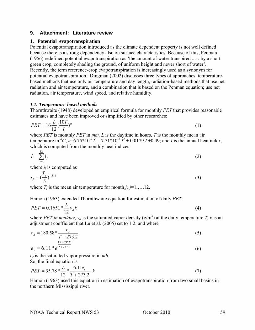
NOAA Technical Report NWS 53 October 2010 59
9. Attachment: Literature review 1. Potential evapotranspiration Potential evapotranspiration introduced as the climate dependent property is not well defined because there is a strong dependency also on surface characteristics. Because of this, Penman (1956) redefined potential evapotranspiration as ‘the amount of water transpired ..… by a short green crop, completely shading the ground, of uniform height and never short of water’. Recently, the term reference-crop evapotranspiration is increasingly used as a synonym for potential evapotranspiration. Dingman (2002) discusses three types of approaches: temperature-based methods that use only air temperature and day length, radiation-based methods that use net radiation and air temperature, and a combination that is based on the Penman equation; use net radiation, air temperature, wind speed, and relative humidity. 1.1. Temperature-based methods Thornthwaite (1948) developed an empirical formula for monthly PET that provides reasonable estimates and have been improved or simplified by other researches:
α)10(12
16ITLPET = (1)
where PET is monthly PET in mm, L is the daytime in hours, T is the monthly mean air temperature in oC; a=6.75*10-7 I3 – 7.71*10-5 I2 + 0.0179 I +0.49; and I is the annual heat index, which is computed from the monthly heat indices
∑=
=12
1jjiI (2)
where ij is computed as 514.1)
5( j
j
Ti = (3)
where Tj is the mean air temperature for month j: j=1,…,12. Hamon (1963) extended Thornthwaite equation for estimation of daily PET:
kvLPET d12*1651.0= (4)
where PET in mm/day, νd is the saturated vapor density (g/m3) at the daily temperature T, k is an adjustment coefficient that Lu et al. (2005) set to 1.2; and where
2.273*58.180
+=
Tes
dν (5)
3.237*269.17
*11.6 += TT
s ee (6) es is the saturated vapor pressure in mb. So, the final equation is
kT
eLPET s ⋅+
=2.273
11.6*
12*78.35 (7)
Hamon (1963) used this equation in estimation of evapotranspiration from two small basins in the northern Mississippi river.

NOAA Technical Report NWS 53 October 2010 60
1.2. Radiation-based methods Air moving over a homogeneous well-watered surface would become saturated, so the mass-transfer term in the Penman equation would disappear (Dingman, 2002). Evapotranspiration under these conditions is the equilibrium potential evapotranspiration (PETeq). Priestley and Taylor (1972) compared this evapotranspiration with values determined by energy-balance methods over well-watered surfaces and found a close fit if PETeq was multiplied by a factor β to give
)( γλρβ
+Δ⋅⋅⋅Δ⋅
=vw
RPET (8)
where Δ is the slope of saturation-vapor vs. temperature at the air temperature, Δ=(esat,s-esat,a)/(Ts-Ta), R is the net radiation, ρw is the water density, λv is the latent heat of vaporization, and γ is the psychometric constant. A number of field studies of evapotranspiration in humid regions have found β = 1.26, and theoretical examination has shown that that value in fact represents equilibrium evapotranspiration over well-watered surfaces under a wide range of conditions. Equation (8) uses only radiation and air temperature data. 1.3. Combination methods If the required data are available, the Penman equation can be used as a basic model:
)()1(
γλρρ
+Δ⋅⋅−⋅⋅⋅⋅+⋅Δ
=vw
asataa WeCcRPET (9)
where ca is the heat capacity of air [ca=10-3MJ/(kg* K)], ρa is the density of air, es is the saturation vapor pressure at the air temperature, Wa is the relative humidity of air as a ratio of its actual vapor pressure to its saturation vapor pressure, and Cat is the atmospheric conductance:
2
0
)][ln(25.6z
zzu
Cdm
aat −
⋅= (10)
where ua is wind speed, zm is the measurement height assumed here 2m, zd is the zero-plane displacement, and z0 is the roughness height. They can be approximately related to the height of vegetation, zveg, as
vegd zz ⋅= 7.0 (11)
vegzz ⋅= 1.00 (12) Equations (11), (12) can be used to generate a relation between atmospheric conductance and wind speed for various values of zveg.
Monteith (1956) extended the Penman equation to represent the evapotranspiration rate from a vegetated surface by incorporating canopy conductance, Ccan:
)]/1([)1(
canatvw
asataa
CCWeCcR
PET+⋅+Δ⋅⋅
−⋅⋅⋅⋅+⋅Δ=
γλρρ
(13)
A big problem is the estimation of canopy conductance. Transpiration is a two-step process in which water molecules pass (1) from the stomata cavity to the leaf surface and (2) from the leaf surface into the atmosphere. Leaf conductance is determined by the number of stomata per unit area and size of the stomatal openings. Stomatal densities range from 10,000 to 100,000 stomata

NOAA Technical Report NWS 53 October 2010 61
per square centimeter of leaf surface, depending on species. Plants control the size of the stomatal openings, and hence leaf conductance, by the response of the guard cells. These cells have been found to respond to: light intensity, CO2 concentration, leaf-area vapor pressure difference, leaf temperature, and leaf water content. There are two basic approaches of estimation of leaf conductance, Cleaf, or canopy resistance, Rleaf, physiological and meteorological. Though physiological methods tend to mimic the physiological response to CO2 concentration, they are still empirical in nature and need not represent a casual relation. Niyogi and Raman (1997) tested few such schemes using FIFE observations. They observed much similarity in the model performances including simple and flexible scheme that uses the vapor pressure deficit approach :
ls
nasleaf COCO
Ad
eeCC
,2,2maxmin
6.11
−⋅
⋅⎟⎟⎠
⎞⎜⎜⎝
⎛ −−+= (14)
where Cmin is the minimal leaf conductivity assumed to be 0.01 mol/(m2s), CO2,s, and CO2,l are CO2 concentrations at the leaf surface and within the leaf respectively, es and ea are the saturated vapor pressure at the surface temperature and air temperature respectively, An is the photosynthesis rate, and dmax empirical parameter taken as 45 g/kg. Land surface models use mostly meteorological methods. These methods try to mimic stomatal opening responds to light intensity, CO2 concentration, leaf-area vapor pressure difference, leaf temperature, and leaf water content. Stewart (1988) developed a model for estimating hourly evapotranspiration that incorporates light intensity, leaf-area vapor pressure difference, leaf temperature, and leaf water content factors that determine leaf conductance (CO2 concentration effect was not included because it usually varies little with time):
)()()()(max θρ θ Δ⋅⋅Δ⋅⋅= fTffRfCC aTvpRleaf (15) where Cmax is the maximum value of leaf conductance [Dingman (2002) provides its values for principal land-cover types], R is incident short-wave radiation flux, Δρv is the humidity deficit (the difference between the saturated and actual absolute humidity of the air, calculated from vapor pressure and temperature), Ta is air temperature, and Δθ is the soil moisture deficit (the difference between the field capacity and the actual water content of the root zone). The fi in the equation are non-linear functions with values between 0 and 1:
)/(5.860_,........4.10457.11
78.12 2daymMJRifR
Rf R ≤≤+⋅⋅
= (16)
⎩⎨⎧
Δ≤Δ≤Δ⋅−
= 3
3
/01152.0_.....................,.........233.0/01152.00_...,.........6.661mkgifmkgif
fv
vv
fρρρ
ρ (17)
CTifTT
f aaa
T0
18.1
400_,.........691
)40(≤≤
−⋅= (18)
cmifef 4.80_,.....00119.01 81.0 ≤Δ≤⋅−= Δ⋅ θθθ (19)
While Stewart (1988) derived these functions only from one site data (a pine forest in southeast England), controlled studies indicate that their form is quite general (Jarvis, 1976). A vegetated surface like a grass, crop, or forest canopy can be thought as a large number of leaf conductances in parallel (Dingman, 2002). Thus, a reasonably uniform vegetated surface can be considered as a single ‘big leaf’ whose total conductance is proportional to the sum of the
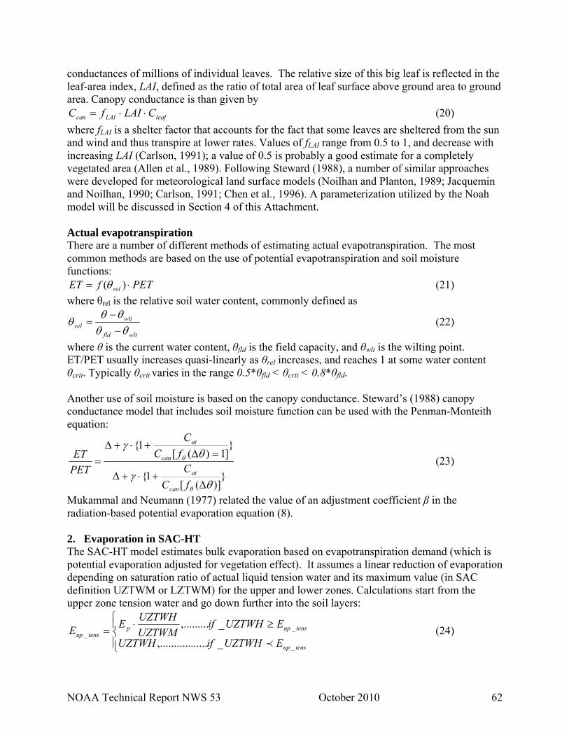
NOAA Technical Report NWS 53 October 2010 62
conductances of millions of individual leaves. The relative size of this big leaf is reflected in the leaf-area index, LAI, defined as the ratio of total area of leaf surface above ground area to ground area. Canopy conductance is than given by
leafLAIcan CLAIfC ⋅⋅= (20) where fLAI is a shelter factor that accounts for the fact that some leaves are sheltered from the sun and wind and thus transpire at lower rates. Values of fLAI range from 0.5 to 1, and decrease with increasing LAI (Carlson, 1991); a value of 0.5 is probably a good estimate for a completely vegetated area (Allen et al., 1989). Following Steward (1988), a number of similar approaches were developed for meteorological land surface models (Noilhan and Planton, 1989; Jacquemin and Noilhan, 1990; Carlson, 1991; Chen et al., 1996). A parameterization utilized by the Noah model will be discussed in Section 4 of this Attachment. Actual evapotranspiration There are a number of different methods of estimating actual evapotranspiration. The most common methods are based on the use of potential evapotranspiration and soil moisture functions:
PETfET rel ⋅= )(θ (21) where θrel is the relative soil water content, commonly defined as
wltfld
wltrel θθ
θθθ
−−
= (22)
where θ is the current water content, θfld is the field capacity, and θwlt is the wilting point. ET/PET usually increases quasi-linearly as θrel increases, and reaches 1 at some water content θcrit. Typically θcrit varies in the range 0.5*θfld < θcrit < 0.8*θfld. Another use of soil moisture is based on the canopy conductance. Steward’s (1988) canopy conductance model that includes soil moisture function can be used with the Penman-Monteith equation:
})]([
1{
}]1)([
1{
θγ
θγ
θ
θ
Δ+⋅+Δ
=Δ+⋅+Δ
=
fCC
fCC
PETET
can
at
can
at
(23)
Mukammal and Neumann (1977) related the value of an adjustment coefficient β in the radiation-based potential evaporation equation (8). 2. Evaporation in SAC-HT The SAC-HT model estimates bulk evaporation based on evapotranspiration demand (which is potential evaporation adjusted for vegetation effect). It assumes a linear reduction of evaporation depending on saturation ratio of actual liquid tension water and its maximum value (in SAC definition UZTWM or LZTWM) for the upper and lower zones. Calculations start from the upper zone tension water and go down further into the soil layers:
⎪⎩
⎪⎨⎧ ≥⋅=
tensup
tensupptensup
EUZTWHifUZTWH
EUZTWHifUZTWMUZTWHEE
_
__
_........,.........
_,.........
p (24)
NOAA Technical Report NWS 53 October 2010 63
Evaporation from the upper zone free water storage at potential demand rate reduced by tension water evaporation:
⎩⎨⎧ ≥−
=freeup
freeuptensuppfreeup EUZFWHifUZFWH
EUZFWHifEEE
_
___ _....,.........
_,.......p
(25)
Evaporation demand from the lower zone tension water reduced by upper zone evaporations: freeuptensupplop EEEE __, −−= (26)
and actual evaporation from the upper zone tension water:
⎪⎩
⎪⎨⎧ ≥
+⋅=
tenslo
tensloloptenslo
ELZTWHifLZTWH
ELZTWHifLZTWMUZTWM
LZTWHEE_
_,_
_..........................,.........
_,......
p (27)
The total evaporation from SAC-HT upper and lower zones not adjusted for impermeable area (evaporation from this area will be estimated separately) is the sum of the above components:
tenslofreeuptensupzone EEEE ___ ++= (28) There are two more components: riparian and evaporation from the variably impermeable area. Riparian evaporation directly from the river channel is
riverzoneprep FEEE ⋅−= )( (29) where Friver is a fraction of riparian area (model parameter). Variable impermeable area evaporation occurs from impermeable area storage at rate:
LZTWMUZTWMUZTWCEADIMC
EEEE tensupfreeuploptensupimp +
−−++= _
_,_ )( (30)
where ADIMC is additional impermeable area water content. The grand total evapotranspiration equals:
imprepzone EEPCTIMADIMPEE ++−−⋅= )1( (31) ADIMP and PCTIM are model parameters, additional and permanent impermeable area fractions respectively. 3. Parameterization of evaporation in the Noah land surface scheme
Actual evaporation estimation is based on the Penman equation adjusted by soil moisture and canopy resistance effects. It consists of three components: direct evaporation from the top soil layer, evaporation of precipitation intercepted by the canopy, and transpiration via canopy and roots. The Noah direct evaporation from the top soil layer (Ek et al. 2003), Edir, is estimated as a ratio of the potential evaporation similar to SAC-HT:
fx
spdir EE )()1(
min
min1
θθθθ
σ−−
⋅⋅−= (32)
where σ is the green vegetation fraction, Ep is the potential evaporation, θ1 is the soil moisture in the upper soil layer, θs and θmin are air dry (minimum) and saturation (porosity) soil moisture respectively, fx is an empirical coefficient; Ek et al. (2003) recommended value 2.
The wet canopy evaporation, Ec, is determined by

NOAA Technical Report NWS 53 October 2010 64
ncpc W
WEE )(
max
⋅⋅= σ (33)
where Wc is the intercepted canopy water content, Wmax is the maximum allowed canopy interception; Chen et al. (1996) recommended values Wmax= 0.5 mm and parameter n = 0.5. The intercepted canopy water budget is govern by
EPPt
Wd
c −−⋅=∂∂
σ (34)
If Wc exceeds Wmax, the excess precipitation, Pd, reaches the ground. Therefore actual surface precipitation equals Ps = (1-σ)P + Pd where P is measured precipitation.
The canopy evapotranspiration is determined by (Chen et al. 1996)
⎥⎥⎦
⎤
⎢⎢⎣
⎡⎟⎟⎠
⎞⎜⎜⎝
⎛−⋅⋅=
n
ccpt W
WBEE
max
1σ (35)
where Bc embodies canopy resistance. The factor (Wc/Wmax)n serves a weighting factor to suppress Et in favor of Ec as the canopy surface becomes increasingly wet. Noah model has two approaches for calculating the resistance term Bc.
The earlier Pan and Mahrt (1987) approach that explicitly accounts only for soil moisture stress: 4FPB cc = (36)
where Pc is a constant ‘plant coefficient’ between 0 and 1 depending on the vegetation species (typically around 0.8 and meant to crudely capture a minimal stomatal resistance effect). F4 is a soil moisture stress function also between 0 and 1:
∑= +−
⋅−=
2
1 214 ))((
)(i zzwltfld
ziwlt
ddd
Fθθθθ
(37)
where θ, θfld, θwlt are actual soil moisture, field capacity, and wilting point respectively, dz1 and dz2 are thickness of the upper and lower layers in m. Note to consider during implementation: the recent version has more than 2 layers; so, possibility to use more than 2 layers depending on the root zone depth should be investigated. Also, Chen and Dudhia (2001) used some kind of non-linear function not defined in the earlier paper (Chen et al., 1996). They used simple approach to extent evaporation beyond θfld ( θwlt) by simply decreasing (increasing) these threshold values: θfld=1/3*θs+2/3*θfld,est and θwlt=0.5*θwlt,est, where θfld,est and θwlt,est are values of field capacity and wilting point estimated from soil texture. The later extended version accounts for the most components of canopy resistance effects similar to Stewart (1989). The parameterization actually uses the electric-circuit analogy to combine canopy and atmospheric resistances linked in series:
rch
rc RRC
RB
/1/1Δ++
Δ+= (38)
NOAA Technical Report NWS 53 October 2010 65
where Δ depends on the slope of the saturation specific humidity curve, Ch is the surface exchange coefficient for heat and moisture, Rr is a function of surface air temperature, pressure, and Ch, and Rc is the total canopy resistance [including F4 defined in Eq. (37)]:
LAIFFFFR
R cc ⋅⋅⋅⋅=
4321
min, (39)
LAIRR
fwheref
fRRF
gl
gcc 255.0_.......,1/ max,min,
1 ⋅=+
+= (40)
])([11
2aas qTq
F−⋅+
=β
(41)
)(1 13 aref TTBF −−= (42)
where Rc,min and Rc,max are minimum and maximum [the cuticular resistance of the leaves from Dickinson et al. (1993)] stomatal resistance respectively [Chen et al., (1996) used 40 and 5000 s/m for its minimum and maximum values respectively], LAI is the leaf area index, Rgl is a limit value of 30 W m2 for a forest and of 100 W m2 for a crop, Rg is the solar radiation (the factor F1 represents the influence of the photosynthetically active radiation, assumed to be 0.55 of the solar radiation), β, B1, Tref are empirical parameters. Chen et al. (1996) used β=36.4, however, in other paper Chen and Dudhia (2001) provide a table of variable β (page 576) depending on 16 vegetation classes. Two other parameters are the same in both above papers: B1=0.0016, Tref=292 0K. Eq. (38), which accounts for the canopy effects on evapotranspiration includes the slope of the saturation specific humidity curve Δ that depends on air temperature and vapor pressure gradients. No vapor pressure data are used in SAC-HT. So, it is possible to simplify (38) by using Noilhan and Planton (1989) resistance approach:
ch
h
cac RC
CRR
B+
=+
=1
1 (43)
where Ra is the atmospheric resistance. This approach eliminates the use of the slope of the saturation specific humidity curve that requires additional input data. References Allen, R.G., M.E. Jensen, J.L. Wright, and R.D. Burman, 1989. Operational estimates of reference evapotranspiration. Agronomy Journal, 81, 650-662.
Carlson, T., 1991. Modeling stomatal resistance: an overview of the 1989 workshop at the Pensilvania State University. Agricultural and Forest Meteorology, 54, 103-106.
Chen, F., K. Mitchell, J. Schaake, Y. Xue, H.-L. Pan, V. Koren, Q. Y. Duan, M. Ek, and A. Betts, 1996. Modeling of land surface evaporation by four schemes and comparison with FIFE observations. JGR, vol. 101, D3, 7251-7268.
Chen, F., and J. Dudhia, 2001. Coupling an advance land surface-hydrology model with the Penn state-NCAR MM5 modeling system. Part I: Model implementation and sensitivity. Monthly Weather Review, vol. 129, 569-585.

NOAA Technical Report NWS 53 October 2010 66
Dingman, S. L., 2002. Physical Hydrology: Second edition. Prentice Hall, Upper Saddle River, New Jersey 07458, 646pp.
Ek, M.B., K.E. Mitchell, Y. Lin, E. Rogers, P. Grunmann, V. Koren, G. Gayno, 2003. Implementation of Noah land surface model advances in the National Centers for Environmental Prediction operational mesoscale Eta model. JGR, vol. 108, D22.
Hamon, R. W., 1963. Computation of direct runoff amounts from storm rainfall. Wellingford, Oxon, U.K., International Association of Scientific Hydrology, Publication 63.
Niyogi, D.S., S. Raman, 1997. Comparison of four different stomatal resistance schemes using FIFE observations. Journal of Applied Meteorology, vol. 36, issue 7, 1-13.
Jacquemin, B., and J. Noilhan, 1990. Sensitivity study and validation of a land surface parameterization using the HAPEX-MOBILHY data set. Boundary Layer Meteorology, 52, 93-134. Jarvis, P.G., 1976. The interpretations of the variations in leaf water potential and stomatal conductance found in canopies in the field. Royal Society of London Philosophical Transactions Series B 273, 593-610.
Monteith, J.L., 1965. Evaporation and environment. In New York, NY: Cambridge University Press, Proceedings of the 19th Symposium of the Society for Experimental Biology, 205-233.
Noilhan, J., S. Planton, 1989. A simple parameterization of land surface processes for meteorological models. Monthly Weather Review, 117, 536-549.
Lu, J., G. Sun, S.G. McNulty, and D.M. Amatya, 2005. A Comparison of six Potential Methods for Regional Use in the Southern United States. Journal of the American Water Resources Association, June, 2005, 621-633.
Priestley, C.H.B., and R.J. Taylor, 1972. On the assessment of surface heat flux and evaporation using large-scale parameters.Monthly Weather Review 100, 81-92.
Thornhwaite, C.W. (1948). "An approach towards a rational classification of climate". Geographical Review 38: 55–94. doi:10.2307/210739
Stewart, J.B., 1988. Modeling surface conductance of pine forest. Agricultural and Forest Meteorology, 43, 17-35.
Mukammal, E.I., H.H. Newmann, 1977. Application of the Priestley-Taylor evaporation model to asses the influence of soil moisture on the evaporation from a large weighing lysimeter and class A pen. Boundary-Layer Meteorology, 12, 243-256.