ModellingModelling SubsurfaceSubsurface FlowFlow −−not not whatwhat youyou seesee, , butbut whatwhat youyou imagineimagine

NilsNils--Otto KitterødOtto Kitterød

FEMLAB conference, Oslo October 13. 2005

Outline:

• teaching

• how to make COMSOL MULTIPHYSICS behave according to my concepts

• examples

Why focus on groundwater?

Important for societyGroundwater resources of the world

Major part of the world population are depending on groundwater

resources

The global water balance

~ 30 times more groundwater than water in the lakes

Groundwater flow is a boundary

value problem => measurements

unsaturated zone

saturated zone

Important for nature

Why focus on groundwater?

Groundwater: the liquid of life!interface to human society and science

groundwater flow contaminant transport

numerical simulation

concept ofgeology

Concept of flow:

Henri-Philibert-Gaspard Darcy

Darcy's experiments (1856):

∆h

∆x

A

Q ∝ A ∆h∆x

Darcy’s law:governs the laminar (nonturbulent) flow of fluids in homogeneous, porous media

→ Conservation of momentum

1. Conservation of momentum:

q = − K ∇h, where h = p/(ρg) + z

2. Conservation of mass:

+ N,∂ ( S0 h )

∂t− ∇⋅q= where S0 is specific storage [1/L],

and N is a sink/source term3. Constitutive relations:

e.g. if S0 is a function of h → Richards’ equation (not today!)or if ρ is a function of concentration of solute (later)

Here: Dupuit-Forchheimer assumption:∂ h∂z

= 0, which means 3D → 2Dbut qz ≠ 0

4. Boundary conditions and (if transient) initial conditions

Cross Section of the Gardermoen Delta

After K. Tuttle (1997)

100020003000

200

100

m a.s.l.

West meters East

05001:1

0100020003000

200

180

160

140

120

m a.s.l.

Bedrock

Delta Bottomsets

Delta Foresets

Delta Topsets

??

?

Kettle-hole

Ice-contactslope

1:~15

West meters East

From 1,2 we have: + N.∂ ( S0 h )

∂t∇⋅= K ∇h

where m is thickness of water saturated zonemS0 = S [-] is called storage coefficientmK = T [L2/T] is called transmissivity

For a confined aquifer:

m = top – bottom of aquifer

For an unconfined aquifer:

m = h – bottom of aquifer

H1H2

length of aquiferx

top

bottom m = const.

H1H2

length of aquiferx

bottomm = h(x,t)

From 3, life gets easier: + N,∂ ( mS0 h )

∂t∇⋅= mK ∇h

Remember (2): Q = Aq (L3/T)By using boundary integration in postprocessing, you get the water flow directly!

Transmissivity

Implement the Dupuit-Forchheimer assumption:

Remember (1): h(t0) ≠ 0if bottom = 0

Challenge: estimate Challenge: estimate effectiveeffective parametersparameters

The Boussinesq equation( )hT= ∇ −⋅∇∂∂

t( S h ) N(t)

in a way that the response h is reproduced according to the observations

where: T effective transmissivity (L2/T) S storage coefficient(-) h hydraulic head (L)t time (T)N(t) source/sink (L/T), infiltration or pumping

T = ∫ T(z) dz0

m

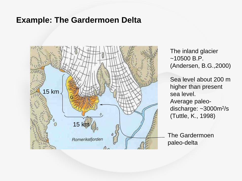
The inland glacier ~10500 B.P. (Andersen, B.G.,2000)

Sea level about 200 m higher than present sea level.Average paleo-discharge: ~3000m2/s (Tuttle, K., 1998)

Example: The Gardermoen Delta

The Gardermoenpaleo-delta

15 km

15 km

Trandum Delta Paleo-portal

Helgebostad Delta Paleo-portal

The Gardermoen Delta Today:

Gardermoen, grw. obs, eu89

1000

2000

3000

4000

5000

6000

7000

8000

9000

10000

11000

4000 5000 6000 7000 8000 9000 10000 11000 12000

UTM-East

UTM

-Nor

th

Paleo-distribution Channels Show Radial Flow:

Trandum Delta Paleo-portal

Helgebostad Delta Paleo-portal

x-profile

””The The GardermoenGardermoen Doughnut”Doughnut”

ii) Balance of mass:

c) QΑ = Nπl2 – Nπr2

d) Qr = – QΑ

2πr

i and ii): d(1/2 kh2) = N2

l2

rdr – r dr

i) Darcy’s law:

= q = – k dhdr

Qr

ma)

Qr = – d(1/2 kh2)dr

b) if m=h, then unconfined aquifer

R2 h2 R1

h1lSteady state modelfor R1 ≤ r ≤ l :

Repeat for l ≤ r ≤ R2

and eliminate l to get oneclosed form expression for h(r)

Plot observations of groundwater head as a function of radial distance from center:

let k = k(r)or H = H(r)

rR2 R1l

h2

h1

N

l

→

WRR(40) 2004http://folk.uio.no/nilsotto/PUBL/analytical_gilbert.pdf

where k = k1 – a(r-R1)

∫ 1r(k0-ar) dr

∫ r(k0-ar) dr

Two (simple) integrals:

(1)

(2)

rR2 R1 l

h2

h1

N

l

→

k1 k2

dh2 N l2

rk dr dr– rk=

Implement the solution as a function in MATLAB:

function[h] = funk_h_lin(radius, R1, R2, h1, h2, N, k_1, k_2)

minimum(hobs – hcalc) gives k1 at R1 and k2 at R2

function[h] = funk_h_lin(radius, R1, R2, h1, h2, N, k_1, k_2)

R2 h2

R1h1

l

Radial Duit-Forchheimer Solution where k=k(r)

Interpolation Functions:

R1R2

k1k2

Steady State Numerical SolutionandAnalytical Solution:

S=0.01

Precipitation event

1 3 5 7 9 11 13 15 17 19 21 23 25 27 29 31days from 27.09.2000

0.00

2.00

4.00

6.00

8.00

10.00

12.00

14.00

16.00

18.00

mm

/d

Transient Simulation

OK !But, what about the real aquifer?

Precipitation event

1 3 5 7 9 11 13 15 17 19 21 23 25 27 29 31days from 27.09.2000

0.00

2.00

4.00

6.00

8.00

10.00

12.00

14.00

16.00

18.00m

m/d

Transient boundary condition:

H1(t) = H1sin(t/day)

Conclusion:1) minor changes in h with N(t)2) not very sensitive to H1

Trandum Delta Paleo-portal

Helgebostad Delta Paleo-portal

188

180

190

190

188

188

Digitize boundary by using: GINPUT Graphical input from mouse.[X,Y] = GINPUT(N) gets N points from the current axes and returns the X- and Y-coordinates in length N vectors X and Y.

Spline interpolation

Make solid object by: s1 = geomcoerce('solid',{c});geomplot(s1);and import geometry in Comsol Multiphysics

noflux boundary

h2

h1

N

What about hydraulic conductivity?

Two radial structures with linearly decreasing ksuperimposed on each other. Trandum Delta

Paleo-portal

Helgebostad Delta Paleo-portal

What is best average?

arithmetic mean ?

Glacial portals

1/T1

1/T2

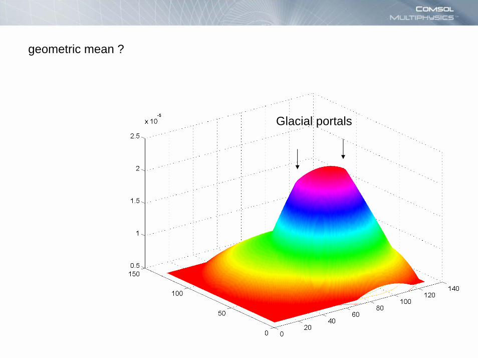
geometric mean ?

Glacial portals

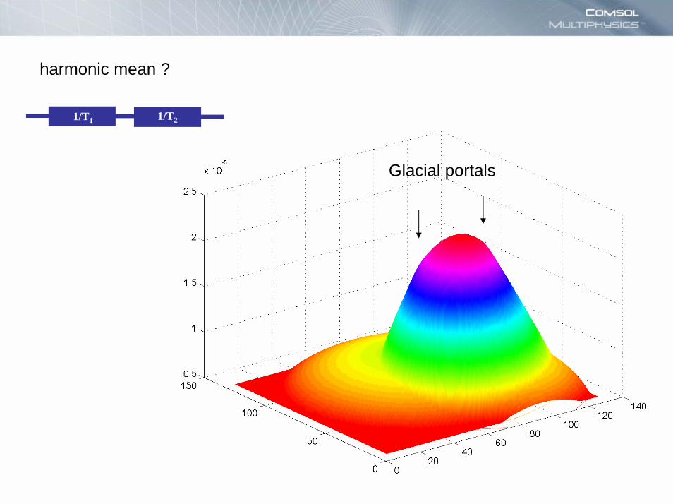
harmonic mean ?

1/T1 1/T2

Glacial portals

Difference in hydraulic conductivity betweenharmonic -and geometric mean

Hydraulic headInput: hydraulic head as arithmetic mean between the Trandum and Li deltas

arithmetic

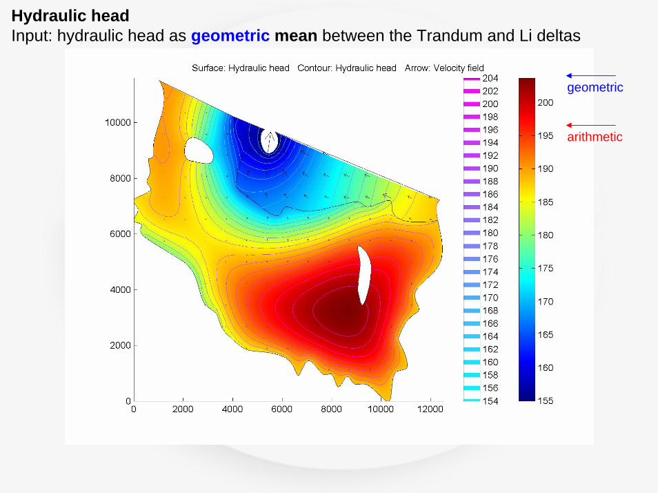
Hydraulic headInput: hydraulic head as geometric mean between the Trandum and Li deltas

arithmetic

geometric

Hydraulic headInput: hydraulic head as harmonic mean between the Trandum and Li deltas

arithmetic

geometric

harmonic

No terminal and railway culvert (drawdown)

Hydraulic head gradient,minimum gradient at ground water dividemax. gradient in ravine areas (landslide) and glacial boundary (kettle lake area)

With terminal and railway culvert (drawdown)

Hydraulic head gradient

To protect the preservation area, the water balance of the area has to be maintained because the hydraulic gradient is the driving force of the gully processes.

Hydraulic head gradientWith terminal and railway culvert (drawdown)and two injection points of water from the culvert

The Comsol meshing routines makes life more practical!

Plot cross-section before and after Airport construction

Note change in head gradient towards ravine area

The majority of the world population depends on groundwater resources

Groundwater resources of the worldImportant for society

Coastal aquifers: possible contamination of groundwater by seawater intrusion

Density driven flow:2-way coupling between flow & transport

• Density dependent fluid flow - Darcy’s Law expresses in terms of pressure p:

[ ] 0)(/])1([ =+∇−⋅∇+∂∂

∂∂

+∂∂

+− gDptc

ctp ρηκρρθζθθξρ

[ ] 0=+∇−⋅∇+∂∂ CcD

tc uθθ

• Salt concentration – Saturated solute transport

compressibility = 0

)( 0cc −+= γρρ• ρ varies with c

0ccs−=γ ρoρf −

where:

from the presentation byLeigh Soutter

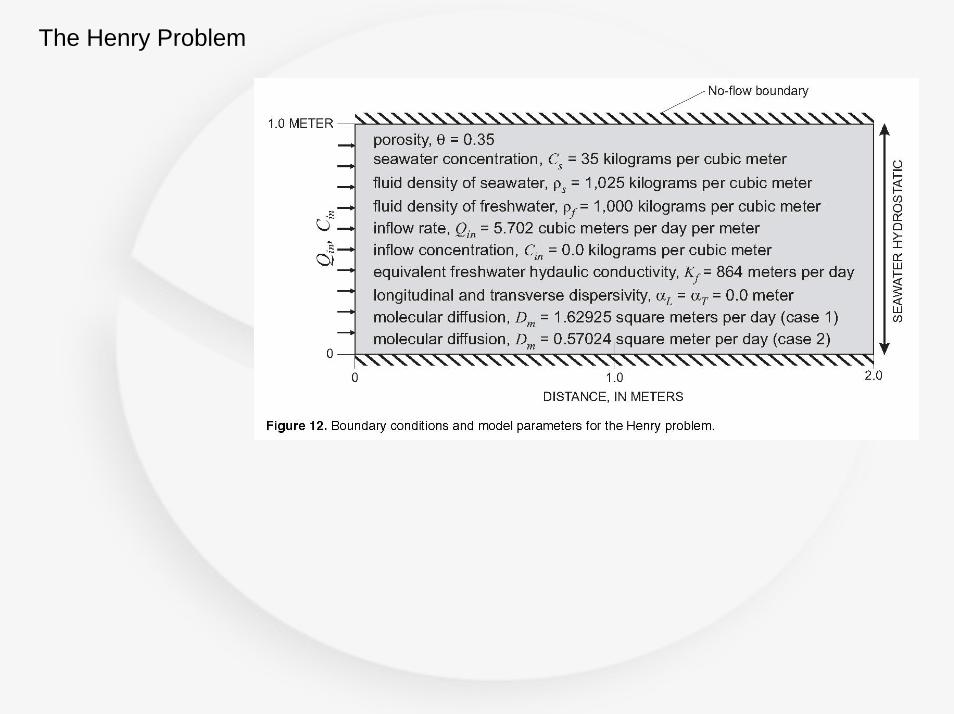
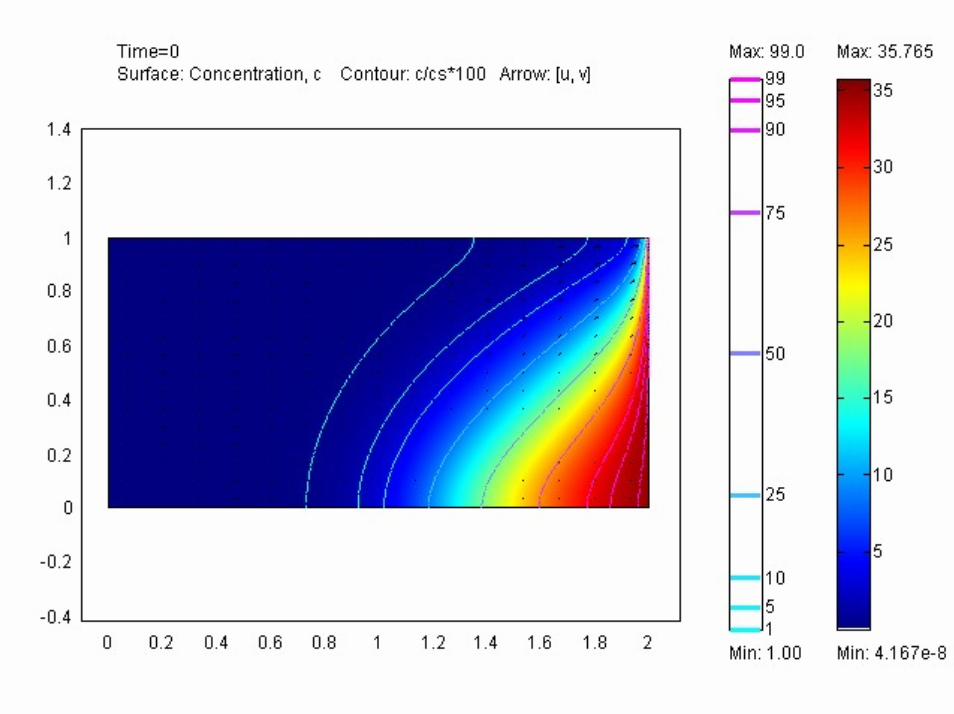
The Henry Problem

Dm = 1.6295 m2/d

Dm = 0.57024 m2/d

Decrease influx of fresh water from 5.702 m3/s to 0.05702 m3/s

Time variable boundary

conditions

What is the effect of tidal changes of 0.1 times thickness of aquifer?

and

it’s fun!

Conclusion

COMSOL MULTIPHYSICS is useful for

teachingand business

Thank you!