Embed Size (px)
Citation preview
New Variants of Variable Neighbourhood Search for 0-1
Mixed Integer Programming and Clustering
A thesis submitted for the degree of
Doctor of Philosophy
Jasmina Lazic
School of Information Systems, Computing and Mathematics
Brunel University
c©August 3, 2010
Contents
Contents i
List of Figures vi
List of Tables viii
List of Abbreviations ix
Acknowledgements xi
Related Publications xiii
Abstract 1
1 Introduction 3
1.1 Combinatorial Optimisation . . . . . . . . . . . . . . . . . . . . . . . . . . . . . . . 3
1.2 The 0-1 Mixed Integer Programming Problem . . . . . . . . . . . . . . . . . . . . . 11
1.3 Clustering . . . . . . . . . . . . . . . . . . . . . . . . . . . . . . . . . . . . . . . . . 17
1.4 Thesis Overview . . . . . . . . . . . . . . . . . . . . . . . . . . . . . . . . . . . . . 18
2 Local Search Methodologies in Discrete Optimisation 21
2.1 Basic Local Search . . . . . . . . . . . . . . . . . . . . . . . . . . . . . . . . . . . . 21
2.2 A Brief Overview of Local Search Based Metaheuristics . . . . . . . . . . . . . . . 24
2.2.1 Simulated Annealing . . . . . . . . . . . . . . . . . . . . . . . . . . . . . . . 24
2.2.2 Tabu Search . . . . . . . . . . . . . . . . . . . . . . . . . . . . . . . . . . . 26
2.2.3 Greedy Randomised Adaptive Search . . . . . . . . . . . . . . . . . . . . . 28
2.2.4 Guided Local Search . . . . . . . . . . . . . . . . . . . . . . . . . . . . . . . 29
2.2.5 Iterated Local Search . . . . . . . . . . . . . . . . . . . . . . . . . . . . . . 31
2.3 Variable Neighbourhood Search . . . . . . . . . . . . . . . . . . . . . . . . . . . . . 33
2.3.1 Basic Schemes . . . . . . . . . . . . . . . . . . . . . . . . . . . . . . . . . . 33
2.3.2 Advanced Schemes . . . . . . . . . . . . . . . . . . . . . . . . . . . . . . . . 40
2.3.3 Variable Neighbourhood Formulation Space Search . . . . . . . . . . . . . . 40
2.3.4 Primal-dual VNS . . . . . . . . . . . . . . . . . . . . . . . . . . . . . . . . . 41
2.3.5 Dynamic Selection of Parameters and/or Neighbourhood Structures . . . . 42
2.3.6 Very Large-scale VNS . . . . . . . . . . . . . . . . . . . . . . . . . . . . . . 43
i
ii Contents
2.3.7 Parallel VNS . . . . . . . . . . . . . . . . . . . . . . . . . . . . . . . . . . . 44
2.4 Local Search for 0-1 Mixed Integer Programming . . . . . . . . . . . . . . . . . . . 44
2.4.1 Local Branching . . . . . . . . . . . . . . . . . . . . . . . . . . . . . . . . . 47
2.4.2 Variable Neighbourhood Branching . . . . . . . . . . . . . . . . . . . . . . . 47
2.4.3 Relaxation Induced Neighbourhood Search . . . . . . . . . . . . . . . . . . 49
2.5 Future Trends: the Hyper-reactive Optimisation . . . . . . . . . . . . . . . . . . . 50
3 Variable Neighbourhood Search for Colour Image Quantisation 53
3.1 Related Work . . . . . . . . . . . . . . . . . . . . . . . . . . . . . . . . . . . . . . . 55
3.1.1 The Genetic C-Means Heuristic (GCMH) . . . . . . . . . . . . . . . . . . . 55
3.1.2 The Particle Swarm Optimisation (PSO) Heuristic . . . . . . . . . . . . . . 56
3.2 VNS Methods for the CIQ Problem . . . . . . . . . . . . . . . . . . . . . . . . . . . 57
3.3 Computational Results . . . . . . . . . . . . . . . . . . . . . . . . . . . . . . . . . . 59
3.4 Summary . . . . . . . . . . . . . . . . . . . . . . . . . . . . . . . . . . . . . . . . . 63
4 Variable Neighbourhood Decomposition Search for the 0-1 MIP Problem 67
4.1 The VNDS-MIP Algorithm . . . . . . . . . . . . . . . . . . . . . . . . . . . . . . . 68
4.2 Computational Results . . . . . . . . . . . . . . . . . . . . . . . . . . . . . . . . . . 70
4.3 Summary . . . . . . . . . . . . . . . . . . . . . . . . . . . . . . . . . . . . . . . . . 81
5 Applications of VNDS to Some Specific 0-1 MIP Problems 87
5.1 The Multidimensional Knapsack Problem . . . . . . . . . . . . . . . . . . . . . . . 87
5.1.1 Related Work . . . . . . . . . . . . . . . . . . . . . . . . . . . . . . . . . . . 89
5.1.2 VNDS-MIP with Pseudo-cuts . . . . . . . . . . . . . . . . . . . . . . . . . . 92
5.1.3 A Second Level of Decomposition in VNDS . . . . . . . . . . . . . . . . . . 96
5.1.4 Computational Results . . . . . . . . . . . . . . . . . . . . . . . . . . . . . . 98
5.1.5 Summary . . . . . . . . . . . . . . . . . . . . . . . . . . . . . . . . . . . . . 111
5.2 The Barge Container Ship Routing Problem . . . . . . . . . . . . . . . . . . . . . . 112
5.2.1 Formulation of the Problem . . . . . . . . . . . . . . . . . . . . . . . . . . . 112
5.2.2 Computational Results . . . . . . . . . . . . . . . . . . . . . . . . . . . . . . 118
5.2.3 Summary . . . . . . . . . . . . . . . . . . . . . . . . . . . . . . . . . . . . . 120
5.3 The Two-Stage Stochastic Mixed Integer Programming Problem . . . . . . . . . . 120
5.3.1 Existing Solution Methodology for the Mixed Integer 2SSP . . . . . . . . . 123
5.3.2 VNDS Heuristic for the 0-1 Mixed Integer 2SSP . . . . . . . . . . . . . . . 123
5.3.3 Computational Results . . . . . . . . . . . . . . . . . . . . . . . . . . . . . . 125
5.3.4 Summary . . . . . . . . . . . . . . . . . . . . . . . . . . . . . . . . . . . . . 127
6 Variable Neighbourhood Search and 0-1 MIP Feasibility 129
6.1 Related Work: Feasibility Pump . . . . . . . . . . . . . . . . . . . . . . . . . . . . 130
6.1.1 Basic Feasibility Pump . . . . . . . . . . . . . . . . . . . . . . . . . . . . . . 131
6.1.2 General Feasibility Pump . . . . . . . . . . . . . . . . . . . . . . . . . . . . 131
6.1.3 Objective Feasibility Pump . . . . . . . . . . . . . . . . . . . . . . . . . . . 132
6.1.4 Feasibility Pump and Local Branching . . . . . . . . . . . . . . . . . . . . . 133
6.2 Variable Neighbourhood Pump . . . . . . . . . . . . . . . . . . . . . . . . . . . . . 134
iii
6.3 Constructive Variable Neighbourhood Decomposition Search . . . . . . . . . . . . 136
6.4 Computational Results . . . . . . . . . . . . . . . . . . . . . . . . . . . . . . . . . . 136
6.5 Summary . . . . . . . . . . . . . . . . . . . . . . . . . . . . . . . . . . . . . . . . . 144
7 Conclusions 147
Bibliography 151
Index 171
A Computational Complexity 175
A.1 Decision Problems and Formal Languages . . . . . . . . . . . . . . . . . . . . . . . 175
A.2 Turing Machines . . . . . . . . . . . . . . . . . . . . . . . . . . . . . . . . . . . . . 176
A.3 Time Complexity Classes p and np . . . . . . . . . . . . . . . . . . . . . . . . . . . 180
A.4 np-Completeness . . . . . . . . . . . . . . . . . . . . . . . . . . . . . . . . . . . . . 181
B Statistical Tests 183
B.1 Friedman Test . . . . . . . . . . . . . . . . . . . . . . . . . . . . . . . . . . . . . . 183
B.2 Bonferroni-Dunn Test and Nemenyi Test . . . . . . . . . . . . . . . . . . . . . . . . 184
C Performance Profiles 185

iv Contents
List of Figures
1.1 Structural classification of hybridisations between metaheuristics and exact methods. 10
2.1 Basic local search. . . . . . . . . . . . . . . . . . . . . . . . . . . . . . . . . . . . . 22
2.2 Best improvement procedure. . . . . . . . . . . . . . . . . . . . . . . . . . . . . . . 23
2.3 First improvement procedure. . . . . . . . . . . . . . . . . . . . . . . . . . . . . . . 23
2.4 Local search: stalling in a local optimum. . . . . . . . . . . . . . . . . . . . . . . . 24
2.5 Simulated annealing. . . . . . . . . . . . . . . . . . . . . . . . . . . . . . . . . . . . 25
2.6 Geometric cooling scheme for Simulated annealing. . . . . . . . . . . . . . . . . . . 26
2.7 Tabu search. . . . . . . . . . . . . . . . . . . . . . . . . . . . . . . . . . . . . . . . 27
2.8 Greedy randomised adaptive search. . . . . . . . . . . . . . . . . . . . . . . . . . . 29
2.9 GLS: escaping from local minimum by increasing the objective function value. . . . 30
2.10 Guided local search. . . . . . . . . . . . . . . . . . . . . . . . . . . . . . . . . . . . 31
2.11 Iterated local search. . . . . . . . . . . . . . . . . . . . . . . . . . . . . . . . . . . . 32
2.12 The change of the used neighbourhood in some typical VNS solution trajectory. . . 34
2.13 VND pseudo-code. . . . . . . . . . . . . . . . . . . . . . . . . . . . . . . . . . . . . 35
2.14 RVNS pseudo-code. . . . . . . . . . . . . . . . . . . . . . . . . . . . . . . . . . . . 36
2.15 The basic VNS scheme. . . . . . . . . . . . . . . . . . . . . . . . . . . . . . . . . . 37
2.16 The Basic VNS pseudo-code. . . . . . . . . . . . . . . . . . . . . . . . . . . . . . . 37
2.17 General VNS. . . . . . . . . . . . . . . . . . . . . . . . . . . . . . . . . . . . . . . . 38
2.18 Skewed VNS. . . . . . . . . . . . . . . . . . . . . . . . . . . . . . . . . . . . . . . . 39
2.19 Variable neighbourhood decomposition search. . . . . . . . . . . . . . . . . . . . . 40
2.20 VNS formulation space search. . . . . . . . . . . . . . . . . . . . . . . . . . . . . . 41
2.21 Variable neighbourhood descent with memory. . . . . . . . . . . . . . . . . . . . . 42
2.22 Local search in the 0-1 MIP solution space. . . . . . . . . . . . . . . . . . . . . . . 46
2.23 Updating the neighbourhood size in LB. . . . . . . . . . . . . . . . . . . . . . . . . 47
2.24 Neighbourhood update in VND-MIP. . . . . . . . . . . . . . . . . . . . . . . . . . . 48
2.25 VNB shaking pseudo-code. . . . . . . . . . . . . . . . . . . . . . . . . . . . . . . . 48
2.26 Variable Neighbourhood Branching. . . . . . . . . . . . . . . . . . . . . . . . . . . 49
2.27 A standard local search-based metaheuristic. . . . . . . . . . . . . . . . . . . . . . 51
2.28 Hyper-reactive search. . . . . . . . . . . . . . . . . . . . . . . . . . . . . . . . . . . 52
2.29 The Hyper-reactive VNS. . . . . . . . . . . . . . . . . . . . . . . . . . . . . . . . . 52
3.1 RVNS for CIQ. . . . . . . . . . . . . . . . . . . . . . . . . . . . . . . . . . . . . . . 58
v
vi List of Figures
3.2 VNDS for CIQ. . . . . . . . . . . . . . . . . . . . . . . . . . . . . . . . . . . . . . . 59
3.3 Time performance of VNS quantisation methods . . . . . . . . . . . . . . . . . . . 62
3.4 MSE/running time comparison between the M-Median and the M-Means solution. 63
3.5 “Lenna” quantised to 16 colours: (a) M-Median solution, (b) M-Means solution. . 64
3.6 “Lenna” quantised to 64 colours: (a) M-Median solution, (b) M-Means solution. . 64
3.7 “Lenna” quantised to 256 colours: (a) M-Median solution, (b) M-Means solution. . 64
3.8 “Baboon” quantised to 16 colours: (a) M-Median solution, (b) M-Means solution. . 65
3.9 “Baboon” quantised to 64 colours: (a) M-Median solution, (b) M-Means solution. . 65
3.10 “Baboon” quantised to 256 colours: (a) M-Median solution, (b) M-Means solution. 65
3.11 “Peppers” quantised to 16 colours: (a) M-Median solution, (b) M-Means solution. 66
3.12 “Peppers” quantised to 64 colours: (a) M-Median solution, (b) M-Means solution. 66
3.13 “Peppers” quantised to 256 colours: (a) M-Median solution, (b) M-Means solution. 66
4.1 VNDS for MIPs. . . . . . . . . . . . . . . . . . . . . . . . . . . . . . . . . . . . . . 69
4.2 VND for MIPs. . . . . . . . . . . . . . . . . . . . . . . . . . . . . . . . . . . . . . . 70
4.3 Relative gap average over all instances in test bed vs. computational time. . . . . . 74
4.4 Relative gap average over demanding instances vs. computational time. . . . . . . 74
4.5 Relative gap average over non-demanding instances vs. computational time. . . . . 75
4.6 The change of relative gap with computational time for biella1 instance. . . . . . . 78
4.7 Relative gap values (in %) for large-spread instances. . . . . . . . . . . . . . . . . . 80
4.8 Relative gap values (in %) for medium-spread instances. . . . . . . . . . . . . . . . 80
4.9 Relative gap values (in %) for small-spread instances. . . . . . . . . . . . . . . . . 81
4.10 Relative gap values (in %) for very small-spread instances. . . . . . . . . . . . . . . 81
4.11 Bonferroni-Dunn critical difference from the solution quality rank of VNDS-MIP . 85
4.12 Bonferroni-Dunn critical difference from the running time rank of VNDS-MIP . . . 85
5.1 Linear programming based algorithm. . . . . . . . . . . . . . . . . . . . . . . . . . 89
5.2 An iterative relaxation based heuristic. . . . . . . . . . . . . . . . . . . . . . . . . . 91
5.3 An iterative independent relaxation based heuristic. . . . . . . . . . . . . . . . . . 92
5.4 VNDS-MIP with pseudo-cuts. . . . . . . . . . . . . . . . . . . . . . . . . . . . . . . 93
5.5 VNDS-MIP with upper and lower bounding and another ordering strategy. . . . . 96
5.6 Two levels of decomposition with hyperplanes ordering. . . . . . . . . . . . . . . . 97
5.7 Flexibility for changing the hyperplanes. . . . . . . . . . . . . . . . . . . . . . . . . 99
5.8 Performance profiles of all 7 algorithms over the OR library data set. . . . . . . . . 110
5.9 Performance profiles of all 7 algorithms over the GK data set. . . . . . . . . . . . . 111
5.10 Example itinerary of a barge container ship . . . . . . . . . . . . . . . . . . . . . . 114
5.11 VNDS-SIP pseudo-code. . . . . . . . . . . . . . . . . . . . . . . . . . . . . . . . . . 124
6.1 The basic feasibility pump. . . . . . . . . . . . . . . . . . . . . . . . . . . . . . . . 132
6.2 Constructive VND-MIP. . . . . . . . . . . . . . . . . . . . . . . . . . . . . . . . . . 135
6.3 The variable neighbourhood pump pseudo-code. . . . . . . . . . . . . . . . . . . . . 135
6.4 Constructive VNDS for 0-1 MIP feasibility. . . . . . . . . . . . . . . . . . . . . . . 139
List of Tables
3.1 The MSE of the VNS, GCMH and PSO heuristics . . . . . . . . . . . . . . . . . . 60
3.2 The MSE/CPU time of the RVNDS’, RVNDS, VNDS and RVNS algorithms . . . . 61
3.3 The MSE/CPU time comparison between the M-Median and M-Means solutions. . 62
4.1 Test bed information. . . . . . . . . . . . . . . . . . . . . . . . . . . . . . . . . . . 72
4.2 VNDS1 and VNDS2 time performance. . . . . . . . . . . . . . . . . . . . . . . . . 76
4.3 VNDS-MIP objective values for two different parameters settings . . . . . . . . . . 77
4.4 Objective function values for all the 5 methods tested. . . . . . . . . . . . . . . . . 78
4.5 Relative gap values (in %) for all the 5 methods tested. . . . . . . . . . . . . . . . 79
4.6 Running times (in seconds) for all the 5 methods tested. . . . . . . . . . . . . . . . 82
4.7 Algorithm rankings by the objective function values for all instances. . . . . . . . . 83
4.8 Algorithm rankings by the running time values for all instances. . . . . . . . . . . 84
4.9 Objective value average rank differences from VNDS-MIP . . . . . . . . . . . . . . 84
4.10 Running time average rank differences from VNDS-MIP . . . . . . . . . . . . . . . 84
5.1 Results for the 5.500 instances. . . . . . . . . . . . . . . . . . . . . . . . . . . . . . 102
5.2 Results for the 10.500 instances. . . . . . . . . . . . . . . . . . . . . . . . . . . . . 103
5.3 Results for the 30.500 instances. . . . . . . . . . . . . . . . . . . . . . . . . . . . . 104
5.4 Average results on the OR-Library. . . . . . . . . . . . . . . . . . . . . . . . . . . . 105
5.5 Extended results on the OR-Library. . . . . . . . . . . . . . . . . . . . . . . . . . . 106
5.6 Average results on the GK instances. . . . . . . . . . . . . . . . . . . . . . . . . . . 107
5.7 Comparison with other methods over the GK instances. . . . . . . . . . . . . . . . 108
5.8 Differences between the average solution quality ranks for all five methods. . . . . 109
5.9 Quality rank differences between the three one-level decomposition methods. . . . 110
5.10 The barge container ship routing test bed. . . . . . . . . . . . . . . . . . . . . . . . 118
5.11 Optimal values obtained by CPLEX/AMPL and corresponding execution times. . 119
5.12 Objective values (profit) and corresponding rankings for the four methods tested. . 120
5.13 Running times and corresponding rankings for the four methods tested. . . . . . . 121
5.14 Dimensions of the DCAP problems . . . . . . . . . . . . . . . . . . . . . . . . . . . 126
5.15 Test results for DCAP . . . . . . . . . . . . . . . . . . . . . . . . . . . . . . . . . . 126
5.16 Dimensions of the SIZES problems . . . . . . . . . . . . . . . . . . . . . . . . . . . 126
5.17 Test results for SIZES . . . . . . . . . . . . . . . . . . . . . . . . . . . . . . . . . . 127
5.18 Dimensions of the SSLP problems . . . . . . . . . . . . . . . . . . . . . . . . . . . 127
vii
viii List of Tables
5.19 Test results for SSLP . . . . . . . . . . . . . . . . . . . . . . . . . . . . . . . . . . . 128
6.1 Benchmark group I: instances from the MIPLIB 2003 library. . . . . . . . . . . . . 137
6.2 Benchmark group II: the additional set of instances from [103]. . . . . . . . . . . . 138
6.3 Solution quality results for instances from group I. . . . . . . . . . . . . . . . . . . 140
6.4 Solution quality results for instances from group II. . . . . . . . . . . . . . . . . . . 141
6.5 Computational time results for instances from group I. . . . . . . . . . . . . . . . . 142
6.6 Computational time results for instances from group II. . . . . . . . . . . . . . . . 143
6.7 Summarised results. . . . . . . . . . . . . . . . . . . . . . . . . . . . . . . . . . . . 144

List of Abbreviations
2SSP : two-stage stochastic problemB&B : branch-and-boundB&C : branch-and-cutCIQ : colour image quantizationFP : feasibility pumpGCMH : genetic C-Means heuristicGLS : guided local searchGRASP : greedy randomised adaptive searchILS : iterated local searchIRH : iterative relaxation based heuristicIIRH : iterative independent relaxation based heuristicLB : local branchingLP : linear programmingLPA : linear programming-based algorithmMIP : mixed integer programmingMIPs : mixed integer programming problemsMKP : multidimensional knapsack problemMP : mathematical programmingPD-VNS : primal-dual variable neighbourhood searchPSO : particle-swarm-optimisationRCL : restricted candidate listRINS : relaxation induced neighbourhood searchRS : reactive searchRVNS : reduced variable neighbourhood searchSA : simulated annealingTS : tabu searchVNB : variable neighbourhood branchingVND : variable neighbourhood descentVNDM : variable nighbourhood descent with memoryVND-MIP : variable neighbourhood descent for mixed integer programmingVNDS : variable neighbourhood decomposition searchVNDS-MIP : variable neighbourhood decomposition search for mixed integer programmingVNP : variable neighbourhood pumpVNS : variable neighbourhood search
ix

x List of Abbreviations
Acknowledgements
First of all, I would like to express my deep gratitude to my supervisor, Professor Dr NenadMladenovic, for introducing me to the fields of operations research and combinatorial optimisationand supporting my research over the years. I also want to thank Dr Mladenovic for providing mewith many research opportunities and introducing me to many internationally recognised scientists,which resulted in valuable collaborations and research work. His inspiration, competent guidanceand encouragement were of tremendous value for my scientific career.
Many thanks go to my second supervisor, Professor Dr Gautam Mitra, the head of theCARISMA research group, for his guidance and support. I would also like to thank the School ofInformation Systems, Computing and Mathematics (SISCM) at Brunel University for the extensivesupport during my PhD research years. My work was supported by a Scholarship and a Bursaryfunded by the SISCM at Brunel University.
Many special thanks go to the team at the LAMIH department, University of Valenciennesin France, for all the joint research which is reported in this thesis. I particularly want to thankProfessor Dr Said Hanafi for all his valuable corrections and suggestions. I also want to thankDr Christophe Wilbaut for providing the code of VNDS-HYP-FLE for comparison purposes (inChapter 5).
My thanks also go to the Mathematical Institute, Serbian Academy of Sciences and Arts,for supporting my PhD research at Brunel. I especially want to thank Dr Tatjana Davidovicfrom the Mathematical Institute and Vladimir Maras from the Faculty of Transport and TrafficEngineering at the University of Belgrade, for introducing me to the barge container ship routingproblem studied in Chapter 5 and providing the model presented in this thesis.
Many thanks again to Professor Gautam Mitra and Victor Zverovich from the SISCM atBrunel University, for collaborating with me on the two-stage stochastic mixed integer program-ming problem, included in Chapter 5 of this thesis.
I am also very grateful to Professor Dr Pierre Hansen from GERAD and HEC in Montreal,for his collaboration and guidance of my research work reported in Chapter 3 and for introducingme to the foundations of scientific research.
Finally, many thanks to my family and friends for bearing with me during these years.Special thanks go to Dr Matthias Maischak for all the definite and indefinite articles in this thesis.I also want to thank Matthias for his infinite love and support.
xi

xii Acknowledgements
Related Publications
• Published papers
◦ J. Lazic, S. Hanafi, N. Mladenovic and D. Urosevic. Variable Neighbourhood Decom-position Search for 0-1 Mixed Integer Programs. Computers and Operations Research,37 (6): 1055-1067, 2010.
◦ S. Hanafi, J. Lazic and N. Mladenovic. Variable Neighbourhood Pump Heuristic for 0-1Mixed Integer Programming Feasibility. Electronic Notes in Discrete Mathematics 36(C): 759–766, 2010, Elsevier.
◦ S. Hanafi, J. Lazic, N. Mladenovic, C. Wilbaut and I. Crevits. Hybrid Variable Neigh-bourhood Decomposition Search for 0-1 Mixed Integer Programming Problem. Elec-tronic Notes in Discrete Mathematics 36 (C): 883–890, 2010, Elsevier.
◦ J. Lazic, S. Hanafi, N. Mladenovic and D. Urosevic. Solving 0-1 Mixed Integer Programswith Variable Neighbourhood Decomposition Search. A Proceedings volume from the13th Information Control Problems in Manufacturing International Symposium, 2009.ISBN: 978-3-902661-43-2, DOI: 10.3182/20090603-3-RU-2001.0502
◦ S. Hanafi, J. Lazic, N. Mladenovic and C. Wilbaut. Variable Neighbourhood Decompo-sition Search with Bounding for Multidimensional Knapsack Problem. A Proceedingsvolume from the 13th Information Control Problems in Manufacturing InternationalSymposium, 2009. ISBN: 978-3-902661-43-2, DOI: 10.3182/20090603-3-RU-2001.0501
◦ P. Hansen, J. Lazic and N. Mladenovic. Variable neighbourhood search for colour imagequantization. IMA Journal of Management Mathematics 18 (2): 207-221, 2007.
• Papers submitted for publication
◦ S. Hanafi, J. Lazic, N. Mladenovic, C. Wilbaut and I. Crevits. Variable Neighbour-hood Decomposition Search with pseudo-cuts for Multidimensional Knapsack Problem.Submitted to Computers and Operations Research, special issue devoted to Multidi-mensional Knapsack Problem, 2010.
◦ S. Hanafi, J. Lazic, N. Mladenovic, C. Wilbaut and I. Crevits. Different Variable Neigh-bourhood Search Diving Strategies for Multidimensional Knapsack Problem. Submittedto Journal of Mathematical Modelling and Algorithms, 2010.
◦ T. Davidovic, J. Lazic, V. Maras and N. Mladenovic. MIP-based Heuristic Routing ofBarge Container Ships. Submitted to Transportation Science, 2010.
◦ J. Lazic, S. Hanafi and N. Mladenovic. Variable Neighbourhood Search Diving for 0-1MIP Feasibility. Submitted to Matheuristics 2010, the 3rd international workshop onmodel-based heuristics.
xiii

xiv Related Publications
◦ J. Lazic, G. Mitra, N. Mladenovic and V. Zverovich. Variable Neighbourhood Decom-position Search for a Two-stage Stochastic Mixed Integer Programming Problem. Sub-mitted to Matheuristics 2010, the 3rd international workshop on model-based heuristics.

Abstract
Many real-world optimisation problems are discrete in nature. Although recent rapid developmentsin computer technologies are steadily increasing the speed of computations, the size of an instanceof a hard discrete optimisation problem solvable in prescribed time does not increase linearly withthe computer speed. This calls for the development of new solution methodologies for solvinglarger instances in shorter time. Furthermore, large instances of discrete optimisation problemsare normally impossible to solve to optimality within a reasonable computational time/space andcan only be tackled with a heuristic approach.
In this thesis the development of so called matheuristics, the heuristics which are based onthe mathematical formulation of the problem, is studied and employed within the variable neigh-bourhood search framework. Some new variants of the variable neighbourhood search metaheuristicitself are suggested, which naturally emerge from exploiting the information from the mathemat-ical programming formulation of the problem. However, those variants may also be applied toproblems described by the combinatorial formulation. A unifying perspective on modern advancesin local search-based metaheuristics, a so called hyper-reactive approach, is also proposed. TwoNP-hard discrete optimisation problems are considered: 0-1 mixed integer programming and clus-tering with application to colour image quantisation. Several new heuristics for 0-1 mixed integerprogramming problem are developed, based on the principle of variable neighbourhood search. Oneset of proposed heuristics consists of improvement heuristics, which attempt to find high-qualitynear-optimal solutions starting from a given feasible solution. Another set consists of constructiveheuristics, which attempt to find initial feasible solutions for 0-1 mixed integer programs. Finally,some variable neighbourhood search based clustering techniques are applied for solving the colourimage quantisation problem. All new methods presented are compared to other algorithms rec-ommended in literature and a comprehensive performance analysis is provided. Computationalresults show that the methods proposed either outperform the existing state-of-the-art methodsfor the problems observed, or provide comparable results.
The theory and algorithms presented in this thesis indicate that hybridisation of the CPLEXMIP solver and the VNS metaheuristic can be very effective for solving large instances of the 0-1mixed integer programming problem. More generally, the results presented in this thesis sug-gest that hybridisation of exact (commercial) integer programming solvers and some metaheuristicmethods is of high interest and such combinations deserve further practical and theoretical in-vestigation. Results also show that VNS can be successfully applied to solving a colour imagequantisation problem.
1

2

Chapter 1
Introduction
1.1 Combinatorial Optimisation
Combinatorial optimisation, also known as discrete optimisation, is the field of applied mathe-matics which deals with solving combinatorial (or discrete) optimisation problems. Formally, anoptimisation problem P can be specified as finding
(1.1) ν(P ) = min{f(x) | x ∈ X, X ⊆ S}
where S denotes the solution space, X denotes the feasible region and f : S → R denotes theobjective function. If x ∈ X , we say that x is a feasible solution of the problem (1.1). Solutionx ∈ S is said to be infeasible if x /∈ X . Optimisation problem P is feasible if there is at least onefeasible solution of P . Otherwise, problem P is infeasible.
Formulation (1.1) assumes that the problem defined is a minimisation problem. A maximi-sation problem can be defined in the analogous way. However, it is obvious that any maximisationproblem can easily be reformulated as a minimisation one, by setting the objective function toF : S → R, with F (x) = −f(x), ∀x ∈ S, where f is the objective function of the originalmaximisation problem and S is the solution space.
If S = Rn, n ∈ N, problem (1.1) is called a continuous optimisation problem. Otherwise, if Sis finite, or infinite but enumerable, problem (1.1) is called combinatorial or discrete optimisationproblem. Although in some research literature combinatorial and discrete optimisation problemsare defined in different ways and do not necessarily represent the same type of problems (see,for instance, [33, 145]), in this thesis these two terms will be treated as synonymous and will beused interchangeably. Some special cases of combinatorial optimisation problems are the integeroptimisation problem when S = Zn, n ∈ N, the 0-1 optimisation problem when S = {0, 1}n, n ∈ N,and the mixed integer optimisation problem when S = Zn1×Rn2 , n1, n2 ∈ N. A particularly impor-tant special case of the combinatorial optimisation problem (1.1) is a mathematical programmingproblem, in which S ⊆ Rn and the feasible set X is defined as:
(1.2) X = {x | g(x) ≤ b},
where b ∈ Rm, g : Rn → Rm, g = (g1, g2, . . . , gm), gi : Rn → R, i ∈ {1, 2, . . . , m}, with gi(x) ≤ bi
being the ith constraint. If C is a set of constraints, the problem obtained by adding all constraintsin C to the mathematical programming problem P will be denoted as (P | C). In other words, ifP is an optimisation problem defined by (1.1), with feasible region X as in (1.2), then (P | C) is
3

4 Introduction
the problem of finding:
(1.3) min{f(x) | x ∈ X, x satisfies all constraints from C}.
An optimisation problem Q, defined with min{f(x) | x ∈ X, X ⊆ S}, is a relaxation of the
optimisation problem P , defined with (1.1), if and only if X ⊆ X and f(x) ≤ f(x) for all x ∈ X .If Q is a relaxation of P , then P is a restriction of Q. Relaxation and restriction for maximisationproblems are defined analogously.
Solution x∗ ∈ X of the problem (1.1) is said to be optimal, if
(1.4) f(x∗) ≤ f(x), ∀x ∈ X.
An optimal solution is also called optimum. In case of a minimisation problem, an optimal solutionis also called a minimal solution or simply a minimum. For a maximisation problem, the optimalitycondition (1.4) has the form: f(x∗) ≥ f(x), ∀x ∈ X . An optimal solution of a maximisationproblem is also called a maximal solution or a maximum. The optimal value ν(P ) of an optimisationproblem P defined by (1.1) is the objective function value f(x∗) of its optimal solution x∗ (theoptimal value of a minimisation/maximisation problem is also called the minimal/maximal value).Values l, u ∈ R are called a lower and an upper bound, respectively, for the optimal value ν(P ) ofthe problem P , if l ≤ ν(P ) ≤ u. Note that if Q is a relaxation of P (and P and Q are minimisationproblems), then the optimal value ν(Q) of Q is not greater than the optimal value ν(P ) of P . Inother words, the optimal value ν(Q) of problem Q is a lower bound for the optimal value ν(P ) ofP . Solving the problem (1.1) exactly means either finding an optimal solution x∗ ∈ X and provingthe optimality (1.4) of x∗, or proving that the problem has no feasible solutions, i.e. that X = ∅.
Many real-world (industrial, logistic, transportation, management, etc.) problems may bemodelled as combinatorial optimisation problems. They include various assignment and schedulingproblems, location problems, circuit and facility layout problems, set partitioning/covering, vehiclerouting, travelling salesman problem and many more. Therefore, a lot of research has been donein the development of efficient solution techniques in the field of discrete optimisation. In general,all combinatorial optimisation solution methods can be classified as either exact or approximate.An exact algorithm is the algorithm which solves an input problem exactly. Most commonly usedexact solution methods are branch-and-bound, dynamic programming, Lagrangian relaxation basedmethods, and linear programming based methods such as branch-and-cut, branch-and-price andbranch-and-cut-and-price. Some of them will be discussed in more details in Chapter 4 devoted to0-1 mixed integer programming. However, a great number of practical combinatorial optimisationproblem instances is proven to be np-hard [115], which means that they are not solvable by anypolynomial time algorithm (in terms of the size of the input instance), unless p = np holds1.Moreover, for the majority of problems which can be solved by a polynomial time algorithm, thepower of that polynomial may be so large that the solution cannot be obtained within a reasonabletimeframe. This is the reason why a lot of research has been carried out in designing efficientapproximate solution techniques for high complexity optimisation problems.
An approximate algorithm is an algorithm which does not necessarily provide an optimalsolution of an input problem, or the proof of infeasibility in case that the problem is infeasible.Approximate solution methods can be classified as either approximation algorithms or heuristics.An approximation algorithm is an algorithm which, for a given input instance P of an optimisationproblem (1.1), always returns a feasible solution x ∈ X of P (if one exists), such that the ratiof(x)/f(x∗), where x∗ is an optimal solution of the input instance P , is within a given approximationratio α ∈ R. More details on approximation algorithms can be found, for instance, in [47, 312].
1For more details on complexity classes p and np, the reader is referred to Appendix A.

Combinatorial Optimisation 5
Approximation algorithms can be viewed as methods which are guaranteed to provide solutions ofa certain quality. However, there is a number of np-hard optimisation problems which cannot beapproximated arbitrarily well (i.e. for which an efficient approximation algorithm does not exist),unless p = np [16]. In order to tackle these problems, one must employ methods which do notprovide any guarantees regarding either the solution quality, or the execution time limitations.Such methods are usually referred to as heuristic methods or simply heuristics. In [275], thefollowing definition of a heuristic is proposed: “A heuristic is a method which seeks good (i.e. near-optimal) solutions at a reasonable computational cost without being able to guarantee optimality,and possibly not feasibility. Unfortunately, it may not even be possible to state how close tooptimality a particular heuristic solution is.”. Since there is no guarantee regarding the solutionquality, a certain heuristic may have a very poor performance for some (bad) instances of a givenproblem. Nevertheless, a heuristic is usually considered good if it outperforms good approximationalgorithms on a majority of instances of a given problem. Moreover, a good heuristic may evenoutperform an exact algorithm regarding the computational time (i.e. usually provides a solutionof a better quality than the exact algorithm, if observed after a predefined execution time which isshorter than the total running time needed for the exact algorithm to provide an optimal solution).However, one should always bare in mind the so called No Free Lunch theorem (NFLT) [330], whichbasically states that there can be no optimisation algorithm which outperforms all the others onall problems. In other words, if an optimisation algorithm performs well on a particular sub classof problems, then the specific features of that algorithm, which exploit the characteristics of thatsub class, may prevent it from performing well on problems outside that class.
According to the general principle used for generating a solution of a problem, heuristicmethods can be classified as follows:
1) constructive methods
2) local search methods
3) inductive methods
4) problem decomposition/partitioning
5) methods that reduce the solution space
6) evolutionary methods
7) mathematical programming based methods
The heuristic types listed here are the most common ones. However, the concept of heuristicsallows for introducing new solution strategies, as well as combining the existing ones in differentways. Therefore, there is a number of other possible categories and it is hard (if possible) to makea complete classification of all heuristic methods. Comprehensive surveys on heuristic solutionmethods can be found, for instance, in [96, 199, 296, 336]. A brief description of each of theheuristic types stated above will be provided next. Some of these basic types will be discussed inmore details later in this thesis.
Constructive methods. Normally, only one (initial) feasible solution is generated. The solutionis constructed step by step, using the information from the problem structure. The two mostcommon approaches used are greedy and look-ahead. In a greedy approach (see [139] for example),the next solution candidate is always selected as the best candidate among the current set of pos-sible choices, according to some local criterion. At each iteration of a look-ahead approach, theconsequences of possible choices are estimated and solution candidates which can lead to a bad
6 Introduction
final solution are discarded (see [27] for example).
Local search methods. Local search methods, also known as improvement methods, start froma given feasible solution and gradually improve it in an iterative process, until a local optimum isreached. For each solution x, a neighbourhood of x is defined as a set of all feasible solutions whichare in a vicinity of x according to some predefined distance measure in the solution space of theproblem. At each iteration, a neighbourhood of the current candidate solution is explored and thecurrent solution is replaced with a better solution from its neighbourhood, if one exists. If thereare no better solutions in the observed neighbourhood, local optimum is reached and the solutionprocess terminates.
Inductive methods. The solution principles valid for small and simple problems are generalisedfor the larger and harder problems of the same type.
Problem decomposition/partitioning. The problem is decomposed into a number of smaller/simpler to solve subproblems and each of them is solved separately. The solution processes for thesubproblems can be either independent or intertwined in order to exchange the information aboutthe solutions of different subproblems.
Methods that reduce the solution space. Some parts of the feasible region are discardedfrom further consideration in such a way that the quality of the final solution is not significantlyaffected. Most common ways of reducing the feasible region include the tightening of the existingconstraints or introducing new constraints.
Evolutionary methods. As opposed to single-solution heuristics (sometimes also called trajec-tory heuristics), which only consider one solution at a time, evolutionary heuristics operate on apopulation of solutions. At each iteration, different solutions from the current population are com-bined, either implicitly or explicitly, to create new solutions which will form the next population.The general goal is to make each created population better than the previous one, according tosome predefined criterion.
Mathematical programming based methods. In this approach, a solution of a problem isgenerated by manipulating the mathematical programming (MP) formulation (1.1)-(1.2) of theproblem. The most common ways of manipulating the mathematical model are the aggregationof parameters, the modification of the objective function, and changing the nature of constraints(including modification, addition or deletion of particular constraints). A typical example of pa-rameter aggregation is the case of replacing a number of variables with a single variable, thusobtaining a much smaller problem. This small problem is then solved either exactly or approxi-mately, and the solution obtained is used to retrieve the solution of the original problem. Otherpossible ways of aggregation include aggregating a few stages of a multistage problem into a singlestage, or aggregating a few dimensions of a multidimensional problem into a single dimension. Awidely used modification of the objective function is Lagrangian relaxation [25], where one or moreconstraints, multiplied by Lagrange multipliers, are incorporated into the objective function (andremoved from the original formulation). This can also be viewed as an example of changing thenature of constraints. There are numerous other ways of manipulating the constraints within agiven mathematical model. One possibility is to weaken the original constraints by replacing sev-eral constraints with their linear combination [121]. Another is to discard several constraints andsolve the resulting model. The obtained solution, even if not feasible for the original problem, mayprovide some useful information for the solution process. Probably the most common approach

Combinatorial Optimisation 7
regarding the modification of constraints is the constraint relaxation, where a certain constraint isreplaced with one which defines a region containing the region defined by the original constraint. Atypical example is linear programming relaxation of integer optimisation problems, where integervariables are allowed to take real values.
The heuristic methods were first initiated in the late 1940s (see [262]). For several decades,only so called special heuristics were being designed. Special heuristics are heuristics which relyon the structure of the specific problem and therefore cannot be applied to other problems. In the1980s, a new approach for building heuristic methods has emerged. These more general solutionschemes, named metaheuristics [122], provide high level frameworks for building heuristics forbroader classes of problems. In [128], metaheuristics are described as “solution methods thatorchestrate an interaction between local improvement procedures and higher level strategies tocreate a process capable of escaping from local optima and performing a robust search of a solutionspace”. Some of the main concepts which can be distinguished in the development of metaheuristicsare the following:
1) diversification vs. intensification
2) randomisation
3) recombination
4) one vs. many neighbourhood structures
5) large neighbourhoods vs. small neighbourhoods
6) dynamic parameter adjustment
7) dynamic vs. static objective function
8) memory usage
9) hybridisation
10) parallelisation
Diversification vs. intensification. The term diversification refers to a shifting of the actualarea of search to a part of the search space which is far (with respect to some predefined dis-tance measure) from the current solution. In contrast, intensification refers to a more focusedexamination of the current search area, by exploiting all the information available from the searchexperience. Diversification and intensification are often referred to as exploration and exploitation,respectively. For a good metaheuristic, it is very important to find and keep an adequate balancebetween the diversification and intensification during the search process.
Randomisation. Randomisation allows the use of a random mechanism to select one or moresolutions from a set of candidate solutions. Therefore, it is closely related to the diversificationoperation discussed above and represents a very important element of most metaheuristics.
Recombination. The recombination operator is mainly associated with evolutionary metaheuris-tics (such as genetic algorithm [138, 243, 277]). It combines the attributes of two or more differentsolutions in order to form new (ideally better) solutions. In a more general sense, adaptive memory[123, 124, 301] and path relinking [133] strategies can be viewed as an implicit way of recombina-tion in single-solution metaheuristics.

8 Introduction
One vs. many neighbourhood structures. As mentioned previously, the concept of a neigh-bourhood plays a vital role in the construction of a local search method. However, most meta-heuristics employ local search methods in different ways. The way neighbourhood structures aredefined and explored may distinguish one metaheuristic from the other. Some metaheuristics,such as simulated annealing [4, 173, 196] or tabu search [131] for example (but also many others),work only with a single neighbourhood structure. Others, such as numerous variants of variableneighbourhood search (VNS) [159, 161, 163, 162, 164, 166, 167, 168, 237], operate on a set ofdifferent neighbourhood structures. Obviously, multiple neighbourhood structures usually providebetter means for both diversification and intensification. Consequently, it yields more flexibility inexploring the search space, which normally results in a higher overall efficiency of a metaheuris-tic. Although neighbourhood structures are usually not explicitly defined within an evolutionaryframework, one can observe that recombination and mutation (self-modification) operators definesolution neighbourhoods in an implicit way.
Large neighbourhoods vs. small neighbourhoods. As noted above, when designing a neigh-bourhood search type metaheuristic, a choice of neighbourhood structure, i.e. the way the neigh-bourhoods are defined, is essential for the efficiency and the effectiveness of the method. Normally,as the size of a neighbourhood increases, the higher is the quality of the local optima and the moreaccurate is the final solution. On the other hand, exploring large neighbourhoods is usually com-putationally extensive and demands longer execution times. Nevertheless, a number of methodswhich successfully deal with very large-scale neighbourhoods2 has been developed [10, 233, 235].They can be classified according to the techniques used to explore the neighbourhoods. In variabledepth methods, heuristics are used to explore the neighbourhoods [211]. Another group of methodsare those in which network flow or dynamic programming techniques are used for searching theneighbourhoods [64, 305]. Finally, there are methods in which large neighbourhoods are definedusing the restrictions of the original problem, so that they are solvable in polynomial time [135].
Dynamic parameter adjustment. It is convenient if a metaheuristic framework provides aform of an automatic parameter tuning, so that it is not necessary to perform extensive prelimi-nary experiments in order to adjust the parameters for each particular problem, when deriving aproblem-specific heuristic from a given metaheuristic. A number of so called reactive approaches,with an automatic (dynamic) parameter adjustment, has been proposed so far (see, for example,[22, 23, 44]).
Dynamic vs. static objective function. Whereas most metaheuristics deal with the sameobjective function during the whole solution process and use different diversification mechanismsin order to escape from local optima, there are some approaches which dynamically change theobjective function during the search, in that way changing the search landscape and avoiding thestalling in a local optimum. Some of the methods which use a dynamic objective function areguided local search [319] or reactive variable neighbourhood search [44].
Memory usage. The term memory (also referred to as search history) in a metaheuristic contextrefers to a storage of the relevant information during the search process (such as visited solutions,relevant solution properties, number of relevant iterations, etc.) and exploiting the collected in-formation in order to further guide the search process. Although it is explicitly used only in tabusearch [123, 131], there is a number of other metaheuristics which incorporate the memory usage inan implicit way. In genetic algorithm [277] and scatter search [133, 201], the population of solutions
2With the size usually exponential of the size of the input problem.
Combinatorial Optimisation 9
can be viewed as an implicit form of memory. The pheromone trails in Ant Colony Optimisation[88, 89] represent another example of implicit memory usage. In fact, a unifying approach forall metaheuristics with (implicit or explicit) memory usage was proposed in [301], called Adap-tive Memory Programming (AMP). According to AMP, each memory-based metaheuristic in someway memorises the information from a set of solutions and uses this information to construct newprovisional solutions during the search process. When combined with some other search method,AMP can be regarded as a higher-level metaheuristic itself, which uses the search history to guidethe subordinate method (see [123, 124]).
Hybridisation. Naturally, each metaheuristic has its own advantages and disadvantages in solvinga certain class of problems. This is why numerous hybrid schemes were designed, which combinethe algorithmic principles of several different metaheuristics [36, 265, 272, 302]. These hybridmethods usually outperform the original methods they were derived from (see, for example, [29]).
Parallelisation. Parallel implementations are aimed at further speed-up of the computationprocess and the improvement of solution space exploration. They are based on a simultaneoussearch space exploration by a number of concurrent threads, which may or may not communicateamong each other. Different parallel schemes may be derived depending on the subproblem/searchspace partition assigned to each thread and the communication scheme used. More theory onmetaheuristic parallelisation can be found in [70, 71, 72, 74].
For comprehensive reviews and bibliography on metaheuristic methods, the reader is referredto [37, 117, 128, 252, 253, 276, 282, 317]. For a given problem, it may be the case that oneheuristic is more efficient for a certain set of instances, whereas some other heuristic is moreefficient for another set of instances. Moreover, when solving one particular instance of a giveninput problem, it is possible that one heuristic is more efficient in one stage of the solution process,and some other heuristic in another stage. Lately, some new classes of higher-level heuristicmethods have emerged, such as hyper-heuristics [48], formulation space search [239, 240], variablespace search[175] or cooperative search [97]. A hyper-heuristic is a method which searches the spaceof heuristics in order to detect the heuristic method which is most efficient for a certain subsetof problem instances, or certain stages of the solution process for a given instance. As such, itcan be viewed as a response to limitations of optimisation algorithms imposed by the No FreeLunch theorem. The most important distinction between a hyper-heuristic and a heuristic for aparticular problem instance is that hyper-heuristic operates on the space comprised of heuristicmethods, rather than on the solution space of the original problem. Some metaheuristic methodscan also be utilised as hyper-heuristics. Formulation space search [239, 240] is based on the fact thata particular optimisation problem can often be formulated in different ways. As a consequence,different problem formulations induce different solution spaces. Formulation space search is ageneral framework for alternating between various problem formulations, i.e. switching betweenvarious solution spaces of the problem during the search process. The neighbourhood structuresand other search parameters are defined/adjusted separately for each solution space. The similaridea is exploited in the variable space search [175], where several search spaces for the graphcolouring problem are considered, with different neighborhood structures and objective functions.Like hyper-heuristics, cooperative search strategies also exploit the advantages of several heuristics[97]. However, cooperative search is usually associated with parallel algorithms (see, for instance,[177, 306]).
Another state of the art stream in the development of metaheuristics arises from a hybridi-sation of metaheuristics and mathematical programming (MP) techniques. The resulting hybridmethods are called matheuristics (short from math-heuristics). Since new solutions in the searchprocess are generated by manipulating the mathematical model of the input problem, matheuristics
10 Introduction
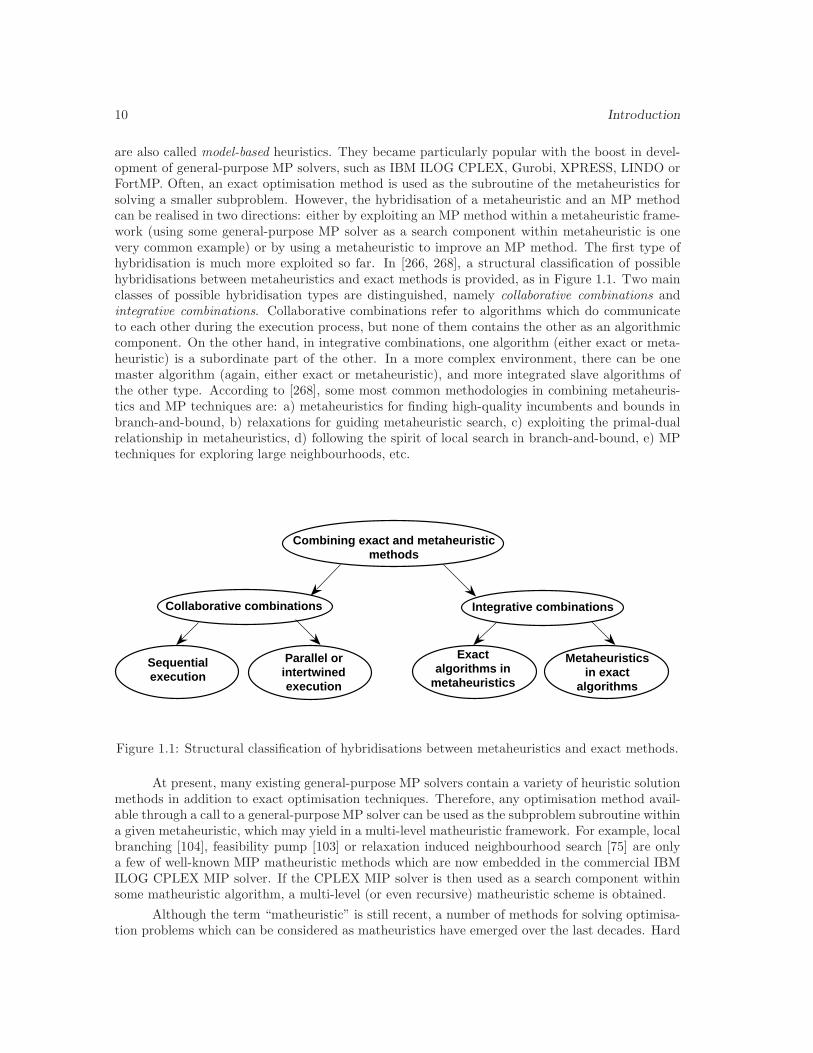
are also called model-based heuristics. They became particularly popular with the boost in devel-opment of general-purpose MP solvers, such as IBM ILOG CPLEX, Gurobi, XPRESS, LINDO orFortMP. Often, an exact optimisation method is used as the subroutine of the metaheuristics forsolving a smaller subproblem. However, the hybridisation of a metaheuristic and an MP methodcan be realised in two directions: either by exploiting an MP method within a metaheuristic frame-work (using some general-purpose MP solver as a search component within metaheuristic is onevery common example) or by using a metaheuristic to improve an MP method. The first type ofhybridisation is much more exploited so far. In [266, 268], a structural classification of possiblehybridisations between metaheuristics and exact methods is provided, as in Figure 1.1. Two mainclasses of possible hybridisation types are distinguished, namely collaborative combinations andintegrative combinations. Collaborative combinations refer to algorithms which do communicateto each other during the execution process, but none of them contains the other as an algorithmiccomponent. On the other hand, in integrative combinations, one algorithm (either exact or meta-heuristic) is a subordinate part of the other. In a more complex environment, there can be onemaster algorithm (again, either exact or metaheuristic), and more integrated slave algorithms ofthe other type. According to [268], some most common methodologies in combining metaheuris-tics and MP techniques are: a) metaheuristics for finding high-quality incumbents and bounds inbranch-and-bound, b) relaxations for guiding metaheuristic search, c) exploiting the primal-dualrelationship in metaheuristics, d) following the spirit of local search in branch-and-bound, e) MPtechniques for exploring large neighbourhoods, etc.
Combining exact and metaheuristicmethods
Collaborative combinations Integrative combinations
Sequentialexecution
Parallel orintertwinedexecution
Exactalgorithms in
metaheuristics
Metaheuristicsin exact
algorithms
Figure 1.1: Structural classification of hybridisations between metaheuristics and exact methods.
At present, many existing general-purpose MP solvers contain a variety of heuristic solutionmethods in addition to exact optimisation techniques. Therefore, any optimisation method avail-able through a call to a general-purpose MP solver can be used as the subproblem subroutine withina given metaheuristic, which may yield in a multi-level matheuristic framework. For example, localbranching [104], feasibility pump [103] or relaxation induced neighbourhood search [75] are onlya few of well-known MIP matheuristic methods which are now embedded in the commercial IBMILOG CPLEX MIP solver. If the CPLEX MIP solver is then used as a search component withinsome matheuristic algorithm, a multi-level (or even recursive) matheuristic scheme is obtained.
Although the term “matheuristic” is still recent, a number of methods for solving optimisa-tion problems which can be considered as matheuristics have emerged over the last decades. Hard
The 0-1 Mixed Integer Programming Problem 11
variable fixing (i.e. setting some variables to particular values) to generate smaller subproblems,easier to solve than the original problem, is probably one of the oldest approaches in a matheuris-tic design. One of the first methods which employs this principle is a convergent algorithm forpure 0-1 integer programming proposed in [298]. It solves a series of small subproblems gener-ated by exploiting information obtained by exactly solving a series of linear programming (LP)relaxations. Several enhanced versions of this algorithm have been proposed (see [154, 326]). In[268, 269], methods of this type are also referred to as core methods. Usually, an LP relaxationof the original problem is used to guide the fixation process. In general, exploiting the pieces ofinformation contained in the solution of the LP relaxation can be a very powerful tool for tacklingMP problems. In [57, 271], the solutions of the LP relaxation and its dual were used to conductthe mutation and recombination process in hybrid genetic algorithms for the multi-constrainedknapsack problem. Local search based metaheuristics proved to be very effective when combinedwith exact optimisation techniques, since it is usually convenient to search the neighbourhoodsby means of some exact algorithm. Large neighbourhood search (LNS) introduced in [294], verylarge-scale neighbourhood search in [10], or dynasearch [64] are some well-known matheuristic ex-amples of this type. In [155, 156], the dual relaxation solution is used within VNS in order tosystematically tighten the bounds during the solution process. The resulting primal-dual variableneighbourhood search methods were successful in solving the simple plant location problem [155]and large p-median clustering problems [156]. With the rapid development of the commercial MPsolvers, the use of a generic ready-made MP solver as a black-box search component is becom-ing increasingly popular. Some existing neighbourhood search type matheuristics which exploitgeneric MIP solvers for neighbourhood search are local branching (LB) [104] and VNS branching[169]. Another popular approach in matheuristics development is improving the performance ofthe branch-and-bound (B&B) algorithm by means of some metaheuristic methods. The genetic al-gorithm was successfully incorporated within a B&B search in [198] for example. Guided dives andrelaxation induced neighbourhood search (RINS), proposed in [75], explore some neighbourhood ofthe incumbent integer solution in order to choose the next node to be processed in the B&B tree.In [124], an adaptive memory projection (AMP) method for pure and mixed integer programmingwas proposed, which combines the principle of projection techniques with the adaptive memoryprocesses of tabu search to set some explicit or implicit variables to some particular values. Thisphilosophy can be used for unifying and extending a number of other procedures: LNS [294], localbranching [104], the relaxation induced neighbourhood search [75], VNS branching [169], or theglobal tabu search intensification using dynamic programming (TS-DP) [327]. For more detailson matheuristic methods the reader is referred to [40, 219, 266, 268].
1.2 The 0-1 Mixed Integer Programming Problem
The linear programming (LP) problem consists of minimising or maximising a linear function,subject to some equality or inequality linear constraints.
(1.5) (LP)
min∑n
j=1 cjxj
s.t.∑n
j=1 aijxj ≥ bi i = 1..m
xj ≥ 0 j = 1..n
Obviously, the LP problem (1.5) is a special case of an optimisation problem (1.1) and, morespecifically, of a mathematical programming problem, where all functions gi : Rn → R, i ∈{1, 2, . . . , m}, from (1.2) are linear. When all variables in the LP problem (1.5) are required to beinteger, the resulting optimisation problem is called a (pure) integer linear programming problem.If only some of the variables are required to be integer, the resulting problem is called a mixed

12 Introduction
integer linear programming problem, or simply a mixed integer programming problem. In furthertext, any linear programming problem in which the set of integer variables is non-empty will bereferred to as a mixed integer programming (MIP) problem. Furthermore, if some of the variablesin a MIP problem are required to be binary (i.e. either 0 or 1), the resulting problem is called a0-1 MIP problem. In general, a 0-1 MIP problem can be expressed as:
(1.6) (0− 1 MIP)
min∑n
j=1 cjxj
s.t.∑n
j=1 aijxj ≥ bi ∀i ∈M = {1, 2, . . . , m}xj ∈ {0, 1} ∀j ∈ B 6= ∅xj ∈ Z+
0 ∀j ∈ G,G ∩ B = ∅xj ≥ 0 ∀j ∈ C, C ∩ G = ∅, C ∩ B = ∅
where the set of indices N = {1, 2, . . . , n} of variables is partitioned into three subsets B,G and Cof binary, general integer and continuous variables, respectively, and Z+
0 = {x ∈ Z | x ≥ 0}. If theset of general integer variables in a 0-1 MIP problem is empty, the resulting 0-1 MIP problem isreferred to as a pure 0-1 MIP. Furthermore, if all variables in a pure 0-1 MIP are required to beinteger, the resulting problem is called pure 0-1 integer programming problem.
If P is a given 0-1 MIP problem, a linear programming relaxation LP(P ) of problem P isobtained by dropping all integer requirements on the variables from P :
(1.7) LP(0− 1 MIP)
min∑n
j=1 cjxj
s.t.∑n
j=1 aijxj ≥ bi ∀i ∈M = {1, 2, . . . , m}xj ∈ [0, 1] ∀j ∈ B 6= ∅xj ≥ 0 ∀j ∈ C ∪ G
The theory of linear programming as a maximisation/minimisation of a linear function sub-ject to some linear constraints was first conceived in the 1940s. At that time, mathematiciansGeorge Dantzig and George Stigler were independently working on different problems, both nowa-days known to be the problems of linear programming. George Dantzig was engaged with thedifferent planning, scheduling and logistical supply problems for the USA Air Force. As a result,in 1947 he formulated the planning problem with the linear objective function subject to satisfyinga system of linear equalities/inequalities, thus formalising the concept of a linear programmingproblem. He also proposed the simplex solution method for the linear programming problems [76].Note that the term “programming” is not related to computer programming, as one could assume,but rather to the planning of military operations (deployment, logistics, etc.), as used in militaryterminology. At the same time, George Stigler was working on the problem of the minimal cost ofsubsistence. He formulated a diet problem — achieving the minimal subsistence cost by fulfillinga number of nutritional requirements — as a linear programming problem [299]. For more detailson the historical development of linear programming, the reader is referred to [79, 290].
Numerous combinatorial optimisation problems, including a wide range of practical prob-lems in business, engineering and science can be modelled as 0-1 MIP problems (see [331]). Severalspecial cases of the 0-1 MIP problem, such as knapsack, set packing, network design, proteinalignment, travelling salesman and some other routing problems, are known to be np-hard [115].Complexity results prove that the computational resources required to optimally solve some 0-1MIP problem instances can grow exponentially with the size of the problem instance. Over severaldecades many contributions have led to successive improvements in exact methods such as branch-and-bound, cutting planes, branch-and-cut, branch-and-price, dynamic programming, Lagrangianrelaxation and linear programming. For a more detailed review on exact MIP solution methods,the reader is referred to [223, 331], for example. However, many MIP problems still cannot be
The 0-1 Mixed Integer Programming Problem 13
solved within acceptable time and/or space limits by the best current exact methods. As a con-sequence, metaheuristics have attracted attention as possible alternatives or supplements to themore classical approaches.
Branch-and-Bound. Branch-and-bound (B&B) (see, for instance, [118, 204, 236, 331]) is proba-bly the most commonly used solution technique for MIPs. The basic idea of B&B is the “divideand conquer” philosophy. The original problem is divided into smaller subproblems (also calledcandidate problems), which are again divided into even smaller subproblems and so on, as long asthe obtained subproblems are not easy enough to be solved.
More formally, if the original MIP problem P is given in the form minx∈X ctx (i.e. the feasibleregion of P is the set X), then the following candidate problems are created: Pi = minx∈Xi
ctx, i =1, 2, . . . , k, Xi ⊆ X, ∀i ∈ {1, 2, . . . , k}. Ideally, the feasible sets of the candidate problems should
be collectively exhaustive:⋃k
i=1 Xi = X , so that the optimal solution of P is the optimal solutionof at least one of the subproblems Pi, i ∈ {1, 2, . . . , k}. Also, it is desirable that the feasible setsof the candidate problems are mutually exclusive, i.e. Xi ∩Xj = ∅, for i 6= j, so that no area ofsolution space is explored more than once. Note that the original problem P is a relaxation of thecandidate problems P1, P2, . . . , Pk.
In a B&B solution process, a candidate problem is selected from the candidate list (the cur-rent list of candidate problems of interest) and, depending on its properties, the problem consideredis either removed from the candidate list, or used as a parent problem to create new candidateproblems to be added to the list. The process of removing a candidate problem from the candidatelist is called fathoming. Normally, candidate problems are not solved directly, but some relaxationsof candidate problems are solved instead. The relaxation to be used should be selected in sucha way that it is easy to solve and tight. A relaxation of an optimisation problem P is said to betight, if its optimal value is very close (or equal) to the optimal value of P . Most often, the LPrelaxation is used for this purpose [203]. However, the use of other relaxations is also possible.Apart from the LP relaxation, a so called Lagrangian relaxation [171, 172, 223] is probably mostwidely used.
Let Pi be the current candidate problem considered and x∗ the incumbent best solution ofP found so far. The optimal value ν(LP(Pi)) of the LP relaxation LP(Pi) is a lower bound of theoptimal value ν(Pi) of Pi. The following possibilities can be distinguished:
Case 1 There are no feasible solutions for the relaxed problem LP(Pi). This means that theproblem Pi itself is infeasible and does not need to be considered further. Hence, Pi can beremoved from the candidate list.
Case 2 The solution of LP(Pi) is feasible for P . If ν(LP(Pi)) is less then the incumbent best valuezUB = ctx∗, the solution of LP(Pi) becomes the new incumbent x∗. The candidate problemPi can be dropped from further consideration and removed from the candidate list.
Case 3 The optimal value ν(LP(Pi) of LP(Pi) is greater than the incumbent best value zUB =ctx∗. Since ν(LP(Pi)) ≤ ν(Pi), this means that also ν(Pi) > ctx∗ and Pi can be removedfrom the candidate list.
Case 4 The optimal value ν(LP(Pi)) of LP(Pi) is less than the incumbent best value zUB = ctx∗,but the solution of LP(Pi) is not feasible for P . In this case, there is a possibility that theoptimal solution of Pi is better than x∗, so the problem Pi needs to be further considered.Thus, Pi is added to the candidate list.
The difference between the optimal value ν(P ) of a given MIP problem P and the optimalvalue ν(LP(P )) of its LP relaxation LP(P ) is called the integrality gap. An important issue for the
14 Introduction
performance of B&B is the candidate problems selection strategy. In practice, the efficiency of aB&B method is greatly influenced by the integrality gap values of the candidate problems. A largeintegrality gap may lead to a very large candidate list, causing B&B to be very computationallyexpensive. A common candidate problem selection strategy is to choose the problem with thesmallest optimal value of the LP relaxation.
The steps of the B&B method for a given MIP problem P can be presented as below:
1) Initialisation. Set the incumbent best upper bound zUB to infinity: zUB = +∞. Solve theLP relaxation LP(P ) of P . If LP(P ) is infeasible, then P is infeasible as well. If the solutionx of LP(P ) is feasible for P , return x as an optimal solution of P . Otherwise, add LP(P ) tothe list of candidate problems and go to 2.
2) Problem selection. Select a candidate problem Pcandidate from the list of candidate problemsand go to 3.
3) Branching. The current candidate problem Pcandidate has at least one fractional variable xi,with i ∈ B ∪ G.
a) Select a fractional variable xi = ni + fi, i ∈ B ∪ G, ni ∈ Z, fi ∈ (0, 1), for the purposeof branching.
b) Create two new candidate problems (P | xi ≥ ni + 1) and (P | xi ≤ ni) (recall (1.3)).
c) For each of the two new candidate problems created, solve the LP relaxation of theproblem and update the candidate list according to cases 1-4 above.
4) Optimality test. Remove from the candidate list all candidate problems Pj with ν(LP(Pj)) ≥zUB. If the candidate list is empty, then the original input problem is either infeasible (incase zUB = +∞) or has the optimal solution zUB, and algorithm stops. Otherwise, go to 2.
Different variants of B&B can be obtained by choosing different strategies for candidateproblem selection (step 2 in the above algorithm), the branching variable selection (step 3a))and creating more then two candidate problems in each branching step. For more details onsome advanced B&B developments, the reader is referred to [223, 331], for example. From thepurely theoretical point of view, B&B will always find an optimal solution, if one exists. However,in practice, available computational resources will not allow B&B to find an optimum within areasonable time/space. This is why alternative MIP solution methods are sought.
Cutting Planes. The use of cutting planes for MIP was first proposed by Gomory in the late1950s [140, 141]. The basic idea of the cutting planes method for a given MIP problem P is toadd constraints to the problem during the search process, and thus produce relaxations which aretighter than the standard LP relaxation LP(P ). In other words, the added constraints shoulddiscard those areas of the feasible region of the LP relaxation LP(P ), which do not contain anypoints with imposed integrality constraints in the original MIP problem P .
More formally, if X = {x ∈ Rn | xj ∈ {0, 1}, j ∈ B, xj ∈ N ∪ {0}, j ∈ G, xj ≥ 0, j ∈ C} is thefeasible region of a MIP problem P , where B ∪ G 6= ∅,B ∪ G ∪ C = {1, 2, . . . , n}, then the convexhull of X is defined by:
(1.8) conv(X) = {λ1x1 + λ2x2 + . . . + λnxn |n∑
i=1
λi = 1, λi ≥ 0 for all i ∈ {1, 2, . . . , n}}
and the feasible region of LP(P ) is defined by
(1.9) X = {x ∈ Rn | xj ∈ [0, 1], j ∈ B, xj ≥ 0, j ∈ G ∪ C,B ∪ G 6= ∅}.
The 0-1 Mixed Integer Programming Problem 15
The idea is to add a constraint/set of constraints C to the problem P , so that the feasible regionX ′ of the problem (P | C) is between conv(X) and X [223], i.e.: conv(X) ⊆ X ′ ⊆ X .
Definition 1.1 Let X ⊆ Rn, n ∈ N. A valid inequality of X is an inequality (α)tx ≤ β, suchthat (α)tx ≤ β holds for all x ∈ X. A valid inequality is also called a cutting plane or a cut.
According to the mixed integer finite basis theorem (see [223], for example), if X is thefeasible region of a MIP problem, then the convex hull conv(X) of X is a polyhedron, i.e. canbe represented in the form conv(X) = {x ∈ Rn | (αi)tx ≤ βi, i = 1, 2, . . . , q, αi ∈ Rn, βi ∈ R}.Cutting planes added to the original MIP problem during the search process should ideally formthe subset of the system of inequalities (αi)tx ≤ βi, i = 1, 2, . . . , q which define conv(X).
Given a system of equalities∑n
j=1 aijxj = bi, i = 1, 2, . . . , m, an aggregate constraint
(1.10)
n∑
j=1
(m∑
i=1
uiaij
)xj =
m∑
i=1
uibi
can be generated by multiplying the original system of equalities by each of the given multipliersui, i = 1, 2, . . . , m and summing up the resulting systems of equalities. In a MIP case, all thevariables are required to be nonnegative, so a valid cut is obtained by rounding the aggregateconstraint (1.10):
(1.11)
n∑
j=1
⌊(m∑
i=1
uiaij
)⌋xj ≤
m∑
i=1
uibi
In a pure integer case, when all variables in the original MIP problem are required to be integer,the right-hand side of the cut (1.11) can be further rounded down, yielding:
(1.12)
n∑
j=1
⌊(m∑
i=1
uiaij
)⌋xj ≤
⌊m∑
i=1
uibi
⌋.
The cutting plane (1.12) is called a Chavatal-Gomory (C-G) cut [223]. In a pure integer case, theC-G cut is normally generated starting from the solution x of the LP relaxation LP(P ) of theoriginal MIP problem P . For more theory on C-G cuts and the procedures for deriving C-G cuts,the reader is referred to [52, 140, 141].
At the time when it was proposed, the cutting plane method was not effective enough. Themain drawbacks were a significant increase in the number of non-zero coefficients and roundoffproblems with the cuts used, resulting in a very slow convergence. In addition, an extension to amixed integer case (when not all of the variables are required to be integer) is not straightforward,since the inequality (1.11) does not imply the inequality (1.12) if some of the variables xj , j =1, 2, . . . , n are allowed to be continuous. For these reasons, the cutting plane methods were notpopular for a long time after they were first introduced. They regained popularity in the 1980s,when the development of the polyhedral theory led to the design of more efficient cutting planes[73]. Additional resources on the cutting planes theory can be found in [223, 331], for example.It appears that the use of cutting planes is particularly effective when combined with the B&Bmethod, which is discussed in the next subsection.
Branch-and-Cut. The branch-and-cut method (B&C) combines the B&B and cutting planesMIP solution methods, with the aim to bring together the advantages of both (see, for instance,[223]). Indeed, it seems promising to first tighten the problem by adding cuts and thus reduce the

16 Introduction
amount of enumeration to be performed by B&B. Furthermore, adding cuts before performing thebranching can be very effective in reducing the integrality gap [73]. The basic steps of the B&Cmethod for a given MIP problem P can be represented as below:
1) Initialisation. Set the incumbent best upper bound zUB to infinity: zUB = +∞. Set thelower bound zLB to infinity: zLB = −∞. Initialise the list of candidate problems: L = ∅.
2) LP relaxation. Solve the LP relaxation LP(P ) of P . If LP(P ) is infeasible or ν(LP(P )) >zUB, then go to step 4. Update the lower bound zLB = min{zLB, ν(LP(P ))}. If the solutionx of LP(P ) is feasible for P , return x as an optimal solution of P . Otherwise, replace thelast added problem in L with LP(P ) (or simply add LP(P ) to L if L = ∅) and go to 3.
3) Add cuts. Add cuts to P and go to step 2.
4) Problem selection. If L = ∅ go to 6. Otherwise, select a candidate problem Pcandidate ∈ Land go to 5.
5) Branching. The current candidate problem Pcandidate has at least one fractional variable xi,with i ∈ B∪G. Select a variable xi for the branching purposes, and branch on xi as in B&B.Go to step 6.
6) Optimality test. Remove from the candidate list all candidate problems Pj with ν(LP(Pj)) ≥zUB. If the candidate list is emptied, then the original input problem is either infeasible (incase zUB = +∞) or has the optimal solution zUB, and algorithm stops. Otherwise, go to 4.
The above algorithm is a simple variant of B&C, in which cutting planes are only addedbefore the initial branching is performed, i.e. only at the root node of a B&B tree. In moresophisticated variants of B&C, cutting planes are added at each node of the B&B tree, i.e. to eachof the candidate problems produced in step 5) above. In that case, it is important that each cutadded at a certain node of a B&B tree is also valid at all other nodes of that B&B tree. Also, ifcutting planes are added at more than one node of a B&B tree, the value of the lower bound zLB
is used to update the candidate list in the branching step (step 5) in the algorithm above).
B&C is nowadays a standard component in almost all generic MIP solvers. It is oftenused in conjunction with various heuristics for determining the initial upper bound at each node.For more details on the theory and performance of B&C, the reader is referred to, for example,[17, 67, 91, 142, 223].
Branch-and-Price. In the column generation approach (see, for example [85]), a small subset ofvariables is selected and the corresponding restricted LP relaxation is solved. The term “columngeneration” comes from the fact that selected variables actually represent columns in matrix nota-tion of the original MIP problem. Then variables which are not yet included are evaluated in orderto include those which lead to the best improvement of the current solution. This subproblemis called a pricing problem. After adding a new variable, the process is iterated until there areno more variables to add. The column generation approach can be viewed as a dual approach tocutting planes, because the variables in the primal LP problem correspond to the inequalities inthe dual LP problem. Branch-and-price method is obtained if column generation is performed ateach node of the branch-and-bound tree.
Heuristics for 0-1 Mixed Integer Programming. Although exact methods can successfullysolve to optimality problems with small dimensions (see, for instance, [298]), for large-scale prob-lems they cannot find an optimal solution with reasonable computational effort, hence the need tofind near-optimal solutions.

Clustering 17
The 0-1 MIP solution space is especially convenient for the local search based exploration.Some successful applications of tabu search for 0-1 MIPs can be found in [213, 147], for example.An application of simulated annealing for a special case of 0-1 MIP problem was proposed in [195].A number of other approaches for tackling MIPs has been proposed over the years. Examples ofpivoting heuristics, which are specifically designed to detect MIP feasible solutions, can be foundin [19, 20, 94, 214]. For more details about heuristics for 0-1 MIP feasibility, including more recentapproaches such as feasibility pump [103], the reader is referred to Chapter 6. Some other localsearch approaches for 0-1 MIPs can be found in [18, 129, 130, 176, 182, 212]. More recently, somehybridisatons with general-purpose MIP solvers have arisen, where either local search methods areintegrated as node heuristics in the B&B tree within a solver [32, 75, 120], or high-level heuristicsemploy a MIP solver as a black-box local search tool [103, 105, 106, 104, 169]. For more details onlocal search in the 0-1 MIP solution space, the reader is referred to Chapter 2.
Population based heuristics can also be successfully employed for tackling the 0-1 MIPproblem. Scatter search [132, 133] for 0-1 MIPs was proposed in [134]. Some applications ofgenetic algorithms include [39, 194, 216, 225]. In [284], an evolutionary algorithm was integratedwithin a B&B search tree. Some other interesting applications of evolutionary algorithms for mixedinteger programming can be found in [55, 335].
1.3 Clustering
Clustering is a process of partitioning a given set of objects into a number of different cate-gories/groups/subsets, which are referred to as clusters. The partitioning should be done in such away that objects belonging to the same cluster are similar (according to some predefined criteria),whereas objects which are not in the same cluster should be different (the criteria for measuring thelevel of difference does not necessarily need to be the same as the criteria for measuring the levelof similarity). For detailed listings of possible similarity and dissimilarity measures, the reader isreferred to [157, 333].
The two most commonly studied types of clustering are hierarchical clustering and par-titional clustering. Consider a set E = {x1, . . . , xN}, xj = (x1j , . . . , xqj), of N entities (orpoints) in Euclidean space Rq. Then the task of partitional clustering is to find a partitionPM = {C1, C2, . . . , CM} of E into M clusters, such that:
• Cj 6= ∅, j = 1, 2, . . . , M
• Ci ∩ Cj = ∅, i, j = 1, 2, . . . , M , i 6= j
•⋃M
i=1 Ci = E.
Conversely, the task of hierarchical clustering is to find a hierarchy H = {P1, P2, . . . , Pr}, r ≤ N , ofpartitions P1, P2, . . . , Pr of E, such that Ci ∈ Pk, Cj ∈ Pℓ and k > ℓ imply Ci ⊂ Cj or Ci∩Cj = ∅,for all k, ℓ = 1, 2, . . . , r and i 6= j. There is a number of possible intermediate clustering problemsbetween these two extremes [157]. Hierarchical clustering methods are further classified as eitheragglomerative or divisive. Agglomerative methods begin with N clusters, each containing exactlyone object, and merge them successively, until the final hierarchy is reached. Divisive methodsstart from a single cluster, consisting of all the data, and perform a sequence of dividing operationsas long as the final hierarchy is not reached.
General surveys of clustering techniques can be found in [30, 100, 333], for example. Amathematical programming approach to clustering was studied in [157]. Combinatorial optimisa-tion concepts in clustering are comprehensively reviewed in [231].
18 Introduction
1.4 Thesis Overview
In this thesis, novel variable neighbourhood search [237] based heuristics for 0-1 mixed integerprogramming problems and clustering are presented. The major part of the reported research isdedicated to the development of matheuristics for 0-1 mixed integer programming problems, basedon the variable neighbourhood search metaheuristic framework. Neighbourhood structures areimplicitly defined and updated according to the set of parameters acquired from the mathematicalformulation of the input problem. However, the purpose of this thesis is beyond the design ofspecific heuristics for specific problems. Some new variants of the VNS metaheuristic itself arealso proposed, as well as a new unifying view on modern developments in metaheuristics. Thesubsequent chapters of this thesis are organised as follows.
In Chapter 2, an overview of the local search based metaheuristic methods (also known asexplorative metaheuristics) is provided. Most theoretical and practical aspects of neighbourhoodsearch are covered, from the simplest local search to the highly modern techniques, involvinglarge-scale neighbourhood search, reactive approaches and formulation space search. The conceptof local search for 0-1 mixed integer programming is explained and three existing state-of-the-artlocal search-based MIP heuristics are described. Apart from outlining the existing concepts andcomponents of neighbourhood search in combinatorial optimisation, the aim of Chapter 2 is also topoint out the possible future trends in the developments of explorative methods. A new unifyingperspective on modern advances in metaheuristics is proposed, called hyper-reactive optimisation.
Chapter 3 is based on [158] and deals with the colour image quantisation problem, as aspecial case of a clustering problem. Colour image quantisation is a data compression techniquethat reduces the total set of colours in a digital image to a representative subset. This problem isfirst expressed as a large M -Median one. The advantages of this model over the usual minimumsum-of-squares model are discussed first and then some heuristics based on the VNS metaheuristicare applied to solve it. Computational experience proves that this approach compares favourablywith two other recent state-of-the-art heuristics, based on genetic and particle swarm searches.Whereas Chapter 3 is mainly concerned with applications of existing variable neighbourhood searchschemes, the subsequent chapters are devoted to the development of a new sophisticated solutionmethodology for 0-1 mixed integer programming.
In Chapter 4, a new matheuristic for solving 0-1 MIP problems (0-1 MIPs) is proposed,based on [206, 207], which follows the principle of variable neighbourhood decomposition search[168] (VNDS for short). It performs systematic hard variable fixing (or diving) according to therules of VNDS, by exploiting the information obtained from the linear programming relaxation ofthe original problem. The general-purpose CPLEX MIP solver is used as a black-box for solvingsubproblems generated in this way. Extensive analysis of the computational results is performed,including the use of some non-parametric statistical tests, in order to compare the proposed methodwith other recent algorithms recommended in the literature and with the general-purpose CPLEXMIP solver itself as an exact method. With this approach, the best known published results wereimproved for 8 out of 29 instances from a well-known class of very difficult 0-1 MIP problems.Moreover, experimental results show that the proposed method outperforms the CPLEX MIPsolver and all other recent most successful MIP solution methods which were used for comparisonpurposes.
Chapter 5 is devoted to applications of the VNDS matheuristic from Chapter 4 to somespecific 0-1 MIPs, as in [80, 149, 150, 151, 152, 208]. Three different problems are considered: themultidimensional knapsack problem (MKP), the problem of barge container ships routing and two-stage stochastic mixed integer programming problem (2SSP). Some improved versions of VNDSmatheuristic are proposed. Improved heuristics are constructed by adding new constraints (socalled pseudo-cuts) to the problem during the search process, in order to produce a sequence of

Thesis Overview 19
not only upper (lower in case of maximisation), but also lower (upper in case of maximisation)bounds, so that the integrality gap is reduced. Different heuristics are obtained depending on therelaxations used and the number and the type of constraints added during the search process. Forthe MKP, we also propose the use of a second level of decomposition in VNDS. The MKP is tackledby decomposing the problem in several subproblems, where the number of items to choose is fixedat a given integer value. For each of the three problems considered, exhaustive computationalstudy proves that the proposed approach is comparable with the current state-of-the-art heuristicsand the exact CPLEX MIP solver on a corresponding representative benchmark, with outstandingperformance on some of the instances. In case of MKP, a few new lower bound values were obtained.In case of mixed integer 2SSP, VNDS based heuristic performed much better than CPLEX appliedto a deterministic equivalent for the hardest instances which contain hundreds of thousands ofbinary variables in the deterministic equivalent.
All methods presented in Chapters 4 and 5 are improvement methods, i.e. require an initialfeasible solution to start from and iteratively improve it until the fulfilment of the stopping criteria.However, finding a feasible solution of a 0-1 MIP problem is proven to be np-complete [331] andfor a number of instances it remains a hard problem in practice. This calls for the development ofefficient constructive heuristics which can attain feasible solutions in a short time (or any reasonabletime for very hard instances). In Chapter 6 two new heuristics for 0-1 MIP problems are proposed,based on [148, 205]. The first heuristic, called variable neighbourhood pump (VNP), combinesideas of variable neighbourhood branching [169] for 0-1 MIPs and a well-known feasibility pump[103] heuristic for constructing initial solutions for 0-1 MIPs. The second proposed heuristic isa modification of the VNDS based heuristic from Chapter 4. It relies on the observation that ageneral-purpose MIP solver can be used not only for finding (near) optimal solutions of a giveninput problem, but also for finding an initial feasible solution. The two proposed heuristics weretested on an established set of 83 benchmark problems (proven to be difficult to solve to feasibility)and compared with the IBM ILOG CPLEX 11.1 MIP solver (which already includes standardfeasibility pump as a primal heuristic). A thorough performance analysis shows that both methodssignificantly outperform the CPLEX MIP solver.
Finally, in Chapter 7, the results and contributions of the thesis are summarised. Concludingremarks are provided, together with a perspective on possible future innovations and developmentsin the field of metaheuristics for combinatorial optimisation problems and matheuristics in partic-ular.

20 Introduction

Chapter 2
Local Search Methodologies inDiscrete Optimisation
As mentioned in Chapter 1, one possible classification of heuristic methods distinguishes betweenconstructive methods and local search methods. Whereas constructive methods build up a singlesolution step by step, using the information from the problem structure, local search methods startfrom a given feasible solution and gradually improve it in an iterative process, until a local optimumis reached. The local search approach can be seen as the basic principle underlying a number ofoptimisation techniques. Its appeal stems from the wide applicability and low empirical complexityin most cases [189]. Moreover, with the rapid development of metaheuristics which manipulatedifferent local search procedures as subordinate low-level search components, the significance of alocal search concept became even more evident.
This chapter focuses on the algorithmic aspects of local search and high-level metaheuristicmethods which employ local search as low-level search components. In Section 2.1, the basiclocal search framework is explained in detail, with its variants and drawbacks. Some of the mostimportant local search based metaheuristics are described in Section 2.2. As the research reportedin this thesis is mainly based on variable neighbourhood search, this metaheuristic is thoroughlydiscussed in Section 2.3, where some new variable neighbourhood search schemes are also proposed.The concept of local search in the area of 0-1 mixed integer programming is discussed in Section 2.4.In Section 2.5, a unifying view on local search-based metaheuristics is proposed, along with apossible future trend in their further development.
2.1 Basic Local Search
A local search algorithm for solving a combinatorial optimisation problem (1.1) starts from a giveninitial solution and iteratively replaces the current best solution with its neighbouring solutionwhich has a better objective function value, until no further improvement in the objective valuecan be made [2]. The concept of a neighbourhood structure is formally introduced in definition 2.1.
Definition 2.1 Let P be a given optimisation problem. A neighbourhood structure for problem Pis a function N : S → P(S), which maps each solution x ∈ S from the solution space S of P intoa neighbourhood N (x) ⊆ S of x. A neighbour (or a neighbouring solution) of a solution x ∈ S isany solution y ∈ N (x) from the neighbourhood of x.
21
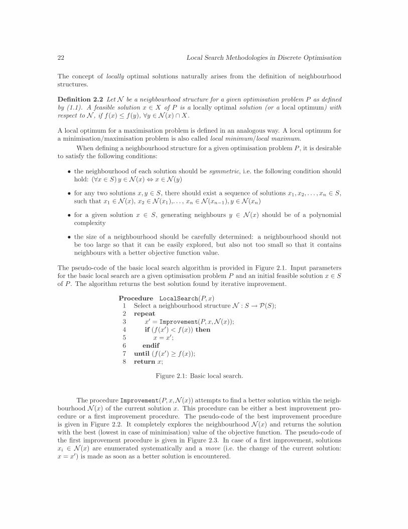
22 Local Search Methodologies in Discrete Optimisation
The concept of locally optimal solutions naturally arises from the definition of neighbourhoodstructures.
Definition 2.2 Let N be a neighbourhood structure for a given optimisation problem P as definedby (1.1). A feasible solution x ∈ X of P is a locally optimal solution (or a local optimum) withrespect to N , if f(x) ≤ f(y), ∀y ∈ N (x) ∩X.
A local optimum for a maximisation problem is defined in an analogous way. A local optimum fora minimisation/maximisation problem is also called local minimum/local maximum.
When defining a neighbourhood structure for a given optimisation problem P , it is desirableto satisfy the following conditions:
• the neighbourhood of each solution should be symmetric, i.e. the following condition shouldhold: (∀x ∈ S) y ∈ N (x)⇔ x ∈ N (y)
• for any two solutions x, y ∈ S, there should exist a sequence of solutions x1, x2, . . . , xn ∈ S,such that x1 ∈ N (x), x2 ∈ N (x1),. . . , xn ∈ N (xn−1), y ∈ N (xn)
• for a given solution x ∈ S, generating neighbours y ∈ N (x) should be of a polynomialcomplexity
• the size of a neighbourhood should be carefully determined: a neighbourhood should notbe too large so that it can be easily explored, but also not too small so that it containsneighbours with a better objective function value.
The pseudo-code of the basic local search algorithm is provided in Figure 2.1. Input parametersfor the basic local search are a given optimisation problem P and an initial feasible solution x ∈ Sof P . The algorithm returns the best solution found by iterative improvement.
Procedure LocalSearch(P, x)1 Select a neighbourhood structure N : S → P(S);2 repeat3 x′ = Improvement(P, x,N (x));4 if (f(x′) < f(x)) then5 x = x′;6 endif7 until (f(x′) ≥ f(x));8 return x;
Figure 2.1: Basic local search.
The procedure Improvement(P, x,N (x)) attempts to find a better solution within the neigh-bourhood N (x) of the current solution x. This procedure can be either a best improvement pro-cedure or a first improvement procedure. The pseudo-code of the best improvement procedureis given in Figure 2.2. It completely explores the neighbourhood N (x) and returns the solutionwith the best (lowest in case of minimisation) value of the objective function. The pseudo-code ofthe first improvement procedure is given in Figure 2.3. In case of a first improvement, solutionsxi ∈ N (x) are enumerated systematically and a move (i.e. the change of the current solution:x = x′) is made as soon as a better solution is encountered.
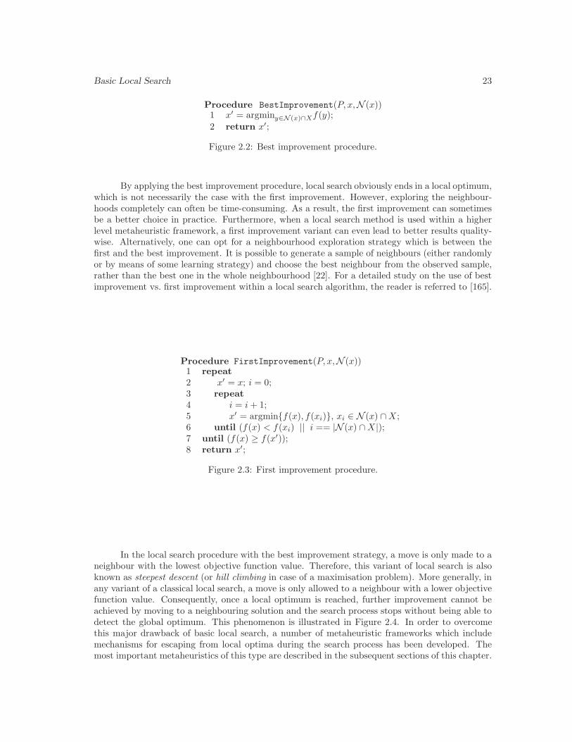
Basic Local Search 23
Procedure BestImprovement(P, x,N (x))1 x′ = argminy∈N (x)∩Xf(y);
2 return x′;
Figure 2.2: Best improvement procedure.
By applying the best improvement procedure, local search obviously ends in a local optimum,which is not necessarily the case with the first improvement. However, exploring the neighbour-hoods completely can often be time-consuming. As a result, the first improvement can sometimesbe a better choice in practice. Furthermore, when a local search method is used within a higherlevel metaheuristic framework, a first improvement variant can even lead to better results quality-wise. Alternatively, one can opt for a neighbourhood exploration strategy which is between thefirst and the best improvement. It is possible to generate a sample of neighbours (either randomlyor by means of some learning strategy) and choose the best neighbour from the observed sample,rather than the best one in the whole neighbourhood [22]. For a detailed study on the use of bestimprovement vs. first improvement within a local search algorithm, the reader is referred to [165].
Procedure FirstImprovement(P, x,N (x))1 repeat2 x′ = x; i = 0;3 repeat4 i = i + 1;5 x′ = argmin{f(x), f(xi)}, xi ∈ N (x) ∩X ;6 until (f(x) < f(xi) || i == |N (x) ∩X |);7 until (f(x) ≥ f(x′));8 return x′;
Figure 2.3: First improvement procedure.
In the local search procedure with the best improvement strategy, a move is only made to aneighbour with the lowest objective function value. Therefore, this variant of local search is alsoknown as steepest descent (or hill climbing in case of a maximisation problem). More generally, inany variant of a classical local search, a move is only allowed to a neighbour with a lower objectivefunction value. Consequently, once a local optimum is reached, further improvement cannot beachieved by moving to a neighbouring solution and the search process stops without being able todetect the global optimum. This phenomenon is illustrated in Figure 2.4. In order to overcomethis major drawback of basic local search, a number of metaheuristic frameworks which includemechanisms for escaping from local optima during the search process has been developed. Themost important metaheuristics of this type are described in the subsequent sections of this chapter.

24 Local Search Methodologies in Discrete Optimisation
x
local minimum
global minimum
x0
x2 x∗ x
optx
1
f(x)
Figure 2.4: Local search: stalling in a local optimum.
2.2 A Brief Overview of Local Search Based Metaheuristics
In this section some of the most important local search based metaheuristics are presented: simu-lated annealing (in Subsection 2.2.1), tabu search (in Subsection 2.2.2), greedy randomised adaptivesearch (in Subsection 2.2.3), guided local search (in Subsection 2.2.4) and iterated local search (inSubsection 2.2.5). As the research reported in this thesis is mainly based on variable neighbourhoodsearch, this metaheuristic is thoroughly discussed in the next section, where some new variableneighbourhood search schemes are also proposed.
2.2.1 Simulated Annealing
Simulated annealing (SA) is a metaheuristic which combines the principles of the basic local searchand the probabilistic Monte Carlo approach [143]. It is one of the oldest metaheuristic methods,originally proposed in [196] and [50]. In each iteration of SA, a neighbour of the current solution isgenerated at random and a move is made to this neighbouring solution depending on its objectivefunction value and the Metropolis criterion. If the selected neighbour has a better objective functionvalue than the current solution, it is automatically accepted and becomes the new current solution.Otherwise, the new solution is accepted according to the Metropolis criterion, i.e. with a certainprobability, which is systematically updated during the search process. The acceptance of worsesolutions provides the mechanism for avoiding the stalling in the local optima.
The motivation for the SA approach in combinatorial optimisation comes from the Metropo-lis algorithm in static thermodynamics [228]. The original Metropolis algorithm was used to sim-ulate the process of a solid material annealing: increasing the temperature of the material untilit is melted and then progressively reducing the temperature to recover a solid state of a lowerenergy. The appropriate cooling strategy is crucial for the success of the annealing process. If

Local Search Based Metaheuristics 25
the cooling is done too fast, it can cause irregularities in the material structure, which normallyresults in a high energy state. On the other hand, when cooling is done systematically, through anumber of levels so that the temperature is held long enough at each level to reach equilibrium,the more regular structures with low-energy states are obtained. In the context of combinatorialoptimisation, a solution of the problem corresponds to a state of the material, objective functionvalue corresponds to its energy, and a move to a neighbouring solution corresponds to the changeof the energy state. The general SA pseudo-code is provided in Figure 2.5.
Procedure SA(P )1 Choose initial solution x;2 Select a neighbourhood structure N : S → P(S);3 Set n = 0; Set proceed = true;4 while (proceed) do5 Choose x′ ∈ N (x) at random;6 if (f(x′) < f(x)) then7 x = x′;8 else9 Choose p ∈ [0, 1] at random;
10 if (p < exp((f(x)− f(x′))/tn)) then11 x = x′;12 endif13 endif14 n = n + 1;15 Update proceed;16 endwhile17 return x;
Figure 2.5: Simulated annealing.
The initial solution (line 1 in pseudo-code from Figure 2.5) is normally generated at randomor by means of some constructive heuristic (possibly problem-specific). Stopping criteria for thealgorithm are represented by the variable proceed (initialised in line 3 of SA pseudo-code). Mostoften, the stopping criteria include the maximum running time allowed, the maximum numberof iterations, or the maximum number of iterations without improvements. Variable p representsthe probability of acceptance and is determined in analogy to the physical annealing of solids,where a state change occurs with probability e−∆E/kt, ∆E being the change in energy, t thecurrent temperature, and k the Boltzmann constant. In the SA algorithm, the values of a so-called“temperature” parameter are defined by a sequence of positive numbers (tn), such that t0 ≥ t1 ≥ . . .and limn←∞ tn = 0. The sequence (tn) is called a cooling schedule. The temperature parameteris used to control the diversification during the search process. Large temperature values in thebeginning result in almost certain acceptance, therefore sampling the search space and avoidingthe local optima traps. Conversely, small temperature values near the end of the search resultin a very intensified exploration, rejecting almost all non-improving solutions. The most commoncooling schedule is a geometric sequence, where tn = αtn−1, for 0 < α < 1. This cooling schedulecorresponds to an exponential decrease of the temperature values. A more robust algorithm canbe obtained if the temperature is changed only after each L iterations, where L ∈ N is a predefinedparameter (usually determined according to the empirical experience) as in Figure 2.6. In thatcase, tn = αkt0, for kL ≤ n < (k + 1)L, k ∈ N ∪ {0}.
Over the years, more advanced SA schemes have been developed (see, for instance, [1, 3,
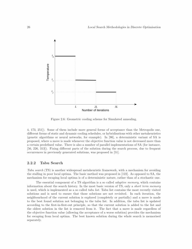
26 Local Search Methodologies in Discrete Optimisation
Number of iterations
Tem
pera
ture
t0
t1
t2
L 2L 3L
Figure 2.6: Geometric cooling scheme for Simulated annealing.
4, 173, 251]). Some of them include more general forms of acceptance than the Metropolis one,different forms of static and dynamic cooling schedules, or hybridisations with other metaheuristics(genetic algorithms or neural networks, for example). In [90], a deterministic variant of SA isproposed, where a move is made whenever the objective function value is not decreased more thana certain predefined value. There is also a number of parallel implementations of SA (for instance,[56, 226, 313]). Fixing different parts of the solution during the search process, due to frequentoccurrences in previously generated solutions, was proposed in [51].
2.2.2 Tabu Search
Tabu search (TS) is another widespread metaheuristic framework, with a mechanism for avoidingthe stalling in poor local optima. The basic method was proposed in [122]. As opposed to SA, themechanism for escaping local optima is of a deterministic nature, rather than of a stochastic one.
The essential component of a TS algorithm is a so called adaptive memory, which containsinformation about the search history. In the most basic version of TS, only a short term memoryis used, which is implemented as a so called tabu list. Tabu list contains the most recently visitedsolutions and is used to ensure that those solutions are not revisited. In each iteration, theneighbourhood of the current solution is explored (completely or partially) and a move is madeto the best found solution not belonging to the tabu list. In addition, the tabu list is updatedaccording to the first-in-first-out principle, so that the current solution is added to the list andthe oldest solution in the list is removed from it. The fact that a move is made regardless ofthe objective function value (allowing the acceptance of a worse solution) provides the mechanismfor escaping from local optima. The best known solution during the whole search is memorisedseparately.

Local Search Based Metaheuristics 27
Clearly, the crucial parameter which controls the extent of the diversification and intensifi-cation is the length of the tabu list. If the tabu list is short, the search concentrates on small areasof the solution space. Conversely, a long tabu list forbids a larger number of solutions and thusensures the exploration of larger regions. In a more advanced framework, the length of the tabulist can be varied during the search, resulting in a more robust algorithm.
An implementation of the tabu list which keeps complete solutions is often inefficient. Itis obviously space consuming, but also requires a long time for browsing the list. This drawbackis usually overcome by storing only a set of preselected solution attributes instead of a completesolution. However, storing only a set of attributes may result in a loss of information, since theprohibition of a single attribute usually forces more than one solution to be added to the tabu list.This way, unvisited solutions of a good quality may be excluded from the further search. The mostcommon solution to this problem is to introduce the set of so called aspiration criteria, so thata move to a solution in the tabu list is permitted whenever the solution satisfies some aspirationcriterion. The simplest example of an aspiration criterion is the one which permits solutions betterthan the currently best known solution. This criterion is defined by f(x) < f(x∗) for a givensolution x, where x∗ is the currently best solution. The basic form of the tabu search algorithm isprovided in Figure 2.7, where P is an input optimisation problem as defined by (1.1).
Procedure TS(P )1 Choose initial solution x;2 Memorise best solution so far: x∗ = x;3 Select a neighbourhood structure N : S → P(S);4 Initialise tabu list TL;5 Initialise the set of aspiration criteria AC;6 Set proceed = true;7 while (proceed) do8 Choose the best
x′ ∈ N (x) ∩ {x ∈ X | x /∈ TL or x satisfies at least one criterion from AC};9 x = x′;
10 if (f(x) < f(x∗)) then x∗ = x; endif;11 Update TL; Update AC;12 Update proceed;13 endwhile14 return x∗;
Figure 2.7: Tabu search.
A variety of extensions and enhancements of the basic TS scheme has been proposed since itwas first originated in 1986. One of the most significant and widespread improvements is the use ofa long term memory [131]. Normally, the long term memory is based on (some of) the following fourprinciples: recency, frequency, quality and influence [37]. Recency-based memory keeps track ofthe most recent relevant iteration for each solution. Frequency-based memory stores the numberof times each solution was visited. The quality-based memory records the information aboutthe good solutions/solution attributes visited during the search process. Lastly, influence-basedmemory keeps track of critical choices made during the search and is normally exploited to indicatethe choices of interest. By using a long term memory, a much better control over the processesof diversification and intensification can be achieved than by means of a short term memory.Diversification is enforced by generating solutions with combinations of attributes significantlydifferent from those previously encountered. On the other hand, intensification is propagated

28 Local Search Methodologies in Discrete Optimisation
by incorporating the attributes of good-quality solutions (so called elite solutions) stored in thememory. Another interesting approach is the integration of TS and path relinking [131, 132],where new solutions are created by exploring the paths between elite solutions. In probabilisticTS [131], candidate solutions are selected at random from an appropriate neighbourhood, ratherthan deterministically as in the classical TS. This speeds up the neighbourhood exploration and atthe same time increases the level of diversification. An especially interesting class of advanced TSalgorithms are so called reactive techniques, which provide a mechanism for a dynamic adjustmentof parameters during the search process [23, 227, 323]. In this context, the parameter of thegreatest interest is usually the length of the tabu list. Finally, numerous hybridisations of TS withother metaheuristics have been developed. There are known hybrids with genetic algorithms [126],memetic algorithms [217], ant colony optimisation [15], etc. (the stated references are only fewpossible examples).
2.2.3 Greedy Randomised Adaptive Search
Greedy randomised adaptive search (GRASP) is a multi-start (i.e. iterative) algorithm, where anew solution is generated in a two-stage process at each restart (iteration), and the best overallsolution is returned as a result. The two-stage process involves construction as the first phase andlocal search improvement as the second phase. The basic algorithm was proposed in [102], followedby enhanced versions in [260, 280].
The pseudo-code of the basic GRASP algorithm is provided in Figure 2.8. In the constructionstage (lines 6–12), a new solution is constructed progressively, by adding one new component ineach iteration. First, all candidate elements for the next component of the current solution xare evaluated (line 7 of the pseudo-code from Figure 2.8). The evaluation is performed accordingto a candidate’s contribution to the objective function value, if inserted into the current partialsolution x. Then, a so called restricted candidate list (RCL) is formed, so that it contains the best αcomponent candidates (lines 8–9 of the pseudo-code from Figure 2.8). The next solution componentxk is chosen at random from the so obtained restricted candidate list, and added to the currentpartial solution. This process is iterated as long as the current solution x is not complete. Theconstruction stage is essentially a greedy randomised procedure: it considers the best α candidates(a greedy approach) and employs randomization to select one of them. Obviously, the RCL lengthα is the crucial parameter for the algorithm, since it controls the level of randomization andtherefore the level of diversification during the search process. If α = 1, the best element is added,so the construction is equivalent to a deterministic greedy heuristic. Conversely, when α = n,the construction is entirely random. The second stage of the algorithm consists of a local searchprocedure, with the constructed solution x as an initial solution (line 13 of the pseudo-code fromFigure 2.8). This local search procedure may be the basic LS algorithm from Section 2.1, or a moreadvanced technique, such as simulated annealing, tabu search, variable neighbourhood search, etc.The two stages of GRASP are iterated as long as the stopping criteria, represented by the variableproceed, are not fulfilled.
The main drawback of the basic GRASP algorithm is that the solution processes in differentrestarts are completely independent, and the information from previous restarts is not available at acertain point of search. A number of GRASP enhancements have been developed which addressesthis issue. The use of a long term memory within GRASP was proposed in [107]. Anotherpossibility to incorporate memory within the GRASP search process is a reactive approach, inwhich the parameter α is selected from a set of values depending on the solution values from theprevious restarts [13, 263, 264]. A variety of other enhancements of GRASP has also been designed.The employment of path relinking as an intensification strategy within GRASP was proposed in[200]. Some examples of parallel implementations, where the restarts are distributed over multiple

Local Search Based Metaheuristics 29
Procedure GRASP(P )1 Select a neighbourhood structure N : S → P(S);2 Set n to the number of solution components;3 Set proceed = true;4 while (proceed) do5 x = ∅;6 for (k = 1; k <= n; k + +) do7 Evaluate the candidate components;8 Determine the length α of the restricted candidate list;9 Build the restricted candidate list RCLα for x;
10 Select xk ∈ RCLα at random;11 x = x ∪ {xk};12 endfor13 x′ = LocalSearch(P, x);14 if ((x∗ not yet assigned) || (f(x′) < f(x∗))) then15 x∗ = x′;16 endif;17 Update proceed;18 endwhile19 return x∗;
Figure 2.8: Greedy randomised adaptive search.
processors, can be found in [244, 256, 257]. Due to its simplicity, the GRASP algorithm is usuallyvery fast and produces reasonable-quality solutions in a short time. Therefore, it is especiallyconvenient for integration with other metaheuristics. A hybridisation with variable neighbourhoodsearch [224] can be distinguished as one interesting example.
2.2.4 Guided Local Search
All metaheuristics discussed so far provide a mechanism for escaping from local optima through anintelligent construction of search trajectories for a fixed problem structure. In contrast, guided localsearch (GLS) metaheuristic guides the search away from local optima by changing the objectivefunction of the problem, i.e. modifying the search landscape itself [318, 319]. The GLS strategyexploits so called solution features to discriminate between solutions and thus appropriately aug-ment the objective function value in order to reposition the local optima. The general scheme isillustrated in Figure 2.9.
The pseudo-code of the basic GLS framework is provided in Figure 2.10. After the initialsolution and the neighbourhood structure are selected (lines 1–2 in Figure 2.10), the vector ofpenalties p = (p1, p2, . . . , pk) is initialised, where k is the number of solution features considered(line 3 in Figure 2.10). Penalties represent the feature weights: the higher the penalty value pi, thehigher the importance of feature i. Stopping criteria are defined by the variable proceed (line 4 inFigure 2.10). In each iteration of the algorithm, the objective function is increased with respect tothe current penalty values (line 6 in Figure 2.10), according to the formula:
(2.1) f ′(x) = f(x) + λ
k∑
i=1
piIi(x).

30 Local Search Methodologies in Discrete Optimisation
x
f(x)
xminnew
xminold
Figure 2.9: GLS: escaping from local minimum by increasing the objective function value.
Function Ii(x) indicates whether the ith feature is present in the current solution x:
(2.2) Ii(x) =
{1 if the ith feature is present in x,0 otherwise.
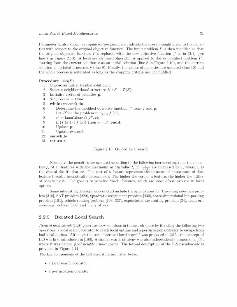
Local Search Based Metaheuristics 31
Parameter λ, also known as regularisation parameter, adjusts the overall weight given to the penal-ties with respect to the original objective function. The input problem P is then modified so thatthe original objective function f is replaced with the new objective function f ′ as in (2.1) (seeline 7 in Figure 2.10). A local search based algorithm is applied to the so modified problem P ′,starting from the current solution x as an initial solution (line 8 in Figure 2.10), and the currentsolution is updated if necessary (line 9). Finally, the values of penalties are updated (line 10) andthe whole process is reiterated as long as the stopping criteria are not fulfilled.
Procedure GLS(P )1 Choose an initial feasible solution x;2 Select a neighbourhood structure N : S → P(S);3 Initialise vector of penalties p;4 Set proceed = true;5 while (proceed) do6 Determine the modified objective function f ′ from f and p;7 Let P ′ be the problem minx∈X f ′(x);8 x′ = LocalSearch(P ′, x);9 if (f ′(x′) < f ′(x)) then x = x′; endif;
10 Update p;11 Update proceed;12 endwhile13 return x;
Figure 2.10: Guided local search.
Normally, the penalties are updated according to the following incrementing rule: the penal-ties pi of all features with the maximum utility value Ii(x) · ci
1+piare increased by 1, where ci is
the cost of the ith feature. The cost of a feature represents the measure of importance of thatfeature (usually heuristically determined). The higher the cost of a feature, the higher the utilityof penalising it. The goal is to penalise “bad” features, which are most often involved in localoptima.
Some interesting developments of GLS include the applications for Travelling salesman prob-lem [318], SAT problem [229], Quadratic assignment problem [230], three-dimensional bin-packingproblem [101], vehicle routing problem [193, 337], capacitated arc-routing problem [34], team ori-enteering problem [309] and many others.
2.2.5 Iterated Local Search
Iterated local search (ILS) generates new solutions in the search space by iterating the following twooperators: a local search operator to reach local optima and a perturbation operator to escape frombad local optima. Although the term “iterated local search” was proposed in [215], the concept ofILS was first introduced in [188]. A similar search strategy was also independently proposed in [45],where it was named fixed neighbourhood search. The formal description of the ILS pseudo-code isprovided in Figure 2.11.
The key components of the ILS algorithm are listed below:
• a local search operator
• a perturbation operator
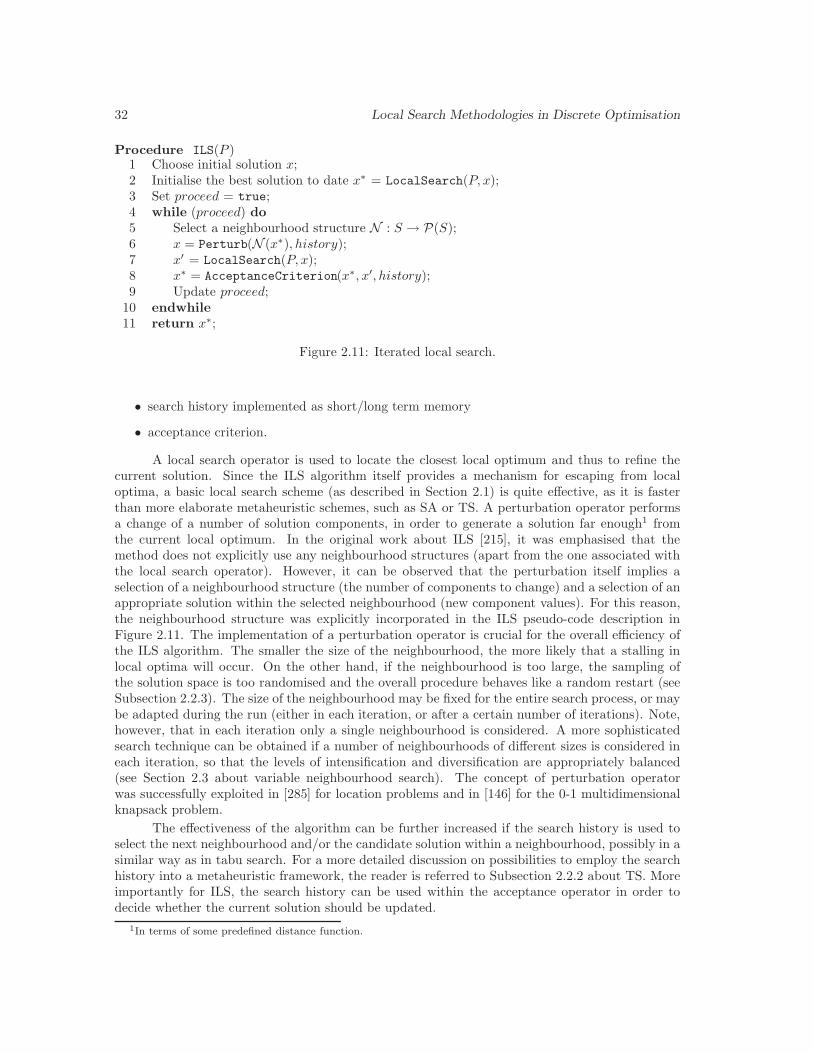
32 Local Search Methodologies in Discrete Optimisation
Procedure ILS(P )1 Choose initial solution x;2 Initialise the best solution to date x∗ = LocalSearch(P, x);3 Set proceed = true;4 while (proceed) do5 Select a neighbourhood structure N : S → P(S);6 x = Perturb(N (x∗), history);7 x′ = LocalSearch(P, x);8 x∗ = AcceptanceCriterion(x∗, x′, history);9 Update proceed;
10 endwhile11 return x∗;
Figure 2.11: Iterated local search.
• search history implemented as short/long term memory
• acceptance criterion.
A local search operator is used to locate the closest local optimum and thus to refine thecurrent solution. Since the ILS algorithm itself provides a mechanism for escaping from localoptima, a basic local search scheme (as described in Section 2.1) is quite effective, as it is fasterthan more elaborate metaheuristic schemes, such as SA or TS. A perturbation operator performsa change of a number of solution components, in order to generate a solution far enough1 fromthe current local optimum. In the original work about ILS [215], it was emphasised that themethod does not explicitly use any neighbourhood structures (apart from the one associated withthe local search operator). However, it can be observed that the perturbation itself implies aselection of a neighbourhood structure (the number of components to change) and a selection of anappropriate solution within the selected neighbourhood (new component values). For this reason,the neighbourhood structure was explicitly incorporated in the ILS pseudo-code description inFigure 2.11. The implementation of a perturbation operator is crucial for the overall efficiency ofthe ILS algorithm. The smaller the size of the neighbourhood, the more likely that a stalling inlocal optima will occur. On the other hand, if the neighbourhood is too large, the sampling ofthe solution space is too randomised and the overall procedure behaves like a random restart (seeSubsection 2.2.3). The size of the neighbourhood may be fixed for the entire search process, or maybe adapted during the run (either in each iteration, or after a certain number of iterations). Note,however, that in each iteration only a single neighbourhood is considered. A more sophisticatedsearch technique can be obtained if a number of neighbourhoods of different sizes is considered ineach iteration, so that the levels of intensification and diversification are appropriately balanced(see Section 2.3 about variable neighbourhood search). The concept of perturbation operatorwas successfully exploited in [285] for location problems and in [146] for the 0-1 multidimensionalknapsack problem.
The effectiveness of the algorithm can be further increased if the search history is used toselect the next neighbourhood and/or the candidate solution within a neighbourhood, possibly in asimilar way as in tabu search. For a more detailed discussion on possibilities to employ the searchhistory into a metaheuristic framework, the reader is referred to Subsection 2.2.2 about TS. Moreimportantly for ILS, the search history can be used within the acceptance operator in order todecide whether the current solution should be updated.
1In terms of some predefined distance function.
Variable Neighbourhood Search 33
The acceptance criterion has a great impact on the behaviour of the ILS search process.In particular, the balance between the diversification and intensification largely depends on theacceptance rule. For instance, the criterion which accepts the new local optimum only if it isbetter than the currently best solution, obviously favours the intensification. Conversely, alwaysaccepting the new local optimum, regardless of the objective function value, leads to an extremelydiversified search. One possible intermediate choice between these two extremes is the use of an SA-type acceptance criterion: accepting the new local optimum if it is better than the currently bestone and otherwise applying the Metropolis criterion (see Subsection 2.2.1). Another interestingpossibility is to use a non-monotonic cooling schedule within the SA-type criterion explained above,together with the search history: instead of constantly decreasing the temperature, it is increasedwhen more diversification is required.
Some of the interesting developments and applications of the ILS algorithm can be found in[181, 300, 303, 304].
2.3 Variable Neighbourhood Search
All local search based metaheuristics discussed so far deal only with a single neighbourhood struc-ture in each iteration, which may or may not be updated from one iteration to another. However,the selection of the neighbourhood structure is essential for the effectiveness of the search process,as was already mentioned in Subsection 2.2.5. Therefore, the solution process can be significantlyimproved if more than one neighbourhood of the currently observed solution is explored and thusa few new candidate solutions are generated in each iteration. This is the basic idea of the variableneighbourhood search metaheuristic [159, 161, 162, 164, 166, 167, 237].
Variable neighbourhood search (VNS) was first proposed in 1997 (see [237]) and has led tomany developments and applications since. The idea for a systematic change of neighbourhoods,performed by VNS, is based on the following facts (see [167]):
Fact 1 A local optimum with respect to one neighbourhood structure is not necessarily a localoptimum with respect to another neighbourhood structure.
Fact 2 A global optimum is a local optimum with respect to any neighbourhood structure.
Fact 3 Local optima with respect to one or several neighbourhood structures are relatively closeto each other.
The last fact relies on the empirical experience: extensive experimental analysis for a huge varietyof different problems suggests that local optima frequently contain some information about theglobal optimum. For example, it appears that some variables usually have the same values in bothlocal and global optima.
VNS has a number of specific variants, depending on the selection of neighbourhood struc-tures, neighbourhood change scheme, selection of candidate solutions within a neighbourhood,updating the incumbent solution, etc. In the remainder of this section, the most significant vari-ants of VNS are described in detail. Subsection 2.3.1 is devoted to the well-established VNSschemes. Subsection 2.3.2 aims to provide an insight into more elaborate solution methodologies,with some notable contributions to the metaheuristics development in general. Some new VNSschemes are also proposed.
2.3.1 Basic Schemes
Variable neighbourhood search deals with a set of more than one neighbourhood structures ateach iteration, rather than with a single neighbourhood structure (see Figure 2.12). Furthermore,

34 Local Search Methodologies in Discrete Optimisation
in a nested VNS framework, where some VNS scheme is used as a local search operator withinanother VNS scheme, different sets of neighbourhood structures may be used for the two schemes.In further text, {Nk : S → P(S) | 1 ≤ kmin ≤ k ≤ kmax}, kmin, kmax ∈ N, will denote the set ofpreselected neighbourhood structures for the main VNS scheme of interest.
Figure 2.12: The change of the used neighbourhood in some typical VNS solution trajectory.
Usually, neighbourhood structures Nk, 1 ≤ kmin ≤ k ≤ kmax are induced by one or moremetric (or quasi-metric2) functions of the form ρ : S2 → R+, defined in the solution space S:
(2.3) Nk(x) = {y ∈ X | ρ(x, y) ≤ k}.
Definition (2.3) implies that the neighbourhoods are nested, i.e. Nk(x) ⊂ Nk+1(x), for any x ∈ Sand appropriate value of k. There are, however, other possibilities to define distance-inducedneighbourhood structures. If the solution space S is discrete, condition ρ(x, y) ≤ k in definition(2.3) can be replaced with ρ(x, y) = k. If the solution space S is continuous, condition ρ(x, y) ≤ kis commonly replaced with k− 1 ≤ ρ(x, y) < k. The choice of neighbourhood structures dependson the problem of interest and the final requirement (whether the most important issue for theend user is the execution time, solution quality, etc.). In a more advanced environment, theneighbourhood structures to be used can even be changed from one iteration to another.
In order to solve problem (1.1) by exploring several neighbourhoods in each iteration, facts 1to 3 can be combined in three different ways to balance between diversification and intensification:(i) deterministic; (ii) stochastic; (iii) both deterministic and stochastic. The resulting VNS variantsare described in the subsequent subsections.
Variable Neighbourhood Descent
Variable neighbourhood descent (VND) is obtained if all neighbourhoods generated during thesearch are explored completely [159]. The VND pseudo-code is provided in Figure 2.13, withprocedure BestImprovement(P, x,Nk(x)) as in Figure 2.2 in Section 2.1. The input parametersfor the VND algorithm are an optimisation problem P as defined in (1.1), the initial solution x andthe maximum number kvnd of neighbourhoods (of a single solution) to explore. The best solutionfound is returned as the result.
2Where the symmetry requirement is dropped.
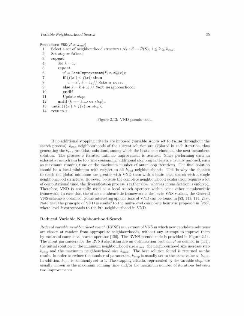
Variable Neighbourhood Search 35
Procedure VND(P, x, kvnd)1 Select a set of neighbourhood structures Nk : S → P(S), 1 ≤ k ≤ kvnd;2 Set stop = false;3 repeat4 Set k = 1;5 repeat6 x′ = BestImprovement(P, x,Nk(x));7 if (f(x′) < f(x)) then8 x = x′, k = 1; // Make a move.
9 else k = k + 1; // Next neighbourhood.
10 endif11 Update stop;12 until (k == kvnd or stop);13 until (f(x′) ≥ f(x) or stop);14 return x.
Figure 2.13: VND pseudo-code.
If no additional stopping criteria are imposed (variable stop is set to false throughout thesearch process), kvnd neighbourhoods of the current solution are explored in each iteration, thusgenerating the kvnd candidate solutions, among which the best one is chosen as the next incumbentsolution. The process is iterated until no improvement is reached. Since performing such anexhaustive search can be too time consuming, additional stopping criteria are usually imposed, suchas maximum running time or the maximum number of outer loop iterations. The final solutionshould be a local minimum with respect to all kvnd neighbourhoods. This is why the chancesto reach the global minimum are greater with VND than with a basic local search with a singleneighbourhood structure. However, because the complete neighbourhood exploration requires a lotof computational time, the diversification process is rather slow, whereas intensification is enforced.Therefore, VND is normally used as a local search operator within some other metaheuristicframework. In case that the other metaheuristic framework is the basic VNS variant, the GeneralVNS scheme is obtained. Some interesting applications of VND can be found in [53, 113, 174, 248].Note that the principle of VND is similar to the multi-level composite heuristic proposed in [286],where level k corresponds to the kth neighbourhood in VND.
Reduced Variable Neighbourhood Search
Reduced variable neighbourhood search (RVNS) is a variant of VNS in which new candidate solutionsare chosen at random from appropriate neighbourhoods, without any attempt to improve themby means of some local search operator [159]. The RVNS pseudo-code is provided in Figure 2.14.The input parameters for the RVNS algorithm are an optimisation problem P as defined in (1.1),the initial solution x, the minimum neighbourhood size kmin, the neighbourhood size increase stepkstep and the maximum neighbourhood size kmax. The best solution found is returned as theresult. In order to reduce the number of parameters, kstep is usually set to the same value as kmin.In addition, kmin is commonly set to 1. The stopping criteria, represented by the variable stop, areusually chosen as the maximum running time and/or the maximum number of iterations betweentwo improvements.
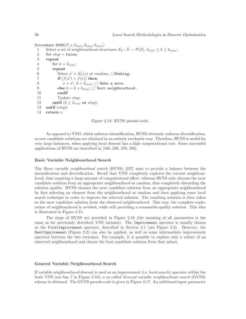
36 Local Search Methodologies in Discrete Optimisation
Procedure RVNS(P, x, kmin, kstep, kmax)1 Select a set of neighbourhood structures Nk : S → P(S), kmin ≤ k ≤ kmax;2 Set stop = false;3 repeat4 Set k = kmin;5 repeat6 Select x′ ∈ Nk(x) at random; //Shaking.7 if (f(x′) < f(x)) then8 x = x′, k = kmin; // Make a move.
9 else k = k + kstep; // Next neighbourhood.
10 endif11 Update stop;12 until (k ≥ kmax or stop);13 until (stop);14 return x.
Figure 2.14: RVNS pseudo-code.
As opposed to VND, which enforces intensification, RVNS obviously enforces diversification,as new candidate solutions are obtained in an entirely stochastic way. Therefore, RVNS is useful forvery large instances, when applying local descent has a high computational cost. Some successfulapplications of RVNS are described in [160, 238, 278, 293].
Basic Variable Neighbourhood Search
The Basic variable neighbourhood search (BVNS) [237] aims to provide a balance between theintensification and diversification. Recall that VND completely explores the current neighbour-hood, thus requiring a large amount of computational effort, whereas RVNS only chooses the nextcandidate solution from an appropriate neighbourhood at random, thus completely discarding thesolution quality. BVNS chooses the next candidate solution from an appropriate neighbourhoodby first selecting an element from the neighbourhood at random and then applying some localsearch technique in order to improve the selected solution. The resulting solution is then takenas the next candidate solution from the observed neighbourhood. This way, the complete explo-ration of neighbourhood is avoided, while still providing a reasonable-quality solution. This ideais illustrated in Figure 2.15.
The steps of BVNS are provided in Figure 2.16 (the meaning of all parameters is thesame as for previously described VNS variants). The Improvement operator is usually chosenas the FirstImprovement operator, described in Section 2.1 (see Figure 2.3). However, theBestImprovement (Figure 2.2) can also be applied, as well as some intermediate improvementoperator between the two extremes. For example, it is possible to explore only a subset of anobserved neighbourhood and choose the best candidate solution from that subset.
General Variable Neighbourhood Search
If variable neighbourhood descent is used as an improvement (i.e. local search) operator within thebasic VNS (see line 7 in Figure 2.16), a so called General variable neighbourhood search (GVNS)scheme is obtained. The GVNS pseudo-code is given in Figure 2.17. An additional input parameter
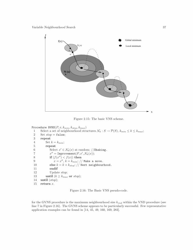
Variable Neighbourhood Search 37
N1(x)
f
x
x’
f(x)
x
N (x)k
Global minimum
Local minimum
Figure 2.15: The basic VNS scheme.
Procedure BVNS(P, x, kmin, kstep, kmax)1 Select a set of neighbourhood structures Nk : S → P(S), kmin ≤ k ≤ kmax;2 Set stop = false;3 repeat4 Set k = kmin;5 repeat6 Select x′ ∈ Nk(x) at random; //Shaking.7 x′′ = Improvement(P, x′,Nk(x));8 if (f(x′′) < f(x)) then9 x = x′′, k = kmin; // Make a move.
10 else k = k + kstep; // Next neighbourhood.
11 endif12 Update stop;13 until (k ≥ kmax or stop);14 until (stop);15 return x.
Figure 2.16: The Basic VNS pseudo-code.
for the GVNS procedure is the maximum neighbourhood size kvnd within the VND procedure (seeline 7 in Figure 2.16). The GVNS scheme appears to be particularly successful. Few representativeapplication examples can be found in [14, 45, 49, 160, 169, 283].
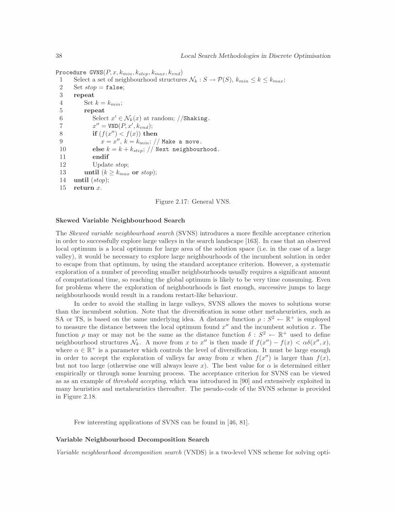
38 Local Search Methodologies in Discrete Optimisation
Procedure GVNS(P, x, kmin, kstep, kmax, kvnd)1 Select a set of neighbourhood structures Nk : S → P(S), kmin ≤ k ≤ kmax;2 Set stop = false;3 repeat4 Set k = kmin;5 repeat6 Select x′ ∈ Nk(x) at random; //Shaking.7 x′′ = VND(P, x′, kvnd);8 if (f(x′′) < f(x)) then9 x = x′′, k = kmin; // Make a move.
10 else k = k + kstep; // Next neighbourhood.
11 endif12 Update stop;13 until (k ≥ kmax or stop);14 until (stop);15 return x.
Figure 2.17: General VNS.
Skewed Variable Neighbourhood Search
The Skewed variable neighbourhood search (SVNS) introduces a more flexible acceptance criterionin order to successfully explore large valleys in the search landscape [163]. In case that an observedlocal optimum is a local optimum for large area of the solution space (i.e. in the case of a largevalley), it would be necessary to explore large neighbourhoods of the incumbent solution in orderto escape from that optimum, by using the standard acceptance criterion. However, a systematicexploration of a number of preceding smaller neighbourhoods usually requires a significant amountof computational time, so reaching the global optimum is likely to be very time consuming. Evenfor problems where the exploration of neighbourhoods is fast enough, successive jumps to largeneighbourhoods would result in a random restart-like behaviour.
In order to avoid the stalling in large valleys, SVNS allows the moves to solutions worsethan the incumbent solution. Note that the diversification in some other metaheuristics, such asSA or TS, is based on the same underlying idea. A distance function ρ : S2 ← R+ is employedto measure the distance between the local optimum found x′′ and the incumbent solution x. Thefunction ρ may or may not be the same as the distance function δ : S2 ← R+ used to defineneighbourhood structures Nk. A move from x to x′′ is then made if f(x′′) − f(x) < αδ(x′′, x),where α ∈ R+ is a parameter which controls the level of diversification. It must be large enoughin order to accept the exploration of valleys far away from x when f(x′′) is larger than f(x),but not too large (otherwise one will always leave x). The best value for α is determined eitherempirically or through some learning process. The acceptance criterion for SVNS can be viewedas as an example of threshold accepting, which was introduced in [90] and extensively exploited inmany heuristics and metaheuristics thereafter. The pseudo-code of the SVNS scheme is providedin Figure 2.18.
Few interesting applications of SVNS can be found in [46, 81].
Variable Neighbourhood Decomposition Search
Variable neighbourhood decomposition search (VNDS) is a two-level VNS scheme for solving opti-

Variable Neighbourhood Search 39
Procedure SVNS(P, x, kmin, kstep, kmax, kvnd)1 Select a set of neighbourhood structures Nk : S → P(S), kmin ≤ k ≤ kmax;2 Set stop = false;3 repeat4 Set k = kmin;5 repeat6 Select x′ ∈ Nk(x) at random; //Shaking.7 x′′ = VND(P, x′, kvnd);8 if (f(x′′)− f(x) < αδ(x′′, x)) then9 x = x′′, k = kmin; // Make a move.
10 else k = k + kstep; // Next neighbourhood.
11 endif12 Update stop;13 until (k ≥ kmax or stop);14 until (stop);15 return x.
Figure 2.18: Skewed VNS.
misation problems, based upon the decomposition of the problem [168]. The motivation for thisvariant of VNS comes from the difficulty to solve large instances of combinatorial optimisationproblems, where basic VNS fails to provide solutions of good quality in reasonable computationaltime. The basic idea of VNDS is to restrict the search process to only a subspace of the entire searchspace (usually defined by some subset of solution attributes), which can be efficiently explored.
LetA be the set of all solution attributes, J ⊆ A an arbitrary subset ofA and x(J) = (xj)j∈J
the sub-vector associated with the set of solution attributes J and solution x. If P is a givenoptimisation problem, as defined by (1.1), then the reduced problem P (x0, J), associated with thearbitrary feasible solution x0 ∈ X and the subset of solution attributes J ⊆ A, can be defined as:
(2.4) min{f(x) | x ∈ X, xj = x0
j , ∀j ∈ J}.
The steps of the VNDS method are presented in Fig. 2.19.
At each iteration, VNDS chooses randomly a subset of solution attributes Jk ⊆ A withcardinality k. Then a local search is applied to the subproblem P (x, Jk), Jk = A \ Jk, wherevariables containing attributes from Jk are fixed to values of the current incumbent solution x.The operator LocalSearch(P (x, Jk), x(Jk)) (line 6 in Figure 2.19) can be the basic local searchmethod as described in Section 2.1, but also any other local search based metaheuristic method.Other VNS schemes are most commonly used for this purpose. The local search starts from thecurrent solution x(Jk), to obtain the final solution x′ and it operates only on the sub-vector x(Jk)(i.e., on the free variables indexed by Jk). If an improvement occurs, a local search is performed onthe complete solution, starting from x′, in order to refine the obtained local optimum x′. Again,the local search applied at this stage is usually some other VNS scheme. For the purpose ofrefinement, it is necessary to intensify the search. Therefore, the VND variant is the best choicein the majority of cases. The whole process is iterated until the fulfilment of stopping criteria. Asin the previously described VNS variants, stopping criteria normally represent the running timelimitations, the total number of iterations or the number of iterations between two improvements.
The VNDS approach is becoming increasingly popular, with a number of successful appli-cations arising [68, 158, 207, 209, 308].
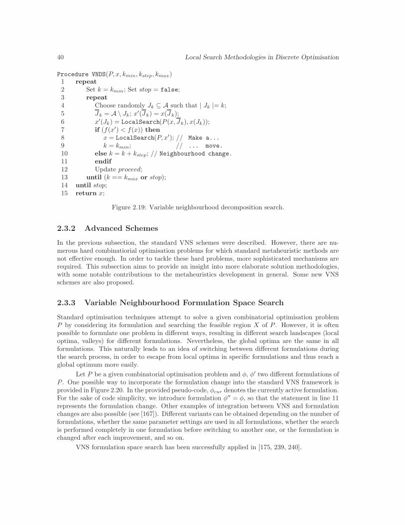
40 Local Search Methodologies in Discrete Optimisation
Procedure VNDS(P, x, kmin, kstep, kmax)1 repeat2 Set k = kmin; Set stop = false;3 repeat4 Choose randomly Jk ⊆ A such that | Jk |= k;5 Jk = A \ Jk; x′(Jk) = x(Jk);6 x′(Jk) = LocalSearch(P (x, Jk), x(Jk));7 if (f(x′) < f(x)) then8 x = LocalSearch(P, x′); // Make a...
9 k = kmin; // ... move.
10 else k = k + kstep; // Neighbourhood change.
11 endif12 Update proceed;13 until (k == kmax or stop);14 until stop;15 return x;
Figure 2.19: Variable neighbourhood decomposition search.
2.3.2 Advanced Schemes
In the previous subsection, the standard VNS schemes were described. However, there are nu-merous hard combinatiorial optimisation problems for which standard metaheuristic methods arenot effective enough. In order to tackle these hard problems, more sophisticated mechanisms arerequired. This subsection aims to provide an insight into more elaborate solution methodologies,with some notable contributions to the metaheuristics development in general. Some new VNSschemes are also proposed.
2.3.3 Variable Neighbourhood Formulation Space Search
Standard optimisation techniques attempt to solve a given combinatorial optimisation problemP by considering its formulation and searching the feasible region X of P . However, it is oftenpossible to formulate one problem in different ways, resulting in different search landscapes (localoptima, valleys) for different formulations. Nevertheless, the global optima are the same in allformulations. This naturally leads to an idea of switching between different formulations duringthe search process, in order to escape from local optima in specific formulations and thus reach aglobal optimum more easily.
Let P be a given combinatorial optimisation problem and φ, φ′ two different formulations ofP . One possible way to incorporate the formulation change into the standard VNS framework isprovided in Figure 2.20. In the provided pseudo-code, φcur denotes the currently active formulation.For the sake of code simplicity, we introduce formulation φ′′ = φ, so that the statement in line 11represents the formulation change. Other examples of integration between VNS and formulationchanges are also possible (see [167]). Different variants can be obtained depending on the number offormulations, whether the same parameter settings are used in all formulations, whether the searchis performed completely in one formulation before switching to another one, or the formulation ischanged after each improvement, and so on.
VNS formulation space search has been successfully applied in [175, 239, 240].

Variable Neighbourhood Search 41
Procedure VNS-FSS(P, φ, φ′, x, kmin, kstep, kmax)1 Set stop = false, φcur = φ;2 Select neighbourhood structures Nk,φ : Sφ → P(Sφ), kmin ≤ k ≤ kmax;3 Select neighbourhood structures Nk,φ′ : Sφ′ → P(Sφ′), kmin ≤ k ≤ kmax;4 repeat5 Set k = kmin;6 repeat7 Select x′ ∈ Nk,φcur
(x) at random;8 x′′ = Improvement(P, x′,Nk,φcur
(x));9 if (f(x′′, φcur) < f(x, φcur)) then10 x = x′′, k = kmin; // Make a move.
11 if (φcur == φ) then // Change formulation.
12 (φcur = φ′)13 else (φcur = φ)14 endif15 else k = k + kstep; // Next neighbourhood.
16 Update stop;17 until (k ≥ kmax or stop);18 until (stop);19 return x.
Figure 2.20: VNS formulation space search.
2.3.4 Primal-dual VNS
As already discussed in Chapter 1, heuristic methods cannot guarantee the solution optimality andoften cannot provide the information about how close to optimality a particular heuristic solution is.In case of mathematical programming, the standard approach is to relax the integrality constraintson the primal variables, in order to determine the lower3 bound for the optimal solution. Yet, forvery large problem instances, even the relaxed problem could be impossible to solve to optimalityusing standard commercial solvers. Hence, one must look for alternatives for gaining the guaranteedbounds for the optimal solution of the original primal problem. One promising possibility is tosolve dual relaxed problems heuristically as well and thus iterate the solution processes for primaland dual problems. This approach has been successfully combined with VNS for solving the large-scale simple plant location problems [155]. The resulting primal-dual VNS (PD-VNS) iterates thefollowing three stages:
1) find an initial dual solution (generally infeasible), using the primal heuristic solution andcomplementary slackness conditions
2) improve the solution by applying VNS to the unconstrained nonlinear form of the dual
3) solve the dual exactly
For more details on PD-VNS, the reader is referred to [155, 167].
3In the context of minimisation.

42 Local Search Methodologies in Discrete Optimisation
2.3.5 Dynamic Selection of Parameters and/or Neighbourhood Struc-tures
Any local search based metaheuristic method is characterised by the following three components,apart from the initial solution supplied: 1) problem formulation, 2) definition of neighbourhoodstructures and 3) set of method-specific parameters. In standard optimisation techniques, thesecomponents are kept fixed during the search process. However, the behaviour of the search processchanges with time, as the solution approaches the optimum, and the initial settings of the abovementioned components are usually not so effective in the middle or near the end of the searchprocess. Moreover, it normally takes a great amount of preliminary tests to determine the bestsettings at the beginning. Therefore, an appropriate on-the-way update of these components duringthe search process can be highly beneficial. Possibilities for switching between different problemformulations were already discussed in a previous subsection.
The amendment of neighbourhood structures can be twofold: either only restricting the ex-isting neighbourhood structures to a subspace of interest, or switching to the intrinsically differenttypes of neighbourhood structures. In the first case, it makes sense to update the neighbour-hood structures once we are sure that some solutions are not longer of any interest and shouldbe discarded from further examination. This can be viewed as modifying the solution space S,so that the new solution space becomes S\S, where S denotes the set of solutions that shouldbe discarded. Then, any neighbourhood structure N : S → P(S) should accordingly be modifiedas: N ′ : S\S → P(S\S), so that N ′(x) = N\S, x ∈ S, N (x) = N . The information aboutthe search history is thus contained in the search space itself. The analogy with tabu search (seeSubsection 2.2.2) is obvious, with S being the counterpart of tabu list in TS. The iterated localsearch (see Subsection 2.2.5) also exploits a similar strategy. The VND variant is especially con-venient for this approach, since the neighbourhoods are explored completely and therefore do notneed to be revisited. The VNS scheme resulting from incorporating the search history within VNDin previously described way, called variable neighbourhood descent with memory, is presented inFigure 2.21.
Procedure VNDM(P, x, kvnd)1 Select a set of neighbourhood structures Nk : S → P(S), 1 ≤ k ≤ kvnd;2 Set stop = false;3 repeat4 Set k = 1;5 repeat6 x′ = BestImprovement(P, x,Nk(x));7 S = S\Nk(x);8 Update neighbourhood structures Nk : S → P(S), 1 ≤ k ≤ kvnd;9 if (f(x′) < f(x)) then10 x = x′, k = 1; // Make a move.
11 else k = k + 1; // Next neighbourhood.
12 endif13 Update stop;14 until (k == kvnd or stop or S == ∅);15 until (f(x′) ≥ f(x) or stop);16 return x.
Figure 2.21: Variable neighbourhood descent with memory.
Variable Neighbourhood Search 43
Successful applications of VNDM are known in the area of mathematical programming[104, 148, 169, 205, 207], where solution space modification (see line 7 in Figure 2.21) can be easilyaccomplished by adding an appropriate constraint to the existing mathematical formulation ofthe problem. In case of a combinatorial formulation, the implementation of VNDS requires anintegration of short/long term memory.
It is also possible to switch between inherently different neighbourhood structures duringthe search. An example of this type of update can be found in [179], where different algorithmswhich alternate between the four different types of neighbourhood structures for the Generalisedminimum edge-biconnected network problem are presented. The formulation space search canalso be viewed as a framework for this type of updating the neighbourhood structures, sinceneighbourhood structures in different iterations are defined for different formulations. Anotherinteresting possibility is to keep the neighbourhood structures in use fixed, but dynamically changethe order in which they are examined during the search process [180, 267].
An ad-hoc automatic parameter tuning during the search process is referred to as reactivesearch (RS). According to [22], RS advocates the integration of machine learning techniques intolocal search heuristics for solving complex optimization problems. The term “reactive” refers toa ready response to events during the search. In RS, the search history is used to automaticallyadjust paremeters based on the feed-back from previous search and therefore to keep an appropriatebalance between the diversification and intensification. The reactive approach was first introducedfor tabu search [23] and has had many applications since then. Successful applications of reactiveVNS can be found in [44, 255, 279].
Possibilities to integrate RS with an automatic update of other metaheuristic components(i.e. formulation space search and dynamic change of neighbourhoods) will be further discussed inSection 2.5.
2.3.6 Very Large-scale VNS
When designing a neighbourhood structure for a local search-based method, it is desirable that thenumber of steps required to completely explore the induced neighbourhoods is a polynomial withrespect to the size of an input instance. However, this condition cannot always be fulfilled, whichmay result in neighbourhoods whose size is an exponential function of the size of the input instance.Neighbourhoods of this type are usually referred to as the very large neighbourhoods. When dealingwith very large neighbourhoods, special techniques are required for the neighbourhood exploration.
Variable neighbourhood search can be successfully combined with a very large scale neigh-bourhood search. This approach was originally proposed for the general assignment problem (GAP)[234] and the multi-resource GAP [235]. However, it can easily be deduced for 0-1 mixed integerprograms in general [233]. Algorithms proposed in [234, 235] are special cases of a k-exchangealgorithm [2, 10, 11, 12]. As opposed to standard k-exchange heuristics, VNS algorithms from[234, 235] use very large values for k, which often results in very large neighbourhoods. Theselarge neighbourhoods are then explored approximately, by solving a sequence of smaller GAPs (ei-ther exactly or heuristically). Instead of searching an entire k-exchange neighbourhood, only a socalled restricted k-exchange neighbourhood is explored. The restricted k-exchange neighbourhood isobtained from the original k-exchange neighbourhood by fixing a certain set of solution attributes.In the original papers [234, 235], this set is referred to as a binding set. Different heuristics arethen induced by different choices of the binding set. A number of possible selection strategies forthe binding set is proposed in [234, 235], leading to a few effective GAP solution methods.
44 Local Search Methodologies in Discrete Optimisation
2.3.7 Parallel VNS
The main goal of parallelisation is to speed up the computations by engaging several processorsand dividing the total amount of work between them [70, 71, 72, 74]. The benefits are manifold:1) the search process for the same solution quality is accelerated as compared to a single processorperformance 2) the solution quality within the same amount of time can be improved by allowingmore processors to run 3) sharing the search information between the processors (i.e. coopearativesearch) can lead to a more robust solution method. The coarse classification of parallelisationstrategies is based on the control of the search process and distinguishes between the two maingroups: single walk and multiple walks parallelism. A single walk parallelisation assumes that aunique search trajectory is generated and only required calculations are performed in parallel. Ina multiple walk parallelisation, different search trajectories are explored by different processors.
A few strategies for the parallelisation of VNS are known in the literature [70, 114, 166,241, 242, 334]. The most simple parallelisation strategies do not involve any cooperation (i.e. theexchange of information between the processors), but consist of a number of independent searchprocesses, run on different processors. One possible strategy of this type is a so called Synchronousparallel VNS, in which the local search in the sequential VNS is parallelised [114]. Another simplevariant of a parallel VNS is a so called Replicated parallel VNS, in which an independent VNSprocedure is run on each processor [241]. In a more advanced parallelisation environment, somecooperation mechanisms are employed in order to enhance the performance. In the so calledReplicated-shaking VNS, a sequential VNS is run on the master processor and the solution soobtained is sent to each slave processor which then performs the diversification [114]. The masterprocessor uses the solutions provided by the slaves to choose the next candidate solution and thewhole process is iterated. Another interesting cooperative variant of parallel VNS was proposed in[70]. It employs the cooperative multi-search method to the VNS metaheuristic and is thereforenamed Cooperative neighbourhood VNS. In the Cooperative neighbourhood VNS, few independentVNS procedures asynchronously exchange the information about the best solution to date. Theindividual VNS procedures cooperate exclusively through the master processor – no communicationbetween the individual VNS procedures is allowed. Some other interesting parallelisation strategiesfor VNS can be found in [242, 334].
2.4 Local Search for 0-1 Mixed Integer Programming
Let P be a given 0-1 MIP problem as defined in (1.6), with the solution space S. Let x, y ∈ Sbe two arbitrary integer feasible solutions of P and J ⊆ B. The distance between x and y can bedefined as:
(2.5) δ(x, y) =∑
j∈B
| xj − yj |
and can be linearised as (see [104]):
(2.6) δ(x, y) =∑
j∈B
xj(1− yj) + yj(1− xj).
In other words, if w = (w1, w2, . . . , wn) is the vector defined by
(2.7) wj =
{2xj − 1 j ∈ B0 j /∈ B,
Local Search for 0-1 Mixed Integer Programming 45
then the following equivalences hold:
(2.8) δ(x, y) S k ⇐⇒ wty T
∑
j∈B
xj
− k.
Note that, in case that x and y are pure binary vectors, the distance defined in (2.5) is equivalentto the Hamming distance [144], which represents the number of components having different valuesin x and y.
More generally, let x ∈ Rn be an arbitrary n-dimensional vector, not necessarily an integerfeasible solution of P . Let further B(x) ⊆ B denote the set of indices of binary variables in P ,which have binary values in x:
(2.9) B(x) = {j ∈ B | xj ∈ {0, 1}}.
The distance between x and an integer feasible solution y ∈ S of P can then be defined as
(2.10) δ(x, y) =∑
j∈B(x)
xj(1− yj) + yj(1 − xj).
If w = (w1, w2, . . . , wn) is the vector defined by
(2.11) wj =
{2xj − 1 j ∈ B(x)0 j /∈ B(x),
then the following equivalences hold:
(2.12) δ(x, y) S k ⇔ wty T
∑
j∈B(x)
xj
− k.
Note that, when x is an integer feasible solution of P , then B(x) = B, so (2.10) reduces to (2.6)and (2.12) reduces to (2.8).
The partial distance between x and y, relative to J ⊆ B, is defined as
(2.13) δ(J, x, y) =∑
j∈J
| xj − yj |.
Obviously, δ(B, x, y) = δ(x, y). The partial distance defined in (2.13) can be linearised in the sameway as the distance defined in (2.5), by performing the summation in (2.6) over the indices in J ,rather than in B. The partial distance can also be defined more generally, by allowing the firstvector to be any n-dimensional vector x ∈ Rn and taking J ⊆ B(x):
(2.14) δ(J, x, y) =∑
j∈J
| xj − yj |.
In this general case, the linearisation can still be performed similarly as in (2.6):
(2.15) δ(J, x, y) =∑
j∈J
xj(1− yj) + yj(1− xj).
Now the following subproblem notation for k ∈ N ∪ {0} and x ∈ Rn can also be introduced:
(2.16) P (k, x) = (P | δ(x, x) ≤ k).
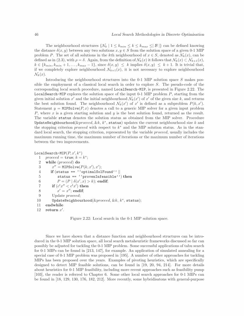
46 Local Search Methodologies in Discrete Optimisation
The neighbourhood structures {Nk | 1 ≤ kmin ≤ k ≤ kmax ≤| B |} can be defined knowingthe distance δ(x, y) between any two solutions x, y ∈ S from the solution space of a given 0-1 MIPproblem P . The set of all solutions in the kth neighbourhood of x ∈ S, denoted as Nk(x), can bedefined as in (2.3), with ρ = δ. Again, from the definition ofNk(x) it follows thatNk(x) ⊂ Nk+1(x),k ∈ {kmin, kmin + 1, . . . , kmax − 1}, since δ(x, y) ≤ k implies δ(x, y) ≤ k + 1. It is trivial that,if we completely explore neighbourhood Nk+1(x), it is not necessary to explore neighbourhoodNk(x).
Introducing the neighbourhood structures into the 0-1 MIP solution space S makes pos-sible the employment of a classical local search in order to explore S. The pseudo-code of thecorresponding local search procedure, named LocalSearch-MIP, is presented in Figure 2.22. TheLocalSearch-MIP explores the solution space of the input 0-1 MIP problem P , starting from thegiven initial solution x′ and the initial neighbourhood Nk(x′) of x′ of the given size k, and returnsthe best solution found. The neighbourhood Nk(x′) of x′ is defined as a subproblem P (k, x′).Statement y = MIPSolve(P, x) denotes a call to a generic MIP solver for a given input problemP , where x is a given starting solution and y is the best solution found, returned as the result.The variable status denotes the solution status as obtained from the MIP solver. ProcedureUpdateNeighbourhood(&proceed, &k, k∗, status) updates the current neighbourhood size k andthe stopping criterion proceed with respect to k∗ and the MIP solution status. As in the stan-dard local search, the stopping criterion, represented by the variable proceed, usually includes themaximum running time, the maximum number of iterations or the maximum number of iterationsbetween the two improvements.
LocalSearch-MIP(P, x′, k∗)1 proceed = true; k = k∗;2 while (proceed) do3 x′′ = MIPSolve(P (k, x′), x′);4 if (status == ‘‘optimalSolFound’’ ||5 status == ‘‘provenInfeasible’’) then6 P = (P | δ(x′, x) > k); endif;7 if (ctx′′ < ctx′) then8 x′ = x′′; endif;9 Update proceed;
10 UpdateNeighbourhood(&proceed, &k, k∗, status);11 endwhile12 return x′.
Figure 2.22: Local search in the 0-1 MIP solution space.
Since we have shown that a distance function and neighbourhood structures can be intro-duced in the 0-1 MIP solution space, all local search metaheuristic frameworks discussed so far canpossibly be adjusted for tackling the 0-1 MIP problem. Some successful applications of tabu searchfor 0-1 MIPs can be found in [213, 147], for example. An application of simulated annealing for aspecial case of 0-1 MIP problem was proposed in [195]. A number of other approaches for tacklingMIPs has been proposed over the years. Examples of pivoting heuristics, which are specificallydesigned to detect MIP feasible solutions, can be found in [19, 20, 94, 214]. For more detailsabout heuristics for 0-1 MIP feasibility, including more recent approaches such as feasibility pump[103], the reader is referred to Chapter 6. Some other local search approaches for 0-1 MIPs canbe found in [18, 129, 130, 176, 182, 212]. More recently, some hybridisatons with general-purpose
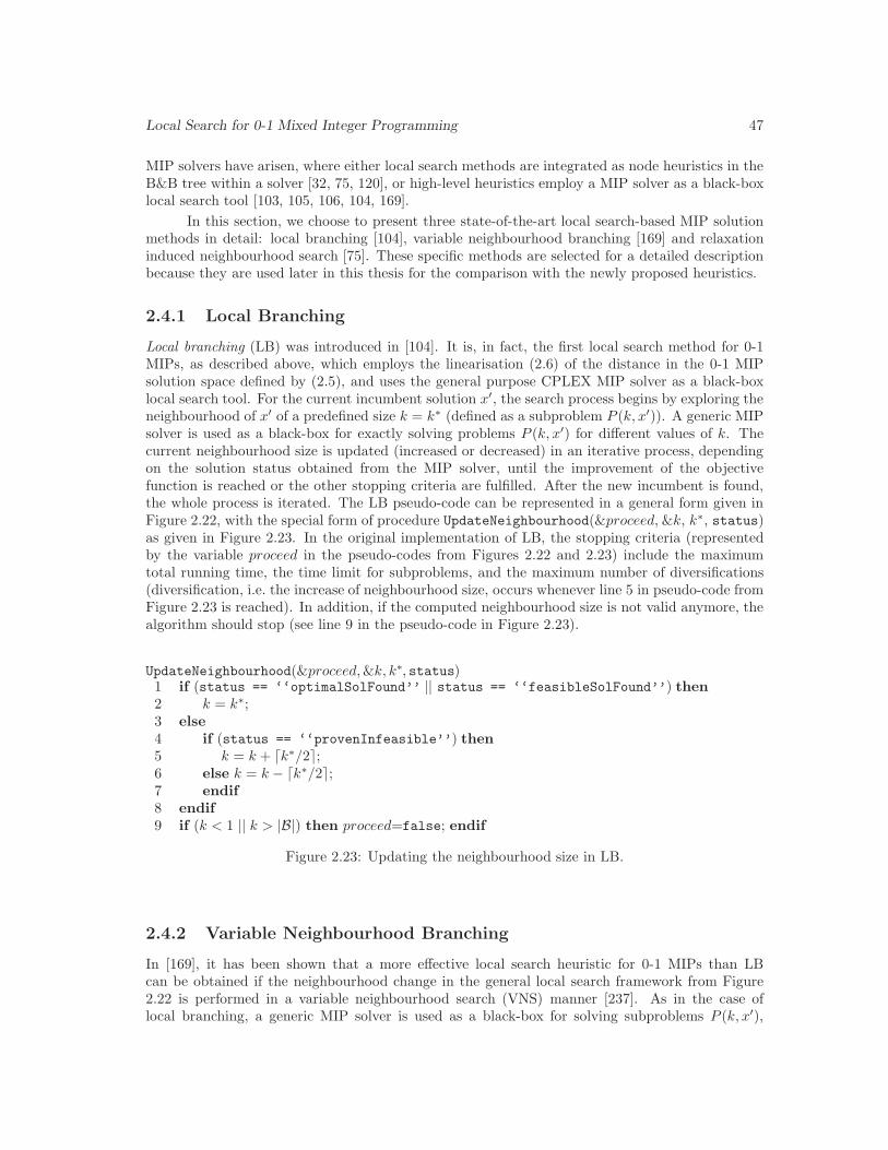
Local Search for 0-1 Mixed Integer Programming 47
MIP solvers have arisen, where either local search methods are integrated as node heuristics in theB&B tree within a solver [32, 75, 120], or high-level heuristics employ a MIP solver as a black-boxlocal search tool [103, 105, 106, 104, 169].
In this section, we choose to present three state-of-the-art local search-based MIP solutionmethods in detail: local branching [104], variable neighbourhood branching [169] and relaxationinduced neighbourhood search [75]. These specific methods are selected for a detailed descriptionbecause they are used later in this thesis for the comparison with the newly proposed heuristics.
2.4.1 Local Branching
Local branching (LB) was introduced in [104]. It is, in fact, the first local search method for 0-1MIPs, as described above, which employs the linearisation (2.6) of the distance in the 0-1 MIPsolution space defined by (2.5), and uses the general purpose CPLEX MIP solver as a black-boxlocal search tool. For the current incumbent solution x′, the search process begins by exploring theneighbourhood of x′ of a predefined size k = k∗ (defined as a subproblem P (k, x′)). A generic MIPsolver is used as a black-box for exactly solving problems P (k, x′) for different values of k. Thecurrent neighbourhood size is updated (increased or decreased) in an iterative process, dependingon the solution status obtained from the MIP solver, until the improvement of the objectivefunction is reached or the other stopping criteria are fulfilled. After the new incumbent is found,the whole process is iterated. The LB pseudo-code can be represented in a general form given inFigure 2.22, with the special form of procedure UpdateNeighbourhood(&proceed, &k, k∗, status)as given in Figure 2.23. In the original implementation of LB, the stopping criteria (representedby the variable proceed in the pseudo-codes from Figures 2.22 and 2.23) include the maximumtotal running time, the time limit for subproblems, and the maximum number of diversifications(diversification, i.e. the increase of neighbourhood size, occurs whenever line 5 in pseudo-code fromFigure 2.23 is reached). In addition, if the computed neighbourhood size is not valid anymore, thealgorithm should stop (see line 9 in the pseudo-code in Figure 2.23).
UpdateNeighbourhood(&proceed, &k, k∗, status)1 if (status == ‘‘optimalSolFound’’ || status == ‘‘feasibleSolFound’’) then2 k = k∗;3 else4 if (status == ‘‘provenInfeasible’’) then5 k = k + ⌈k∗/2⌉;6 else k = k − ⌈k∗/2⌉;7 endif8 endif9 if (k < 1 || k > |B|) then proceed=false; endif
Figure 2.23: Updating the neighbourhood size in LB.
2.4.2 Variable Neighbourhood Branching
In [169], it has been shown that a more effective local search heuristic for 0-1 MIPs than LBcan be obtained if the neighbourhood change in the general local search framework from Figure2.22 is performed in a variable neighbourhood search (VNS) manner [237]. As in the case oflocal branching, a generic MIP solver is used as a black-box for solving subproblems P (k, x′),

48 Local Search Methodologies in Discrete Optimisation
i.e. neighbourhood exploration. Since neighbourhoods are explored completely, the resulting searchmethod is a deterministic variant of VNS, so called variable neighbourhood descent (VND) (see[162] and Section 2.3 in Chapter 2). The pseudo-code of VND for MIPs, called VND-MIP, canalso be represented in a general form given in Figure 2.22, but with the special form of procedureUpdateNeighbourhood(&proceed, &k, k∗, status) as given in Figure 2.24.
UpdateNeighbourhood(&proceed, &k, k∗, status)1 if (status == ‘‘optimalSolFound’’ || status == ‘‘feasibleSolFound’’) then2 k = 1;3 else4 if (status == ‘‘provenInfeasible’’) then5 k = k + 1;6 else proceed = false;7 endif8 endif9 if (k > k∗) then proceed=false; endif
Figure 2.24: Neighbourhood update in VND-MIP.
Note that parameter k∗ in VND-MIP represents the maximum allowed neighbourhood size, whereasin LB it represents the initial neighbourhood size for a given incumbent solution vector.
VND-MIP can be extended to a general VNS scheme for 0-1 MIPs if a diversification mech-anism (shaking step in general VNS, see [237] and Section 2.3 in Chapter 2) is added. This GVNSscheme for 0-1 MIPs, called variable neighbourhood branching (VNB) was proposed in [169]. Thediversification (shaking) in VNB implies choosing a new incumbent solution each time VND-MIPfails to improve the current incumbent and reiterating the whole search process starting from thatnew point. This can be performed by choosing the first feasible solution from the disk of radii kand k + kstep, where k is the current neighbourhood size, and kstep is a given input parameter.The disk size can then be increased as long as the feasible solution is not found. The pseudo-codeof the shaking procedure is given in Figure 2.25.
Procedure Shake(P, x∗, &k, kstep, kmax)1 Choose stopping criterion (set proceed = true);2 Set solutionLimit = 1; Set x′ = x∗;3 while (proceed && k ≤ kmax) do4 Q = (P | k ≤ δ(B, x∗, x) ≤ k + kstep);5 x′ = MIPSolve(Q, x∗, solutionLimit);6 if (solutionStatus == proven infeasible ||
solutionStatus == no feasible found) then7 k = k + kstep; // Next neighbourhood.
8 Update proceed;9 else proceed = false;10 endwhile11 Reset solutionLimit = ∞; return x′;
Figure 2.25: VNB shaking pseudo-code.
The complete pseudo-code of the VNB procedure is given in Figure 2.26. The input param-eters of VNB are the minimum neighbourhood size kmin, the neighbourhood size increment step
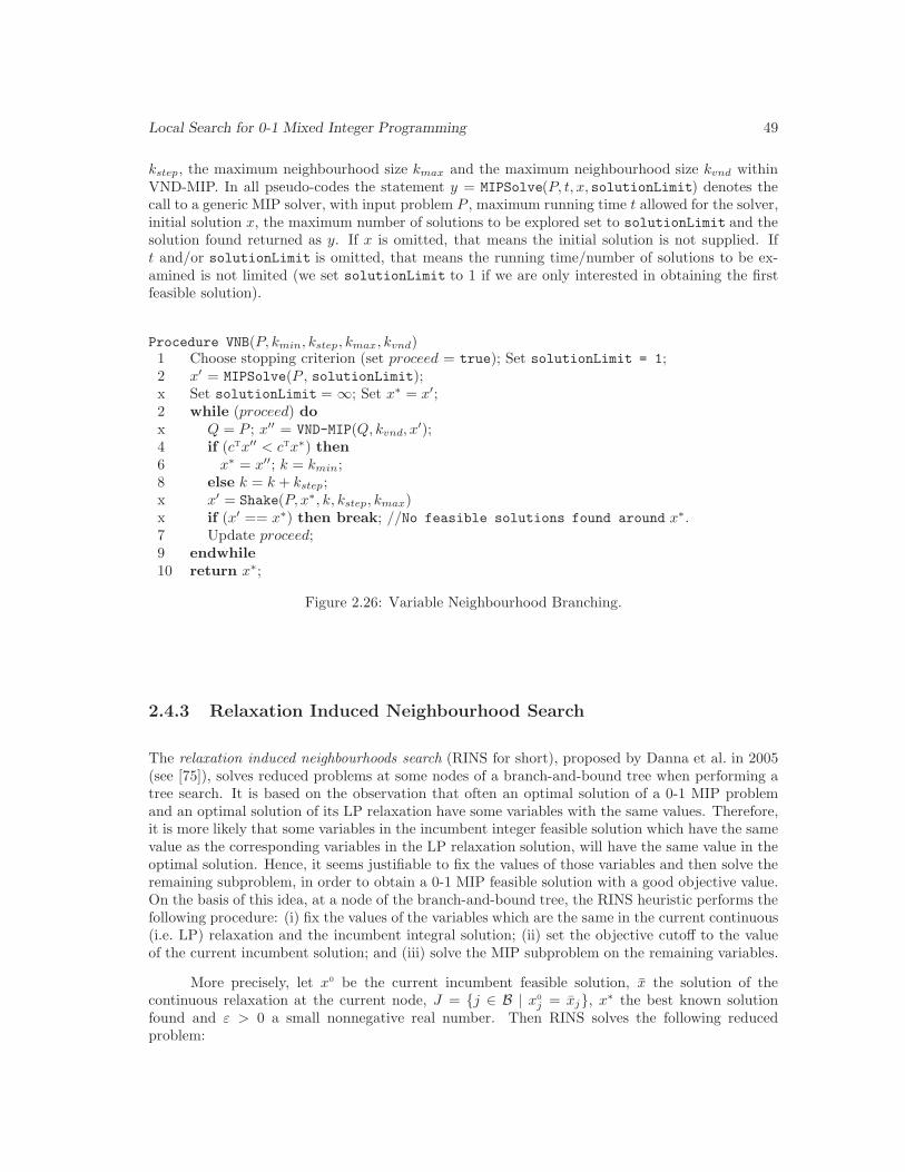
Local Search for 0-1 Mixed Integer Programming 49
kstep, the maximum neighbourhood size kmax and the maximum neighbourhood size kvnd withinVND-MIP. In all pseudo-codes the statement y = MIPSolve(P, t, x, solutionLimit) denotes thecall to a generic MIP solver, with input problem P , maximum running time t allowed for the solver,initial solution x, the maximum number of solutions to be explored set to solutionLimit and thesolution found returned as y. If x is omitted, that means the initial solution is not supplied. Ift and/or solutionLimit is omitted, that means the running time/number of solutions to be ex-amined is not limited (we set solutionLimit to 1 if we are only interested in obtaining the firstfeasible solution).
Procedure VNB(P, kmin, kstep, kmax, kvnd)1 Choose stopping criterion (set proceed = true); Set solutionLimit = 1;2 x′ = MIPSolve(P , solutionLimit);x Set solutionLimit = ∞; Set x∗ = x′;2 while (proceed) dox Q = P ; x′′ = VND-MIP(Q, kvnd, x
′);4 if (ctx′′ < ctx∗) then6 x∗ = x′′; k = kmin;8 else k = k + kstep;x x′ = Shake(P, x∗, k, kstep, kmax)x if (x′ == x∗) then break; //No feasible solutions found around x∗.7 Update proceed;9 endwhile10 return x∗;
Figure 2.26: Variable Neighbourhood Branching.
2.4.3 Relaxation Induced Neighbourhood Search
The relaxation induced neighbourhoods search (RINS for short), proposed by Danna et al. in 2005(see [75]), solves reduced problems at some nodes of a branch-and-bound tree when performing atree search. It is based on the observation that often an optimal solution of a 0-1 MIP problemand an optimal solution of its LP relaxation have some variables with the same values. Therefore,it is more likely that some variables in the incumbent integer feasible solution which have the samevalue as the corresponding variables in the LP relaxation solution, will have the same value in theoptimal solution. Hence, it seems justifiable to fix the values of those variables and then solve theremaining subproblem, in order to obtain a 0-1 MIP feasible solution with a good objective value.On the basis of this idea, at a node of the branch-and-bound tree, the RINS heuristic performs thefollowing procedure: (i) fix the values of the variables which are the same in the current continuous(i.e. LP) relaxation and the incumbent integral solution; (ii) set the objective cutoff to the valueof the current incumbent solution; and (iii) solve the MIP subproblem on the remaining variables.
More precisely, let x0 be the current incumbent feasible solution, x the solution of thecontinuous relaxation at the current node, J = {j ∈ B | x0
j = xj}, x∗ the best known solutionfound and ε > 0 a small nonnegative real number. Then RINS solves the following reducedproblem:

50 Local Search Methodologies in Discrete Optimisation
(2.17) P (x0, x∗, J)
min ctxs.t. Ax ≥ b
xj = x0
j ∀j ∈ Jctx ≤ ctx∗ − εxj ∈ {0, 1} ∀j ∈ B 6= ∅xj ≥ 0 ∀j ∈ C
2.5 Future Trends: the Hyper-reactive Optimisation
The future developments in metaheuristics are likely to evolve in some of the following directions:1) hybridisation/cooperation, 2) parallelisation, 3) adaptive memory integration, 4) dynamic ad-justment of components during the search, 5) different combinations of 1), 2), 3) and 4), etc.
In my view, automatic component tuning, together with adaptive memory integration, seemsto be particularly auspicious in order to change the behaviour of the search process, which maydepend on the search stage and search history. Note that the best performance is expected if notonly the basic parameters of a particular method are considered, but also the different problemformulations and possible neighbourhood structures are included. This “all-inclusive” approachwill be referred to as hyper-reactive search in the following text. The motivation for the namecomes from the term “hyper-heuristics”, which refers to methods which explore the search spacecomprised of heuristic methods for a particular optimisation problem (rather than the search spaceof the optimisation problem) and the term “reactive search”, which refers to an automated tuningof parameters during the search process (see, for example, [13, 22, 23, 44, 227, 255]).
Indeed, any standard local search-based metaheuristic is defined by the search operatorSearch (a set of algorithmic rules for determining the next candidate solution, normally different inmetaheuristic frameworks: simulated annealing, tabu search, variable neighbourhood search, etc.),the set of possible problem formulations F (most metahuristics operate on a single formulation), theset of possible initial solutions X , possible sets of neighbourhood structures N, and the set Π of allpossible method-specific parameters. Therefore, a standard local search-based metaheuristic can beviewed as a 5-tuple (Search,F , X,N, Π), with a general pseudo-code as in Figure 2.27. By choosingparticular values for each of the five components from (Search,F , X,N, Π), a particular heuristicfor a specific optimisation problem is obtained. More precisely, by choosing a specific searchoperator Search(defined by some local search metaheuristic), a specific problem formulation φ ∈ F ,a specific initial solution x ∈ X , a set of neighbourhood structures {Nk | 1 ≤ kmin ≤ k ≤ kmax} ⊆N, and specific values v1, v2, . . . , vℓ of parameters π1, π2, . . . , πℓ, ℓ ≤ |Π|, {π1, π2, . . . , πℓ} ⊆ Π, aproblem-specific heuristic is obtained, for the optimisation problem P formulated by φ, with x asthe initial solution. This way, one can observe that each metaheuristic generates a set of problem-specific heuristics. In a hyper-reactive approach, different heuristics from this set are chosen totackle the input optimisation problem in the different stages of the search process. Therefore, thehyper-reactive search can be viewed as a special type of a hyper-heuristic method (and hence thefirst part of the word “hyper-reactive”). The general framework of the hyper-reactive search can berepresented as in Figure 2.28, where Sφ is the solution space of the input problem P in formulationφ.
Obviously, a hyper-reactive approach can be integrated into any local search-based meta-heuristic. An example of a hyper-reactive VNS, called HR-VNS, is provided in Figure 2.29. Usually,
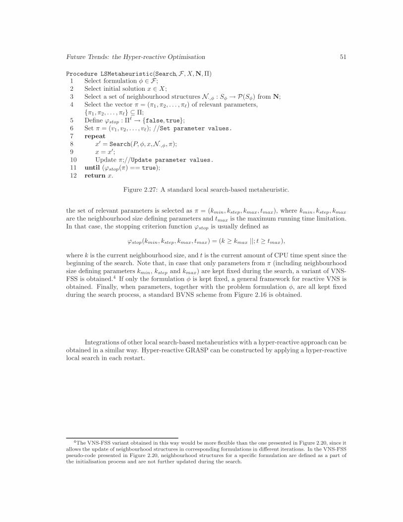
Future Trends: the Hyper-reactive Optimisation 51
Procedure LSMetaheuristic(Search,F , X,N, Π)1 Select formulation φ ∈ F ;2 Select initial solution x ∈ X ;3 Select a set of neighbourhood structures N·,φ : Sφ → P(Sφ) from N;4 Select the vector π = (π1, π2, . . . , πℓ) of relevant parameters,
{π1, π2, . . . , πℓ} ⊆ Π;5 Define ϕstop : Πℓ → {false, true};6 Set π = (v1, v2, . . . , vℓ); //Set parameter values.
7 repeat8 x′ = Search(P, φ, x,N·,φ, π);9 x = x′;10 Update π;//Update parameter values.
11 until (ϕstop(π) == true);12 return x.
Figure 2.27: A standard local search-based metaheuristic.
the set of relevant parameters is selected as π = (kmin, kstep, kmax, tmax), where kmin, kstep, kmax
are the neighbourhood size defining parameters and tmax is the maximum running time limitation.In that case, the stopping criterion function ϕstop is usually defined as
ϕstop(kmin, kstep, kmax, tmax) = (k ≥ kmax ||; t ≥ tmax),
where k is the current neighbourhood size, and t is the current amount of CPU time spent since thebeginning of the search. Note that, in case that only parameters from π (including neighbourhoodsize defining parameters kmin, kstep and kmax) are kept fixed during the search, a variant of VNS-FSS is obtained.4 If only the formulation φ is kept fixed, a general framework for reactive VNS isobtained. Finally, when parameters, together with the problem formulation φ, are all kept fixedduring the search process, a standard BVNS scheme from Figure 2.16 is obtained.
Integrations of other local search-based metaheuristics with a hyper-reactive approach can beobtained in a similar way. Hyper-reactive GRASP can be constructed by applying a hyper-reactivelocal search in each restart.
4The VNS-FSS variant obtained in this way would be more flexible than the one presented in Figure 2.20, since itallows the update of neighbourhood structures in corresponding formulations in different iterations. In the VNS-FSSpseudo-code presented in Figure 2.20, neighbourhood structures for a specific formulation are defined as a part ofthe initialisation process and are not further updated during the search.
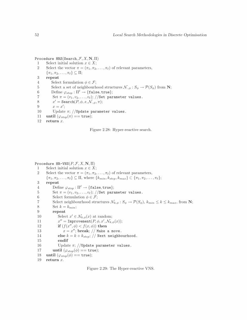
52 Local Search Methodologies in Discrete Optimisation
Procedure HRS(Search,F , X,N, Π)1 Select initial solution x ∈ X ;2 Select the vector π = (π1, π2, . . . , πℓ) of relevant parameters,
{π1, π2, . . . , πℓ} ⊆ Π;3 repeat4 Select formulation φ ∈ F ;5 Select a set of neighbourhood structures N·,φ : Sφ → P(Sφ) from N;6 Define ϕstop : Πℓ → {false, true};7 Set π = (v1, v2, . . . , vℓ); //Set parameter values.
8 x′ = Search(P, φ, x,N·,φ, π);9 x = x′;10 Update π; //Update parameter values.
11 until (ϕstop(π) == true);12 return x.
Figure 2.28: Hyper-reactive search.
Procedure HR-VNS(P,F , X,N, Π)1 Select initial solution x ∈ X ;2 Select the vector π = (π1, π2, . . . , πℓ) of relevant parameters,
{π1, π2, . . . , πℓ} ⊆ Π, where {kmin, kstep, kmax} ⊂ {π1, π2, . . . , πℓ};3 repeat4 Define ϕstop : Πℓ → {false, true};5 Set π = (v1, v2, . . . , vℓ); //Set parameter values.
6 Select formulation φ ∈ F ;7 Select neighbourhood structures Nk,φ : Sφ → P(Sφ), kmin ≤ k ≤ kmax, from N;8 Set k = kmin;9 repeat10 Select x′ ∈ Nk,φ(x) at random;11 x′′ = Improvement(P, φ, x′,Nk,φ(x));12 if (f(x′′, φ) < f(x, φ)) then13 x = x′′; break; // Make a move.
14 else k = k + kstep; // Next neighbourhood.
15 endif16 Update π; //Update parameter values.
17 until (ϕstop(φ) == true);18 until (ϕstop(φ) == true);19 return x.
Figure 2.29: The Hyper-reactive VNS.

Chapter 3
Variable Neighbourhood Searchfor Colour Image Quantisation
Colour image quantisation (or CIQ for short) is a data compression technique that reduces thetotal number of colours in an image’s colour space, thus depicting the original image with a limitednumber of representative colours [170]. A true colour image is normally represented by a matrix ofpixel colours, each consisting of 24 bits – one byte for red, one byte for green and one byte for bluecomponent1. However, it is often the case that only 256 (of 224 ≈ 16.8 million possible) colourscan be displayed on a certain display device. Hence, it is necessary that images be quantised to8 bits in order to be represented in these devices. In addition, the decrease of colour informationimplies a reduction of the image size and is therefore associated with data compression. Thisgreatly reduces the task of transmitting images.
Given an original N -colour image, the quantiser first determines a set of M representativecolours – a colourmap, then assigns to each colour in the original image its representative colourin the colourmap, and finally redraws the image by substituting the original colour in every pixelwith the value previously assigned to it. It is not hard to see that the quantiser actually performsa clustering of the image’s colour space into M desired clusters and maps each point of the colourspace to its representative cluster colour (i.e. cluster centroid or median). The final objective ofcolour image quantisation is to minimize the difference between the reproduced M -colour imageand the original N -colour image, i.e., to find an optimal solution to a colour space clusteringproblem. The difference is usually represented by the mean square error (MSE criterion); it willbe formally defined later in the text.
Therefore CIQ problem may be modelled as a clustering problem. More formally, an imageI can be considered as a function I : S → R3, S ⊂ Z × Z, with each dimension of the setI(S) = {I(x) | x ∈ S} representing one of the red, green and blue components of the pixel’s colour,respectively, and having an integer value between 0 and 255. The range C = I(S), C ⊂ R3, offunction I defines the colour space of I. Clearly, colour quantisation of I consists of solving theclustering problem for its colour space C and a given number of colours M , thus obtaining theclusters C1, C2, . . . , CM , and then replacing the colour I(x) of each pixel x ∈ S with the centroidof it’s associated cluster Ci.
1This representation of pixel colours in a true colour image is known as the RGB (red, green, blue) colour model.A number of other colour models exist in which colour image quantisation can be performed. Nevertheless, themethod discussed here and the results reported later are all based on the RGB model. This method, however, couldbe easily implemented in any other colour model.
53
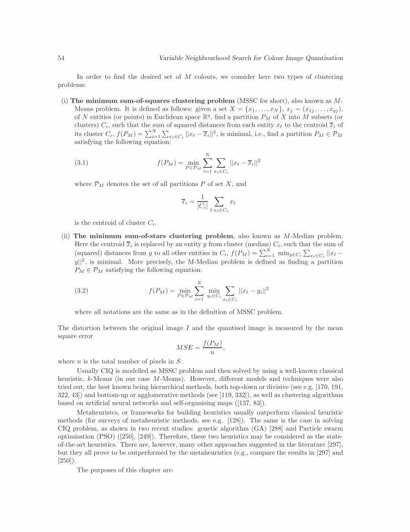
54 Variable Neighbourhood Search for Colour Image Quantisation
In order to find the desired set of M colours, we consider here two types of clusteringproblems:
(i) The minimum sum-of-squares clustering problem (MSSC for short), also known as M -Means problem. It is defined as follows: given a set X = {x1, . . . , xN}, xj = (x1j , . . . , xqj),of N entities (or points) in Euclidean space Rq, find a partition PM of X into M subsets (orclusters) Ci, such that the sum of squared distances from each entity xℓ to the centroid xi of
its cluster Ci, f(PM ) =∑N
i=1
∑xℓ∈Ci
||xℓ − xi||2, is minimal, i.e., find a partition PM ∈ PM
satisfying the following equation:
(3.1) f(PM ) = minP∈PM
N∑
i=1
∑
xℓ∈Ci
||xℓ − xi||2
where PM denotes the set of all partitions P of set X , and
xi =1
|Ci|
∑
ℓ:xℓ∈Ci
xℓ
is the centroid of cluster Ci.
(ii) The minimum sum-of-stars clustering problem, also known as M -Median problem.Here the centroid xi is replaced by an entity y from cluster (median) Ci, such that the sum of
(squared) distances from y to all other entities in Ci, f(PM ) =∑N
i=1 miny∈Ci
∑xℓ∈Ci
||xℓ −
y||2, is minimal. More precisely, the M-Median problem is defined as finding a partitionPM ∈ PM satisfying the following equation:
(3.2) f(PM ) = minP∈PM
N∑
i=1
minyi∈Ci
∑
xℓ∈Ci
||xℓ − yi||2
where all notations are the same as in the definition of MSSC problem.
The distortion between the original image I and the quantised image is measured by the meansquare error
MSE =f(PM )
n,
where n is the total number of pixels in S.
Usually CIQ is modelled as MSSC problem and then solved by using a well-known classicalheuristic, k-Means (in our case M -Means). However, different models and techniques were alsotried out, the best known being hierarchical methods, both top-down or divisive (see e.g. [170, 191,322, 43]) and bottom-up or agglomerative methods (see [119, 332]), as well as clustering algorithmsbased on artificial neural networks and self-organising maps ([137, 83]).
Metaheuristcs, or frameworks for building heuristics usually outperform classical heuristicmethods (for surveys of metaheuristic methods, see e.g. [128]). The same is the case in solvingCIQ problem, as shown in two recent studies: genetic algorithm (GA) [288] and Particle swarmoptimisation (PSO) ([250], [249]). Therefore, these two heuristics may be considered as the state-of-the-art heuristics. There are, however, many other approaches suggested in the literature [297],but they all prove to be outperformed by the metaheuristics (e.g., compare the results in [297] and[250]).
The purposes of this chapter are:
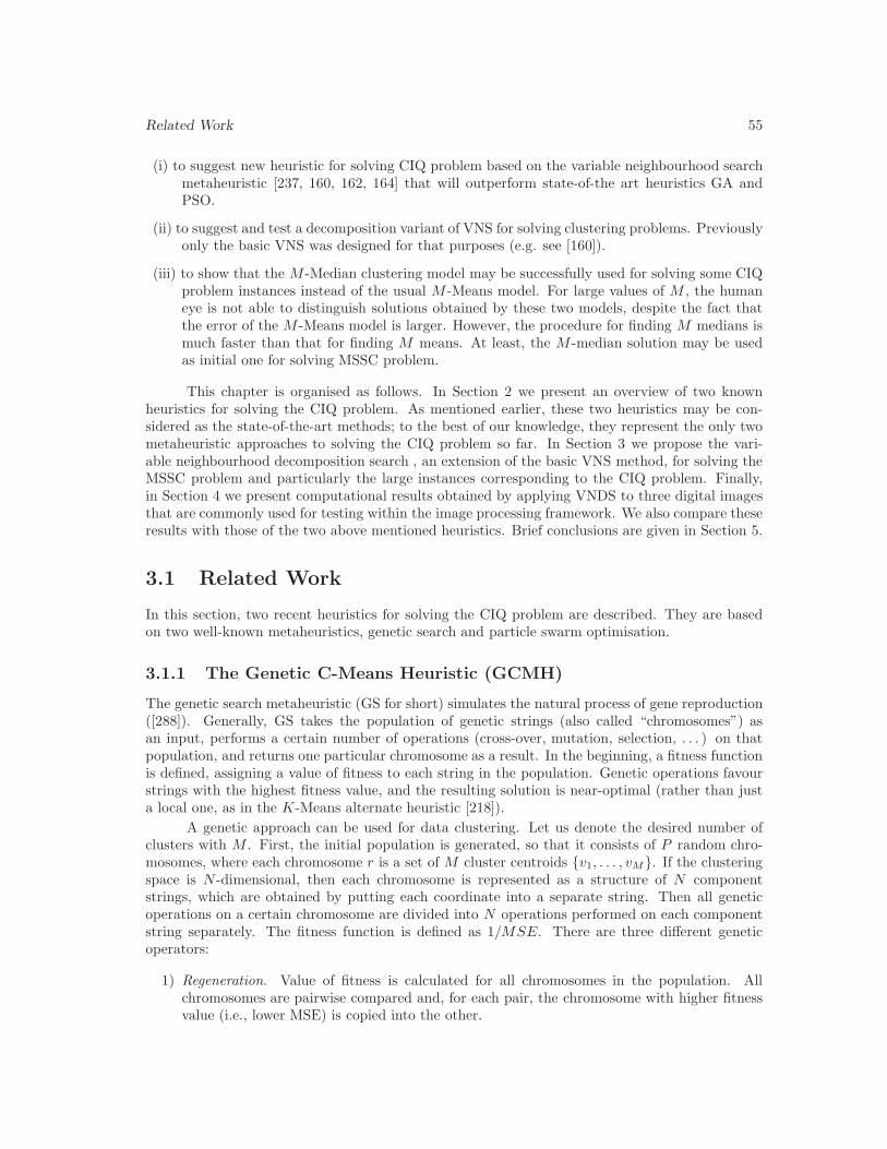
Related Work 55
(i) to suggest new heuristic for solving CIQ problem based on the variable neighbourhood searchmetaheuristic [237, 160, 162, 164] that will outperform state-of-the art heuristics GA andPSO.
(ii) to suggest and test a decomposition variant of VNS for solving clustering problems. Previouslyonly the basic VNS was designed for that purposes (e.g. see [160]).
(iii) to show that the M -Median clustering model may be successfully used for solving some CIQproblem instances instead of the usual M -Means model. For large values of M , the humaneye is not able to distinguish solutions obtained by these two models, despite the fact thatthe error of the M -Means model is larger. However, the procedure for finding M medians ismuch faster than that for finding M means. At least, the M -median solution may be usedas initial one for solving MSSC problem.
This chapter is organised as follows. In Section 2 we present an overview of two knownheuristics for solving the CIQ problem. As mentioned earlier, these two heuristics may be con-sidered as the state-of-the-art methods; to the best of our knowledge, they represent the only twometaheuristic approaches to solving the CIQ problem so far. In Section 3 we propose the vari-able neighbourhood decomposition search , an extension of the basic VNS method, for solving theMSSC problem and particularly the large instances corresponding to the CIQ problem. Finally,in Section 4 we present computational results obtained by applying VNDS to three digital imagesthat are commonly used for testing within the image processing framework. We also compare theseresults with those of the two above mentioned heuristics. Brief conclusions are given in Section 5.
3.1 Related Work
In this section, two recent heuristics for solving the CIQ problem are described. They are basedon two well-known metaheuristics, genetic search and particle swarm optimisation.
3.1.1 The Genetic C-Means Heuristic (GCMH)
The genetic search metaheuristic (GS for short) simulates the natural process of gene reproduction([288]). Generally, GS takes the population of genetic strings (also called “chromosomes”) asan input, performs a certain number of operations (cross-over, mutation, selection, . . . ) on thatpopulation, and returns one particular chromosome as a result. In the beginning, a fitness functionis defined, assigning a value of fitness to each string in the population. Genetic operations favourstrings with the highest fitness value, and the resulting solution is near-optimal (rather than justa local one, as in the K-Means alternate heuristic [218]).
A genetic approach can be used for data clustering. Let us denote the desired number ofclusters with M . First, the initial population is generated, so that it consists of P random chro-mosomes, where each chromosome r is a set of M cluster centroids {v1, . . . , vM}. If the clusteringspace is N -dimensional, then each chromosome is represented as a structure of N componentstrings, which are obtained by putting each coordinate into a separate string. Then all geneticoperations on a certain chromosome are divided into N operations performed on each componentstring separately. The fitness function is defined as 1/MSE. There are three different geneticoperators:
1) Regeneration. Value of fitness is calculated for all chromosomes in the population. Allchromosomes are pairwise compared and, for each pair, the chromosome with higher fitnessvalue (i.e., lower MSE) is copied into the other.
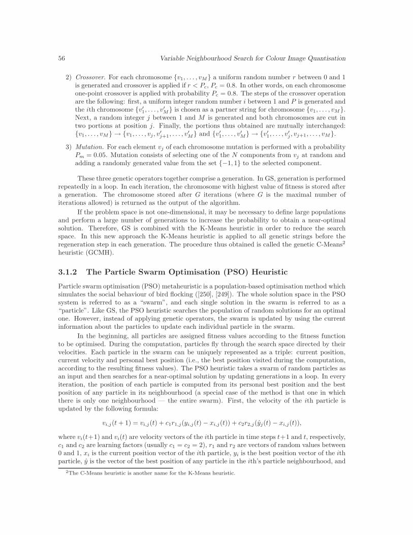
56 Variable Neighbourhood Search for Colour Image Quantisation
2) Crossover. For each chromosome {v1, . . . , vM} a uniform random number r between 0 and 1is generated and crossover is applied if r < Pc, Pc = 0.8. In other words, on each chromosomeone-point crossover is applied with probability Pc = 0.8. The steps of the crossover operationare the following: first, a uniform integer random number i between 1 and P is generated andthe ith chromosome {v′1, . . . , v
′M} is chosen as a partner string for chromosome {v1, . . . , vM}.
Next, a random integer j between 1 and M is generated and both chromosomes are cut intwo portions at position j. Finally, the portions thus obtained are mutually interchanged:{v1, . . . , vM} → {v1, . . . , vj , v
′j+1, . . . , v
′M} and {v′1, . . . , v
′M} → {v
′1, . . . , v
′j , vj+1, . . . , vM}.
3) Mutation. For each element vj of each chromosome mutation is performed with a probabilityPm = 0.05. Mutation consists of selecting one of the N components from vj at random andadding a randomly generated value from the set {−1, 1} to the selected component.
These three genetic operators together comprise a generation. In GS, generation is performedrepeatedly in a loop. In each iteration, the chromosome with highest value of fitness is stored aftera generation. The chromosome stored after G iterations (where G is the maximal number ofiterations allowed) is returned as the output of the algorithm.
If the problem space is not one-dimensional, it may be necessary to define large populationsand perform a large number of generations to increase the probability to obtain a near-optimalsolution. Therefore, GS is combined with the K-Means heuristic in order to reduce the searchspace. In this new approach the K-Means heuristic is applied to all genetic strings before theregeneration step in each generation. The procedure thus obtained is called the genetic C-Means2
heuristic (GCMH).
3.1.2 The Particle Swarm Optimisation (PSO) Heuristic
Particle swarm optimisation (PSO) metaheuristic is a population-based optimisation method whichsimulates the social behaviour of bird flocking ([250], [249]). The whole solution space in the PSOsystem is referred to as a “swarm”, and each single solution in the swarm is referred to as a“particle”. Like GS, the PSO heuristic searches the population of random solutions for an optimalone. However, instead of applying genetic operators, the swarm is updated by using the currentinformation about the particles to update each individual particle in the swarm.
In the beginning, all particles are assigned fitness values according to the fitness functionto be optimised. During the computation, particles fly through the search space directed by theirvelocities. Each particle in the swarm can be uniquely represented as a triple: current position,current velocity and personal best position (i.e., the best position visited during the computation,according to the resulting fitness values). The PSO heuristic takes a swarm of random particles asan input and then searches for a near-optimal solution by updating generations in a loop. In everyiteration, the position of each particle is computed from its personal best position and the bestposition of any particle in its neighbourhood (a special case of the method is that one in whichthere is only one neighbourhood — the entire swarm). First, the velocity of the ith particle isupdated by the following formula:
vi,j(t + 1) = vi,j(t) + c1r1,j(yi,j(t)− xi,j(t)) + c2r2,j(yj(t)− xi,j(t)),
where vi(t+1) and vi(t) are velocity vectors of the ith particle in time steps t+1 and t, respectively,c1 and c2 are learning factors (usually c1 = c2 = 2), r1 and r2 are vectors of random values between0 and 1, xi is the current position vector of the ith particle, yi is the best position vector of the ithparticle, y is the vector of the best position of any particle in the ith’s particle neighbourhood, and
2The C-Means heuristic is another name for the K-Means heuristic.
VNS Methods for the CIQ Problem 57
index j denotes the current dimension. Then the following formula is used to update the positionof the ith particle: xi(t + 1) = xi(t) + vi(t + 1). The loop is run until the maximum number ofiterations allowed or minimum error criteria is attained.
The main difference between GS and PSO is in the information sharing mechanism. Whilein GS all chromosomes share information with each other, in PSO there is just one particle (theone with the best visited position) that sends the information to the rest of the swarm. Thereforeall particles tend to converge to the optimal solution quickly, whereas in GS the whole populationas a single group moves towards an optimal area, which results in slower performance comparedto PSO.
3.2 VNS Methods for the CIQ Problem
In this section several new variants of variable neighbourhood search for the CIQ problem are pro-posed. Two different VNS schemes are exploited and combined: variable neighbourhood decom-position search (VNDS) [168] and reduced variable neighbourhood search (RVNS) [159]. Variableneighbourhood decomposition search is an extension of VNS that searches the problem space bydecomposing it into smaller size subspaces. The improved solution found in a given subspace isthen extended to a corresponding solution of the whole problem (see Chapter 2, Section 2.3 formore details). In this section, we describe a new VNDS-based technique for colour image quantisa-tion. Moreover, this technique can also be viewed as a new approach to tackling the more generalMSSC problem. It is particularly well-suited for solving very large problem instances. Reducedvariable neighbourhood search is a stochastic variant of VNS, where new candidate solutions arechosen at random from appropriate neighbourhoods (see Chapter 2, Section 2.3). In this chaptersome new CIQ techniques are developed based on the RVNS framework. The integration of RVNSwithin a general VNDS scheme is also studied.
The CIQ problem space is the set of all colour triplets present in the image to be quantised.Although our quantisation technique is not restricted to 8-bit quantisation, we assume that theRGB coordinates of each colour triplet are integers between 0 and 255 (it is possible to derive otherimplementations of our technique that do not satisfy this assumption). Since our problem spaceis a subset of Z3, we use the VNS methods adjusted for solving the M-Median problem. In otherwords, medians are always chosen to be some of the colour triplets from the original image. Thepoints that coincide with centroids are referred to as “occupied” points, whereas all other pointsare referred to as “unoccupied” points. The MSE is used as the objective function. In the end,the solution obtained by VNDS is refined by applying the K-Means algorithm and rounding offthe real components of the resulting triplets.
Let us denote with n the total number of pixels in the image to be quantised and with M thedesired number of colours in the colourmap, i.e., the number of clusters of the colour space. Theheuristic first initializes cluster centroids by randomly selecting M colour triplets from the colourspace of the given image. All the remaining colour triplets are then assigned to their closest centroid(in terms of squared Euclidean distance) to form clusters of the image’s colour space. The reducedVNS method (which will be explained in more details further in the text) is applied to this solutiononce and the resulting solution is used as the initial solution for the VNDS algorithm. The set ofneighbourhood structures in the CIQ framework is defined so that any k ≤ M centroids from thecurrent solution, together with their associated points, represent a point in the kth neighbourhoodNk of the current solution. After generating the initial solution, the VNDS algorithm repeatedlyperforms the following actions until the stopping criterion is met: selecting a point from Nk atrandom (starting with k = 1), solving the corresponding subproblem by some local search method(in our case the reduced VNS heuristic), extending the so-obtained solution to the corresponding

58 Variable Neighbourhood Search for Colour Image Quantisation
solution in the whole problem space (i.e., adding the centroids outside Nk and their associatedpoints) and either moving to the new solution if it is better than the incumbent and continuingthe search in its first neighbourhood, or moving to the next neighbourhood of the current solutionotherwise. The heuristic stops if a maximal number of iterations between two improvements or amaximal total number of iterations allowed is reached.
Since the subproblem solving method used in our implementation of VNDS heuristic isanother VNS scheme — the so-called reduced VNS (RVNS) method, we will first provide theoutline of the RVNS algorithm. It is based on the so-called J-Means (or Jump Means) heuristicfor solving the MSSC problem [160, 26]: the neighbourhood of a current solution PM is defined asall possible “centroid to entity re-locations” (not “entity to cluster re-allocations”), so that afterthe jump move, many entities (colours) change their cluster. Thus, the jump in re-allocation typeof neighbourhood is performed.
Several variants of J-Means heuristic have been analysed in [160, 26]. After performing thejump move, the questions are: (i) whether and when the solution will be improved by alternate orK-Means heuristic? (ii) how many iterations of K-Means to perform? If K-Means is used always,and until the end, then the final procedure will be time consuming. Since CIQ problem instancesare usually huge, we decide to apply the full K-Means only once, in the end of our VNDS. Forthe same reason, we use RVNS (instead of the basic VNS) within the decomposition. In that way,RVNS is used to create a set of M representative colours among the already existing colours ofthe image. In other words, we apply RVNS for solving M-Median problem (3.2), not M-Meansproblem (3.1). The steps of the RVNS algorithm are presented in Figure 3.1.
Initialisation. Set value iRVNS for the maximal number of iterations allowed betweentwo improvements. Set current iteration’s counter: i = 0 and the indicator of iterationin which optimal solution was found: ibest = i.Main step.Repeat the following sequence(1) k = 1;(2) Repeat the following steps
(a) i = i + 1;(b) Shaking (J-Means moves).
for j = 1 to k doi) Select one of the unoccupied points from the current solution PM
at random; denote the selected point with xadd and add it as anew cluster centroid.
ii) Find index del of the best centroid deletion.iii) Replace centroid xdel by xadd and update assignments and ob-
jective function accordingly. Denote the so-obtained solution andobjective function value with P ′M and f ′, respectively.
endfor(c) Neighbourhood change. If this solution is better than the incumbent (f ′ <
fopt), move there (PM = P ′M , fopt = f ′ and ibest = i) and go to step (1);otherwise, continue the search in the next neighbourhood (k = k + 1) of thecurrent solution;
until k = kmax or i− ibest = iRVNS
until i− ibest = iRVNS
Figure 3.1: RVNS for CIQ.
It is easy to see that the RVNS method is obtained from the basic VNS algorithm if we do
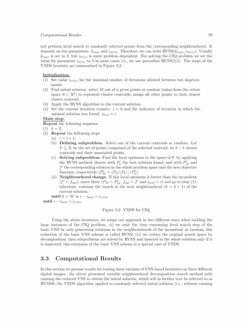
Computational Results 59
not perform local search to randomly selected points from the corresponding neighbourhood. Itdepends on two parameters: kmax and iRVNS. Therefore, we can write RVNS(kmax, iRVNS). Usuallykmax is set to 2, but iRVNS is more problem dependent. For solving the CIQ problem we set thevalue for parameter iRVNS to 5 in most cases, i.e., we use procedure RVNS(2,5). The steps of theVNDS heuristic are summarised in Figure 3.2.
Initialisation.(1) Set value iVNDS for the maximal number of iterations allowed between two improve-
ments.(2) Find initial solution: select M out of n given points at random (taken from the colour
space S ⊂ R3) to represent cluster centroids; assign all other points to their closestcluster centroid.
(3) Apply the RVNS algorithm to the current solution.(4) Set the current iteration counter: i = 0 and the indicator of iteration in which the
optimal solution was found: ibest = i.Main step.Repeat the following sequence(1) k = 2;(2) Repeat the following steps
(a) i = i + 1;(b) Defining subproblem. Select one of the current centroids at random. Let
Y ⊆ X be the set of points comprised of the selected centroid, its k− 1 closestcentroids and their associated points.
(c) Solving subproblem. Find the local optimum in the space of Y by applyingthe RVNS method; denote with P ′k the best solution found, and with P ′M andf ′ the corresponding solution in the whole problem space and the new objectivefunction, respectively (P ′M = (PM\Pk) ∪ P ′k).
(d) Neighbourhood change. If this local optimum is better than the incumbent(f ′ < fopt), move there (PM = P ′M , fopt = f ′ and ibest = i) and go to step (1);otherwise, continue the search in the next neighbourhood (k = k + 1) of thecurrent solution.
until k = M or i− ibest = iVNDS
until i− ibest = iVNDS
Figure 3.2: VNDS for CIQ.
Using the above heuristics, we adapt our approach in two different ways when tackling thelarge instances of the CIQ problem: (i) we omit the time consuming local search step of thebasic VNS by only generating solutions in the neighbourhoods of the incumbent at random; thisreduction of the basic VNS scheme is called RVNS; (ii) we reduce the original search space bydecomposition; then subproblems are solved by RVNS and inserted in the whole solution only if itis improved; this extension of the basic VNS scheme is a special case of VNDS.
3.3 Computational Results
In this section we present results for testing three variants of VNS-based heuristics on three differentdigital images: the above presented variable neighbourhood decomposition search method withrunning the reduced VNS to obtain the initial solution, which will in further text be referred to asRVNDS; the VNDS algorithm applied to randomly selected initial solution (i.e., without running

60 Variable Neighbourhood Search for Colour Image Quantisation
the RVNS in step (3) of Initialisation), which will in further text be referred to as VNDS; andthe RVNS heuristic alone, without performing the decomposition before running the K-Meansalgorithm.
The RVNDS, VNDS and RVNS heuristics are compared with the GCMH and PSO heuris-tics with respect to the MSE of the computation. We also compare the CPU times of RVNDS,VNDS and RVNS. In addition, we use two variants of RVNDS: one with the maximal number ofiterations between two improvements iVNDS set to 10 and maximal number of iterations in the localsearch step iRVNS set to 20, and another with iVNDS = 5 and iRVNS = 5. The first variant will bedenoted as RVNDS’, whereas the latter will be denoted simply as RVNDS. The parametre kmax
is set to 2 in all implementations. All variants of VNS were coded in fortran 77 and run on aPentium 4 computer with 3.2GHz processor and 1GB of RAM. The results for the GCMA andPSO heuristics were taken from [250] and [249]. The algorithms are tested on three 512 × 512pixels digital images: Lenna, Baboon and Peppers, that are commonly used for testing in the im-age processing framework and can be found in the images’ databases on the internet (for instanceon http://sipi.usc.edu/database/index.html). The “Lenna” image is a digital photograph ofa girl, consisting mainly of different nuances of orange (from light yellow to dark brown). “Ba-boon” is a digital image of a monkey, with a great number of different colours. Finally, “Peppers”is an image substantially comprised of a small number of pure colours: red, green, yellow andblack, and therefore containing a lot of zero components in its representation matrix. The es-sential difference between these three images is in the number of different points in their colourspaces. There are 230 427 different colours in the “Baboon” image, 148 279 different colours inthe “Lenna” image and 183 525 different colours in the “Peppers” image. In order to get preciseresults, each algorithm was run 10 times for each data set. The results are then presented in theform average value±max{maximal value− average value, average value−minimal value}.
Image No. of RVNDS’ RVNDS VNDS RVNS GCMH PSOclusters
Lenna 16 209.6±1.51 211.1±4.89 212.8±4.12 211.1±4.89 332 210.2±1.49
32 117.4±0.16 117.7±1.04 117.7±0.45 117.7±1.01 179 119.2±0.45
64 71.3±0.30 71.3±0.85 71.4±0.58 71.3±0.19 113 77.8±16.13
Baboon 16 629.0±4.62 629.2±3.36 629.2±3.37 628.9±2.32 606 631.0±2.06
32 372.6±1.78 373.0±1.26 374.4±5.25 373.2±1.32 348 375.9±3.42
64 233.8±1.45 234.1±0.51 234.4±1.44 233.9±0.82 213 237.3±2.02
Peppers 16 397.7±4.02 397.0±5.89 412.9±19.21 397.1±5.82 471 399.6±2.64
32 227.6±2.39 228.5±2.57 228.3±2.53 228.5±2.56 263 232.0±2.30
64 134.2±5.88 135.1±5.24 134.3±4.85 136.4±4.75 148 137.3±3.38
Table 3.1: The MSE of the VNS, GCMH and PSO heuristics, quantising images Lenna, Baboonand Peppers, to 16, 32, and 64 colours.
It is worth mentioning here that, since the basic VNS method was not originally designed forlarge instances of problems, having up to 262 144 entities, it has a very time consuming performanceif applied to the above instances of the CIQ problem. Therefore we limit our discussion to VNDSand RVNS, the extended and the reduced version of the basic scheme. Regarding the MSE, wecan see from Table 3.1 that VNS methods outperform GCMH in two of three images, whereasthe results for the PSO are similar but systematically slightly worse than those obtained by VNS.Results from Table 3.2 suggest that increasing the maximal number of iterations allowed betweentwo improvements (either in the outer or the inner loop) drastically increases the CPU time ofthe VNDS algorithm, but only slightly improves the MSE of the computation. By observing thetime performances of the proposed VNS heuristics (Figure 3.3), we can see that RVNDS and

Computational Results 61
RVNDS’ RVNDS VNDS RVNSNo.
Image of MSE time MSE time MSE time MSE timecol. (s) (s) (s) (s)
Lenna 16 209.6±1.51 318.23 211.1±4.89 36.50 212.8±4.12 69.67 211.1±4.89 17.0332 117.4±0.16 236.73 117.7±1.04 58.83 117.7±0.45 90.71 117.7±1.01 49.8464 71.3±0.30 245.98 71.3±0.85 115.08 71.4±0.58 202.60 71.3±0.19 118.18128 45.4±0.14 534.51 49.5±0.24 194.43 45.8±0.25 303.26 45.5±0.22 236.70256 29.6±0.08 900.80 29.7±0.11 310.24 29.9±0.17 598.36 29.7±0.10 383.18
Baboon 16 629.0±4.63 220.42 629.2±3.36 43.85 629.2±3.37 67.64 628.9±2.32 36.8732 372.6±1.78 170.21 373.0±1.26 68.43 374.4±5.25 87.97 373.2±1.32 64.8064 233.8±1.45 266.36 234.1±0.51 126.20 234.4±1.44 175.78 233.9±0.82 165.89128 149.5±0.36 317.36 149.5±0.56 291.87 149.7±0.76 415.18 149.5±0.38 339.09256 95.4±0.25 359.36 95.4±0.14 448.72 95.8±0.44 683.30 95.4±0.08 619.93
Peppers 16 397.7±4.02 215.39 397.0±5.89 34.41 412.9±19.21 52.62 397.1±5.82 16.6132 227.6±2.39 178.13 228.5±2.57 63.20 228.3±2.53 77.64 228.5±2.56 37.2964 134.2±5.88 284.85 135.1±5.24 124.15 134.3±4.85 162.12 136.4±4.75 72.90128 82.1±0.22 608.46 82.1±0.39 227.06 82.7±1.00 337.79 86.0±4.24 265.64256 52.8±0.31 956.45 53.0±0.34 399.45 53.5±0.47 882.58 53.0±0.27 535.88
Table 3.2: The MSE and the average CPU time of the RVNDS’, RVNDS, VNDS and RVNSalgorithms, quantising images Lenna, Baboon and Peppers, to 16, 32, 64, 128 and 256 colours.
RVNS heuristics show the best results, whereas the RVNDS’ algorithm is generally the most timeconsuming. However, it is interesting to note that in the case of “Baboon” the time performanceof RVNDS’ algorithm is improved by increasing the number of quantisation colours, so it is theleast time consuming method for the quantisation to 256 colours.
In the remaining part of this section we will further analyse the M-Median solution vs. theM-Means solution obtained after running the K-Means algorithm in the RVNDS algorithm. Themotivation for this kind of analysis is the long running time of K-Means within the proposedalgorithms.
From the results shown in Table 3.3 and from Figure 3.4, it is clear that by increasing thenumber of quantisation colours the difference between the MSE of the M-Median solution and theM-Means solution decreases, whereas the time spent on performing the K-Means heuristic generallyincreases. So, in the case of quantisation to 256 colours, there is no visible difference between theM-Median and M-Means solution (Figures 3.7, 3.10 and 3.13), but more than 50% of the heuristicrunning time is spent on refining the solution by K-Means. Further analysis shows that for images“Lenna” and “Baboon” there is no significant difference even in the case of quantisation to 64colours. For the “Peppers” image however M-Median quantisation to 64 colours gives sharperedges between the shaded and illuminated areas, so it appears that quantising to 128 colours isnecessary in order to get a noticeable visual difference. We can therefore introduce the notion ofcritical number of colours which denotes the least number of quantisation colours such that bothM-Median heuristic alone and with K-Means at the end give visually the same (or very similar)results. In this way, the critical number of colours for images “Lenna” and “Baboon” would beapproximately 64, and for “Peppers” approximately 128. Yet, it is impossible to exactly determinethis number for a particular image, since it is based on human eye perception, and can differ fromperson to person.
It is interesting to note that although the difference in MSE between the M-Median andthe M-Means solution is the greatest in the case of “Baboon”, the visual difference between thesolutions is the smallest. This could be explained by the fact that “Baboon” has the largest colour
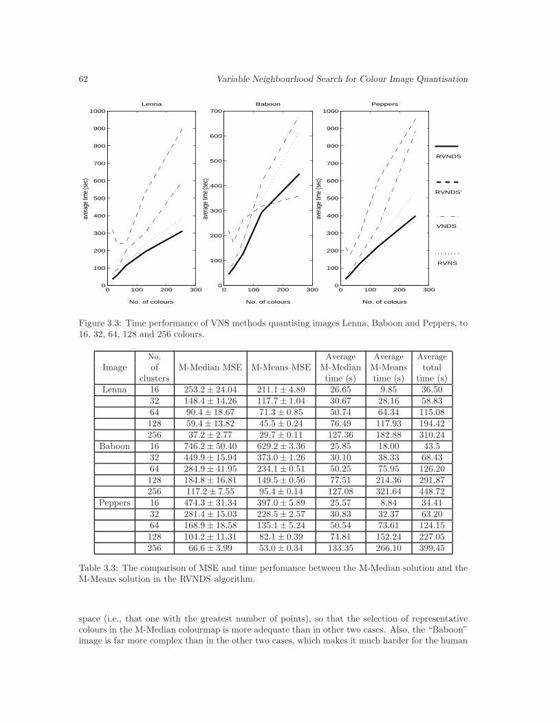
62 Variable Neighbourhood Search for Colour Image Quantisation
0 100 200 3000
100
200
300
400
500
600
700
800
900
1000
No. of colours
aver
age t
ime (
sec)
Lenna
0 100 200 3000
100
200
300
400
500
600
700
No. of colours
aver
age t
ime (
sec)
Baboon
0 100 200 3000
100
200
300
400
500
600
700
800
900
1000
No. of colours
aver
age t
ime (
sec)
Peppers
RVNDS
RVNDS’
VNDS
RVNS
Figure 3.3: Time performance of VNS methods quantising images Lenna, Baboon and Peppers, to16, 32, 64, 128 and 256 colours.
No. Average Average Average
Image of M-Median MSE M-Means MSE M-Median M-Means totalclusters time (s) time (s) time (s)
Lenna 16 253.2± 24.04 211.1± 4.89 26.65 9.85 36.5032 148.4± 14.26 117.7± 1.04 30.67 28.16 58.8364 90.4± 18.67 71.3± 0.85 50.74 64.34 115.08128 59.4± 13.82 45.5± 0.24 76.49 117.93 194.42256 37.2± 2.77 29.7± 0.11 127.36 182.88 310.24
Baboon 16 746.2± 50.40 629.2± 3.36 25.85 18.00 43.532 449.9± 15.94 373.0± 1.26 30.10 38.33 68.4364 284.9± 41.95 234.1± 0.51 50.25 75.95 126.20128 184.8± 16.81 149.5± 0.56 77.51 214.36 291.87256 117.2± 7.55 95.4± 0.14 127.08 321.64 448.72
Peppers 16 474.3± 31.34 397.0± 5.89 25.57 8.84 34.4132 281.4± 15.03 228.5± 2.57 30.83 32.37 63.2064 168.9± 18.58 135.1± 5.24 50.54 73.61 124.15128 104.2± 11.31 82.1± 0.39 74.81 152.24 227.05256 66.6± 3.99 53.0± 0.34 133.35 266.10 399.45
Table 3.3: The comparison of MSE and time perfomance between the M-Median solution and theM-Means solution in the RVNDS algorithm.
space (i.e., that one with the greatest number of points), so that the selection of representativecolours in the M-Median colourmap is more adequate than in other two cases. Also, the “Baboon”image is far more complex than in the other two cases, which makes it much harder for the human
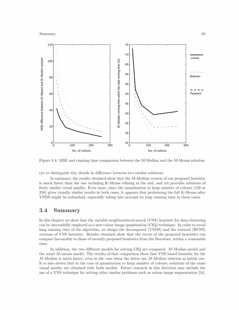
Summary 63
0 100 200 3000
20
40
60
80
100
120
No. of colours
0 100 200 30025
30
35
40
45
50
55
60
65
70
75
No. of colours
Lenna
Baboon
Peppers
MS
E d
iffer
ence
bet
wee
n M
−Mea
ns a
nd M
−Med
ian
solu
tion
M−M
edia
n ru
nnin
g tim
e w
ithin
the
tota
l run
ning
tim
e (%
)
Figure 3.4: MSE and running time comparison between the M-Median and the M-Means solution.
eye to distinguish tiny details in difference between two similar solutions.
In summary, the results obtained show that the M-Median version of our proposed heuristicis much faster than the one including K-Means refining in the end, and yet provides solutions offairly similar visual quality. Even more, since the quantisation to large number of colours (128 or256) gives visually similar results in both cases, it appears that performing the full K-Means afterVNDS might be redundant, especially taking into account its long running time in these cases.
3.4 Summary
In this chapter we show that the variable neighbourhood search (VNS) heuristic for data clusteringcan be successfully employed as a new colour image quantisation (CIQ) technique. In order to avoidlong running time of the algorithm, we design the decomposed (VNDS) and the reduced (RVNS)versions of VNS heuristic. Results obtained show that the errors of the proposed heuristics cancompare favourably to those of recently proposed heuristics from the literature, within a reasonabletime.
In addition, the two different models for solving CIQ are compared. M -Median model andthe usual M -means model. The results of that comparison show that VNS based heuristic for theM -Median is much faster, even in the case when the latter use M -Median solution as initial one.It is also shown that in the case of quantisation to large number of colours, solutions of the samevisual quality are obtained with both models. Future research in this direction may include theuse of a VNS technique for solving other similar problems such as colour image segmentation [54].

64 Variable Neighbourhood Search for Colour Image Quantisation
(a) (b)
Figure 3.5: “Lenna” quantised to 16 colours: (a) M-Median solution, (b) M-Means solution.
(a) (b)
Figure 3.6: “Lenna” quantised to 64 colours: (a) M-Median solution, (b) M-Means solution.
(a) (b)
Figure 3.7: “Lenna” quantised to 256 colours: (a) M-Median solution, (b) M-Means solution.

Summary 65
(a) (b)
Figure 3.8: “Baboon” quantised to 16 colours: (a) M-Median solution, (b) M-Means solution.
(a) (b)
Figure 3.9: “Baboon” quantised to 64 colours: (a) M-Median solution, (b) M-Means solution.
(a) (b)
Figure 3.10: “Baboon” quantised to 256 colours: (a) M-Median solution, (b) M-Means solution.
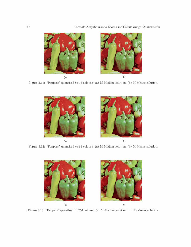
66 Variable Neighbourhood Search for Colour Image Quantisation
(a) (b)
Figure 3.11: “Peppers” quantised to 16 colours: (a) M-Median solution, (b) M-Means solution.
(a) (b)
Figure 3.12: “Peppers” quantised to 64 colours: (a) M-Median solution, (b) M-Means solution.
(a) (b)
Figure 3.13: “Peppers” quantised to 256 colours: (a) M-Median solution, (b) M-Means solution.

Chapter 4
Variable NeighbourhoodDecomposition Search for the 0-1MIP Problem
The concept of variable fixing in order to find solutions to MIP problems was conceived in the late1970s and early 1980s, when the first methods of this type for the pure 0-1 integer programmingproblems were proposed [21, 298]. This approach is sometimes referred to as a core approach,since the subproblems obtained by fixing a certain number of variables in a given MIP modelare sometimes called core problems. The terms hard variable fixing or diving are also present inthe literature [75]. The critical issue in this type of methods is the way in which the variablesto be fixed are chosen. Depending on the selection strategy and the way of manipulating theobtained subproblems, different MIP solution methods are obtained. Successful extensions ofthe basic method from [21] were proposed in [259, 269]. Another iterative scheme for the 0-1multidimensional knapsack problem, based on a dynamic fixation of the variables, was developed in[329]. This scheme also incorporates information about the search history, which is used to build upfeasible solutions and to select variables for a permanent/temporary fixation. In [234, 235], variableneighbourhood search was combined with a very large scale neighbourhood search to select variablesfor fixing (so called binding sets in the original papers [234, 235]) and conduct the investigationof subproblems, for the general assignment problem. This approach was further extended for0-1 mixed integer programming in general [233]. With the expansion of general-purpose MIPsolvers over the last decade, different hybridisations of MIP heuristics with commercial solversare becoming increasingly popular. A number of efficient heuristics, which perform some kindof variable fixing at each node of a B&B tree in the CPLEX MIP commercial solver, have beendeveloped so far. Relaxation induced neighbourhood search (RINS) [75] fixes the values of thevariables which are the same in the current continuous (i.e. LP) relaxation and in the incumbentintegral solution. Distance induced neighbourhood search [120] performs a more intelligent fixation,by taking into account the values of variables in the root LP relaxation and memorising occurrencesof different values during the search process, in addition to considering the values of the current LPrelaxation solution. Relaxation enforced neighbourhood search [32] is an extension of RINS, whichadditionally performs a large-scale neighbourhood search over the set of general integer variablesby an intelligent rebounding according to the current LP relaxation solution.
This chapter is organised as follows. In Section 4.1, a detailed description of the new VNDSheuristic for solving 0-1 MIP problems is described. Next, in Section 4.2, the performance of the
67

68 Variable Neighbourhood Decomposition Search for the 0-1 MIP Problem
VNDS method is analysed, compared to the other three state-of-the-art 0-1 MIP solution methodsand to the CPLEX MIP solver alone. Three methods used for comparison purposes are localbranching [104], variable neighbourhood branching [169] and relaxation induced neighbourhoodsearch [75]. They were described in detail in Chapter 2, Section 2.4. Last, in Section 4.3, somefinal remarks and conclusions are provided.
4.1 The VNDS-MIP Algorithm
In this section, a new variant of VNDS for solving 0-1 MIP problems, called VNDS-MIP, is pro-posed. This method combines a linear programming (LP) solver, MIP solver and VNS based MIPsolving method VND-MIP in order to efficiently solve a given 0-1 MIP problem. A systematichard variable fixing (or diving) is performed following the variable neighbourhood search rules.The variables to be fixed are chosen according to their distance from the corresponding linearrelaxation solution values. If there is an improvement, variable neighbourhood descent branchingis performed as the local search in the whole solution space.
The pseudo-code for VNDS-MIP is given in Figure 4.1. Input parameters for the VNDS-MIP algorithm are instance P of 0 − 1 MIP problem, parameter d, which defines the value ofvariable kstep, i.e., defines the number of variables to be released (set free) in each iteration of thealgorithm, the maximum running time allowed tmax, time tsub allowed for solving subproblems,time tvnd allowed for the VND-MIP procedure, time tmip allowed for call to the MIP solver withinthe VND-MIP procedure and maximum size rhsmax of a neighbourhood to be explored within theVND-MIP procedure.
At the beginning of the algorithm, the LP relaxation of the original problem P is solvedfirst, in order to obtain an optimal solution x (see line 1 in Figure 4.1). The value of the objectivefunction ctx provides a lower bound on the optimal value ν(P ) of P . Note that, if the optimalsolution x is integer feasible for P , the algorithm stops and returns x as an optimal solution for P .Then, an initial feasible solution x of the input problem P is generated (see line 2 in Figure 4.1).Although solving 0-1 MIP problems to feasibility alone is not always an easy task, we will hereassume that this step can be performed in a reasonable time. For more details on the 0-1 MIPfeasibility issues the reader is referred to Chapter 6. At each iteration of the VNDS-MIP proce-dure, the distances δj =| xj − xj | from the current incumbent solution values (xj)j∈B to theircorresponding LP relaxation solution values (xj)j∈B are computed and the variables xj , j ∈ B areindexed so that 0 ≤ δ1 ≤ δ2 ≤ . . . ≤ δp (where p =| B |). Then the subproblem P (x, {1, . . . , k}),obtained from the original problem P , is solved, where the first k variables are fixed to their valuesin the current incumbent solution x. If an improvement occurs, the VND-MIP procedure (see Fig-ure 4.2) is performed over the whole search space and the process is repeated. If not, the numberof fixed variables in the current subproblem is decreased. Note that by fixing only the variableswhose distance values are equal to zero, i.e., setting k = max{j ∈ B | δj = 0}, RINS scheme isobtained.
The specific implementation of the VND-MIP procedure used as a local search methodwithin the VNDS-MIP (see line 10 in Figure 4.1) is desribed next. Input parameters for the VND-MIP algorithm are instance P of the 0 − 1 MIP problem, total running time allowed tvnd, timetmip allowed for the MIP solver, maximum size rhsmax of the neighbourhood to be explored, andstarting solution x′. The output is new solution obtained. The VND-MIP pseudo-code is given inFigure 4.2.
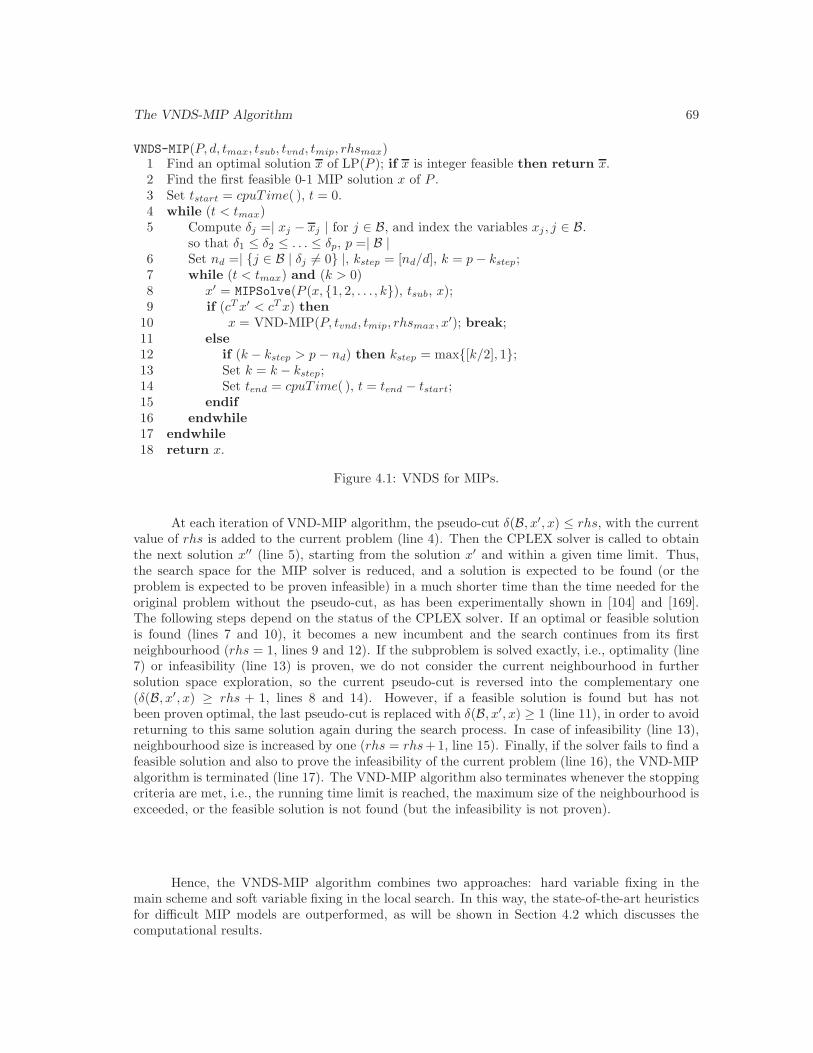
The VNDS-MIP Algorithm 69
VNDS-MIP(P, d, tmax, tsub, tvnd, tmip, rhsmax)1 Find an optimal solution x of LP(P ); if x is integer feasible then return x.2 Find the first feasible 0-1 MIP solution x of P .3 Set tstart = cpuT ime( ), t = 0.4 while (t < tmax)5 Compute δj =| xj − xj | for j ∈ B, and index the variables xj , j ∈ B.
so that δ1 ≤ δ2 ≤ . . . ≤ δp, p =| B |6 Set nd =| {j ∈ B | δj 6= 0} |, kstep = [nd/d], k = p− kstep;7 while (t < tmax) and (k > 0)8 x′ = MIPSolve(P (x, {1, 2, . . . , k}), tsub, x);9 if (cT x′ < cT x) then
10 x = VND-MIP(P, tvnd, tmip, rhsmax, x′); break;11 else12 if (k − kstep > p− nd) then kstep = max{[k/2], 1};13 Set k = k − kstep;14 Set tend = cpuT ime( ), t = tend − tstart;15 endif16 endwhile17 endwhile18 return x.
Figure 4.1: VNDS for MIPs.
At each iteration of VND-MIP algorithm, the pseudo-cut δ(B, x′, x) ≤ rhs, with the currentvalue of rhs is added to the current problem (line 4). Then the CPLEX solver is called to obtainthe next solution x′′ (line 5), starting from the solution x′ and within a given time limit. Thus,the search space for the MIP solver is reduced, and a solution is expected to be found (or theproblem is expected to be proven infeasible) in a much shorter time than the time needed for theoriginal problem without the pseudo-cut, as has been experimentally shown in [104] and [169].The following steps depend on the status of the CPLEX solver. If an optimal or feasible solutionis found (lines 7 and 10), it becomes a new incumbent and the search continues from its firstneighbourhood (rhs = 1, lines 9 and 12). If the subproblem is solved exactly, i.e., optimality (line7) or infeasibility (line 13) is proven, we do not consider the current neighbourhood in furthersolution space exploration, so the current pseudo-cut is reversed into the complementary one(δ(B, x′, x) ≥ rhs + 1, lines 8 and 14). However, if a feasible solution is found but has notbeen proven optimal, the last pseudo-cut is replaced with δ(B, x′, x) ≥ 1 (line 11), in order to avoidreturning to this same solution again during the search process. In case of infeasibility (line 13),neighbourhood size is increased by one (rhs = rhs+1, line 15). Finally, if the solver fails to find afeasible solution and also to prove the infeasibility of the current problem (line 16), the VND-MIPalgorithm is terminated (line 17). The VND-MIP algorithm also terminates whenever the stoppingcriteria are met, i.e., the running time limit is reached, the maximum size of the neighbourhood isexceeded, or the feasible solution is not found (but the infeasibility is not proven).
Hence, the VNDS-MIP algorithm combines two approaches: hard variable fixing in themain scheme and soft variable fixing in the local search. In this way, the state-of-the-art heuristicsfor difficult MIP models are outperformed, as will be shown in Section 4.2 which discusses thecomputational results.
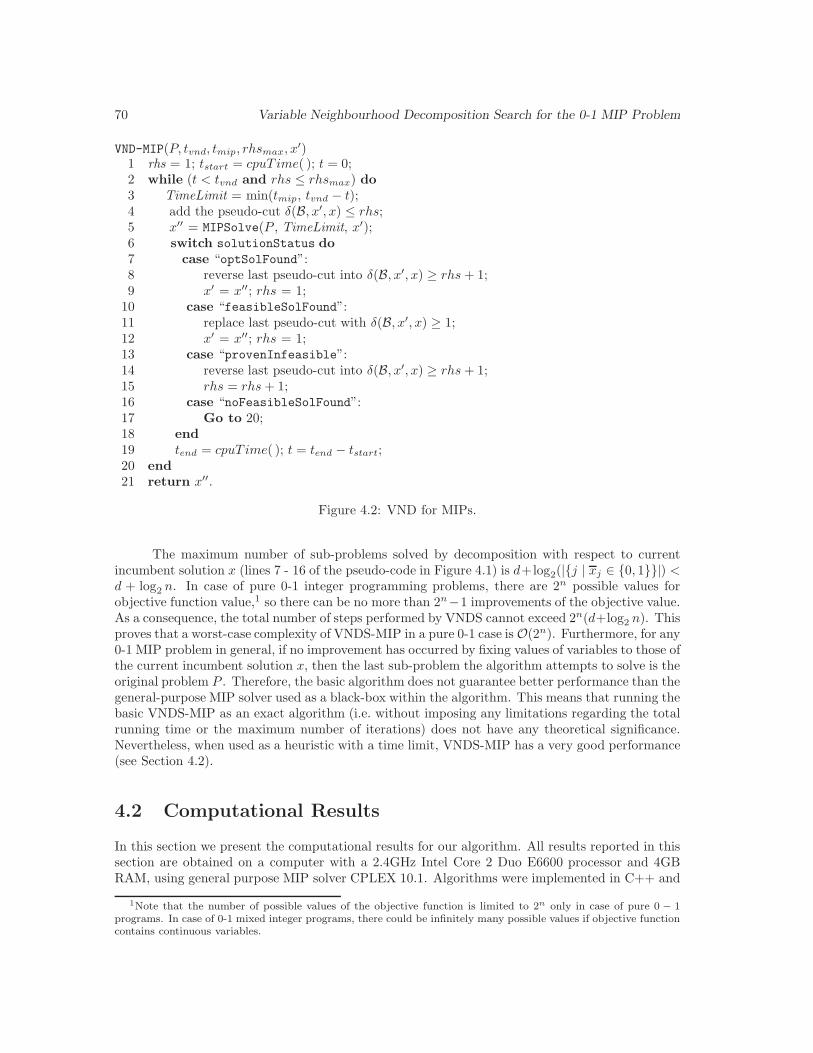
70 Variable Neighbourhood Decomposition Search for the 0-1 MIP Problem
VND-MIP(P, tvnd, tmip, rhsmax, x′)1 rhs = 1; tstart = cpuT ime( ); t = 0;2 while (t < tvnd and rhs ≤ rhsmax) do3 TimeLimit = min(tmip, tvnd − t);4 add the pseudo-cut δ(B, x′, x) ≤ rhs;5 x′′ = MIPSolve(P , TimeLimit, x′);6 switch solutionStatus do7 case “optSolFound”:8 reverse last pseudo-cut into δ(B, x′, x) ≥ rhs + 1;9 x′ = x′′; rhs = 1;
10 case “feasibleSolFound”:11 replace last pseudo-cut with δ(B, x′, x) ≥ 1;12 x′ = x′′; rhs = 1;13 case “provenInfeasible”:14 reverse last pseudo-cut into δ(B, x′, x) ≥ rhs + 1;15 rhs = rhs + 1;16 case “noFeasibleSolFound”:17 Go to 20;18 end19 tend = cpuT ime( ); t = tend − tstart;20 end21 return x′′.
Figure 4.2: VND for MIPs.
The maximum number of sub-problems solved by decomposition with respect to currentincumbent solution x (lines 7 - 16 of the pseudo-code in Figure 4.1) is d+log2(|{j | xj ∈ {0, 1}}|) <d + log2 n. In case of pure 0-1 integer programming problems, there are 2n possible values forobjective function value,1 so there can be no more than 2n−1 improvements of the objective value.As a consequence, the total number of steps performed by VNDS cannot exceed 2n(d+log2 n). Thisproves that a worst-case complexity of VNDS-MIP in a pure 0-1 case is O(2n). Furthermore, for any0-1 MIP problem in general, if no improvement has occurred by fixing values of variables to those ofthe current incumbent solution x, then the last sub-problem the algorithm attempts to solve is theoriginal problem P . Therefore, the basic algorithm does not guarantee better performance than thegeneral-purpose MIP solver used as a black-box within the algorithm. This means that running thebasic VNDS-MIP as an exact algorithm (i.e. without imposing any limitations regarding the totalrunning time or the maximum number of iterations) does not have any theoretical significance.Nevertheless, when used as a heuristic with a time limit, VNDS-MIP has a very good performance(see Section 4.2).
4.2 Computational Results
In this section we present the computational results for our algorithm. All results reported in thissection are obtained on a computer with a 2.4GHz Intel Core 2 Duo E6600 processor and 4GBRAM, using general purpose MIP solver CPLEX 10.1. Algorithms were implemented in C++ and
1Note that the number of possible values of the objective function is limited to 2n only in case of pure 0 − 1programs. In case of 0-1 mixed integer programs, there could be infinitely many possible values if objective functioncontains continuous variables.

Computational Results 71
compiled within Microsoft Visual Studio 2005.
Methods compared. The VNDS-MIP is compared with the four other recent MIP solutionmethods: variable neighbourhood branching (VNB) [169], local branching (LB) [104], relaxationinduced neighbourhood search (RINS) [75] and the CPLEX MIP solver (with all default optionsbut without RINS heuristic). The VNB and the LB use CPLEX MIP solver as a black box. TheRINS heuristic is directly incorporated within a CPLEX branch-and-cut tree search algorithm.It should be noted that the objective function values for LB, VNB and RINS reported here aresometimes different from those given in the original papers. The reasons for this are the use of adifferent version of CPLEX and the use of a different computer.
Test bed. The 29 test instances which are considered here for comparison purposes are the sameas those previously used for testing performances of LB and VNB (see [104], [169]) and most ofthe instances used for testing RINS (see [75]). The characteristics of this test bed are given inTable 4.1: the number of constraints is given in column one, the total number of variables is givenin column two, column three indicates the number of binary variables, and column four indicatesthe best known published objective value so far.
In order to clearly show the differences between all the techniques, the models are dividedinto four groups, according to the gap between the best and the worst solution obtained usingthe five methods. Problems are defined as very small-spread, small-spread, medium-spread, andlarge-spread if the gap mentioned is less than 1%, between 1% and 10%, between 10% and 100%and larger than 100%, respectively. A similar way of grouping the test instances was first presentedin Danna et al. [75], where the problems were divided into three sets. We use this way of groupingthe problems mainly for the graphical representation of our results.
CPLEX parameters. As mentioned earlier, the CPLEX MIP solver is used in each methodcompared. A more detailed explanation of the way in which its parameters are used is providedhere. For LB, VNB and VNDS, the CPX PARAM MIP EMPHASIS is set to FEASIBILITY for the firstfeasible solution, and then changed to the default BALANCED option after the first feasible solutionhas been found. Furthermore, for all instances except for van, all heuristics for finding the first fea-sible solution are turned off, i.e., both parameters CPX PARAM HEUR FREQ and CPX PARAM RINS HEUR
are set to −1. This is done because of the empirical observation that the use of heuristic withinCPLEX slows down the search process, without improving the quality of the final solution.
After the first feasible solution has been found, the local heuristics frequency (parameterCPX PARAM HEUR FREQ) is set to 100. For the instance van, the first feasible solution cannot befound in this way within the given time limit, due to its numerical instability. So, for this instance,both parameters CPX PARAM HEUR FREQ and CPX PARAM RINS HEUR are set to 100 in order to obtainthe first feasible solution, and after this the RINS heuristic is turned off.
Termination. All methods were run for 5 hours (tmax = 18, 000 seconds), the same length oftime as in the papers about local branching ([104]) and VNB ([169]). An exception is the NSR8K,which is the largest instance in the test bed. Due to the long time required for the first feasiblesolution to be attained (more than 13,000 seconds), 15 hours are allowed for solving this problem(tmax = 54, 000).
VNDS Implementation. In order to evaluate the performance of the algorithm and its sen-sitivity to the parameter values, different parameter settings were tried out. As the goal was tomake the algorithm user-friendly, an effort has been made to reduce the number of parameters. Inaddition, it was aimed to use the same values of parameters for testing most of the test instances.As the result of preliminary testing, the two variants of VNDS for MIP were obtained, which differ
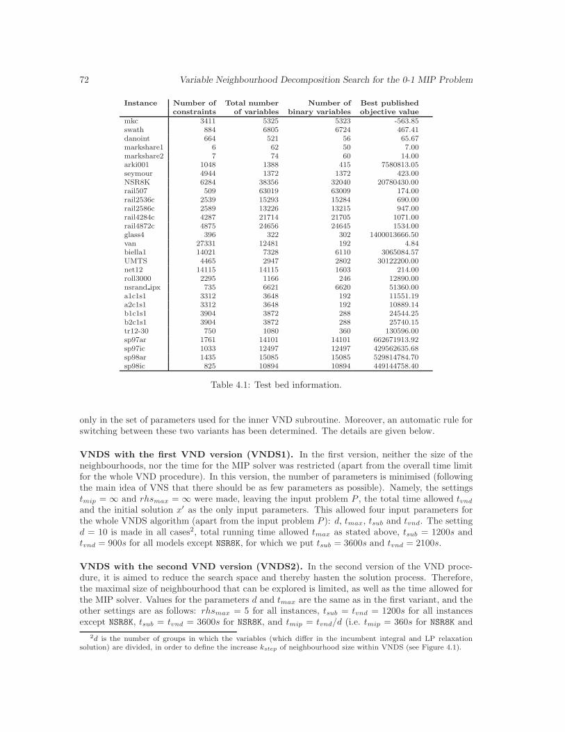
72 Variable Neighbourhood Decomposition Search for the 0-1 MIP Problem
Instance Number of Total number Number of Best published
constraints of variables binary variables objective value
mkc 3411 5325 5323 -563.85swath 884 6805 6724 467.41danoint 664 521 56 65.67markshare1 6 62 50 7.00markshare2 7 74 60 14.00arki001 1048 1388 415 7580813.05seymour 4944 1372 1372 423.00NSR8K 6284 38356 32040 20780430.00rail507 509 63019 63009 174.00rail2536c 2539 15293 15284 690.00rail2586c 2589 13226 13215 947.00rail4284c 4287 21714 21705 1071.00rail4872c 4875 24656 24645 1534.00glass4 396 322 302 1400013666.50van 27331 12481 192 4.84biella1 14021 7328 6110 3065084.57UMTS 4465 2947 2802 30122200.00net12 14115 14115 1603 214.00roll3000 2295 1166 246 12890.00nsrand ipx 735 6621 6620 51360.00a1c1s1 3312 3648 192 11551.19a2c1s1 3312 3648 192 10889.14b1c1s1 3904 3872 288 24544.25b2c1s1 3904 3872 288 25740.15tr12-30 750 1080 360 130596.00sp97ar 1761 14101 14101 662671913.92sp97ic 1033 12497 12497 429562635.68sp98ar 1435 15085 15085 529814784.70sp98ic 825 10894 10894 449144758.40
Table 4.1: Test bed information.
only in the set of parameters used for the inner VND subroutine. Moreover, an automatic rule forswitching between these two variants has been determined. The details are given below.
VNDS with the first VND version (VNDS1). In the first version, neither the size of theneighbourhoods, nor the time for the MIP solver was restricted (apart from the overall time limitfor the whole VND procedure). In this version, the number of parameters is minimised (followingthe main idea of VNS that there should be as few parameters as possible). Namely, the settingstmip = ∞ and rhsmax = ∞ were made, leaving the input problem P , the total time allowed tvnd
and the initial solution x′ as the only input parameters. This allowed four input parameters forthe whole VNDS algorithm (apart from the input problem P ): d, tmax, tsub and tvnd. The settingd = 10 is made in all cases2, total running time allowed tmax as stated above, tsub = 1200s andtvnd = 900s for all models except NSR8K, for which we put tsub = 3600s and tvnd = 2100s.
VNDS with the second VND version (VNDS2). In the second version of the VND proce-dure, it is aimed to reduce the search space and thereby hasten the solution process. Therefore,the maximal size of neighbourhood that can be explored is limited, as well as the time allowed forthe MIP solver. Values for the parameters d and tmax are the same as in the first variant, and theother settings are as follows: rhsmax = 5 for all instances, tsub = tvnd = 1200s for all instancesexcept NSR8K, tsub = tvnd = 3600s for NSR8K, and tmip = tvnd/d (i.e. tmip = 360s for NSR8K and
2d is the number of groups in which the variables (which differ in the incumbent integral and LP relaxation
solution) are divided, in order to define the increase kstep of neighbourhood size within VNDS (see Figure 4.1).
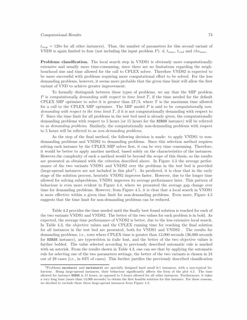
Computational Results 73
tmip = 120s for all other instances). Thus, the number of parameters for this second variant ofVNDS is again limited to four (not including the input problem P ): d, tmax, tvnd and rhsmax.
Problems classification. The local search step in VNDS1 is obviously more computationallyextensive and usually more time-consuming, since there are no limitations regarding the neigh-bourhood size and time allowed for the call to CPLEX solver. Therefore VNDS2 is expected tobe more successful with problems requiring more computational effort to be solved. For the lessdemanding problems, however, it seems more probable that the given time limit will allow the firstvariant of VND to achieve greater improvement.
To formally distinguish between these types of problems, we say that the MIP problemP is computationally demanding with respect to time limit T , if the time needed for the defaultCPLEX MIP optimiser to solve it is greater than 2T/3, where T is the maximum time allowedfor a call to the CPLEX MIP optimiser. The MIP model P is said to be computationally non-demanding with respect to the time limit T , if it is not computationally demanding with respect toT . Since the time limit for all problems in the test bed used is already given, the computationallydemanding problems with respect to 5 hours (or 15 hours for the NSR8K instance) will be referredto as demanding problems. Similarly, the computationally non-demanding problems with respectto 5 hours will be referred to as non-demanding problems.
As the step of the final method, the following decision is made: to apply VNDS1 to non-demanding problems and VNDS2 to demanding problems. Since this selection method requiressolving each instance by the CPLEX MIP solver first, it can be very time consuming. Therefore,it would be better to apply another method, based solely on the characteristics of the instances.However,the complexity of such a method would be beyond the scope of this thesis, so the resultsare presented as obtained with the criterion described above. In Figure 4.3 the average perfor-mance of the two variants VNDS1 and VNDS2 over the problems in the test bed is provided(large-spread instances are not included in this plot3). As predicted, it is clear that in the earlystage of the solution process, heuristic VNDS2 improves faster. However, due to the longer timeallowed for solving subproblems, VNDS1 improves its average performance later. This pattern ofbehaviour is even more evident in Figure 4.4, where we presented the average gap change overtime for demanding problems. However, from Figure 4.5, it is clear that a local search in VNDS1is more effective within a given time limit for non-demanding problems. Even more, Figure 4.5suggests that the time limit for non-demanding problems can be reduced.
Table 4.2 provides the time needed until the finally best found solution is reached for each ofthe two variants VNDS1 and VNDS2. The better of the two values for each problem is in bold. Asexpected, the average time performance of VNDS2 is better, due to the less extensive local search.In Table 4.3, the objective values and the CPLEX running time for reaching the final solutionfor all instances in the test bed are presented, both for VNDS1 and VNDS2 . The results fordemanding problems, i.e., rows where CPLEX time is greater than 12,000 seconds (36,000 secondsfor NSR8K instance), are typewritten in italic font, and the better of the two objective values isfurther bolded. The value selected according to previously described automatic rule is markedwith an asterisk. From the results shown in Table 4.3, one can see that by applying the automaticrule for selecting one of the two parameters settings, the better of the two variants is chosen in 24out of 29 cases (i.e., in 83% of cases). This further justifies the previously described classification
3Problems marshare1 and markshare2 are specially designed hard small 0-1 instances, with a non-typical be-haviour. Being large-spread instances, their behaviour significantly affects the form of the plot 4.3. The timeallowed for instance NSR8K is 15 hours, as opposed to 5 hours allowed for all other instances. Furthermore, it takesa very long time (more than 13,000 seconds) to obtain the first feasible solution for this instance. For these reasons,we decided to exclude these three large-spread instances from Figure 4.3.
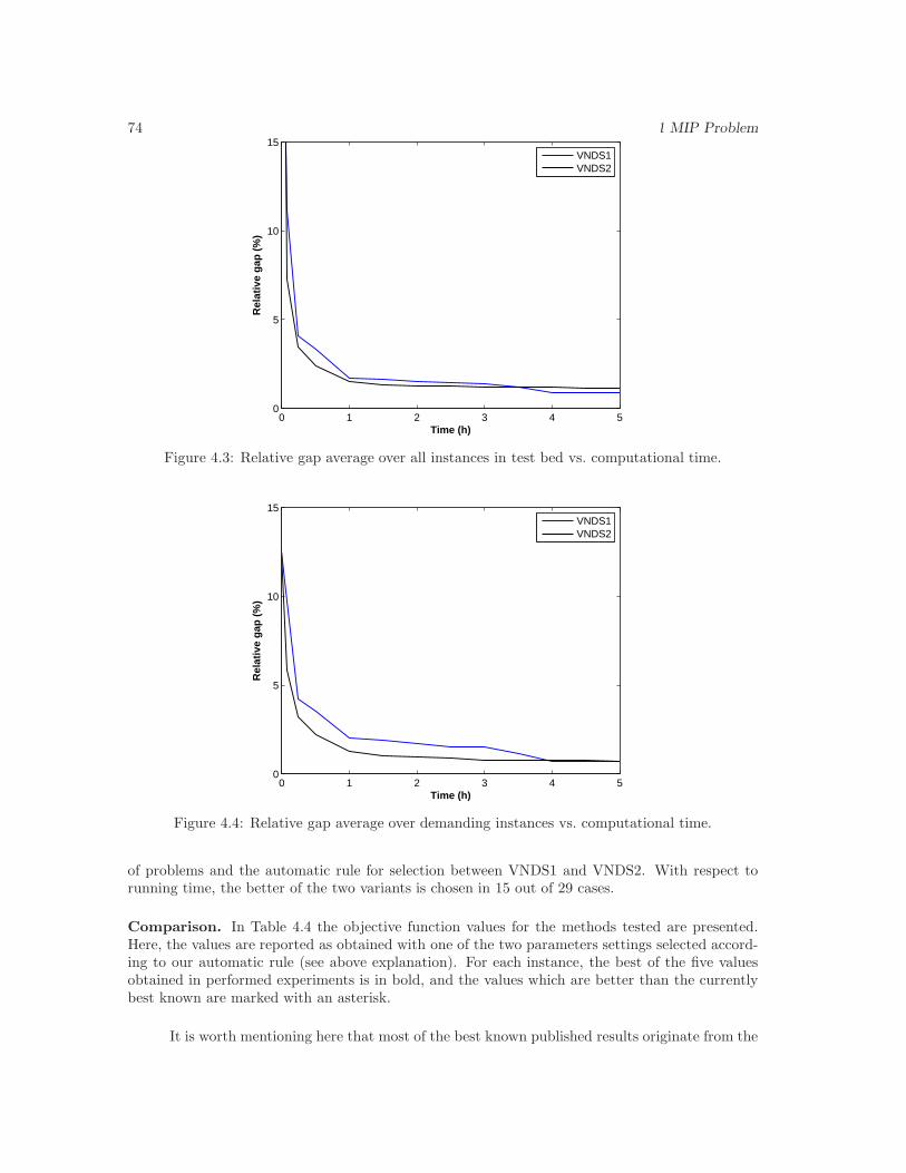
74 Variable Neighbourhood Decomposition Search for the 0-1 MIP Problem
0 1 2 3 4 50
5
10
15
Time (h)
Rel
ativ
e g
ap (
%)
VNDS1VNDS2
Figure 4.3: Relative gap average over all instances in test bed vs. computational time.
0 1 2 3 4 50
5
10
15
Time (h)
Rel
ativ
e g
ap (
%)
VNDS1VNDS2
Figure 4.4: Relative gap average over demanding instances vs. computational time.
of problems and the automatic rule for selection between VNDS1 and VNDS2. With respect torunning time, the better of the two variants is chosen in 15 out of 29 cases.
Comparison. In Table 4.4 the objective function values for the methods tested are presented.Here, the values are reported as obtained with one of the two parameters settings selected accord-ing to our automatic rule (see above explanation). For each instance, the best of the five valuesobtained in performed experiments is in bold, and the values which are better than the currentlybest known are marked with an asterisk.
It is worth mentioning here that most of the best known published results originate from the
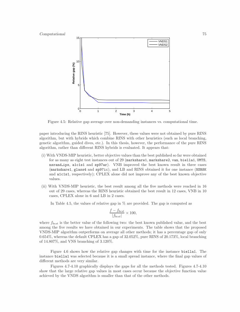
Computational Results 75
0 1 2 3 4 50
5
10
15
Time (h)
Rel
ativ
e g
ap (
%)
VNDS1VNDS2
Figure 4.5: Relative gap average over non-demanding instances vs. computational time.
paper introducing the RINS heuristic [75]. However, these values were not obtained by pure RINSalgorithm, but with hybrids which combine RINS with other heuristics (such as local branching,genetic algorithm, guided dives, etc.). In this thesis, however, the performance of the pure RINSalgorithm, rather than different RINS hybrids is evaluated. It appears that:
(i) With VNDS-MIP heuristic, better objective values than the best published so far were obtainedfor as many as eight test instances out of 29 (markshare1, markshare2, van, biella1, UMTS,nsrand ipx, a1c1s1 and sp97ar). VNB improved the best known result in three cases(markshare1, glass4 and sp97ic), and LB and RINS obtained it for one instance (NSR8Kand a1c1s1, respectively); CPLEX alone did not improve any of the best known objectivevalues.
(ii) With VNDS-MIP heuristic, the best result among all the five methods were reached in 16out of 29 cases, whereas the RINS heuristic obtained the best result in 12 cases, VNB in 10cases, CPLEX alone in 6 and LB in 2 cases.
In Table 4.5, the values of relative gap in % are provided. The gap is computed as
f − fbest
|fbest|× 100,
where fbest is the better value of the following two: the best known published value, and the bestamong the five results we have obtained in our experiments. The table shows that the proposedVNDS-MIP algorithm outperforms on average all other methods; it has a percentage gap of only0.654%, whereas the default CPLEX has a gap of 32.052%, pure RINS of 20.173%, local branchingof 14.807%, and VNS branching of 3.120%.
Figure 4.6 shows how the relative gap changes with time for the instance biella1. Theinstance biella1 was selected because it is a small spread instance, where the final gap values ofdifferent methods are very similar.
Figures 4.7-4.10 graphically displays the gaps for all the methods tested. Figures 4.7-4.10show that the large relative gap values in most cases occur because the objective function valueachieved by the VNDS algorithm is smaller than that of the other methods.
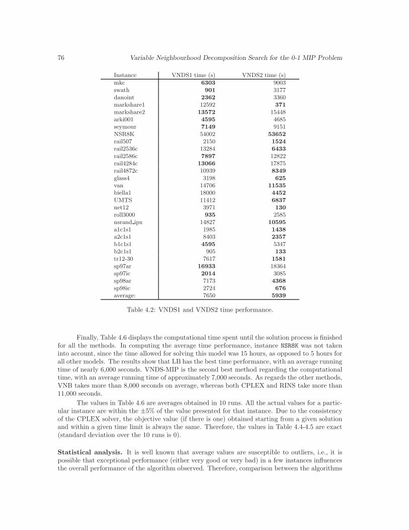
76 Variable Neighbourhood Decomposition Search for the 0-1 MIP Problem
Instance VNDS1 time (s) VNDS2 time (s)
mkc 6303 9003swath 901 3177danoint 2362 3360markshare1 12592 371
markshare2 13572 15448arki001 4595 4685seymour 7149 9151NSR8K 54002 53652
rail507 2150 1524
rail2536c 13284 6433
rail2586c 7897 12822rail4284c 13066 17875rail4872c 10939 8349
glass4 3198 625
van 14706 11535
biella1 18000 4452
UMTS 11412 6837
net12 3971 130
roll3000 935 2585nsrand ipx 14827 10595
a1c1s1 1985 1438
a2c1s1 8403 2357
b1c1s1 4595 5347b2c1s1 905 133
tr12-30 7617 1581
sp97ar 16933 18364sp97ic 2014 3085sp98ar 7173 4368
sp98ic 2724 676
average: 7650 5939
Table 4.2: VNDS1 and VNDS2 time performance.
Finally, Table 4.6 displays the computational time spent until the solution process is finishedfor all the methods. In computing the average time performance, instance NSR8K was not takeninto account, since the time allowed for solving this model was 15 hours, as opposed to 5 hours forall other models. The results show that LB has the best time performance, with an average runningtime of nearly 6,000 seconds. VNDS-MIP is the second best method regarding the computationaltime, with an average running time of approximately 7,000 seconds. As regards the other methods,VNB takes more than 8,000 seconds on average, whereas both CPLEX and RINS take more than11,000 seconds.
The values in Table 4.6 are averages obtained in 10 runs. All the actual values for a partic-ular instance are within the ±5% of the value presented for that instance. Due to the consistencyof the CPLEX solver, the objective value (if there is one) obtained starting from a given solutionand within a given time limit is always the same. Therefore, the values in Table 4.4-4.5 are exact(standard deviation over the 10 runs is 0).
Statistical analysis. It is well known that average values are susceptible to outliers, i.e., it ispossible that exceptional performance (either very good or very bad) in a few instances influencesthe overall performance of the algorithm observed. Therefore, comparison between the algorithms
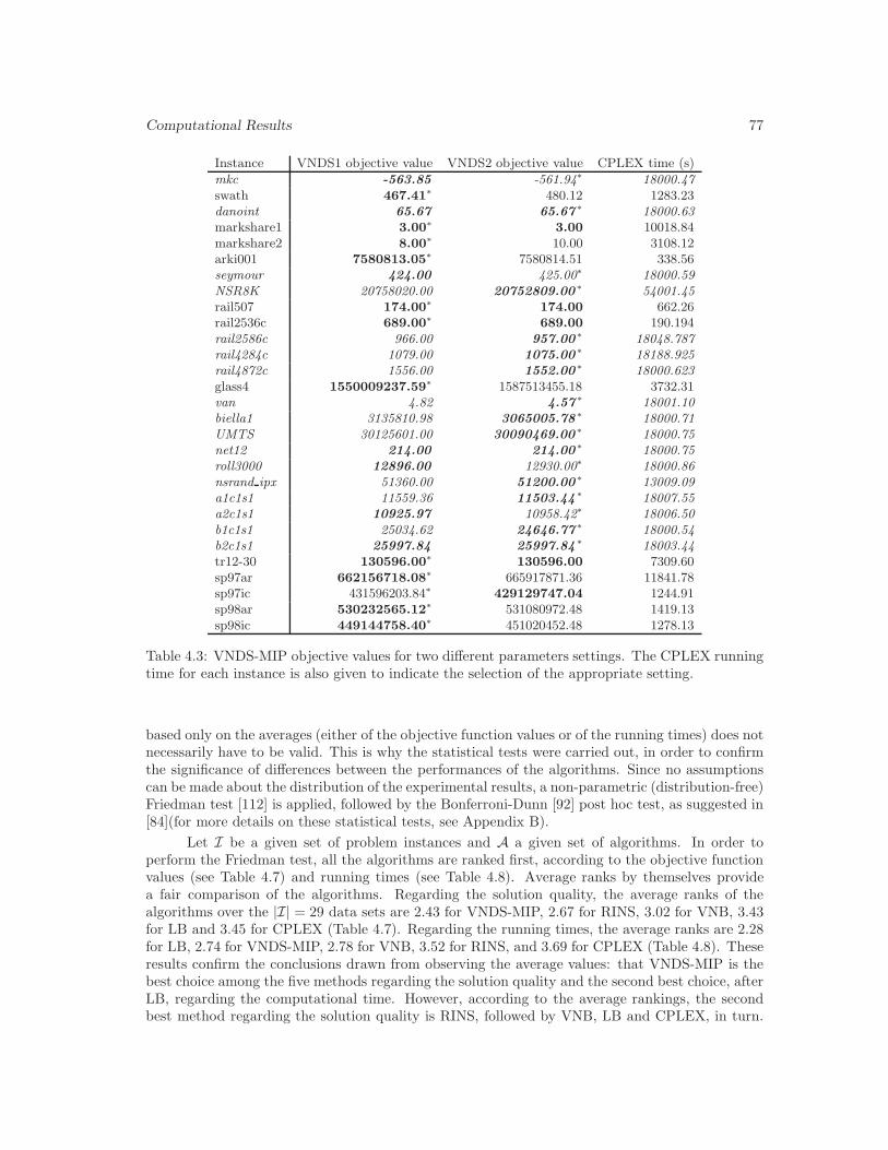
Computational Results 77
Instance VNDS1 objective value VNDS2 objective value CPLEX time (s)
mkc -563.85 -561.94∗ 18000.47
swath 467.41∗ 480.12 1283.23
danoint 65.67 65.67 ∗ 18000.63
markshare1 3.00∗
3.00 10018.84markshare2 8.00
∗ 10.00 3108.12arki001 7580813.05
∗ 7580814.51 338.56seymour 424.00 425.00∗ 18000.59
NSR8K 20758020.00 20752809.00 ∗ 54001.45
rail507 174.00∗
174.00 662.26rail2536c 689.00
∗
689.00 190.194rail2586c 966.00 957.00 ∗ 18048.787
rail4284c 1079.00 1075.00 ∗ 18188.925
rail4872c 1556.00 1552.00 ∗ 18000.623
glass4 1550009237.59∗ 1587513455.18 3732.31
van 4.82 4.57 ∗ 18001.10
biella1 3135810.98 3065005.78 ∗ 18000.71
UMTS 30125601.00 30090469.00 ∗ 18000.75
net12 214.00 214.00 ∗ 18000.75
roll3000 12896.00 12930.00∗ 18000.86
nsrand ipx 51360.00 51200.00 ∗ 13009.09
a1c1s1 11559.36 11503.44 ∗ 18007.55
a2c1s1 10925.97 10958.42∗ 18006.50
b1c1s1 25034.62 24646.77 ∗ 18000.54
b2c1s1 25997.84 25997.84 ∗ 18003.44
tr12-30 130596.00∗
130596.00 7309.60sp97ar 662156718.08
∗ 665917871.36 11841.78sp97ic 431596203.84∗
429129747.04 1244.91sp98ar 530232565.12
∗ 531080972.48 1419.13sp98ic 449144758.40
∗ 451020452.48 1278.13
Table 4.3: VNDS-MIP objective values for two different parameters settings. The CPLEX runningtime for each instance is also given to indicate the selection of the appropriate setting.
based only on the averages (either of the objective function values or of the running times) does notnecessarily have to be valid. This is why the statistical tests were carried out, in order to confirmthe significance of differences between the performances of the algorithms. Since no assumptionscan be made about the distribution of the experimental results, a non-parametric (distribution-free)Friedman test [112] is applied, followed by the Bonferroni-Dunn [92] post hoc test, as suggested in[84](for more details on these statistical tests, see Appendix B).
Let I be a given set of problem instances and A a given set of algorithms. In order toperform the Friedman test, all the algorithms are ranked first, according to the objective functionvalues (see Table 4.7) and running times (see Table 4.8). Average ranks by themselves providea fair comparison of the algorithms. Regarding the solution quality, the average ranks of thealgorithms over the |I| = 29 data sets are 2.43 for VNDS-MIP, 2.67 for RINS, 3.02 for VNB, 3.43for LB and 3.45 for CPLEX (Table 4.7). Regarding the running times, the average ranks are 2.28for LB, 2.74 for VNDS-MIP, 2.78 for VNB, 3.52 for RINS, and 3.69 for CPLEX (Table 4.8). Theseresults confirm the conclusions drawn from observing the average values: that VNDS-MIP is thebest choice among the five methods regarding the solution quality and the second best choice, afterLB, regarding the computational time. However, according to the average rankings, the secondbest method regarding the solution quality is RINS, followed by VNB, LB and CPLEX, in turn.
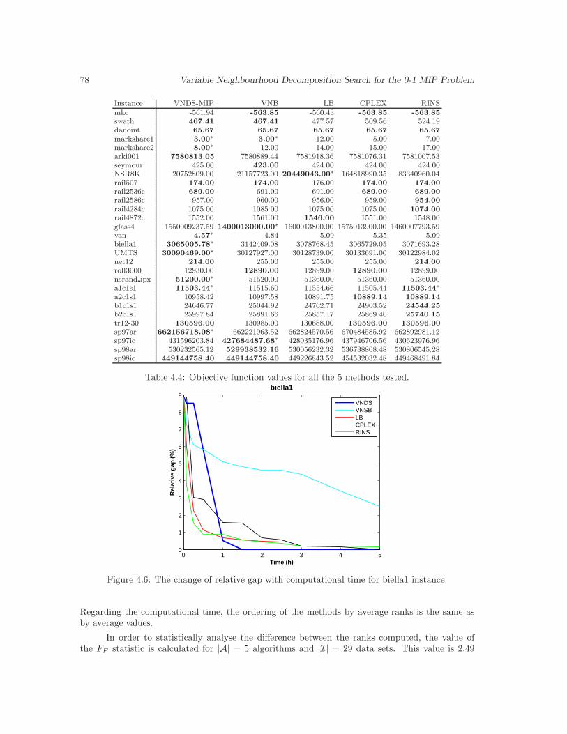
78 Variable Neighbourhood Decomposition Search for the 0-1 MIP Problem
Instance VNDS-MIP VNB LB CPLEX RINSmkc -561.94 -563.85 -560.43 -563.85 -563.85
swath 467.41 467.41 477.57 509.56 524.19danoint 65.67 65.67 65.67 65.67 65.67
markshare1 3.00∗ 3.00∗ 12.00 5.00 7.00markshare2 8.00∗ 12.00 14.00 15.00 17.00arki001 7580813.05 7580889.44 7581918.36 7581076.31 7581007.53seymour 425.00 423.00 424.00 424.00 424.00NSR8K 20752809.00 21157723.00 20449043.00∗ 164818990.35 83340960.04rail507 174.00 174.00 176.00 174.00 174.00
rail2536c 689.00 691.00 691.00 689.00 689.00
rail2586c 957.00 960.00 956.00 959.00 954.00
rail4284c 1075.00 1085.00 1075.00 1075.00 1074.00
rail4872c 1552.00 1561.00 1546.00 1551.00 1548.00glass4 1550009237.59 1400013000.00∗ 1600013800.00 1575013900.00 1460007793.59van 4.57∗ 4.84 5.09 5.35 5.09biella1 3065005.78∗ 3142409.08 3078768.45 3065729.05 3071693.28UMTS 30090469.00∗ 30127927.00 30128739.00 30133691.00 30122984.02net12 214.00 255.00 255.00 255.00 214.00
roll3000 12930.00 12890.00 12899.00 12890.00 12899.00nsrand ipx 51200.00∗ 51520.00 51360.00 51360.00 51360.00a1c1s1 11503.44∗ 11515.60 11554.66 11505.44 11503.44∗
a2c1s1 10958.42 10997.58 10891.75 10889.14 10889.14
b1c1s1 24646.77 25044.92 24762.71 24903.52 24544.25
b2c1s1 25997.84 25891.66 25857.17 25869.40 25740.15
tr12-30 130596.00 130985.00 130688.00 130596.00 130596.00
sp97ar 662156718.08∗ 662221963.52 662824570.56 670484585.92 662892981.12sp97ic 431596203.84 427684487.68∗ 428035176.96 437946706.56 430623976.96sp98ar 530232565.12 529938532.16 530056232.32 536738808.48 530806545.28sp98ic 449144758.40 449144758.40 449226843.52 454532032.48 449468491.84
Table 4.4: Objective function values for all the 5 methods tested.
0 1 2 3 4 50
1
2
3
4
5
6
7
8
9biella1
Time (h)
Rel
ativ
e g
ap (
%)
VNDSVNSBLBCPLEXRINS
Figure 4.6: The change of relative gap with computational time for biella1 instance.
Regarding the computational time, the ordering of the methods by average ranks is the same asby average values.
In order to statistically analyse the difference between the ranks computed, the value ofthe FF statistic is calculated for |A| = 5 algorithms and |I| = 29 data sets. This value is 2.49
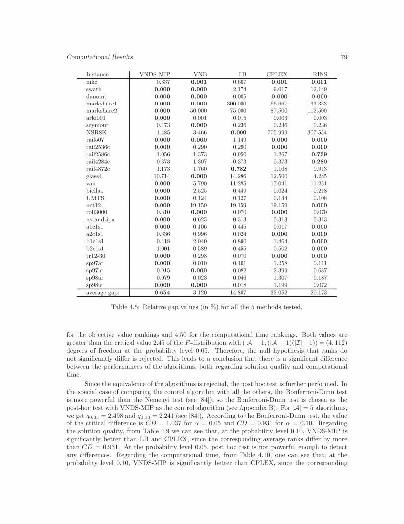
Computational Results 79
Instance VNDS-MIP VNB LB CPLEX RINS
mkc 0.337 0.001 0.607 0.001 0.001
swath 0.000 0.000 2.174 9.017 12.149danoint 0.000 0.000 0.005 0.000 0.000
markshare1 0.000 0.000 300.000 66.667 133.333markshare2 0.000 50.000 75.000 87.500 112.500arki001 0.000 0.001 0.015 0.003 0.003seymour 0.473 0.000 0.236 0.236 0.236NSR8K 1.485 3.466 0.000 705.999 307.554rail507 0.000 0.000 1.149 0.000 0.000
rail2536c 0.000 0.290 0.290 0.000 0.000
rail2586c 1.056 1.373 0.950 1.267 0.739
rail4284c 0.373 1.307 0.373 0.373 0.280
rail4872c 1.173 1.760 0.782 1.108 0.913glass4 10.714 0.000 14.286 12.500 4.285van 0.000 5.790 11.285 17.041 11.251biella1 0.000 2.525 0.449 0.024 0.218UMTS 0.000 0.124 0.127 0.144 0.108net12 0.000 19.159 19.159 19.159 0.000
roll3000 0.310 0.000 0.070 0.000 0.070nsrand ipx 0.000 0.625 0.313 0.313 0.313a1c1s1 0.000 0.106 0.445 0.017 0.000
a2c1s1 0.636 0.996 0.024 0.000 0.000
b1c1s1 0.418 2.040 0.890 1.464 0.000
b2c1s1 1.001 0.589 0.455 0.502 0.000
tr12-30 0.000 0.298 0.070 0.000 0.000
sp97ar 0.000 0.010 0.101 1.258 0.111sp97ic 0.915 0.000 0.082 2.399 0.687sp98ar 0.079 0.023 0.046 1.307 0.187sp98ic 0.000 0.000 0.018 1.199 0.072
average gap: 0.654 3.120 14.807 32.052 20.173
Table 4.5: Relative gap values (in %) for all the 5 methods tested.
for the objective value rankings and 4.50 for the computational time rankings. Both values aregreater than the critical value 2.45 of the F -distribution with (|A|−1, (|A|−1)(|I|−1)) = (4, 112)degrees of freedom at the probability level 0.05. Therefore, the null hypothesis that ranks donot significantly differ is rejected. This leads to a conclusion that there is a significant differencebetween the performances of the algorithms, both regarding solution quality and computationaltime.
Since the equivalence of the algorithms is rejected, the post hoc test is further performed. Inthe special case of comparing the control algorithm with all the others, the Bonferroni-Dunn testis more powerful than the Nemenyi test (see [84]), so the Bonferroni-Dunn test is chosen as thepost-hoc test with VNDS-MIP as the control algorithm (see Appendix B). For |A| = 5 algorithms,we get q0.05 = 2.498 and q0.10 = 2.241 (see [84]). According to the Bonferroni-Dunn test, the valueof the critical difference is CD = 1.037 for α = 0.05 and CD = 0.931 for α = 0.10. Regardingthe solution quality, from Table 4.9 we can see that, at the probability level 0.10, VNDS-MIP issignificantly better than LB and CPLEX, since the corresponding average ranks differ by morethan CD = 0.931. At the probability level 0.05, post hoc test is not powerful enough to detectany differences. Regarding the computational time, from Table 4.10, one can see that, at theprobability level 0.10, VNDS-MIP is significantly better than CPLEX, since the corresponding
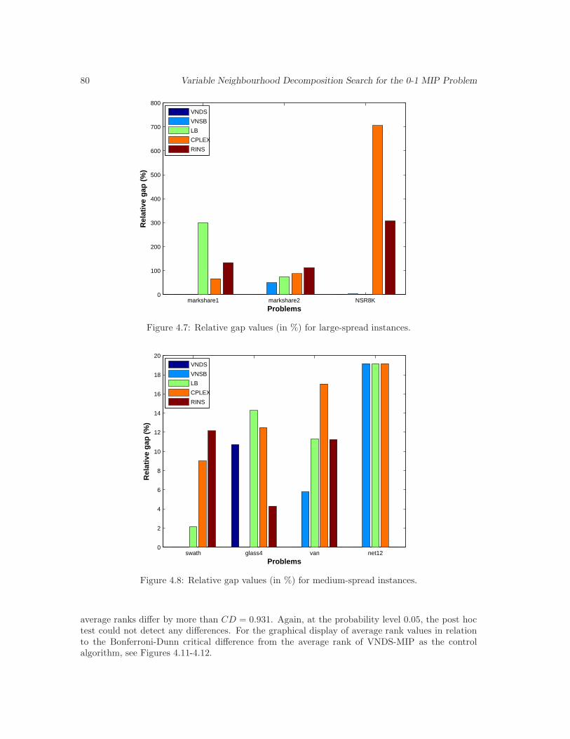
80 Variable Neighbourhood Decomposition Search for the 0-1 MIP Problem
markshare1 markshare2 NSR8K0
100
200
300
400
500
600
700
800
Problems
Rel
ativ
e g
ap (
%)
VNDS
VNSB
LB
CPLEX
RINS
Figure 4.7: Relative gap values (in %) for large-spread instances.
swath glass4 van net120
2
4
6
8
10
12
14
16
18
20
Problems
Rel
ativ
e g
ap (
%)
VNDS
VNSB
LB
CPLEX
RINS
Figure 4.8: Relative gap values (in %) for medium-spread instances.
average ranks differ by more than CD = 0.931. Again, at the probability level 0.05, the post hoctest could not detect any differences. For the graphical display of average rank values in relationto the Bonferroni-Dunn critical difference from the average rank of VNDS-MIP as the controlalgorithm, see Figures 4.11-4.12.
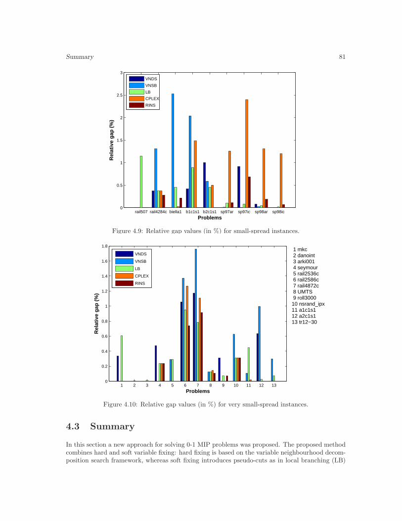
Summary 81
rail507 rail4284c biella1 b1c1s1 b2c1s1 sp97ar sp97ic sp98ar sp98ic0
0.5
1
1.5
2
2.5
3
Problems
Rel
ativ
e g
ap (
%)
VNDS
VNSB
LB
CPLEX
RINS
Figure 4.9: Relative gap values (in %) for small-spread instances.
1 2 3 4 5 6 7 8 9 10 11 12 130
0.2
0.4
0.6
0.8
1
1.2
1.4
1.6
1.8
Problems
Rel
ativ
e g
ap (
%)
VNDS
VNSB
LB
CPLEX
RINS
1 mkc 2 danoint 3 arki001 4 seymour 5 rail2536c 6 rail2586c 7 rail4872c 8 UMTS 9 roll300010 nsrand_ipx11 a1c1s112 a2c1s113 tr12−30
Figure 4.10: Relative gap values (in %) for very small-spread instances.
4.3 Summary
In this section a new approach for solving 0-1 MIP problems was proposed. The proposed methodcombines hard and soft variable fixing: hard fixing is based on the variable neighbourhood decom-position search framework, whereas soft fixing introduces pseudo-cuts as in local branching (LB)
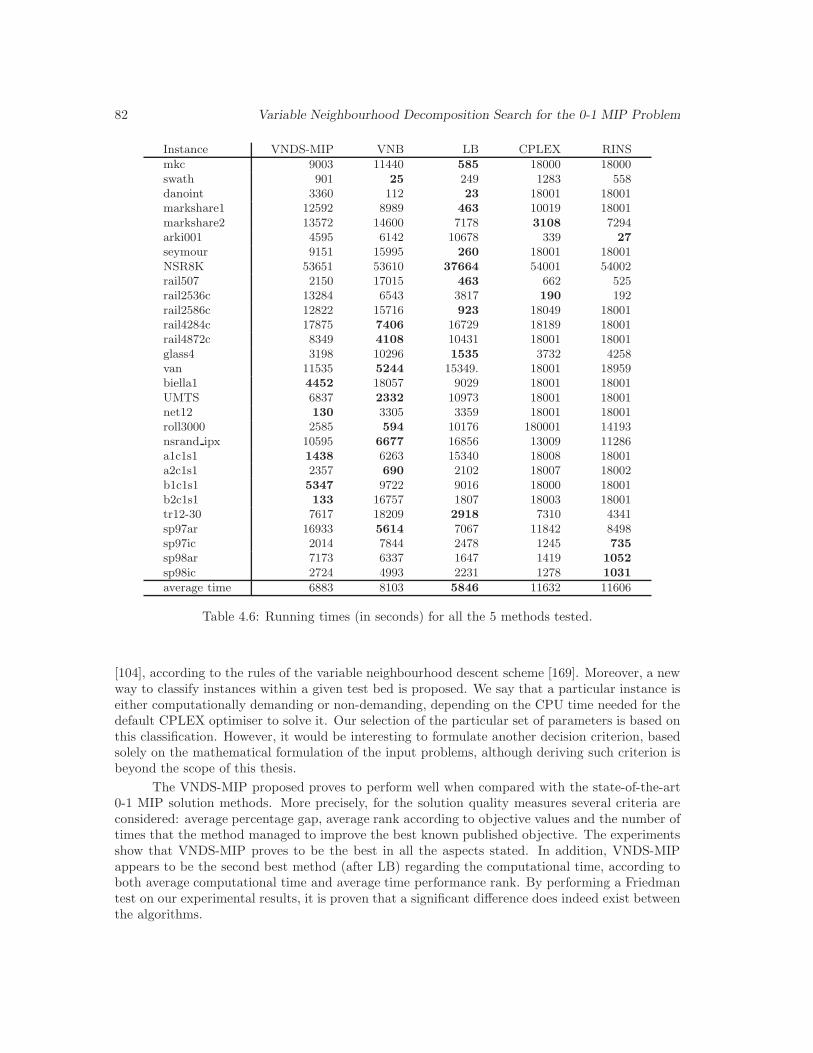
82 Variable Neighbourhood Decomposition Search for the 0-1 MIP Problem
Instance VNDS-MIP VNB LB CPLEX RINS
mkc 9003 11440 585 18000 18000swath 901 25 249 1283 558danoint 3360 112 23 18001 18001markshare1 12592 8989 463 10019 18001markshare2 13572 14600 7178 3108 7294arki001 4595 6142 10678 339 27
seymour 9151 15995 260 18001 18001NSR8K 53651 53610 37664 54001 54002rail507 2150 17015 463 662 525rail2536c 13284 6543 3817 190 192rail2586c 12822 15716 923 18049 18001rail4284c 17875 7406 16729 18189 18001rail4872c 8349 4108 10431 18001 18001glass4 3198 10296 1535 3732 4258van 11535 5244 15349. 18001 18959biella1 4452 18057 9029 18001 18001UMTS 6837 2332 10973 18001 18001net12 130 3305 3359 18001 18001roll3000 2585 594 10176 180001 14193nsrand ipx 10595 6677 16856 13009 11286a1c1s1 1438 6263 15340 18008 18001a2c1s1 2357 690 2102 18007 18002b1c1s1 5347 9722 9016 18000 18001b2c1s1 133 16757 1807 18003 18001tr12-30 7617 18209 2918 7310 4341sp97ar 16933 5614 7067 11842 8498sp97ic 2014 7844 2478 1245 735
sp98ar 7173 6337 1647 1419 1052
sp98ic 2724 4993 2231 1278 1031
average time 6883 8103 5846 11632 11606
Table 4.6: Running times (in seconds) for all the 5 methods tested.
[104], according to the rules of the variable neighbourhood descent scheme [169]. Moreover, a newway to classify instances within a given test bed is proposed. We say that a particular instance iseither computationally demanding or non-demanding, depending on the CPU time needed for thedefault CPLEX optimiser to solve it. Our selection of the particular set of parameters is based onthis classification. However, it would be interesting to formulate another decision criterion, basedsolely on the mathematical formulation of the input problems, although deriving such criterion isbeyond the scope of this thesis.
The VNDS-MIP proposed proves to perform well when compared with the state-of-the-art0-1 MIP solution methods. More precisely, for the solution quality measures several criteria areconsidered: average percentage gap, average rank according to objective values and the number oftimes that the method managed to improve the best known published objective. The experimentsshow that VNDS-MIP proves to be the best in all the aspects stated. In addition, VNDS-MIPappears to be the second best method (after LB) regarding the computational time, according toboth average computational time and average time performance rank. By performing a Friedmantest on our experimental results, it is proven that a significant difference does indeed exist betweenthe algorithms.

Summary 83
Instance VNDS-MIP VNB LB CPLEX RINS
mkc 4.00 2.00 5.00 2.00 2.00swath 1.50 1.50 3.00 4.00 5.00danoint 2.50 2.50 5.00 2.50 2.50markshare1 1.50 1.50 5.00 3.00 4.00markshare2 1.00 2.00 3.00 4.00 5.00arki001 1.00 2.00 5.00 4.00 3.00seymour 5.00 1.00 3.00 3.00 3.00NSR8K 2.00 3.00 1.00 5.00 4.00rail507 2.50 2.50 5.00 2.50 2.50rail2536c 2.00 4.50 4.50 2.00 2.00rail2586c 3.00 5.00 2.00 4.00 1.00rail4284c 3.00 5.00 3.00 3.00 1.00rail4872c 4.00 5.00 1.00 3.00 2.00glass4 3.00 1.00 5.00 4.00 2.00van 1.00 2.00 3.50 5.00 3.50biella1 1.00 5.00 4.00 2.00 3.00UMTS 1.00 3.00 4.00 5.00 2.00net12 1.50 4.00 4.00 4.00 1.50roll3000 5.00 1.50 3.50 1.50 3.50nsrand ipx 1.00 5.00 3.00 3.00 3.00a1c1s1 1.50 4.00 5.00 3.00 1.50a2c1s1 4.00 5.00 3.00 1.50 1.50b1c1s1 2.00 5.00 3.00 4.00 1.00b2c1s1 5.00 4.00 2.00 3.00 1.00tr12-30 2.00 5.00 4.00 2.00 2.00sp97ar 1.00 2.00 3.00 5.00 4.00sp97ic 4.00 1.00 2.00 5.00 3.00sp98ar 3.00 1.00 2.00 5.00 4.00sp98ic 1.50 1.50 3.00 5.00 4.00
average ranks 2.43 3.02 3.43 3.45 2.67
Table 4.7: Algorithm rankings by the objective function values for all instances.

84 Variable Neighbourhood Decomposition Search for the 0-1 MIP Problem
Instance VNDS-MIP VNB LB CPLEX RINS
mkc 2.00 3.00 1.00 4.50 4.50swath 4.00 1.00 2.00 5.00 3.00danoint 3.00 2.00 1.00 4.50 4.50markshare1 4.00 2.00 1.00 3.00 5.00markshare2 4.00 5.00 2.00 1.00 3.00arki001 3.00 4.00 5.00 2.00 1.00seymour 2.00 3.00 1.00 4.50 4.50NSR8K 2.50 2.50 1.00 4.50 4.50rail507 4.00 5.00 1.00 3.00 2.00rail2536c 5.00 4.00 3.00 1.50 1.50rail2586c 3.00 2.00 1.00 4.50 4.50rail4284c 3.00 1.00 2.00 4.00 5.00rail4872c 2.00 1.00 3.00 4.50 4.50glass4 2.00 5.00 1.00 3.00 4.00van 2.00 1.00 3.00 4.00 5.00biella1 1.00 5.00 2.00 3.50 3.50UMTS 2.00 1.00 3.00 4.50 4.50net12 1.00 2.00 3.00 4.50 4.50roll3000 2.00 1.00 3.00 5.00 4.00nsrand ipx 2.00 1.00 5.00 4.00 3.00a1c1s1 1.00 2.00 3.00 4.50 4.50a2c1s1 3.00 1.00 2.00 4.50 4.50b1c1s1 1.00 3.00 2.00 4.50 4.50b2c1s1 1.00 3.00 2.00 4.50 4.50tr12-30 3.00 5.00 1.00 4.00 2.00sp97ar 5.00 1.00 2.00 4.00 3.00sp97ic 3.00 5.00 4.00 2.00 1.00sp98ar 5.00 4.00 3.00 2.00 1.00sp98ic 4.00 5.00 3.00 2.00 1.00
average ranks 2.74 2.78 2.28 3.69 3.52
Table 4.8: Algorithm rankings by the running time values for all instances.
ALGORITHM (average rank) VNB (3.02) LB (3.43) CPLEX (3.45) RINS (2.67)
Difference from VNDS-MIP rank (2.43) 0.59 1.00 1.02 0.24
Table 4.9: Objective value average rank differences from the average rank of the control algorithmVNDS-MIP.
ALGORITHM (average rank) VNB (2.78) LB (2.28) CPLEX (3.69) RINS (3.52)
Difference from VNDS-MIP rank (2.74) 0.03 -0.47 0.95 0.78
Table 4.10: Running time average rank differences from the average rank of the control algorithmVNDS-MIP.
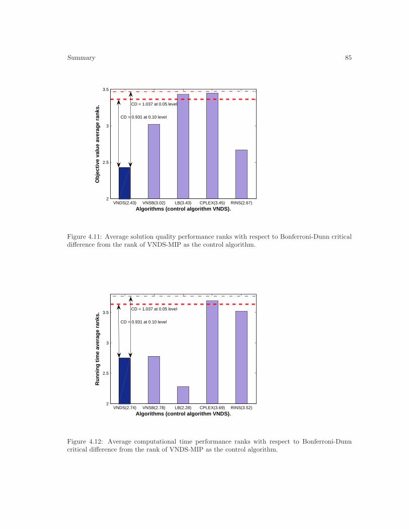
Summary 85
VNDS(2.43) VNSB(3.02) LB(3.43) CPLEX(3.45) RINS(2.67)2
2.5
3
3.5
Algorithms (control algorithm VNDS).
Ob
ject
ive
valu
e av
erag
e ra
nks
.
CD = 0.931 at 0.10 level
CD = 1.037 at 0.05 level
Figure 4.11: Average solution quality performance ranks with respect to Bonferroni-Dunn criticaldifference from the rank of VNDS-MIP as the control algorithm.
VNDS(2.74) VNSB(2.78) LB(2.28) CPLEX(3.69) RINS(3.52)2
2.5
3
3.5
Algorithms (control algorithm VNDS).
Ru
nn
ing
tim
e av
erag
e ra
nks
.
CD = 0.931 at 0.10 level
CD = 1.037 at 0.05 level
Figure 4.12: Average computational time performance ranks with respect to Bonferroni-Dunncritical difference from the rank of VNDS-MIP as the control algorithm.

86 Variable Neighbourhood Decomposition Search for the 0-1 MIP Problem
Chapter 5
Applications of VNDS to SomeSpecific 0-1 MIP Problems
In Chapter 4, it has be shown that the proposed VNDS-MIP heuristic can be very effective insolving 0-1 MIP problems in general. In this chapter, attempts are made to further enhance thebasic variant of VNDS-MIP and test the resulting heuristics on a few specific 0-1 MIP problems.The problems considered are the multidimensional knapsack problem in Section 5.1, the barge con-tainer ship routing problem in Section 5.2 and the two-stage stochastic mixed integer programmingproblem in Section 5.3.
5.1 The Multidimensional Knapsack Problem
In this section, new matheuristics for solving the multidimensional knapsack problem (MKP) areproposed. They are based on various decomposition strategies incorporated within the variableneighbourhood search, including both one-level and two-level decomposition. Basically, they canbe viewed as enhancements of the basic VNDS-MIP scheme proposed in Chapter 4. In all pro-posed heuristics, pseudo-cuts are used in order to reduce the search space and to diversify thesearch process. Beside being competitive with the current state-of-the-art heuristics for MKP,this approach has led to 63 best known lower bound values and to 3 new lower bound values ontwo representative sets of MKP instances (for a total of 108 instances), studied for a long time.In addition, it is proven that two of the proposed methods converge to an optimal solution if nolimitations regarding the execution time or the number of iterations are imposed.
The multidimensional knapsack problem (MKP) is a resource allocation problem which canbe formulated as follows:
(5.1) (MKP)
maxn∑
j=1
cjxj
subject ton∑
j=1
aijxj ≤ bi ∀i ∈M = {1, 2, . . . , m}
xj ∈ {0, 1} ∀j ∈ N = {1, 2, . . . , n}
Here, n is the number of items and m is the number of knapsack constraints. The right handside bi (i ∈M) represents the capacity of knapsack i. The matrix A = [aij ] is the weights matrix,whose element aij represents the resource consumption of the item j ∈ N in the knapsack i ∈M .
87
88 Applications of VNDS to Some Specific 0-1 MIP Problems
The profit income for the item j ∈ N is denoted by cj (j ∈ N). Being a special case of the 0-1mixed integer programming problem (1.6), MKP is often used as a benchmark model for testinggeneral purpose combinatorial optimisation methods.
A wide range of practical problems in business, engineering and science, can be modeled asMKP problems. They include the capital budgeting problem, cargo loading, allocating processorsin a huge distributed computer system, cutting stock problem, delivery of groceries in vehicleswith multiple compartments and many more. Since MKP is known to be np-hard [115], therewere numerous contributions over several decades to the development of both exact (mainly forthe case m = 1, see, for instance, [222, 258, 261], and for m > 1, see, for instance [41, 111, 116])and heuristic (for example [42, 58, 147, 326]) solution methods for MKP. For a complete review ofthese developments and applications of MKP, the reader is referred to [109, 328].
The mathematical programming formulation of MKP is especially convenient for the appli-cation of some general purpose solver. However, due to the complexity of the problem, sometimesit is not possible to obtain an optimal solution in this way. This is why a huge variety of prob-lem specific heuristics has been tailored, their drawback being that they cannot be applied toa general class of problems. An approach for generating and exploiting small sub-problems wassuggested in [121], based on the selection of consistent variables, depending on how frequentlythey attain particular values in good solutions and on how much disruption they would cause tothese solutions if changed. More recently, a variety of neighbourhood search heuristics for solvingoptimisation problems have emerged, such as variable neighbourhood search (VNS) proposed in[237], large neighbourhood search (LNS) introduced in [294] and the large-scale neighbourhoodsearch in [10]. In 2005, Glover proposed an adaptive memory projection (AMP) method for pureand mixed integer programming [124], which combines the principle of projection techniques withthe adaptive memory processes of tabu search to set some explicit or implicit variables to someparticular values. This philosophy gives a useful basis for unifying and extending a number of otherprocedures: LNS, local branching (LB) proposed in [104], the relaxation induced neighbourhoodsearch (RINS) proposed in [75], variable neighbourhood branching (VNB) [169], or the global tabusearch intensification using dynamic programming (TS-DP) [327] among others. LNS and RINShave been applied successfully to solve large-scale mixed integer programming problems. TS-DPis a hybrid method, combining adaptive memory and sparse dynamic programming to explore thesearch space, in which a move evaluation involves solving a reduced problem through dynamic pro-gramming at each iteration. Following the ideas of LB and RINS, another method for solving 0-1MIP problems was proposed in [207](see also Chapter 4). It is based on the principles of variableneighbourhood decomposition search (VNDS) [168]. This method uses the solution of the linearprogramming relaxation of the initial problem to define sub-problems to be solved within the VNDSframework. In [298], a convergent algorithm for pure 0-1 integer programming was proposed. Itsolves a series of small sub-problems generated by exploiting information obtained through a seriesof relaxations. In further text, we refer to this basic algorithm as the linear programming-basedalgorithm (LPA). Hanafi and Wilbaut have proposed several enhanced versions of the Soyster’sexact algorithm (see [154, 326]), by using a so called MIP relaxation of the problem. The firstheuristic, which employs only the MIP relaxation, is referred to as the iterative relaxation basedheuristic (IRH). The second one, in which MIP and LP relaxations are used in a parallel way, isreferred to as the iterative independent relaxation based heuristic (IIRH).
This section is organised as follows. Subsection 5.1.1, provides an overview of the existingLPA, IRH and IIRH heuristics for MKP. In Subsection 5.1.2, the new heuristics are presented,based on the mixed integer and linear programming relaxations of the problem and the VNDSprinciple. Next, in Subsection 5.1.4, computational results are presented and discussed in an effortto assess and analyse the performance of the proposed algorithms. In Subsection 5.1.5, someoutlines and conclusions are provided.
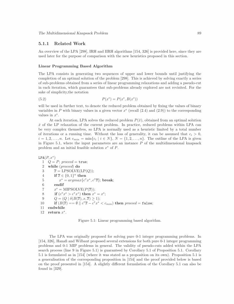
The Multidimensional Knapsack Problem 89
5.1.1 Related Work
An overview of the LPA [298], IRH and IIRH algorithms [154, 326] is provided here, since they areused later for the purpose of comparison with the new heuristics proposed in this section.
Linear Programming Based Algorithm
The LPA consists in generating two sequences of upper and lower bounds until justifying thecompletion of an optimal solution of the problem [298]. This is achieved by solving exactly a seriesof sub-problems obtained from a series of linear programming relaxations and adding a pseudo-cutin each iteration, which guarantees that sub-problems already explored are not revisited. For thesake of simplicity,the notation
(5.2) P (x0) = P (x0, B(x0))
will be used in further text, to denote the reduced problem obtained by fixing the values of binaryvariables in P with binary values in a given vector x0 (recall (2.4) and (2.9)) to the correspondingvalues in x0.
At each iteration, LPA solves the reduced problem P (x), obtained from an optimal solutionx of the LP relaxation of the current problem. In practice, reduced problems within LPA canbe very complex themselves, so LPA is normally used as a heuristic limited by a total numberof iterations or a running time. Without the loss of generality, it can be assumed that ci > 0,i = 1, 2, . . . , n. Let cmin = min{ci | i ∈ N}, N = {1, 2, . . . , n}. The outline of the LPA is givenin Figure 5.1, where the input parameters are an instance P of the multidimensional knapsackproblem and an initial feasible solution x∗ of P .
LPA(P, x∗)1 Q = P ; proceed = true;2 while (proceed) do3 x = LPSOLVE(LP(Q));4 if x ∈ {0, 1}n then5 x∗ = argmax{ctx∗, ctx}; break;6 endif7 x0 = MIPSOLVE(P (x));8 if (ctx0 > ctx∗) then x∗ = x0;9 Q = (Q | δ(B(x), x, x) ≥ 1);
10 if (B(x) == ∅ || ctx− ctx∗ < cmin) then proceed = false;11 endwhile12 return x∗.
Figure 5.1: Linear programming based algorithm.
The LPA was originally proposed for solving pure 0-1 integer programming problems. In[154, 326], Hanafi and Wilbaut proposed several extensions for both pure 0-1 integer programmingproblems and 0-1 MIP problems in general. The validity of pseudo-cuts added within the LPAsearch process (line 9 in Figure 5.1) is guaranteed by Corollary 5.1 of Proposition 5.1. Corollary5.1 is formulated as in [154] (where it was stated as a proposition on its own). Proposition 5.1 isa generalisation of the corresponding proposition in [154] and the proof provided below is basedon the proof presented in [154]. A slightly different formulation of the Corollary 5.1 can also befound in [329].

90 Applications of VNDS to Some Specific 0-1 MIP Problems
Proposition 5.1 Let P be a given 0− 1 mixed integer programming problem as defined in (1.6),
x0 ∈ {0, 1}|B| × Z+0
|G|× R+
0
|C|and J ⊆ B. An optimal solution of P is either an optimal solution
of the reduced problem P (x0, J), or an optimal solution of the problem (P | δ(J, x0, x) ≥ 1).
Proof. It is obvious that
ν(P ) = min{ν((P | δ(J, x0, x) = 0)), ν((P | δ(J, x0, x) ≥ 1))}
(recall that ν(P ) denotes the optimal value of P ). Since P (x0, J) = (P | δ(J, x0, x) = 0), if anoptimal solution of P is not optimal for P (x0, J), it has to be optimal for (P | δ(J, x0, x) ≥ 1). �
Corollary 5.1 Let P be a given 0− 1 mixed integer programming problem, x a solution of LP(P )and x0 an optimal solution of the reduced problem P (x). An optimal solution of P is either thesolution x0 or an optimal solution of the problem (P | δ(B(x), x, x) ≥ 1).
Proof. Corollary 5.1 is obtained from Proposition 5.1 by substituting x0 = x and J = B(x). �Proposition 5.1 and Corollary 5.1 are formulated and proved for minimisation problems. Analogousresults also hold for the case of maximisation. Therefore, the results of Proposition 5.1 andCorollary 5.1 (in their maximisation counterparts) are valid for the multidimensional knapsackproblem. Corollary 5.1 implies Theorem 5.1, which states the finite convergence of the LPA[154, 325]. The proof of Theorem 5.1 is similar as in [325].
Theorem 5.1 The LPA converges to an optimal solution of the input problem or indicates thatthe problem is infeasible in a finite number of iterations.
Proof. There are(nk
)2k possible LP solution vectors x with exactly k integer components. Hence,
there are∑n
k=0
(nk
)2k =
∑nk=0
(nk
)2k1n−k = 3n possible LP solution vectors x having integer
components. However, if x is integer feasible, the algorithm stops. Therefore, the number ofvectors whose all components are integer should be subtracted from the previously calculated totalnumber of LP solutions to obtain the maximum number of LPA iterations. Thus, the total numberof LPA iterations is limited by 3n − 2n.
Let F (Q) denote the feasible set of an optimisation problem Q. Let further P k denote theproblem considered in the kth iteration of LPA, P k+1 the problem obtained from P k by addingthe pseudo-cut in line 9 in Figure 5.1 to P k and xk the solution of LP(P k). If
F k =
k⋃
i=1
F (P (xi, B(xi))),
then F (P ) = F k ∪ F (P k) and F k ∩ F (P k) = ∅. The incumbent best solution after k iterations ofLPA is x∗k, such that
cx∗k = max{cx | x ∈ F k}.
According to Corollary 5.1, ν(P ) = max{cx∗k, max{cx | x ∈ F (P k)}}. Since LPA finishes in afinite number of iterations ktot, in the last iteration of LPA we have:
ν(P ) = max{cx∗ktot , max{cx | x ∈ F (P ktot)}}.
If P ktot is infeasible, i.e. F (P ktot) = ∅, then x∗ktot is an optimal solution of P . Otherwise, ν(P ) =max{cx∗ktot , ν(P ktot)} and LPA returns either cx∗ktot or an optimal solution of P ktot , whicheveris better. �
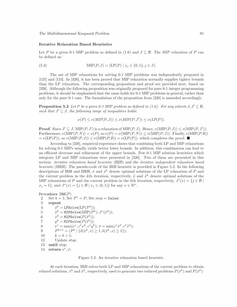
The Multidimensional Knapsack Problem 91
Iterative Relaxation Based Heuristics
Let P be a given 0-1 MIP problem as defined in (1.6) and J ⊆ B. The MIP relaxation of P canbe defined as:
(5.3) MIP(P, J) = (LP(P ) | xj ∈ {0, 1}, j ∈ J).
The use of MIP relaxations for solving 0-1 MIP problems was independently proposed in[125] and [153]. In [326], it has been proved that MIP relaxation normally supplies tighter boundsthan the LP relaxation. The corresponding proposition and proof are provided next, based on[326]. Although the following proposition was originally proposed for pure 0-1 integer programmingproblems, it should be emphasised that the same holds for 0-1 MIP problems in general, rather thanonly for the pure 0-1 case. The formulation of the proposition from [326] is amended accordingly.
Proposition 5.2 Let P be a given 0-1 MIP problem as defined in (1.6). For any subsets J, J ′ ⊆ B,such that J ′ ⊆ J , the following range of inequalities holds:
ν(P ) ≤ ν(MIP(P, J)) ≤ ν(MIP(P, J ′)) ≤ ν(LP(P )).
Proof. Since J ′ ⊆ J , MIP(P, J ′) is a relaxation of MIP(P, J). Hence, ν(MIP(P, J)) ≤ ν(MIP(P, J ′)).Furthermore, ν(MIP(P, N)) = ν(P ), so ν(P ) = ν(MIP(P, N)) ≤ ν(MIP(P, J)). Finally, ν(MIP(P, ∅))= ν(LP(P )), so ν(MIP(P, J)) ≤ ν(MIP(P, ∅)) = ν(LP(P )), which completes the proof. �
According to [326], empirical experience shows that combining both LP and MIP relaxationsfor solving 0-1 MIPs usually yields better lower bounds. In addition, this combination can lead toan efficient decrease and refinement of the upper bounds. Few 0-1 MIP solution heuristics whichintegrate LP and MIP relaxations were presented in [326]. Two of them are presented in thissection: iterative relaxation based heuristic (IRH) and the iterative independent relaxation basedheuristic (IIRH). The pseudo-code of the IRH heuristic is provided in Figure 5.2. In the followingdescriptions of IRH and IIRH, x and xk denote optimal solutions of the LP relaxation of P andthe current problem in the kth iteration, respectively, x and xk denote optimal solutions of theMIP relaxations of P and the current problem in the kth iteration, respectively, J1(x) = {j ∈ B |xj = 1}, and J∗(x) = {j ∈ B | xj ∈ (0, 1)} for any x ∈ Rn.
Procedure IRH(P )2 Set k = 1; Set P 1 = P ; Set stop = false;3 repeat4 xk = LPSolve(LP(P k));5 xk = MIPSolve(MIP(P k), J∗(xk));6 xk = MIPSolve(P (xk));7 yk = MIPSolve(P (xk));8 ν∗ = max(ν∗, ctxk, ctyk); ν = min(ctxk, ctxk);9 P k+1 = (P k | {δ(xk, x) ≥ 1, δ(xk, x) ≥ 1});10 k = k + 1;12 Update stop;13 until stop;14 return ν∗, ν;
Figure 5.2: An iterative relaxation based heuristic.
At each iteration, IRH solves both LP and MIP relaxations of the current problem to obtainrelaxed solutions, xk and xk, respectively, used to generate two reduced problems P (xk) and P (xk).
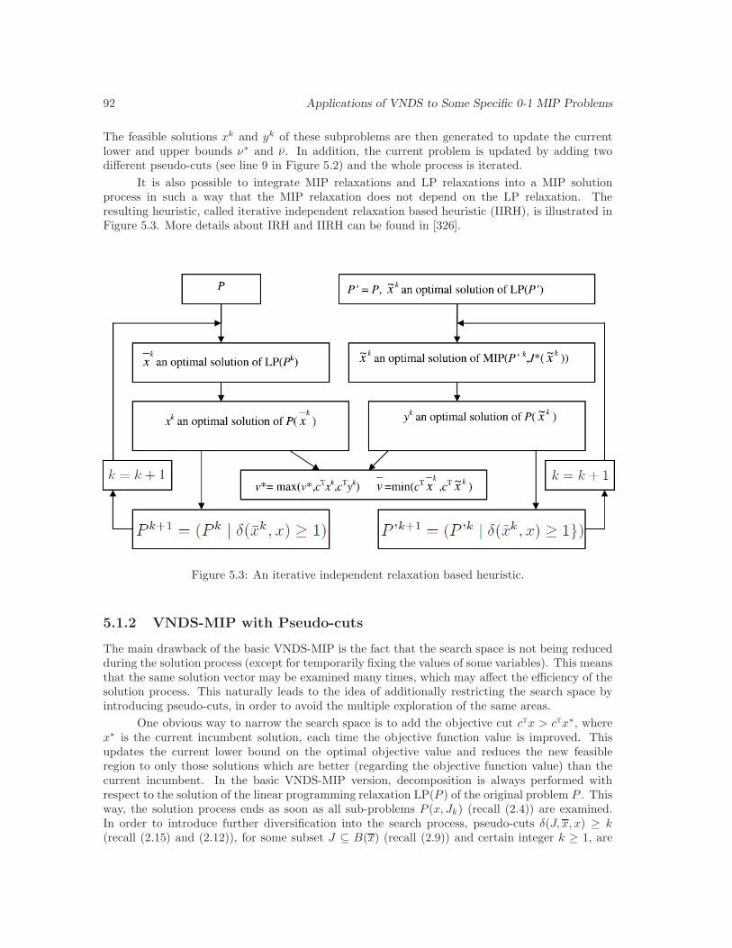
92 Applications of VNDS to Some Specific 0-1 MIP Problems
The feasible solutions xk and yk of these subproblems are then generated to update the currentlower and upper bounds ν∗ and ν. In addition, the current problem is updated by adding twodifferent pseudo-cuts (see line 9 in Figure 5.2) and the whole process is iterated.
It is also possible to integrate MIP relaxations and LP relaxations into a MIP solutionprocess in such a way that the MIP relaxation does not depend on the LP relaxation. Theresulting heuristic, called iterative independent relaxation based heuristic (IIRH), is illustrated inFigure 5.3. More details about IRH and IIRH can be found in [326].
Figure 5.3: An iterative independent relaxation based heuristic.
5.1.2 VNDS-MIP with Pseudo-cuts
The main drawback of the basic VNDS-MIP is the fact that the search space is not being reducedduring the solution process (except for temporarily fixing the values of some variables). This meansthat the same solution vector may be examined many times, which may affect the efficiency of thesolution process. This naturally leads to the idea of additionally restricting the search space byintroducing pseudo-cuts, in order to avoid the multiple exploration of the same areas.
One obvious way to narrow the search space is to add the objective cut ctx > ctx∗, wherex∗ is the current incumbent solution, each time the objective function value is improved. Thisupdates the current lower bound on the optimal objective value and reduces the new feasibleregion to only those solutions which are better (regarding the objective function value) than thecurrent incumbent. In the basic VNDS-MIP version, decomposition is always performed withrespect to the solution of the linear programming relaxation LP(P ) of the original problem P . Thisway, the solution process ends as soon as all sub-problems P (x, Jk) (recall (2.4)) are examined.In order to introduce further diversification into the search process, pseudo-cuts δ(J, x, x) ≥ k(recall (2.15) and (2.12)), for some subset J ⊆ B(x) (recall (2.9)) and certain integer k ≥ 1, are
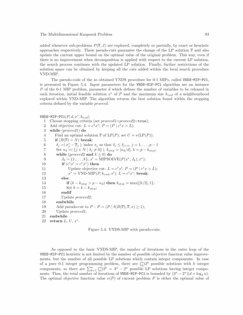
The Multidimensional Knapsack Problem 93
added whenever sub-problems P (x, J) are explored, completely or partially, by exact or heuristicapproaches respectively. These pseudo-cuts guarantee the change of the LP solution x and alsoupdate the current upper bound on the optimal value of the original problem. This way, even ifthere is no improvement when decomposition is applied with respect to the current LP solution,the search process continues with the updated LP solution. Finally, further restrictions of thesolution space can be obtained by keeping all the cuts added within the local search procedureVND-MIP.
The pseudo-code of the so obtained VNDS procedure for 0-1 MIPs, called VNDS-MIP-PC1,is presented in Figure 5.4. Input parameters for the VNDS-MIP-PC1 algorithm are an instanceP of the 0-1 MIP problem, parameter d which defines the number of variables to be released ineach iteration, initial feasible solution x∗ of P and the maximum size kvnd of a neighbourhoodexplored within VND-MIP. The algorithm returns the best solution found within the stoppingcriteria defined by the variable proceed.
VNDS-MIP-PC1(P, d, x∗, kvnd)1 Choose stopping criteria (set proceed1=proceed2=true);2 Add objective cut: L = ctx∗; P = (P | ctx > L).3 while (proceed1) do4 Find an optimal solution x of LP(P ); set U = ν(LP(P ));5 if (B(x) = N) break;6 δj =| x∗j − xj |; index xj so that δj ≤ δj+1, j = 1, . . . , p− 17 Set nd =| {j ∈ N | δj 6= 0} |, kstep = [nd/d], k = p− kstep;8 while (proceed2 and k ≥ 0) do9 Jk = {1, . . . , k}; x′ = MIPSOLVE(P (x∗, Jk), x∗);
10 if (ctx′ > ctx∗) then11 Update objective cut: L = ctx′; P = (P | ctx > L);12 x∗ = VND-MIP(P, kvnd, x′); L = ctx∗; break;13 else14 if (k − kstep > p− nd) then kstep = max{[k/2], 1};15 Set k = k − kstep;16 endif17 Update proceed2;18 endwhile19 Add pseudo-cut to P : P = (P | δ(B(x), x, x) ≥ 1);20 Update proceed1;21 endwhile22 return L, U , x∗.
Figure 5.4: VNDS-MIP with pseudo-cuts.
As opposed to the basic VNDS-MIP, the number of iterations in the outer loop of theVNDS-MIP-PC1 heuristic is not limited by the number of possible objective function value improve-ments, but the number of all possible LP solutions which contain integer components. In caseof a pure 0-1 integer programming problem, there are
(nk
)2k possible solutions with k integer
components, so there are∑n
k=1
(nk
)2k = 3n − 2n possible LP solutions having integer compo-
nents. Thus, the total number of iterations of VNDS-MIP-PC1 is bounded by (3n − 2n)(d + log2 n).The optimal objective function value ν(P ) of current problem P is either the optimal value of
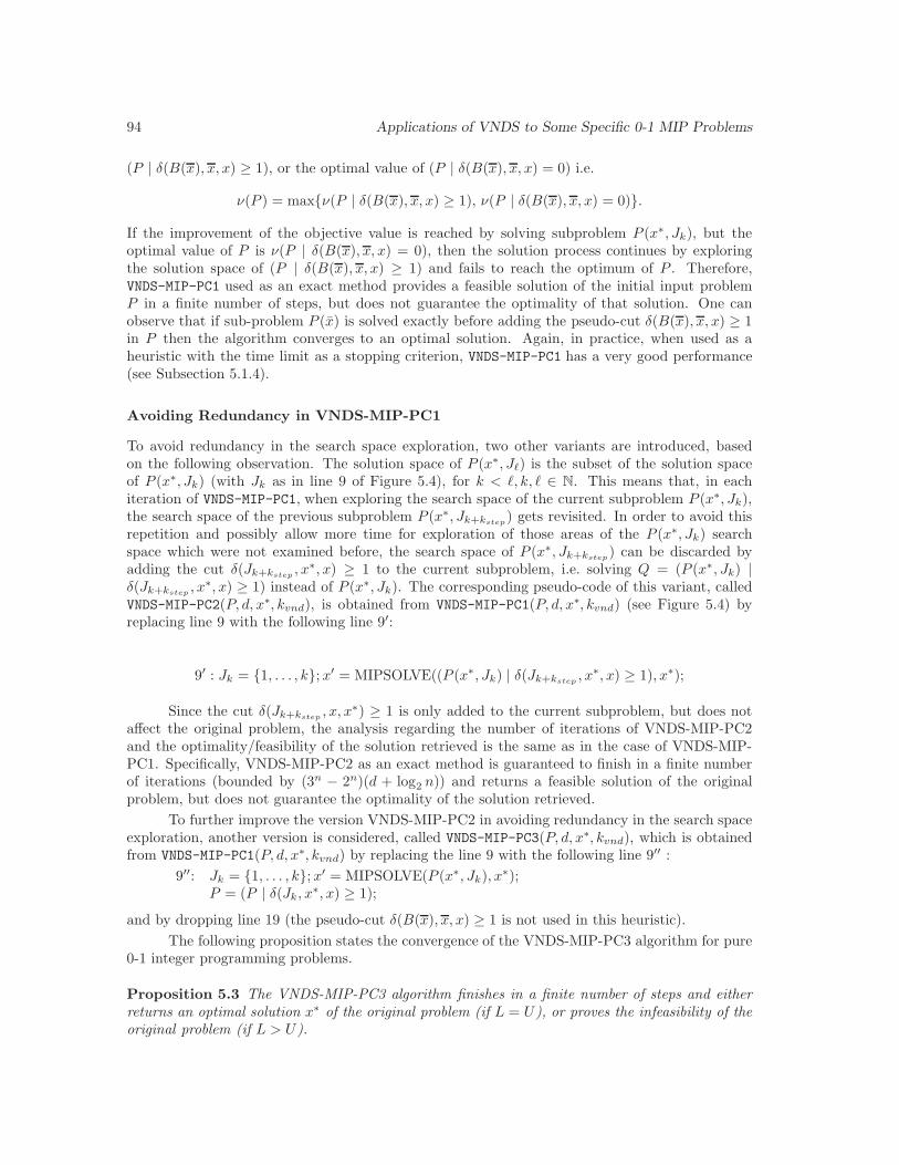
94 Applications of VNDS to Some Specific 0-1 MIP Problems
(P | δ(B(x), x, x) ≥ 1), or the optimal value of (P | δ(B(x), x, x) = 0) i.e.
ν(P ) = max{ν(P | δ(B(x), x, x) ≥ 1), ν(P | δ(B(x), x, x) = 0)}.
If the improvement of the objective value is reached by solving subproblem P (x∗, Jk), but theoptimal value of P is ν(P | δ(B(x), x, x) = 0), then the solution process continues by exploringthe solution space of (P | δ(B(x), x, x) ≥ 1) and fails to reach the optimum of P . Therefore,VNDS-MIP-PC1 used as an exact method provides a feasible solution of the initial input problemP in a finite number of steps, but does not guarantee the optimality of that solution. One canobserve that if sub-problem P (x) is solved exactly before adding the pseudo-cut δ(B(x), x, x) ≥ 1in P then the algorithm converges to an optimal solution. Again, in practice, when used as aheuristic with the time limit as a stopping criterion, VNDS-MIP-PC1 has a very good performance(see Subsection 5.1.4).
Avoiding Redundancy in VNDS-MIP-PC1
To avoid redundancy in the search space exploration, two other variants are introduced, basedon the following observation. The solution space of P (x∗, Jℓ) is the subset of the solution spaceof P (x∗, Jk) (with Jk as in line 9 of Figure 5.4), for k < ℓ, k, ℓ ∈ N. This means that, in eachiteration of VNDS-MIP-PC1, when exploring the search space of the current subproblem P (x∗, Jk),the search space of the previous subproblem P (x∗, Jk+kstep
) gets revisited. In order to avoid thisrepetition and possibly allow more time for exploration of those areas of the P (x∗, Jk) searchspace which were not examined before, the search space of P (x∗, Jk+kstep
) can be discarded byadding the cut δ(Jk+kstep
, x∗, x) ≥ 1 to the current subproblem, i.e. solving Q = (P (x∗, Jk) |δ(Jk+kstep
, x∗, x) ≥ 1) instead of P (x∗, Jk). The corresponding pseudo-code of this variant, calledVNDS-MIP-PC2(P, d, x∗, kvnd), is obtained from VNDS-MIP-PC1(P, d, x∗, kvnd) (see Figure 5.4) byreplacing line 9 with the following line 9′:
9′ : Jk = {1, . . . , k}; x′ = MIPSOLVE((P (x∗, Jk) | δ(Jk+kstep, x∗, x) ≥ 1), x∗);
Since the cut δ(Jk+kstep, x, x∗) ≥ 1 is only added to the current subproblem, but does not
affect the original problem, the analysis regarding the number of iterations of VNDS-MIP-PC2and the optimality/feasibility of the solution retrieved is the same as in the case of VNDS-MIP-PC1. Specifically, VNDS-MIP-PC2 as an exact method is guaranteed to finish in a finite numberof iterations (bounded by (3n − 2n)(d + log2 n)) and returns a feasible solution of the originalproblem, but does not guarantee the optimality of the solution retrieved.
To further improve the version VNDS-MIP-PC2 in avoiding redundancy in the search spaceexploration, another version is considered, called VNDS-MIP-PC3(P, d, x∗, kvnd), which is obtainedfrom VNDS-MIP-PC1(P, d, x∗, kvnd) by replacing the line 9 with the following line 9′′ :
9′′: Jk = {1, . . . , k}; x′ = MIPSOLVE(P (x∗, Jk), x∗);P = (P | δ(Jk, x∗, x) ≥ 1);
and by dropping line 19 (the pseudo-cut δ(B(x), x, x) ≥ 1 is not used in this heuristic).
The following proposition states the convergence of the VNDS-MIP-PC3 algorithm for pure0-1 integer programming problems.
Proposition 5.3 The VNDS-MIP-PC3 algorithm finishes in a finite number of steps and eitherreturns an optimal solution x∗ of the original problem (if L = U), or proves the infeasibility of theoriginal problem (if L > U).

The Multidimensional Knapsack Problem 95
Proof. The number of outer loop iterations of VNDS-MIP-PC3 is at most the number of all possibleincumbent integer solutions, which is not greater than 2n (because the cut δ(Jk, x∗, x) > 1 enforcesthe change of incumbent integer solution in each iteration, except when Jk = ∅). When Jk = ∅,all possible integer solution vectors have been examined. The number of inner loop iterations isbounded by d + log2 n, so the total number of iterations is at most 2n(d + log2 n).
The pseudo-cut δ(Jk, x∗, x) ≥ 1 does not necessarily change the optimal value of the LPrelaxation of P at each iteration. However, we have that P (x∗, Jk) = (P | δ(Jk, x∗, x) = 0) andν(P ) = max{ν((P | δ(Jk, x∗, x) ≥ 1)), ν((P | δ(Jk, x∗, x) = 0))}. So, if the optimal solution of thereduced problem P (x∗, Jk) is not optimal for P , then the cut δ(Jk, x∗, x) ≥ 1 does not discard theoptimal value of the original problem P . We have already proved that this algorithm finishes ina finite number of steps, so it follows that it either returns an optimal solution x∗ of the originalproblem (if L = U), or proves the infeasibility of the original problem (if L > U). �
Different Ordering Strategies.
In the VNDS-MIP variants discussed so far, variables in the incumbent integer solution wereordered according to the distances of their values to the values of the current linear programmingrelaxation solution. However, it is possible to employ different ordering strategies. For example,consider the following two problems:
(LP−
x∗)
2
6
6
4
min δ(x∗, x)s.t.: Ax ≤ b
ctx ≥ L + 1xj ∈ [0, 1] , j ∈ N
(LP+
x∗)
2
6
6
4
max δ(x∗, x)s.t.: Ax ≤ b
ctx ≥ L + 1xj ∈ [0, 1] , j ∈ N
where x∗ is the incumbent integer feasible solution and L is the best lower bound found so far(i.e., L = ctx∗). If x− and x+ are optimal solutions of LP relaxation problems LP−x∗ and LP+
x∗ ,respectively, then components of x∗ could be ordered in ascending order of values |x−j − x+
j |,
j ∈ N . Since both solution vectors x− and x+ are real-valued (i.e. from Rn), this orderingtechnique is expected to be more sensitive than the standard one, i.e. the number of pairs (j, j′),j, j′ ∈ N, j 6= j′ for which |x−j − x+
j | 6= |x−j′ − x+
j′ | is expected to be greater than the number ofpairs (h, h′), h, h′ ∈ N, h 6= h′ for which |x∗h − xh| 6= |x∗h′ − xh′ |, where x is an optimal solution ofthe LP relaxation LP (P ). Also, according to the definition of x− and x+, it is intuitively morelikely that the variables xj , j ∈ N , for which x−j = x+
j , will have that same value x−j in the final
solution, than it is for variables xj , j ∈ N , for which x∗j = xj (and x−j 6= x+j ), to have the final
value x∗j . In practice, if x−j = x+j , j ∈ N , then usually x∗j = x−j , which justifies the ordering of
components of x∗ in the described way. However, if we want to keep the number of iterations in onepass of VNDS-MIP approximately the same as in the standard ordering, i.e. if we want to use thesame value for parameter d, then the subproblems examined will be larger than with the standardordering, since the value of nd will be smaller (see line 7 of Figure 5.4). The pseudo-code of thisvariant of VNDS-MIP, called VNDS-MIP-PC4, is provided in Figure 5.5. It is easy to prove thatVNDS-MIP-PC4 used as an exact method provides a feasible solution of the initial input problemP in a finite number of steps, but does not guarantee the optimality of that solution. As in thecase of VNDS-MIP-PC1, one can observe that if subproblems P (x+) and P (x−) are solved exactlybefore adding pseudo-cuts δ(B(x+), x+, x) ≥ 1 and δ(B(x−), x−, x) ≥ 1 to P , then the algorithmconverges to an optimal solution.

96 Applications of VNDS to Some Specific 0-1 MIP Problems
VNDS-MIP-PC4(P, d, x∗, kvnd)1 Choose stopping criteria (set proceed1=proceed2=true);2 Add objective cut: L = ctx∗; P = (P | ctx > L).3 while (proceed1) do4 Find an optimal solution x of LP(P ); set U = ν(LP(P ));5 if (B(x) = N) break;6 Find optimal solutions x− of LP−x∗ and x+ of LP+
x∗ ;7 δj =| x−j − x+
j |; index xj so that δj ≤ δj+1
8 Set nd =| {j ∈ N | δj 6= 0} |, kstep = [nd/d], k = p− kstep;9 while (proceed2 and k ≥ 0) do
10 Jk = {1, . . . , k}; x′ = MIPSOLVE(P (x∗, Jk), x∗);P = (P | δ(Jk, x∗, x) ≥ 1);11 if (ctx′ > ctx∗) then12 Update objective cut: L = ctx′; P = (P | ctx > L);13 x∗ = VND-MIP(P, kvnd, x′); L = ctx∗; break;14 else15 if (k − kstep > p− nd) then kstep = max{[k/2], 1};16 Set k = k − kstep;17 endif18 Update proceed2;19 endwhile20 Add pseudo-cuts to P : P = (P | {δ(B(x+), x+, x) ≥ 1, δ(B(x−), x−, x) ≥ 1});21 Update proceed1;22 endwhile23 return L, U , x∗.
Figure 5.5: VNDS-MIP with upper and lower bounding and another ordering strategy.
5.1.3 A Second Level of Decomposition in VNDS
In this section we propose the use of a second level of decomposition in VNDS for the MKP. TheMKP is tackled by decomposing the problem to several subproblems where the number of itemsto choose is fixed to a given integer value. Fixing the number of items in a knapsack to a givenvalue h ∈ N∪{0} can be achieved by adding the constraint x1 +x2 + . . .+xn = h, or, equivalently,etx = h, where e is the vector of 1s.
Formally, let Ph be a subproblem obtained from the original problem by adding the hyper-plane constraint etx = h for h ∈ N and enriched by an objective cut, defined as follows:
(Ph)
max ctxs.t.: Ax ≤ b
ctx ≥ L + 1etx = hx ∈ {0, 1}n
Solving the MKP by tackling separately each of the subproblems Ph for h ∈ N appeared tobe an interesting approach [41, 310, 311, 314] especially because the additional constraint (etx = h)provides tighter upper bounds than the classical LP relaxation.
Let hmin and hmax denote lower and upper bounds of the number of variables with value1 in an optimal solution of the problem. Then it is obvious that ν(P ) = max{ν(Ph) | hmin ≤h ≤ hmax}. Bounds hmin =
⌈ν(LP−0 )
⌉and hmax =
⌊ν(LP+
0 )⌋
can be computed by solving the
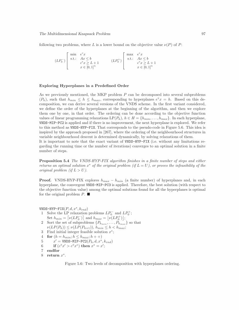
The Multidimensional Knapsack Problem 97
following two problems, where L is a lower bound on the objective value ν(P ) of P :
(LP−
0 )
2
6
6
4
min etx
s.t.: Ax ≤ b
ctx ≥ L + 1x ∈ [0, 1]n
(LP+
0 )
2
6
6
4
max etx
s.t.: Ax ≤ b
ctx ≥ L + 1x ∈ [0, 1]n
Exploring Hyperplanes in a Predefined Order
As we previously mentioned, the MKP problem P can be decomposed into several subproblems(Ph), such that hmin ≤ h ≤ hmax, corresponding to hyperplanes etx = h. Based on this de-composition, we can derive several versions of the VNDS scheme. In the first variant considered,we define the order of the hyperplanes at the beginning of the algorithm, and then we explorethem one by one, in that order. The ordering can be done according to the objective functionvalues of linear programming relaxations LP(Ph), h ∈ H = {hmin, . . . , hmax}. In each hyperplane,VNDS-MIP-PC2 is applied and if there is no improvement, the next hyperplane is explored. We referto this method as VNDS-HYP-FIX. That corresponds to the pseudo-code in Figure 5.6. This idea isinspired by the approach proposed in [267], where the ordering of the neighbourhood structures invariable neighbourhood descent is determined dynamically, by solving relaxations of them.It is important to note that the exact variant of VNDS-HYP-FIX (i.e. without any limitations re-garding the running time or the number of iterations) converges to an optimal solution in a finitenumber of steps.
Proposition 5.4 The VNDS-HYP-FIX algorithm finishes in a finite number of steps and eitherreturns an optimal solution x∗ of the original problem (if L = U), or proves the infeasibility of theoriginal problem (if L > U).
Proof. VNDS-HYP-FIX explores hmax − hmin (a finite number) of hyperplanes and, in eachhyperplane, the convergent VNDS-MIP-PC3 is applied. Therefore, the best solution (with respect tothe objective function value) among the optimal solutions found for all the hyperplanes is optimalfor the original problem P . �
VNDS-HYP-FIX(P, d, x∗, kvnd)1 Solve the LP relaxation problems LP−0 and LP+
0 ;Set hmin =
⌈ν(LP−0 )
⌉and hmax =
⌊ν(LP+
0 )⌋;
2 Sort the set of subproblems {Phmin, . . . , Phmax
} so thatν(LP (Ph)) ≤ ν(LP (Ph+1)), hmin ≤ h < hmax;
3 Find initial integer feasible solution x∗;4 for (h = hmin; h ≤ hmax; h + +)5 x′ = VNDS-MIP-PC2(Ph, d, x∗, kvnd)6 if (ctx′ > ctx∗) then x∗ = x′;7 endfor8 return x∗.
Figure 5.6: Two levels of decomposition with hyperplanes ordering.

98 Applications of VNDS to Some Specific 0-1 MIP Problems
Flexibility in Changing Hyperplanes
In the second variant we consider the hyperplanes in the same order as in the previous version.However, instead of changing the hyperplane only when the current one is completely explored,the change is allowed depending on other conditions (a given running time, a number of itera-tions without improving the current best solution, . . . ). Figure 5.7 provides a description of thisalgorithm, called VNDS-HYP-FLE, in which proceed3 corresponds to the condition for changing thehyperplane.
In this algorithm, we simply increase the value of h by one when the changing condition issatisfied; in case when h = hmax, h is fixed to the first possible value starting from hmin. Whenthe best solution is improved, the values of hmin and hmax are also recomputed and the set H isupdated if necessary (line 15 in Figure 5.7). In the same way, if a hyperplane is completely explored(or if it is proved not to contain an optimal solution) the set H is updated and the value of h ischanged (line 8 in Figure 5.7). The condition proceed3 corresponds to a maximum running timefixed according to the size of the problem (see Subsection 5.1.4 for more details about parameters).It is easy to see that VNDS-HYP-FLE is not guaranteed to find an optimal solution of the inputproblem.
5.1.4 Computational Results
All values presented in this section are obtained using a Pentium 4 computer with 3.4GHz proces-sor and 4GB RAM and general purpose MIP solver CPLEX 11.1 [183]. The C++ programminglanguage was used to code the algorithms, which were compiled with g++ and the option -O2.
Test Bed
The proposed heuristics are validated on two sets of available and correlated instances of MKP.The first set is composed by 270 instances with n = 100, 250 and 500, and m = 5, 10, 30. Theseinstances are grouped in the OR-Library, and the larger instances with n = 500 are known tobe difficult. So we test our methods over the 90 instances with n = 500. In particular the opti-mal solutions of the instances with m = 30 are not known, whereas the running time needed toprove the optimality of the solutions for the instances with m = 10 is in general very important [41].
The second set of instances is composed by 18 MKP problems generated by [127], withnumber of items n between 100 and 2500, and number of knapsack constraints m between 15 and100. We selected these problems because they are known to be very hard to solve by branch-and-bound technique.
Parameter Settings
As mentioned earlier, the CPLEX MIP solver is used in each method compared. We now give moredetailed explanation how we use its parameters. We choose to set the CPX PARAM MIP EMPHASIS
to FEASIBILITY for the first feasible solution, and then change to the default BALANCED optionafter the first feasible solution has been found.
Several variants of our heuristics use the same parameters. In all the cases we set the valueof parameter d to 10, and we set kvnd = 5. Furthermore, we allow running time tsub = tvnd = 300s

The Multidimensional Knapsack Problem 99
VNDS-HYP-FLE(P, d, x∗, kvnd)1 Solve the LP relaxation problems LP−0 and LP+
0 ;set hmin =
⌈ν(LP−0 )
⌉and hmax =
⌊ν(LP+
0 )⌋;
2 Sort the set of subproblems {Phmin, . . . , Phmax
} so thatν(LP (Ph)) ≤ ν(LP (Ph+1)), hmin ≤ h < hmax;
3 Find an initial integer feasible solution x∗; L = ctx∗;4 Choose stopping criteria (set proceed1=proceed2=proceed3=true) ;5 Set h = hmin and P = Ph;6 while (proceed1)7 Find an optimal solution x of LP(P ); U = min{U, ν(LP(P ))};8 if (cTx∗ ≥ cTx or B(x) = N) then H = H − {h} ;
Choose the next value h in H and Set P = Ph;9 δj =| x∗j − xj |; index xj so that δj ≤ δj+1
10 Set nd =| {j ∈ N | δj 6= 0} |, kstep = [nd/d], k = p− kstep;11 while (proceed2 and k ≥ 0)12 Jk = {1, . . . , k}; x′ = MIPSOLVE(P (x∗, Jk), x∗);13 if (ctx′ > ctx∗) then14 Update objective cut: L = ctx′; P = (P | ctx > L);15 Recompute hmin, hmax and update H , h and P if necessary;16 x∗ = VND-MIP(P, kvnd, x′); L = ctx∗; break;17 else18 if (k − kstep > p− nd) then kstep = max{[k/2], 1};19 Set k = k − kstep;20 endif21 Update proceed3;22 if (proceed3=false) then
proceed3=true; goto 26;23 Update proceed2;24 endwhile25 Add pseudo-cut to P : P = (P | δ(B(x), x, x) ≥ 1);26 Update proceed1.27 endwhile28 return L, U , x∗.
Figure 5.7: Flexibility for changing the hyperplanes.
for calls to the CPLEX MIP solver for subproblems and calls to VND, respectively, for all instancesin the test bed, unless otherwise specified. Finally, the running time limit is set to 1 hour (3,600seconds) for each instance. VNDS-HYP-FLE has another parameter that corresponds to the run-ning time before changing the value of σ (condition proceed3 in Figure 5.7). In our experimentsthis value is fixed at 900s (according to preliminary experiments).
Comparison
In Tables 5.1-5.3, the results obtained by all variants over the instances with n = 500 andm = 5, 10, 30 respectively, are provided. These values were obtained by several recent hybridmethods (see [41, 154, 311, 314, 326]). In these tables, in column “Best” the optimal value (or thebest-known lower bound for m = 30) is reported. Then, for each variant, the difference between

100 Applications of VNDS to Some Specific 0-1 MIP Problems
this best value and the value obtained by the observed heuristic is reported, as well as the CPUtime to reach this value.
Table 5.1 shows that the proposed heuristics obtain good results over these instances, exceptfor VNDS-HYP-FIX that visits only 3 optimal solutions. However, for m = 5 and m = 10 VNDS-HYP-FIX reaches good quality near-optimal solutions in much shorter time than other methodsobserved. The results for all variants are very similar, in particular for the average gap less than0.001% (between 23 and 30 optimal solutions). One can also observe that VNDS-MIP slightlydominates the other variants in term of average running time needed to visit the optimal solutions,and that VNDS-HYP-FLE visits all the optimal solutions for these 30 instances. These results con-firm the potential of VNDS for solving the MKP. Another encouraging point is the good behaviourof VNDS-HYP-FLE, which confirms the interest of using the hyperplane decomposition, even ifthe use of this decomposition seems to be sensitive (according to the results of VNDS-HYP-FIX).Finally, the VNDS-MIP-PC3 proves the optimality of the solution obtained for the instance 5.500.1(the value is referred by a “*” in the table).
Table 5.2 shows that the behaviour of the heuristics is more different for larger instances.Globally the results confirm the efficiency of VNDS-MIP, even if it visits only 2 optimal solutions.VNDS-MIP-PC1 obtains interesting results with 6 optimal solutions and an average gap less than0.01. That illustrates the positive impact of the upper and lower bounding in the VNDS scheme.That is also confirmed by the results of VNDS-MIP-PC2 with the visit of 5 optimal solutions andthe same average gap. However the addition of the bouding method in these variants increasesthe average running time to reach the best solutions. The results obtained by VNDS-HYP-FIXconfirm that this variant converges quickly to good solutions of MKP, but, in general, it soon getsstalled in the local optimum encountered during the search, due to the long computational timeneeded for exploration of particular hyperplanes. More precisely, since hyperplanes are exploredsuccessively, it is possible to explore only the first few hyperplanes within the CPU time allowed.Finally the VNDS-HYP-FLE is less efficient than for the previous instances. The increase of theCPU* can be easily explained by the fact that the hyperplane are explored iteratively. The qualityof the lower bound can also be explained by the fact that the “good” hyperplanes can be exploredinsufficiently. However these results are still encouraging.
The results obtained for the largest instances with m = 30 are more difficult to analyse.Indeed, the values reported in Table 5.3 do not completely confirm the previous results. In partic-ular we can observe that VNDS-MIP-PC3 is the “best” heuristic, if we consider only the averagegap. In addition, the associated running time is not significantly greater than the running timeof VNDS-MIP. It seems that, for these very difficult instances, the search space restrictions intro-duced in this heuristic have a positive effect over the VNDS scheme. The VNDS-MIP-PC4 is themost efficient heuristic if we consider only the number of best-known lower bounds visited. So,the other ordering strategy considered in this version, which can be considered as a diversificationmechanism when compared to the other versions, conducts the search in promising regions for theseinstances. Finally, the methods based on the hyperplane decomposition are less efficient for theselarge instances, as expected. That confirms the previous conclusions for m = 10 that it is difficultto quickly explore all hyperplanes or perform a good selection of hyperplanes to be explored in anefficient way.
In Table 5.4, we provide the average results obtained by the proposed heuristics over theOR-Library instances. For each heuristic we report the average gap obtained for all objectivevalues, and the number of optimal solutions (or best-known solutions) visited during the process.

The Multidimensional Knapsack Problem 101
The value α ∈ {0.25, 0.5, 0.75} was used to generate the instances according to the procedure in[110], and it corresponds to the correlation degree of the instances. There are 10 instances availablefor each (n, m, α) triplet. The main conclusions of this table can be listed as follows:
• According to the average gap, the VNDS-MIP-PC3 (very) slightly dominates the other vari-ants based on VNDS-MIP. Globally, it is difficult to distinguish one version from the others.
• The VNDS-HYP-* are clearly dominated in average, but not clearly for m = 10 (in particularfor VNDS-HYP-FLE and α > 0.5).
• The VNDS-HYP-FLE obtains most optimal solutions, thanks to very good results for m = 5and m = 10, α = 0.5.
• All the variants have difficulties in tackling the largest instances with m = 30. However, if1 hour of running time can be considered as an important value for heuristic approaches,it is necessary to observe that a large part of the optimal values and best-known values forthe instances with m = 10 and m = 30, respectively, were obtained in a significantly shortrunning time (see for instance [41, 314, 326].
According to the last remark, in Table 5.5 the average results obtained by the proposedheuristics with the running time limit set to 2 hours are reported. The results provided in thistable are interesting since they show that if we increase the running time, then VNDS-MIP-PC1dominates more clearly the VNDS-MIP heuristic, in particular for the instances with m = 30. Thatconfirms the potential of the bounding approach. In addition, the results obtained by VNDS-MIP-PC4 are also really improved, confirming the interest in changing the ordering strategy for largerinstances (with a larger running time). Globally the results of all the variants are clearly improved,in particular for m = 30 and α < 0.75. Finally, a “*” is added for VNDS-MIP-PC1 and VNDS-MIP-PC4 when m = 30 and α = 0.25 since these two variants visit one new best known solutionfor the instance 30.500-3 with an objective value equal to 115,370.
Tables 5.6-5.7 are devoted to the results obtained over the second data set of instances. Ta-ble 5.6 provides the overall results for all the heuristics compared to the best-known lower boundsreported in column “Best”. These values were obtained by an efficient hybrid tabu search algo-rithm [310] and by the iterative heuristics proposed by Hanafi and Wilbaut [326]. Due to the largesize of several instances and the long running time needed by the other approaches to obtain thebest-known solutions, two different values for the running time of the proposed heuristics are used.The running time limit is set to 5 hours for the instances MK GK04, MK GK06 and MK GK08-MK GK11, and to 2 hours for all other MK GK instances.
Table 5.6 demonstrates the global interesting behaviour of the proposed heuristics, whichreach a significant number of best-known solutions and also two new best solutions. In general,the new versions derived from VNDS-MIP with some new modifications converge more quickly tothe best solutions. That is particularly the case for the VNDS-MIP-PC1, VNDS-MIP-PC2 andVNDS-MIP-PC3. In average, we can observe that VNDS-MIP-PC1 obtains the best results. Theprevious conclusions about the hyperplane-based heuristics are still valid: the flexible scheme ismore efficient for the medium size instances. However, for these instances the results obtained byVNDS-HYP-FIX are more encouraging, with the visit of a new best lower bound and the conver-gence to good lower bounds for the larger instances.

102
Applica
tions
ofV
ND
Sto
Som
eSpecifi
c0-1
MIP
Pro
blem
s
VNDS-MIP VNDS-MIP-PC1 VNDS-MIP-PC2 VNDS-MIP-PC3 VNDS-MIP-PC4 VNDS-HYP-FIX VNDS-HYP-FLEinst. Best Best-lb CPU* Best-lb CPU* Best-lb CPU* Best-lb CPU* Best-lb CPU* Best-lb CPU* Best-lb CPU*
5.500-0 120148 0 1524 3 794 0 2497 5 984 5 2859 38 120 0 12355.500-1 117879 0 138 0 475 0 525 0* 2663 16 2722 35 477 0 5905.500-2 121131 0 2131 2 80 0 1999 0 2920 0 2524 47 167 0 4845.500-3 120804 0 1703 5 3006 5 2807 5 2259 0 3138 17 373 0 31925.500-4 122319 0 93 0 7 0 203 0 303 0 240 0 35 0 3235.500-5 122024 0 722 0 7 0 19 0 43 13 666 37 55 0 1125.500-6 119127 0 580 0 2010 0 3195 0 2068 0 2567 20 538 0 3225.500-7 120568 0 167 0 615 0 1067 0 1152 0 72 32 33 0 5355.500-8 121586 0 1670 0 2820 11 1104 11 1109 11 209 18 222 0 9015.500-9 120717 0 868 13 2943 6 3389 0 984 0 798 45 3458 0 3198
5.500-10 218428 0 170 0 316 0 648 0 12 3 1982 6 3211 0 11685.500-11 221202 0 704 0 356 0 435 0 1508 0 122 11 27 0 9425.500-12 217542 0 1957 6 0 6 106 0 2341 0 389 0 2 0 18355.500-13 223560 0 89 0 10 0 236 0 133 0 738 26 16 0 3015.500-14 218966 0 88 0 332 0 353 0 310 0 559 4 5 0 1555.500-15 220530 0 1265 0 1562 0 953 0 1360 3 2417 44 3091 0 20755.500-16 219989 0 7 0 7 0 26 0 24 0 71 51 56 0 7835.500-17 218215 0 1230 0 1875 0 1944 0 2391 0 91 35 812 0 7745.500-18 216976 0 7 0 25 0 101 0 12 0 60 24 47 0 2445.500-19 219719 0 457 0 437 0 648 0 833 0 1035 21 31 0 4235.500-20 295828 0 5 0 5 0 47 0 71 0 28 40 135 0 17715.500-21 308086 0 2 0 235 0 268 0 162 3 855 20 226 0 285.500-22 299796 0 3 0 176 0 180 0 57 0 240 29 209 0 805.500-23 306480 0 2078 0 20 0 33 4 5 0 1041 11 81 0 355.500-24 300342 0 1 0 185 0 199 0 26 0 252 0 87 0 7775.500-25 302571 0 1097 6 3076 0 1782 0 1625 0 909 22 40 0 1335.500-26 301339 0 366 0 1355 0 1333 0 908 0 220 30 213 0 7355.500-27 306454 0 366 0 1041 0 1183 0 524 0 759 32 11 0 2125.500-28 302828 0 466 0 716 0 782 0 719 0 310 61 10 0 5495.500-29 299910 4 0 4 16 6 28 4 67 0 281 29 51 0 2209
Avg. CPU* 665 817 936 919 938 461 871Avg. Gap <0.001 <0.001 <0.001 <0.001 <0.001 <0.001 0
#opt 29 23 25 25 23 3 30
Table 5.1: Results for the 5.500 instances.

The
Multid
imen
sionalK
napsa
ckP
roblem
103
VNDS-MIP VNDS-MIP-PC1 VNDS-MIP-PC2 VNDS-MIP-PC3 VNDS-MIP-PC4 VNDS-HYP-FIX VNDS-HYP-FLEinst. Best Best-lb CPU* Best-lb CPU* Best-lb CPU* Best-lb CPU* Best-lb CPU* Best-lb CPU* Best-lb CPU*
10.500-0 117821 12 326 21 1582 12 1580 12 419 42 1417 110 606 12 304410.500-1 119249 32 38 32 3547 32 847 32 348 49 2178 109 300 83 271110.500-2 119215 4 986 4 1163 4 2920 4 558 4 152 71 300 0 184710.500-3 118829 16 613 16 1867 16 2166 16 2006 16 611 54 399 16 195910.500-4 116530 21 27 21 1227 21 1527 50 1828 39 2992 89 917 37 274810.500-5 119504 14 852 25 1469 14 1170 14 1885 25 1364 91 300 43 36410.500-6 119827 62 2411 14 911 37 606 55 1812 43 995 64 300 50 349410.500-7 118344 15 2409 21 2271 32 2870 32 1299 35 1728 98 919 11 348510.500-8 117815 39 3029 0 1233 34 2056 36 3338 39 378 27 454 39 60010.500-9 119251 48 1231 33 1531 28 3332 44 3166 0 399 67 351 97 1825
10.500-10 217377 20 2315 0 1257 0 1557 0 1213 28 1111 43 2476 0 339910.500-11 219077 14 2721 16 2032 14 1999 11 3025 19 3060 57 901 14 128110.500-12 217847 50 1846 50 2447 0 2746 50 1404 0 211 92 26 0 181410.500-13 216868 0 63 0 93 0 393 0 363 17 904 0 69 0 152810.500-14 213873 14 1843 14 689 14 388 14 958 20 768 65 425 30 122510.500-15 215086 24 2579 24 1502 0 3002 50 1815 1 1944 11 430 0 110810.500-16 217940 33 2476 42 1042 9 3443 9 1496 9 3505 52 305 42 66310.500-17 219990 6 2468 6 2154 6 1554 6 1475 21 2137 51 370 41 195410.500-18 214382 36 1932 27 3002 7 2402 30 3385 16 756 50 431 31 38310.500-19 220899 27 877 17 1978 17 3191 27 1682 12 3188 63 334 27 328910.500-20 304387 37 1990 0 2218 24 3206 28 582 28 1665 49 302 34 184110.500-21 302379 32 2628 0 2000 23 3016 0 2113 21 1038 34 345 38 165010.500-22 302417 1 1824 1 2766 1 3041 8 1372 1 636 66 351 17 60510.500-23 300784 27 2287 41 952 39 1226 41 1373 37 41 46 195 27 307210.500-24 304374 0 1258 0 1771 7 3577 8 2281 8 3575 33 182 17 345610.500-25 301836 40 1285 55 2174 40 1691 40 3112 40 3540 0 3509 40 257810.500-26 304952 3 663 3 1401 2 1391 1 393 0 411 3 1 7 150110.500-27 296478 12 717 12 2742 22 1234 12 3037 21 3349 68 335 22 225810.500-28 301359 2 2203 6 1044 2 1936 6 1601 15 489 44 358 6 181410.500-29 307089 17 1039 17 1044 0 1640 11 2475 0 724 51 102 17 1307
Avg. CPU* 1564 1703 2057 1727 1508 543 1960Avg. Gap 0.013 0.009 0.009 0.013 0.012 0.034 0.016
#opt 2 6 5 3 4 2 5
Table 5.2: Results for the 10.500 instances.
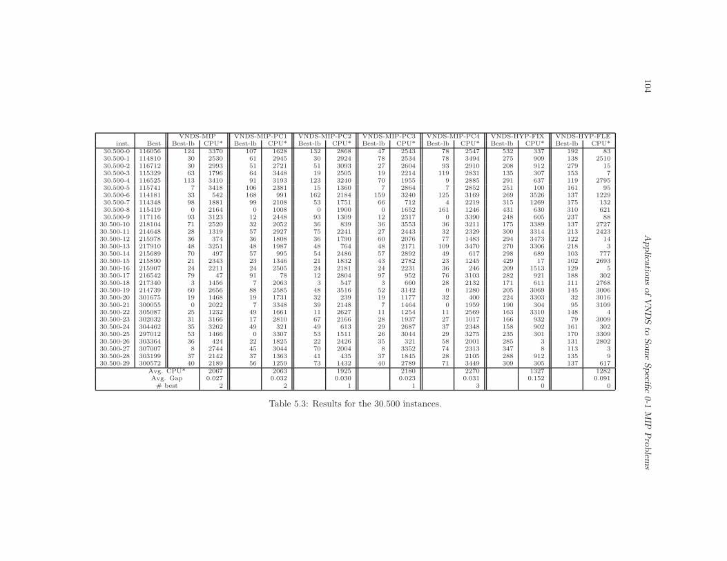
104
Applica
tions
ofV
ND
Sto
Som
eSpecifi
c0-1
MIP
Pro
blem
s
VNDS-MIP VNDS-MIP-PC1 VNDS-MIP-PC2 VNDS-MIP-PC3 VNDS-MIP-PC4 VNDS-HYP-FIX VNDS-HYP-FLEinst. Best Best-lb CPU* Best-lb CPU* Best-lb CPU* Best-lb CPU* Best-lb CPU* Best-lb CPU* Best-lb CPU*
30.500-0 116056 124 3370 107 1628 132 2868 47 2543 78 2547 532 337 192 8330.500-1 114810 30 2530 61 2945 30 2924 78 2534 78 3494 275 909 138 251030.500-2 116712 30 2993 51 2721 51 3093 27 2604 93 2910 208 912 279 1530.500-3 115329 63 1796 64 3448 19 2505 19 2214 119 2831 135 307 153 730.500-4 116525 113 3410 91 3193 123 3240 70 1955 9 2885 291 637 119 279530.500-5 115741 7 3418 106 2381 15 1360 7 2864 7 2852 251 100 161 9530.500-6 114181 33 542 168 991 162 2184 159 3240 125 3169 269 3526 137 122930.500-7 114348 98 1881 99 2108 53 1751 66 712 4 2219 315 1269 175 13230.500-8 115419 0 2164 0 1008 0 1900 0 1652 161 1246 431 630 310 62130.500-9 117116 93 3123 12 2448 93 1309 12 2317 0 3390 248 605 237 88
30.500-10 218104 71 2520 32 2052 36 839 36 3553 36 3211 175 3389 137 272730.500-11 214648 28 1319 57 2927 75 2241 27 2443 32 2329 300 3314 213 242330.500-12 215978 36 374 36 1808 36 1790 60 2076 77 1483 294 3473 122 1430.500-13 217910 48 3251 48 1987 48 764 48 2171 109 3470 270 3306 218 330.500-14 215689 70 497 57 995 54 2486 57 2892 49 617 298 689 103 77730.500-15 215890 21 2343 23 1346 21 1832 43 2782 23 1245 429 17 102 269330.500-16 215907 24 2211 24 2505 24 2181 24 2231 36 246 209 1513 129 530.500-17 216542 79 47 91 78 12 2804 97 952 76 3103 282 921 188 30230.500-18 217340 3 1456 7 2063 3 547 3 660 28 2132 171 611 111 276830.500-19 214739 60 2656 88 2585 48 3516 52 3142 0 1280 205 3069 145 300630.500-20 301675 19 1468 19 1731 32 239 19 1177 32 400 224 3303 32 301630.500-21 300055 0 2022 7 3348 39 2148 7 1464 0 1959 190 304 95 310930.500-22 305087 25 1232 49 1661 11 2627 11 1254 11 2569 163 3310 148 430.500-23 302032 31 3166 17 2810 67 2166 28 1937 27 1017 166 932 79 300930.500-24 304462 35 3262 49 321 49 613 29 2687 37 2348 158 902 161 30230.500-25 297012 53 1466 0 3307 53 1511 26 3044 29 3275 235 301 170 330930.500-26 303364 36 424 22 1825 22 2426 35 321 58 2001 285 3 131 280230.500-27 307007 8 2744 45 3044 70 2004 8 3352 74 2313 347 8 113 330.500-28 303199 37 2142 37 1363 41 435 37 1845 28 2105 288 912 135 930.500-29 300572 40 2189 56 1259 73 1432 40 2789 71 3449 309 305 137 617
Avg. CPU* 2067 2063 1925 2180 2270 1327 1282Avg. Gap 0.027 0.032 0.030 0.023 0.031 0.152 0.091
# best 2 2 1 1 3 0 0
Table 5.3: Results for the 30.500 instances.

The
Multid
imen
sionalK
napsa
ckP
roblem
105
5.500 10.500 30.500α 0.25 0.5 0.75 0.25 0.5 0.75 0.25 0.5 0.75 Avg.
VNDS-MIP 0 0 <0.001 0.022 0.010 0.006 0.051 0.020 0.009 0.013VNDS-MIP-PC1 0.002 <0.001 <0.001 0.016 0.009 0.004 0.066 0.021 0.010 0.014VNDS-MIP-PC2 0.002 <0.001 <0.001 0.019 0.003 0.005 0.059 0.017 0.015 0.013
Avg. VNDS-MIP-PC3 0.002 0 <0.001 0.025 0.009 0.005 0.042 0.021 0.008 0.012Gap VNDS-MIP-PC4 0.004 <0.001 <0.001 0.025 0.007 0.006 0.058 0.022 0.012 0.015
VNDS-HYP-FIX 0.002 0.01 0.001 0.066 0.022 0.013 0.256 0.122 0.078 0.067VNDS-HYP-FLE 0 <0.001 0 0.033 0.009 0.007 0.164 0.068 0.040 0.036
Total
#opt
VNDS-MIP 10 10 9 0 1 1 1 0 1 33VNDS-MIP-PC1 6 9 8 1 2 3 1 0 1 31VNDS-MIP-PC2 7 9 9 0 4 1 1 0 0 31VNDS-MIP-PC3 7 10 8 0 2 1 1 0 0 29VNDS-MIP-PC4 6 8 9 1 1 2 1 1 1 30VNDS-HYP-FIX 1 1 1 0 1 1 0 0 0 5VNDS-HYP-FLE 10 10 10 1 4 0 0 0 0 35
Table 5.4: Average results on the OR-Library.
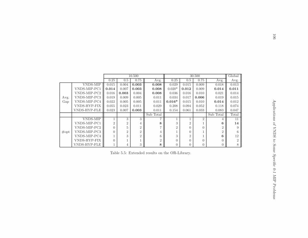
106
Applica
tions
ofV
ND
Sto
Som
eSpecifi
c0-1
MIP
Pro
blem
s
10.500 30.500 Global0.25 0.5 0.75 Avg. 0.25 0.5 0.75 Avg. Avg.
VNDS-MIP 0.015 0.004 0.003 0.008 0.029 0.015 0.009 0.018 0.013VNDS-MIP-PC1 0.014 0.007 0.003 0.008 0.020* 0.012 0.009 0.014 0.011
VNDS-MIP-PC2 0.016 0.003 0.004 0.008 0.036 0.016 0.010 0.021 0.014Avg. VNDS-MIP-PC3 0.019 0.009 0.005 0.011 0.034 0.017 0.006 0.019 0.015Gap VNDS-MIP-PC4 0.022 0.005 0.005 0.011 0.016* 0.015 0.010 0.014 0.012
VNDS-HYP-FIX 0.055 0.023 0.011 0.029 0.208 0.094 0.052 0.118 0.074VNDS-HYP-FLE 0.023 0.007 0.003 0.011 0.154 0.061 0.033 0.083 0.047
Sub Total Sub Total Total
#opt
VNDS-MIP 1 3 3 7 1 1 2 4 11VNDS-MIP-PC1 2 2 4 8 3 2 1 6 14
VNDS-MIP-PC2 0 5 2 7 2 0 0 2 9VNDS-MIP-PC3 0 2 2 4 1 0 1 2 6VNDS-MIP-PC4 1 3 2 6 3 2 1 6 12VNDS-HYP-FIX 0 1 1 2 0 0 0 0 2VNDS-HYP-FLE 1 4 3 8 0 0 0 0 8
Table 5.5: Extended results on the OR-Library.
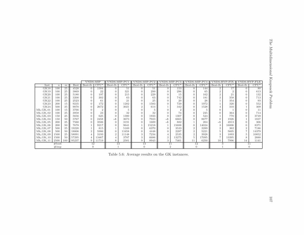
The
Multid
imen
sionalK
napsa
ckP
roblem
107
VNDS-MIP VNDS-MIP-PC1 VNDS-MIP-PC2 VNDS-MIP-PC3 VNDS-MIP-PC4 VNDS-HYP-FIX VNDS-HYP-FLEInst. n m Best Best-lb CPU* Best-lb CPU* Best-lb CPU* Best-lb CPU* Best-lb CPU* Best-lb CPU* Best-lb CPU*
GK18 100 25 4528 0 1584 0 51 0 51 0 153 0 144 2 17 0 80GK19 100 25 3869 0 22 0 321 0 299 0 296 0 65 2 2 0 613GK20 100 25 5180 0 197 0 215 0 229 0 15 0 162 2 21 0 132GK21 100 25 3200 0 302 0 63 0 63 0 742 0 181 2 358 0 713GK22 100 25 2523 0 61 0 21 0 25 0 20 0 26 1 354 0 93GK23 200 15 9235 0 172 0 1202 0 1583 0 729 0 1972 1 320 0 552GK24 500 25 9070 0 2672 0 3021 2 614 1 342 0 1528 4 310 1 309
Mk GK 01 100 15 3766 0 2 0 5 0 5 0 2 0 5 0 1 0 11Mk GK 02 100 25 3958 0 23 0 32 0 32 0 74 0 245 0 364 0 714Mk GK 03 150 25 5656 0 625 0 1380 0 1933 0 1307 0 524 1 770 0 3749Mk GK 04 150 50 5767 0 2458 -1 3673 0 7923 -1 6665 0 8677 0 1926 1 1837Mk GK 05 200 25 7560 0 3506 0 3191 0 1689 -1 882 1 204 -1 4913 0 306Mk GK 06 200 50 7678 1 9217 0 9641 1 15218 1 15688 0 14024 3 16006 0 8371Mk GK 07 500 25 19220 1 815 1 5169 0 6370 0 3533 2 3289 2 362 2 7186Mk GK 08 500 50 18806 2 5986 0 11658 0 4448 0 2287 2 5221 5 5605 7 14379Mk GK 09 1500 25 58091 4 3193 2 11148 3 7234 4 2535 2 3928 3 1893 5 10852Mk GK 10 1500 50 57295 4 13467 4 3787 3 6686 2 13275 5 17095 7 13395 8 2888Mk GK 11 2500 100 95237 9 11719 8 2581 9 8943 3 7461 11 6250 10 7996 14 1141
#best 12 13 13 11 12 3 11#imp 0 1 0 2 0 1 0
Table 5.6: Average results on the GK instances.

108 Applications of VNDS to Some Specific 0-1 MIP Problems
To complete the analysis of these results, in Table 5.7 the results obtained by VNDS-MIPand VNDS-MIP-PC3 are compared with the current best algorithms for these instances. In thistable, the values obtained by Vasquez and Hao [310] are reported in column “V&H”, whereas thevalues for LPA, IIRH and IRH are reported as in [326]. These three algorithms were validatedon the same computer, so the running time needed to reach the best solution by these methodsis also reported. The hybrid tabu search algorithm of Vasquez and Hao was executed over severaldistributed computers, and it needs several hours to obtain the best solutions. This table confirmsthe efficiency of the heuristics proposed in this section, and in particular when combining someelements of the LPA with VNDS.
LPA IIRH IRH VNDS-MIP VNDS-MIP-PC2Inst. V&H lb CPU* lb CPU* lb CPU* lb CPU* lb CPU*
GK18 4528 4528 290 4528 78 4528 680 4528 1584 4528 153GK19 3869 3869 65 3869 71 3869 25 3869 22 3869 296GK20 5180 5180 239 5180 474 5180 365 5180 197 5180 15
GK21 3200 3200 27 3200 58 3200 245 3200 302 3200 742GK22 2523 2523 60 2523 90 2523 117 2523 61 2523 20
GK23 9235 9233 5 9235 44 9235 184 9235 172 9235 729GK24 9070 9067 1 9069 1168 9070 2509 9070 2672 9069 342
Mk GK 01 3766 3766 1 3766 5 3766 1 3766 2 3766 2Mk GK 02 3958 3958 45 3958 50 3958 100 3958 23 3958 74Mk GK 03 5656 5655 457 5656 1924 5656 32 5656 625 5656 1307Mk GK 04 5767 5767 222 5767 282 5767 472 5767 2458 5768 6665Mk GK 05 7560 7560 458 7560 1261 7560 636 7560 3506 7561 882Mk GK 06 7677 7675 1727 7678 23993 7678 10042 7676 9217 7676 15688Mk GK 07 19220 19217 287 19219 8374 19219 15769 19219 815 19220 3533Mk GK 08 18806 18803 3998 18805 975 18805 11182 18804 5986 18806 2287Mk GK 09 58087 58082 396 58091 15064 58089 17732 58083 3193 58083 2535Mk GK 10 57295 57289 1999 57292 6598 57292 6355 57291 13467 57293 13275Mk GK 11 95237 95228 2260 95229 9463 95229 1921 95228 11719 95234 7461
Table 5.7: Comparison with other methods over the GK instances.
Statistical Analysis
As already mentioned in Chapter 4, the comparison between the algorithms based only on theaverages does not necessarily have to be valid. By observing only the average gap values, one canonly see that, in general, two-level decomposition methods are dominated by other VNDS-MIPbased methods. However, due to the very small differences between the gap values, it is hard tosay how significant this distinction in performance is. Also, it is difficult to single out any of thethree proposed one-level decomposition methods. This is why statistical tests have been carriedout to verify the significance of differences between the solution quality performances. Since noassumptions can be made about the distribution of the experimental results, a nonparametric(distribution-free) Friedman test [112] is applied, followed by the Nemenyi [245] post-hoc test (seeAppendix B for more details about the statistical tests), as suggested in [84].
Let I denote the set of problem instances and A the set of algorithms. The Friedman testis carried out over the entire set of |I| = 108 instances (90 instances from the OR library and18 Glover & Kochenberger instances). Averages over solution quality ranks are provided in Table5.8. According to the average ranks, VNDS-HYP-FIX has the worst performance with rank 4.74,followed by the VNDS-HYP-FLE with rank 3.46, whereas all other methods are very similar, withVNDS-MIP-PC3 being the best among the others. The value of the FF statistic for |A| = 5algorithms and |I| = 108 instances is 103.16, which is greater than the critical value 4.71 of theF -distribution with (|A| − 1, (|A| − 1)(|I| − 1)) = (4, 428) degrees of freedom at the probabilitylevel 0.001. Thus, we can conclude that there is a significant difference between the performances
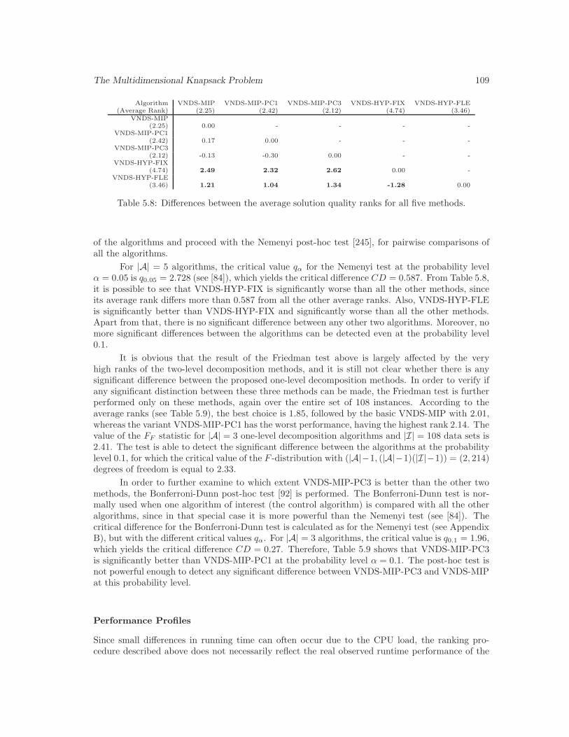
The Multidimensional Knapsack Problem 109
Algorithm VNDS-MIP VNDS-MIP-PC1 VNDS-MIP-PC3 VNDS-HYP-FIX VNDS-HYP-FLE(Average Rank) (2.25) (2.42) (2.12) (4.74) (3.46)
VNDS-MIP(2.25) 0.00 - - - -
VNDS-MIP-PC1(2.42) 0.17 0.00 - - -
VNDS-MIP-PC3(2.12) -0.13 -0.30 0.00 - -
VNDS-HYP-FIX(4.74) 2.49 2.32 2.62 0.00 -
VNDS-HYP-FLE(3.46) 1.21 1.04 1.34 -1.28 0.00
Table 5.8: Differences between the average solution quality ranks for all five methods.
of the algorithms and proceed with the Nemenyi post-hoc test [245], for pairwise comparisons ofall the algorithms.
For |A| = 5 algorithms, the critical value qα for the Nemenyi test at the probability levelα = 0.05 is q0.05 = 2.728 (see [84]), which yields the critical difference CD = 0.587. From Table 5.8,it is possible to see that VNDS-HYP-FIX is significantly worse than all the other methods, sinceits average rank differs more than 0.587 from all the other average ranks. Also, VNDS-HYP-FLEis significantly better than VNDS-HYP-FIX and significantly worse than all the other methods.Apart from that, there is no significant difference between any other two algorithms. Moreover, nomore significant differences between the algorithms can be detected even at the probability level0.1.
It is obvious that the result of the Friedman test above is largely affected by the veryhigh ranks of the two-level decomposition methods, and it is still not clear whether there is anysignificant difference between the proposed one-level decomposition methods. In order to verify ifany significant distinction between these three methods can be made, the Friedman test is furtherperformed only on these methods, again over the entire set of 108 instances. According to theaverage ranks (see Table 5.9), the best choice is 1.85, followed by the basic VNDS-MIP with 2.01,whereas the variant VNDS-MIP-PC1 has the worst performance, having the highest rank 2.14. Thevalue of the FF statistic for |A| = 3 one-level decomposition algorithms and |I| = 108 data sets is2.41. The test is able to detect the significant difference between the algorithms at the probabilitylevel 0.1, for which the critical value of the F -distribution with (|A|−1, (|A|−1)(|I|−1)) = (2, 214)degrees of freedom is equal to 2.33.
In order to further examine to which extent VNDS-MIP-PC3 is better than the other twomethods, the Bonferroni-Dunn post-hoc test [92] is performed. The Bonferroni-Dunn test is nor-mally used when one algorithm of interest (the control algorithm) is compared with all the otheralgorithms, since in that special case it is more powerful than the Nemenyi test (see [84]). Thecritical difference for the Bonferroni-Dunn test is calculated as for the Nemenyi test (see AppendixB), but with the different critical values qα. For |A| = 3 algorithms, the critical value is q0.1 = 1.96,which yields the critical difference CD = 0.27. Therefore, Table 5.9 shows that VNDS-MIP-PC3is significantly better than VNDS-MIP-PC1 at the probability level α = 0.1. The post-hoc test isnot powerful enough to detect any significant difference between VNDS-MIP-PC3 and VNDS-MIPat this probability level.
Performance Profiles
Since small differences in running time can often occur due to the CPU load, the ranking pro-cedure described above does not necessarily reflect the real observed runtime performance of the
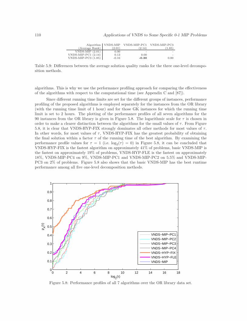
110 Applications of VNDS to Some Specific 0-1 MIP Problems
Algorithm VNDS-MIP VNDS-MIP-PC1 VNDS-MIP-PC3(Average Rank) (2.01) (2.14) (1.85)
VNDS-MIP (2.01) 0.00 - -VNDS-MIP-PC1 (2.14) 0.13 0.00 -VNDS-MIP-PC3 (1.85) -0.16 -0.30 0.00
Table 5.9: Differences between the average solution quality ranks for the three one-level decompo-sition methods.
algorithms. This is why we use the performance profiling approach for comparing the effectivenessof the algorithms with respect to the computational time (see Appendix C and [87]).
Since different running time limits are set for the different groups of instances, performanceprofiling of the proposed algorithms is employed separately for the instances from the OR library(with the running time limit of 1 hour) and for those GK instances for which the running timelimit is set to 2 hours. The plotting of the performance profiles of all seven algorithms for the90 instances from the OR library is given in Figure 5.8. The logarithmic scale for τ is chosen inorder to make a clearer distinction between the algorithms for the small values of τ . From Figure5.8, it is clear that VNDS-HYP-FIX strongly dominates all other methods for most values of τ .In other words, for most values of τ , VNDS-HYP-FIX has the greatest probability of obtainingthe final solution within a factor τ of the running time of the best algorithm. By examining theperformance profile values for τ = 1 (i.e. log2(τ) = 0) in Figure 5.8, it can be concluded thatVNDS-HYP-FIX is the fastest algorithm on approximately 41% of problems, basic VNDS-MIP isthe fastest on approximately 19% of problems, VNDS-HYP-FLE is the fastest on approximately18%, VNDS-MIP-PC4 on 9%, VNDS-MIP-PC1 and VNDS-MIP-PC2 on 5.5% and VNDS-MIP-PC3 on 2% of problems. Figure 5.8 also shows that the basic VNDS-MIP has the best runtimeperformance among all five one-level decomposition methods.
0 2 4 6 8 10 12 14 16 180
0.1
0.2
0.3
0.4
0.5
0.6
0.7
0.8
0.9
1
log2(τ)
ρ A(τ
)
VNDS−MIP−PC1VNDS−MIP−PC2VNDS−MIP−PC3VNDS−MIP−PC4VNDS−HYP−FIXVNDS−HYP−FLEVNDS−MIP
Figure 5.8: Performance profiles of all 7 algorithms over the OR library data set.
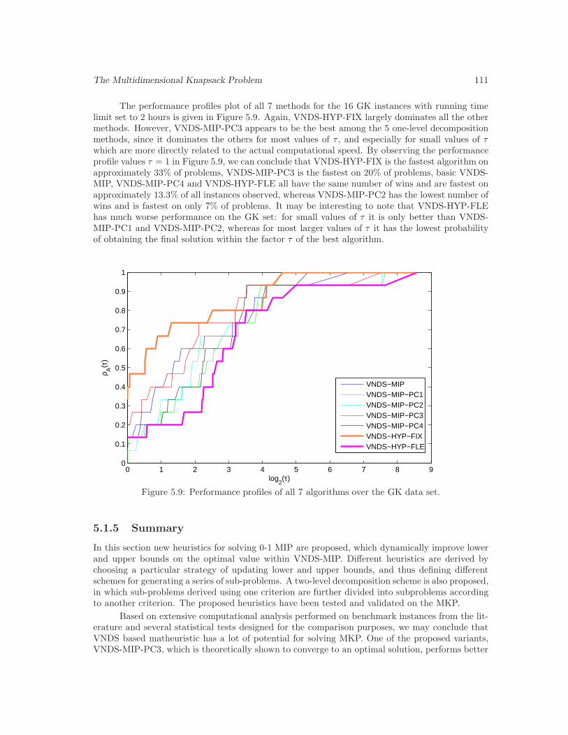
The Multidimensional Knapsack Problem 111
The performance profiles plot of all 7 methods for the 16 GK instances with running timelimit set to 2 hours is given in Figure 5.9. Again, VNDS-HYP-FIX largely dominates all the othermethods. However, VNDS-MIP-PC3 appears to be the best among the 5 one-level decompositionmethods, since it dominates the others for most values of τ , and especially for small values of τwhich are more directly related to the actual computational speed. By observing the performanceprofile values τ = 1 in Figure 5.9, we can conclude that VNDS-HYP-FIX is the fastest algorithm onapproximately 33% of problems, VNDS-MIP-PC3 is the fastest on 20% of problems, basic VNDS-MIP, VNDS-MIP-PC4 and VNDS-HYP-FLE all have the same number of wins and are fastest onapproximately 13.3% of all instances observed, whereas VNDS-MIP-PC2 has the lowest number ofwins and is fastest on only 7% of problems. It may be interesting to note that VNDS-HYP-FLEhas much worse performance on the GK set: for small values of τ it is only better than VNDS-MIP-PC1 and VNDS-MIP-PC2, whereas for most larger values of τ it has the lowest probabilityof obtaining the final solution within the factor τ of the best algorithm.
0 1 2 3 4 5 6 7 8 90
0.1
0.2
0.3
0.4
0.5
0.6
0.7
0.8
0.9
1
log2(τ)
ρ A(τ
)
VNDS−MIPVNDS−MIP−PC1VNDS−MIP−PC2VNDS−MIP−PC3VNDS−MIP−PC4VNDS−HYP−FIXVNDS−HYP−FLE
Figure 5.9: Performance profiles of all 7 algorithms over the GK data set.
5.1.5 Summary
In this section new heuristics for solving 0-1 MIP are proposed, which dynamically improve lowerand upper bounds on the optimal value within VNDS-MIP. Different heuristics are derived bychoosing a particular strategy of updating lower and upper bounds, and thus defining differentschemes for generating a series of sub-problems. A two-level decomposition scheme is also proposed,in which sub-problems derived using one criterion are further divided into subproblems accordingto another criterion. The proposed heuristics have been tested and validated on the MKP.
Based on extensive computational analysis performed on benchmark instances from the lit-erature and several statistical tests designed for the comparison purposes, we may conclude thatVNDS based matheuristic has a lot of potential for solving MKP. One of the proposed variants,VNDS-MIP-PC3, which is theoretically shown to converge to an optimal solution, performs better
112 Applications of VNDS to Some Specific 0-1 MIP Problems
than others in terms of solution quality. Furthermore, the proposed two-level decomposition meth-ods are clearly the fastest in solving very large test instances, although not as effective as othersin terms of solution quality. In fact VNDS-HYP-FIX, which is also proven to be convergent, issignificantly faster than all the other methods. In summary, the results obtained show that thisapproach is efficient and effective:
• the proposed algorithms are comparable with the state-of-the-art heuristics,
• a few new best lower bound values are obtained.
• two of the proposed methods converge to an optimal solution if no limitations regarding theexecution time or the number of iterations are imposed.
5.2 The Barge Container Ship Routing Problem
This section addresses the issue of barge container transport routes, connected to maritime con-tainer services. It means that this transport mode is considered as a hinterland transportationsystem. More precisely, we investigate the hinterland barge transport of containers arrived to ordeparting from a transshipment port (the sea port located at river mouth) by sea or mainlinecontainer ships. This clearly indicates that container barge transport acts, in this way, as a typicalfeeder service.
Determining transport routes of barge container ships has recently received a lot of attention[63, 197, 270]. One of the most important parts of this problem is adjusting the barge and seacontainer ships arrival times in the transshipment port. Optimality may be defined in accordancewith various factors (total number of transported containers, satisfaction of customer demands,shipping company profit, etc.) [6, 273, 274, 295]. Obtaining an optimal solution by any factor isvery important for doing successful transport business. Unfortunately, like in many other practicalcases, the complexity of real life problems exceeds the capacity of the present computation systems.
In this section, alternative ways for solving this problem are discussed. The use of MIPsolution heuristic methods is proposed to obtain good suboptimal solutions. Three state-of-the-artheuristics for 0-1 MIP problem are applied: local branching (LB) [104], variable neighbourhoodbranching (VNB) [169] and variable neighbourhood decomposition search for 0-1 MIP problems(VNDS-MIP) [207].
The rest of this section is organised as follows. In Subsection 5.2.1 we describe the consideredproblem: optimisation of transport routes of barge container ships. An intuitive description as wellas the mathematical formulation is given and the problem complexity is discussed. Experimentalevaluations are described in Subsection 5.2.2, while Subsection 5.2.3 contains concluding remarks.
5.2.1 Formulation of the Problem
The barge container ship routing problem addressed in this section corresponds to the problemof maximising the shipping company profit while picking up and delivering containers along theinland waterway. This form of problem was first studied in [220, 221]. The following assumptionsimpose the restrictions on the routing:
• the model assumes a weekly known cargo demand for all port pairs (origin–destination);this assumption is valid as the data regarding throughput from previous periods and futureprediction allow obtaining reliable values of these demands;

The Barge Container Ship Routing Problem 113
• the barge shipping company has to deal with transshipment costs, port dues and emptycontainer repositioning costs, in addition to the cost of container transport;
• maximum allowed route time, including sailing time and service time in ports, has to be set inaccordance with the schedule of the mainline sea container ship calling at the transshipmentport;
• the ship follows the same route during a pre-specified planning time horizon; as a commonassumption, it may be assumed that this horizon is one year long;
• the demand for empty containers at a port is the difference between the total traffic originat-ing from the port and the total loaded container traffic arriving at the port for the specifiedtime period; the assumption is valid since this study addresses the problem of determiningthe optimal route of a barge container ship for only one ship operator (similar to the casestudied by [295]);
• empty container transport [69, 82, 202] does not occur additional costs as it is performedusing the excess capacity of barge company ships (this transport actually incurs some costs,but its value is negligible in comparison with empty container handling, storage and leasingcosts);
• if a sufficient container quantity is not available at a port, the shortage is made up by leasingcontainers with the assumption that there are enough containers to be leased (for details see[295]).
Problem Overview
Routing is a fairly common problem in transport, but the barge container transport problemaddressed here has certain intrinsic features that make the design of transport routes and corre-sponding models particularly difficult:
• the barge shipping company (or charterer) wants to hire a ship or tow for a period of oneor several years (’period time charter’) in order to establish container service on a certaininland waterway;
• all the container traffic emanating from a port may not be selected for transport even if thatport is included in the route;
• the trade route is characterised by one sea or hub port located at a river mouth and severalintermediate calling river ports;
• the barge container ship route corresponds to a feeder container service; the starting andending point on the route should be the same, i.e. in this case it is the sea port wheretransshipment of containers from barge to sea container ships and vice versa takes place;
• the barge container ship travels upstream from the starting sea port to the final port locatedon the inland waterway, where from the ship sails in the downstream direction to the samesea port ending the route;
• it is not necessary for the barge container ship to visit all ports on the inland waterway; insome cases, calling at a particular port or loading all containers available at that port maynot be profitable;
• the ship doesn’t have to visit the same ports in upstream and downstream directions.

114 Applications of VNDS to Some Specific 0-1 MIP Problems
Upstreamnavigation
Downstream navigation
23
4
5
6
7
1
Figure 5.10: Example itinerary of a barge container ship
An example itinerary of a barge container ship is given in Fig. 5.10. Port 1 is the sea orhub port, while ports 2–7 represent river ports. The number associated to each port depends onits distance from port 1. The arrows indicate streams for the sequence of calling ports.
The objective when designing the transport route of a barge container ship is to maximisethe shipping company profit, i.e. the difference between the revenue arising from the service ofloaded containers (R) and the transport costs (costs related to shipping, TC and empty containerrelated costs, EC). Therefore, the objective function has the form (see [295]):
(5.4) Y = R− TC − EC.
It is necessary to generate results relating with the assumption that one ship or tow isperforming all weekly realised transport. Total number of ships employed on the route might bedetermined as the ratio of barge container ship round-trip time and service frequency of mainlinesea container ships. This model can be extended to a multi-ship problem in a straightforwardway. It meets customer demands more closely, but requires modification of the presented one-shipproblem. On the other hand, if the shipping company has an option to charter one among severalships at its disposal, then each ship can be evaluated separately using this model to determine thebest option.
Mathematical Formulation
In this section the barge container ship routing, with an aim to maximise the shipping companyprofit, is formulated as a mixed integer programming (MIP) problem. The problem is characterisedby the following input data (measurement units are given in square brackets when applied):
The Barge Container Ship Routing Problem 115
n: number of ports on the inland waterway,including the sea port;
v1 and v2: upstream and downstream bargecontainer ship speed, respectively, [km/h];
scf and scl: specific fuel and lubricant consumption,respectively [t/kWh];
fp and lp: fuel and lubricant price, respectively [US$/t];Pout: engine output (propulsion) [kW];dcc: daily time charter cost of barge container
ship [US$/day];C: carrying capacity of the barge container ship
in Twenty feet Equivalent Units [TEU];maxtt and mintt: maximum and minimum turnaround time
on a route [days];tl: total locking time at all locks between ports
1 and n [h];tb: total time of border crossings at all borders between
ports 1 and n [h];zrij : weekly expected number of loaded containers available
to be transported between ports i and j [TEU];rij : freight rate per container from port i to port j
[US$/TEU];l: distance between ending ports 1 and n [km];
ufci and lfci: unloading and loading cost, respectively perloaded container at port i [US$/TEU];
ueci and leci: unloading and loading cost, respectively perempty container at port i [US$/TEU];
peci: entry cost per call at port i [$];ufti and lfti: average unloading and loading time,
respectively, per loaded container at port i [h/TEU];ueti and leti: average unloading and loading time,
respectively, per empty container at port i [h/TEU];
pati and pdti: standby time for arrival and departure,respectively, at port i [h];
sci: storage cost at port i [US$/TEU];lci: short-term leasing cost at port i [$/TEU];
The optimal route of the barge container ship may be identified by solving the followingmathematical model (linear program). Decision variables of the model are:
• binary variables xij defined as follows:
xij =
{1 if ports i and j are directly connected in the route,0 otherwise;
• zij and wij , integers representing the number of loaded and empty containers, respectively,transported from port i to port j [TEU].
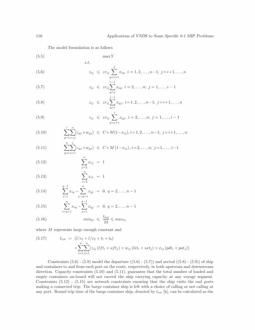
116 Applications of VNDS to Some Specific 0-1 MIP Problems
The model formulation is as follows
maxY(5.5)
s.t.
zij 6 zrij
j∑
q=i+1
xiq, i = 1, 2, . . . , n−1; j= i+1, . . . , n(5.6)
zij 6 zrij
i−1∑
q=j
xiq , i = 2, . . . , n; j = 1, . . . , i− 1(5.7)
zij 6 zrij
j−1∑
q=i
xqj , i=1, 2, . . . , n−1; j= i+1, . . . , n(5.8)
zij 6 zrij
i∑
q=j+1
xqj , i = 2, . . . , n; j = 1, . . . , i− 1(5.9)
i∑
q=1
n∑
s=j
(zqs+wqs) 6 C+M(1−xij), i=1, 2, . . . , n−1; j= i+1, . . . , n(5.10)
n∑
q=i
j∑
s=1
(zqs+wqs) 6 C+M (1−xij) , i=2, . . . , n; j=1, . . . , i−1(5.11)
n∑
j=2
x1j = 1(5.12)
n∑
i=2
xi1 = 1(5.13)
q−1∑
i=1
xiq −n∑
j=q+1
xqj = 0, q = 2, . . . , n− 1(5.14)
n∑
i=q+1
xiq −
q−1∑
j=1
xqj = 0, q = 2, . . . , n− 1(5.15)
mintt 6 ttot
246 maxtt(5.16)
where M represents large enough constant and
ttot = (l/v1 + l/v2 + tl + tb)(5.17)
+
n∑
i=1
n∑
j=1
(zij (lfti + uftj) + wij (leti + uetj) + xij (pdti + patj))
Constraints (5.6) - (5.9) model the departure ((5.6) - (5.7)) and arrival ((5.8) - (5.9)) of shipand containers to and from each port on the route, respectively, in both upstream and downstreamdirection. Capacity constraints (5.10) and (5.11), guarantee that the total number of loaded andempty containers on-board will not exceed the ship carrying capacity at any voyage segment.Constraints (5.12) - (5.15) are network constraints ensuring that the ship visits the end portsmaking a connected trip. The barge container ship is left with a choice of calling or not calling atany port. Round trip time of the barge container ship, denoted by ttot [h], can be calculated as the
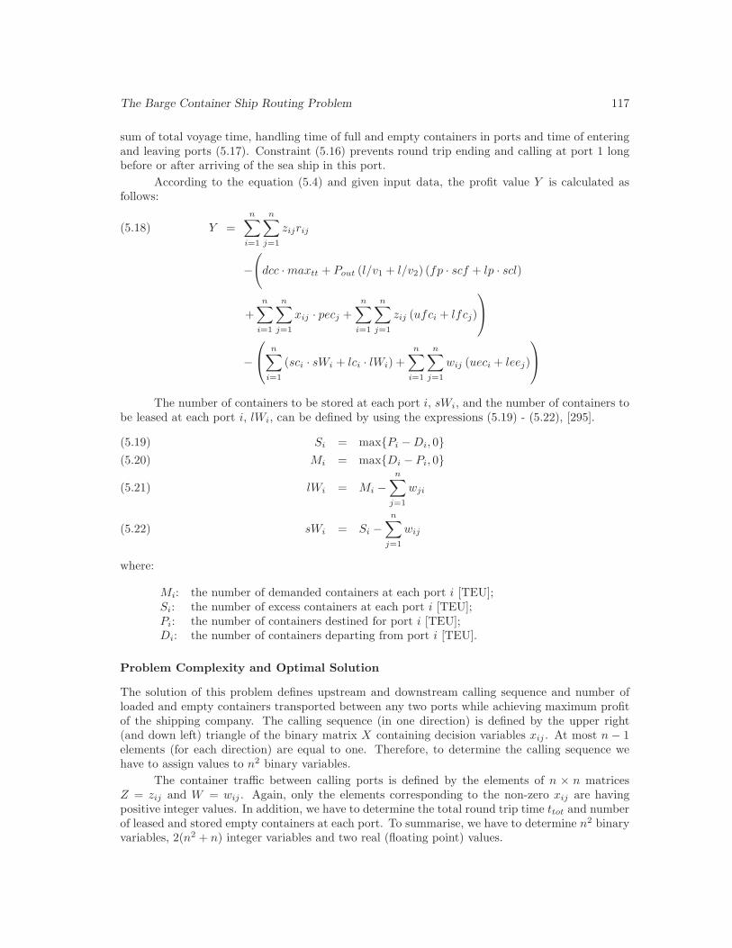
The Barge Container Ship Routing Problem 117
sum of total voyage time, handling time of full and empty containers in ports and time of enteringand leaving ports (5.17). Constraint (5.16) prevents round trip ending and calling at port 1 longbefore or after arriving of the sea ship in this port.
According to the equation (5.4) and given input data, the profit value Y is calculated asfollows:
Y =
n∑
i=1
n∑
j=1
zijrij(5.18)
−
(dcc ·maxtt + Pout (l/v1 + l/v2) (fp · scf + lp · scl)
+n∑
i=1
n∑
j=1
xij · pecj +n∑
i=1
n∑
j=1
zij (ufci + lfcj)
−
n∑
i=1
(sci · sWi + lci · lWi) +n∑
i=1
n∑
j=1
wij (ueci + leej)
The number of containers to be stored at each port i, sWi, and the number of containers tobe leased at each port i, lWi, can be defined by using the expressions (5.19) - (5.22), [295].
Si = max{Pi −Di, 0}(5.19)
Mi = max{Di − Pi, 0}(5.20)
lWi = Mi −n∑
j=1
wji(5.21)
sWi = Si −n∑
j=1
wij(5.22)
where:
Mi: the number of demanded containers at each port i [TEU];Si: the number of excess containers at each port i [TEU];Pi: the number of containers destined for port i [TEU];Di: the number of containers departing from port i [TEU].
Problem Complexity and Optimal Solution
The solution of this problem defines upstream and downstream calling sequence and number ofloaded and empty containers transported between any two ports while achieving maximum profitof the shipping company. The calling sequence (in one direction) is defined by the upper right(and down left) triangle of the binary matrix X containing decision variables xij . At most n − 1elements (for each direction) are equal to one. Therefore, to determine the calling sequence wehave to assign values to n2 binary variables.
The container traffic between calling ports is defined by the elements of n × n matricesZ = zij and W = wij . Again, only the elements corresponding to the non-zero xij are havingpositive integer values. In addition, we have to determine the total round trip time ttot and numberof leased and stored empty containers at each port. To summarise, we have to determine n2 binaryvariables, 2(n2 + n) integer variables and two real (floating point) values.

118 Applications of VNDS to Some Specific 0-1 MIP Problems
In his previous works [220, 221] Maras has used the Lingo programming language [289] tofind the optimal solutions for small instances of the given problem. Optimal solutions in [220, 221]have been obtained for 7 and 10 possibly calling ports, respectively. Switching to CPLEX ([184])and a more powerful computer under Linux, we were able to optimally solve instances with 15 portswithin 10min to 1h of CPU time, and also some of the instances with 20 ports, but the requiredCPU time exceeded 29h. Obviously, like in many other combinatorial optimisation problems, realexamples are too complex to be solved to optimality. Since the large instances cause the memorylack problems for the CPLEX MIP solver, we turn to heuristic approach in order to tackle thebarge container ship routing problem.
5.2.2 Computational Results
In this section, computational results are presented and discussed in an effort to assess and analyzethe efficiency of the presented model. We study the performance of different solution methods forour model from two points of view: mathematical programming and transportation usefulness.
Hardware and software. The applied MIP-based heuristics are all coded in the C++ program-ming language for Linux operating system and compiled with gcc (version 4.1.2) and the option-O2. The tests are performed on Intel Core 2 Duo CPU E6750 on 2.66GHz with RAM=8Gb underLinux Slackware 12, Kernel: 2.6.21.5. For exact solving we used CPLEX 11.2 ([184]) and AMPL([108, 185]) running on the same machine. Moreover, CPLEX 11.2 is used as generic MIP solverin all tested MIP-based heuristics.
Test bed. Test examples were generated randomly, in such a way that the number of ports n isvaried from 10 to 25 with increment 5. Moreover, for each value of n, 5 instances were producedwith different ship characteristics (capacities, charter costs, speed, fuel and lubricant consump-tion). In such a way we produced hard and easy examples within each problem size. The set ofinstances with their basic properties is summarised in Table 5.10.
Instance Number of variables Number ofTotal Binary General integer constraints
10ports 1 – 10ports 5 358 110 240 39815ports 1 – 15ports 5 758 240 510 81820ports 1 – 20ports 5 1308 420 880 138825ports 1 – 25ports 5 2008 650 1350 2108
Table 5.10: The barge container ship routing test bed.
Methods compared. Three state-of-the-art heuristics for 0-1 MIP problem are applied: localbranching (LB) [104], variable neighbourhood branching (VNB) [169] and variable neighbourhooddecomposition search for 0-1 MIP problems (VNDS-MIP) [207] (for more details on LB and VNBsee Chapter 2; for more details on VNDS-MIP see Chapter 4). All heuristics are compared withthe exact CPLEX 11.2 solver. After preliminary testing, it was decided to use the VNDS-MIP-PC1version of VNDS (see Section 5.1).
Parameters. According to our preliminary experiments, we have decided to use different param-eter settings for different instance sizes. Thus, different parameter settings were used for the fourgroups of instances generated for 10, 15, 20 and 25 ports, respectively. According to the preliminary
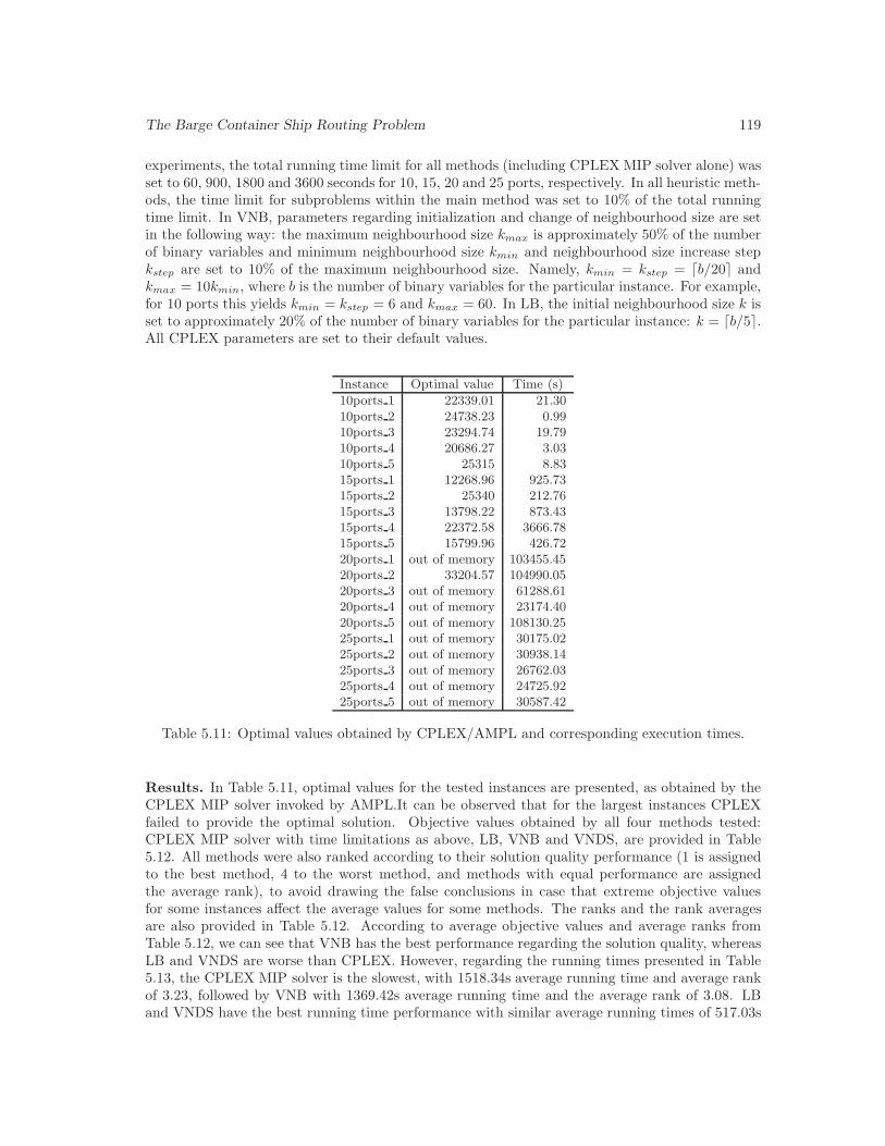
The Barge Container Ship Routing Problem 119
experiments, the total running time limit for all methods (including CPLEX MIP solver alone) wasset to 60, 900, 1800 and 3600 seconds for 10, 15, 20 and 25 ports, respectively. In all heuristic meth-ods, the time limit for subproblems within the main method was set to 10% of the total runningtime limit. In VNB, parameters regarding initialization and change of neighbourhood size are setin the following way: the maximum neighbourhood size kmax is approximately 50% of the numberof binary variables and minimum neighbourhood size kmin and neighbourhood size increase stepkstep are set to 10% of the maximum neighbourhood size. Namely, kmin = kstep = ⌈b/20⌉ andkmax = 10kmin, where b is the number of binary variables for the particular instance. For example,for 10 ports this yields kmin = kstep = 6 and kmax = 60. In LB, the initial neighbourhood size k isset to approximately 20% of the number of binary variables for the particular instance: k = ⌈b/5⌉.All CPLEX parameters are set to their default values.
Instance Optimal value Time (s)
10ports 1 22339.01 21.3010ports 2 24738.23 0.9910ports 3 23294.74 19.7910ports 4 20686.27 3.0310ports 5 25315 8.8315ports 1 12268.96 925.7315ports 2 25340 212.7615ports 3 13798.22 873.4315ports 4 22372.58 3666.7815ports 5 15799.96 426.7220ports 1 out of memory 103455.4520ports 2 33204.57 104990.0520ports 3 out of memory 61288.6120ports 4 out of memory 23174.4020ports 5 out of memory 108130.2525ports 1 out of memory 30175.0225ports 2 out of memory 30938.1425ports 3 out of memory 26762.0325ports 4 out of memory 24725.9225ports 5 out of memory 30587.42
Table 5.11: Optimal values obtained by CPLEX/AMPL and corresponding execution times.
Results. In Table 5.11, optimal values for the tested instances are presented, as obtained by theCPLEX MIP solver invoked by AMPL.It can be observed that for the largest instances CPLEXfailed to provide the optimal solution. Objective values obtained by all four methods tested:CPLEX MIP solver with time limitations as above, LB, VNB and VNDS, are provided in Table5.12. All methods were also ranked according to their solution quality performance (1 is assignedto the best method, 4 to the worst method, and methods with equal performance are assignedthe average rank), to avoid drawing the false conclusions in case that extreme objective valuesfor some instances affect the average values for some methods. The ranks and the rank averagesare also provided in Table 5.12. According to average objective values and average ranks fromTable 5.12, we can see that VNB has the best performance regarding the solution quality, whereasLB and VNDS are worse than CPLEX. However, regarding the running times presented in Table5.13, the CPLEX MIP solver is the slowest, with 1518.34s average running time and average rankof 3.23, followed by VNB with 1369.42s average running time and the average rank of 3.08. LBand VNDS have the best running time performance with similar average running times of 517.03s
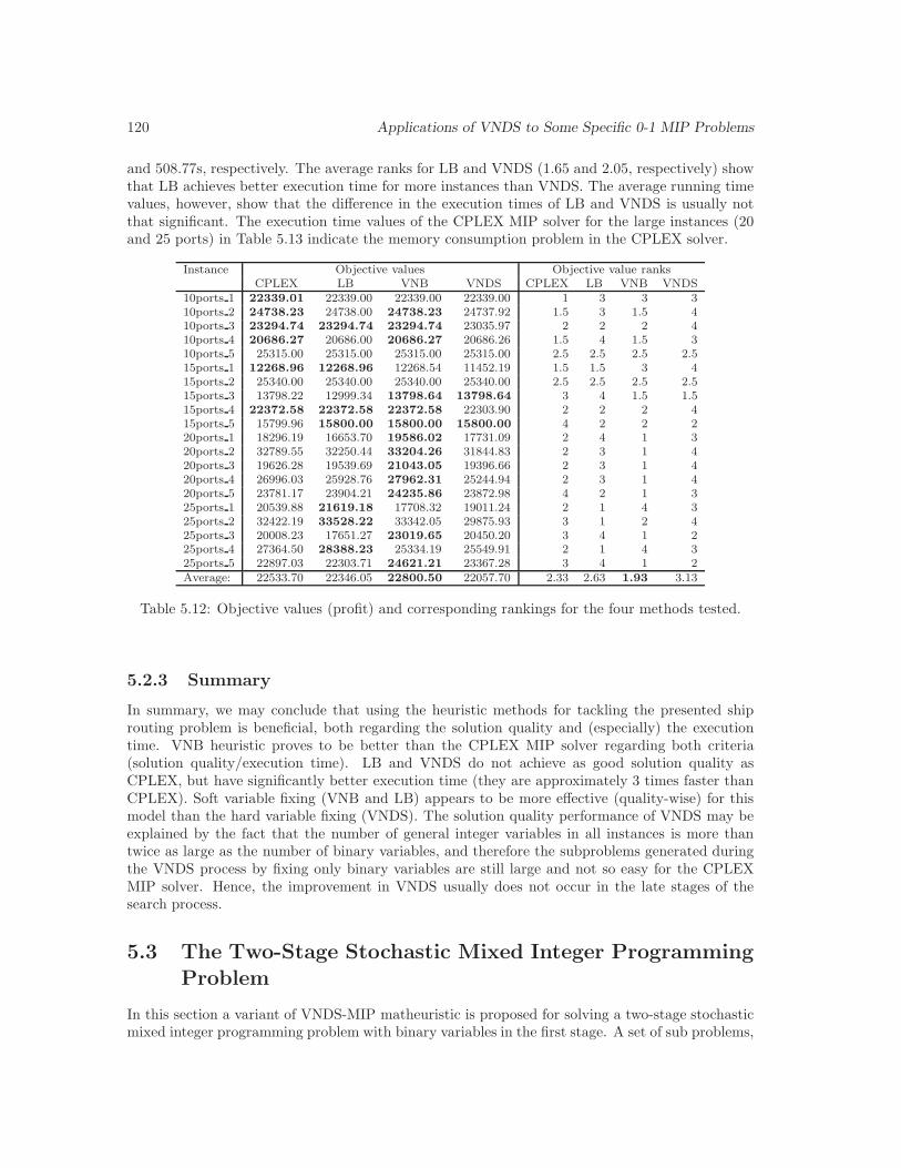
120 Applications of VNDS to Some Specific 0-1 MIP Problems
and 508.77s, respectively. The average ranks for LB and VNDS (1.65 and 2.05, respectively) showthat LB achieves better execution time for more instances than VNDS. The average running timevalues, however, show that the difference in the execution times of LB and VNDS is usually notthat significant. The execution time values of the CPLEX MIP solver for the large instances (20and 25 ports) in Table 5.13 indicate the memory consumption problem in the CPLEX solver.
Instance Objective values Objective value ranksCPLEX LB VNB VNDS CPLEX LB VNB VNDS
10ports 1 22339.01 22339.00 22339.00 22339.00 1 3 3 310ports 2 24738.23 24738.00 24738.23 24737.92 1.5 3 1.5 410ports 3 23294.74 23294.74 23294.74 23035.97 2 2 2 410ports 4 20686.27 20686.00 20686.27 20686.26 1.5 4 1.5 310ports 5 25315.00 25315.00 25315.00 25315.00 2.5 2.5 2.5 2.515ports 1 12268.96 12268.96 12268.54 11452.19 1.5 1.5 3 415ports 2 25340.00 25340.00 25340.00 25340.00 2.5 2.5 2.5 2.515ports 3 13798.22 12999.34 13798.64 13798.64 3 4 1.5 1.515ports 4 22372.58 22372.58 22372.58 22303.90 2 2 2 415ports 5 15799.96 15800.00 15800.00 15800.00 4 2 2 220ports 1 18296.19 16653.70 19586.02 17731.09 2 4 1 320ports 2 32789.55 32250.44 33204.26 31844.83 2 3 1 420ports 3 19626.28 19539.69 21043.05 19396.66 2 3 1 420ports 4 26996.03 25928.76 27962.31 25244.94 2 3 1 420ports 5 23781.17 23904.21 24235.86 23872.98 4 2 1 325ports 1 20539.88 21619.18 17708.32 19011.24 2 1 4 325ports 2 32422.19 33528.22 33342.05 29875.93 3 1 2 425ports 3 20008.23 17651.27 23019.65 20450.20 3 4 1 225ports 4 27364.50 28388.23 25334.19 25549.91 2 1 4 325ports 5 22897.03 22303.71 24621.21 23367.28 3 4 1 2Average: 22533.70 22346.05 22800.50 22057.70 2.33 2.63 1.93 3.13
Table 5.12: Objective values (profit) and corresponding rankings for the four methods tested.
5.2.3 Summary
In summary, we may conclude that using the heuristic methods for tackling the presented shiprouting problem is beneficial, both regarding the solution quality and (especially) the executiontime. VNB heuristic proves to be better than the CPLEX MIP solver regarding both criteria(solution quality/execution time). LB and VNDS do not achieve as good solution quality asCPLEX, but have significantly better execution time (they are approximately 3 times faster thanCPLEX). Soft variable fixing (VNB and LB) appears to be more effective (quality-wise) for thismodel than the hard variable fixing (VNDS). The solution quality performance of VNDS may beexplained by the fact that the number of general integer variables in all instances is more thantwice as large as the number of binary variables, and therefore the subproblems generated duringthe VNDS process by fixing only binary variables are still large and not so easy for the CPLEXMIP solver. Hence, the improvement in VNDS usually does not occur in the late stages of thesearch process.
5.3 The Two-Stage Stochastic Mixed Integer ProgrammingProblem
In this section a variant of VNDS-MIP matheuristic is proposed for solving a two-stage stochasticmixed integer programming problem with binary variables in the first stage. A set of sub problems,
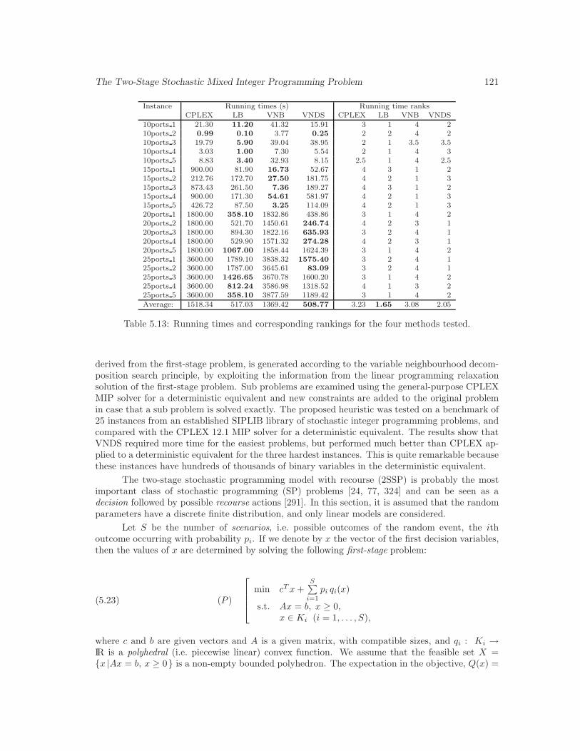
The Two-Stage Stochastic Mixed Integer Programming Problem 121
Instance Running times (s) Running time ranksCPLEX LB VNB VNDS CPLEX LB VNB VNDS
10ports 1 21.30 11.20 41.32 15.91 3 1 4 210ports 2 0.99 0.10 3.77 0.25 2 2 4 210ports 3 19.79 5.90 39.04 38.95 2 1 3.5 3.510ports 4 3.03 1.00 7.30 5.54 2 1 4 310ports 5 8.83 3.40 32.93 8.15 2.5 1 4 2.515ports 1 900.00 81.90 16.73 52.67 4 3 1 215ports 2 212.76 172.70 27.50 181.75 4 2 1 315ports 3 873.43 261.50 7.36 189.27 4 3 1 215ports 4 900.00 171.30 54.61 581.97 4 2 1 315ports 5 426.72 87.50 3.25 114.09 4 2 1 320ports 1 1800.00 358.10 1832.86 438.86 3 1 4 220ports 2 1800.00 521.70 1450.61 246.74 4 2 3 120ports 3 1800.00 894.30 1822.16 635.93 3 2 4 120ports 4 1800.00 529.90 1571.32 274.28 4 2 3 120ports 5 1800.00 1067.00 1858.44 1624.39 3 1 4 225ports 1 3600.00 1789.10 3838.32 1575.40 3 2 4 125ports 2 3600.00 1787.00 3645.61 83.09 3 2 4 125ports 3 3600.00 1426.65 3670.78 1600.20 3 1 4 225ports 4 3600.00 812.24 3586.98 1318.52 4 1 3 225ports 5 3600.00 358.10 3877.59 1189.42 3 1 4 2Average: 1518.34 517.03 1369.42 508.77 3.23 1.65 3.08 2.05
Table 5.13: Running times and corresponding rankings for the four methods tested.
derived from the first-stage problem, is generated according to the variable neighbourhood decom-position search principle, by exploiting the information from the linear programming relaxationsolution of the first-stage problem. Sub problems are examined using the general-purpose CPLEXMIP solver for a deterministic equivalent and new constraints are added to the original problemin case that a sub problem is solved exactly. The proposed heuristic was tested on a benchmark of25 instances from an established SIPLIB library of stochastic integer programming problems, andcompared with the CPLEX 12.1 MIP solver for a deterministic equivalent. The results show thatVNDS required more time for the easiest problems, but performed much better than CPLEX ap-plied to a deterministic equivalent for the three hardest instances. This is quite remarkable becausethese instances have hundreds of thousands of binary variables in the deterministic equivalent.
The two-stage stochastic programming model with recourse (2SSP) is probably the mostimportant class of stochastic programming (SP) problems [24, 77, 324] and can be seen as adecision followed by possible recourse actions [291]. In this section, it is assumed that the randomparameters have a discrete finite distribution, and only linear models are considered.
Let S be the number of scenarios, i.e. possible outcomes of the random event, the ithoutcome occurring with probability pi. If we denote by x the vector of the first decision variables,then the values of x are determined by solving the following first-stage problem:
(5.23) (P )
min cT x +S∑
i=1
pi qi(x)
s.t. Ax = b, x ≥ 0,x ∈ Ki (i = 1, . . . , S),
where c and b are given vectors and A is a given matrix, with compatible sizes, and qi : Ki →IR is a polyhedral (i.e. piecewise linear) convex function. We assume that the feasible set X ={x |Ax = b, x ≥ 0} is a non-empty bounded polyhedron. The expectation in the objective, Q(x) =

122 Applications of VNDS to Some Specific 0-1 MIP Problems
S∑i=1
pi qi(x), is called the expected recourse function. This is a polyhedral convex function with the
domain K = K1 ∩ . . . ∩KS.
Once the first decision has been made with the result x and the ith scenario realised, thesecond decision concerns solving the following second-stage problem or recourse problem:
(5.24) (Ri(x))
min qi(x) = qTi y
s.t. Tix + Wiy = hi,y ≥ 0,
where qi, hi are given vectors, Ti, Wi are given matrices of compatible sizes and y denotes thedecision variable. We assume that the optimal objective value qi(x), x ∈ Ki, of the recourseproblem Ri(x) satisfies qi(x) > −∞.1
The two-stage stochastic programming problem (5.23)-(5.24) can be formulated as a singlelinear programming (LP) problem called the deterministic equivalent problem (DEP for short):
(5.25)
min cT x + p1qT1 y1 + . . . + pSqT
S yS
s.t. Ax = b,T1x + W1y1 = h1,...
. . ....
TSx + WSyS = hS ,x ≥ 0, y1 ≥ 0, . . . , yS ≥ 0.
In this section we deal with 0-1 mixed integer 2SSP models, where both the first-stage andthe second-stage problem can contain variables with integrality constraints and the set of binaryvariables in the first-stage problem is non-empty. In other words, it is assumed that the feasibleset X of the first-stage problem (5.23) is of the form
(5.26) X = {0, 1}n1 × Z+0
n2
× R+0
n3
, n1, n2, n3 ∈ Z+0 , n1 > 0,
where Z+0 = N∪{0}, R+
0 = {x ∈ R | x ≥ 0}, n1 is the number of binary variables, n2 is the numberof general integer variables and n3 is the number of continuous variables. In that case, the feasibleset X of the first-stage problem of the linear programming relaxation of the problem (5.23)-(5.24)
is given by X = [0, 1]n1 × R+0
n2+n3
.
Since the first-stage problem (5.23) is a special case of the 0-1 MIP problem, the (partial)distance (see (2.5) and (2.13)) and neighbourhood structures (see (2.3)) can be defined in thefeasible set X of (5.23) in the same way as for any 0-1 MIP problem in general. By introducingthe neighbourhood structures into the feasible set X of problem (5.23), it becomes possible toapply some variable neighbourhood search [237] based heuristic for solving the first-stage problem(5.23). In this section, the variable neighbourhood decomposition search [168] is used to tackle thefirst-stage problem (5.23) and thus speed up the overall solution process for a given 2SSP problem(5.23)-(5.24).
The rest of this section is organised as follows. In Subsection 5.3.1, we provide a briefoverview of the existing solution methods for 0-1 mixed integer 2SSP. In Subsection 5.3.2, we pro-vide a detailed description of the proposed variable neighbourhood decomposition search heuristicfor 0-1 mixed integer 2SSP. Next, in Subsection 5.3.3, we analyse the performance of the proposedmethod as compared to the commercial IBM ILOG CPLEX 12.1 MIP solver for the deterministicequivalent. In Subsection 5.3.4, we summarise our conclusions.
1Equivalently, we assume that the dual of the recourse problem Ri(x) has a feasible solution. Solvability of thedual problem does not depend on x.
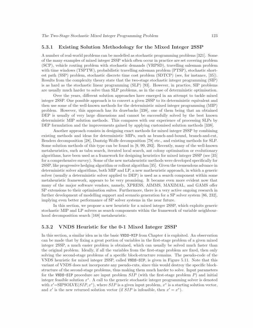
The Two-Stage Stochastic Mixed Integer Programming Problem 123
5.3.1 Existing Solution Methodology for the Mixed Integer 2SSP
A number of real-world problems can be modelled as stochastic programming problems [321]. Someof the many examples of mixed integer 2SSP which often occur in practice are set covering problem(SCP), vehicle routing problem with stochastic demands (VRPSD), travelling salesman problemwith time windows (TSPTW), probabilistic travelling salesman problem (PTSP), stochastic short-est path (SSP) problem, stochastic discrete time cost problem (SDTCP) (see, for instance, [35]).Results from the complexity theory state that the two-stage stochastic integer programming (SIP)is as hard as the stochastic linear programming (SLP) [93]. However, in practice, SIP problemsare usually much harder to solve than SLP problems, as in the case of deterministic optimisation.
Over the years, different solution approaches have emerged in an attempt to tackle mixedinteger 2SSP. One possible approach is to convert a given 2SSP to its deterministic equivalent andthen use some of the well-known methods for the deterministic mixed integer programming (MIP)problem. However, this approach has its drawbacks [338], one of them being that an obtainedDEP is usually of very large dimensions and cannot be successfully solved by the best knowndeterministic MIP solution methods. This compares with our experience of processing SLPs byDEP formulation and the improvements gained by applying customised solution methods [338].
Another approach consists in designing exact methods for mixed integer 2SSP by combiningexisting methods and ideas for deterministic MIPs, such as branch-and-bound, branch-and-cut,Benders decomposition [28], Dantzig-Wolfe decomposition [78] etc., and existing methods for SLP.Some solution methods of this type can be found in [9, 99, 292]. Recently, many of the well-knownmetaheuristics, such as tabu search, iterated local search, ant colony optimisation or evolutionaryalgorithms, have been used as a framework for designing heuristics for mixed integer 2SSP (see [35]for a comprehensive survey). Some of the new metaheuristic methods were developed specifically for2SSP, like progressive hedging algorithm or rollout algorithm [35]. Given the tremendous advance indeterministic solver algorithms, both MIP and LP, a new matheuristic approach, in which a genericsolver (usually a deterministic solver applied to DEP) is used as a search component within somemetaheuristic framework, appears to be very promising. It became even more evident now thatmany of the major software vendors, namely, XPRESS, AIMMS, MAXIMAL, and GAMS offerSP extensions to their optimisation suites. Furthermore, there is a very active ongoing research infurther development of modelling support and scenario generation for a SP solver system [86, 232],implying even better performance of SP solver systems in the near future.
In this section, we propose a new heuristic for a mixed integer 2SSP, which exploits genericstochastic MIP and LP solvers as search components within the framework of variable neighbour-hood decomposition search [168] metaheuristic.
5.3.2 VNDS Heuristic for the 0-1 Mixed Integer 2SSP
In this section, a similar idea as in the basic VNDS-MIP from Chapter 4 is exploited. An observationcan be made that by fixing a great portion of variables in the first-stage problem of a given mixedinteger 2SSP, a much easier problem is obtained, which can usually be solved much faster thanthe original problem. Ideally, if all the variables from the first-stage problem are fixed, then onlysolving the second-stage problems of a specific block-structure remains. The pseudo-code of theVNDS heuristic for mixed integer 2SSP, called VNDS-SIP, is given in Figure 5.11. Note that thisvariant of VNDS does not incorporate any pseudo-cuts, since this would destroy the specific block-structure of the second-stage problems, thus making them much harder to solve. Input parametersfor the VNDS-SIP procedure are input problem SIP (with the first-stage problem P ) and initialinteger feasible solution x∗. A call to the generic stochastic integer programming solver is denotedwith x′=SIPSOLVE(SIP, x∗), where SIP is a given input problem, x∗ is a starting solution vector,and x′ is the new returned solution vector (if SIP is infeasible, then x′ = x∗).
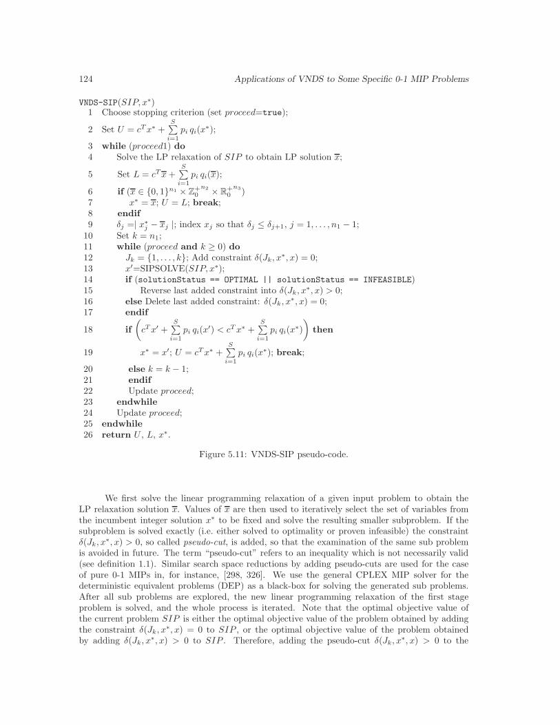
124 Applications of VNDS to Some Specific 0-1 MIP Problems
VNDS-SIP(SIP, x∗)1 Choose stopping criterion (set proceed=true);
2 Set U = cT x∗ +S∑
i=1
pi qi(x∗);
3 while (proceed1) do4 Solve the LP relaxation of SIP to obtain LP solution x;
5 Set L = cT x +S∑
i=1
pi qi(x);
6 if (x ∈ {0, 1}n1 × Z+0
n2
× R+0
n3
)7 x∗ = x; U = L; break;8 endif9 δj =| x∗j − xj |; index xj so that δj ≤ δj+1, j = 1, . . . , n1 − 1;
10 Set k = n1;11 while (proceed and k ≥ 0) do12 Jk = {1, . . . , k}; Add constraint δ(Jk, x∗, x) = 0;13 x′=SIPSOLVE(SIP, x∗);14 if (solutionStatus == OPTIMAL || solutionStatus == INFEASIBLE)15 Reverse last added constraint into δ(Jk, x∗, x) > 0;16 else Delete last added constraint: δ(Jk, x∗, x) = 0;17 endif
18 if
(cT x′ +
S∑i=1
pi qi(x′) < cT x∗ +
S∑i=1
pi qi(x∗)
)then
19 x∗ = x′; U = cT x∗ +S∑
i=1
pi qi(x∗); break;
20 else k = k − 1;21 endif22 Update proceed;23 endwhile24 Update proceed;25 endwhile26 return U , L, x∗.
Figure 5.11: VNDS-SIP pseudo-code.
We first solve the linear programming relaxation of a given input problem to obtain theLP relaxation solution x. Values of x are then used to iteratively select the set of variables fromthe incumbent integer solution x∗ to be fixed and solve the resulting smaller subproblem. If thesubproblem is solved exactly (i.e. either solved to optimality or proven infeasible) the constraintδ(Jk, x∗, x) > 0, so called pseudo-cut, is added, so that the examination of the same sub problemis avoided in future. The term “pseudo-cut” refers to an inequality which is not necessarily valid(see definition 1.1). Similar search space reductions by adding pseudo-cuts are used for the caseof pure 0-1 MIPs in, for instance, [298, 326]. We use the general CPLEX MIP solver for thedeterministic equivalent problems (DEP) as a black-box for solving the generated sub problems.After all sub problems are explored, the new linear programming relaxation of the first stageproblem is solved, and the whole process is iterated. Note that the optimal objective value ofthe current problem SIP is either the optimal objective value of the problem obtained by addingthe constraint δ(Jk, x∗, x) = 0 to SIP , or the optimal objective value of the problem obtainedby adding δ(Jk, x∗, x) > 0 to SIP . Therefore, adding the pseudo-cut δ(Jk, x∗, x) > 0 to the
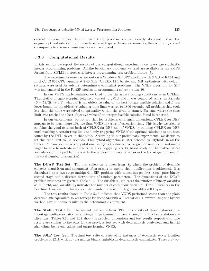
The Two-Stage Stochastic Mixed Integer Programming Problem 125
current problem, in case that the current sub problem is solved exactly, does not discard theoriginal optimal solution from the reduced search space. In our experiments, the condition proceedcorresponds to the maximum execution time allowed.
5.3.3 Computational Results
In this section we report the results of our computational experiments on two-stage stochasticinteger programming problems. All the benchmark problems we used are available in the SMPSformat from SIPLIB, a stochastic integer programming test problem library [7].
The experiments were carried out on a Windows XP SP2 machine with 3 GB of RAM andIntel Core2 660 CPU running at 2.40 GHz. CPLEX 12.1 barrier and MIP optimisers with defaultsettings were used for solving deterministic equivalent problems. The VNDS algorithm for SIPwas implemented in the FortSP stochastic programming solver system [98].
In our VNDS implementation we tried to use the same stopping conditions as in CPLEX.The relative mipgap stopping tolerance was set to 0.01% and it was computed using the formula(U − L)/(|U |+ 0.1), where U is the objective value of the best integer feasible solution and L is alower bound on the objective value. A time limit was set to 1800 seconds. All problems that tookless than this time were solved to optimality within the given tolerance. For runs where the timelimit was reached the best objective value of an integer feasible solution found is reported.
In our experiments, we noticed that for problems with small dimensions, CPLEX for DEPappears to be much more effective than VNDS in terms of execution time. This is why we tried tocombine the good features both of CPLEX for DEP and of VNDS, by running CPLEX for DEPuntil reaching a certain time limit and only triggering VNDS if the optimal solution has not beenfound by the DEP solver in that time. According to our preliminary experiments, we decide toset this time limit to 720 seconds. This hybrid algorithm is later denoted as ”Hybrid” in all thetables. A more extensive computational analysis (performed on a greater number of instances)might be able to indicate another criteria for triggering VNDS, based solely on the mathematicalformulation of the problem (probably the portion of binary variables in the first-stage problem, orthe total number of scenarios).
The DCAP Test Set. The first collection is taken from [8], where the problem of dynamiccapacity acquisition and assignment often arising in supply chain applications is addressed. It isformulated as a two-stage multiperiod SIP problem with mixed-integer first stage, pure binarysecond stage and a discrete distribution of random parameters. The dimensions of the DCAPproblem instances are given in Table 5.14. The variable n1 indicates the number of binary variablesas in (5.26), and variable n3 indicates the number of continuous variables. For all instances in thebenchmark we used in this section, the number of general integer variables is 0 (n2 = 0).
The test results shown in Table 5.15 indicate that VNDS performed worse than the plaindeterministic equivalent solver (except for decap332 with 300 scenarios). However using the hybridmethod gave the same results as the deterministic equivalent.
The SIZES Test Set. The second test set is from [190]. It consists of three instances of atwo-stage multiperiod stochastic integer programming problem arising in product substitution ap-plications. Tables 5.16 and 5.17 show the problem dimensions and test results respectively. Theresults are similar to the ones for the previous test set with deterministic equivalent and hybridalgorithms being equivalent and outperforming VNDS.
The SSLP Test Set. The final test suite consists of 12 instances of stochastic server locationproblems by [247] with up to a million binary variables in deterministic equivalents. These are two-

126 Applications of VNDS to Some Specific 0-1 MIP Problems
Stage 1 Det. Eq.
Name Scen n1 n3 Rows Columns Nonzeros Binaries
dcap233200 6 6 3006 5412 11412 5406300 6 6 4506 8112 17112 8106500 6 6 7506 13512 28512 13506
dcap243200 6 6 3606 7212 14412 7206300 6 6 5406 10812 21612 10806500 6 6 9006 18012 36012 18006
dcap332200 6 6 2406 4812 10212 4806300 6 6 3606 7212 15312 7206500 6 6 6006 12012 25512 12006
dcap342200 6 6 2806 6412 13012 6406300 6 6 4206 9612 19512 9606500 6 6 7006 16012 32512 16006
Table 5.14: Dimensions of the DCAP problems
Det. Eq. VNDS Hybrid
Name Scen Time Obj Time Obj Time Obj
dcap233200 2.25 1834.60 13.67 1834.59 1.31 1834.60300 1800.86 1644.36 1800.25 1644.36 1800.16 1644.36500 3.88 1737.52 60.38 1737.52 3.59 1737.52
dcap243200 4.22 2322.59 34.31 2322.50 4.06 2322.59300 12.03 2559.45 24.86 2559.45 11.88 2559.45500 34.64 2167.40 65.67 2167.40 34.53 2167.40
dcap332200 1800.64 1060.70 1800.15 1060.70 1800.02 1060.70300 1800.65 1252.88 1423.54 1252.88 1800.01 1252.88500 1800.70 1588.81 1800.31 1588.82 1800.05 1588.82
dcap342200 90.86 1619.59 144.74 1619.58 91.34 1619.59300 1800.62 2067.70 1800.25 2067.70 1800.02 2067.70500 1800.55 1904.66 1800.41 1904.73 1800.02 1904.66
Table 5.15: Test results for DCAP
Stage 1 Det. Eq.
Name Scen n1 n3 Rows Columns Nonzeros Binaries
SIZES3 10 65 124 300 795 405 10 65 186 450 1225 60
10 10 65 341 825 2300 110
Table 5.16: Dimensions of the SIZES problems
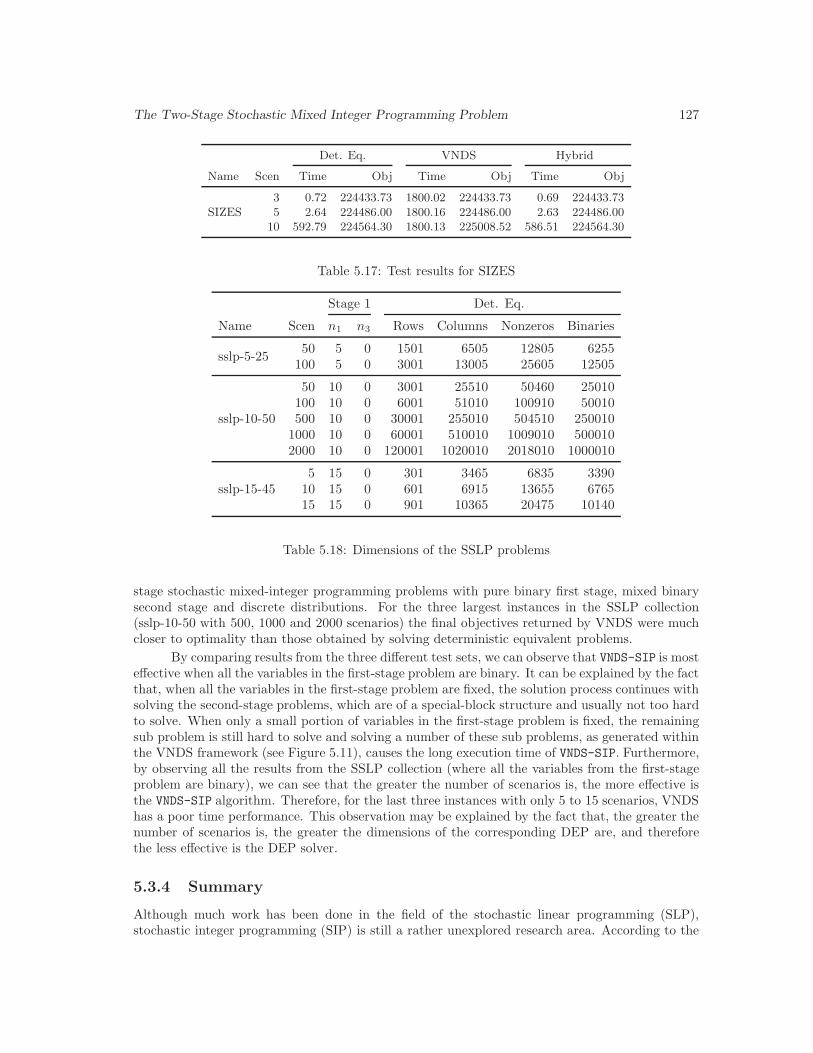
The Two-Stage Stochastic Mixed Integer Programming Problem 127
Det. Eq. VNDS Hybrid
Name Scen Time Obj Time Obj Time Obj
SIZES3 0.72 224433.73 1800.02 224433.73 0.69 224433.735 2.64 224486.00 1800.16 224486.00 2.63 224486.00
10 592.79 224564.30 1800.13 225008.52 586.51 224564.30
Table 5.17: Test results for SIZES
Stage 1 Det. Eq.
Name Scen n1 n3 Rows Columns Nonzeros Binaries
sslp-5-2550 5 0 1501 6505 12805 6255
100 5 0 3001 13005 25605 12505
sslp-10-50
50 10 0 3001 25510 50460 25010100 10 0 6001 51010 100910 50010500 10 0 30001 255010 504510 250010
1000 10 0 60001 510010 1009010 5000102000 10 0 120001 1020010 2018010 1000010
sslp-15-455 15 0 301 3465 6835 3390
10 15 0 601 6915 13655 676515 15 0 901 10365 20475 10140
Table 5.18: Dimensions of the SSLP problems
stage stochastic mixed-integer programming problems with pure binary first stage, mixed binarysecond stage and discrete distributions. For the three largest instances in the SSLP collection(sslp-10-50 with 500, 1000 and 2000 scenarios) the final objectives returned by VNDS were muchcloser to optimality than those obtained by solving deterministic equivalent problems.
By comparing results from the three different test sets, we can observe that VNDS-SIP is mosteffective when all the variables in the first-stage problem are binary. It can be explained by the factthat, when all the variables in the first-stage problem are fixed, the solution process continues withsolving the second-stage problems, which are of a special-block structure and usually not too hardto solve. When only a small portion of variables in the first-stage problem is fixed, the remainingsub problem is still hard to solve and solving a number of these sub problems, as generated withinthe VNDS framework (see Figure 5.11), causes the long execution time of VNDS-SIP. Furthermore,by observing all the results from the SSLP collection (where all the variables from the first-stageproblem are binary), we can see that the greater the number of scenarios is, the more effective isthe VNDS-SIP algorithm. Therefore, for the last three instances with only 5 to 15 scenarios, VNDShas a poor time performance. This observation may be explained by the fact that, the greater thenumber of scenarios is, the greater the dimensions of the corresponding DEP are, and thereforethe less effective is the DEP solver.
5.3.4 Summary
Although much work has been done in the field of the stochastic linear programming (SLP),stochastic integer programming (SIP) is still a rather unexplored research area. According to the
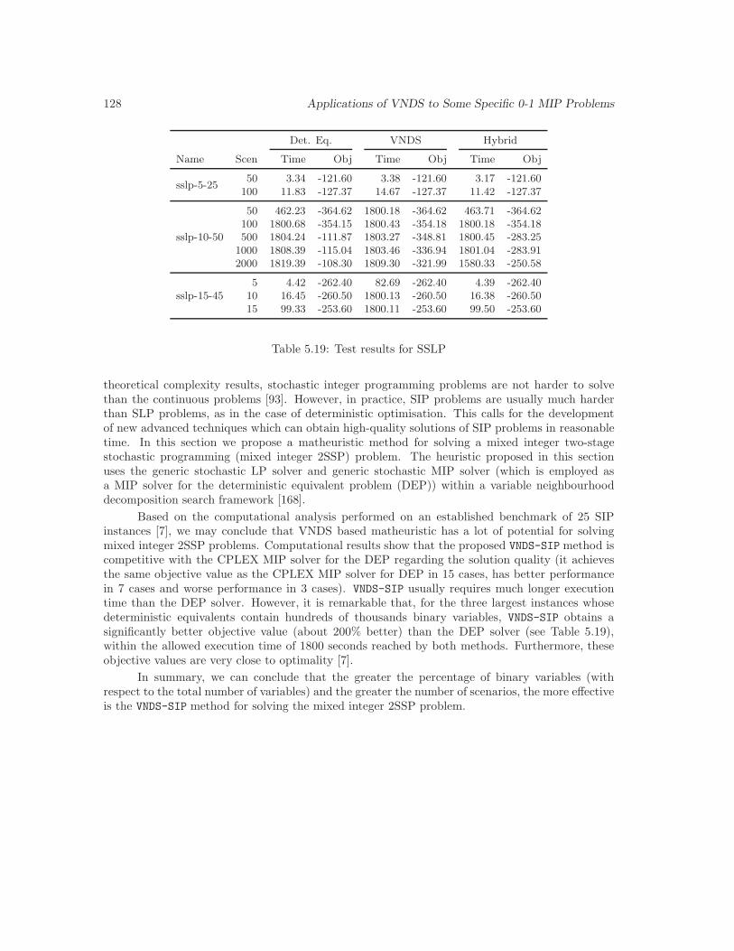
128 Applications of VNDS to Some Specific 0-1 MIP Problems
Det. Eq. VNDS Hybrid
Name Scen Time Obj Time Obj Time Obj
sslp-5-2550 3.34 -121.60 3.38 -121.60 3.17 -121.60
100 11.83 -127.37 14.67 -127.37 11.42 -127.37
sslp-10-50
50 462.23 -364.62 1800.18 -364.62 463.71 -364.62100 1800.68 -354.15 1800.43 -354.18 1800.18 -354.18500 1804.24 -111.87 1803.27 -348.81 1800.45 -283.25
1000 1808.39 -115.04 1803.46 -336.94 1801.04 -283.912000 1819.39 -108.30 1809.30 -321.99 1580.33 -250.58
sslp-15-455 4.42 -262.40 82.69 -262.40 4.39 -262.40
10 16.45 -260.50 1800.13 -260.50 16.38 -260.5015 99.33 -253.60 1800.11 -253.60 99.50 -253.60
Table 5.19: Test results for SSLP
theoretical complexity results, stochastic integer programming problems are not harder to solvethan the continuous problems [93]. However, in practice, SIP problems are usually much harderthan SLP problems, as in the case of deterministic optimisation. This calls for the developmentof new advanced techniques which can obtain high-quality solutions of SIP problems in reasonabletime. In this section we propose a matheuristic method for solving a mixed integer two-stagestochastic programming (mixed integer 2SSP) problem. The heuristic proposed in this sectionuses the generic stochastic LP solver and generic stochastic MIP solver (which is employed asa MIP solver for the deterministic equivalent problem (DEP)) within a variable neighbourhooddecomposition search framework [168].
Based on the computational analysis performed on an established benchmark of 25 SIPinstances [7], we may conclude that VNDS based matheuristic has a lot of potential for solvingmixed integer 2SSP problems. Computational results show that the proposed VNDS-SIP method iscompetitive with the CPLEX MIP solver for the DEP regarding the solution quality (it achievesthe same objective value as the CPLEX MIP solver for DEP in 15 cases, has better performancein 7 cases and worse performance in 3 cases). VNDS-SIP usually requires much longer executiontime than the DEP solver. However, it is remarkable that, for the three largest instances whosedeterministic equivalents contain hundreds of thousands binary variables, VNDS-SIP obtains asignificantly better objective value (about 200% better) than the DEP solver (see Table 5.19),within the allowed execution time of 1800 seconds reached by both methods. Furthermore, theseobjective values are very close to optimality [7].
In summary, we can conclude that the greater the percentage of binary variables (withrespect to the total number of variables) and the greater the number of scenarios, the more effectiveis the VNDS-SIP method for solving the mixed integer 2SSP problem.
Chapter 6
Variable Neighbourhood Searchand 0-1 MIP Feasibility
Various heuristic methods have been designed in an attempt to find good near-optimal solutionsof hard 0-1 MIPs. Most of them start from a given feasible solution and try to improve it.Still, finding a feasible solution of 0-1 MIP is proven to be np-complete [331] and for a numberof instances remains hard in practice. This calls for the development of efficient constructiveheuristics which can attain feasible solutions in short time. A number of heuristics which addressthe problem of MIP feasibility have been proposed in the literature, although the research inthis area has only significantly intensified in the last decade. Whereas some of the proposedheuristics are based on the standard metaheuristic frameworks, such as tabu search [213], geneticalgorithm [246], scatter search [134], the others are specific approaches intended solely for tacklingthe 0-1 MIP feasibility problem. Interior point based methods were proposed in [176]. Pivotingmethods, in which special pivot moves are constructed and performed in order to decrease theinteger infeasibility, were proposed in [19, 20, 94, 214]. Few heuristics proposed in [187] combineconstraint programming and LP relaxations in order to locate feasible solutions by means of thespecialised propagation algorithms. Relaxation enforced neighbourhood search (RENS), proposedin [32], performs a large neighbourhood search on the set of solutions obtained by intelligent fixingand rounding of variables, based on the values of the variables in the LP relaxation solution. In[103], feasibility pump (FP) heuristic was proposed for the special case of pure 0-1 MIPs. Thebasic idea of feasibility pump consists in generating a sequence of linear programming problems,whose objective function represents the infeasibility measure of the initial MIP problem. Thisapproach was further extended for the case of general MIPs [31]. The FP heuristic is quite efficientin terms of computational time, but usually provides poor-quality solutions. The introduction offeasibility pump has triggered a number of recent research results regarding the MIP feasibility. In[5], objective FP was proposed, with the aim to improve the quality of feasible solutions obtained.However, the computational time was prolonged in average compared to the basic version of FP.Another approach, proposed in [105], applies the local branching heuristic [104] to near-feasiblesolutions obtained from FP in order to locate the feasible solutions. First, a given problem ismodified so that the original objective function is replaced by an infeasibility measure which takesinto account a weighted combination of the degrees of violation of the single linear constraints.Then, LB is applied to this modified problem, usually yielding a feasible solution in a short time,but the solution obtained is often of low-quality, since the original objective function is discarded.Some other heuristics which address the 0-1 MIP feasibility problem include [94, 129, 130, 287].
By analysing the approaches mentioned above, one can observe that fast heuristics for 0-1
129

130 Variable Neighbourhood Search and 0-1 MIP Feasibility
MIP feasibility normally yield low-quality solutions, whereas heuristics which provide good initialsolutions are often time consuming. In this chapter, two new variable neighbourhood search basedheuristics for the 0-1 MIP feasibility are proposed, which aim to provide good-quality initial solu-tions within a short computational time. The first heuristic, called variable neighbourhood pump(VNP), combines the feasibility pump approach with variable neighbourhood descent. The secondheuristic is based on the principle of variable neighbourhood decomposition search and representsa variant of VNDS-MIP which was proposed in Chapter 4, adjusted for 0-1 MIP feasibility. Bothproposed heuristics exploit the fact that a generic MIP solver can be used as a black-box for solvingMIP problems to feasibility, rather than only to optimality. In this chapter, only pure 0-1 MIPproblems are considered, i.e. problems in which the set of general integer variables is empty.
In the descriptions of algorithms presented in the remainder of this chapter, the followingdefinitions are used. The rounding [x] of any vector x is defined as:
(6.1) [x]j =
{⌊xj + 0.5⌋, j ∈ Bxj , j ∈ C.
We say that a solution x is integer if xj is integer for all j ∈ B (thus ignoring the continuouscomponents), and fractional otherwise. The notation LP(P, x, δ) will be used to denote the linearprogramming relaxation of a modified problem, obtained from a given problem P by replacing theoriginal objective function with δ(x, x):
(6.2) LP(P, x, δ)
min δ(x, x)s.t.
∑nj=1 aijxj ≥ bi ∀i ∈M = {1, 2, . . . , m}
xj ∈ [0, 1] ∀j ∈ B 6= ∅xj ≥ 0 ∀j ∈ C,
where all notations are the same as in (1.6) and δ is a distance function in the 0-1 MIP solutionspace as defined in (2.6). Note that all definitions in this chapter are adapted for the case of pure0-1 MIPs, i.e. they take into account that G = ∅, where G denotes the set of indices of generalinteger variables in the definition of a 0-1 MIP problem (1.6).
This chapter is organised as follows. The feasibility pump (the basic version and someenhancements) is described in more details in Section 6.1, as it is closely related to the heuristicsproposed later in this chapter. In Section 6.2, the variable neighbourhood pump heuristic isdescribed in detail. Section 6.3 is devoted to the constructive VNDS heuristic for 0-1 MIP feasibility.In Section 6.4, experimental results are presented and analysed. Finally, in Section 6.5, concludingremarks are provided.
6.1 Related Work: Feasibility Pump
The feasibility pump heuristic was proposed in [103] for finding initial feasible solutions for 0-1MIP problems. It generates a sequence of linear programming problems, whose objective functionrepresents the infeasibility measure of the initial MIP problem. The solution of each subproblemis used to define the objective function of the next subproblem, so that the infeasibility measureis reduced in each iteration. In this section, a detailed algorithmic description of feasibility pumpis provided. In addition, some recent enhancements of the basic scheme proposed in [103] are alsodescribed.

Feasibility Pump 131
6.1.1 Basic Feasibility Pump
Feasibility pump (FP), introduced in [103], is a fast and simple heuristic for finding a feasiblesolution for the 0-1 MIP problem. Starting from an optimal solution of the LP relaxation, the FPheuristic generates two sequences of solutions x and x, which satisfy LP feasibility and integralityfeasibility, respectively. The two sequences of solutions are obtained as follows: at each iteration anew binary solution x is obtained from the fractional x by simply rounding its integer-constrainedcomponents to the nearest integer, while a new fractional solution x is defined as an optimalsolution of LP(P, x, δ). Each iteration thus described is referred to as a pumping cycle. However,it often appears that, after a certain number of iterations (pumping cycles), solution [x] obtainedby rounding the LP solution x is the same as the current integer solution x. In that case, theprocess gets stalled in solution x. Moreover, it is possible that rounding the LP solution x yieldsan integer solution x which has already occurred in some of the previous iterations. In that case,the solution process can end up cycling through the same sequence of solution vectors over andover again. In practice, the cycles are usually detected heuristically, for example by countingthe number of successive iterations without an improvement of feasibility measure δ(x, x), or bychecking whether the current integer solution x has already occurred in the last nit iterations,where nit is some predefined value (see [31, 103]).
To avoid this kind of cycling, some random perturbations of the current solution x areperformed. In the original implementation, rand[T/2, 3T/2] entries xj , j ∈ B, with highest valuesof |xj − xj | are flipped whenever cycling is detected, where T is an input parameter for thealgorithm. Flipping a certain number k of variables in the current solution x can actually beviewed as replacing the current solution x with a solution from the kth neighbourhood Nk(x) ofx, where the neighbourhood structures Nk are defined as (note the difference from Nk in (2.3)):
(6.3) Nk(x) = {y ∈ S | δ(x, y) = k},
with S being the solution space of a 0-1 MIP problem (1.6) and x, y ∈ S. Thus, in the originalimplementation, the neighbourhood size k is selected randomly from the interval rand[T/2, 3T/2],where T is a given parameter. Furthermore, flipping those k values xj , for which the values |xj−xj |are the highest, means choosing the next solution x′ ∈ Nk(x) as the closest one to x, i.e. so thatδ(x, x′) = min{δ(x, y) | y ∈ Nk(x)}, where δ is a generalised distance function as defined in (2.10).The stopping criteria is usually set to a running time limit and/or the total number of iterations(in case that algorithm fails to detect any feasible solutions). The pseudo-code of the basic FP isgiven in figure 6.1.
Note that feasibility pump as presented above can be considered as an instance of the hyper-reactive VNS (see Chapter 2, Section 2.5), for the special case of kmin = kmax = k (meaning thatin each iteration only a single neighbourhood is explored1). Indeed, the size of a neighbourhood isdetermined at each iteration, rather than initiated at the beginning and fixed to that initial valuethroughout the search process. Furthermore, the formulation of the problem to be solved is alsochanged at each iteration, because the objective function changes.
6.1.2 General Feasibility Pump
The basic feasibility pump operates only on pure 0-1 MIP models. In [31], a more general schemewas proposed, which takes into account general integer variables, i.e. the case G 6= ∅ (recall (1.6)).The basic feasibility pump employs the distance function (2.5) which is defined only on the set of
1The special case of VNS where only a single neighbourhood is explored in each iteration is sometimes referredto as a fixed neighbourhood search [45].
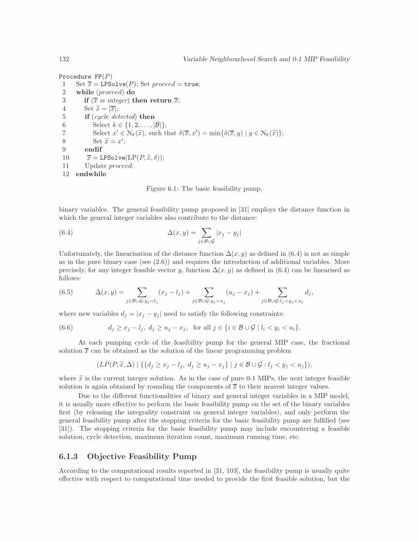
132 Variable Neighbourhood Search and 0-1 MIP Feasibility
Procedure FP(P )1 Set x = LPSolve(P ); Set proceed = true;2 while (proceed) do3 if (x is integer) then return x;4 Set x = [x];5 if (cycle detected) then6 Select k ∈ {1, 2, . . . , |B|};7 Select x′ ∈ Nk(x), such that δ(x, x′) = min{δ(x, y) | y ∈ Nk(x)};8 Set x = x′;9 endif10 x = LPSolve(LP(P, x, δ));11 Update proceed;12 endwhile
Figure 6.1: The basic feasibility pump.
binary variables. The general feasibility pump proposed in [31] employs the distance function inwhich the general integer variables also contribute to the distance:
(6.4) ∆(x, y) =∑
j∈B∪G
|xj − yj |
Unfortunately, the linearisation of the distance function ∆(x, y) as defined in (6.4) is not as simpleas in the pure binary case (see (2.6)) and requires the introduction of additional variables. Moreprecisely, for any integer feasible vector y, function ∆(x, y) as defined in (6.4) can be linearised asfollows:
(6.5) ∆(x, y) =∑
j∈B∪G:yj=lj
(xj − lj) +∑
j∈B∪G:yj=uj
(uj − xj) +∑
j∈B∪G:lj<yj<uj
dj ,
where new variables dj = |xj − yj | need to satisfy the following constraints:
(6.6) dj ≥ xj − lj , dj ≥ uj − xj , for all j ∈ {i ∈ B ∪ G | li < yi < ui}.
At each pumping cycle of the feasibility pump for the general MIP case, the fractionalsolution x can be obtained as the solution of the linear programming problem
(LP (P, x, ∆) | {{dj ≥ xj − lj , dj ≥ uj − xj} | j ∈ B ∪ G : lj < yj < uj}),
where x is the current integer solution. As in the case of pure 0-1 MIPs, the next integer feasiblesolution is again obtained by rounding the components of x to their nearest integer values.
Due to the different functionalities of binary and general integer variables in a MIP model,it is usually more effective to perform the basic feasibility pump on the set of the binary variablesfirst (by releasing the integrality constraint on general integer variables), and only perform thegeneral feasibility pump after the stopping criteria for the basic feasibility pump are fulfilled (see[31]). The stopping criteria for the basic feasibility pump may include encountering a feasiblesolution, cycle detection, maximum iteration count, maximum running time, etc.
6.1.3 Objective Feasibility Pump
According to the computational results reported in [31, 103], the feasibility pump is usually quiteeffective with respect to computational time needed to provide the first feasible solution, but the
Feasibility Pump 133
solution provided is often of a poor-quality. The reason is that original objective function is com-pletely discarded after solving the LP relaxation of the original problem in order to construct thestarting point for the search. In an attempt to provide good-quality initial solutions, a modificationof the basic FP scheme, so called objective feasibility pump, was proposed in [5]. The idea of theobjective FP is to include the original objective function as a part of the objective function of theproblem considered at a certain pumping cycle of FP. At each pumping cycle, the actual objectivefunction is computed as a linear combination of the feasibility measure and the original objectivefunction:
(6.7) ∆α(x, x) = (1− α)∆(x, x) + α
√|B ∪ G|
||c||ctx, α ∈ [0, 1],
where || · || denotes the Euclidean norm and√|B ∪ G| is the Euclidean norm of the objective
function vector (6.5). The fractional solution x at a certain iteration of the objective FP is thenobtained by solving the LP problem (LP(P, x, ∆α) | C), for the current integer solution x andcurrent value of α, where C = {{dj ≥ xj − lj, dj ≥ uj − xj} | j ∈ B ∪ G : lj < yj < uj} is theset of constraints which newly introduced variables dj need to satisfy. Furthermore, it has beenobserved in [5] that the best results are obtained if the value of α is geometrically decreased ateach iteration, i.e. if in iteration t the value αt is used, with α0 ∈ [0, 1] and αt+1 = qαt, whereq ∈ (0, 1) is a given geometric sequence ratio.
An important issue which arises with this approach is the detection of a cycle. Whereas inthe basic version of FP (both for pure binary and general integer case) visiting an integer solutionx which has already occurred in some previous iteration implies that the search process is caughtin a cycle, in the objective FP it is not necessarily the case. Indeed, since different objectivefunctions ∆αt
are used in different iterations t, changing the value of αt may force the algorithmto leave the cycle. Therefore, in the original implementation of the objective FP, a list L of pairs(x, αt) is kept for the purpose of cycle detection. Perturbation is performed at iteration t, with thecurrent integer solution x, if (x, αt′) ∈ L, t′ < t, and αt′ − αt < ε, where ε ≥ 0 is some predefinedparameter value.
Results reported in [5] indicate that this approach usually yields considerably higher-qualitysolutions than the basic FP. However, it generally requires much longer computational time.
6.1.4 Feasibility Pump and Local Branching
In [105], the local branching heuristic [104] is applied to near-feasible solutions obtained from FPin order to locate the feasible solutions. The underlying idea is to start from an infeasible initialsolution x and use local branching to gradually decrease the number of constraints which areviolated by x, until all constraints are finally satisfied.
In order to achieve this, some artificial variables are introduced. First, binary variables yi areintroduced to the 0-1 MIP model defined in (1.6), with the role to indicate the violated constraints.For each violated constraint at
i x ≥ bi, 1 ≤ i ≤ m, from the set of constraints Ax ≥ b in (1.6),variable yi is set to 1. Otherwise, if the ith constraint from Ax ≥ b in (1.6) is not violated, variableyi is set to 0. The new objective is to minimise the number of violated constraints
∑mi=1 yi.
Furthermore, additional artificial non-negative continuous variables σi and δi are introduced inorder to repair the infeasibility of x. More precisely, each constraint at
i x ≥ bi, 1 ≤ i ≤ m, from(1.6) is modified as at
i x + σi ≥ bi, while the additional constraints δiyi ≥ σi are introduced, forthe large enough preselected values δi ≥ 0. In summary, the modified problem is formulated as
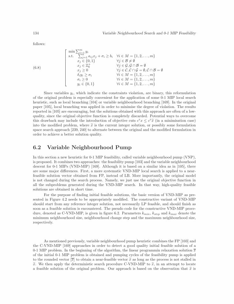
134 Variable Neighbourhood Search and 0-1 MIP Feasibility
follows:
(6.8)
min∑m
i=1 yi
s.t.∑n
j=1 aijxj + σi ≥ bi ∀i ∈M = {1, 2, . . . , m}xj ∈ {0, 1} ∀j ∈ B 6= ∅xj ∈ Z+
0 ∀j ∈ G,G ∩ B = ∅xj ≥ 0 ∀j ∈ C, C ∩ G = ∅, C ∩ B = ∅δiyi ≥ σi ∀i ∈M = {1, 2, . . . , m}σi ≥ 0 ∀i ∈M = {1, 2, . . . , m}yi ∈ {0, 1} ∀i ∈M = {1, 2, . . . , m}
Since variables yi, which indicate the constraints violation, are binary, this reformulationof the original problem is especially convenient for the application of some 0-1 MIP local searchheuristic, such as local branching [104] or variable neighbourhood branching [169]. In the originalpaper [105], local branching was applied in order to minimise the degree of violation. The resultsreported in [105] are encouraging, but the solutions obtained with this approach are often of a low-quality, since the original objective function is completely discarded. Potential ways to overcomethis drawback may include the introduction of objective cuts ctx ≤ ctx (in a minimisation case)into the modified problem, where x is the current integer solution, or possibly some formulationspace search approach [239, 240] to alternate between the original and the modified formulation inorder to achieve a better solution quality.
6.2 Variable Neighbourhood Pump
In this section a new heuristic for 0-1 MIP feasibility, called variable neighbourhood pump (VNP),is proposed. It combines two approaches: the feasibility pump [103] and the variable neighbourhooddescent for 0-1 MIPs (VND-MIP) [169]. Although it is based on a similar idea as in [105], thereare some major differences. First, a more systematic VND-MIP local search is applied to a near-feasible solution vector obtained from FP, instead of LB. More importantly, the original modelis not changed during the search process. Namely, we just use the original objective function inall the subproblems generated during the VND-MIP search. In that way, high-quality feasiblesolutions are obtained in short time.
For the purpose of finding initial feasible solutions, the basic version of VND-MIP as pre-sented in Figure 4.2 needs to be appropriately modified. The constructive variant of VND-MIPshould start from any reference integer solution, not necessarily LP feasible, and should finish assoon as a feasible solution is encountered. The pseudo code for the constructive VND-MIP proce-dure, denoted as C-VND-MIP, is given in figure 6.2. Parameters kmin, kstep and kmax denote theminimum neighbourhood size, neighbourhood change step and the maximum neighbourhood size,respectively.
As mentioned previously, variable neighbourhood pump heuristic combines the FP [103] andthe C-VND-MIP [169] approaches in order to detect a good quality initial feasible solution of a0-1 MIP problem. In the beginning of the algorithm, the linear programmin relaxation solution xof the initial 0-1 MIP problem is obtained and pumping cycles of the feasibility pump is appliedto the rounded vector [x] to obtain a near-feasible vector x as long as the process is not stalled inx. We then apply the deterministic search procedure C-VND-MIP to x, in an attempt to locatea feasible solution of the original problem. Our approach is based on the observation that x is

Variable Neighbourhood Pump 135
C-VND-MIP(P, x′, kmin, kstep, kmax)1 k = kmin; status = ‘‘noFeasibleSolFound’’;2 while (k ≤ kmax && (status == ‘‘noFeasibleSolFound’’) do3 x′′ = MIPSolve(P (k, x′), x′);4 status = getSolutionStatus(P (k, x′));5 if (status == ‘‘noFeasibleSolFound’’) then6 Add (reverse last) pseudo-cut (into) δ(x′, x) ≥ k + kstep;7 k = k + kstep;8 else9 x′ = x′′;
10 endif11 end12 return x′.
Figure 6.2: Constructive VND-MIP.
usually near-feasible and it is very likely that some feasible solution vectors can be found in somesmall neighbourhoods (with respect to Hamming distance) of x. In addition, if C-VND-MIP failsto detect the feasible solution due to the time or neighbourhood size limitations, a pseudo-cut isadded to the current subproblem in order to change the linear programming relaxation solution,and the process is iterated. If no feasible solution has been found, the algorithm reports failureand returns the last (infeasible) integer solution. The pseudo-code of the proposed VNP heuristicis given in figure 6.3.
Procedure VNP(P )1 Set proceed1 = true;2 while (proceed1) do3 Set x = LPSolve(P ); Set x = [x]; Set proceed2 = true;4 while (proceed2) do5 if (x is integer) then return x;6 x = LPSolve(LP(P, x));7 if (x 6= [x]) then x = [x]8 else Set proceed2 = false;9 endif10 endwhile11 kmin = ⌊δ(x, x)⌋; kmax = ⌊(p− kmin)/2⌋; kstep = (kmax − kmin)/5;12 x′ = VNB(P, x, kmin, kstep, kmax);13 if (x′ = x) then //VNB failed to find the feasible solution.14 P = (P | δ(x, x) ≥ kmin);15 Update proceed1;16 else return x′;17 endif18 endwhile19 Output message: ”No feasible solution found”; return x;
Figure 6.3: The variable neighbourhood pump pseudo-code.

136 Variable Neighbourhood Search and 0-1 MIP Feasibility
6.3 Constructive Variable Neighbourhood DecompositionSearch
Variable neighbourhood decomposition search for 0-1 MIPs, as described in Chapter 4, is a heuristicbased on the systematic hard variable fixing (diving) process, according to the information obtainedfrom the linear programming relaxation solution of the problem. The VNDS approach introducedin Chapter 4 can easily be adjusted to tackle the 0-1 MIP feasibility problem, by observing thata general-purpose MIP solver can be used not only for finding (near) optimal solutions of a giveninput problem, but also for finding an initial feasible solution. The resulting constructive VNDS-MIP procedure, called C-VNDS-MIP, can be described as follows.
The algorithm begins with obtaining the LP relaxation solution x of the original problemP , and generating an initial integer (not necessarily feasible) solution x = [x], by rounding the LPsolution x. Note that, if the optimal solution x is integer feasible for P , we stop and return x. Ateach iteration of the C-VNDS-MIP procedure, the distances δj =| xj−xj | from the current integersolution values (xj)j∈B to the corresponding LP relaxation solution values (xj)j∈B are computedand the variables xj , j ∈ B are indexed so that δ1 ≤ δ2 ≤ . . . ≤ δp (where p =| B |). Then thesubproblems P (x, {1, . . . , k}) obtained from the original problem P are successively solved, wherethe first k variables are fixed to their values in the current incumbent solution x. If a feasiblesolution is found by solving P (x, {1, . . . , k}), it is returned as a feasible solution of the originalproblem P . Otherwise, a pseudo-cut δ({1, . . . , k}, x, x) ≥ 1 is added in order to avoid exploringthe search space of P (x, {1, . . . , k}) again and the next subproblem is examined. If no feasiblesolution is detected after solving all subproblems P (x, {1, . . . , k}), kmin ≤ k ≤ kmax, kmin = kstep,kmax = |B|−kstep, the linear programming relaxation of the current problem P , which includes allthe pseudo-cuts added during the search process, is solved and the process is iterated. If no feasiblesolution has been found due to the fulfilment of the stopping criteria, the algorithm reports failureand returns the last (infeasible) integer solution. The pseudo-code of the proposed C-VNDS-MIPheuristic is given in figure 6.4.
6.4 Computational Results
In this section we present the computational results for our algorithms. All results reported areobtained on a computer with a 2.4GHz Intel Core 2 Duo E6600 processor and 4GB RAM, using thegeneral purpose MIP solver IBM ILOG CPLEX 11.1. Algorithms were implemented in C++ andcompiled within Microsoft Visual Studio 2005. The 83 test instances which are considered here forcomparison purposes are the same as those previously used for testing performances of the basicFP (see [103]). The detailed description of this benchmark can be found in Tables 6.1–6.2. Thefirst column in Tables 6.1–6.2 presents the instance name, whereas the second, third and fourthcolumn show the total number of variables, the number of binary variables and the number ofconstraints, respectively.
In both of the propsoed methods, the CPLEX MIP solver is used as a black-box for solvingsubproblems to feasibility. For this special purpose, the parameter CPX PARAM MIP EMPHASIS wasset to FEASIBILITY and the parameter CPX PARAM INTSOLLIM was set to 1. Since we wanted tomake an explicit comparison with FP, the FP heuristic in CPLEX as a black-box is switched off,i.e. the parameter CPX PARAM FPHEUR is set to -1. All other parameters are set to their defaultvalues. Furthermore, as we are only interested in the first feasible solution found by the CPLEXMIP solver alone, results for the CPLEX MIP solver were also generated with these parameter
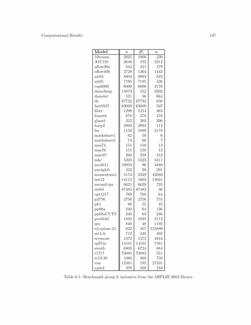
Computational Results 137
Model n |B| m10teams 2025 1800 230A1C1S1 3648 192 3312aflow30a 842 421 479aflow40b 2728 1364 1442air04 8904 8904 823air05 7195 7195 426cap6000 6000 6000 2176dano3mip 13873 552 3202danoint 521 56 664ds 67732 67732 656fast0507 63009 63009 507fiber 1298 1254 363fixnet6 878 378 478glass4 322 302 396harp2 2993 2993 112liu 1156 1089 2178markshare1 62 50 6markshare2 74 60 7mas74 151 150 13mas76 151 150 12misc07 260 259 212mkc 5325 5323 3411mod011 10958 96 4480modglob 422 98 291momentum1 5174 2349 42680net12 14115 1603 14021nsrand-ipx 6621 6620 735nw04 87482 87482 36opt1217 769 768 64p2756 2756 2756 755pk1 86 55 45pp08a 240 64 136pp08aCUTS 240 64 246protfold 1835 1835 2112qiu 840 48 1192rd-rplusc-21 622 457 125899set1ch 712 240 492seymour 1372 1372 4944sp97ar 14101 14101 1761swath 6805 6724 884t1717 73885 73885 551tr12-30 1080 360 750van 12481 192 27331vpm2 378 168 234
Table 6.1: Benchmark group I: instances from the MIPLIB 2003 library.

138 Variable Neighbourhood Search and 0-1 MIP Feasibility
Model n |B| mbiella1 7328 6110 1203NSR8K 38356 32040 6284dc1c 10039 8380 1649dc1l 37297 35638 1653dolom1 11612 9720 1803siena1 13741 11775 2220trento1 7687 6415 1265rail507 63019 63009 509rail2536c 15293 15284 2539rail2586c 13226 13215 2589rail4284c 21714 21705 4284rail4872c 24656 24645 4875A2C1S1 3648 192 3312B1C1S1 3872 288 3904B2C1S1 3872 288 3904sp97ic 12497 12497 1033sp98ar 15085 15085 1435sp98ic 10894 10894 825bg512142 792 240 1307dg012142 2080 640 6310blp-ar98 16021 15806 1128blp-ic97 9845 9753 923blp-ic98 13640 13550 717blp-ir98 6097 6031 486CMS750 4 11697 7196 16381berlin 5 8 0 1083 794 1532railway 8 1 0 1796 1177 2527usAbbrv.8.25 70 2312 1681 3291manpower1 10565 10564 25199manpower2 10009 10008 23881manpower3 10009 10008 23915manpower3a 10009 10008 23865manpower4 10009 10008 23914manpower4a 10009 10008 23866ljb2 771 681 1482ljb7 4163 3920 8133ljb9 4721 4460 9231ljb10 5496 5196 10742ljb12 4913 4633 9596
Table 6.2: Benchmark group II: the additional set of instances from [103].

Computational Results 139
C-VNDS-MIP(P, d)1 Set proceed1=proceed2=true;3 while (proceed1) do4 x = LPSolve(P ); x = [x];5 if (x == x) return x;6 δj =| xj − xj |; index xj so that δj ≤ δj+1, j = 1, . . . , p− 17 Set nd =| {j ∈ N | δj 6= 0} |, kstep = [nd/d], k = p− kstep;8 while (proceed2 and k ≥ 0) do9 Jk = {1, . . . , k}; x′ = MIPSolve(P (x, Jk), x);
10 status = getSolutionStatus(P (x, Jk));11 if (status == ‘‘noFeasibleSolFound’’) then12 P = (P | δ(Jk, x, x) ≥ 1);13 else return x′;14 if (k − kstep > p− nd) then kstep = max{[k/2], 1};15 Set k = k − kstep;16 Update proceed2;17 endwhile19 Update proceed1;20 endwhile21 Output message: ”No feasible solution found”; return x;
Figure 6.4: Constructive VNDS for 0-1 MIP feasibility.
settings, except that the parameter which controls the usage of FP is set to CPX PARAM FPHEUR=2,meaning that FP is always applied.
All three methods (VNP, C-VNDS-MIP and CPLEX MIP) were allowed 1 hour (3600 sec-onds) total running time. In addition, the time limit for solving subproblems within VND-MIP wasset to 180 seconds for all instances except van . Due to the numerical instability of this instance,a longer running time for subproblems is needed and was set to 1200 seconds. The time limit forsubproblems within C-VNDS-MIP was set to 180 seconds for all instances.
Tables 6.3–6.4 provide the results regarding the solution quality of the three methods com-pared. The first three columns contain the objective values, whereas the following three columnscontain the values of the gap from the best solution. For each instance, the gap from the bestsolution was computed according to the formula f−fbest
|fbest|× 100, where f is the observed objective
function value, and fbest is the best of the three objective values obtained by the CPLEX MIPsolver, VNP and C-VNDS-MIP, respectively. For both objective values and computational time,all methods are ranked according to their performance: rank 1 is assigned to the best method andrank 3 to the worst method (in case of ties average ranks are assigned). The objective value ranksare reported in the last three columns of Tables 6.3–6.4.
Tables 6.5–6.6 provide the results regarding the computational time of the three methodscompared. The first three columns contain the actual running times (in seconds), whereas the lastthree columns contain the running time value ranks. For the sake of robustness, the performancesof two methods are considered equal, if the difference between their running time values is lessthen 1 second.
All experimental results are summarised in Table 6.7. Number of instances solved, averagegap values and average computational time values are reported. Average rank values are alsoreported in Table 6.7 to avoid the misinterpretation of results in case that few exceptional values(either very good or very bad) influence the average scores.
From Table 6.7, we can see that the heuristics proposed in this chapter achieve a significantly
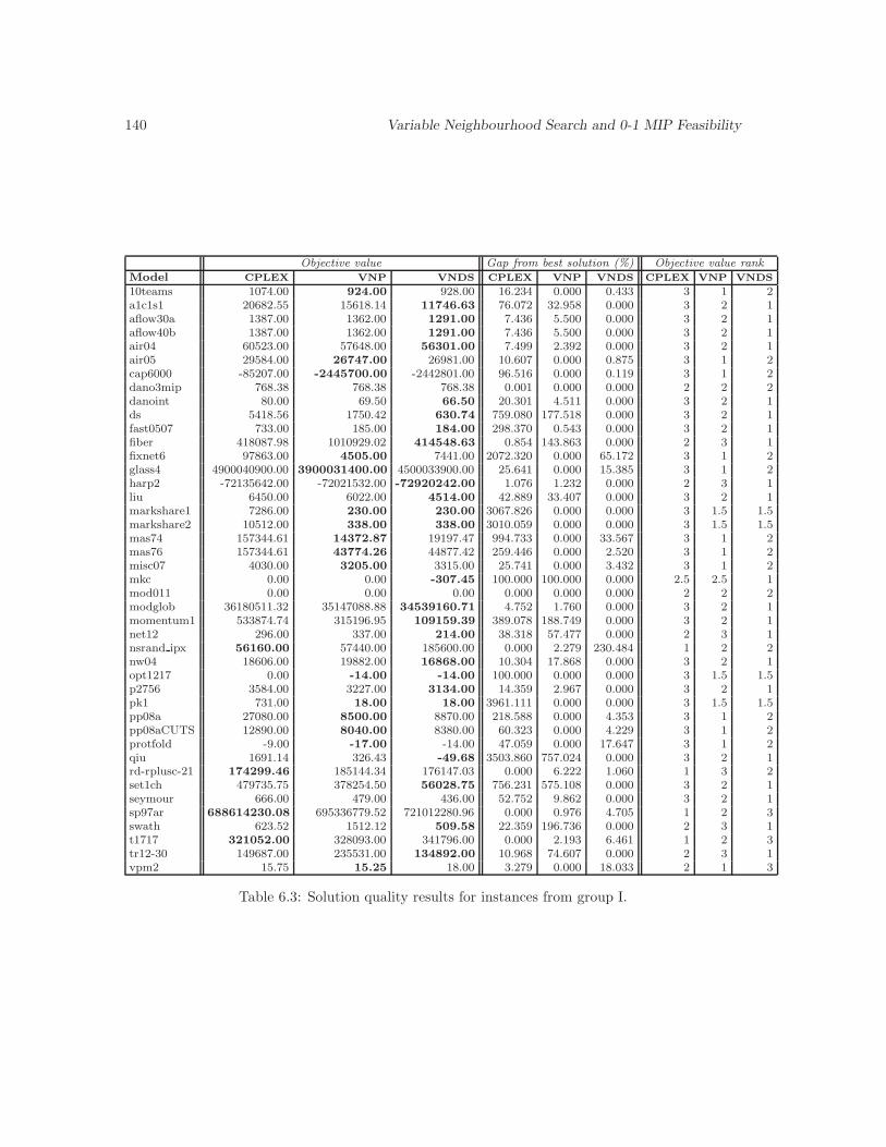
140 Variable Neighbourhood Search and 0-1 MIP Feasibility
Objective value Gap from best solution (%) Objective value rankModel CPLEX VNP VNDS CPLEX VNP VNDS CPLEX VNP VNDS
10teams 1074.00 924.00 928.00 16.234 0.000 0.433 3 1 2a1c1s1 20682.55 15618.14 11746.63 76.072 32.958 0.000 3 2 1aflow30a 1387.00 1362.00 1291.00 7.436 5.500 0.000 3 2 1aflow40b 1387.00 1362.00 1291.00 7.436 5.500 0.000 3 2 1air04 60523.00 57648.00 56301.00 7.499 2.392 0.000 3 2 1air05 29584.00 26747.00 26981.00 10.607 0.000 0.875 3 1 2cap6000 -85207.00 -2445700.00 -2442801.00 96.516 0.000 0.119 3 1 2dano3mip 768.38 768.38 768.38 0.001 0.000 0.000 2 2 2danoint 80.00 69.50 66.50 20.301 4.511 0.000 3 2 1ds 5418.56 1750.42 630.74 759.080 177.518 0.000 3 2 1fast0507 733.00 185.00 184.00 298.370 0.543 0.000 3 2 1fiber 418087.98 1010929.02 414548.63 0.854 143.863 0.000 2 3 1fixnet6 97863.00 4505.00 7441.00 2072.320 0.000 65.172 3 1 2glass4 4900040900.00 3900031400.00 4500033900.00 25.641 0.000 15.385 3 1 2harp2 -72135642.00 -72021532.00 -72920242.00 1.076 1.232 0.000 2 3 1liu 6450.00 6022.00 4514.00 42.889 33.407 0.000 3 2 1markshare1 7286.00 230.00 230.00 3067.826 0.000 0.000 3 1.5 1.5markshare2 10512.00 338.00 338.00 3010.059 0.000 0.000 3 1.5 1.5mas74 157344.61 14372.87 19197.47 994.733 0.000 33.567 3 1 2mas76 157344.61 43774.26 44877.42 259.446 0.000 2.520 3 1 2misc07 4030.00 3205.00 3315.00 25.741 0.000 3.432 3 1 2mkc 0.00 0.00 -307.45 100.000 100.000 0.000 2.5 2.5 1mod011 0.00 0.00 0.00 0.000 0.000 0.000 2 2 2modglob 36180511.32 35147088.88 34539160.71 4.752 1.760 0.000 3 2 1momentum1 533874.74 315196.95 109159.39 389.078 188.749 0.000 3 2 1net12 296.00 337.00 214.00 38.318 57.477 0.000 2 3 1nsrand ipx 56160.00 57440.00 185600.00 0.000 2.279 230.484 1 2 2nw04 18606.00 19882.00 16868.00 10.304 17.868 0.000 3 2 1opt1217 0.00 -14.00 -14.00 100.000 0.000 0.000 3 1.5 1.5p2756 3584.00 3227.00 3134.00 14.359 2.967 0.000 3 2 1pk1 731.00 18.00 18.00 3961.111 0.000 0.000 3 1.5 1.5pp08a 27080.00 8500.00 8870.00 218.588 0.000 4.353 3 1 2pp08aCUTS 12890.00 8040.00 8380.00 60.323 0.000 4.229 3 1 2protfold -9.00 -17.00 -14.00 47.059 0.000 17.647 3 1 2qiu 1691.14 326.43 -49.68 3503.860 757.024 0.000 3 2 1rd-rplusc-21 174299.46 185144.34 176147.03 0.000 6.222 1.060 1 3 2set1ch 479735.75 378254.50 56028.75 756.231 575.108 0.000 3 2 1seymour 666.00 479.00 436.00 52.752 9.862 0.000 3 2 1sp97ar 688614230.08 695336779.52 721012280.96 0.000 0.976 4.705 1 2 3swath 623.52 1512.12 509.58 22.359 196.736 0.000 2 3 1t1717 321052.00 328093.00 341796.00 0.000 2.193 6.461 1 2 3tr12-30 149687.00 235531.00 134892.00 10.968 74.607 0.000 2 3 1vpm2 15.75 15.25 18.00 3.279 0.000 18.033 2 1 3
Table 6.3: Solution quality results for instances from group I.
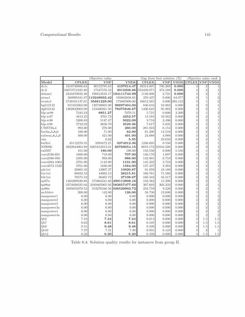
Computational Results 141
Objective value Gap from best solution (%) Objective value rankModel CPLEX VNP VNDS CPLEX VNP VNDS CPLEX VNP VNDS
dc1c 1618738986.63 36152795.63 4107014.47 39314.007 780.269 0.000 3 2 1dc1l 16673751825.80 17247576.53 3012208.66 553439.071 472.589 0.000 3 2 1dolom1 2424470932.40 199413533.17 194111743.99 1149.008 2.731 0.000 3 2 1siena1 560995341.87 119249933.42 195662038.65 370.437 0.000 64.077 3 1 2trento1 5749161137.01 35681229.00 175605900.00 16012.565 0.000 392.152 3 1 2bg512142 915353362.00 120738665.00 96697404.00 846.616 24.862 0.000 3 2 1dg012142 1202822003.00 153406921.50 78275846.67 1436.645 95.982 0.000 3 2 1blp-ar98 7243.24 6851.27 7070.51 5.721 0.000 3.200 3 1 2blp-ic97 4813.25 4701.73 4252.57 13.185 10.562 0.000 3 2 1blp-ic98 5208.83 5147.47 5022.09 3.718 2.496 0.000 3 2 1blp-ir98 2722.02 2656.70 2529.36 7.617 5.035 0.000 3 2 1CMS750 4 993.00 276.00 260.00 281.923 6.154 0.000 3 2 1berlin 5 8 0 100.00 71.00 62.00 61.290 14.516 0.000 3 2 1railway 8 1 0 500.00 421.00 401.00 24.688 4.988 0.000 3 2 1van 6.62 5.35 23.633 0.000 3 2 1biella1 45112270.55 3393472.21 3374912.36 1236.695 0.550 0.000 3 2 1NSR8K 4933944064.89 6201012913.01 60769054.15 8019.172 10104.228 0.000 2 3 1rail507 451.00 180.00 190.00 150.556 0.000 5.556 3 1 2core2536-691 1698.00 719.00 707.00 140.170 1.697 0.000 3 2 1core2586-950 2395.00 993.00 986.00 142.901 0.710 0.000 3 2 1core4284-1064 2701.00 1142.00 1101.00 145.322 3.724 0.000 3 2 1core4872-1529 3761.00 1636.00 1584.00 137.437 3.283 0.000 3 2 1a2c1s1 20865.33 12907.27 10920.87 91.059 18.189 0.000 3 2 1b1c1s1 69933.52 44983.15 26215.81 166.761 71.588 0.000 3 2 1b2c1s1 70575.52 36465.72 27108.67 160.343 34.517 0.000 3 2 1sp97ic 1464309330.88 575964341.60 499112908.16 193.382 15.398 0.000 3 2 1sp98ar 2374928235.04 2349465005.92 582657477.60 307.603 303.233 0.000 3 2 1sp98ic 1695655079.52 553276346.56 506529902.72 234.759 9.229 0.000 3 2 1usAbbrv 200.00 142.00 126.00 58.730 12.698 0.000 3 2 1manpower1 6.00 6.00 6.00 0.000 0.000 0.000 2 2 2manpower2 6.00 6.00 6.00 0.000 0.000 0.000 2 2 2manpower3 6.00 6.00 6.00 0.000 0.000 0.000 2 2 2manpower3a 6.00 6.00 6.00 0.000 0.000 0.000 2 2 2manpower4 6.00 6.00 6.00 0.000 0.000 0.000 2 2 2manpower4a 6.00 6.00 6.00 0.000 0.000 0.000 2 2 2ljb2 7.24 7.24 7.24 0.014 0.000 0.000 3 1.5 1.5ljb7 8.62 8.61 8.61 0.105 0.000 0.000 3 1.5 1.5ljb9 9.51 9.48 9.48 0.338 0.000 0.000 3 1.5 1.5ljb10 7.37 7.31 7.30 0.931 0.123 0.000 3 2 1ljb12 6.22 6.20 6.20 0.339 0.000 0.000 3 1.5 1.5
Table 6.4: Solution quality results for instances from group II.
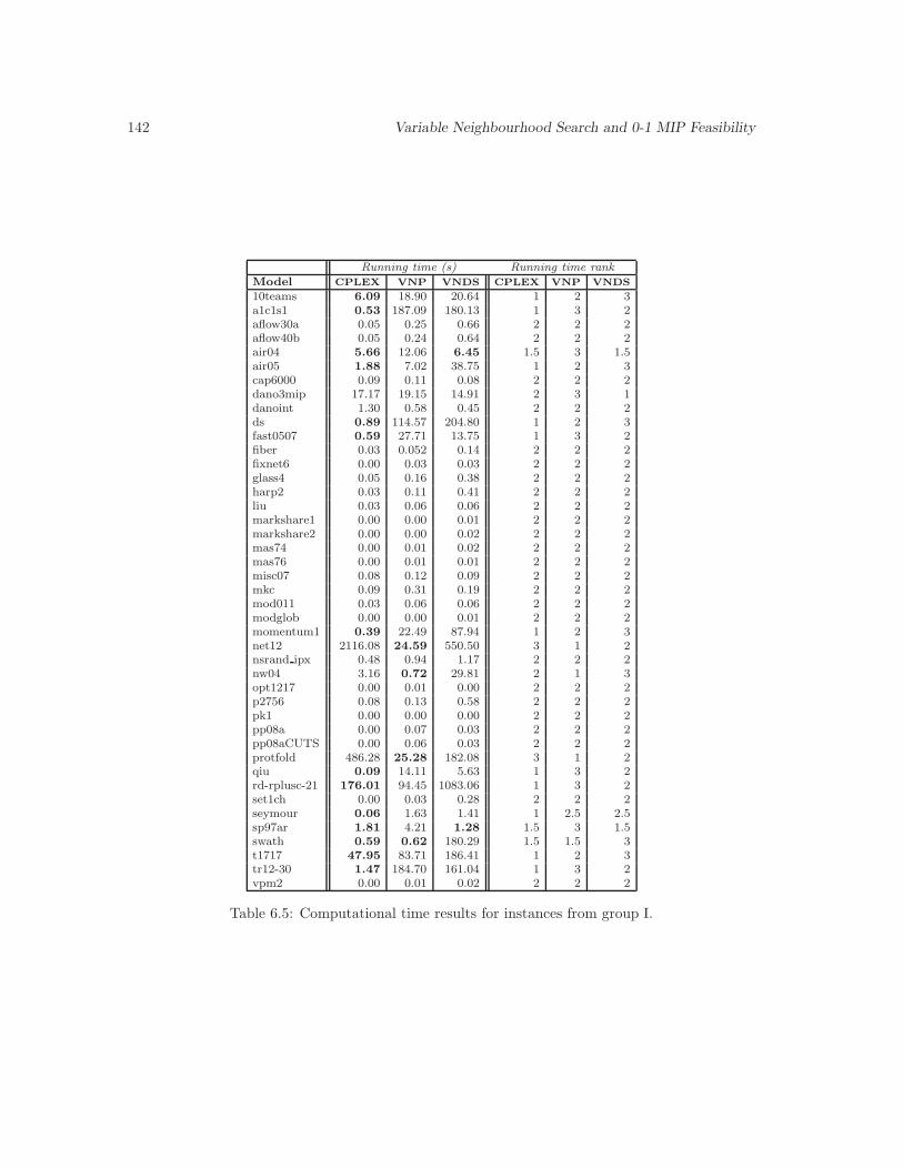
142 Variable Neighbourhood Search and 0-1 MIP Feasibility
Running time (s) Running time rankModel CPLEX VNP VNDS CPLEX VNP VNDS
10teams 6.09 18.90 20.64 1 2 3a1c1s1 0.53 187.09 180.13 1 3 2aflow30a 0.05 0.25 0.66 2 2 2aflow40b 0.05 0.24 0.64 2 2 2air04 5.66 12.06 6.45 1.5 3 1.5air05 1.88 7.02 38.75 1 2 3cap6000 0.09 0.11 0.08 2 2 2dano3mip 17.17 19.15 14.91 2 3 1danoint 1.30 0.58 0.45 2 2 2ds 0.89 114.57 204.80 1 2 3fast0507 0.59 27.71 13.75 1 3 2fiber 0.03 0.052 0.14 2 2 2fixnet6 0.00 0.03 0.03 2 2 2glass4 0.05 0.16 0.38 2 2 2harp2 0.03 0.11 0.41 2 2 2liu 0.03 0.06 0.06 2 2 2markshare1 0.00 0.00 0.01 2 2 2markshare2 0.00 0.00 0.02 2 2 2mas74 0.00 0.01 0.02 2 2 2mas76 0.00 0.01 0.01 2 2 2misc07 0.08 0.12 0.09 2 2 2mkc 0.09 0.31 0.19 2 2 2mod011 0.03 0.06 0.06 2 2 2modglob 0.00 0.00 0.01 2 2 2momentum1 0.39 22.49 87.94 1 2 3net12 2116.08 24.59 550.50 3 1 2nsrand ipx 0.48 0.94 1.17 2 2 2nw04 3.16 0.72 29.81 2 1 3opt1217 0.00 0.01 0.00 2 2 2p2756 0.08 0.13 0.58 2 2 2pk1 0.00 0.00 0.00 2 2 2pp08a 0.00 0.07 0.03 2 2 2pp08aCUTS 0.00 0.06 0.03 2 2 2protfold 486.28 25.28 182.08 3 1 2qiu 0.09 14.11 5.63 1 3 2rd-rplusc-21 176.01 94.45 1083.06 1 3 2set1ch 0.00 0.03 0.28 2 2 2seymour 0.06 1.63 1.41 1 2.5 2.5sp97ar 1.81 4.21 1.28 1.5 3 1.5swath 0.59 0.62 180.29 1.5 1.5 3t1717 47.95 83.71 186.41 1 2 3tr12-30 1.47 184.70 161.04 1 3 2vpm2 0.00 0.01 0.02 2 2 2
Table 6.5: Computational time results for instances from group I.
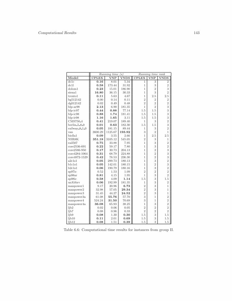
Computational Results 143
Running time (s) Running time rankModel CPLEX VNP VNDS CPLEX VNP VNDS
dc1c 0.16 8.01 5.34 1 3 2dc1l 0.58 173.44 31.92 1 3 2dolom1 0.23 15.01 186.90 1 2 3siena1 16.80 36.15 30.33 1 3 2trento1 0.11 5.63 4.67 1 2.5 2.5bg512142 0.00 0.14 0.11 2 2 2dg012142 0.02 0.49 0.48 2 2 2blp-ar98 2.13 6.90 181.35 1 2 3blp-ic97 0.44 0.88 77.14 1.5 1.5 3blp-ic98 0.88 1.74 181.41 1.5 1.5 3blp-ir98 1.16 1.65 3.11 1.5 1.5 3CMS750 4 0.41 219.07 189.40 1 3 2berlin 5 8 0 0.01 0.63 182.30 1.5 1.5 3railway 8 1 0 0.05 181.15 89.44 1 3 2van 3600.29 1125.67 193.92 3 2 1biella1 0.09 3.55 2.66 1 2.5 2.5NSR8K 351.18 3105.12 545.05 2 3 1rail507 0.75 33.88 7.95 1 3 2core2536-691 0.22 59.17 7.80 1 3 2core2586-950 0.17 30.73 204.13 1 2 3core4284-1064 0.31 68.79 224.88 1 2 3core4872-1529 0.42 78.53 236.30 1 2 3a2c1s1 0.05 299.73 180.13 1 3 2b1c1s1 0.05 142.01 180.15 1 2 3b2c1s1 0.06 190.79 180.16 1 3 2sp97ic 0.52 1.53 1.09 2 2 2sp98ar 0.81 4.15 1.95 1 3 2sp98ic 0.58 4.09 1.14 1.5 3 1.5usAbbrv 0.06 192.99 181.35 1 3 2manpower1 9.17 20.96 6.73 2 3 1manpower2 32.98 57.05 29.34 2 3 1manpower3 31.45 44.27 24.52 2 3 1manpower3a 61.08 55.76 57.70 3 1 2manpower4 524.24 31.50 70.69 3 1 2manpower4a 36.08 65.93 38.25 1 3 2ljb2 0.02 0.06 0.05 2 2 2ljb7 0.08 0.96 0.33 2 2 2ljb9 0.08 1.30 0.30 1.5 3 1.5ljb10 0.11 2.01 0.69 1.5 3 1.5ljb12 0.08 1.51 0.39 1.5 3 1.5
Table 6.6: Computational time results for instances from group II.
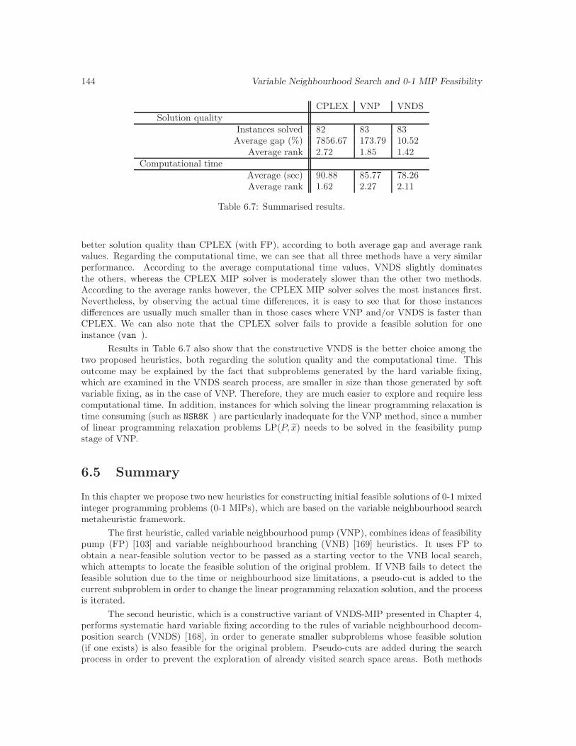
144 Variable Neighbourhood Search and 0-1 MIP Feasibility
CPLEX VNP VNDSSolution quality
Instances solved 82 83 83Average gap (%) 7856.67 173.79 10.52
Average rank 2.72 1.85 1.42Computational time
Average (sec) 90.88 85.77 78.26Average rank 1.62 2.27 2.11
Table 6.7: Summarised results.
better solution quality than CPLEX (with FP), according to both average gap and average rankvalues. Regarding the computational time, we can see that all three methods have a very similarperformance. According to the average computational time values, VNDS slightly dominatesthe others, whereas the CPLEX MIP solver is moderately slower than the other two methods.According to the average ranks however, the CPLEX MIP solver solves the most instances first.Nevertheless, by observing the actual time differences, it is easy to see that for those instancesdifferences are usually much smaller than in those cases where VNP and/or VNDS is faster thanCPLEX. We can also note that the CPLEX solver fails to provide a feasible solution for oneinstance (van ).
Results in Table 6.7 also show that the constructive VNDS is the better choice among thetwo proposed heuristics, both regarding the solution quality and the computational time. Thisoutcome may be explained by the fact that subproblems generated by the hard variable fixing,which are examined in the VNDS search process, are smaller in size than those generated by softvariable fixing, as in the case of VNP. Therefore, they are much easier to explore and require lesscomputational time. In addition, instances for which solving the linear programming relaxation istime consuming (such as NSR8K ) are particularly inadequate for the VNP method, since a numberof linear programming relaxation problems LP(P, x) needs to be solved in the feasibility pumpstage of VNP.
6.5 Summary
In this chapter we propose two new heuristics for constructing initial feasible solutions of 0-1 mixedinteger programming problems (0-1 MIPs), which are based on the variable neighbourhood searchmetaheuristic framework.
The first heuristic, called variable neighbourhood pump (VNP), combines ideas of feasibilitypump (FP) [103] and variable neighbourhood branching (VNB) [169] heuristics. It uses FP toobtain a near-feasible solution vector to be passed as a starting vector to the VNB local search,which attempts to locate the feasible solution of the original problem. If VNB fails to detect thefeasible solution due to the time or neighbourhood size limitations, a pseudo-cut is added to thecurrent subproblem in order to change the linear programming relaxation solution, and the processis iterated.
The second heuristic, which is a constructive variant of VNDS-MIP presented in Chapter 4,performs systematic hard variable fixing according to the rules of variable neighbourhood decom-position search (VNDS) [168], in order to generate smaller subproblems whose feasible solution(if one exists) is also feasible for the original problem. Pseudo-cuts are added during the searchprocess in order to prevent the exploration of already visited search space areas. Both methods

Summary 145
use the generic CPLEX MIP solver as a black-box for finding feasible solutions.
The two proposed heuristics were tested on an established set of 83 benchmark problems(proven to be difficult to solve to feasibility) and compared with the IBM ILOG CPLEX 11.1MIP solver (which already includes standard FP as a primal heuristic). Based on the average bestsolution gap and average rank values, we can conclude that both methods significantly outperformthe CPLEX MIP solver regarding the solution quality. The constructive VNDS heuristic has thebest performance, with the average gap of only 10.52% and average rank 1.43, followed by VNPwith gap 173.79% and rank 1.84, whereas the CPLEX MIP solver has the worst performance, withaverage gap 7856.67% and rank 2.73. Regarding the computational time, the difference betweenthe methods is not that remarkable. Still, VNDS has the smallest average computational time(78.26 seconds), VNP is the second best method with average running time 85.77 seconds and theCPLEX MIP solver is the slowest with 90.88 seconds average running time. However, by comparingthe average computational time ranks, we can see that the CPLEX MIP solver solved most of theinstances first. Finally, it is noteworthy that both proposed heuristics successfully solved all ofthe 83 instances from the benchmark, whereas CPLEX failed to find a feasible solution for oneinstance.

146 Variable Neighbourhood Search and 0-1 MIP Feasibility

Chapter 7
Conclusions
The research reported in this thesis focuses on the development of novel variable neighbourhoodsearch (VNS) [237] based heuristics for 0-1 mixed integer programming (MIP) problems and clus-tering. The major part of this thesis is devoted to designing matheuristics for 0-1 mixed integerprogramming problems derived from the variable neighbourhood search metaheuristic. Neighbour-hood structures are implicitly defined and updated according to the set of parameters acquiredfrom the mathematical formulation of the input problem. Normally, the general-purpose CPLEXMIP solver is used as a search component within VNS. However, the aim of this thesis is not solelyto design specific heuristics for specific problems. Some new variants of the VNS metaheuristicitself are also proposed, in an endeavour to develop a more general framework, which is able toadapt to the specific features of a specific problem instance. Moreover, a new unifying perspectiveon modern advances in metaheuristics, called hyper-reactive optimisation, was proposed.
In Chapter 2, a thorough survey of the local search based metaheuristic methods was sup-plied. Most theoretical and practical aspects of neighbourhood search were covered, from thesimplest local search to the highly modern techniques, involving large-scale neighbourhood search,reactive approaches and formulation space search. Local search techniques for 0-1 MIP problemswere also studied. Apart from outlining the existing concepts and components of a neighbourhoodsearch in combinatorial optimisation, the aim of Chapter 2 was also to point out the possible futuretrends in the developments of explorative methods. The prospects of incorporating automatic com-ponent tuning, together with adaptive memory, into the search process were discussed, especiallyfor the case when not only the basic search parameters are considered, but also the different prob-lem formulations and possible neighbourhood structures. As a result, a comprehensive approachto solving combinatorial optimization problems was proposed, called hyper-reactive optimisation,which integrates the philosophies of a reactive search and a hyper-heuristic search.
Chapter 3 shows that the variable neighbourhood search (VNS) heuristic for data clusteringcan be successfully employed as a new colour image quantisation (CIQ) technique. In order to avoidlong running time of the algorithm, the decomposed (VNDS) and the reduced (RVNS) versions ofthe VNS heuristic were designed. Results obtained show that the errors of the proposed heuristicscan compare favourably to those of recently proposed heuristics from the literature, within areasonable time. In addition, the two different models for solving CIQ were compared: the M -Median model and the usual M -means model. The results of that comparison showed that theVNS based heuristic for the M -Median is much faster, even in the case when the latter use theM -Median solution as initial one. It is also shown that in the case of quantisation to large numberof colours, solutions of the same visual quality are obtained with both models. Future research inthis direction may include the use of a VNS technique for solving other similar problems such as
147

148 Conclusions
colour image segmentation [54].
In Chapter 4 a new approach for solving 0-1 MIP problems was proposed. The proposedmethod, called VNDS-MIP, combines hard and soft variable fixing: hard fixing is based on thevariable neighbourhood decomposition search framework, whereas soft fixing introduces pseudo-cuts as in local branching (LB) [104], according to the rules of the variable neighbourhood descentscheme [169]. The proposed VNDS-MIP proved to perform well when compared with the state-of-the-art 0-1 MIP solution methods and the exact CPLEX MIP solver. The current state ofthe art methods considered for the purpose of comparison with VNDS-MIP were local branching(LB) [104], variable neighbourhood branching (VNB) [169] and relaxation induced neighbourhoodsearch (RINS) [75]. The experiments showed that VNDS-MIP was the best choice among all thesolution methods compared, regarding all the aspects considered: average percentage gap, averageobjective value rank and the number of times that the method managed to improve the bestknown published objective. In addition, VNDS-MIP appeared to be the second best method (afterLB) regarding the computational time, according to both average computational time and averagetime performance rank. The conclusions about the performance of the compared algorithms werereinforced by conducting a statistical analysis on the experimental results, which proved that asignificant difference between the compared algorithms indeed exists.
Chapter 5 was dedicated to various applications of VNDS for some specific 0-1 MIP problems:the multidimensional knapsack problem (MKP), the problem of barge container ships routing andthe two-stage stochastic mixed integer programming problem (2SSP). New heuristics for solvingthe MKP were proposed, which dynamically improve lower and upper bounds on the optimalvalue within VNDS-MIP. Different heuristics were derived by choosing a particular strategy ofupdating lower and upper bounds, and thus defining different schemes for generating a seriesof sub-problems. A two-level decomposition scheme for MKP was also proposed, in which sub-problems derived using one criterion are further divided into subproblems according to anothercriterion. Furthermore, for two of the proposed heuristics convergence to an optimal solution wasproven if no limitations regarding the execution time or the number of iterations are imposed.Based on extensive computational analysis performed on benchmark instances from the literatureand several statistical tests designed for the comparison purposes, it was concluded that VNDSbased matheuristic has a lot of potential for solving MKP. In particular, the proposed algorithmsare comparable with the current state-of-the-art heuristics for MKP and a few new best knownlower bound values were obtained. For the case of the barge container ship routing problem, theuse of MIP heuristics was also proved to be beneficial, both regarding the solution quality and(especially) the execution time. The same set of solution methods was used as in Chapter 4, whichdeals with 0-1 MIP problems in general. The VNB heuristic proved to be better than the CPLEXMIP solver regarding both criteria (solution quality/execution time). LB and VNDS did notachieve as good solution quality as CPLEX, but had significantly better execution time (they wereapproximately 3 times faster than CPLEX). Based on the computational analysis performed on anestablished benchmark of 25 stochastic integer programming (SIP) instances [7], it was concludedthat the VNDS based matheuristic has a lot of potential for solving mixed integer two-stagestochastic (2SSP) problems as well. Computational results showed that the proposed VNDS-SIP
method was competitive with the CPLEX MIP solver for the deterministic equivalent problem(DEP) regarding the solution quality: it achieved the same objective value as the CPLEX MIPsolver for DEP in 15 cases, had better performance in 7 cases and worse performance in 3 cases.VNDS-SIP usually required longer execution time than the DEP solver. However, it is remarkablethat, for the three largest instances whose deterministic equivalents contain hundreds of thousandsbinary variables, VNDS-SIP obtained a significantly better objective value (approximately 200%better) than the DEP solver, within the allowed execution time of 1800 seconds reached by bothmethods. Furthermore, these objective values were very close to optimality [7].
149
In Chapter 6, two new heuristics for constructing initial feasible solutions of 0-1 mixedinteger programs (0-1 MIPs) were proposed, based on the variable neighbourhood search meta-heuristic framework. The first heuristic, called variable neighbourhood pump (VNP), combinesideas of feasibility pump (FP) [103] and variable neighbourhood branching [169]. It uses FP toobtain a near-feasible solution vector to be passed as a starting vector to the VNB local search,which attempts to locate the feasible solution of the original problem. If VNB fails to detect thefeasible solution due to the time or neighbourhood size limitations, a pseudo-cut is added to thecurrent subproblem in order to change the linear programming relaxation solution, and the processis iterated. The second heuristic, which is a constructive variant of VNDS-MIP presented in Chap-ter 4, performs systematic hard variable fixing according to the rules of variable neighbourhooddecomposition search (VNDS) [168], in order to generate smaller subproblems whose feasible solu-tion (if one exists) is also feasible for the original problem. Pseudo-cuts are added during the searchprocess in order to prevent the exploration of already visited search space areas. Both methodsuse the generic CPLEX MIP solver as a black-box for finding feasible solutions. The two proposedheuristics were tested on an established set of 83 benchmark problems (proven to be difficult tosolve to feasibility) and compared with the IBM ILOG CPLEX 11.1 MIP solver (which alreadyincludes standard FP as a primal heuristic). Based on the average best solution gap and averagerank values, it is concluded that both methods significantly outperform the CPLEX MIP solverregarding the solution quality. The constructive VNDS heuristic had the best performance, withthe average gap of only 10.52% and average rank 1.43, followed by VNP with gap 173.79% andrank 1.84, whereas the CPLEX MIP solver had the worst performance, with average gap 7856.67%and rank 2.73. Regarding the computational time, the difference between the methods was notthat remarkable. Still, VNDS had the smallest average computational time (78.26 seconds), VNPwas the second best method with average running time 85.77 seconds and the CPLEX MIP solverwas the slowest with 90.88 seconds average running time. However, by comparing the averagecomputational time ranks, one could observe that the CPLEX MIP solver managed to solve mostof the instances first. Finally, it is noteworthy that both proposed heuristics successfully solved allof the 83 instances from the benchmark, whereas CPLEX failed to find a feasible solution for oneinstance.
In summary, the research reported in this thesis and the results obtained may be of benefitto various scientific and industrial communities. On one hand, an up to date coverage of existingmetaheuristic approaches and the new solution methodologies proposed in this thesis may helpacademic researchers attempting to develop computationally effective search heuristics for large-scale discrete optimisation problems. On the other hand, practitioners from variety of areas, suchas different industries, public services, government sectors, may benefit from the applications of theproposed solution techniques to find solutions to problems arising in diverse real-world applications.In particular, the integration of some of the proposed solution methods into a general purpose MIPsolver may enhance the overall performance of that solver, thus improving its overall potential forsolving difficult real-world MIP models. For example, the integration of VNDS based heuristicfor solving the 2SSP problem into the OptiRisk FortSP stochastic programming solver has ledto promising results regarding the SP problems (see Chapter 5, Section 5.3). The theory andalgorithms presented in this thesis indicate that hybridisation of the CPLEX MIP solver and theVNS metaheuristic can be very effective for solving large instances of mixed integer programmingproblems. More generally, the results presented in this thesis suggest that hybridisation of exact(commercial) integer programming solvers and some metaheuristic methods is of high interestand such combinations deserve further practical and theoretical investigation. The author hopesthat this thesis may encourage a broader adoption of exploiting the mathematical formulations ofproblems within metaheuristic frameworks in the area of linear and mixed integer programming.

150 Conclusions

Bibliography
[1] E. Aarts, J. Korst, and W. Michiels. Simulated annealing. Search Methodologies, pages187–210, 2005.
[2] E. Aarts and J.K. Lenstra. Local search in combinatorial optimization. Princeton UniversityPress, 2003.
[3] E.H.L. Aarts, J.H.M. Korst, and P.J.M. van Laarhoven. A quantitative analysis of thesimulated annealing algorithm: A case study for the traveling salesman problem. Journal ofStatistical Physics, 50(1):187–206, 1988.
[4] E.H.L. Aarts, J.H.M. Korst, and P.J.M. Van Laarhoven. Simulated annealing. In E. Aartsand J.K. Lenstra, editors, Local search in combinatorial optimization, pages 91–120. Springer,1997.
[5] T. Achterberg and T. Berthold. Improving the feasibility pump. Discrete Optimization,4:77–86, 2007.
[6] R. Agarwal and O. Ergun. Ship scheduling and network design for cargo routing in linershipping. Transportation Science, 42:175–196, 2008.
[7] S. Ahmed. SIPLIB: A stochastic integer programming test problem library, 2004.http://www2.isye.gatech.edu/~sahmed/siplib.
[8] S. Ahmed and R. Garcia. Dynamic capacity acquisition and assignment under uncertainty.Annals of Operations Research, 124(1-4):267–283, 2004.
[9] S. Ahmed, M. Tawarmalani, and N.V. Sahinidis. A finite branch-and-bound algorithm fortwo-stage stochastic integer programs. Mathematical Programming, 100(2):355–377, 2004.
[10] R.K. Ahuja, O. Ergun, J.B. Orlin, and A.P. Punnen. A survey of very large-scale neighbor-hood search techniques. Discrete Applied Mathematics, 123(1-3):75–102, 2002.
[11] R.K. Ahuja, J.B. Orlin, and D. Sharma. Multi-exchange neighborhood structures for thecapacitated minimum spanning tree problem. Mathematical Programming, 91(1):71–97, 2001.
[12] R.K. Ahuja, J.B. Orlin, and D. Sharma. Very large-scale neighborhood search. InternationalTransactions in Operational Research, 7(4-5):301–317, 2006.
[13] R. Alvarez-Valdes, F. Parreno, and JM Tamarit. Reactive GRASP for the strip-packingproblem. Computers & Operations Research, 35(4):1065–1083, 2008.
[14] A.A. Andreatta and C.C. Ribeiro. Heuristics for the phylogeny problem. Journal of Heuris-tics, 8(4):429–447, 2002.
151

152 Bibliography
[15] F. Arito and G. Leguizamon. Incorporating Tabu Search Principles into ACO Algorithms.Hybrid Metaheuristics, 5818:130–140, 2009.
[16] G. Ausiello, P. Crescenzi, G. Gambosi, V. Kann, A. Marchetti-Spaccamela, and M. Protasi.Complexity and approximation: Combinatorial optimization problems and their approxima-bility properties. Springer Verlag, 1999.
[17] E. Balas, S. Ceria, and G. Cornuejols. Mixed 0-1 programming by lift-and-project in abranch-and-cut framework. Management Science, 42:1229–1246, 1996.
[18] E. Balas, S. Ceria, M. Dawande, F. Margot, and G. Pataki. OCTANE: A new heuristic forpure 0-1 programs. Operations Research, 49(2):207–225, 2001.
[19] E. Balas and C.H. Martin. Pivot and complement-a heuristic for 0-1 programming. Man-agement Science, pages 86–96, 1980.
[20] E. Balas, S. Schmieta, and C. Wallace. Pivot and shift–a mixed integer programming heuris-tic. Discrete Optimization, 1(1):3–12, 2004.
[21] E. Balas and E. Zemel. An algorithm for large zero-one knapsack problems. operationsResearch, pages 1130–1154, 1980.
[22] R. Battiti, M. Brunato, and F. Mascia. Reactive search and intelligent optimization. Springer,2008.
[23] R. Battiti and G. Tecchiolli. The reactive tabu search. ORSA journal on computing, 6:126–126, 1994.
[24] E. M. L. Beale. On minimizing a convex function subject to linear inequalities. Journal ofthe Royal Statistical Society, Series B, 17:173–184, 1955.
[25] J.E. Beasley. Lagrangean relaxation. In C.R. Reeves, editor, Modern heuristic techniques forcombinatorial problems, pages 243–303. Blackwell Scientific Publications, 1993.
[26] N. Belacel, P. Hansen, and N. Mladenovic. Fuzzy J-means: a new heuristic for fuzzy clus-tering. Pattern Recognition, 35(10):2193–2200, 2002.
[27] J. Ben Atkinson. A greedy look-ahead heuristic for combinatorial optimization: an appli-cation to vehicle scheduling with time windows. The Journal of the Operational ResearchSociety, 45(6):673–684, 1994.
[28] J. F. Benders. Partitioning procedures for solving mixed-variables programming problems.Numerische Mathematik, 4:238–252, 1962. Re-publised in Computational Management Sci-ence 2 (2005), 3–19.
[29] R. Bent and P. Van Hentenryck. A two-stage hybrid local search for the vehicle routingproblem with time windows. Transportation Science, 38(4):515–530, 2004.
[30] P. Berkhin. A survey of clustering data mining techniques. Grouping Multidimensional Data,pages 25–71, 2006.
[31] L. Bertacco, M. Fischetti, and A. Lodi. A feasibility pump heuristic for general mixed-integerproblems. Discrete Optimization, 4:63–76, 2007.
[32] T. Berthold. RENS – relaxation enforced neighborhood search. Technical report, ZIB-07-28.Konrad-Zuse-Zentrum fur Informationstechnik Berlin, 2008.

153
[33] D. Bertsimas and M. Sim. Robust Discrete Optimization and Network Flows. MathematicalProgramming, 98(1–3):49–71, 2003.
[34] P. Beullens, L. Muyldermans, D. Cattrysse, and D. Van Oudheusden. A guided local searchheuristic for the capacitated arc routing problem. European Journal of Operational Research,147(3):629–643, 2003.
[35] L. Bianchi, M. Dorigo, L.M. Gambardella, and W.J. Gutjahr. Metaheuristics in stochas-tic combinatorial optimization: a survey. TechReport: Dalle Molle Institute for ArtificialIntelligence, 2006.
[36] C. Blum, M.J.B. Aguilera, A. Roli, and M. Sampels, editors. Hybrid Metaheuristics: AnEmerging Approach to Optimization. Springer-Verlag, 2008.
[37] C. Blum and A. Roli. Metaheuristics in combinatorial optimization: Overview and conceptualcomparison. ACM Computing Surveys (CSUR), 35(3):268–308, 2003.
[38] E. Borger, E. Gradel, and Y. Gurevich. On the Classical Decision Problem. Springer. ISBN:978-3-540-42324-9.
[39] P. Borisovsky, A. Dolgui, and A. Eremeev. Genetic algorithms for a supply managementproblem: MIP-recombination vs greedy decoder. European Journal of Operational Research,195(3):770–779, 2009.
[40] M. Boschetti, V. Maniezzo, M. Roffilli, and A. Bolufe R”ohler. Matheuristics: Optimization, Simulation and Control. Hybrid Metaheuristics, pages171–177, 2009.
[41] S. Boussier, M. Vasquez, Y. Vimont, S. Hanafi, and P. Michelon. A multi-level search strategyfor the 0-1 multidimensional knapsack. Discrete Applied Mathematics, 158:97–109, 2010.
[42] V. Boyer, M. Elkihel, and D. El Baz. Heuristics for the 0-1 multidimensional knapsackproblem. European Journal of Operational Research, 199(3):658–664, 2009.
[43] J.P. Braquelaire and L. Brun. Comparison and optimization of methods of color imagequantization. IEEE Transactions on image processing, 6(7):1048–1052, 1997.
[44] O. Braysy. A reactive variable neighborhood search for the vehicle-routing problem withtime windows. INFORMS Journal on Computing, 15(4):347–368, 2003.
[45] J. Brimberg, P. Hansen, N. Mladenovic, and E.D. Taillard. Improvements and comparisonof heuristics for solving the uncapacitated multisource Weber problem. Operations Research,48(3):444–460, 2000.
[46] J. Brimberg, N. Mladenovic, D. Urosevic, and E. Ngai. Variable neighborhood search for theheaviest k-subgraph. Computers & Operations Research, 36(11):2885–2891, 2009.
[47] E.K. Burke and G. Kendall, editors. Search Methodologies: Introductory Tutorials in Opti-mization and Decision Support Techniques. Springer, 2005.
[48] E. Burke et. al. Hyper-heuristics: an emerging direction in modern search technology. InF. Glover and G. Kochenberger, editors, Handbook of Metaheuristics, pages 457–474. KluwerAcademic Publishers, 2003.
[49] G. Caporossi and P. Hansen. Variable neighborhood search for extremal graphs. 5. Threeways to automate finding conjectures. Discrete mathematics, 276(1-3):81–94, 2004.

154 Bibliography
[50] V. Cerny. Thermodynamical approach to the traveling salesman problem: An efficient sim-ulation algorithm. Journal of optimization theory and applications, 45(1):41–51, 1985.
[51] P. Chardaire, J.L. Lutton, and A. Sutter. Thermostatistical persistency: A powerful improv-ing concept for simulated annealing algorithms. European Journal of Operational Research,86(3):565–579, 1995.
[52] V. Chavatal. Edmonds polytopes and a hieararchy of combinatorial problems. DiscreteMathematics, 4:137–179, 1973.
[53] P. Chen, H.K. Huang, and X.Y. Dong. Iterated variable neighborhood descent algorithm forthe capacitated vehicle routing problem. Expert Systems with Applications, 37(2), 2009.
[54] H.D. Cheng, X.H. Jiang, Y. Sun, and J. Wang. Color image segmentation: advances andprospects. Pattern Recognition, 34(12):2259–2281, 2001.
[55] C.F. Chien, F.P. Tseng, and C.H. Chen. An evolutionary approach to rehabilitation patientscheduling: A case study. European Journal of Operational Research, 189(3):1234–1253,2008.
[56] K.W. Chu, Y. Deng, and J. Reinitz. Parallel Simulated Annealing by Mixing of States.Journal of Computational Physics, 148(2):646–662, 1999.
[57] P.C. Chu and J.E. Beasley. A genetic algorithm for the multidimensional knapsack problem.Journal of Heuristics, 4(1):63–86, 1998.
[58] P.C. Chu and J.E. Beasley. A genetic algorithm for the multidimensional knapsack problem.Journal of Heuristics, 4:63–86, 1998.
[59] A. Church. A note on the Entscheidungsproblem. Journal of Symbolic Logic, 1(1):40–41,1936.
[60] A. Church. An unsolvable problem of elementary number theory. American journal ofmathematics, 58(2):345–363, 1936.
[61] A. Church and J.B. Rosser. Some properties of conversion. Transactions of the AmericanMathematical Society, pages 472–482, 1936.
[62] A. Cobham. The Intrinsic Computational Difficulty of Functions. In Logic, methodologyand philosophy of science III: proceedings of the Third International Congress for Logic,Methodology and Philosophy of Science, Amsterdam 1967, page 24. North-Holland Pub. Co.,1965.
[63] COLD, via Donau, OIR, and Port of Constantza. Container liner service danube. Technicalreport, Final Report, Vienna, 2006.
[64] R.K. Congram, C.N. Potts, and S.L. van de Velde. An iterated dynasearch algorithm for thesingle-machine total weighted tardiness scheduling problem. INFORMS Journal on Comput-ing, 14(1):52–67, 2002.
[65] S.A. Cook. Characterizations of pushdown machines in terms of time-bounded computers.Journal of the ACM (JACM), 18(1):4–18, 1971.
[66] S.A. Cook. The complexity of theorem-proving procedures. In Proceedings of the third annualACM symposium on Theory of computing, page 158. ACM, 1971.

155
[67] C.E. Cortes, M. Matamala, and C. Contardo. The pickup and delivery problem with trans-fers: Formulation and a branch-and-cut solution method. European Journal of OperationalResearch, 200(3):711–724, 2010.
[68] M.C. Costa, F.R. Monclar, and M. Zrikem. Variable neighborhood decomposition searchfor the optimization of power plant cable layout. Journal of Intelligent Manufacturing,13(5):353–365, 2002.
[69] T.G. Crainic, M. Gendreau, and P. Dejax. Dynamic and stochastic models for the allocationof empty containers. Operations Research, 41(1):102–126, 1993.
[70] T.G. Crainic, M. Gendreau, P. Hansen, and N. Mladenovic. Cooperative parallel variableneighborhood search for the p-median. Journal of Heuristics, 10(3):293–314, 2004.
[71] T.G. Crainic and M. Toulouse. Parallel Strategies for Metaheuristics. In F. Glover andG. Kochenberger, editors, Handbook of Metaheuristics, pages 475–514. Kluwer AcademicPublishers, 2003.
[72] T.G. Crainic, M. Toulouse, and M. Gendreau. Toward a taxonomy of parallel tabu searchheuristics. INFORMS Journal on Computing, 9:61–72, 1997.
[73] H.P. Crowder, E.L. Johnson, and M.W. Padberg. Solving large-scale zero-one linear pro-gramming problems. Operations Research, 31:803–834, 1983.
[74] V.D. Cung, S.L. Martins, C.C. Ribeiro, and C. Roucairol. Strategies for the parallel imple-mentation of metaheuristics. In C.C. Ribeiro and P. Hansen, editors, Essays and surveys inmetaheuristics, pages 263–308. Kluwer Academic Publisher, 2002.
[75] E. Danna, E. Rothberg, and C. Le Pape. Exploring relaxation induced neighborhoods toimprove mip solutions. Mathematical Programming, 102(1):71–90, 2005.
[76] G. Dantzig, A. Orden, and P. Wolfe. A generalized simplex method for minimizing a linearform under linear inequality constraints. Pacific Journal of Mathematics, 5(2):183–195, 1955.
[77] G. B. Dantzig. Linear programming under uncertainty. Management Science, 1:197–206,1955.
[78] G. B. Dantzig and P. Wolfe. The decomposition principle for linear programs. OperationsResearch, 8:101–111, 1960.
[79] G.B. Dantzig. Reminiscences about the origins of linear programming* 1. Operations Re-search Letters, 1(2):43–48, 1982.
[80] T. Davidovic, J. Lazic, V. Maras, and N. Mladenovic. Mip-based heuristic routing of bargecontainer ships. Submitted for publication to Transportation Science, 2010.
[81] M.C. De Souza and P. Martins. Skewed VNS enclosing second order algorithm for the degreeconstrained minimum spanning tree problem. European Journal of Operational Research,191(3):677–690, 2008.
[82] P.J. Dejax and T.G. Crainic. A review of empty flows and fleet management models in freighttransportation. Transportation Science, 21(4):227–248, 1987.
[83] A.H. Dekker. Kohonen neural networks for optimal colour quantization. Network: Compu-tation in Neural Systems, 5(3):351–367, 1994.
156 Bibliography
[84] J. Demsar. Statistical comparisons of classifiers over multiple data sets. The Journal ofMachine Learning Research, 7:1–30, 2006.
[85] G. Desaulniers, J. Desrosiers, and M.M. Solomon. Column generation. Springer Verlag, 2005.
[86] N. Di Domenica, C. Lucas, G. Mitra, and P. Valente. Stochastic programming and scenariogeneration within a simulation framework: An information perspective. IMA JMM, 20:1–38,2009.
[87] E.D. Dolan and J.J. More. Benchmarking optimization software with performance profiles.Mathematical Programming, pages 201–213, 2002.
[88] M. Dorigo, V. Maniezzo, and A. Colorni. Ant system: optimization by a colony of cooper-ating agents. IEEE Transactions on Systems, Man, and Cybernetics, Part B: Cybernetics,26(1):29–41, 1996.
[89] M. Dorigo and T. Stutzle. Ant colony optimization. the MIT Press, 2004.
[90] G. Dueck and T. Scheuer. Threshold accepting: a general purpose optimization algorithmappearing superior to simulated annealing. Journal of Computational Physics, 90(1):161–175,1990.
[91] I. Dumitrescu, S. Ropke, J.F. Cordeau, and G. Laporte. The traveling salesman problemwith pickup and delivery: polyhedral results and a branch-and-cut algorithm. MathematicalProgramming, 121(2):269–305, 2010.
[92] O.J. Dunn. Multiple comparisons among means. Journal of the American Statistical Asso-ciation, pages 52–64, 1961.
[93] M. Dyer and L. Stougie. Computational complexity of stochastic programming problems.Mathematical Programming, 106(3):423–432, 2006.
[94] J. Eckstein and M. Nediak. Pivot, Cut, and Dive: a heuristic for 0-1 mixed integer program-ming. Journal of Heuristics, 13(5):471–503, 2007.
[95] J. Edmonds. Paths, trees, and flowers. Canadian Journal of Mathematics, 17(3):449–467,1965.
[96] R.W. Eglese. Heuristics in operational research. Recent Developments in Operational Re-search, pages 49–67, 1986.
[97] M. El-Abd and M. Kamel. A taxonomy of cooperative search algorithms. Hybrid Meta-heuristics, pages 32–41, 2005.
[98] F. Ellison, G. Mitra, C. Poojari, and V. Zverovich. FortSP: A Stochas-tic Programming Solver. CARISMA, OptiRisk Systems: London, 2009.http://www.optirisk-systems.com/manuals/FortspManual.pdf.
[99] L.F. Escudero, A. Garın, M. Merino, and G. Perez. A two-stage stochastic integer pro-gramming approach as a mixture of branch-and-fix coordination and Benders decompositionschemes. Annals of Operations Research, 152(1):395–420, 2007.
[100] B.S. Everitt, S. Landau, and M. Leese. Cluster analysis. John Wiley & Sons, 2001.
[101] O. Faroe, D. Pisinger, and M. Zachariasen. Guided Local Search for the Three-DimensionalBin-Packing Problem. INFORMS Journal on Computing, 15(3):267–283, 2003.
157
[102] T.A. Feo and M.G.C. Resende. Greedy randomized adaptive search procedures. Journal ofGlobal Optimization, 6(2):109–133, 1995.
[103] M. Fischetti, F. Glover, and A. Lodi. The feasibility pump. Mathematical Programming,104:91–104, 2005.
[104] M. Fischetti and A. Lodi. Local branching. Mathematical Programming, 98(2):23–47, 2003.
[105] M. Fischetti and A. Lodi. Repairing MIP infeasibility through local branching. Computers& Operations Research, 35(5):1436–1445, 2008.
[106] M. Fischetti, C. Polo, and M. Scantamburlo. A local branching heuristic for mixed-integerprograms with 2-level variables, with an application to a telecommunication network designproblem. Networks, 44(2):61–72, 2004.
[107] C. Fleurent and F. Glover. Improved Constructive Multistart Strategies for the’QuadraticAssignment Problem Using Adaptive Memory. INFORMS Journal on Computing, 11:198–204, 1999.
[108] R. Fourer, D. M. Gay, and B. W. Kernighan. A modeling language for mathematical pro-gramming. Management Science, 36(5):519–554, 1990.
[109] A. Freville. The multidimensional 0–1 knapsack problem: An overview. European Journalof Operational Research, 155(1):1–21, 2004.
[110] A. Freville and G. Plateau. An efficient preprocessing procedure for the multidimensional0–1 knapsack problem. Disccrete Applied Mathematics, 49:189–212, 1994.
[111] A. Freville and G. Plateau. The 0-1 bidimensional knapsack problem: towards an efficienthigh-level primitive tool. Journal of Heuristics, 2:147–167, 1996.
[112] M. Friedman. A comparison of alternative tests of significance for the problem of m rankings.The Annals of Mathematical Statistics, 11(1):86–92, 1940.
[113] J. Gao, L. Sun, and M. Gen. A hybrid genetic and variable neighborhood descent algorithmfor flexible job shop scheduling problems. Computers and Operations Research, 35(9):2892–2907, 2008.
[114] F. Garcıa-Lopez, B. Melian-Batista, J.A. Moreno-Perez, and J.M. Moreno-Vega. The parallelvariable neighborhood search for the p-median problem. Journal of Heuristics, 8(3):375–388,2002.
[115] M.R. Garey, D.S. Johnson, et al. Computers and Intractability: A Guide to the Theory ofNP-completeness. WH Freeman San Francisco, 1979.
[116] B. Gavish and H. Pirkul. Efficient algorithms for solving multiconstraint zeroone knapsackproblems to optimality. Mathematical Programming, 31:78–105, 1985.
[117] M. Gendreau and J.Y. Potvin. Metaheuristics in combinatorial optimization. Annals ofOperations Research, 140(1):189–213, 2005.
[118] A.M. Geoffrion and R. Marsten. Integer programming: A framework and state-of-the-artsurvey. Management Science, 18:465–491, 1972.
158 Bibliography
[119] M. Gervautz and W. Purgathofer. A simple method for color quantization: Octree quanti-zation. In A. Glassner, editor, Graphics Gems, pages 287–293. Academic Press, New York,1990.
[120] Shubhashis Ghosh. Dins, a mip improvement heuristic. In Matteo Fischetti and David P.Williamson, editors, Proceedings of the Integer Programming and Combinatorial Optimiza-tion, volume 4513 of Lecture Notes in Computer Science, pages 310–323. Springer, 2007.
[121] F. Glover. Heuristics for Integer Programming Using Surrogate Constraints. Decision Sci-ences, 8(1):156–166, 1977.
[122] F. Glover. Future paths for integer programming and links to artificial intelligence. Com-puters and Operations Research, 13(5):533–549, 1986.
[123] F. Glover. Tabu search and adaptive memory programming: Advances, applications andchallenges. Interfaces in Computer Science and Operations Research, 1, 1996.
[124] F. Glover. Adaptive memory projection methods for integer programming. In C. Rego andB. Alidaee, editors, Metaheuristic Optimization Via Memory and Evolution, pages 425–440.Kluwer Academic Publishers, 2005.
[125] F. Glover. Parametric tabu-search for mixed integer programs. Computers & OperationsResearch, 33(9):2449–2494, 2006.
[126] F. Glover, J.P. Kelly, and M. Laguna. Genetic algorithms and tabu search: hybrids foroptimization. Computers & Operations Research, 22(1):111–134, 1995.
[127] F. Glover and G.A. Kochenberger. Critical event tabu search for multidimensional Knapsackproblems. In: Osman, I., Kelly, J. (Eds.), Meta Heuristics: Theory and Applications, pages407–427, 1996.
[128] F. Glover and G.A. Kochenberger. Handbook of metaheuristics. Springer, 2003.
[129] F. Glover and M. Laguna. General purpose heuristics for integer programmingPart I. Journalof Heuristics, 2(4):343–358, 1997.
[130] F. Glover and M. Laguna. General purpose heuristics for integer programmingPart II. Journalof Heuristics, 3(2):161–179, 1997.
[131] F. Glover, M. Laguna, et al. Tabu search. Springer, 1997.
[132] F. Glover, M. Laguna, and R. Martı. Fundamentals of scatter search and path relinking.Control and Cybernetics, 39(3):653–684, 2000.
[133] F. Glover, M. Laguna, and R. Marti. Scatter search and path relinking: Advances andapplications. International series in operations research and management science, pages1–36, 2003.
[134] F. Glover, A. Løkketangen, and D.L. Woodruff. Scatter search to generate diverse MIPsolutions. In M. Laguna and J. Gonzalez-Velarde, editors, Computing tools for modeling,optimization, and simulation: interfaces in computer science and operations research, pages299–317. Kluwer Academic Publishers, 2000.
[135] F. Glover and AP Punnen. The travelling salesman problem: new solvable cases and linkageswith the development of approximation algorithms. The Journal of the Operational ResearchSociety, 48(5):502–510, 1997.
159
[136] K. Godel, S. Feferman, J.W. Dawson, S.C. Kleene, and G.H. Moore. Collected Works:Publications 1929-1936. Oxford University Press, 1986.
[137] K.R.L. Godfrey and Y. Attikiouzel. Self-organized color image quantization for color imagedatacompression. In IEEE International Conference on Neural Networks, pages 1622–1626,1993.
[138] D.E. Goldberg. Genetic Algorithms in Search, Optimization and Machine Learning. Addison-wesley, 1989.
[139] B. Golden, L. Bodin, T. Doyle, and W. Stewart Jr. Approximate traveling salesman algo-rithms. Operations Research, 28(3):694–711, 1980.
[140] R.E. Gomory. Outline of an algorithm for integer solutions to linear programs. BulletinAmerican Mathematical Society, 64:275–278, 1958.
[141] R.E. Gomory. An algorithm for integer solutions to linear programs. In R. Graves andP. Wolfe, editors, Recent Advances in Mathematical Programming, pages 269–302. McGrawHill, New York, 1963.
[142] I.E. Grossmann. A Lagrangean based Branch-and-Cut algorithm for global optimizationof nonconvex Mixed-Integer Nonlinear Programs with decomposable structures. Journal ofGlobal Optimization, 41(2), 2008.
[143] J.M. Hammersley and D.C. Handscomb. Monte carlo methods. Taylor & Francis, 1964.
[144] R.W. Hamming. Error detecting and error correcting codes. Bell System Technical Journal,29(2):147–160, 1950.
[145] Z. Han and K.J. Ray Liu. Resource Allocation for Wireless Networks. Cambridge UniversityPress, 2008.
[146] S. Hanafi and A. Freville. An efficient tabu search approach for the 0-1 multidimensionalknapsack problem. European Journal of Operational Research, 106(2-3):659–675, 1998.
[147] S. Hanafi and A. Freville. An efficient tabu search approach for the 0–l multidimensionalknapsack problem. European Journal of Operational Research, 106:659–675, 1998.
[148] S. Hanafi, J. Lazic, and N. Mladenovic. Variable neighbourhood pump heuristic for 0-1 mixedinteger programming feasibility. Electronic Notes in Discrete Mathematics, 36:759–766, 2010.
[149] S. Hanafi, J. Lazic, N. Mladenovic, C. Wilbaut, and I. Crevits. Different variable neighbour-hood search diving strategies for multidimensional knapsack problem. Submitted to Journalof Mathematical Modelling and Algorithms, 2010.
[150] S. Hanafi, J. Lazic, N. Mladenovic, C. Wilbaut, and I. Crevits. Hybrid variable neighbour-hood decomposition search for 0-1 mixed integer programming problem. Electronic Notes inDiscrete Mathematics, 36:883–890, 2010.
[151] S. Hanafi, J. Lazic, N. Mladenovic, C. Wilbaut, and I. Crevits. Variable neighbourhood de-composition search with bounding for multidimensional knapsack problem. In N. Bakhtadzeand A. Dolgui, editors, A Proceedings volume from the 13th International Symposium onInformation Control Problems in Manufacturing, Volume 13, Part 1. 2010. ISBN: 978-3-902661-43-2, DOI: 10.3182/20090603-3-RU-2001.0502.
160 Bibliography
[152] S. Hanafi, J. Lazic, N. Mladenovic, C. Wilbaut, and I. Crevits. Variable neighbourhooddecomposition search with pseudo-cuts for multidimensional knapsack problem. Submittedto Computers & Operations Research, special issue devoted to Multidimensional KnapsackProblem, 2010.
[153] S. Hanafi and C. Wilbaut. Heuristiques convergentes basees sur des relaxations. Presentedat ROADEF 2006, Lille (France), 2006.
[154] S. Hanafi and C. Wilbaut. Improved convergent heuristics for the 0-1 multidimensionalknapsack problem. Annals of Operations Research, DOI 10.1007/s10479-009-0546-z, 2009.
[155] P. Hansen, J. Brimberg, D. Urosevic, and N. Mladenovic. Primal-dual variable neighborhoodsearch for the simple plant-location problem. INFORMS Journal on Computing, 19(4):552–564, 2007.
[156] P. Hansen, J. Brimberg, D. Urosevic, and N. Mladenovic. Solving large p-median cluster-ing problems by primal-dual variable neighborhood search . Data Mining and KnowledgeDiscovery, 19(3):351–375, 2007.
[157] P. Hansen and B. Jaumard. Cluster analysis and mathematical programming. Mathematicalprogramming, 79(1):191–215, 1997.
[158] P. Hansen, J. Lazic, and N. Mladenovic. Variable neighbourhood search for colour imagequantization. IMA Journal of Management Mathematics, 18(2):207, 2007.
[159] P. Hansen and N. Mladenovic. An Introduction to Variable Neighborhood Search. In S. Voss,S. Martello, I.H. Osman, and C. Roucairol, editors, Meta-Heuristics: Advances and Trendsin Local Search Paradigms for Optimization, pages 433–458. Kluwer Academic Publishers,1999.
[160] P. Hansen and N. Mladenovic. J-means: a new local search heuristic for minimum sum-of-squares clustering. Pattern Recognition, 34(10):405–413, 1999.
[161] P. Hansen and N. Mladenovic. Developments of Variable Neighborhood Search. In C.C.Ribeiro and P. Hansen, editors, Essays and Surveys in Metaheuristics, pages 415–440. OxfordUniversity Press, 2000.
[162] P. Hansen and N. Mladenovic. Variable neighborhood search: Principles and applications.European Journal of Operational Research, 130(3):449–467, 2001.
[163] P. Hansen and N. Mladenovic. Variable neighborhood search. In P.M. Pardalos and M.G.C.Resende, editors, Handbook of Applied Optimization, pages 221–234. Oxford University Press,2002.
[164] P. Hansen and N. Mladenovic. Variable Neighborhood Search. In F. Glover and G. Kochen-berger, editors, Handbook of Metaheuristics, pages 145–184. Kluwer Academic Publishers,2003.
[165] P. Hansen and N. Mladenovic. First vs. best improvement: An empirical study. DiscreteApplied Mathematics, 154(5):802–817, 2006.
[166] P. Hansen, N. Mladenovic, and J.A. Moreno Perez. Variable neighbourhood search: methodsand applications. 4OR: A Quarterly Journal of Operations Research, 6(4):319–360, 2008.

161
[167] P. Hansen, N. Mladenovic, and J.A. Moreno Perez. Variable neighbourhood search: methodsand applications. Annals of Operations Research, 175:367–407, 2010.
[168] P. Hansen, N. Mladenovic, and D. Perez-Britos. Variable Neighborhood DecompositionSearch. Journal of Heuristics, 7(4):335–350, 2001.
[169] P. Hansen, N. Mladenovic, and D. Urosevic. Variable neighborhood search and local branch-ing. Computers and Operations Research, 33(10):3034–3045, 2006.
[170] P. Heckbert. Color image quantization for frame buffer display. ACM SIGGRAPH ComputerGraphics, 16(3):297–307, 1982.
[171] M. Held and R.M. Karp. The travelling-salesman problem and minimum spanning trees.Operations Research, 18(6):1138–1162, 1970.
[172] M. Held and R.M. Karp. The travelling-salesman problem and minimum spanning trees:part II. Mathematical Programming, 1:6–25, 1971.
[173] D. Henderson, S.H. Jacobson, and A.W. Johnson. The theory and practice of simulatedannealing. International Series in Operations Research and Management Science, pages287–320, 2003.
[174] A. Hertz and M. Mittaz. A variable neighborhood descent algorithm for the undirectedcapacitated arc routing problem. Transportation Science, 35(4):425–434, 2001.
[175] A. Hertz, M. Plumettaz, and N. Zufferey. Variable space search for graph coloring. DiscreteApplied Mathematics, 156(13):2551–2560, 2008.
[176] F.S. Hillier. Efficient heuristic procedures for integer linear programming with an interior.Operations Research, 17(4):600–637, 1969.
[177] T. Hogg and C.P. Williams. Solving the really hard problems with cooperative search.In PROCEEDINGS OF THE NATIONAL CONFERENCE ON ARTIFICIAL INTELLI-GENCE, pages 231–231. JOHN WILEY & SONS LTD, 1993.
[178] S. Homer and A.L. Selman. Computability and complexity theory. Springer Verlag, 2001.
[179] B. Hu, M. Leitner, and G.R. Raidl. The generalized minimum edge biconnected networkproblem: Efficient neighborhood structures for variable neighborhood search. Technical re-port TR-186-1-07-02. Technische Universitat Wien, 2009.
[180] B. Hu and G.R. Raidl. Variable neighborhood descent with self-adaptive neighborhoodordering. In Proceedings of the 7th EU/MEeting on Adaptive, Self-Adaptive, and Multi-LevelMetaheuristics, 2006.
[181] M. Hussin and T. Stutzle. Hierarchical Iterated Local Search for the Quadratic AssignmentProblem. Hybrid Metaheuristics, pages 115–129, 2009.
[182] T. Ibaraki, T. Ohashi, and H. Mine. A heuristic algorithm for mixed-integer programmingproblems. Approaches to Integer Programming, pages 115–136.
[183] ILOG. Cplex 11.1. user’s manual, 2008.
[184] ILOG. CPLEX 11.2 Reference Manual. ILOG, 2008.
[185] ILOG. ILOG AMPL CPLEX System, Version 11.0, Users Guide. ILOG, 2008.

162 Bibliography
[186] R. L. Iman and J. M. Davenport. Approximations of the critical region of the Friedmanstatistic. Communications in Statistics – Theory and Methods, 9:571–595, 1980.
[187] V. Jain and I.E. Grossmann. Algorithms for hybrid MILP/CP models for a class of opti-mization problems. INFORMS Journal on computing, 13(4):258–276, 2001.
[188] D.S. Johnson and L.A. McGeoch. The traveling salesman problem: A case study in local op-timization. In E. Aarts and J.K. Lenstra, editors, Local search in combinatorial optimization,pages 215–310. Princeton University Press, 2003.
[189] D.S. Johnson, C.H. Papadimitriou, and M. Yannakakis. How easy is local search? Journalof Computer and System Sciences, 37(1):79–100, 1988.
[190] S. Jorjani, C.H. Scott, and D.L. Woodruff. Selection of an optimal subset of sizes. Interna-tional Journal of Production Research, 37(16):3697–3710, 1999.
[191] G. Joy and Z. Xiang. Center-cut for color-image quantization. The Visual Computer,10(1):62–66, 1993.
[192] R.M. Karp. Reducibility among combinatorial problems. 50 Years of Integer Programming1958-2008, pages 219–241, 1972.
[193] P. Kilby, P. Prosser, and P. Shaw. Guided local search for the vehicle routing problemwith time windows. In S. Voss, S. Martello, I.H. Osman, and C. Roucairol, editors, Meta-heuristics: Advances and Trends in Local Search Paradigms for Optimization, pages 473–486.Kluwer Academic Publishers, 1999.
[194] A. Kimms. A genetic algorithm for multi-level, multi-machine lot sizing and scheduling.Computers & operations research, 26(8):829–848, 1999.
[195] R.K. Kincaid. Solving the damper placement problem via local search heuristics. OR Spec-trum, 17(2):149–158, 1995.
[196] S. Kirkpatrick. Optimization by simulated annealing: Quantitative studies. Journal ofStatistical Physics, 34(5):975–986, 1984.
[197] R. Konings. Hub-and-spoke networks in container-on-barge transport. In Transportation Re-search Record: Journal of the Transportation Research Board, 1963, TRB, National ResearchCouncil, Washington, D.C.:23–32, 2006.
[198] K. Kostikas and C. Fragakis. Genetic programming applied to mixed integer programming.Lecture Notes in Computer Science, 3003:113–124, 2004.
[199] S. Krcevinac, M. Cangalovic, V. Kovacevic-Vujicic, and M. Martic. Operaciona istrazivanja.Fakultet Organizacionih Nauka – Beograd, 2004.
[200] M. Laguna and R. Marti. GRASP and path relinking for 2-layer straight line crossingminimization. INFORMS Journal on Computing, 11:44–52, 1999.
[201] M. Laguna and R. Marti. Scatter search. Springer, 2003.
[202] S.-W. Lam, L.-H. Lee, and Tang L.-C. An approximate dynamic programming approach forthe empty container allocation problem. Transportation Research Part C, 15:265–277, 2007.
[203] A.H. Land and A.G Doig. An automatic method for solving discrete programming problems.Econometrica, 28:497–520, 1960.
163
[204] E.L. Lawler and D.E. Wood. Branch-and-bound methods: A survey. Operations Research,14:699–719, 1966.
[205] J. Lazic, S. Hanafi, and N. Mladenovic. Variable neighbourhood search diving for 0-1 mipfeasibility. Submitted to Matheuristics 2010, the third international workshop on model-based metaheuristics, 2010.
[206] J. Lazic, S. Hanafi, N. Mladenovic, and D. Urosevic. Solving 0-1 mixed integer programswith variable neighbourhood decomposition search. In N. Bakhtadze and A. Dolgui, ed-itors, A Proceedings volume from the 13th International Symposium on Information Con-trol Problems in Manufacturing, Volume 13, Part 1. 2010. ISBN: 978-3-902661-43-2, DOI:10.3182/20090603-3-RU-2001.0501.
[207] J. Lazic, S. Hanafi, N. Mladenovic, and D. Urosevic. Variable neighbourhood decompositionsearch for 0-1 mixed integer programs. Computers & Operations Research, 37(6):1055–1067,2010.
[208] J. Lazic, N. Mladenovic, G. Mitra, and V. Zverovich. Variable neighbourhood decomposi-tion search for a two-stage stochastic mixed integer programming problem. Submitted toMatheuristics 2010, the third international workshop on model-based metaheuristics, 2010.
[209] MA Lejeune. A variable neighborhood decomposition search method for supply chain man-agement planning problems. European Journal of Operational Research, 175(2):959–976,2006.
[210] L.A. Levin. Universal sequential search problems. Problemy Peredachi Informatsii, 9(3):115–116, 1973.
[211] S. Lin and B.W. Kernighan. An effective heuristic algorithm for the traveling-salesmanproblem. Operations Research, pages 498–516, 1973.
[212] A. Løkketangen. Heuristics for 0-1 mixed-integer programming. In P.M. Pardalos and M.G.C.Resende, editors, Handbook of Applied Optimization, pages 474–477. 2002.
[213] A. Løkketangen and F. Glover. Solving zero-one mixed integer programming problems usingtabu search. European Journal of Operational Research, 106(2-3):624–658, 1998.
[214] A. Løkketangen and F. Glover. Candidate list and exploration strategies for solving 0/1 mipproblems using a pivot neighborhood. In MIC-97: meta-heuristics international conference,pages 141–154, 1999.
[215] H. Lourenco, O. Martin, and T. Stutzle. Iterated local search. In F. Glover and G. Kochen-berger, editors, Handbook of metaheuristics, pages 320–353. Kluwer Academic Publishers,2003.
[216] Y.C. Luo, M. Guignard, and C.H. Chen. A hybrid approach for integer programming combin-ing genetic algorithms, linear programming and ordinal optimization. Journal of IntelligentManufacturing, 12(5):509–519, 2001.
[217] T. Lust and J. Teghem. MEMOTS: a memetic algorithm integrating tabu search for combi-natorial multiobjective optimization. Operations Research, 42(1):3–33, 2008.
[218] J. MacQUEEN. Some methods for classification and analysis of multivariate observations.In Proceedings of the 5th Berkeley Symposium on Mathematical Statistics and Probability,pages 281–297. University of California Press, 1967.
164 Bibliography
[219] V. Maniezzo, T. Stutzle, and S. Voß, editors. Hybridizing Metaheuristics and MathematicalProgramming. Springer, 2009.
[220] V. Maras. Determining optimal transport routes of maritime and inland waterway containerships (in serbian). Master’s thesis, Faculty of Transport and Traffic Engineering, Universityof Belgrade, Serbia, 2007.
[221] V. Maras. Determining optimal transport routes of inland waterway container ships. InTransportation Research Record: Journal of the Transportation Research Board, 2062, TRB,National Research Board of the National Academies, Washington, D.C.:50–58, 2008.
[222] S. Martello and P. Toth. Upper bounds and algorithms for hard 0–1 knapsack problems.Operations Research, 45:768–778, 1997.
[223] R.K. Martin. Large Scale Linear and Integer Optimization: A Unified Approach. KluwerAcademic Publishers, 1999.
[224] S.L. Martins, M.G.C. Resende, C.C. Ribeiro, and P.M. Pardalos. A parallel GRASP forthe Steiner tree problem in graphs using a hybrid local search strategy. Journal of GlobalOptimization, 17(1):267–283, 2000.
[225] M.E. Matta. A genetic algorithm for the proportionate multiprocessor open shop. Computers& Operations Research, 36(9):2601–2618, 2009.
[226] C. Mazza. Parallel simulated annealing. Random Structures and Algorithms, 3(2):139–148,2007.
[227] C. Mendes, M. Carmelo, L. Emerson, and M. Poggi. Bounds for short covering codes andreactive tabu search. Discrete Applied Mathematics, 2009.
[228] N. Metropolis, A.W. Rosenbluth, M.N. Rosenbluth, A.H. Teller, E. Teller, et al. Equation ofstate calculations by fast computing machines. The journal of chemical physics, 21(6):1087,1953.
[229] P. Mills and E. Tsang. Guided local search for solving SAT and weighted MAX-SAT prob-lems. Journal of Automated Reasoning, 24(1):205–223, 2000.
[230] P. Mills, E. Tsang, and J. Ford. Applying an extended guided local search to the quadraticassignment problem. Annals of Operations Research, 118(1):121–135, 2003.
[231] B. Mirkin. Combinatoral Optimization in Clustering. In D.Z. Du and P.M. Pardalos, editors,Handbook of Combinatorial Optimization, pages 261–329. 1998.
[232] G. Mitra, N. Di Domenica, G. Birbilis, and P. Valente. Stochastic programming and scenariogeneration within a simulation framework: An information perspective. Decision SupportSystems, 42:2197–2218, 2007.
[233] S. Mitrovic-Minic and A. Punnen. Variable Intensity Local Search. In V. Maniezzo,T. Stutzle, and S. Voß, editors, Matheuristics: Hybridizing Metaheuristics and MathematicalProgramming, pages 245–252. Springer, 2009.
[234] Snezana Mitrovic-Minic and Abraham Punnen. Very large-scale variable neighborhood searchfor the generalized assignment problem. accepted for publication in Journal of Interdisci-plinary Mathematics, 2008.
165
[235] Snezana Mitrovic-Minic and Abraham Punnen. Very large-scale variable neighborhood searchfor the multi-resource generalized assignment problem. Discrete Optimization, 6(4):370–377,2009.
[236] L.G. Mitten. Branch-and-bound methods: General formulation and properties. OperationsResearch, 18:24–34, 1970.
[237] N. Mladenovic and P. Hansen. Variable neighborhood search. Computers and OperationsResearch, 24(11):1097–1100, 1997.
[238] N. Mladenovic, J. Petrovic, V. Kovacevic-Vujcic, and M. Cangalovic. Solving spread spec-trum radar polyphase code design problem by tabu search and variable neighborhood search.European Journal of Operational Research, 151:389–399, 2004.
[239] N. Mladenovic, F. Plastria, and D. Urosevic. Reformulation descent applied to circle packingproblems. Computers & Operations Research, 32(9):2419–2434, 2005.
[240] N. Mladenovic, F. Plastria, and D. Urosevic. Formulation space search for circle packingproblems. Lecture Notes in Computer Science, 4638:212–216, 2007.
[241] J.A. Moreno-Perez, P. Hansen, and N. Mladenovic. Parallel variable neighborhood search.Technical report G200492. GERAD., 2004.
[242] J.A. Moreno-Perez, P. Hansen, and N. Mladenovic. Parallel variable neighborhood search.In E. Alba, editor, Parallel metaheuristics: a new class of algorithms. John Wiley & Sons,New York, 2005.
[243] H. Muhlenbein. Genetic algorithms. In E. Aarts and J.K. Lenstra, editors, Local search incombinatorial optimization, pages 137–172. Princeton University Press, 2003.
[244] R.A. Murphey, P.M. Pardalos, and L.S. Pitsoulis. A parallel GRASP for the data asso-ciation multidimensional assignment problem. The IMA Volumes in Mathematics and itsApplications, 106:159–180, 1998.
[245] P. Nemenyi. Distribution-free multiple comparisons. PhD thesis, Princeton., 1963.
[246] K. Nieminen, S. Ruuth, and I. Maros. Genetic algorithm for finding a good first integersolution for MILP. Department of Computing, Imperial College, Departmental TechnicalReport 2003/4, ISSN: 14694174, 2003.
[247] L. Ntaimo and S. Sen. The million-variable “march” for stochastic combinatorial optimiza-tion. Journal of Global Optimization, 32(3):385–400, 2005.
[248] Z. Ognjanovic, U. Midic, and N. Mladenovic. A hybrid genetic and variable neighborhooddescent for probabilistic SAT problem. Lecture notes in computer science, 3636:42, 2005.
[249] M. Omran, A.P. Engelbrecht, and A. Salman. Particle swarm optimization method forimage clustering. International Journal of Pattern Recognition and Artificial Intelligence,19(3):297–322, 2005.
[250] M.G. Omran, A.P. Engelbrecht, and A. Salman. A color image quantization algorithm basedon particle swarm optimization. Informatica, 29:261–269, 2005.
[251] I.H. Osman. Metastrategy simulated annealing and tabu search algorithms for the vehiclerouting problem. Annals of Operations Research, 41(4):421–451, 1993.
166 Bibliography
[252] I.H. Osman and J.P. Kelly, editors. Metaheuristics: Theory and Applications. Kluwer Aca-demic Publishers, 1996.
[253] I.H. Osman and G. Laporte. Metaheuristics: A bibliography. Annals of Operations Research,63(5):511–623, 1996.
[254] C.H. Papadimitriou. Computational complexity. John Wiley and Sons Ltd., 2003.
[255] D.C. Paraskevopoulos, P.P. Repoussis, C.D. Tarantilis, G. Ioannou, and G.P. Prastacos.A reactive variable neighborhood tabu search for the heterogeneous fleet vehicle routingproblem with time windows. Journal of Heuristics, 14(5):425–455, 2008.
[256] P. Pardalos, L. Pitsoulis, and M. Resende. A parallel GRASP for MAX-SAT problems.Applied Parallel Computing Industrial Computation and Optimization, pages 575–585, 1996.
[257] P.M. Pardalos, L.S. Pitsoulis, and M.G.C. Resende. A parallel GRASP implementation forthe quadratic assignment problem. In A. Ferreira and J. Rolim, editors, Parallel Algorithmsfor Irregularly Structured Problems – Irregular ’94, pages 115–133. Kluwer Academic Pub-lisher, 1995.
[258] D. Pisinger. An expanding-core algorithm for the exact 0–1 knapsack problem. EuropeanJournal of Operational Research, 87:175–187, 1995.
[259] D. Pisinger. An expanding-core algorithm for the exact 0-1 knapsack problem. EuropeanJournal of Operational Research, 87(1):175–187, 1995.
[260] L.S. Pitsoulis and M.G.C. Resende. Greedy randomized adaptive search procedures. In P.M.Pardalos and M.G.C. Resende, editors, Handbook of Applied Optimization, pages 168–183.Oxford University Press, 2002.
[261] G. Plateau and M. Elkihel. A hybrid method for the 0–1 knapsack problem. Methods ofOperations Research, 49:277–293, 1985.
[262] G. Polya. How to solve it. Princeton University Press, 1948.
[263] M. Prais and CC Ribeiro. Parameter variation in GRASP procedures. Investigacion Opera-tiva, 9:1–20, 2000.
[264] M. Prais and C.C. Ribeiro. Reactive GRASP: An application to a matrix decompositionproblem in TDMA traffic assignment. INFORMS Journal on Computing, 12(3):164–176,2000.
[265] P. Preux and E.G. Talbi. Towards hybrid evolutionary algorithms. International Transactionsin Operational Research, 6(6):557–570, 1999.
[266] J. Puchinger and G.R. Raidl. Combining Metaheuristics and Exact Algorithms in Combi-natorial Optimization: A Survey and Classification. Lecture Notes in Computer Science,3562:41–53, 2005.
[267] J. Puchinger and G.R. Raidl. Bringing order into the neighborhoods: Relaxation guidedvariable neighborhood search. Journal of Heuristics, 14(5):457–472, 2008.
[268] J. Puchinger and G.R. Raidl. Combining (integer) linear programming techniques and meta-heuristics for combinatorial optimization. In C. Blum, M.J.B. Aguilera, A. Roli, and M. Sam-pels, editors, Hybrid metaheuristics: an emerging approach to optmization, pages 31–62.Springer-Verlag, 2008.

167
[269] J. Puchinger, G.R. Raidl, and U. Pferschy. The core concept for the multidimensional knap-sack problem. Lecture Notes in Computer Science, 3906:195–208, 2006.
[270] Z. Radmilovic. Inland Waterway Transport (In Serbian). Faculty of Transport and TrafficEngineering, University of Belgrade, Serbia, 2007.
[271] G.R. Raidl. An improved genetic algorithm for the multiconstrained 0–1 knapsack problem.In Proceedings of the 5th IEEE International Conference on Evolutionary Computation, pages207–211. Citeseer, 1998.
[272] G.R. Raidl. A unified view on hybrid metaheuristics. Lecture Notes in Computer Science,4030:1–12, 2006.
[273] K. Rana and R. G. Vickson. A model and solution algorithm for optimal routing of atime-chartered containership. Transportation Science, 22(2):83–95, 1988.
[274] K. Rana and R. G. Vickson. Routing container ships using lagrangean relaxation and de-composition. Transportation Science, 25(3):201–214, 1991.
[275] S. Rayward, I. Osman, C. Reeves, and G. Smith. Modern heuristic search methods. JohnWiley & Sons, Chichester, England, 1996.
[276] C.R. Reeves and J.E. Beasley. Modern heuristic techniques for combinatorial problems. JohnWiley & Sons, New York, 1993.
[277] C.R. Reeves and J.E. Rowe. Genetic algorithms – principles and perspectives. Kluwer Aca-demic Publishers, 2003.
[278] S. Remde, P. Cowling, K. Dahal, and N. Colledge. Exact/heuristic hybrids using rVNSand hyperheuristics for workforce scheduling. Evolutionary Computation in CombinatorialOptimization, pages 188–197, 2007.
[279] P. Repoussis, D. Paraskevopoulos, C. Tarantilis, and G. Ioannou. A reactive greedy random-ized variable neighborhood tabu search for the vehicle routing problem with time windows.Lecture Notes in Computer Science, 4030:124–138, 2006.
[280] M. Resende and C. Ribeiro. Greedy randomized adaptive search procedures. In F. Gloverand G. Kochenberger, editors, Handbook of metaheuristics, pages 219–249. Kluwer AcademicPublishers, 2003.
[281] Online resource. New world encyclopedia. http://www.newworldencyclopedia.org.
[282] C. Ribeiro and P. Hansen. Essays and surveys in metaheuristics. Kluwer Academic Publish-ers, 2002.
[283] C.C. Ribeiro and M.C. Souza. Variable neighborhood search for the degree-constrainedminimum spanning tree problem. Discrete Applied Mathematics, 118(1-2):43–54, 2002.
[284] E. Rothberg. An evolutionary algorithm for polishing mixed integer programming solutions.INFORMS Journal on Computing, 19:1436–1445, 2007.
[285] S. Salhi. A perturbation heuristic for a class of location problems. Journal of OperationsResearch Society, 48(12):1233–1240, 1997.
[286] S. Salhi and M. Sari. A multi-level composite heuristic for the multi-depot vehicle fleet mixproblem* 1. European Journal of Operational Research, 103(1):95–112, 1997.
168 Bibliography
[287] R.M. Saltzman and F.S. Hillier. A heuristic ceiling point algorithm for general integer linearprogramming. Management Science, 38(2):263–283, 1992.
[288] P. Scheunders. A genetic c-means clustering algorithm applied to color image quantization.Pattern Recognition, 30(6):859–866, 1997.
[289] L. Schrage. Optimization Modeling with LINGO. sixth edition, LINDO Systems, Inc., 2006.
[290] A. Schrijver. Theory of linear and integer programming. John Wiley & Sons Inc, 1998.
[291] R. Schultz, L. Stougie, and M.H. Van Der Vlerk. Two-stage stochastic integer programming:a survey. Statistica Neerlandica, 50(3):404–416, 1996.
[292] S. Sen and H.D. Sherali. Decomposition with branch-and-cut approaches for two-stagestochastic mixed-integer programming. Mathematical Programming, 106(2):203–223, 2006.
[293] Z. Sevkli and F. Sevilgen. A hybrid particle swarm optimization algorithm for functionoptimization. Lecture Notes in Computer Science, 4974:585–595, 2008.
[294] P. Shaw. Using Constraint Programming and Local Search Methods to Solve Vehicle RoutingProblems. Lecture Notes in Computer Science, pages 417–431, 1998.
[295] K. Shintani, A. Imai, E. Nishimura, and S. Papadimitriou. The container shipping net-work design problem with empty container repositioning. Transportation Research Part E:Logistics and Transportation Review, 43(1):39–59, 2007.
[296] E.A. Silver. An overview of heuristic solution methods. The Journal of the OperationalResearch Society, 55(9):936–956, 2004.
[297] Y. Sirisathitkul, S. Auwatanamongkol, and B. Uyyanonvara. Color image quantization usingdistances between adjacent colors along the color axis with highest color variance. PatternRecognition Letters, 25(9):1025–1043, 2004.
[298] A.L. Soyster, B. Lev, and W. Slivka. Zero-One Programming with Many Variables and FewConstraints. European Journal of Operational Research, 2(3):195–201, 1978.
[299] G.J. Stigler. The cost of subsistence. American Journal of Agricultural Economics, 27(2):303,1945.
[300] T. Stutzle. Iterated local search for the quadratic assignment problem. European Journal ofOperational Research, 174(3):1519–1539, 2006.
[301] E.D. Taillard, L.M. Gambardella, M. Gendreau, and J.Y. Potvin. Adaptive memory pro-gramming: A unified view of metaheuristics. European Journal of Operational Research,135(1):1–16, 2001.
[302] E.G. Talbi. A taxonomy of hybrid metaheuristics. Journal of heuristics, 8(5):541–564, 2002.
[303] L. Tang and X. Wang. Iterated local search algorithm based on very large-scale neighbor-hood for prize-collecting vehicle routing problem. The International Journal of AdvancedManufacturing Technology, 29(11):1246–1258, 2006.
[304] D. Thierens. Adaptive Operator Selection for Iterated Local Search. Engineering StochasticLocal Search Algorithms. Designing, Implementing and Analyzing Effective Heuristics, pages140–144, 2009.

169
[305] P.M. Thompson and H.N. Psaraftis. Cyclic transfer algorithms for multivehicle routing andscheduling problems. Operations Research, pages 935–946, 1993.
[306] M. Toulouse, K. Thulasiraman, and F. Glover. Multi-level cooperative search: A newparadigm for combinatorial optimization and an application to graph partitioning. Euro-Par99 Parallel Processing, pages 533–542, 1999.
[307] A.M. Turing. On computable numbers, with an application to the Entscheidungsproblem.Proceedings of the London Mathematical Society, 2(43):230–265, 1936.
[308] D. Urosevic, J. Brimberg, and N. Mladenovic. Variable neighborhood decomposition searchfor the edge weighted k-cardinality tree problem. Computers & Operations Research,31(8):1205–1213, 2004.
[309] P. Vansteenwegen, W. Souffriau, G.V. Berghe, and D.V. Oudheusden. A guided local searchmetaheuristic for the team orienteering problem. European journal of operational research,196(1):118–127, 2009.
[310] M. Vasquez and J. K. Hao. Une approche hybride pour le sac–a–dos multidimensionnel envariables 0–1. RAIRO Operations Research, 35:415–438, 2001.
[311] M. Vasquez and Y. Vimont. Improved results on the 0–1 multidimensional knapsack problem.European Journal of Operational Research, 165:70–81, 2005.
[312] V.V. Vazirani. Approximation algorithms. Springer, 2004.
[313] M.G.A. Verhoeven and E.H.L. Aarts. Parallel local search. Journal of Heuristics, 1(1):43–65,1995.
[314] Y. Vimont, S. Boussier, and M. Vasquez. Reduced costs propagation in an efficient im-plicit enumeration for the 01 multidimensional knapsack problem. Journal of CombinatorialOptimization, 15:165–178, 2008.
[315] J. Von Neumann. The general and logical theory of automata. Cerebral mechanisms inbehavior, pages 1–41, 1951.
[316] J. Von Neumann. The theory of automata: Construction, reproduction, homogeneity. Un-published manuscript, 1953.
[317] S. Voss, I.H. Osman, and C. Roucairol. Meta-heuristics: Advances and trends in local searchparadigms for optimization. Kluwer Academic Publishers Norwell, MA, USA, 1999.
[318] C. Voudouris and E. Tsang. Guided local search and its application to the traveling salesmanproblem. European journal of operational research, 113(2):469–499, 1999.
[319] C. Voudouris and E. Tsang. Guided local search. In F. Glover and G. Kochenberger, editors,Handbook of metaheuristics, pages 185–218. Kluwer Academic Publishers, 2003.
[320] K. Wagner and G. Wechsung. Computational complexity. Springer, 1986.
[321] S. W. Wallace and W. T. Ziemba, editors. Applications of Stochastic Programming. Societyfor Industrial and Applied Mathematic, 2005.
[322] S.J. Wan, P. Prusinkiewicz, and S.K.M. Wong. Variance-based color image quantization forframe buffer display. Color Research & Application, 15(1):52–58, 2007.

170 Bibliography
[323] N.A. Wassan, A.H. Wassan, and G. Nagy. A reactive tabu search algorithm for the ve-hicle routing problem with simultaneous pickups and deliveries. Journal of CombinatorialOptimization, 15(4):368–386, 2008.
[324] R. J. B. Wets. Stochastic programs with fixed recourse: The equivalent deterministic pro-gram. SIAM Review, 16:309–339, 1974.
[325] C. Wilbaut. Heuristiques Hybrides pour la Resolution de Problemes en Variables 0-1 Mixtes.PhD thesis, Universite de Valenciennes, Valenciennes, France, 2006.
[326] C. Wilbaut and S. Hanafi. New convergent heuristics for 0–1 mixed integer programming.European Journal of Operational Research, 195(1):62–74, 2009.
[327] C. Wilbaut, S. Hanafi, A. Freville, and S. Balev. Tabu search: global intensification usingdynamic programming. Control and Cybernetics, 35(3):579, 2006.
[328] C. Wilbaut, S. Hanafi, and S. Salhi. A survey of effective heuristics and their applicationto a variety of knapsack problems. IMA Journal of Management Mathematics, 19:227–244,2008.
[329] C. Wilbaut, S. Salhi, and S. Hanafi. An iterative variable-based fixation heuristic for the 0-1multidimensional knapsack problem. European Journal of Operational Research, 199(2):339–348, 2009.
[330] D.H. Wolpert and W.G. Macready. No free lunch theorems for optimization. IEEE transac-tions on evolutionary computation, 1(1):67–82, 1997.
[331] L.A. Wolsey and G.L. Nemhauser. Integer and Combinatorial Optimization. John Wiley&Sons, 1999.
[332] Z. Xiang and G. Joy. Color image quantization by agglomerative clustering. IEEE ComputerGraphics and Applications, 14(3):48, 1994.
[333] R. Xu and D. Wunsch. Survey of clustering algorithms. IEEE Transactions on NeuralNetworks, 16(3):645–678, 2005.
[334] M. Yazdani, M. Zandieh, and M. Amiri. Flexible job-shop scheduling with parallel variableneighborhood search algorithm. Expert Systems with Applications, 2009.
[335] V. Yigit, M.E. Aydin, and O. Turkbey. Solving large-scale uncapacitated facility locationproblems with evolutionary simulated annealing. International Journal of Production Re-search, 44(22):4773–4791, 2006.
[336] S.H. Zanakis, J.R. Evans, and A.A. Vazacopoulos. Heuristic methods and applications: acategorized survey. European Journal of Operational Research, 43(1):88–110, 1989.
[337] Y. Zhong and M.H. Cole. A vehicle routing problem with backhauls and time windows: aguided local search solution. Transportation Research Part E: Logistics and TransportationReview, 41(2):131–144, 2005.
[338] V. Zverovich, C. I. Fabian, F. Ellison, and G. Mitra. A computational study of a solversystem for processing two-stage stochastic linear programming problems. Published in theSPEP: Stochastic programming e-print series of COSP and submitted to Mathematical Pro-gramming Computation, 2009.
Index
2SSP, see mixed integer programming problem,two-stage stochastic
approximate algorithm, 4approximation algorithm, 4, 5aspiration criteria, 27
B&B, see branch-and-boundB&C, see branch-and-cutbarge container ship, 112–116
route, 113routing, 18, 87, 112–114, 148
binding set, 43, 67branch-and-bound, 12, 13, 49, 98, 123branch-and-cut, 12, 15, 71, 123branch-and-price, 16BVNS, see basic variable neighbourhood search
C-means, 56candidate
list, 13, 14, 16problem, 13, 14, 16
CIQ, see colour image quantisationcluster, 17, 53, 55, 57, 58clustering, 11, 17, 18, 53–55, 63, 147
agglomerative, 17divisive, 17hierarchical, 17partitional, 17
colour image quantisation, 18, 53, 57, 63, 147column generation, 16constraint, 3, 6, 7, 11, 12, 14, 15, 18, 19, 41, 43,
71, 96, 117, 124, 129, 132–134, 136aggregate, 15
cooling schedule, 25, 26, 33core problems, 67cut, see valid inequality, 94, 95
C-G, see Chavatal-Gomory cutChavatal-Gomory, 15objective, 92, 96, 134
cutting plane, see valid inequality
demanding problem, see computationally demand-ing MIP problem
distance, 6, 7, 34, 38, 44–47, 68, 122, 130–132,136
Hamming, 45, 135partial, 45, 122squared, 54, 57
diversification, 7, 8, 25, 27, 28, 32–36, 38, 43, 44,47, 48, 92, 100
elite solutions, 28exact algorithm, 4, 88exact method, see exact algorithmexploitation, see intensificationexploration, see diversification
fathoming, 13feasibility, see feasible solutionfeasibility pump, 10, 17, 19, 46, 129–132, 134,
144, 149basic, 131, 132general, 132objective, 132
feasibleproblem, 3region, 3, 6, 13–15, 92set, see feasible regionsolution, 3, 13, 14, 16, 21, 22, 44, 48, 49,
68, 69, 71, 89, 92–95, 98, 122, 123, 125,129–136, 144, 145, 149
first-stage problem, 121–123, 125, 127fixed neighbourhood search, 31formulation space search, 9, 40, 147FP, see feasibility pump
GLS, see guided local searchGRASP, see greedy randomised adaptive searchgreedy randomised adaptive search, 24, 28guided local search, 8, 24, 29GVNS, see general variable neighbourhood search
171

172 Index
heuristic, 4–10, 16, 18, 19, 21, 25, 28, 41, 47, 49,50, 54–61, 63, 69, 71, 73, 75, 87–89, 91–94, 100, 101, 112, 119–123, 129–131,133–136, 139, 144, 145, 147–149
hill climbing, 23hyper-heuristic, 9, 50, 147hyper-reactive, 50, 51, 131
IIRH, see iterative independent relaxation basedheuristic
ILS, see iterated local searchinfeasibility, see infeasible solutioninfeasible
problem, 3, 13, 14, 16, 69, 90, 124solution, 3, 123, 133, 135, 136
integrality gap, 13, 16, 19intensification, 7, 8, 11, 27, 28, 32, 33, 35, 36,
43, 88IRH, see iterative relaxation based heuristiciterated local search, 24, 31, 42, 123iterative independent relaxation based heuristic,
88iterative relaxation based heuristic, 88, 91
J-means, 58
K-means, 54–56, 58, 61, 63
LB, see local branchinglinear programming problem, 12, 122
mixed integer, 12pure integer, 11
local branching, 10, 11, 47, 71, 75, 81, 88, 112,118, 129, 133, 134, 148
local search, 5, 6, 8, 10, 11, 18, 21–24, 28, 31, 32,34–36, 39, 42–44, 46, 47, 50, 51, 57, 59,60, 68, 69, 73, 93, 134, 144, 147, 149
lower bound, 4, 13, 16, 19, 68, 87, 92, 95–97,99–101, 111, 112, 125, 148
LP problem, see linear programming problem
M-means, 54, 55, 57, 60–63, 147M-median, 54, 55, 57, 58, 61–63, 147mathematical programming, 3, 5, 6, 9, 11, 17,
41, 43, 88, 118matheuristic, 9–11, 18, 19, 111, 120, 123, 128,
147, 148maximal solution, 4maximum, see maximal solution
local, 22memory, 7–9, 27, 28, 43, 50
adaptive, 7, 11, 26, 50, 88, 147long term, 27, 43short term, 26, 27, 43
metaheuristic, 7–11, 13, 18, 19, 21, 23, 24, 26,28, 29, 32, 33, 35, 38–40, 42–44, 50, 51,54–56, 123, 129, 144, 147
Metropolis criterion, 24, 26, 33minimal solution, 4minimum, see minimal solution
local, 22, 35MIP problem, see mixed integer programming
problem0-1, 12, 18, 19, 44, 46, 49, 67, 81, 129–131,
134, 136, 147, 148computationally demanding, 73computationally non-demanding, 73pure 0-1, 12, 124, 129, 132
mixed integer finite basis theorem, 15mixed integer programming problem, see mixed
integer linear programming problemtwo-stage stochastic, 18, 87, 120–122, 125,
127, 128, 148move, 22–27, 38, 88, 129MP, see mathematical programming
neighbour, see neighbouring solutionneighbourhood, 6–8, 10, 11, 18, 21, 23, 26, 28,
32–36, 38, 42, 43, 46–48, 51, 56–59, 68,69, 72, 73, 88, 93, 129, 131, 134, 135,144, 147
restricted k-exchange, 43very large, 8, 11, 43
neighbourhood structure, 7, 8, 21, 22, 29, 32–34,38, 42, 43, 46, 50, 57, 122, 147
neighbourhood structures, 131neighbouring solution, 21, 23–25no free lunch, 5, 9non-demanding problem, see computationally non-
demanding MIP problem
objective function, 3, 4, 6–8, 21–26, 28, 29, 31,33, 57, 71, 74, 75, 77, 92, 93, 97, 114,129–131, 133, 134, 139
optimal solution, 4, 13, 14, 16, 22, 41, 49, 53, 57,68, 88–91, 94–98, 100, 101, 112, 117–119, 125, 131, 136, 148
locally, 22optimal value, 4, 13, 14, 68, 90, 93–95, 99, 111,
119, 148

173
optimality, 4, 5, 14, 16, 41, 69, 94, 95, 98, 100,112, 118, 124, 125, 127, 128, 130, 148
optimisation, 3combinatorial, 3, 17discrete, see combinatorial optimisationhyper-reactive, 50, 147
optimisation problem, 3, 11, 13, 21, 22, 27, 34,35, 39, 50, 90
0-1, 3combinatorial, 3, 4, 12, 21, 39, 40continuous, 3discrete, see combinatorial optimisation prob-
leminteger, 3maximisation, 3minimisation, 3mixed integer, 3
optimum, see optimal solutionlocal, see locally optimal solution
parallelisation, 7, 9, 44, 50multiple walks, 44single walk, 44
particle swarm optimisation, 55penalties, 29, 31polyhedron, 15, 121pricing problem, 16pseudo-cut, 18, 69, 81, 87, 89, 90, 92–95, 123,
124, 135, 136, 144, 148, 149PSO, see particle swarm optimisationpure 0-1 integer programming problem, 88, 89,
91, 93, 94
RCL, see restricted candidate listreactive, 8, 18, 28, 43, 50, 147recourse problem, 122reduced problem, 39, 49, 88–91, 95relaxation, 4, 7, 10–13, 19, 49, 67, 88
Lagrangian, 4, 6, 13linear programming, 7, 11, 12, 18, 88, 92,
95, 97, 121, 122, 124, 130, 134–136,144, 149
LP, see linear programming relaxation, 91MIP, 88, 91, 92tight, 13, 14
relaxation enforced neighbourhood search, 129relaxation induced neighbourhood search, 10, 11,
47, 49, 88, 148RENS, see relaxation enforced neighbourhood
search
restricted candidate list, 28restriction, 4, 8RINS, see relaxation induced neighbourhood searchRVNS, see reduced variable neighbourhood search
SA, see simulated annealingscenario, 121–123, 125, 127, 128search history, 8, 9, 26, 32, 33, 42, 43second-stage problem, see recourse problemsimulated annealing, 8, 24, 28, 50solution features, 29solution space, 3, 13, 21, 27, 32, 34, 38, 42–44,
46, 47, 50, 56, 69, 93, 94, 130, 131steepest descent, 23SVNS, see skewed variable neighbourhood search
tabu list, 26–28, 42tabu search, 8, 11, 24, 26–28, 32, 42, 43, 50, 88,
101, 108, 123TS, see tabu search
upper bound, 4, 14, 16, 91–93, 96, 111, 148
valid inequality, 15, 124variable neighbourhood branching, 19, 47, 48,
71, 88, 112, 118, 134, 144, 148, 149variable neighbourhood decomposition search, 18,
38, 55, 57, 59, 67, 81, 88, 112, 118, 121–123, 128, 130, 136, 144, 148, 149
constructive, 136variable neighbourhood descent, 34, 48, 82, 97,
130, 134, 148with memory, 42
variable neighbourhood pump, 19, 130, 134, 144,149
variable neighbourhood search, 8, 11, 18, 33, 47,87, 88, 122, 136, 147
reactive, 8basic, 36general, 36reduced, 35, 57skewed, 38
VNB, see variable neighbourhood branchingVND, see variable neighbourhood descentVNDS, see variable neighbourhood decomposi-
tion searchVNP, see variable neighbourhood pumpVNS, see variable neighbourhood search
basic, 35, 36, 39cooperative neighbourhood, 44

174 Index
general, 35hyper-reactive, 50reactive, 43, 51reduced, see reduced variable neighbourhood
searchreplicated parallel, 44synchronous parallel, 44
Appendix A
Computational Complexity
The origins of the complexity theory date back to the 1930s, when a robust theory of computabilitywas first conceived in the work of Turing [307], Church [59, 60, 61], Godel and other mathematicians[136]. Although von Neumann was first to distinguish between the algorithms with a polynomialtime performance and algorithms with a non-polynomial time performance back in the 1950s[315, 316], it is widely accepted that a notion of computability in polynomial time was introduced byCobham [62] and Edmonds [95] in the 1960s. In the work of Edmonds [95], polynomial algorithms(i.e. algorithms “whose difficulty increases only algebraically with the size of the input instance”)were referred to as good algorithms.
In 1971, Cook introduced the notion of np-completeness, by means of the formal languagestheory [65, 66]. Although the notion of np-completeness had been present in the scientific worldeven before that, it was not clear whether np-complete problems indeed exist. Cook managed toprove that a few real-world problems, including the satisfiability problem (SAT), are np-complete.A year later, Karp used these findings to prove that 20 other real-world problems are np-complete[192], thus illustrating the importance of Cook’s results. Independently of Cook and Karp, Levinhas introduced the notion of a universal search problem, which is very similar to an np-completeproblem, and provided 6 examples of such problems [210], including SAT. Since then, severalhundreds of np-complete problems have been identified [115].
The remainder of this chapter is organised as follows. Section A.1 is devoted to formallanguages and decision problems. In Section A.2, the notion of a Turing machine as a computationalmodel is introduced and some basic types of Turing machines are described. Section A.3 introducesthe two most important time complexity classes p and np. Finally, the notion of np-completenessis defined in Section A.4 and the importance of the problem “p=np” is explained.
A.1 Decision Problems and Formal Languages
There are two approaches in studying the theory of computability: one includes the theory of formallanguages, and the other includes the theory of decision problems. All terms and statements canbe analogously defined/formulated in each of these two approaches. The formal languages theoryis more convenient for further development of the theory of np-completeness, whereas the decisionproblems are more convenient for practical applications. Here we aim to clarify the relation betweenthese two approaches.
We here provide a not so formal definition of a decision problem, according to [281]:
Definition A.1 A decision problem is a yes-or-no question on a specified set of inputs.
175

176 Computational Complexity
A decision problem is also known as an Entscheidungsproblem. More on the formal theoryof decision problems can be found in, for example, [38, 59]. Note that a combinatorial optimisationproblem as defined in (1.1), with an optimal value µ, can be formulated as a decision problem inthe following way: “Is it true that, for each x ∈ X, f(x) ≥ µ and there exists x0 ∈ X such thatf(x0) = µ? ”.
Definition A.2 An alphabet Σ is a finite, non-empty set of symbols.
Definition A.3 A word (or a string) over an alphabet Σ is a finite sequence of symbols from Σ.The length |w| of a string w from Σ is the number of symbols in w. The string of length 0 (i.e. withno symbols) is called an empty string and denoted as λ.
Definition A.4 Let Σ be an alphabet. The set Σ∗ of all words (or strings) over Σ is defined asfollows:
• λ ∈ Σ∗
• If a ∈ Σ and w ∈ Σ∗, then aw ∈ Σ∗.
Definition A.5 Let Σ be an alphabet. Then a language L over Σ is a subset of Σ∗.
More on the theory of the formal languages can be found in, for example, [320].
Definition A.6 Let Σ be an alphabet and L ⊆ Σ∗ a language over Σ. The decision problem DL
for a language L is the following task:
For an arbitrary string I ∈ Σ∗, verify whether I ∈ L.
The input string I is called an instance of the problem DL. I is a positive or a “yes” instance ifI ∈ L. Otherwise, I is a negative or a “no” instance.
Any decision problem in computer science can be represented as a decision problem for acertain formal language L. The corresponding language L ıs the set of all instances of a givendecision problem to which the answer is “yes”. Conversely, every formal language L induces thedecision problem DL. Therefore, both approaches will be used concurrently in further text and noformal difference between them will be emphasised.
A.2 Turing Machines
A Turing machine is a hypothetical machine which comprises of the two basic compontents: amemory and a set of instructions. The memory is represented as an infinite sequence of cellsarranged linearly on an infinite tape (unbounded from both ends). Each cell contains one piece ofinformation: a symbol from a finite tape alphabet Γ. Each cell can be accessed using a read/writehead which points to exactly one cell at a time. The head may move only one cell left or right fromthe current position. All computations on a Turing machine are performed with respect to a givenset of instructions. Informally, each instruction may be interpreted in the following way: when amachine is in the state p and its head points to a cell containing symbol a, then write symbol b intothat cell, move the head left/right or leave it at the same position and change the current state pto another state q. Formally, a Turing machine may be defined as follows.
Definition A.7 A Turing machine T is a 8-tuple (Q, Σ, Γ, δ, q0, B, qA, qR), where:

Turing Machines 177
• Q is the finite set of states, Q ∩ Σ = ∅;
• Σ is the finite set of symbols, called input alphabet, B /∈ Σ;
• Γ is the finite set, called tape alphabet, {B} ∪ Σ ⊆ Γ;
• q0 ∈ Q is the initial state;
• B is the blank symbol;
• qA ∈ Q is the accepting state;
• qR ∈ Q is the rejecting state;
• δ is the transition function
δ : Q\{qA, qR} × Γ→ Q× Γ× {L, R, S}
Function δ defines the set of instructions of a Turing machine. The expression δ(q, a) =(r, b, U) means that, when the machine is in the state q and the head points to a cell whichcontains symbol a, then a gets rewritten with symbol b, machine switches to a new state r, and thehead moves depending on the element U ∈ {L, R, S} (to the left if U = L, to the right if U = Rand does not move if U = S).
Definition A.8 A configuration of a Turing machine T is a triplet (w1, q, w2), where
• w1 ∈ Σ∗ is the content of the tape left of the head pointing cell,
• q ∈ Q is the current state,
• w2 ∈ Σ∗ is the content of the tape right of the head pointing cell.
A configuration of a Turing machine contains information necessary to proceed with a (pos-sibly interrupted) computation. At the beginning and at the end of computation, the configurationneeds to satisfy certain conditions:
• the starting configuration for a given input w ∈ Γ∗ has to be q0w
• the accepting configuration is any configuration of the form uqAv, u, v ∈ Γ∗
• the rejecting configuration is any configuration of the form uqRv, u, v ∈ Γ∗.
Accepting and rejecting configurations are the only halting configurations. A Turing machineperforms computations as long as the accepting or the rejecting state is not reached. If none ofthese states is ever visited, then the computation continues infinitely.
Definition A.9 Let T = (Q, Σ, Γ, δ, q0, B, qA, qR) be a Turing machine with the transition functionδ : Q\{qA, qR} × Γ→ Q× Γ× {L, R, S} and let u, v ∈ Γ∗, qi, qj ∈ Q and a, b ∈ Γ. The next moverelation, denoted as ⊢t, is defined so that:
• uaqibv ⊢t uacqjv if and only if δ(qi, b) = (qj , c, R)
• uqiav ⊢t uqjbv if and only if δ(qi, a) = (qj , b, S)
• uaqibv ⊢t uqjacv if and only if δ(qi, b) = (qj , c, L).

178 Computational Complexity
Definition A.10 Let C and D be two configurations of a given Turing machine T . Then
C ⊢kt
D
for k ∈ N, k ≥ 1, if and only if there exists a finite sequence of configurations C1, C2, . . . , Ck, suchthat C = C1 ⊢t C2 ⊢t . . . ⊢t Ck = D. Furthermore,
C ⊢∗t
D
if and only if C = D, or there exists k ∈ N, k ≥ 1, such that C ⊢kt
D.
Definition A.11 A Turing machine T = (Q, Σ, Γ, δ, q0, B, qA, qR) accepts an input word w ∈ Σ∗
if and only if q0w ⊢∗t I, where I is an accepting configuration. Turing machine T rejects an inputword w ∈ Σ∗ if and only if q0w ⊢∗t I, where I is a rejecting configuration.
Definition A.12 Let T = (Q, Σ, Γ, δ, q0, B, qA, qR) be a Turing machine, and L(T ) a languageconsisting of words accepted by T , i.e.
L(T ) = {w ∈ Σ∗ | T accepts w}.
Then we say that Turing machine T accepts language L(T ).
Definition A.13 Language L is Turing-acceptable (or recursively enumerable) if there exists aTuring machine T such that L = L(T ).
Note that, if a language L is Turing-acceptable, then, for an input word w /∈ L, machine Tcan either halt in a rejecting configuration or not halt at all.
Definition A.14 Two Turing machines T and T ′ are equivalent if and only if L(T ) = L(T ′).
Definition A.15 Language L ⊆ Σ∗ is Turing-decidable (or recursive) if there exists a Turingmachine T = (Q, Σ, Γ, δ, q0, B, qA, qR) such that L = L(T ) and T halts for each input w ∈ Σ∗: Thalts in an accepting configuration if w ∈ L and T halts in a rejecting configuration if w /∈ L. Inthat case we also say that T decides L.
Turing machine as defined above can also be used for computing string functions.
Definition A.16 Let T = (Q, Σ, Γ, δ, q0, B, qA, qR) be a given Turing machine and f : Σ∗ → Σ∗.Turing machine T computes f if, for any input word w ∈ Σ∗, T halts in configuration (f(x), qR, λ),where λ ∈ Σ0 is the empty word.
We next provide some extended concepts of a basic one-tape Turing machine. These conceptsare intended to provide more convincing arguments for the Church’s thesis, which basically statesthat a Turing machine is as powerful as any other computer (see, for example, [178, 254]). However,there are not formal proofs for this statement up to date.
A k-tapes Turing machine has k different tapes, each with its own read/write head.
Definition A.17 A multi-tape Turing machine T with k tapes, k ∈ N, k ≥ 1, is an 8-tuple(Q, Σ, Γ, δ, q0, B, qA, qR), where:
• Q is the finite set of states, Q ∩ Σ = ∅;

Turing Machines 179
• Σ is the finite set of symbols, called input alphabet, B /∈ Σ;
• Γ is the finite set, called tape alphabet, {B} ∪ Σ ⊆ Γ;
• q0 ∈ Q is the initial state;
• B is the blank symbol;
• qA ∈ Q is the accepting state;
• qR ∈ Q is the rejecting state;
• δ is the transition function
δ : Q\{qA, qR} × Γk → Q× Γk × {L, R, S}k.
Given a state q, symbols a1, a2, . . . , ak ∈ Γ on tapes 1, 2, . . . , k, respectively, and δ(q, a1, a2,. . . , ak) = (p, b1, b2, . . . , bk, D1, D2, . . . , Dk), where p ∈ Q, b1, b2, . . . , bk ∈ Γ and D1, D2, . . . , Dk ∈{L, R, S}, machine T switches to the new state p, writes new symbols b1, b2, . . . , bk ∈ Γ on tapes1, 2, . . . , k, respectively, and moves the ith head according to the direction Di, 1 ≤ i ≤ k. Alldefinitions regarding Turing machines with one tape can be extended in an analogous way forTuring machines with k tapes, k ∈ N, k > 1.
The following theorem holds, for which the proof can be found in [254].
Theorem A.1 For any multi-tape Turing machine T there is an equivalent one-tape Turing ma-chine T ′.
In both one-tape and multi-tape Turing machines defined so far, there was always onlyone next move possible from a given configuration. This why they are also called deterministicTuring machines. However, the concept of a Turing machine can be further extended, so thatmore than one move from a certain configuration is allowed. The resulting machine is called anondeterministic Turing machine and is formally defined as follows.
Definition A.18 A nondeterministic Turing machine T is an 8-tuple (Q, Σ, Γ, δ, q0, B, qA, qR),where:
• Q is the finite set of states, Q ∩ Σ = ∅;
• Σ is the finite set of symbols, called input alphabet, B /∈ Σ;
• Γ is the finite set, called tape alphabet, {B} ∪ Σ ⊆ Γ;
• q0 ∈ Q is the initial state;
• B is the blank symbol;
• qA ∈ Q is the accepting state;
• qR ∈ Q is the rejecting state;
• δ is the transition function
δ : Q\{qA, qR} × Γ→ P(Q× Γ× {L, R, S}).
Similarly as in the case of multi-tape Turing machines, all definitions regarding deterministicTuring machines with one tape can be extended in an analogous way for nondeterministic Turingmachines. The following theorem holds, for which the proof can be found in [254].
Theorem A.2 For any nondeterministic Turing machine T there is an equivalent deterministicone-tape Turing machine T ′.
180 Computational Complexity
A.3 Time Complexity Classes p and np
The computability theory deals with the following type of queries: “Is it (not) possible to solve acertain problem algorithmically, i.e. using a computer?”. On the other hand, once it is determinedthat a certain problem can be solved, the question arises how hard it is to solve it. The answersto such questions can be sought in computational complexity theory.
Computational complexity can be studied from two aspects:
• time complexity: what is the minimum number of steps required for the computation?
• space complexity: what is the minimum number of memory bits required for the computa-tion?
In case of Turing machines, memory bits are actually tape cells.
Definition A.19 Let T = (Q, Σ, Γ, δ, q0, B, qA, qR) be a Turing machine and w ∈ Σ∗. If t ∈ N isa number such that q0w ⊢t
tI, where I is a halting configuration, then the time required by T on
input w is t.
In other words, the time required by a Turing machine for a certain input is simply a number ofsteps to halting.
Definition A.20 Let T = (Q, Σ, Γ, δ, q0, B, qA, qR) be a Turing machine which halts for any inputand f : N → N. Then machine T operates within time f(n) if, for any input string w ∈ Σ∗, thetime required by T on w is not greater than f(|w|). If T operates within time f(n), then functionf(n) is the time complexity of T .
The following extensions of theorems A.1 and A.2, respectively, hold (see [254]).
Theorem A.3 For any multi-tape Turing machine T operating within time f(n), there is anequivalent one-tape Turing machine T ′ operating within time O(f(n)2).
Theorem A.4 For any nondeterministic Turing machine T operating within time f(n), thereis an equivalent deterministic one-tape Turing machine T ′ operating within time O(cf(n)), wherec > 1 is some constant depending on T .
There are no known proofs that for any nondeterministic machine operating within f(n) a one-tapedeterministic equivalent which operates within a polynomial function of f(n) can be found. This isa crucial difference between a nondeterministic machine and any type of a deterministic machine.
Definition A.21 For a function f : N → N, the time complexity class time(f(n)) is the set ofall languages L decided by a multi-tape Turing machine operating within time O(f(n)).
Definition A.22 The class of languages decided by a deterministic one-tape Turing machine op-erating within polynomial time is denoted with p and defined as:
p =⋃
k∈N
time(nk).
Definition A.23 For a function f : N → N, the time complexity class ntime(f(n)) is the set ofall languages L decided by a nondeterministic Turing machine operating within time O(f(n)).
np-Completeness 181
Definition A.24 The class of languages decided by a nondeterministic Turing machine operatingwithin polynomial time is denoted with np and defined as:
np =⋃
k∈N
ntime(nk).
Obviously, p ⊆ np, since the set of all deterministic one-tape machines is a subset of the setof all nondeterministic machines (see definitions A.7 and A.18).
A.4 np-Completeness
Definition A.25 Let Σ be a finite alphabet and let f : Σ∗ → Σ∗. We say that f is computablein polynomial time if there is a Turing machine with alphabet Σ which computes f and which isoperating in p(n), where p is a polynomial function.
Definition A.26 Let Σ be a finite alphabet. We say that a language L1 ⊆ Σ∗ is reducible to alanguage L2 ⊆ Σ∗ in polynomial time and write L1 ≤p L2, if there is a function f : Σ∗ → Σ∗
computable in polynomial time, such that
w ∈ A⇔ f(w) ∈ B, ∀w ∈ Σ∗.
Function f is called a reduction from L1 to L2.
The following proposition can be found in [254].
Proposition A.1 If f is a reduction from language L1 to language L2 and g is a reduction fromlanguage L2 to language L3, then f ◦ g is a reduction from L1 to L3.
The notion of reducibility is essential for the introduction of completeness.
Definition A.27 Let C be a complexity class. Language L is said to be C-complete if
1) L ∈ C,
2) any language L′ ∈ C can be reduced to L in polynomial time.
Definition A.28 A complexity class C is closed under reductions if, for any two languages L1
and L2, L1 ≤p L2 and L2 ∈ C implies L1 ∈ C.
The following proposition holds (see [254]).
Proposition A.2 Complexity classes p and np are closed under reductions.
Definition A.29 A language L2 is np-hard, if L1 ≤p L2 for any language L1 ∈ np.
The following definition can be derived from definitions A.27 and A.29.
Definition A.30 A language L is np-complete if:
1) L ∈ np
2) L is np-hard.
182 Computational Complexity
np-complete problems are the hardest problems in np (more about the np-complete problems canbe found in [178, 254, 320], for example). The following theorems can be proved.
Theorem A.5 If there is an np-complete language L2, such that L2 ∈ p, then L1 ∈ p holds forall languages L1 ∈ np.
Theorem A.6 If L2 is an np-complete language, L1 ∈ np and L2 ≤p L1, then language L1 isalso np-complete.
The previous two theorems imply that, if there is an np-complete language L2 ∈ p, inclusion np⊆p
holds. Since it is trivial that p⊆np, this would mean that p = np. In addition, if there was alanguage L2 ∈ np, such that L2 /∈ p, it would imply that p$np.
The first problem proved to be np-complete was the satisfiability problem.
Theorem A.7 (Cook, 1971.) The SAT problem is np-complete.
Before the Cook’s theorem was proved, it was not known whether np-complete problems exist atall. The Cook’s theorem provides the basis for proving the np-completeness of other problems(according to theorem A.6). If SAT could be solved in polynomial time, that would mean thatevery other problem from np could be solved in polynomial time (see theorem A.5), which wouldimply p=np. Problem “p=np?” is considered to be one of the most important problems of themodern mathematics and computer science.
Appendix B
Statistical Tests
When no assumptions about the distribution of the experimental results can be made, a non-parametric (distribution-free) test should be performed. One of the most common non-parametrictests is the Friedman test [112], which investigates the existence of significant differences betweenthe multiple measures over different data sets. Specifically, it can be used for detecting differencesbetween the performances of multiple algorithms.
If the equivalence of the measures (algorithms’ performances) is rejected, the post hoc testcan be further applied. The most common post hoc tests used after the Friedman test are theNemenyi test [245], for pairwise comparisons of all algorithms, or the Bonferroni-Dunn test [92]when one algorithm of interest (the control algorithm) is compared with all the other algorithms(see [84]). In the special case of comparing the control algorithm with all the others, the Bonferroni-Dunn test is more powerful than the Nemenyi test (see [84]).
B.1 Friedman Test
Given ℓ algorithms and N data sets, the Friedman test ranks the performances of algorithms foreach data set (in case of equal performance, average ranks are assigned) and tests if the measured
average ranks Rj = 1N
∑Ni=1 rj
i (rji as the rank of the jth algorithm on the ith data set) are
significantly different from the mean rank. The statistic used is
χ2F =
12N
ℓ(ℓ + 1)
ℓ∑
j=1
R2j −
ℓ(ℓ + 1)2
4
,
which follows a χ2 distribution with ℓ − 1 degrees of freedom. Since this statistic proved to beconservative [186], a more powerful version of the Friedman test was developed [186], with thefollowing statistic:
FF =(N − 1)χ2
F
N(ℓ− 1)− χ2F
,
which is distributed according to the Fischer’s F -distribution with ℓ−1 and (ℓ−1)(N−1) degreesof freedom. For more details, see [84].
183

184 Statistical Tests
B.2 Bonferroni-Dunn Test and Nemenyi Test
According to the Bonferroni-Dunn test [92] and the Nemenyi test [245], the performance of twoalgorithms is significantly different if the corresponding average ranks differ by at least the criticaldifference
CD = qα
√ℓ(ℓ + 1)
6N,
where qα is the critical value at the probability level α that can be obtained from the correspondingstatistical table, ℓ is the number of algorithms and N is the number of data sets. Note that,although the formula for calculating the critical difference is the same for both tests, the criticalvalues (i.e. the corresponding statistical tables) for these two tests are different.

Appendix C
Performance Profiles
Let I be a given set of problem instances and A a given set of algorithms. The performance ratioof running time of algorithm Λ ∈ A on instance I ∈ I and the best running time of any algorithmfrom A on I is defined as [87]:
rI,Λ =tI,Λ
min{tI,Λ|Λ ∈ A},
where tI,Λ is the computing time required to solve problem instance I by algorithm Λ. Theperformance profile of an algorithm Λ ∈ A denotes the cumulative distribution of the performanceratio rI,Λ:
ρΛ(τ) =1
|I|{I ∈ I | rI,Λ ≤ τ}, τ ∈ R.
Obviously, ρΛ(τ) represents the probability that the performance ratio rI,Λ of algorithm Λ is withina factor τ ∈ R of the best possible ratio. The performance profile ρΛ : R → [0, 1] of algorithmΛ ∈ A is a nondecreasing, piecewise constant function. The value ρΛ(1) is the probability thatalgorithm Λ solves the most problems in the shortest computational time (compared to all otheralgorithms). Thus, if we are only interested in the total number of instances which the observedalgorithm solves the first, it is sufficient to compare the values ρΛ(1) for all Λ ∈ A.
185