Embed Size (px)
Citation preview
New Design Methodologies for Printed Circuit
Axial Field Brushless DC Motors
by
Daniele Marco Gambetta, MPhil, B.Sc (Hons)
Dissertation
Submitted in Fulfillment
of the Requirements
for the Degree of
Doctor of Philosophy
at the
The University of Southern Queensland
Faculty of Engineering & Surveying
December 2009

Copyright
by
Daniele Gambetta
2009
iii
Abstract
A number of factors are contributing to the increased practical importance of printed circuit axial
flux brushless direct current (BLDC) machines. The main ones are the availability of low cost
power electronic devices and digital controllers as well as cost effective high strength permanent
magnets. Advancement of multi-layer printed circuit technology is also an important factor.
Existing printed circuit board motors, found in applications such as computer disk drives and
portable audio-visual equipment, are typically rated at a few watts per thousand revolutions per
minute (krpm). The focus of this thesis project has been on printed circuit motors with ratings of
a few tens of watts per krpm.
A significant part of this thesis project has been devoted to development of systematic design
procedures for printed circuit stators. In particular those procedures include algorithms which
allow performance comparisons of several stator coil shapes. A new coil shape, with improved
torque capability, has been developed.

iv
BLDC motors that operate in sensorless mode has advantages such as lower cost, better
reliability and space saving. A new generalised version of the previously reported equal
inductance method has been developed which allows sensorless commutation of printed circuit
BLDC motors down to zero speed and start-up with practically no back rotation.
Computer efficient numerical models have been developed to predict phase inductances and
stator eddy-current loss. Sufficiently accurate phase inductance predictions make possible
theoretical assessment of performance of motors under sensorless commutation control that is
based on the equal inductance method. The proposed method of calculation of eddy current loss
allows designers to determine the track width beyond which eddy current loss becomes
excessive.
The mathematical model on which the enhanced equal inductance method is based and those that
have been used for performance assessment, inductance prediction and eddy-current loss
evaluation have all been validated by specially designed laboratory tests carried out on prototype
motors.
v
Certification of Thesis
I certify that the ideas, experimental work, results, analyses, software and conclusions reported
in this dissertation are entirely my effort, except where otherwise acknowledged. I also certify
that the work is original and has not been previously submitted for any other award, expect
where otherwise acknowledged.
____________________________ _________________________
Signature of Candidate Date
ENDORSEMENT
____________________________ _________________________
Signature of Supervisors Date
____________________________ _________________________

vi
Acknowledgments
I would sincerely like to thank and acknowledge the following people for their assistance,
guidance and support throughout the duration of this thesis project.
First of all I would like to thank my supervisor Dr Tony Ahfock. Throughout the course of the
research he maintained a constant interest and provided invaluable assistance and guidance in
the development of this work. Much of the work developed and presented herein was discussed
with and reviewed by Dr Tony Ahfock. I wish to acknowledge the significant contributions he
made by in the preparation and production of this thesis.
I am also very grateful to Mr Aspesi, Mr Romano (CEO of the funding company, Metallux SA),
Mr Sassone (President of the Eltek Group) and Mr Colombo for their continued support, interest
in and assistance with the thesis project.

vii
I wish to thank the Faculty of Engineering and Surveying and the Office of Research and Higher
Degrees for their support and assistance. My thanks also extends to all those at the University
who made this such a pleasant experience.
Finally, I wish to thank my beloved Federica, my mother, my father and my sister for their
continued support.

viii
Contents
ABSTRACT .......................................................................................................................... III
CERTIFICATION OF THESIS .............................................................................................V
ACKNOWLEDGMENTS ..................................................................................................... VI
CONTENTS ....................................................................................................................... VIII
LIST OF TABLES ............................................................................................................. XIV
LIST OF FIGURES ........................................................................................................... XVI
LIST OF SYMBOLS ......................................................................................................... XXII
PUBLICATIONS .............................................................................................................. XXX
CHAPTER 1 INTRODUCTION ............................................................................................ 1
1.1 FOCUS OF THE THESIS PROJECT .................................................................................. 1

ix
1.2 BACKGROUND INFORMATION ON BRUSHLESS DC MOTORS ........................................ 3
1.3 BACKGROUND INFORMATION ON PRINTED CIRCUIT BLDC MOTORS .......................... 7
1.4 SENSORLESS OPERATION ......................................................................................... 14
1.5 THESIS PROJECT OBJECTIVES ................................................................................... 15
1.6 OUTLINE OF DISSERTATION ..................................................................................... 16
1.7 MAIN OUTCOMES OF THE THESIS PROJECT ............................................................... 18
CHAPTER 2 LITERATURE REVIEW AND METHODOLOGY ....... .............................. 21
2.1 LITERATURE REVIEW ............................................................................................... 21
2.1.1 Printed Circuit Motors ..................................................................................... 22
2.1.2 Sensorless Operation ....................................................................................... 26
2.1.3 Measurement of Inductances and Inductive Saliency ........................................ 28
2.1.4 Prediction of Inductances and Inductive Saliency ............................................. 30
2.2 METHODOLOGY ....................................................................................................... 32
2.2.1 Design options and procedure .......................................................................... 32
2.2.2 Modification and adaptation of the equal inductance method ........................... 40
CHAPTER 3 PRINTED CIRCUIT STATORS FOR BRUSHLESS PERMANENT
MAGNET MOTORS ............................................................................................................ 43
3.1 INTRODUCTION ........................................................................................................ 43
3.2 ANALYSIS OF COIL GEOMETRIES.............................................................................. 45
3.2.1 Purely Parallel Coils ........................................................................................ 47
3.2.2 Purely Radial Coils .......................................................................................... 50
3.2.3 Mixed Parallel and Radial Track Sections ........................................................ 52

x
3.3 PREDICTING COIL EMF’S ......................................................................................... 54
3.3.1 Approximate Analytical Modelling ................................................................... 56
3.3.2 Predicting Coil EMFs Numerically .................................................................. 59
3.4 EXPERIMENTAL VERIFICATIONS ............................................................................... 66
3.4.1 EMF Waveforms .............................................................................................. 66
3.4.2 Thermal Considerations ................................................................................... 69
3.4.3 Resistance Optimization ................................................................................... 74
3.4.4 Parallel Track Sections versus Mixed Track Sections ....................................... 78
3.4.5 Single Layer Machines ..................................................................................... 79
3.4.6 Number of Poles ............................................................................................... 81
3.4.7 Ratio of Inner Radius to Outer Radius .............................................................. 81
3.5 DESIGN OPTIMIZATION ............................................................................................ 82
3.6 CONCLUSIONS.......................................................................................................... 87
CHAPTER 4 SENSORLESS COMMUTATION TECHNIQUE FOR BRUS HLESS DC
MOTORS .............................................................................................................................. 88
4.1 INTRODUCTION ........................................................................................................ 88
4.2 RELATIONSHIP BETWEEN EQUAL INDUCTANCE POSITIONS AND COMMUTATION
POSITIONS ........................................................................................................................... 89
4.3 DETECTION OF EQUAL INDUCTANCE POSITIONS ....................................................... 94
4.4 INITIAL POSITION DETECTION AND START-UP .........................................................102
4.5 TEST RESULTS ........................................................................................................106
4.6 DISCUSSION ............................................................................................................110

xi
4.7 CONCLUSION ..........................................................................................................111
CHAPTER 5 SENSORLESS COMMUTATION OF PRINTED CIRCUIT BRUSHLESS
DC MOTORS .......................................................................................................................114
5.1 INTRODUCTION .......................................................................................................114
5.2 CHARACTERISTICS OF TEST MOTORS ......................................................................115
5.3 DETERMINATION OF COMMUTATION POSITIONS ......................................................118
5.4 INITIAL POSITION DETECTION .................................................................................129
5.5 PRACTICAL INVESTIGATIONS AND TEST RESULTS ...................................................134
5.6 PRACTICAL CONSIDERATIONS .................................................................................141
5.6.1 Motor Stiction .................................................................................................141
5.6.2 Power Semiconductor Voltage Drops Compensation .......................................142
5.6.3 Computation Burden and Speed Range ............................................................145
5.7 CONCLUSIONS.........................................................................................................146
CHAPTER 6 STATOR EDDY CURRENT LOSSES IN PRINTED CIRCUIT
BRUSHLESS MOTORS ......................................................................................................148
6.1 INTRODUCTION .......................................................................................................148
6.2 CHARACTERISTICS OF TEST MOTORS ......................................................................149
6.3 EDDY CURRENT MODELLING ..................................................................................152
6.3.1 Formulation of the Eddy Current Problem ......................................................152
6.3.2 Determination of Magnetic Flux Density Distribution .....................................154
6.3.3 Induced Current Evaluation ............................................................................156
6.3.4 Stator Track Discretization .............................................................................158

xii
6.3.5 Determination of Eddy Current Loss Distribution ............................................161
6.4 THEORETICAL PREDICTIONS ...................................................................................163
6.4.1 Effect of Track Width and Number of Turns .....................................................163
6.4.2 Consideration on the Relation between Eddy Current Ripple and Axial Flux
Distribution ....................................................................................................................168
6.4.3 Level of Discretisation ....................................................................................173
6.4.4 Effect of Substrate Position .............................................................................174
6.4.5 Eddy Current Paths .........................................................................................175
6.4.6 Co-existence of Eddy and Load Currents .........................................................178
6.5 EXPERIMENTAL VALIDATION ..................................................................................180
6.6 COMPARISON BETWEEN I2R AND EDDY CURRENT LOSS ..........................................184
6.7 CONCLUSION ..........................................................................................................185
CHAPTER 7 PREDICTION OF INDUCTANCES OF PRINTED CIRC UIT MOTORS 186
7.1 INTRODUCTION .......................................................................................................186
7.2 BASIC PRINCIPLES ..................................................................................................187
7.3 PREDICTION OF DIRECT AXIS INDUCTANCES ...........................................................190
7.3.1 The Coupled Network Model ...........................................................................190
7.3.2 Branch Reluctance and Loop Resistances ........................................................197
7.3.3 Boundary Conditions ......................................................................................200
7.3.4 Magnetic Circuit Loop Analysis ......................................................................202
7.4 PREDICTION OF QUADRATURE INDUCTANCES .........................................................206
7.5 CALCULATION OF MUTUAL INDUCTANCES ..............................................................211

xiii
7.6 EXPERIMENTAL VALIDATION ..................................................................................216
7.7 CONCLUDING REMARKS .........................................................................................221
CHAPTER 8 CONCLUSIONS ............................................................................................222
8.1 THESIS PROJECT ACHIEVEMENTS ............................................................................222
8.2 FUTURE WORK .......................................................................................................227
REFERENCES ....................................................................................................................229
APPENDIX A FIRST ORDER MAGNETIC MODEL ............. .........................................238
A.1 THE MODEL ............................................................................................................238
A.2 RELUCTANCE COMPUTATION ..................................................................................241
A.3 FLUX DENSITY COMPUTATION ................................................................................243
APPENDIX B FIRST ORDER STATOR EDDY CURRENT MODEL .. ..........................244
B.1 THE MODEL ............................................................................................................244
APPENDIX C FIRST ORDER SELF INDUCTANCE MODEL ...... .................................247
C.1 THE MODEL ............................................................................................................247
APPENDIX D PHOTO GALLERY ....................................................................................250
D.1 PHOTOS OF HARDWARE ..........................................................................................250

xiv
List of Tables
TABLE 2.1 : MAIN PRINTED CIRCUIT MOTOR DESIGN PARAMETERS ........................................ 36
TABLE 3.1 : MOTOR TEST DATA .............................................................................................. 68
TABLE 3.2 : PRINTED CIRCUIT MOTOR DESIGN EXAMPLE ........................................................ 86
TABLE 4.1 : EQUAL INDUCTANCE POSITIONS AND COMMUTATION INTERVALS ........................ 92
TABLE 5.1 : COMMUTATION INTERVALS .................................................................................119
TABLE 5.2: VALUE OF SENSED VOLTAGE DIFFERENCES AT FIRST COMMUTATION POSITIONS .132
TABLE 5.3 : COMMUTATION TIME MULTIPLIER Γ ....................................................................140
TABLE 6.1 : TEST MOTOR DETAILS .........................................................................................151
TABLE 6.2 : FORCE MEASUREMENTS WIDTH DIFFERENT TRACK WIDTHS ...............................182
TABLE 6.3 : FORCE MEASUREMENTS ......................................................................................183
TABLE 7.1: MEASURED AND PREDICTED SELF INDUCTANCES .................................................217
TABLE 7.2: MEASURED AND PREDICTED MUTUAL INDUCTANCES ...........................................218
TABLE 7.3: COMPARISON BETWEEN VALUES OF K1 TO K5 ........................................................220

xv
TABLE B.1: TOTAL VOLUME OF COPPER WINDINGS (PER LAYER) ...........................................245
TABLE B.2: PREDICTED LOSS PER PHASE ................................................................................246

xvi
List of Figures
FIGURE 1.1 : BLDC ROTORS WITH SURFACE MAGNETS (SOURCE: REFERENCE [1]) .................... 3
FIGURE 1.2 : BLDC ROTORS WITH INTERNAL MAGNETS (SOURCE: REFERENCE [1]) .................. 4
FIGURE 1.3 : INVERTER FED BLDC STATOR WINDINGS ............................................................. 5
FIGURE 1.4 : IDEALISED CURRENTS SUPPLIED BY INVERTER ...................................................... 6
FIGURE 1.5 : WAVE WINDING (SOURCE: REFERENCE [4]) ........................................................... 8
FIGURE 1.6 : RHOMBOIDAL WINDING (EXAMPLE OF A SPIRALLY SHAPED COIL).......................... 9
FIGURE 1.7 : COILS WITH PARALLEL ACTIVE SECTIONS ........................................................... 10
FIGURE 1.8 : COILS WITH RADIAL ACTIVE SECTIONS ............................................................... 11
FIGURE 1.9 : DISTRIBUTION OF COIL ON ONE PRINTED CIRCUIT LAYER ................................... 12
FIGURE 1.10 : EXPLODED VIEW OF A PRINTED CIRCUIT AXIAL FIELD BRUSHLESS MOTOR ...... 12
FIGURE 2.1 : GENERALISED PRINTED CIRCUIT MOTOR DESIGN OPTIMISATION FLOW-CHART .. 39
FIGURE 3.1 : (A) TOP LAYER SPIRAL (B) BOTTOM LAYER SPIRAL ............................................ 46
FIGURE 3.2(A) : HALF SPIRAL SECTION OF SUBSTRATE ............................................................ 48

xvii
FIGURE 3.2(B) : EXAMPLE OF PRINTED COIL WITH PARALLEL TRACKS .................................... 48
FIGURE 3.3(A) : RADIAL TRACKS ............................................................................................. 51
FIGURE 3.3(B) : EXAMPLE OF PRINTED COIL WITH RADIAL TRACKS ........................................ 51
FIGURE 3.4 : MIXED TRACK ..................................................................................................... 53
FIGURE 3.5 : SECTION OF SUBSTRATE ...................................................................................... 54
FIGURE 3.6 : EXPLODED VIEW OF ONE OF SIX TEST MOTORS ................................................... 56
FIGURE 3.7 : TRACK SEGMENT IN A CELL ................................................................................ 60
FIGURE 3.8 : FEMLAB® MODEL OF THE ROTOR ..................................................................... 61
FIGURE 3.9 : B-H LOOPS OF ROTOR MATERIAL ....................................................................... 63
FIGURE 3.10 : OUTPUT FROM FINITE ELEMENT ANALYSIS ....................................................... 64
FIGURE 3.11 : “B” POINT “MAX SHIFT” IN DIRECTION OUTER RADIUS ..................................... 65
FIGURE 3.12 : “B” POINT IN INTERMEDIATE POSITION BETWEEN OUTER AND INNER RADIUS ... 65
FIGURE 3.13 : PHASE EMF WAVEFORMS ................................................................................. 67
FIGURE 3.14 : THE 1-D THERMAL MODEL ............................................................................... 70
FIGURE 3.15 : PHASE A (TOP PHASE) TEMPERATURE RISE ON TIME .......................................... 73
FIGURE 3.16 : PHASES VOLTAGE DROP .................................................................................... 74
FIGURE 3.17 : A) LAYERS STRUCTURE; B) RESISTIVE STRUCTURE ............................................ 77
FIGURE 3.18 : TORQUE CAPABILITY VERSUS NUMBER OF POLES .............................................. 78
FIGURE 3.19 : SINGLE LAYER MACHINE PHASE EMF WAVEFORM AT 1000 R/MIN .................... 80
FIGURE 3.20 : SELF-INDUCTANCE LBB SINGLE LAYER STATOR ................................................. 80
FIGURE 3.21 : TORQUE CAPABILITY VERSUS MAGNET THICKNESS ........................................... 85
FIGURE 4.1 : MEASURED SELF-INDUCTANCES ......................................................................... 91
FIGURE 4.2 : INVERTER BRIDGE SUPPLYING A BRUSHLESS DC MOTOR .................................... 93
xviii
FIGURE 4.3 : EQUIVALENT CIRCUITS FOR INVERTER STATES A+B
- AND B
+A
- ............................. 96
FIGURE 4.4 : VOLTAGE SAMPLING INSTANTS ........................................................................... 97
FIGURE 4.5 : MEASURED VOLTAGE DIFFERENCES ..................................................................102
FIGURE 4.6: COMMUTATION ALGORITHM BASED ON THE EQUAL INDUCTANCE METHOD .......105
FIGURE 4.7(A) : ESTIMATED ROTOR POSITION ........................................................................106
FIGURE 4.7(B) : POSITION ERROR ...........................................................................................107
FIGURE 4.8 : BLDC COMMUTATION USING THE EQUAL INDUCTANCE METHOD ......................108
FIGURE 4.9 : BLDC COMMUTATION USING THE EQUAL INDUCTANCE METHOD ......................108
FIGURE 4.10 : FIRST COMMUTATION EVENT ...........................................................................109
FIGURE 5.1 : SELF-INDUCTANCES OF TEST MOTOR 2 ..............................................................116
FIGURE 5.2 : MUTUAL-INDUCTANCES OF TEST MOTOR 2 ........................................................117
FIGURE 5.3 : INVERTER BRIDGE AND STATOR WINDING .........................................................119
FIGURE 5.4 : EQUIVALENT CIRCUITS FOR INVERTER STATES A+B
- AND B
+A
- ............................121
FIGURE 5.5 : VOLTAGE SAMPLING INSTANTS ..........................................................................123
FIGURE 5.6 : RELATIONSHIP BETWEEN VOLTAGE ZERO CROSSINGS AND COMMUTATION
POSITIONS ......................................................................................................................125
FIGURE 5.7 : VOLTAGE DIFFERENCE WAVEFORMS .................................................................130
FIGURE 5.8: EXPERIMENTAL VERIFICATION OF EQUATIONS 12, 14 AND 16 .............................134
FIGURE 5.9(A) : ESTIMATED ROTOR POSITION ........................................................................135
FIGURE 5.9(B) : POSITION ERROR ...........................................................................................136
FIGURE 5.10 : COMMUTATION CONTROL ALGORITHM ............................................................138
FIGURE 5.11 : COMMUTATION UNDER LOAD AT 750 RPM, A) MOTOR 1, B) MOTOR 2 ...............139
FIGURE 5.12 : MOTOR 1 WAVEFORMS ....................................................................................141
xix
FIGURE 5.13 : MEASUREMENTS ON MOTOR 1 ..........................................................................144
FIGURE 6.1 : COIL SHAPE USED FOR THE MACHINE’S STATOR.................................................150
FIGURE 6.2 : FEMLAB® MODEL OF THE ROTOR ....................................................................154
FIGURE 6.3 : SUBDIVISION OF THE PRINTED COPPER TRACKS .................................................158
FIGURE 6.4 : EXAMPLES OF LOOPS AND THE ADOPTED LOOP NUMBERING SYSTEM .................162
FIGURE 6.5 : CALCULATED EDDY CURRENT LOSS FOR DIFFERENT TRACK WIDTHS ................164
FIGURE 6.6 : PER TURN LOSS WITH 3.7 MM WIDE TRACKS AT 1000 RPM .................................166
FIGURE 6.7 : PER TURN LOSS WITH 2.4 MM WIDE TRACKS AT 1000 RPM .................................166
FIGURE 6.8 : PER TURN LOSS WITH 1 MM WIDE TRACKS AT 1000 RPM ....................................167
FIGURE 6.9 : EDDY CURRENT LOSS WAVEFORMS UNDER DIFFERENT AXIAL FLUX DENSITY
DISTRIBUTIONS ..............................................................................................................168
FIGURE 6.10 : BZ WITH SINUSOIDAL VARIATION IN BOTH DIRECTIONS. ..................................169
FIGURE 6.11 : BZ WITH MODIFIED SINUSOIDAL (FLAT TOPPED) VARIATION IN RADIAL
DIRECTION. ....................................................................................................................170
FIGURE 6.12 : BZ WITH MODIFIED SINUSOIDAL VARIATION IN RADIAL DIRECTION. ................170
FIGURE 6.13 : BZ WITH TRAPEZOIDAL VARIATION IN THE CIRCUMFERENTIAL DIRECTION. .....171
FIGURE 6.14 : BZ WITH MODIFIED SINUSOIDAL VARIATION IN RADIAL DIRECTION. ................172
FIGURE 6.15 : EDDY CURRENT LOSS UNDER DIFFERENT LEVELS OF DISCRETIZATION ............173
FIGURE 6.16 : CALCULATED EDDY CURRENT LOSS FOR DIFFERENT PHASES ...........................174
FIGURE 6.17 : DIRECTION DEFINITIONS ..................................................................................175
FIGURE 6.18 : EDDY CURRENT DISTRIBUTION AT POSITION 0° ................................................176
FIGURE 6.19 : TRACKS BOUNDARIES BETWEEN DIFFERENT SECTIONS ....................................177
FIGURE 6.20 : EDDY CURRENT DISTRIBUTION AT POSITION 90° ELECTRICAL DEGREES ...........178

xx
FIGURE 6.21 : CALCULATED EDDY CURRENT LOSS FOR DIFFERENT TRACK WIDTHS ..............179
FIGURE 6.22 : A) CERAMIC BEARING FOR STATOR SUPPORT; B) ARRANGEMENT FOR FORCE
MEASUREMENT ..............................................................................................................180
FIGURE 6.23 : BRAKING FORCE OF THE MIDDLE AND TOP PHASE AT 1000 RPM .......................183
FIGURE 7.1 : OVERALL PROBLEM GEOMETRY .........................................................................189
FIGURE 7.2(A) : ACTUAL SPIRAL, (B): CURRENT LOOP APPROXIMATION .................................191
FIGURE 7.3 : MAGNETIC NODES .............................................................................................192
FIGURE 7.4 : GROUPING OF MAGNETIC NODES .......................................................................192
FIGURE 7.5(A) : PLANAR RELUCTIVE NETWORK .....................................................................194
FIGURE 7.5(B) : PLANAR RELUCTIVE NETWORK .....................................................................195
FIGURE 7.5(C) : PLANAR RELUCTIVE NETWORK .....................................................................196
FIGURE 7.7 : CALCULATION OF EDDY CURRENT LOOP RESISTANCES ......................................200
FIGURE 7.8 : CALCULATION OF RADIAL DISTANCE AT BOUNDARY ..........................................201
FIGURE 7.9 : EXAMPLE OF LOOP EQUATIONS ..........................................................................204
FIGURE 7.10 : SELF INDUCTANCE MEASUREMENTS CARRIED OUT AT 20 KHZ WITH DIFFERENT
MACHINE CONFIGURATIONS ...........................................................................................206
FIGURE 7.11 : Q-AXIS EDDY CURRENT PATHS ........................................................................207
FIGURE 7.12(A) : PLANAR RELUCTIVE NETWORK (Q-AXIS) BETWEEN 0W AND 0Z .................208
FIGURE 7.12(B) : PLANAR RELUCTIVE NETWORK (Q-AXIS) BETWEEN 0Z AND 0Y ..................209
FIGURE 7.12(C): PLANAR RELUCTIVE NETWORK (Q-AXIS) BETWEEN 0Y AND 0X ...................210
FIGURE 7.13 : DETERMINATION OF MUTUAL INDUCTANCE .....................................................211
FIGURE 7.14 : FLUX DENSITY DISTRIBUTION ..........................................................................213
FIGURE 7.15 : CALCULATED FLUX DENSITY DISTRIBUTION DUE TO STATOR CURRENT ...........214

xxi
FIGURE 7.16 : CALCULATED FLUX DENSITY DISTRIBUTION DUE TO STATOR CURRENT ...........215
FIGURE A.1 : MODEL GEOMETRY ...........................................................................................239
FIGURE A.2 : MODEL GEOMETRY ...........................................................................................240
FIGURE A.3 : SIMPLIFIED MODEL GEOMETRY .........................................................................240
FIGURE A.4 : FURTHER SIMPLIFIED MODEL GEOMETRY .........................................................241
FIGURE D.1 : THE MOTOR PROTOTYPE ...................................................................................250
FIGURE D.2 : THERMAL MEASUREMENTS ON FIRST PROTOTYPE .............................................251
FIGURE D.3 : SELF-INDUCTANCE MEASUREMENTS .................................................................251

xxii
List of Symbols
Chapter 2
ti iron axial thickness
tm permanent magnet axial thickness
tag mechanical air-gap axial length
ts stator axial thickness
Ro outer radius
Ri inner radius
ta total axial length
tc stator/magnet clearance
Pl max allowable stator power loss
Br remanence
Bs rotor peak flux density
P number of rotor poles

xxiii
N number of turns per coil
L number of printed circuit layers per phase
Chapter 3
N number of turns per coil
Ro outer radius
Ri inner radius
w track minimum width
c minimum clearance between tracks
Ns number of spirals per layer
Rx x point radius
n number of turns counting from the inter-coil boundary line
E EMF per spiral
mω rotational speed
P number of poles
Bpk airgap peak flux density
Br remanence of permanent magnet.
tm permanent magnet axial thickness
g airgap length measured axially between opposite magnet surfaces
Sc combined length, spread and pitch factors of coil
Bs maximum allowable flux density in the rotor iron
Sm pitch factor magnet
ti iron axial thickness
ts stator axial thickness

xxiv
ta total axial length
tag mechanical air-gap axial length
dE contribution to total EMF from each track segment
B* estimated flux density at point C in figure 3.7
mω rotational speed
H magnetic field intensity
B magnetic field density
Pl max allowable stator power loss
R phase resistance
Rth Prep-Preg thermal resistance Pre-Preg
Rth FR4 thermal resistance FR4
cpre-preg pre-preg thermal conductivity
cFR-4 FR-4 thermal conductivity
Iphase phase current
Rstator total three-phase stator resistance
α typical heat transfer coefficient
kf copper fill factor
Rth S-A thermal resistance surface to ambient
nused number of used layers
wnew new optimized track width
kseries series connection coefficient (of 2-layer elements)
EMFtotal total desired phase EMF
EMFelement total EMF of 2-layer element

xxv
nmax maximal number of layer
tlayer layer thickness = Base cu thickness + Pre-Preg thickness
nparallel number of parallel layers
ρCu copper resistivity
lspiral length of the spiral
Aspiral cross sectional area of the spiral
Chapter 4
iiL self inductance of phase i ;
jiL mutual inductance between phase i and phase j
iE i-phase winding back EMF
cyv voltage measurements between phase c and rail y
cyv+ voltage measurements in states a+b-
cyv− voltage measurements in states b+a-
ayv voltage measurements between phase a and rail y
byv voltage measurements between phase b and rail y
st+
sampling instant during on pulse
st−
sampling instant during “off” pulse
Vdc dc bus voltage
tV switching device voltage drop
Lq q-axis inductance

xxvi
Ld d-axis inductance
S saliency ratio
iθ rotor initial position
Chapter 5
iiL self inductance of phase i ;
jiL mutual inductance between phase i and phase j
iE i-phase winding back EMF
cyv voltage measurements between phase c and rail y
cyv+ voltage measurements in states a+b-
cyv− voltage measurements in states b+a-
byv voltage measurements between phase b and rail y
byv+ voltage measurements in states a+c-
byv− voltage measurements in states c+a-
ayv voltage measurements between phase a and rail y
ayv+ voltage measurements in states b+c-
ayv− voltage measurements in states c+b-
st+
sampling instant during on pulse
st−
sampling instant during “off” pulse

xxvii
vdc dc bus voltage
iθ rotor initial position
tON on time of the PWM pulse
tOFF off time of the PWM pulse
RDSon dynamic resistance of power semiconductor
Chapter 6
H magnetic flux intensity
J current density
E electric field induced within printed tracks
B magnet flux density
Ji imposed current density
Je induced current density
Jm magnetisation current density
µ magnetic permeability
σ electric conductivity
M magnetisation of permanent magnets
B(r, θ, z, t) flux density seen, at time t, by an observer fixed to the stator at location
(r, θ, z)
ω speed of the rotor
Bz component of flux density normal to the conductor plane
v relative speed between the magnetic field and the conductor
λ angle between the conductor and the direction of relative motion
Ria resistance of internal branch along the track

xxviii
Rea resistance of branch along the track on the grid edge
Rib resistance of internal branch across the track
Reb resistance of branch across the track on the edge of the grid
ws width of segment
wf width of filament
tc track thickness
σ electrical conductivity of track
I loop array of loop currents
Eloop array of loop EMFs
Rloop loop resistance matrix
Ibranch array of branch currents
A loop to branch incidence matrix
R resistance of a track section
I motor current
Ie eddy current
Pe eddy current loss
Te rotor driving torque
ω the rotor speed
La length of the torque arm
FrLa bearing friction torque
Chapter 7
Lz axial separation
Az area between conductor loops

xxix
µ permeability of material
Lr mean separation between inter-conductors mid-lines
Ar (conductor perimeter) x ( axial separation)
R reluctance
σ conductivity of the magnet
Lx weighted average of all discrete distances between the last stator
conductor that falls fully within the magnet profile and the edge of the
magnet
Acell area of the cell
iiL self inductance of phase i ;
jiL mutual inductance between phase i and phase j
Lda direct axis self-inductance of phase a
Ldb direct axis self-inductance of phase b
Lqa quadrature axis self-inductance of phase a
Lqb quadrature axis self-inductance of phase b
Mbd mutual inductances ab when phase ‘a’ is aligned with the rotor d-axis
Mcd mutual inductances ac when phase ‘a’ is aligned with the rotor d-axis
Mbq mutual inductances ab when phase ‘a’ is aligned with the rotor q-axis
Mcq mutual inductances ac when phase ‘a’ is aligned with the rotor q-axis
xxx
Publications
The following journal papers, that have been published or accepted for publication, are direct
outcomes of this research project.
Ahfock A., Gambetta D., ‘Stator Eddy Current Losses in Printed Circuit Brushless DC Motors’,
Electric Power Applications, IET Proceedings, (accepted for publication)
Ahfock A., Gambetta D., ‘Sensorless Commutation of Printed Circuit Brushless DC Motors’,
Electric Power Applications, IET Proceedings, (accepted for publication)
Gambetta D., Ahfock A., ‘Design of Printed Circuit Brushless Motors’, Electric Power
Applications, IET Proceedings, Vol 3, Issue 5, Sept 2009, Pages 482-490

xxxi
Gambetta D., Ahfock A., ‘A New Sensorless Commutation Technique for Brushless DC Motors’,
Electric Power Applications, IET Proceedings, Vol 3, Issue 1, Jan 2009, Pages 40-49

1
Chapter 1
Introduction
1.1 Focus of the Thesis Project
Printed circuit motors have some unique advantages such as high efficiency, zero cogging torque
and reduced acoustic noise. They allow design flexibility and are relatively easy to manufacture.
For example a change in dimensions of a printed circuit stator can be accommodated without
any major alterations to production equipment and processes.
Printed circuit motors are relatively small axial field motors. They are used in applications such
as computer hard disk drives and small fans. Printed spiral coils are particularly suited to motors
of such low dimensions. There is variation in the spiral coil shape adopted by different

CHAPTER 1. INTRODUCTION 2
designers. To the author’s knowledge, very little has been published on justification for the use
of particular coil geometries.
Printed circuit motors may be operated as brushless synchronous motors or as brushless direct
current (BLDC) motors. In both cases sensorless operation is highly desirable because
elimination of physical position sensors improves cost and reliability and reduces space
requirements. The control scheme of sensorless synchronous printed circuit motors is
significantly more complex than that of sensorless BLDC motors. On the other hand, while
sensorless synchronous motors typically provide superior performance, currently available
sensorless BLDC motors meet the performance requirements of a large number of applications.
The main drawback of the so-called back electromotive force (back EMF) method, which is the
most widely used sensorless technique with BLDC motors, is its ineffectiveness near and at zero
speed.
The focus of this thesis project is on the development of:
(a) systematic methods to optimise coil design for printed circuit BLDC motors and
(b) a cost-effective speed sensorless technique that would allow satisfactory operation of
printed circuit BLDC motor performance at zero and near zero speeds.

CHAPTER 1. INTRODUCTION 3
1.2 Background Information on Brushless DC Motors
Brushless DC motors may be of radial field or of axial field design. Axial field design implies
that the working or air-gap flux is parallel to the axis of rotation and that the active sections of
the stator conductors are in the radial direction. Radial field design implies that working or air-
gap flux is in the radial direction and that the active sections of the stator conductors are in the
axial direction. The basic principles of axial field motors are identical to those of radial field
machines. This section refers to the more common radial field machines.
Fundamentally the brushless DC (BLDC) motor is very similar to the classical separately excited
DC motor. Excitation for the latter is provided by windings or permanent magnets mounted on
the stator. In the BLDC motor excitation is provided by permanent magnets mounted on the
rotor. Figures 1.1 and 1.2 show a number of methods used to mount the magnets on the rotor.
There has been remarkable progress made in the development of high quality magnets in the last
few decades. At present high performance NdFeB (neodymium-iron-boron) magnets are widely
used in BLDC motors.
Figure 1.1 : BLDC Rotors with Surface Magnets (Source: reference [1])

CHAPTER 1. INTRODUCTION 4
a) Surface buried,
b) radial, and c) v-arranged magnets (black areas are the magnets)
Figure 1.2 : BLDC Rotors with Internal Magnets (Source: reference [1])
Reversal of direction of coil currents at precise rotor positions is essential in both conventional
DC motors and in BLDC motors. In conventional motors this is carried out by means of the shaft
mounted mechanical commutator and the brushes. The commutator and brushes act both as a set
of switches to carry out current reversal and as a position sensor which ensures that the reversals
are initiated at the right instants. In the BLDC motor electrical energy is fed to coils residing on
the stator and as mentioned before excitation is provided by rotor mounted permanent magnets.
Therefore there is no requirement for brushes and this is the most important advantage of BLDC
motors compared to classical DC motors. There is still a requirement for stator coil current
reversals to be synchronized with appropriate rotor positions. As in the case of the classical DC
motor, this involves switching and position sensing. In the BLDC motor, however, switching
and position detection are done separately. Switching is performed by power semiconductors,
typically in a three-phase inverter bridge configuration using MOSFETs or IGBTs (see figure

CHAPTER 1. INTRODUCTION 5
1.3). This implies that BLDC motors are normally three-phase wound with each motor line
current controlled by one leg of the three-phase bridge. The inverter is operated in PWM mode
with two out of the three-phase windings energized at any one time. Figure 1.4 displays
idealized phase currents supplied by the inverter. Note that ideally there are six commutation
states in one cycle of operation. These have been labelled CB, AB, AC, BC, BA and CA.
DA+
TA+
TA-
DA-
DB-
DB+
DC+
DC-
y
a
b
c
s
ic
vc
vb
TB+
TB-
TC+
TC-
va
ib
ia
x
Note: 3-phase windings assumed star connected, some BLDC motors are delta connected.
Figure 1.3 : Inverter fed BLDC Stator Windings

CHAPTER 1. INTRODUCTION 6
Figure 1.4 : Idealised Currents Supplied by Inverter
Phase current reversals have to be initiated at rotor angular positions θ1, θ2, θ3, θ4, θ5, and θ6. The
rotor position detection technique has to be carefully selected for each application taking into
consideration factors such as performance requirements, cost, available space envelope and the
physical environment. Position detection based on physical position sensors such as Hall sensors
are simple to implement, but sensorless techniques are preferable because they can reduce
overall cost, space requirements and improve reliability. The most commonly used sensorless
method is the so-called back EMF method. It is based on detection of the zero crossing of the

CHAPTER 1. INTRODUCTION 7
back EMF of the unenergised phase. The commutation controller relies on the fact that the ideal
commutation position lags the back EMF zero crossing position by thirty electrical degrees [2,3].
As mentioned before the major problem with the back EMF method is its ineffectiveness at or
near zero speed.
There is currently significant research work aimed at developing improved sensorless techniques
for brushless motors. Many of the suggested methods are based on inductive saliency. The
recently suggested equal inductance method [2, 3] has proven to be very effective and, when
used together with the back EMF technique, meets performance requirements over very wide
speed ranges down to zero speed.
1.3 Background Information on Printed Circuit BLDC
Motors
Printed circuit motors made their first appearance more than forty years ago [4, 5]. They were
originally conceived to be brushed DC motors. Advances in power electronics and the
availability of relatively low cost permanent magnets have made possible brushless printed
circuit motors. These motors may be operated in synchronous mode or they may be operated as
brushless DC motors. While, in terms of speed accuracy and torque quality, superior
performance is obtained by operating in the synchronous mode, operation in the brushless DC
CHAPTER 1. INTRODUCTION 8
mode is much simpler and cheaper and meets the performance requirements of most
applications. The focus of this thesis project is on printed circuit BLDC motors.
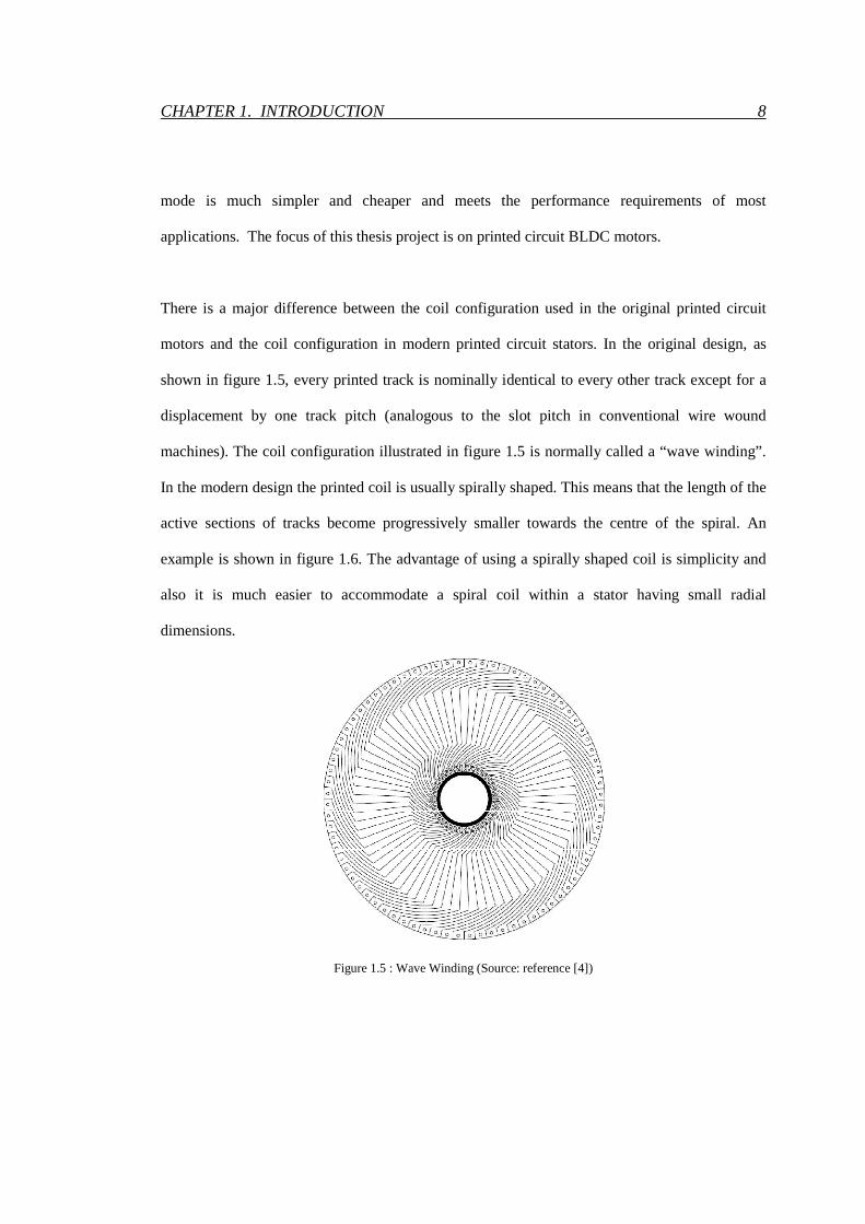
There is a major difference between the coil configuration used in the original printed circuit
motors and the coil configuration in modern printed circuit stators. In the original design, as
shown in figure 1.5, every printed track is nominally identical to every other track except for a
displacement by one track pitch (analogous to the slot pitch in conventional wire wound
machines). The coil configuration illustrated in figure 1.5 is normally called a “wave winding”.
In the modern design the printed coil is usually spirally shaped. This means that the length of the
active sections of tracks become progressively smaller towards the centre of the spiral. An
example is shown in figure 1.6. The advantage of using a spirally shaped coil is simplicity and
also it is much easier to accommodate a spiral coil within a stator having small radial
dimensions.
Figure 1.5 : Wave Winding (Source: reference [4])
CHAPTER 1. INTRODUCTION 9
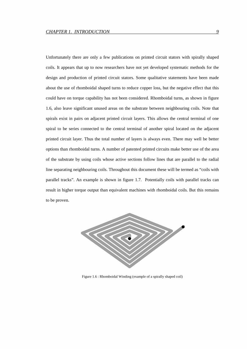
Unfortunately there are only a few publications on printed circuit stators with spirally shaped
coils. It appears that up to now researchers have not yet developed systematic methods for the
design and production of printed circuit stators. Some qualitative statements have been made
about the use of rhomboidal shaped turns to reduce copper loss, but the negative effect that this
could have on torque capability has not been considered. Rhomboidal turns, as shown in figure
1.6, also leave significant unused areas on the substrate between neighbouring coils. Note that
spirals exist in pairs on adjacent printed circuit layers. This allows the central terminal of one
spiral to be series connected to the central terminal of another spiral located on the adjacent
printed circuit layer. Thus the total number of layers is always even. There may well be better
options than rhomboidal turns. A number of patented printed circuits make better use of the area
of the substrate by using coils whose active sections follow lines that are parallel to the radial
line separating neighbouring coils. Throughout this document these will be termed as “coils with
parallel tracks”. An example is shown in figure 1.7. Potentially coils with parallel tracks can
result in higher torque output than equivalent machines with rhomboidal coils. But this remains
to be proven.
Figure 1.6 : Rhomboidal Winding (example of a spirally shaped coil)

CHAPTER 1. INTRODUCTION 10
Figure 1.7 : Coils with Parallel Active Sections
Based on elementary electromagnetic theory, it could be argued that the maximum torque from a
given length of track is obtained if that track runs along a radial line. This is the case because a
printed circuit machine being considered is an axial flux machine. That is the working or air-gap
flux is designed to be axial and motion of the rotor magnetic field relative to the stator tracks is
purely circumferential. Consequently maximum torque is obtained from current on the stator if it
flows in the radial direction, which is perpendicular to both the axial field and the direction of
relative motion of the rotor field. However, as shown in figure 1.8, the number of radial tracks is
heavily constrained by crowding near the inner radius of the substrate. Nevertheless, the radial
track option was not completely eliminated because it could represent the optimum choice under
special situations.

CHAPTER 1. INTRODUCTION 11
Figure 1.8 : Coils with Radial Active Sections
As mentioned in section 1.2, BLDC motors are normally three-phase machines. There are two
basic ways of implementing a three phase printed circuit stator. In the conceptually simpler
design, as exemplified in figure 1.9, a printed circuit layer belongs to one phase only. This
means that the total number of layers is a multiple of six. The layers belonging to one phase
would be identical to the layers belonging to the other two phases. However, as expected, the
magnetic axes of the coils of one phase will be shifted from the magnetic axes of the coils of the
other phases by 120 electrical degrees. The stator could be made up of a stack of three
substrates, as shown in figure 1.10, or a single substrate could be used for all phases. A feature
of this stator design is that the stator coil pitch is equal to the rotor pole pitch. This means that
the number of coils per layer is equal to the number of poles.

CHAPTER 1. INTRODUCTION 12
Figure 1.9 : Distribution of Coil on one Printed Circuit Layer (‘Four-Pole’ Flux Distribution)
Figure 1.10 : Exploded View of a Printed Circuit Axial Field Brushless Motor
Rotor Disks
Permanent Magnets
Y position [m]
0.01
0
-0.01
-0.02
-0.03
0.02 0
0.01
-0.01
-0.02
0
0.02
-0.02
Shaft Substrates
Z position [m]
X position [m]

CHAPTER 1. INTRODUCTION 13
The other way of implementing a printed circuit stator would be to have all three phases sharing
every printed layer. This means that the number of coils per layer must be a multiple of six. A
feature of this stator design is that the stator coil pitch is generally different from the rotor pole
pitch.
The following are some of the important variables that have to be considered in order to arrive at
an optimum printed stator design for a given application.
(a) Number of rotor poles
(b) Stator coil shape (wave wound, rhomboidal, radial or parallel)
(c) Nature of printed layers (each equally shared between phases or single phase per layer)
(d) Number of layers
(e) Track thickness
(f) Track width
(g) Track clearance
(h) Insulation material and insulation thickness
(i) Substrate material and substrate thickness
(j) Number of substrates that make up the stator stack
The task of making the correct decision with regards to the design variables listed above would
be greatly simplified if appropriate analytical and systematic design tools were available.
CHAPTER 1. INTRODUCTION 14
1.4 Sensorless Operation
Printed circuit brushless DC motors are relatively small motors and they are more likely to be
cost competitive if they can operate without position sensors. The back EMF zero crossing
method may be a good choice if good performance during starting and at low speeds are not
critical requirements. As back EMF is proportional to speed, the method does not work at and
near zero speed. Satisfactory sensorless operation at low speed and during start-up is possible
only by implementation of special techniques. One way of addressing the commutation problem
at start-up and at low speeds is to supplement the back EMF method with the “equal inductance
method” [2]. The latter method relies on the variation of stator inductance with rotor position.
This variation is characterised by the so-called saliency ratio of the machine. The method is
called the “equal inductance method” because detected positions of equal inductance of the
energised phase pair are used to determine the next commutation instant. While the equal
inductance method has been found to work with wire-wound motors having saliency ratios of
1.1 or more, it is not clear whether the method would work with printed circuit motors. The
significant differences between the characteristics of printed circuit machines and those of wire-
wound machines suggest that modifications of the originally proposed equal inductance method
would most likely be necessary for it to work with printed circuit motors.
Those, who at the motor design stage decide to use a sensorless method that is based on winding
inductance, must be able to make theoretical prediction of such inductance. Printed circuit
machine inductances are relatively easy to measure once the machine is built, but their

CHAPTER 1. INTRODUCTION 15
theoretical determination is not straightforward. The brute force approach to theoretical
determination of inductance would require detailed three dimensional non-linear electromagnetic
magnetic modelling under quasi static conditions. Typically such modelling would be carried out
using the finite element method. However, this approach does not suit many designers because
of lack of the necessary skills or computational resources. Also, due to the necessity for iterative
analysis to arrive at optimal designs, computer processing time may also be too long. There is a
need to develop sufficiently accurate but fast and computationally efficient techniques for
determining printed circuit motor self and mutual inductances.
1.5 Thesis Project Objectives
It is very likely that printed circuit motors will be used in an increasing number of modern
applications. However, there seems to be a lack of systematic design tools to assist printed
circuit motor designers. Also, to the author’s knowledge, there is no published work that
specifically addresses the question of sensorless operation of printed circuit BLDC motors down
to zero speed. The need to address those identified gaps has led to the following objectives for
this thesis project:
(a) to develop guidelines and a theoretical basis for the optimum electromagnetic design of
axial field printed circuit brushless DC motors;
(b) to experimentally validate the analytical techniques and design procedures that are
developed as part of this thesis project;

CHAPTER 1. INTRODUCTION 16
(c) to develop a position sensorless commutation method for axial field printed circuit
brushless DC motors that is effective down to zero speed;
(d) to experimentally validate the position sensorless commutation technique that is
developed as part of this thesis project and
(e) to develop a computationally efficient modelling technique that would allow prediction
of the self and mutual inductances of the phase windings of axial field printed circuit
brushless DC motors;
1.6 Outline of Dissertation
A review of the published works that are of relevance to the thesis project objectives is presented
in chapter 2. Details of the thesis project methodology and the reasoning behind it are given in
the same chapter.
Chapter 3 is devoted to the development of tools to help with the optimum design of printed
circuit board stators. These tools include computer algorithms for automatic stator track plotting
and phase EMF waveform prediction. The mathematical basis for the algorithms and their
experimental validation are also included.
Chapters 4 and 5 are about the enhancements made to and the generalisation of the originally
proposed equal inductance method. The enhancements reported in chapter 4 include a
commutation algorithm that incorporates a start-up technique which is also based on the equal

CHAPTER 1. INTRODUCTION 17
inductance method. Experimental results which validate the enhanced equal inductance method
are presented. The modified method, unlike the originally proposed method, does not require a
neutral connection.
The originally proposed equal inductance method assumes that the motor being controlled is
nominally symmetrical. Chapter 5 presents the mathematical arguments which were used to
arrive at a generalised equal inductance method applicable to the inherently asymmetric class of
printed circuit BLDC motors that was the focus of this thesis project. Experimental results which
confirm the validity of the generalised method are also presented.
Eddy currents induced within the stator tracks of printed circuit machines represent a parasitic
load and cause increased stator heating. In chapter 6 a mathematical model is proposed to
quantify stator eddy current loss. A specially designed laboratory test procedure is described
which has allowed predictions made by the model to be verified.
Chapter 7 presents fast and computer resource efficient mathematical algorithms that allow
stator winding inductances to be theoretically evaluated. Predictions made using the algorithms
have been experimentally verified. The computer algorithms can be used by designers, before
construction of physical prototypes, to check that sufficient inductive saliency is present for
successful application of the equal inductance method.
Conclusions of the thesis project are presented in chapter 8.

CHAPTER 1. INTRODUCTION 18
1.7 Main Outcomes of the Thesis Project
This thesis project has resulted in a number of useful outcomes for printed circuit board machine
designers. Analytical tools have been developed and validated to assist with optimisation of
printed stators. Designers will be able to maximise output torque while satisfying requirements
for maximum track width, minimum track width and inter-track clearance. In particular a
technique has been developed for quantitative assessment of eddy current losses within copper
tracks. Theoretical findings of the thesis project can be embedded into computer software for
quick assessment of the effect of changes in important design parameters such as stator
dimensions and pole numbers. It is also possible to use the developed design tools to explore
ways of reducing stator losses and improve efficiency without compromising torque capability.
While printed circuit motors may be operated in synchronous mode to achieve high performance
in terms of speed accuracy and torque quality, operating in brushless DC mode gives adequate
performance for most applications. A main advantage of the brushless DC mode is the
possibility of relatively simple sensorless implementation. Provided a brushless DC motor
exhibits enough saliency, very satisfactory performance at start-up and near zero speed is
possible if sensorless operation is based on the equal inductance method. The effectiveness of
the equal inductance method relies on the existence of sufficient saliency. An important
contribution from this thesis project is better understanding of the fundamental reasons behind
the existence of saliency in brushless printed circuit motors. This improved understanding has

CHAPTER 1. INTRODUCTION 19
led to a simplified electromagnetic model that allows saliency ratio and winding inductances to
be estimated by means of computationally efficient techniques.
An interesting point is that the equal inductance method was originally developed for nominally
symmetrical three phase machines. This thesis project dealt with an important class of printed
circuit machines which exhibits significant asymmetry. A significant outcome has been a
generalised equal inductance method that takes into consideration phase asymmetry.
The following journal papers, that have been published or accepted for publication, are direct
outcomes of this research project.
Ahfock A., Gambetta D., ‘Stator Eddy Current Losses in Printed Circuit Brushless DC Motors’,
Electric Power Applications, IET Proceedings, (accepted for publication)
Ahfock A., Gambetta D., ‘Sensorless Commutation of Printed Circuit Brushless DC Motors’,
Electric Power Applications, IET Proceedings, (accepted for publication)
Gambetta D., Ahfock A., ‘Design of Printed Circuit Brushless Motors’, Electric Power
Applications, IET Proceedings, Vol 3, Issue 5, Sept 2009, Pages 482-490

CHAPTER 1. INTRODUCTION 20
Gambetta D., Ahfock A., ‘A New Sensorless Commutation Technique for Brushless DC Motors’,
Electric Power Applications, IET Proceedings, Vol 3, Issue 1, Jan 2009, Pages 40-49

21
Chapter 2
Literature Review and Methodology
2
2.1 Literature Review
The purpose of the literature review was to find out about:
(a) any previously published work on design optimisation of printed circuit board motors;
(b) previously suggested techniques for low speed sensorless commutation control of
brushless motors that could be useful with axial field printed circuit BLDC motors;
(c) computational electromagnetic methods that could help with prediction of performance
of axial field printed circuit motors and
(d) computational electromagnetic methods that could help with the prediction of self and
mutual inductances of axial field printed circuit motors.

CHAPTER 2. LITERATURE REVIEW AND METHODOLOGY 22
2.1.1 Printed Circuit Motors
To date publications on printed circuit motors, such as references [6] to [10] have been limited
to:
(a) motors, with output torque of the order of a few milli-newtonmetres or less than 1 watt
per krpm, meant for applications such as computer drives and handheld video cameras;
(b) prediction of torque or back EMF for motors of predetermined coil configuration and
dimensions such as magnet thickness, rotor back-iron thickness and rotor-to-stator axial
length ratio.
In contrast, motors with power ratings up to tens of watts per krpm are being considered in this
thesis project. It seems that the requirement to keep axial thickness to a minimum has led
designers of axial field printed circuit to share printed circuit layers among all three phases. As
part of this thesis project, investigations will be carried out to find out whether this approach is
detrimental to electromagnetic torque production. There has been no rigorous analysis performed
to support the idea that rhomboidal coils represent the optimum coil configuration for axial flux
printed circuit motors. Systematic printed circuit board design algorithms will be developed as
part of this thesis project. These will allow the best coil configuration to be chosen for given
dimensional specifications of the motor space envelope.
Jang and Chang [6] use finite element analysis (FEA) to determine the axial force and torque for
a printed coil BLDC motor of given dimensions. They state that coils shaped as a wave winding
(figure 1.5) are not suited for stators with relatively small radii. They appear to use coils of

CHAPTER 2. LITERATURE REVIEW AND METHODOLOGY 23
concentric shape with radial or near radial active sections and with circumferential end sections.
No reasons are given for their choice of coil shape or their number of turns.
Tsai and Hsu [7] propose an analytical technique for prediction of air-gap flux density which is
verified by experiment and by using FEA. Their analytical method does not take into
consideration rotor back iron saturation and they do not specify if their three-dimensional FEA
does. They point out the better suitability of the rhomboidal printed coil for stators of low radii.
They also claim that the rhomboidal shape results in lower I2R loss. However, no quantitative
analysis is presented to support that claim. In particular there is no mention of whether the
benefit of lower I2R loss is gained at the expense of lower output torque capability.
Jang and Chang [8] present a relatively simple permeance model to predict the average airgap
flux density in axial field printed motors. The model is based on three permeance branches, one
for the axial path along the mechanical air-gap and printed coil, one for the axial path through
the magnet and one representing leakage paths. The calculated average air-gap flux density is
used to predict values for output torque for given coil currents. These compare well with
measured values. Details of any methodology used for designing the stator are not mentioned.
Low, Jabbar and Tan [9] describe a radial field printed circuit motor. Their focus is on the
elimination of cogging torque. They use a flexible PCB with concentric coils. The flexible PCB
is wrapped around a slotless laminated magnetic core to form an inner stator. Permanent
magnets are mounted on the inner surface of the outer hub. The reported electromagnetic design
procedure is essentially a one-dimensional representation which is based on assumed average
CHAPTER 2. LITERATURE REVIEW AND METHODOLOGY 24
values of flux density in the mechanical air-gap, printed circuit layers and iron cores. The one-
dimensional model is used to determine the required magnet thickness. There is no mention of a
systematic procedure aiming at design optimisation.
To the author’s knowledge there are no publications on a design procedure for axial flux printed
circuit motors where the electromagnetic design of the stator and that of the rotor are
simultaneously and systematically considered. In a typical application the space envelope for
the motor is usually specified in terms of a maximum radius and a maximum axial length. The
challenge for the designer is to produce a design that would meet torque output requirements and
that would fit in the specified envelope. The given axial length has to be shared between the
motor housing, the clearance between the motor housing and the rotor back-iron, the rotor back-
iron axial thickness (2ti), the permanent magnet axial thickness (2tm), the mechanical air-gap
axial length (2tag) and the stator axial thickness (ts). All the listed axial lengths may be
considered fixed except ti, tm, and ts. Since the total axial length is usually specified, the sum of
ti, tm, and ts would have to be equal to or smaller than a given value. This means that they cannot
be independently chosen. Takano, Ito, Mori, Sakuta and Hirasa [10] arrive at an optimum value
of 2 for tm/ ts for wire-wound machines. The existence of an optimum ratio is easily explained.
Torque is proportional to the product of the air-gap flux density set up by the permanent magnets
and the stator current. A relatively large value of tm would also require a relatively large value
of ti to avoid rotor back iron saturation. The choice of an excessively large value of tm leaves
very little room for a stator with reasonable current capacity and this leads to low torque rating.
On the other hand choosing an excessively large value of ts to boost current capacity leaves very
little room for the permanent magnets and the rotor back-iron. This leads to a weak air-gap flux

CHAPTER 2. LITERATURE REVIEW AND METHODOLOGY 25
density and low torque rating. There is clearly an optimal value of tm/ts . That optimum ratio
may be a function of other motor parameters. As part of this thesis project, generalised
algorithms will be developed to identify optimum tm/ts ratios for printed circuit axial field
motors.
For a given voltage rating, as the power rating of printed circuit stators increase, their printed
tracks would tend to be wider. For a fixed conductor thickness a wider track would not
necessarily mean a proportionately higher current carrying capacity since the track would also
suffer from increased circulating or eddy currents. The problem of eddy currents within stator
conductors of wire-wound machines has been previously analysed [11, 12]. However, to the
author’s knowledge, there is no publication on eddy currents induced in the conducting tracks of
a printed circuit stator.
Walker and Pullen [11] use a semi-empirical formula to determine eddy-current losses in a flat-
wire stator winding. Their method allows quick first estimation of eddy-current losses, but the
authors do not report experimental results nor do they comment on accuracy. Wang and Kamper
[12] use a combined numerical and analytical technique to solve a similar problem. The method
being proposed here is entirely numerical and avoids many of the simplifying assumptions made
in references [11] and [12]. For example no a priori assumptions are made about eddy current
paths and the entire winding is modelled, unlike reference [12] which does not consider the end-
winding.

CHAPTER 2. LITERATURE REVIEW AND METHODOLOGY 26
2.1.2 Sensorless Operation
It is advantageous to design printed circuit brushless motors so that they can be operated as
sensorless brushless DC motors. Sensorless position detection methods that have been proposed
to date for BLDC motors fall into two categories. There are those based on the use of back EMF
signals and those based on exploitation of inductive saliency. Back EMF based methods are only
applicable if speed is high enough. Nevertheless, there are many applications, for example drives
for fans or pumps, that do not require position control or closed-loop operation at low speeds.
For these, a back EMF based method is quite appropriate. Widely used, is the so called back
EMF “zero crossing” method, where the zero crossing instants of the un-energised phase are
used to estimate position [13]. It is important to mention that there is a 30° (electrical) offset
between the back EMF zero-crossing and the required commutation instant, which must be
compensated for to ensure correct operation of the motor [2,3].
BLDC motors which rely solely on back EMF signals for commutation suffer from relatively
poor starting performance characterised by initial back rotation of up to one hundred and eighty
electrical degrees and large fluctuations in electromagnetic torque resulting from non-ideal
commutation instants. This may not be acceptable for certain applications and there have been
attempts to develop sensorless techniques that give good performance right down to zero speed.
Most of those attempts, while being saliency based, have been aimed at the brushless
synchronous motor rather than the BLDC motor [14-20]. Saliency based sensorless techniques
for brushless synchronous motors are relatively complex because all the three phases are excited
one hundred percent of the time. They rely on measurement of current and voltage responses to
specially injected signals and require significant real time data processing. Ueki [21] and Weis
CHAPTER 2. LITERATURE REVIEW AND METHODOLOGY 27
[22] propose position detection techniques, based on saliency, specifically for BLDC motors and
they reduce complexity by exploiting the availability of an unexcited phase. But they also rely
on imposition of special signals onto the stator windings. Imposition of special signals requires
additional electronics, can cause additional heating and deterioration of torque quality.
In this thesis project a sensorless method of detection of commutation instants is proposed which
relies on inductive saliency. Unlike other proposed methods, no special signal injection is
needed. The computational burden to deduce commutation instants is negligible. The technique
is based on the detection of rotor positions where the two energised phases experience equal
inductances. It has therefore been termed the equal inductance method [2]. Gambetta [3]
required a neutral connection for practical implementation of the original version of the equal
inductance method. An objective of this thesis project is to modify the equal inductance method
so as to make the connection to the stator neutral unnecessary. The proposed refinement of the
original equal inductance method also incorporates initial position detection and start-up
algorithms. It is also envisaged that further adaptation of the equal inductance method will be
necessary. The originally proposed technique [2, 3] relies on the assumption that the BLDC
motor is symmetrical and that its phase winding electrical time constant, that is phase inductance
to phase resistance ratio, is relatively long compared the inverter pulse width modulation (PWM)
frequency. Both those assumptions are questionable in the case of axial field printed circuit
motors of the type shown in figure 1.9. The three phase windings of a symmetrical motor are
designed to have inductances that are equal except for a positional phase shift of 120 electrical
degrees. In the case of the printed circuit motor being considered the phase in the middle of the

CHAPTER 2. LITERATURE REVIEW AND METHODOLOGY 28
stator stack does not have the same inductance as the other two phases. Also the phase winding
time constant is relatively low because the stator is iron-less.
2.1.3 Measurement of Inductances and Inductive Saliency
When the equal inductance method is used, commutation positions are determined with a
resolution that is directly proportional the magnitude of the saliency ratio [2, 3]. Those planning
to use the method on existing machines can obtain the saliency ratio by measurement. In
addition to the saliency ratio, there may be a need for measurement of phase inductance to
ensure that the winding time constant is long enough compared to the inverter PWM period.
There exist numerous publications on measurement of saliency ratios and the inductances of
electrical machines [23-29]. However most of those relate to steady state performance of
synchronous or reluctance machines connected to the AC network. In those cases saliency ratios
or inductances are sought typically to allow determination of steady state performance under AC
conditions. The classical technique of measuring the saliency ratio of synchronous or reluctance
machines is the so-called slip test whereas the ‘synchronous’ inductance of synchronous
machines is measured by the short circuit test. All those previously published methods of
saliency measurement or synchronous inductance measurement are not applicable because the
inductances that are relevant to the equal inductance method are not “steady-state” inductances.
They are “transient” inductances in the same sense as the “transient reactance” used in
synchronous machine theory. Transient reactance (or inductance) is typically smaller than
synchronous reactance because it represents flux linkage for a phase winding which is mutually
coupled with other nearby shorted circuits. In the case of standard synchronous machines or

CHAPTER 2. LITERATURE REVIEW AND METHODOLOGY 29
reluctance machines, the windings to which the stator phase winding would be magnetically
linked are the field winding, damper windings and even eddy current loops within the solid steel
of the rotor. Ideally at steady state during balanced operation this coupling has no effect on
phase reactance because phase currents cause no induced currents in rotor circuits. This is the
case since under conditions of balanced stator currents and steady-state operation the rotating
magnetic field set up by the stator currents travel at the same speed as the rotor circuits. There
are no induced rotor currents to produce flux opposing the stator flux. Thus stator flux linkage
per ampere of stator current is highest. On the other hand rotor circuits play a role that could be
significant if the speed of magnetic fields set up by stator current is not equal to the rotor speed.
Such differences in speeds would occur as a result of unbalanced stator currents, harmonic
components in the stator current and stator current transients. In those cases flux linkage (and
therefore effective inductance) of a stator winding per ampere of stator current is reduced
because of the counter flux produced by induced currents in rotor circuit. The equal inductance
method involves sensing of voltage a relatively short time after switching events within the
inverter. Those switching events are occurring at the inverter PWM frequency. The reactance
experienced by stator currents resulting from those switching events would be influenced by
eddy currents induced within the body of magnets and within the solid rotor. Therefore the
relevant inductances are “transient” inductances. But the term “transient inductance” is a rather
loose term. In reality the value of such an inductance will be a minimum immediately after a
sudden change of stator voltage, when rotor opposing currents in rotor circuits are most
effective, to a maximum value after all currents in the rotor circuits have decayed to zero.
Reference [25] provides a clue to the question of which inductance value to use. It states that for
accurate results inductances must be measured under conditions approximating as closely as

CHAPTER 2. LITERATURE REVIEW AND METHODOLOGY 30
possible to those of normal operation. Based on this, it was assumed that inductances measured
with the rotor stationary and using sinusoidal currents at the inverter PWM frequency will be
those that are relevant to the equal inductance method. As part of this thesis project, laboratory
tests have been carried out to confirm the validity of this assumption. These tests consisted of a
comparison between absolute position determined by the equal inductance method which is itself
based on inductance values and those that are measured by a position sensor.
2.1.4 Prediction of Inductances and Inductive Saliency
Section 2.1.3 has focussed on measurement of saliency ratio or inductances that are applicable to
the equal inductance method. A related question is the prediction of those inductances at the
design stage of a brushless DC motor. Such information would be useful to those who intend to
use the equal inductance method but do not have access to the motor because it is yet to be
constructed.
As pointed out before the relevant transient inductances seem to be inductances experienced by
the stator sinusoidal phase current at relatively high frequency, typically a few tens of kilohertz.
A brute force approach to prediction of those inductances would be to use 3-D quasi-static finite
element analysis. However the computing and other resources to do this are not always
available. Long computation time could also be a problem, especially when multiple runs are
necessary to arrive at an optimal design. The difficulties in performing non-static three-
dimensional FEA on electrical machines are well documented [30-38].

CHAPTER 2. LITERATURE REVIEW AND METHODOLOGY 31
A computational electromagnetic method which is not as popular as FEA is the coupled network
method [39-51]. In its standard form, the method consists of a set of magnetic nodes and a set of
electric nodes. The nodes are located in 3-D space forming a regular pattern and are joined by
branches. The electric and magnetic nodes do not normally coincide. The magnetic branches are
reluctive and the electric branches are resistive. Loops formed by the magnetic branches link
loops formed by electric branches and vice-versa. Note that currents flowing in the electric
network may be induced or imposed. The branch reluctances and the branch resistances are
assumed to be known. The two networks are simultaneously analysed by a sets of node and/or
loop equations which are based on Maxwell’s Laws. An advantage of the coupled network
method is that it is amenable to physical interpretation [47, 48, 52]. Unfortunately, the coupled
network method, with no assumptions made about flux and current paths, is more restrictive than
the finite element method (FEM). The number of nodes required is generally more than the
number needed with FEM. It is a method that can be applied to simple geometries only.
Another version of the coupled network method is one based on assumed flux and current paths.
Again, in general two electromagnetically coupled networks are to be considered. But with this
method nodes do not have to be associated with regular spaced positions. The number of nodes
is normally greatly reduced compared to FEA or the coupled network method. The
magnetostatic version of the method is sometimes referred to as the permeance analysis method
or the magnetic flux tube method [36]. The main advantage of the assumed flux path method is
computational efficiency. However, the accuracy of the solution depends on the degree of
validity of the assumed flux and current paths.

CHAPTER 2. LITERATURE REVIEW AND METHODOLOGY 32
The adopted computational technique for the determination of inductance will be based on a
standard regular 2-D network of nodes and branches representing the magnetic field and a set of
assumed 1-D current paths making up the electric network. The two-dimensional approximation
of the magnetic field and the simplification of the current distribution to a set of one-dimensional
paths greatly improve computing efficiency. The physical reasoning behind the approximation
and simplification is presented. Tests have been carried out to validate the proposed technique of
inductance evaluation.
2.2 Methodology
The choice of thesis project methodology was influenced by the requirement to design cost
competitive BLDC motors with ratings in the range of tens of watts per krpm that:
(a) could be manufactured using standard modern printed circuit manufacturing processes;
(b) would fit in a space envelope defined by an axial length and a radius; and
(c) could be operated down to zero speed by means of a simple position sensorless
commutation technique such as the equal inductance method.
2.2.1 Design options and procedure
A number of choices exist for substrate and conducting materials for printed circuit boards.
Examples of substrate material are ceramic and FR4 (Flame Retardant 4). Examples of

CHAPTER 2. LITERATURE REVIEW AND METHODOLOGY 33
conducting material for the conducting track are silver and copper. It was quickly ascertained
during the early stages of the thesis project that FR4 substrates with copper tracks represented
the most practical and most economic option. FR4 copper clad laminate are widely available
commercially with a number of standard FR4 and copper thicknesses. Other relevant variables in
the manufacture of printed circuit boards are the number of printed circuit layers per substrate,
minimum track width, minimum clearance between tracks and track thickness. The cost of
manufacture depends non-linearly on the number of circuit layers. The cost of multi-layer
printed circuit boards escalates rapidly as the number of layers grows. It was found that beyond
eight to twelve layers per substrate the manufacturing costs of circuit boards become too
prohibitive for them to be used in motors. Consequently it was decided to keep the maximum
number of printed layers per substrate to eight. It was also decided to use standard commercial
track thicknesses to keep cost to a minimum. Minimum clearances used were those
recommended by FR4 laminate manufacturers. Those minimum clearances are a function of
copper track thickness. It should be noted that while decisions were made to use standard track
thicknesses, the design algorithm that was developed will allow the option of exploring non-
standard thicknesses.
Some investigations were carried out to help decide whether the printed coils on one layer
should belong to a single phase or whether they should be shared equally among three phases. It
was concluded that from the point of view of printed circuit board manufacturing it was much
simpler and cheaper not to have coils on a printed layer shared between phases. Another
advantage of having all coils of one layer belonging to just one phase is that, for a given total
stator axial thickness, torque per ampere is higher. Phase inductance variation from its q-axis

CHAPTER 2. LITERATURE REVIEW AND METHODOLOGY 34
value to its d-axis value is also closer to sinusoidal. Sinusoidal variation of inductance is an
important requirement of the equal inductance method which is planned to be used.
It was also decided to have one substrate per phase, as shown in figure 1.9. This allowed
designs with a larger number of layers per phase without exceeding the previously stated eight
layers per substrate.
Table 2.1 shows a list of the main design variables that had to be considered. These variables
have been divided into four groups. The first group, made up of the variables 1 to 5, are design
specifications. The assumptions are that they are fixed and that the objective is to arrive at a
design that achieves maximum output torque while respecting the constraints in Table 2.1.
The second set of variables, numbered 6 to 14, are essentially data that are associated with the
materials that have been selected by or provided to the designer for the manufacture of the motor
being designed. The design procedure is based on the assumption that those variables are fixed.
However, the designer may wish to go through the design procedure a number of times, each
time with one or more of those variables changed. For example, given the design specifications,
the design procedure could be separately used to arrive at the best design with different FR-4
laminates. This would allow the FR-4 laminate that gives the best design to be selected.
The third set of variables, that is the number of poles and the coil shape, are considered to be
outcomes of the design process. The planned design procedure will be such that, the number of
poles P and the coil shape will actually be input data to the procedure. However, if the most
suitable value of P was being sought, the procedure could be run a number of times to identify
that value of P. A similar statement can be made about the coil shape.

CHAPTER 2. LITERATURE REVIEW AND METHODOLOGY 35
The last group of variables, labelled 17 to 20 in Table 2.1, are outcomes of the planned design
procedure. The procedure is illustrated in figure 2.1. There are several iterative loops. Two of
those are shown explicitly. The determination of the minimum back iron thickness ti is
performed iteratively by changing ti and conducting non-linear 3-D magnetostatic analysis for
each value of ti. The search is for the minimum value of ti that results in the specified maximum
allowable flux density in the rotor back-iron. Note that the term ‘iteratively’ is being used to also
cover what is in essence a one-dimensional search for a value that satisfies a particular design
specification. For example tm is incremented from a minimum value and for each value the motor
torque capability is calculated. In this case the one dimensional search is for the value of tm that
results in maximum motor torque capability.

CHAPTER 2. LITERATURE REVIEW AND METHODOLOGY 36
Table 2.1 : Main Printed Circuit Motor Design Parameters
Design Parameter Degree of Flexibility
1 Outer Radius (Ro) Fixed specified value, dependent on intended application and
considered to be a design specification
2 Inner Radius (Ri) Fixed specified value, dependent on intended application and
considered to be a design specification
3 EMF (at 1000 rpm)
Fixed specified value together with tolerance, for example: 1V ±
10%. Considered to be a design specification that is dependent on
the intended application
4 Total axial length (ta) Fixed specified value, dependent on intended application and
considered to be a design specification
5 Stator/Magnet
Clearance(tc) Fixed specified value, typically 0.3 mm
6 FR4 insulation layer
thickness
Fixed specified value obtained from data sheet of chosen FR4 /
Cu laminate
7 Track thickness Fixed specified value obtained from data sheet of chosen FR4 /
Cu laminate
8 Clearance between
tracks
Fixed specified value obtained from data sheet of chosen FR4 /
Cu laminate
9 Minimum track width Fixed specified value obtained from data sheet of chosen FR4 /
Cu laminate
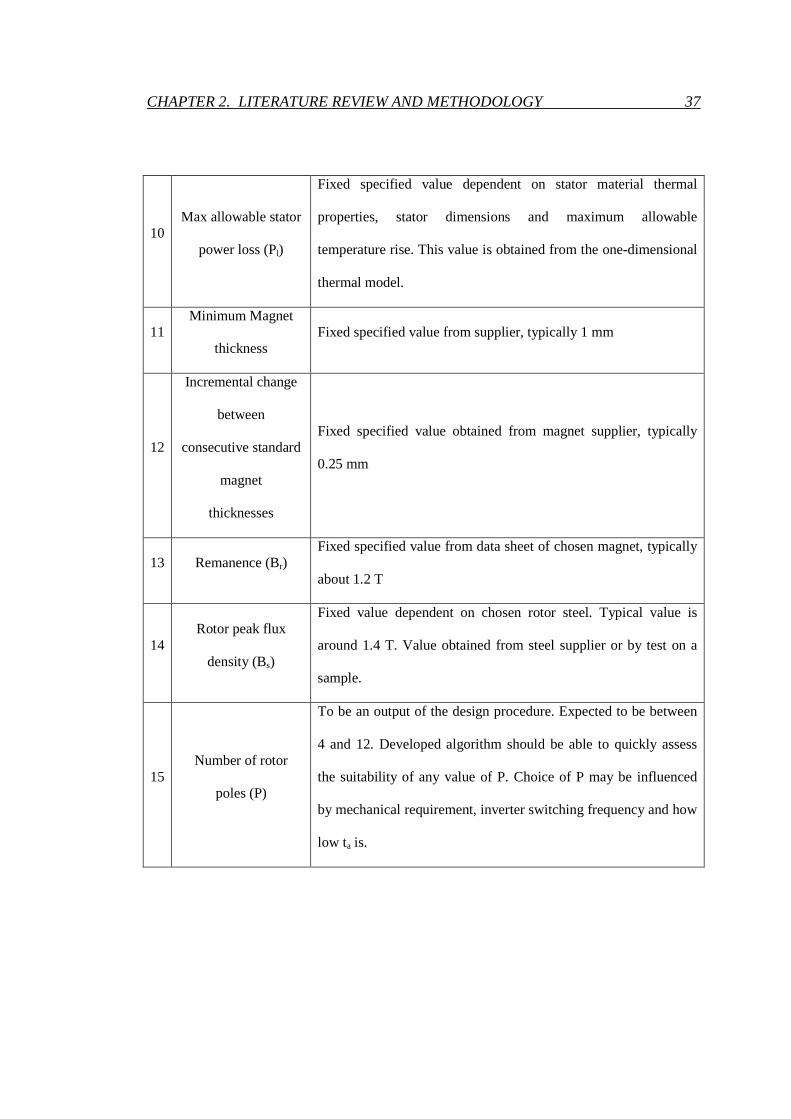
CHAPTER 2. LITERATURE REVIEW AND METHODOLOGY 37
10 Max allowable stator
power loss (Pl)
Fixed specified value dependent on stator material thermal
properties, stator dimensions and maximum allowable
temperature rise. This value is obtained from the one-dimensional
thermal model.
11 Minimum Magnet
thickness Fixed specified value from supplier, typically 1 mm
12
Incremental change
between
consecutive standard
magnet
thicknesses
Fixed specified value obtained from magnet supplier, typically
0.25 mm
13 Remanence (Br) Fixed specified value from data sheet of chosen magnet, typically
about 1.2 T
14 Rotor peak flux
density (Bs)
Fixed value dependent on chosen rotor steel. Typical value is
around 1.4 T. Value obtained from steel supplier or by test on a
sample.
15 Number of rotor
poles (P)
To be an output of the design procedure. Expected to be between
4 and 12. Developed algorithm should be able to quickly assess
the suitability of any value of P. Choice of P may be influenced
by mechanical requirement, inverter switching frequency and how
low ta is.

CHAPTER 2. LITERATURE REVIEW AND METHODOLOGY 38
16 Coil shape
To be an output of the design procedure. For dimensions of Ro
and Ri normally under consideration, the best coil shape will most
likely have parallel active sections or mixed parallel and radial
sections.
17 Rotor Iron thickness
(ti)
To be an output of the design procedure, but should be greater
than 1 mm to ensure adequate mechanical strength.
18 Magnet thickness
(tm)
To be an output of the design procedure. However only discrete
values above a minimum is allowed. The discrete values and the
minimum value depend on the chosen supplier.
19 Number of turns per
coil (N) To be an output of the design procedure
20
Number of printed
circuit
layers per phase (L)
To be an output of the design procedure

CHAPTER 2. LITERATURE REVIEW AND METHODOLOGY 39
Figure 2.1 : Generalised Printed Circuit Motor Design Optimisation Flow-chart

CHAPTER 2. LITERATURE REVIEW AND METHODOLOGY 40
Inspection of table 2.1 and figure 2.1 reveals that a number of tools are to be developed to
implement the design optimisation procedure. These are:
(a) A 1-D thermal model to calculate, using material data, the maximum allowable stator
power loss;
(b) A technique for the measurement of the magnetising curve of samples of the steel that is
used for the rotor;
(c) Computer algorithms to automatically plot coil tracks;
(d) Computer algorithms to automatically determine phase EMF waveforms;
(e) A mathematical model to predict eddy current loss in stator copper tracks. There is a
need to ensure that stator tracks are below the width that would cause excessive eddy
currents.
Prototypes will be specially designed to validate theoretical predictions made in (d) and (e)
above.
2.2.2 Modification and adaptation of the equal inductance method
Theoretical results and encouraging practical performance data reported in reference [2] were
behind the decision to focus on the equal inductance method as the sensorless technique for the
printed circuit motors being developed as part of this thesis project. As stated before the
originally reported equal inductance method needed a connection to the neutral point of the star-
connected stator. Also there were no reported starting performance data and the method had not

CHAPTER 2. LITERATURE REVIEW AND METHODOLOGY 41
been tried with motors with low phase inductance. The plan was to further develop the equal
inductance method so that it does not need a neutral connection and to adapt it so that it is
compatible with the ironless printed circuit axial field machines. Since the equal inductance
method cannot work successfully without a minimum level of saliency there is a need for a
mathematical procedure to predict inductance and saliency at the design stage.
Considering the points presented in the preceding paragraph the following were planned:
(a) Theoretical analysis to confirm that the equal inductance method, if suitably modified,
will work without a neutral connection;
(b) Confirmation, by laboratory tests performed on standard radial field wire-wound
motors, that the modified equal inductance method performs well both at steady state
and during starting;
(c) Measurement of the inductance and mutual inductance characteristics of printed circuit
machines such as the one illustrated in figure 1.9 to ascertain the nature of further
modifications that would be necessary to adapt the equal inductance method to suit those
motors;
(d) Development of the necessary further modification of the equal inductance method to
make it suitable to printed circuit motors. This would be based on theoretical analysis.
(e) Assessment of performance of the adapted equal inductance method by carrying out
laboratory tests on printed circuit motors. The assessment is to cover both steady-state
commutation performance and start-up performance.

CHAPTER 2. LITERATURE REVIEW AND METHODOLOGY 42
(f) Development of an efficient computational method to determine d-axis and q-axis self
and mutual inductance of the phase windings of printed circuit motors such as the one
illustrated in figure 1.9. Analysis will be based on a coupled network made up of a 2-D
permeance network coupled with assumed current paths in the form of discrete loops.

43
Chapter 3
Printed Circuit Stators for Brushless
Permanent Magnet Motors
3
3.1 Introduction
While the first printed circuit armatures used brushes and mechanical commutation,
developments in power electronic devices and control systems have led to printed circuit motors
that are brushless. Modern cost effective neodymium magnets have allowed compact motor
designs. Multi-layer circuit board production techniques have made the production of printed
circuit coils cheaper and easier. However, in spite of the growing importance of printed circuit
brushless motors, there is a lack of analytical tools to assist with their design. This chapter uses
geometrical analysis to arrive at general mathematical expressions which allow the plotting of

CHAPTER 3. PRINTED CIRCUIT STATORS FOR BRUSHLESS PM MOTORS 44
printed circuit tracks to be carried out more systematically. Track plotting procedures have been
developed for four different coil shapes.
These are spirals with purely radial active sections, spirals with active sections running parallel
with each other, spirals with each active section having a radial part and a parallel part and
rhomboidal shaped spirals. For each spiral shape, equations are derived for the maximum
number of turns (N). The maximum number of turns is generally a function of the substrate inner
radius (Ri), the substrate outer radius (Ro), the track minimum width (w) and the minimum
clearance between tracks (c). To produce the printed stators, the tracks are plotted with the help
of algorithms that maximizes the effectiveness of the coil. Appropriate measures of coil
effectiveness are the EMF constant or the torque constant of the coil and the total resistance of
the coil. Theoretical predictions of EMF constants and EMF waveforms are presented in section
3.3. The predictions are based on realistic flux distributions obtained from finite element
analysis. Extensive tests on six prototype motors were carried out to validate the theory on which
the proposed design techniques are based. A comparison between theoretical predictions and test
results are presented in section 3.4. A general design algorithm based on the track plotting
procedure and the EMF prediction technique is presented in section 3.5.

CHAPTER 3. PRINTED CIRCUIT STATORS FOR BRUSHLESS PM MOTORS 45
3.2 Analysis of Coil Geometries
Consider a section of the substrate as shown in figure 3.1. The simplest coil is made up of a
spiral pair. The two spirals making up a pair are located on adjacent layers of the PCB or on
opposite side of the substrate if there are only two layers. The spirals are joined by a via located
at their common centre. In figure 3.1, the two spirals making up a pair are the “top layer spiral”
and the “bottom layer spiral”. Current enters the coil from a terminal on the outer radius side of
the substrate. It flows inwards, towards the coil center, through the tracks of one of the spirals,
continues through the via at the centre of the spiral and then flows outwards, away from the coil
center, through the tracks of the second spiral. The directions of current in the two spirals are
such that the torque produced by one spiral is equal and adds to the torque produced by the
second spiral. Similarly, the rotational EMF generated in one spiral is equal and adds to the EMF
generated in the other spiral.

CHAPTER 3. PRINTED CIRCUIT STATORS FOR BRUSHLESS PM MOTORS 46
a)
b)
Figure 3.1 : (a) Top Layer Spiral (b) Bottom Layer Spiral

CHAPTER 3. PRINTED CIRCUIT STATORS FOR BRUSHLESS PM MOTORS 47
In general each turn of a coil may be considered to be made up of four sections. Two of those are
non-active arc-shaped end-sections, one on the outer radius side and one on the inner radius side.
The other two sections are active. The length of some of the arc-shaped inner end-sections may
degenerate to zero for low values of Ri/Ro. To maximize the effectiveness of a coil its number of
turns, average active length per turn and overall pitch factor must be maximized. Assuming the
air-gap flux is purely axial, the maximum EMF per unit length is obtained if the active conductor
runs along a radial line. However, the number of turns can be adversely affected if Ri/Ro is small
and the active sections are constrained to be radial. Parallel active sections are preferable
although this leads to longer inactive sections. Coils with active sections which are partly
parallel and partly radial are investigated because they offer the possibility of reduced total
conductor length while maintaining performance in terms of EMF per unit speed or torque per
unit current. Expressions are now derived for the maximum number of turns.
3.2.1 Purely Parallel Coils
In figure 3.2 (a) point X is at the centre of the coil and lies somewhere along the radial line
which is the axis of symmetry of the coil. Proper placement of point X is required if a coil with
maximum number of turns (N) is to be achieved. In general for given values of minimum track
width (w) and minimum inter-track clearance (c), the number of turns is limited by (Ro-Rx) or
XP or (Rx-Ri). If X is placed too far towards the outer edge of the substrate, N is reduced
because it becomes restricted by the smaller value of (Ro-Rx). Similarly, if X is placed too far
towards the inner edge of the substrate, N is again reduced because it becomes restricted either
by the smaller value of XP or by the smaller value of (Rx-Ri).

CHAPTER 3. PRINTED CIRCUIT STATORS FOR BRUSHLESS PM MOTORS 48
P
X
Rx Ro
Ri
sN
π
Figure 3.2(a) : Half Spiral Section of Substrate
Figure 3.2(b) : Example of Printed Coil with Parallel Tracks
-0.025 -0.02 -0.015 -0.01 -0.005 0 0.005 0.01 0.015 0.02 0.0250
0.005
0.01
0.015
0.02
0.025
X position [m]
Y p
ositi
on [
m]
Track middle lineRadial position reference linesAngular position reference lines

CHAPTER 3. PRINTED CIRCUIT STATORS FOR BRUSHLESS PM MOTORS 49
Based on the preceding arguments, it can be concluded that there is a position for X that results
in the maximum number of turns. For small values of Ri/Ro, the number of turns is maximized if:
( )
=−
sxxo N
RRRπ
sin (3.1)
where Ns= number of spirals per layer
For larger values of Ri/Ro, the number of turns is maximized if:
( ) ( )ixxo RRRR −=− (3.2)
That is the optimum value of Rx is ( )
2o iR R+
From equation (3.1) it can be deduced that:
( )
++
=
s
so
Ncw
NR
Nπ
π
sin1
sin
(3.3)
Equation (3.3) is applicable if:
+
−
≤
s
s
o
i
N
N
R
R
π
π
sin1
sin1
(3.4)
From equation (3.2) it can be deduced that:
( )( )cw
RRN io
+−
=2
(3.5)
Equation (3.5) if valid if:

CHAPTER 3. PRINTED CIRCUIT STATORS FOR BRUSHLESS PM MOTORS 50
+
−
≥
s
s
o
i
N
N
R
R
π
π
sin1
sin1
(3.6)
Equation (3.3) and inequality (3.4) represent a circumferentially restricted coil whereas equation
(3.5) and inequality (3.6) represent a radially restricted coil.
For a prescribed track width, equation (3.3) or (3.5) is to be used to determine N which has to be
an integer. The equation can then be used again, with N fixed at its integer value, to readjust the
track width to a higher value.
An example of a printed coil with parallel tracks is shown in figure 3.2(b).
3.2.2 Purely Radial Coils
Purely radial spirally wound coils are unlikely to be adopted by designers except possibly for
cases where both Ri/Ro and Ns are high. Based upon arguments similar to those presented in
section 3.2.1, it can be deduced that for large enough values of Ri/Ro:
( )( )cw
RRN io
+−
=2
(3.7)
With the help of figure 3.3 (a), an expression can be derived for cases where values of Ri/Ro are
low. In order for N to be a maximum equation (3.8) must be satisfied.
( )cw
rddn
+= θ
, for sN
πθ ≤≤0 (3.8)

CHAPTER 3. PRINTED CIRCUIT STATORS FOR BRUSHLESS PM MOTORS 51
where n= number of turns counting from the inter-coil boundary line
and ( )cwnRr i ++=
P
X
Ro
Ri
rθ
d
d
d=w+c
Figure 3.3(a) : Radial Tracks (d exaggerated for clarity)
Figure 3.3(b) : Example of Printed Coil with Radial Tracks
-0.025 -0.02 -0.015 -0.01 -0.005 0 0.005 0.01 0.015 0.02 0.0250
0.005
0.01
0.015
0.02
0.025
X position [m]
Y p
ositi
on [
m]
Track middle lineRadial position reference linesAngular position reference lines

CHAPTER 3. PRINTED CIRCUIT STATORS FOR BRUSHLESS PM MOTORS 52
Integration of both sides of equation (3.8) from 0=θ to sN
πθ = leads to:
( )cw
eR
N
sNi
+
−
=
1π
(3.9)
Equation (3.7) is applicable if:
−
≥
12
1
sNo
i
eR
Rπ (3.10)
Equation (3.9) is applicable for smaller values of Ri/Ro. Inequality (3.10) is arrived at by
equating the right hand side of equations (3.9) and (3.7).
An example of a printed coil with purely radial tracks is shown in figure 3.3(b). The above
equations were used to confirm that, with Ri/Ro ratios considered in this thesis project, purely
radial coils represent significantly inferior designs compared with coils with parallel or mixed
parallel and radial sections. Therefore purely radial coils are not given further consideration.
3.2.3 Mixed Parallel and Radial Track Sections
An example of a spiral coil with mixed track sections is shown in figure 3.4. Only the mid-track
line is shown.

CHAPTER 3. PRINTED CIRCUIT STATORS FOR BRUSHLESS PM MOTORS 53
Figure 3.4 : Mixed Track (showing reference lines used for EMF evaluation)
A strategy has been adopted that maximizes the lengths of radial sections of the track subject to
meeting minimum clearance requirements between tracks. This is achieved by keeping the track
sections parallel on the inner radius side of arc XQ whose radius is defined by equations (3.1) or
(3.2). Radius Rx is defined in exactly the same way as in section 3.2.1. Arc XQ is shown in
figure 3.5. On the outer side of arc XQ, track sections are radial. The positions of all track
sections are fully defined if Ri, Ro, w and c are known. The adopted algorithm to produce the
tracks starts with the positioning of the inner arc sections and the parallel sections. The inner
end-points of the radial sections are then known since they are where the parallel sections meet
arc XQ. The radial sections can then be positioned since they lie on straight lines defined by the
centre of the circle and the points where the parallel sections meet arc XQ.
-0.025 -0.02 -0.015 -0.01 -0.005 0 0.005 0.01 0.015 0.02 0.0250
0.005
0.01
0.015
0.02
0.025
X position [m]
Y p
ositi
on [
m]
Track middle lineRadial position reference linesAngular position reference lines

CHAPTER 3. PRINTED CIRCUIT STATORS FOR BRUSHLESS PM MOTORS 54
P
X
Rx Ro
Ri
sN
π
d=w+c
Q
d
d2
d
2
d
2
d
Figure 3.5 : Section of Substrate (Mixed Track Sections)
3.3 Predicting Coil EMF’s
Back EMF per phase is an important measure of performance for a motor. The back EMF
waveform allows deduction of the motor’s torque capability and its torque quality. Prediction of
back EMF waveforms requires knowledge of the flux density distribution. Depending on the
level of accuracy required, this can be determined analytically or numerically. The machines
being considered in this thesis project have relatively complex coil and magnetic circuit
geometries and parts of the rotor iron may saturate magnetically. Consequently it is not possible
to arrive at analytical expressions that will allow prediction of rotational EMF with better than

CHAPTER 3. PRINTED CIRCUIT STATORS FOR BRUSHLESS PM MOTORS 55
ten per-cent accuracy. Therefore there is a need to rely on numerical methods. The adopted
numerical techniques are presented in section 3.3.2.
In spite of its limited accuracy, an analytical technique can be valuable to those who have to
shortlist design configurations that deserve detailed analysis. An equation is suggested in section
3.3.1 that can be used to evaluate the rotational EMF to a first approximation. In both sections
3.3.1 and 3.3.2 it has been assumed that the number of rotor poles (P) is equal to the number of
spirals (Ns) per printed circuit layer. It is possible to construct three phase motors with Ns not
equal to P, but such motors are not considered in this work. Every stator under consideration was
made up of three sets of printed layers circumferentially displaced from each other by 120
electrical degrees. This results in a small degree of asymmetry since the phase that is sandwiched
between the other two has a slightly lower EMF. Theoretical and experimental results that are to
be presented have allowed the practical significance of this asymmetry to be assessed.
An exploded view of one of the prototype motors is given in figure 3.6. All motors that were
constructed are of the central stator dual rotor type. The single rotor option was not chosen
because:
(a) A laminated back iron disk will be needed on which to mount the printed circuit boards.
(b) There would be increased asymmetry.
(c) Without the magnet, the relative amount of leakage flux will increase.

CHAPTER 3. PRINTED CIRCUIT STATORS FOR BRUSHLESS PM MOTORS 56
Figure 3.6 : Exploded View of one of six Test Motors
3.3.1 Approximate Analytical Modelling
The major simplifying assumptions that had to be made to arrive at an analytical expression for
rotational EMF are:
(a) active track sections are in the radial directions and their lengths change linearly with
angular position from (Ro-Ri) at the coil’s edge to zero at its centre;
Rotor disks
Permanent Magnets
Y position [m]
0.01
0
-0.01
-0.02
-0.03
0.02
0
0.01
0.02
-0.01
-0.02
0
0.02
-0.02
Shaft Substrates
Z position [m]
X position [m]

CHAPTER 3. PRINTED CIRCUIT STATORS FOR BRUSHLESS PM MOTORS 57
(b) the rotor iron has infinite permeability;
(c) flux outside the rotor iron flows in the axial direction only;
(d) flux density in the airgap is independent of radial and axial positions;
Equation (11) is based on the above assumptions.
( )( )2
2 cmpkioio SBRRRRNPE
ω−+= (3.11)
where:
E = EMF per spiral
mω = rotational speed
N = number of turns per spiral.
P = number of poles.
Bpk = airgap peak flux density =
+2g
t
tB
m
mr (3.12)
Br = remanence of permanent magnet.
tm = magnet thickness
g = airgap length measured axially between opposite magnet surfaces
Sc = combined length, spread and pitch factors of coil
=2
2
0
4cos
21
2
πθθ
πθ
π
π
=
−∫ d
θ = electrical angle

CHAPTER 3. PRINTED CIRCUIT STATORS FOR BRUSHLESS PM MOTORS 58
Equation (3.12) has been derived using a 1-D magnetic model. Details on that model can be
found in Appendix A. The 1-D model is based on the assumptions that:
a) Iron Permeability = infinity
b) Permanent Magnet Permeability = µ0 = 1
It has been assumed that the airgap flux density varies sinusoidally in the angular direction. This
is a reasonable assumption because the effect of higher harmonics is significantly reduced as a
result of the coils being distributed and short-pitched.
An approximate technique for determination of axial dimensions can be based on equations
(3.13) and (3.14).
ti = axial thickness of rotor = s
iompk
PB
RRSB
2
)( +π (3.13)
where:
Bs = maximum allowable flux density in the rotor iron
Sm = pitch factor magnet
ta = total axial length = ( )2 3i ag m st t t t+ + + (3.14)
where:
ts = stator thickness per phase.
tag = clearance between magnet surface and stator surface

CHAPTER 3. PRINTED CIRCUIT STATORS FOR BRUSHLESS PM MOTORS 59
3.3.2 Predicting Coil EMFs Numerically
This section provides details of a numerical solution to the problem of predicting the phase EMF
waveforms. For the purpose of determining motional induced EMF, the plane of the substrate is
divided into cells as shown in figure 3.4. Each cell is bounded by a pair of radial reference lines
and a pair of angular reference lines. The total EMF corresponding to a given rotor position is
generally made up of contributions coming from each cell. The number of active track segments
within a cell may be zero, one or two. Contributions to the total EMF are separately calculated
for each segment by using equation (3.15).
rdrBdE mω*= (3.15)
where:
dE = contribution to total EMF from each track segment
B* = estimated flux density at point C in figure 3.7
r = radial distance as shown in figure 3.7
dr = (ro-ri) as shown in figure 3.7
mω = rotational speed

CHAPTER 3. PRINTED CIRCUIT STATORS FOR BRUSHLESS PM MOTORS 60
1
rl
2
4 3
rs
ro
ri
r
C
aθbθ
Figure 3.7 : Track Segment in a Cell (segment centred at point C)
The estimated value (B*) of flux density is obtained by using:
lirirolo wwBwwBwwBwwBB 4321* +++= (3.16)
where:
( )( )sl
so rr
rrw
−−=
( )( )sl
li rr
rrw
−−=
( )ba
blw
θθθ+
=
( )ba
arw
θθθ+
=

CHAPTER 3. PRINTED CIRCUIT STATORS FOR BRUSHLESS PM MOTORS 61
It is assumed that the flux density at the four corners of every cell (B1-B4 in figure 3.7) is
known. In general flux density (B) is a function of all spatial coordinates. Variation in the axial
direction does not have to be considered since, for the purpose of coil EMF evaluation, it is
reasonable to assume that all track segments making up a coil are at the same axial position. Flux
distributions were obtained from finite element analysis. This has been done for a number of
configurations with different values of P, Ro and Ri.
As shown in figure 3.8, finite element modeling was carried out using FEMLAB®.
Motors from 4 to 12 poles with dual rotor and central stator construction were considered.
Existence of axial and circumferential symmetry meant that only half a pole pitch of one rotor
had to be modeled. Figure 3.8 shows the model for a four pole motor.
Figure 3.8 : FEMLAB® Model of the Rotor (Half Pole Pitch)
Y position [m]
Z position [m]
X position [m] 0
0.01 0.02
0.03 0.04
0.05 0
0.01
0.02
0.03
0 0.01
0.02 0.03

CHAPTER 3. PRINTED CIRCUIT STATORS FOR BRUSHLESS PM MOTORS 62
A plane of symmetry exists at z = 32.7 mm. The axial flux density distribution on that plane is
used to evaluate the EMF of the middle phase. There is no need for explicit modeling of the
stator since all the materials making up the stator are assumed to have relative permeability
equal to one and no stator current flows. In addition to the air subdomain whose relative
permeability is taken to be one, there are three other subdomains that have been considered.
These are the permanent magnet subdomain which in figure 7 is between z = 26 mm and z = 30
mm, the rotor back-iron subdomain which is between z = 22 mm and z = 26 mm and the sub-
domain representing the non-magnetic shaft. Based on the manufacturer’s data, a value of 1.01e6
H/m was used for the magnetization of the NdFeB permanent magnet.
The rotor back-iron has been characterized by its magnetization curve which was determined
experimentally since no reliable data were available. Measurement has been carried out on ring
core shaped samples. A 50 Hz sinusoidal current (increased stepwise) was injected in the
‘primary’ winding. This current is directly proportional to magnetic strength H. Due to the
imposed current a voltage v(t) is induced. Since:
( ) mdv t
dt
ψ= − (3.17)
with mψ = flux through the core cross-sectional area, the flux density B is:
( )
core
v t dtB
A= ∫ (3.18)
For every current level a B-H loop was generated, as shown in figure 3.9. To compute the
relative iron permeability, the maxima values of B and H were used. These values are
represented by the dots in figure 3.9.

CHAPTER 3. PRINTED CIRCUIT STATORS FOR BRUSHLESS PM MOTORS 63
-1.5 -1 -0.5 0 0.5 1 1.5
x 105
-2.5
-2
-1.5
-1
-0.5
0
0.5
1
1.5
2
2.5
Magnetic Strength H [At/m]
Mag
netic
Flu
x D
ensi
ty [
T]
Figure 3.9 : B-H Loops of Rotor Material
The relative permeability of the shaft was taken as one. A typical axial flux density distribution
obtained from finite element results is shown in figure 3.10.
As the rotor moves the flux distribution shown in figure 3.10 rotates relative to the radial
reference lines shown in figure 3.4. As part of the algorithm that determines the rotational EMF
waveform, the rotor position is changed in incremental steps and for each step a phase EMF
value is calculated based on equation (3.15). A set of EMF values corresponding to one
electrical cycle represents an EMF waveform. EMF waveforms for different phases are
calculated using axial flux densities at the axial location of that phase.

CHAPTER 3. PRINTED CIRCUIT STATORS FOR BRUSHLESS PM MOTORS 64
Figure 3.10 : Output from Finite Element Analysis (Axial Flux Density)
Before introducing the experimental results (section 3.4), some considerations on rhomboidal
shaped spirals will follow. As expected the rhomboidal geometry presents lower resistance and
lower EMF than the mixed track sections or the parallel track section designs. A comparison
based on the torque capability factor R
PE l
m
ω(explained in section 3.4), clearly shows that the
rhomboidal approach does not perform as well as the other two. The resulting difference is about
10%. Different rhomboidal shapes have been analyzed, two of them are presented in figures 3.11
and 3.12.
0pi/2
pi3/2*pi
2*pi
00.005
0.010.015
0.020.025
0.03-1
-0.5
0
0.5
1
Rotor Position Θ [electrical radian]
Arc-length [m]
Mag
netic
flu
x de
nsity
[T
]

CHAPTER 3. PRINTED CIRCUIT STATORS FOR BRUSHLESS PM MOTORS 65
-0.02 -0.015 -0.01 -0.005 0 0.005 0.01 0.015 0.020
0.005
0.01
0.015
0.02
0.025
[mm]
[mm
]
Figure 3.11 : “B” Point “max shift” in Direction Outer Radius
-0.02 -0.015 -0.01 -0.005 0 0.005 0.01 0.015 0.020
0.005
0.01
0.015
0.02
0.025
[mm]
[mm
]
Figure 3.12 : “B” Point in Intermediate Position between Outer and Inner Radius
CHAPTER 3. PRINTED CIRCUIT STATORS FOR BRUSHLESS PM MOTORS 66
The best performing “rhomboidal” design, from a point of view of EMF is the one where the
position of the B points (vertices) is maximized (maximal shift toward the outer radius). This
particular B point configuration also results in near to sinusoidal EMF waveform. If the B points
are shifted towards the inner radius the waveform gets quite distorted.
3.4 Experimental Verifications
Six motors were built to validate the coil design and EMF prediction procedures that have been
proposed. Details of the motors are given in table 3.1. All motors have an outer radius of 25 mm,
a rotor iron thickness of 4 mm, a magnet thickness of 4mm, a nominal track width of 1 mm and a
track clearance of 0.3 mm. The outer dimensions were made equal to those of an existing
commercial motor so that meaningful performance comparison could be made.
3.4.1 EMF Waveforms
A set of EMF waveforms for one of the prototype motors is shown in figure 3.13. For all six test
motors, there is very good agreement between the predicted and measured waveforms. RMS
values of the waveforms are given in table 3.1.

CHAPTER 3. PRINTED CIRCUIT STATORS FOR BRUSHLESS PM MOTORS 67
Figure 3.13 : Phase EMF Waveforms (Test Motor No. 1, 1000 r/min)
The sine wave approximation for the EMF waveform is well-justified since the total harmonic
distortion is less than 2%.
0 5 10 15 20 25 30
-1
-0.5
0
0.5
1
Time [ms]
EM
F [
V]
Simulated EMFA
Simulated EMFB
Simulated EMFC
Measured EMFA
Measured EMFB
Measured EMFC

CHAPTER 3. PRINTED CIRCUIT STATORS FOR BRUSHLESS PM MOTORS 68
Table 3.1 : Motor Test Data
o
i
R
R
P
Track
Type N Bpeak [T]
E [Vrms]
R [Ω] R
PE l
m
ω [mNm]
(pred.)
(eq. 3.11)
(pred.)
FEM (meas.) (pred.) (meas.) (meas.)
1 0.20 4 Parallel 7 0.708
0.757
0.816 0.846 0.092 0.092 40.3
2 0.20 4 Mixed 7 0.708 0.810 0.840 0.085 0.084 42.0
3 0.36 4 Parallel 6 0.702
0.597
0.675 0.689 0.087 0.086 34.0
4 0.36 4 Mixed 6 0.702 0.672 0.687 0.084 0.083 34.5
5 0.20 8 Parallel 5 0.655
0.965
0.987 1.000 0.093 0.095 47.0
6 0.20 8 Mixed 5 0.655 0.975 0.987 0.090 0.091 47.4

CHAPTER 3. PRINTED CIRCUIT STATORS FOR BRUSHLESS PM MOTORS 69
As expected, the EMF waveform of the middle phase within the stator stack has slightly lower
magnitude than the outer phases. The difference is typically less than 3.5% and does not
represent any significant problem to motor performance. EMF predictions by the first order
model in section 3.3.1 are within ten percent of those based on finite element.
3.4.2 Thermal Considerations
Both from the point of view of stator temperature rise and from the point of view of efficiency a
reduction of printed circuit coil resistance is desirable. However a reduction in phase resistance
should not be at the expense of an excessive reduction in EMF. An objective assessment of
different strategies to reduce phase resistance may be based on the value of R
PE l
m
ωwhere Pl is
the allowable stator power loss per phase. The term R
PE l
m
ω is proportional to the torque
capability of the motor. The constant of proportionality depends on the shape of the phase
current which would be sinusoidal for synchronous motor mode of operation or quasi-square for
brushless DC mode of operation. Comparison of the torque capabilities of different motors using
the single term R
PE l
m
ω is justified if armature reaction is neglected. Since the motors being
considered have ironless stators, armature reaction is negligible. In the case of the prototype
motors peak flux density due to rated stator current was less than 10 mT compared to the peak
airgap flux density which was typically more than 0.5 T.

CHAPTER 3. PRINTED CIRCUIT STATORS FOR BRUSHLESS PM MOTORS 70
Allowable stator power loss can be estimated by thermal modeling or stator temperature rise test
or both. For the prototype motors it was found by both thermal modeling and by test that, to keep
substrate temperature rise below the acceptable level of 65°C, Pl has to be kept below 2.3 W.
From the thermal investigations it was found that the temperature difference between the middle
substrate and the exposed stator surface was less than 8°C. Table 3.1 provides R
PE l
m
ω values
for the six prototype motors, with Pl assumed to be 2.3 W. The adopted thermal model,
introduced by figure 3.14, is a simplified first order 1-D model.
Figure 3.14 : The 1-D Thermal Model
The following assumptions have been made:
• No lateral / radial heat flow, since the cross sectional surface in lateral / radial direction
is small compared to the one in axial direction. This assumption is conservative and will
generate an overestimation of the increase in temperature
• Since the thermal conductivity of copper is approximatively 1600 times bigger than the
one of the bulk materials (FR4 or Prep-Preg), the thermal resistivity of the copper layers
has been neglected.

CHAPTER 3. PRINTED CIRCUIT STATORS FOR BRUSHLESS PM MOTORS 71
• A symmetry plane was assumed to exist in the middle of the central substrate. For many
applications this is a reasonable assumption (for example for machines having a good
thermal conducting housing). If it is not the case, the model has to be expanded to cover
both sides, including, if necessary, different surface to ambient thermal resistances.
• The stator is made up of three substrates. The internal structure of these substrates is
identical and consists of 8 copper layers (track layers) and 8 bulk material layers. The
multilayer structure is:
100 µm = copper layer,
100 µm = bulk layer (FR-4),
100 µm = copper layer,
100 µm = bulk layer (FR-4),
...,
resulting in a final substrate thickness of 1.6mm.
The following paragraph introduces the model in detail:
• Ri = 5mm =inner radius of the substrate
• Ro = 25mm =inner radius of the substrate
• cpre-preg ~ cFR-4 = 0.25 W/(m°C) = FR-4 thermal conductivity
• Iphase = 5 A = phase current *
*All three phases carry Iphase (in normal BLDC operation only two are energized
at the same time)
Rstator = 300 mΩ = total three-phase stator resistance
(series connected)

CHAPTER 3. PRINTED CIRCUIT STATORS FOR BRUSHLESS PM MOTORS 72
• Based on information from reference [53], a typical heat transfer coefficient for
a planar disc in still air conditions was found to be approximatively 33.
α = 33 W/(Km2) = typical heat transfer coefficient
At first the thermal resistance of the bulk material can been computed by equation 3.19:
( )s
4 2 24
Ba eCuFR f
o i FR
lRth k
R R cπ π−−
=−
, (3.19)
where 0.7f
w ck
w
−= = is the copper fill factor. Then, by means of equation 3.20, the thermal
resistance surface to ambient is worked out:
( )2 2
1S A
o i
RthR Rα π π− =
− (3.20)
Finally the temperature difference between the middle of the central substrate and ambient can
be derived by equation (3.21).
1 2 22
41
* *
66.5[ ]
usednn
phase stator phase statorFR used S A
n used used
I R I RT nRth n Rth
n n
T C
= −
− −=
∆ = +
∆ = °
∑ (3.21)
where nu is the number of used layers
The measurement, carried out at ambient temperature of 26° celsius and still air conditions,
delivered the following results:

CHAPTER 3. PRINTED CIRCUIT STATORS FOR BRUSHLESS PM MOTORS 73
• The stabilized temperature rise is around 65° celsius, as shown in figure 3.15.
This rise, if using a standard FR-4 (no special high glass transition temperature),
does not pose any problem.
• No significant voltage difference has been recorded between the top (A) and
middle (B) phase, as presented in figure 3.16, which means both substrates
experience approximately the same temperature.
Figure 3.15 : Phase A (top phase) Temperature Rise on Time
0 10 20 30 40 50 60 70 800
10
20
30
40
50
60
70
80
90
100
Elapsed Time [min]
Abs
olut
e T
empe
ratu
re [
° C]

CHAPTER 3. PRINTED CIRCUIT STATORS FOR BRUSHLESS PM MOTORS 74
Figure 3.16 : Phases Voltage Drop
3.4.3 Resistance Optimization
There are a number of opportunities to reduce phase resistance:
• First opportunity is the use of mixed track, which is covered in section 3.4.4 and
illustrated in table 3.1
• Second opportunity, which is not apparent in table 3.1, arises because the number of
turns (N) when calculated using the equations in section 3.2 is usually not an integer.
0 10 20 30 40 50 60 70 800.35
0.4
0.45
0.5
Elapsed Time [min]
Vol
tage
[V
]
Voltage Drop on Phase A
Voltage Drop on Phase B
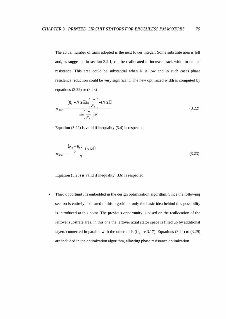
CHAPTER 3. PRINTED CIRCUIT STATORS FOR BRUSHLESS PM MOTORS 75
The actual number of turns adopted is the next lower integer. Some substrate area is left
and, as suggested in section 3.2.1, can be reallocated to increase track width to reduce
resistance. This area could be substantial when N is low and in such cases phase
resistance reduction could be very significant. The new optimized width is computed by
equations (3.22) or (3.23)
( ) ( )
NN
cNN
cNR
w
s
so
new
⋅
⋅−
⋅−
=π
π
sin
sin
(3.22)
Equation (3.22) is valid if inequality (3.4) is respected
( ) ( )N
cNRR
w
io
new
⋅−−
= 2 (3.23)
Equation (3.23) is valid if inequality (3.6) is respected
• Third opportunity is embedded in the design optimization algorithm. Since the following
section is entirely dedicated to this algorithm, only the basic idea behind this possibility
is introduced at this point. The previous opportunity is based on the reallocation of the
leftover substrate area, in this one the leftover axial stator space is filled up by additional
layers connected in parallel with the other coils (figure 3.17). Equations (3.24) to (3.29)
are included in the optimization algorithm, allowing phase resistance optimization.

CHAPTER 3. PRINTED CIRCUIT STATORS FOR BRUSHLESS PM MOTORS 76
( )/series total elementk round EMF EMF= (3.24)
where kseries = series connection coefficient (of 2-layer elements)
EMFtotal = total desired phase EMF
EMFelement = total EMF of 2-layer element
round (X) = rounds X to the nearest integer
maxa
layer
tn floor
t
=
(3.25)
where nmax = maximal number of layer
ta = stator total axial length
tlayer = layer thickness = Base cu thickness + Pre-Preg thickness
floor (X) = rounds X to the lower nearest integer
max
2parallelseries
nn floor
k
=
(3.26)
where nparallel = number of parallel layers
2u parallel seriesn n k= (3.27)
where nused = number of used layers without optimization
spiralspiral cu
spiral
lR
Aρ= (3.28)
where lspiral = length of the spiral
Aspiral = cross sectional area of the spiral

CHAPTER 3. PRINTED CIRCUIT STATORS FOR BRUSHLESS PM MOTORS 77
( ) ( ) ( )( )max max21
spiral spiralphase used serie used
parallel parallel
R RR n n k n n P
n n
= − + − − +
(3.29)
where P = number of stator poles
nmax = maximal number of layer
a)
b)
Figure 3.17 : a) Layers Structure; b) Resistive Structure
Note that difference on axial magnetic flux density between two layers is less than 0.4%.
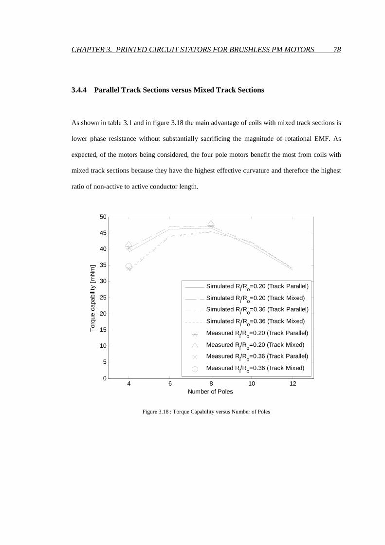
CHAPTER 3. PRINTED CIRCUIT STATORS FOR BRUSHLESS PM MOTORS 78
3.4.4 Parallel Track Sections versus Mixed Track Sections
As shown in table 3.1 and in figure 3.18 the main advantage of coils with mixed track sections is
lower phase resistance without substantially sacrificing the magnitude of rotational EMF. As
expected, of the motors being considered, the four pole motors benefit the most from coils with
mixed track sections because they have the highest effective curvature and therefore the highest
ratio of non-active to active conductor length.
Figure 3.18 : Torque Capability versus Number of Poles
4 6 8 10 120
5
10
15
20
25
30
35
40
45
50
Number of Poles
Tor
que
capa
bilit
y [m
Nm
]
Simulated Ri/Ro=0.20 (Track Parallel)
Simulated Ri/Ro=0.20 (Track Mixed)
Simulated Ri/Ro=0.36 (Track Parallel)
Simulated Ri/Ro=0.36 (Track Mixed)
Measured Ri/Ro=0.20 (Track Parallel)
Measured Ri/Ro=0.20 (Track Mixed)
Measured Ri/Ro=0.36 (Track Parallel)
Measured Ri/Ro=0.36 (Track Mixed)

CHAPTER 3. PRINTED CIRCUIT STATORS FOR BRUSHLESS PM MOTORS 79
Table 3.1 also shows that the coils with fully parallel track sections have the higher EMF
compared to coils with mixed sections. Parallel track sections have lower skew factors compared
to radial track sections which have a skew factor of 1. But the coils with parallel sections have
better pitch factors which more than compensate for the effect of their lower skew factors.
3.4.5 Single Layer Machines
In chapter 1, section 1.3, the possibility to have coils on a printed layer shared between phases
has been pointed out. Experiments have been carried out on stators with this configuration. For
fair comparison the same rotor was used as with other configurations. Since at least 6 coils must
be fitted into the layer to build a three phase machine, it is evident, that the coil pitch differs
from the magnet pitch. This results in a non sinusoidal EMF waveform (figure 3.19) and in a non
sinusoidal inductance variation (figure 3.20). Sinusoidal variation of inductance is an important
requirement of the equal inductance method which is planned to be used. From a point of view
of EMF this configuration does not achieve the same performance level as stators with mixed
track sections.

CHAPTER 3. PRINTED CIRCUIT STATORS FOR BRUSHLESS PM MOTORS 80
Figure 3.19 : Single Layer Machine Phase EMF Waveform at 1000 r/min
Figure 3.20 : Self-inductance Lbb Single Layer Stator
Based on these result the single layer machine configuration has not been considered any further.
-0.05 -0.04 -0.03 -0.02 -0.01 0 0.01 0.02 0.03 0.04 0.05-0.5
-0.4
-0.3
-0.2
-0.1
0
0.1
0.2
0.3
0.4
0.5
Time [s]
Vol
tage
[V
]
0 (1/2)*pi pi (3/2)*pi 2*pi
2.25
2.3
2.35
2.4
2.45
2.5
Rotor Position θ [el. rad]
Sel
f In
duct
ance
s [ µ
H]
Measured Lbb
Derived Sin Lbb

CHAPTER 3. PRINTED CIRCUIT STATORS FOR BRUSHLESS PM MOTORS 81
3.4.6 Number of Poles
Predictions and test results shown in table 3.1 and in figure 3.18 suggest that benefits of higher
EMF and lower phase resistance are possible if the number of poles is carefully chosen. There
are two major factors affecting the magnitude of the phase EMF. These are the magnitude of the
air-gap flux density and the total number of turns. Since the circumferential gap between
magnets, measured in electrical degrees, was kept the same irrespective of the number of poles,
there is increased leakage between neighbouring magnets as the number of poles goes up. The
consequence, as can be seen in table 3.1, is a decrease in the axial component of air-gap flux
density with higher pole numbers. The number of turns and the skew factor both go up with
number of poles. From the point of view of phase EMF, the combination of those factors results
in the existence of an optimal value for the number of poles. This optimum value is dependent
on variables such as Ri and Ro. As shown if figure 3.18, in the case of the motors being
considered, the optimum number of poles is eight.
3.4.7 Ratio of Inner Radius to Outer Radius
In the case of wound axial flux machines a well-known theoretical result stipulates that making
Ri/Ro less than 3
1 is counter productive. However this result is based on the assumption that
active sections of conductors are radial and there is a limit on the number of conductors per
meter in the circumferential direction. In the present case the active conductor sections, at least

CHAPTER 3. PRINTED CIRCUIT STATORS FOR BRUSHLESS PM MOTORS 82
near the inner radius, are not radial and therefore the 3
1 rule does not apply. Both table 3.1 and
figure 3.18 show that EMF magnitudes go up as Ri/Ro goes down, but at a decreasing rate. It has
been found that, for the chosen value of Ro, the magnitude of the phase EMF is practically
constant for values of Ri/Ro which are below about 0.2. A general conclusion would be that there
is no benefit in reducing Ri below a certain value. However that value is lower than the shaft
radius and would therefore have no practical relevance.
3.5 Design Optimization
The experimentally validated EMF evaluation method and the suggested track plotting
procedure can form the basis for a design optimization algorithm for printed circuit motors. In
the example that follows, the design objective would be to maximize torque output capability
subject to a number of constraints which are listed in Table 3.2.
The torque developed by the printed circuit motor is proportional to the product of the airgap
flux density and the stator current. At one extreme, if the entire available axial length was
allocated to the field system, torque will be zero because there would be no room left for the
stator and stator current will be zero. The other extreme would be if the entire available axial
length was allocated to the stator, excitation would be zero and again torque production would
be zero because the field flux density would be zero. As the axial length allocated to the magnet
and rotor iron is increased from zero, the output torque will rise to a maximum and then fall and

CHAPTER 3. PRINTED CIRCUIT STATORS FOR BRUSHLESS PM MOTORS 83
reaches zero again when no room is left for the stator. The aim of the algorithm is to find this
maximum.
For a given maximum stator power loss Pl, a lower phase resistance, achievable with a higher
value of ts, signifies a higher allowable stator current. Magnet axial thickness tm and phase
resistance R may be considered to be independent variables under the control of the designer.
Design optimization means identifying the (tm,R) pair that results in highest torque capability.
A design requirement is for the back EMF per unit speed to be within tight limits. Thus the
number of turns per phase, is relatively constant. In a multilayer PCB design the total number of
turns per phase, assuming all spirals are series connected, is N x L x P where N is the number of
turns in a spiral, L is the number of layers and P is the number of poles. For a given copper foil,
different (N,L) pairs satisfy the EMF requirement. For every given value of tm, a sub-optimum
is found which would correspond to the (N,L) pair that results in the highest output torque. In
cases where there is more than enough axial space to meet the EMF requirement, the algorithm
automatically increases the number of layers. The coils on the additional layers are connected in
parallel with the other coils. By paralleling the additional coils as uniformly as possible to the
other coils overall phase resistance is minimized (as introduced in section 3.4.3).

CHAPTER 3. PRINTED CIRCUIT STATORS FOR BRUSHLESS PM MOTORS 84
The algorithm consists of the following steps:
(a) Set tm equal to its minimum allowable value.
(b) Make an initial estimate for ti by simultaneous solution of equations (3.11) and (3.14).
(c) Use finite element analysis to obtain the flux density distribution and, if necessary,
repeat the FEM analysis with ti re-adjusted until the peak flux density in the rotor iron is
close to Bs.
(d) Use equation (3.14) to calculate ts.
(e) For the copper foil being considered, calculate the maximum value of N using equation
(3.3) or (3.5).
(f) For each integer value of N between 1 and its maximum value, calculate if the
constraints in Table 3.2 allow, R
PE l
m
ω.
(g) Select and plot against the current tm the highest value of R
PE l
m
ω from the current set
of values obtained from step (f).
(h) Increment tm and go to step (b) if the maximum allowable value of tm is not exceeded.
(i) Repeat steps (a) to (h) for all candidate copper foil thicknesses
(j) Read the graph from step (g) to obtain the maximum torque capability.
The graphical output from step (g) is shown in figure 3.21.
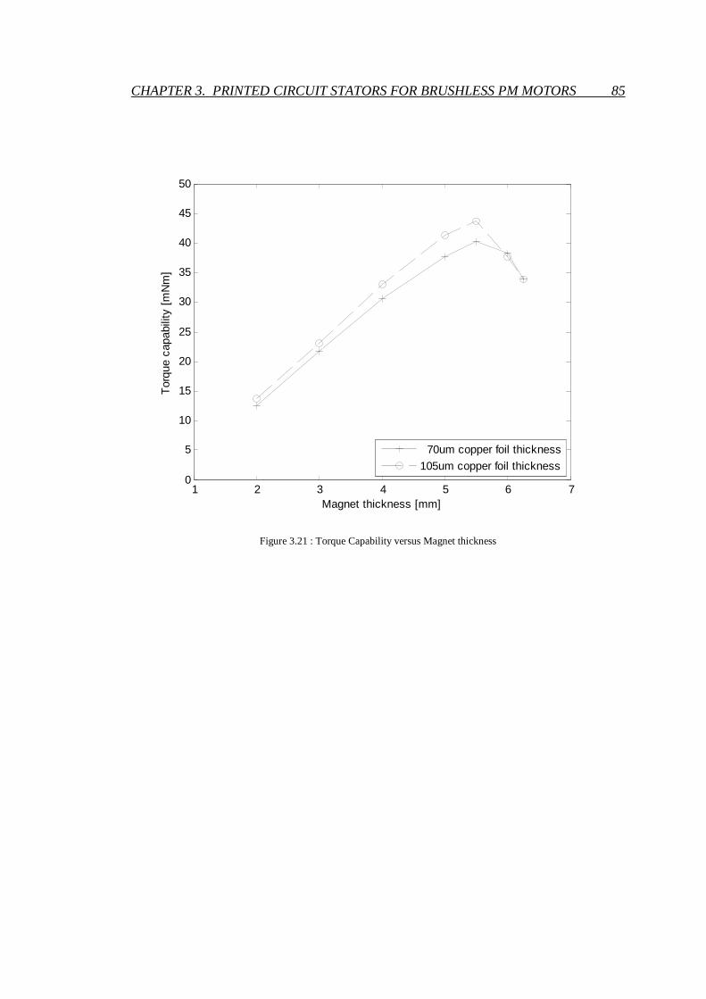
CHAPTER 3. PRINTED CIRCUIT STATORS FOR BRUSHLESS PM MOTORS 85
Figure 3.21 : Torque Capability versus Magnet thickness
1 2 3 4 5 6 70
5
10
15
20
25
30
35
40
45
50
Magnet thickness [mm]
Tor
que
capa
bilit
y [m
Nm
]
70um copper foil thickness
105um copper foil thickness

CHAPTER 3. PRINTED CIRCUIT STATORS FOR BRUSHLESS PM MOTORS 86
Table 3.2 : Printed Circuit Motor Design Example
Design Parameter Degree of Flexibility
Outer Radius (Ro) Ro = 25 mm (Ro defined in section 1)
Inner Radius (Ri) Ri = 5 mm
Number of poles (P)
P = 4
(Chosen on basis of mechanical requirement and drive switching
frequency)
Total thickness (ta) ta = 28 mm
Rotor Iron thickness (ti) ti > 1 mm (for mechanical stability)
Rotor peak flux density (Bs) Bs =1.4 T ± 0.1
Stator/Magnet Clearance (tc) 0.3 mm
Insulation layer thickness Foil 1: 100 um ; Foil 2: 100 um
Track thickness Foil 1: 70 um ; Foil 2: 105 um
Clearance between tracks Foil 1: 230 um ; Foil 2: 300 um
Minimum track width Foil 1: 200 um ; Foil 2: 300 um
Maximum track width Foil 1: 2.5 mm ; Foil 2: 2.5 mm
(to avoid stator eddy currents)
Max allowable stator power loss (Pl) Pl = 2.3 W
Magnet thickness 1mm < tm< tmax; ( tmax determined by minimum ts)
Minimum Magnet thickness delta 0.25 mm
Remanence (Br) Br = 1.24 T
EMF (at 1000 rpm) 1V ± 10%

CHAPTER 3. PRINTED CIRCUIT STATORS FOR BRUSHLESS PM MOTORS 87
3.6 Conclusions
A track plotting procedure has been developed for the design of coils in printed circuit brushless
motors. The procedure maximizes the number of turns in the printed spiral shaped coil for given
values of substrate inner radius, substrate outer radius, minimum track thickness and inter-track
clearance. Active sections of the tracks may be purely radial, parallel with each other or may be
partly radial and partly parallel. Computer programs, that implement the procedure,
automatically produce track plots which can be used directly by the printed circuit production
process.
By combining the track plotting procedure with the finite element method, a technique has been
developed to predict rotational EMF waveforms of printed circuit motors. The technique, which
has been validated by experimental results from six different prototype motors, has been used for
printed circuit motor design optimization.
.

88
Chapter 4
Sensorless Commutation Technique for
Brushless DC Motors
4
4.1 Introduction
The aim of this chapter has been to investigate the possibility of a sensorless technique which is
as cost effective as the back EMF method but with a performance at start-up comparable with
that obtained when Hall sensors are used. Initial investigations led to a saliency based method.
Unlike other proposed methods, no special signal injection is needed. The technique is based on
the detection of rotor positions where the two energised phases have equal inductances. It has
therefore been termed the equal inductance method [2]. Theoretical analysis is presented which
shows that the method is insensitive to variations in operational parameters such as load current

CHAPTER 4. SENSORLESS COM. TECHNIQUE FOR BLDC MOTORS 89
and speed or circuit parameters such as power device voltage drops and winding. Test results are
presented which demonstrate practical application of the method.
Gambetta [3] required a neutral connection for practical implementation of a version of the equal
inductance method. It is shown in this chapter that connection to the neutral is not necessary.
An initial position detection and start-up method based on saliency related measurement is also
proposed and practically implemented. This method offers starting performance as good as Hall
sensor based techniques.
4.2 Relationship between Equal Inductance Positions and
Commutation Positions
Electrical machines that exhibit saliency may be analysed using the well established two-axis
theory. This theory leads to the following expressions for the three-phase winding inductances
and mutual inductances:
( )0 2 cos 2aa aa al gL L L L θ= + + (4.1)
0 2
2cos 2
3bb aa al gL L L Lπθ = + + +
(4.2)
0 2
2cos 2
3cc aa al gL L L Lπθ = + + −
(4.3)

CHAPTER 4. SENSORLESS COM. TECHNIQUE FOR BLDC MOTORS 90
0 2
20.5 cos 2
3ab ba aa gL L L Lπθ = = − + −
(4.4)
( )0 20.5 cos 2bc cb aa gL L L L θ= = − + (4.5)
0 2
20.5 cos 2
3ac ca aa gL L L Lπθ = = − + +
(4.6)
where θ is the electrical angle between the magnetic axis of phase A and the rotor direct axis or
the rotor quadrature axis; iiL is the self inductance of phase i ; jiL is the mutual inductance
between phase i and phase j ; 0aaL , 1aL and 2gL are positive constants which are independent
of θ and, if the effects of saturation are ignored, they are also independent of winding currents.
By definition the direct axis (d-axis) of the rotor is coincident with the magnetic axis of the rotor
permanent magnet. The quadrature axis (q-axis) is ninety electrical degrees away from the d-
axis.
Equations (4.1) to (4.6) are good representation of phase inductances of BLDC motors with
surface mounted magnets or surface inset magnets. This conclusion was based on inductance
measurements performed at 20 kHz or higher on a number of test machines. Figure 4.1 shows
the phase inductance profiles for one of those machines.

CHAPTER 4. SENSORLESS COM. TECHNIQUE FOR BLDC MOTORS 91
Figure 4.1 : Measured Self-Inductances
It is important to point out that the self-inductances and the mutual inductances that are referred
to here are only effective values rather than actual values. The actual value ofaaL , for example,
can only be obtained by measurement if all circuits that are magnetically linked to phase A were
open-circuited. But that is not possible. Whilst the other two stator windings were open-
circuited, the influence of eddy-currents in the magnets and other parts of the machine could not
be eliminated. Thus the measured winding inductances are lower than their true values. They
may be regarded as effective values that take into consideration the effect of eddy-currents, in a
similar manner that the use of sub-transient inductances in synchronous machine analysis is a
0 pi/2 pi 3/2*pi 2*pi
185
190
195
200
205
210
Rotor Position θ [el. rad]
Sel
f In
duct
ance
s [ µ
H]
Laa
Lbb
Lcc

CHAPTER 4. SENSORLESS COM. TECHNIQUE FOR BLDC MOTORS 92
way of accounting for the effect of damper windings and other induced current paths on the
rotor. In the case of the test motors, induced eddy currents in the magnets result in a lower phase
inductance when the magnetic axis of that phase lines up with the magnetic axis of a rotor
magnet (direct axis). Conversely, phase inductance is a maximum when the magnetic axis of the
phase winding lines up with a quadrature axis. The reluctance is effectively less along the q-axis
because the flux cancelling effect of eddy-currents is less along that axis since the gap between
adjacent magnets breaks the eddy-currents paths. Thus the zero degree position in figure 4.1 or
in table 4.1 corresponds to alignment of the phase A magnetic axis with the rotor quadrature
axis.
Table 4.1 : Equal Inductance Positions and Commutation Intervals
Rotor position range (electrical degrees)
0
to
60
60
to
120
120
to
180
180
to
240
240
to
300
300
to
360
Energised pair in each commutation interval
CA CB AB AC BC BA
Equal inductance position before next commutation event 30 90 150 210 270 330
Next commutation position 1θ =
°60
2θ =
°120
3θ =
°180
4θ =
°240
5θ =
°300
6θ =
°360
The BLDC motor is normally operated with only two phases energised at any one time. Each
phase is energised for a 120 electrical degree interval after which it is de-energised for a 60
electrical degree interval. The ideal commutation positions,1θ to
6θ , are shown in table 4.1.
These commutation positions lead to the highest electromagnetic torque per unit ampere as well

CHAPTER 4. SENSORLESS COM. TECHNIQUE FOR BLDC MOTORS 93
as the lowest torque ripple. The reason for this is that each phase is energized during the 120
degree intervals centred about the peak value of the phase back EMF. There are six distinct
commutation intervals. They have been labelled in figure 4.1 according to the phase pair that is
energised and supply voltage polarity. For example CA corresponds to inverter transistors TB+
and TB-, shown in figure 4.2, being kept off and the other four transistors switched so that, on
average over a PWM cycle, phase terminal c is kept at a higher potential relative to phase
terminal a.
Figure 4.2 : Inverter Bridge Supplying a Brushless DC Motor
It follows from the previous paragraph that the zero-crossings of the back EMF of a particular
phase occurs 30 electrical degrees before that phase is energized. But the zero crossing of the

CHAPTER 4. SENSORLESS COM. TECHNIQUE FOR BLDC MOTORS 94
back EMF of a phase winding also coincides with alignment of the magnetic axis of that winding
with the d-axis of the rotor. Clearly at that position the self-inductance of that phase is a
minimum, whereas the inductances of the two other phases will, because of geometric
symmetry, be equal to each other. In other words, wherever the rotor d-axis aligns with the
magnetic axis of the A-phase winding, back EMF aE is equal to zero and bb ccL L= . Similar
statements can be made about the B-phase winding and the C-phase winding. Thus the positions
of equal inductance of the energized phases, just like the zero-crossings of the back EMF of the
non-energised phase occur 30 electrical degrees before the next commutation position.
There are twelve positions of equal inductance over each electrical cycle (360 electrical
degrees). Six of them correspond to the rotor q-axis coinciding with the magnetic axis of each
one of the phase windings. The other six correspond to the rotor d-axis coinciding with the
magnetic axis of each one of the phase windings. Only six of these, the ones associated with the
rotor d-axis aligning with stator phase windings will be used to help determine commutation
positions. They are specified in table 4.1. Note that while the frequency of commutation is
proportional to speed, rotor position at which commutation is initiated does not change as speed
changes.
4.3 Detection of Equal Inductance Positions
As mentioned before there are six commutation intervals. During each interval the aim is to have
only two phases active. In table 4.1 the six intervals have been labelled according to the phases

CHAPTER 4. SENSORLESS COM. TECHNIQUE FOR BLDC MOTORS 95
that are active. Transition from one interval to the next involves de-energising of one phase and
energising of the next one. This transition is complete only after the current in the outgoing
phase has decayed to zero. Decay of the current occurs through a diode and takes finite time. For
example the transition from interval AC to interval BC involves decaying current through the
diode DA-. Therefore each interval involves two sub-intervals, one during which all three-phase
currents are present and one during which the non-active phase current is equal to zero. In total
there are twelve sub-intervals and twelve corresponding inverter states. The inverter states are
labelled according to the polarity of the DC supply terminal to which the motor phase terminals
are connected. For example inverter state c+a+ b- implies the “c” and “a” phase terminals are
connected, through transistors or diodes to the positive DC rail whereas the “b” terminal is
connected to the negative DC rail. Since bipolar PWM is used, during any one of the
commutation intervals, the inverter may be in one of six possible states. For example during
interval AB, the inverter may be in state a+c+b-, or a+c-b-, or a-c+b+, or a-c-b+, or a+b-, or b+a-.

CHAPTER 4. SENSORLESS COM. TECHNIQUE FOR BLDC MOTORS 96
Figure 4.3 : Equivalent Circuits for Inverter States a+b- and b+a-
(Switching device voltage drop not shown)
The aim is to use inductive saliency to determine the correct commutation instants for the motor.
The method is based on the sensing of the potential at the non-energised phase winding terminal
after the current in that phase has decayed to zero. Consider commutation interval AB.
Assuming current ic has decayed to zero, the inverter will revert alternately between the states
a+b- and b+a-. These are represented by the equivalent circuits in figure 4.3.
Voltage measurements cyv+ and cyv− are carried out while the inverter is respectively in states a+b-
and b+a-. For consistency, as shown in figure 4.4, measurements are carried out near the middle
of the applied voltage pulses. Consecutive measurements cyv+ and cyv− are compared. It is shown,
in the next paragraphs that those two values are equal to each other at precisely the position of

CHAPTER 4. SENSORLESS COM. TECHNIQUE FOR BLDC MOTORS 97
equal inductance independent of the value of phase current, supply voltage or speed. Thus, by
cyclic monitoring of voltage signals cyv , ayv and byv , commutation instants can be pre-
determined with very little computational effort.
Figure 4.4 : Voltage Sampling Instants (st+
and st−
)
Consider operation during commutation interval AB. With the inverter in state a+b- we have:
( )1 1
2 2sy dc ay byv V v v+ + += − − (4.7)
Since ia=-ib, equation (4.7) gives:
( )2 2 2 2
bb aadc bb aa a a b asy
d L LV L L di i E Ev
dt dt
+ ++ −− + = + + −
(4.8)

CHAPTER 4. SENSORLESS COM. TECHNIQUE FOR BLDC MOTORS 98
Adding csv+ to syv+ yields:
( )2 22 2 2
2 2 2 2bb aa ca cbdc bb aa ca cb a a a b c
cy
d L L L LV L L L L di i E E Ev
dt dt
+ ++ − + −− + − + − = + + −
(4.9)
Also,
( )
( )
22 2
2
aa bb abdc a a b t a
a
aa bb ab
d L L LV i E E V i R
dtdi
dt L L L
+ + ++
+ − − − + − −
= + − (4.10)
where 2 tV+ is the total switching device voltage drop.
With the inverter in state b+a- we have:
( )1 1
2 2sy dc by ayv V v v− − −= − − (4.11)
Since ia=-ib, equation (4.11) gives:
( )2 2 2 2
bb aadc bb aa a a b asy
d L LV L L di i E Ev
dt dt
− −− −− + = + + −
(4.12)
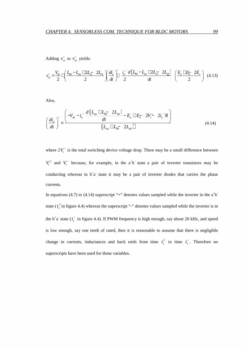
CHAPTER 4. SENSORLESS COM. TECHNIQUE FOR BLDC MOTORS 99
Adding csv− to syv− yields:
( )2 22 2 2
2 2 2 2bb aa ca cbdc bb aa ca cb a a a b c
cy
d L L L LV L L L L di i E E Ev
dt dt
− −− − + −− + − + − = + + −
(4.13)
Also,
( )
( )
22 2
2
aa bb abdc a a b t a
a
aa bb ab
d L L LV i E E V i R
dtdi
dt L L L
− − −−
+ − − − − + − −
= + − (4.14)
where 2 tV− is the total switching device voltage drop. There may be a small difference between
tV+ and tV− because, for example, in the a+b- state a pair of inverter transistors may be
conducting whereas in b+a- state it may be a pair of inverter diodes that carries the phase
currents.
In equations (4.7) to (4.14) superscript “+” denotes values sampled while the inverter in the a+b-
state ( st+ in figure 4.4) whereas the superscript “-” denotes values sampled while the inverter is in
the b+a- state (st− in figure 4.4). If PWM frequency is high enough, say about 20 kHz, and speed
is low enough, say one tenth of rated, then it is reasonable to assume that there is negligible
change in currents, inductances and back emfs from time st+ to time st
− . Therefore no
superscripts have been used for those variables.

CHAPTER 4. SENSORLESS COM. TECHNIQUE FOR BLDC MOTORS 100
If the reasonable assumption is made that (tV+ - tV− ) is negligible compared to dcV , it can be
deduced from equations (4.9), (4.10), (4.13) and (4.14) that:
2 2
2bb aa ca cb
cy cy dcaa bb ab
L L L Lv v V
L L L+ − − + −− = + −
(4.15)
Equation (4.15) confirms that, independent of all operating and machine parameters, the rotor
position at which cyv+ and cyv− are equal coincides with the position equal inductance ( aaL = bbL
and caL = cbL ).
Equation (4.15) may be written as:
( ) 53 cos 2
6
( )cos 23
dc q d
cy cy
q d q d
V L L
v v
L L L L
πθ
πθ
+ −
− + − =
+ + − +
(4.16)
where:
( )0 2
3
2q al aa gL L L L= + + (4.17)
and
( )0 2
3
2d al aa gL L L L= + − (4.18)
For reasonable saliency ratios, of around 1.2, a good approximation for (cy cyv v+ −− ) is:

CHAPTER 4. SENSORLESS COM. TECHNIQUE FOR BLDC MOTORS 101
( )
( )
53 1 cos 2
6
1
dc
cy cy
V S
v vS
πθ+ −
− + − =
+ (4.19)
S is the saliency ratio, which for the purpose of this thesis is defined as q
d
L
L. This definition has
been adopted because for the machines being considered Lq is greater than Ld.
Similarly:
( )
( )
3 1 cos 22
1
dc
ay ay
V S
v vS
πθ+ −
− − − =
+ (4.20)
and
( )
( )
3 1 cos 26
1
dc
by by
V S
v vS
πθ+ −
− + − =
+ (4.21)
Assuming a saliency ratio of 1.2 the maximum error in approximating using equation (4.19)
instead of equation (4.16) is 2.9%. It is deduced from equation (4.19) (or (4.20) or (4.21)) that
the sensitivity and precision of the equal inductance method of pre-determination of
commutation instants is dependent only on saliency ratio and the DC supply voltage. Figure 4.5
represents practical confirmation of equations (4.19) to (4.21).

CHAPTER 4. SENSORLESS COM. TECHNIQUE FOR BLDC MOTORS 102
Figure 4.5 : Measured Voltage Differences (eqs 19 - 21)
4.4 Initial Position Detection and Start-Up
Assuming the rotor is initially at standstill, the start-up procedure using the newly proposed
sensorless method consists of the following steps:
(a) Determine, by solving any two of equations (4.19) to (4.21), the two possible values for iθ ,
the rotor initial position.
(b) Identify the phase pair that on energisation will provide the maximum driving torque.
0 pi/4 pi/2 3/4*pi pi-2.5
-2
-1.5
-1
-0.5
0
0.5
1
1.5
2
2.5
Rotor Position θ [el. rad]
Vol
tage
[V
]
v+ay - v-
ay
v+by - v-
by
v+cy - v-
cy

CHAPTER 4. SENSORLESS COM. TECHNIQUE FOR BLDC MOTORS 103
(c) Energise the selected phase pair until iθ changes by a small (typically less than one
mechanical degree) but measurable amount.
(d) Depending on whetheriθ increased or decreased in step (c), determine the actual value of iθ
.
(e) Use one of equations (4.19) to (4.21) to evaluate P where:
( )( )
3 1
1dcV S
PS
−=
+ (4.22)
(f) Identify the phase pair and polarity that will provide maximum driving torque for rotation in
the desired direction.
(g) Energise the phase pair identified in step (f) and initiate commutation to the next phase pair
when the value of the measured voltage difference (left hand side of equation (4.19) or (4.20) or
(4.21)) reaches3 / 2P .
(h) Activate the normal commutation algorithm straight after initiation of the first commutation
event.
Step (a) requires at least two phase pair energisations to be done with 50 percent PWM to avoid
rotation. Any two or more of the six possible phase pair combinations could be used. A good
strategy would be to use the three pairs and polarities corresponding to equations (4.19) to (4.21)
and select two for the determination ofiθ . The third equation can be used for verification
purposes. If, for example, equations (4.19) and (4.20) were chosen to determine the rotor initial
position iθ , then we have:
1tan ( / )d s cP Pθ −= (4.23)

CHAPTER 4. SENSORLESS COM. TECHNIQUE FOR BLDC MOTORS 104
where:
1sin(2 ) 1/ 2 3 / 2cos(2 ) 1 0
cy cys i
c i ay ay
v vP P
P P v v
θθ
− + −
+ −
− − − = = −
(4.24)
In applying equations (4.19) to (4.24) together with measured voltage differences (cy cyv v+ −− ) and
( ay ayv v+ −− ), a unique value for dθ is obtained in the zero to 360 electrical degree range. The
initial rotor position iθ , however is either equal to / 2dθ or / 2dθ plus 180 electrical degrees.
The purpose of steps (b), (c) and (d), listed above, is to determine whether iθ is equal to / 2dθ
or to ( 2 ) / 2dθ π+ . The phase pair combination to be selected in step (b) should be according to
the following:
CA if 0 ≤ / 2dθ ≤ 60 ;
CB if 60 ≤ / 2dθ ≤ 120 ; and
AB if 120 ≤ / 2dθ ≤ 180 .
During step (c) the PWM duty ratio is deviated from 50% just enough to allow a small but
measurable change inθ . If θ increases then it can be deduced that / 2i dθ θ= otherwise it is
concluded that ( 2 ) / 2i dθ θ π= + .
Step (f) is about choosing the optimum phase pair for initial movement in the right direction.
This can be done according to table 4.1. For example, if the motor initial position is between
60 and 120 and backward rotation was desired, then the phase pair to be energised should be

CHAPTER 4. SENSORLESS COM. TECHNIQUE FOR BLDC MOTORS 105
BC. After the first commutation event, performed according to step (g) above, subsequent
commutation control is carried out by executing the algorithm in figure 4.6.
Figure 4.6: Commutation Algorithm Based on the Equal Inductance Method

CHAPTER 4. SENSORLESS COM. TECHNIQUE FOR BLDC MOTORS 106
4.5 Test Results
BLDC commutation based on the equal inductance method was implemented and tested using an
8 pole 12V / 2A motor (rated speed 2400 rpm). The commutation algorithm was implemented
using the 56F8013 digital signal controller.
As shown in figure 4.7(b) there is good agreement between the standstill rotor positions deduced
by solving two of equations (4.19) to (4.21) (shown in figure 4.7(a)) and the actual rotor
position. This is in spite of the existence of a small imbalance in phase inductances. The
maximum deviation between actual position and estimated position was found to be 1.4
electrical degrees.
Figure 4.7(a) : Estimated Rotor Position (360° Mechanical)
0 pi 2*pi 3*pi 4*pi 5*pi 6*pi 7*pi 8*pi-1
0
1
2
3
4
5
6
7
Rotor Position θ [el. rad]
Est
imat
ed P
ositi
on θ
[el
. ra
d]
Estimated Position

CHAPTER 4. SENSORLESS COM. TECHNIQUE FOR BLDC MOTORS 107
Figure 4.7(b) : Position Error (360° Mechanical)
Figure 4.8 shows oscillograms of phase A voltage (ayv ), phase A current, the equal inductance
flag and the commutation flag. The control software operates such that the equal inductance flag
changes state whenever the rotor passes through a position where the energised phases have
equal inductances. Thus, as expected, the equal inductance flag changes state every 60 electrical
degrees. By design the commutation flag lags the equal inductance flag by 30 electrical degrees.
The waveforms in figure 4.8 confirm correct commutations since commutation events occur
every sixty electrical degrees and disturbance of the non-commutating phase current is small.
Figure 4.9 confirms that the equal inductance method works well at higher current and higher
speed. Please note that the presented waveforms sequence (in figure 4.8 and 4.9) is identical to
the legend entries sequence.
0 pi 2*pi 3*pi 4*pi 5*pi 6*pi 7*pi 8*pi-0.02
-0.015
-0.01
-0.005
0
0.005
0.01
0.015
0.02
Actual Position θ [el. rad]
Pos
ition
Err
or [
el.
rad]
Position Error

CHAPTER 4. SENSORLESS COM. TECHNIQUE FOR BLDC MOTORS 108
Figure 4.8 : BLDC Commutation using the Equal Inductance Method (139 r/min)
Figure 4.9 : BLDC Commutation using the Equal Inductance Method (630 r/min)
-80 -40 0 40 80 120 160 200 240 280 320Time [ms]
Phase A Voltage (vay, 6V/div)
Equal Inductance Flag
Commutation Flag
Phase A Current (ia, 1A/div)
-20 -10 0 10 20 30 40 50 60 70 80Time [ms]
Phase A Voltage (vay
, 6V/div)
Equal Inductance Flag
Commutation Flag
Phase A Current (ia, 1A/div)
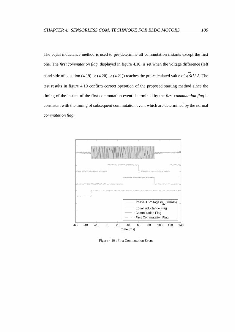
CHAPTER 4. SENSORLESS COM. TECHNIQUE FOR BLDC MOTORS 109
The equal inductance method is used to pre-determine all commutation instants except the first
one. The first commutation flag, displayed in figure 4.10, is set when the voltage difference (left
hand side of equation (4.19) or (4.20) or (4.21)) reaches the pre-calculated value of3 / 2P . The
test results in figure 4.10 confirm correct operation of the proposed starting method since the
timing of the instant of the first commutation event determined by the first commutation flag is
consistent with the timing of subsequent commutation event which are determined by the normal
commutation flag.
Figure 4.10 : First Commutation Event
-60 -40 -20 0 20 40 60 80 100 120 140Time [ms]
Phase A Voltage (vay
, 6V/div)
Equal Inductance Flag
Commutation Flag
First Commutation Flag

CHAPTER 4. SENSORLESS COM. TECHNIQUE FOR BLDC MOTORS 110
4.6 Discussion
Performance of the equal inductance method is best near zero speed since both positive and
negative PWM voltage pulses applied to the active phase pair are relatively wide. Under those
conditions, there is sufficient time for transients to settle before measurements are made. Also
there is sufficient time to perform computations. However, as speed rises either the positive
voltage pulse or the negative pulse within a PWM cycle becomes shorter and eventually there
may not be sufficient time for transients [3] to settle and for calculations to be performed. Thus
there exists an upper limit of satisfactory performance of the equal inductance method. It is not
possible to arrive at a general conclusion regarding this limit. It depends on supply voltage,
saliency, resolution and speed of the selected digital signal processor and the effect of switching
noise. With a saliency ratio of 1.1 or more, 12V DC supply and a low cost DSP with 8-bit
resolution, it is estimated that performance as good as that obtained with the back EMF zero
crossing is achievable at about 25% of full speed. Well above that speed the back EMF method
is better, whereas well below that speed the equal inductance method gives superior
performance. Thus the equal inductance method complements the back EMF very well.
The equal inductance method is based on voltage measurements made as voltage pulses are
applied to active winding pairs during bipolar operation. There is no practical advantage in
adapting the method to unipolar operation. With unipolar operation, correct measurement at very
low speed is not possible because the voltage pulse width is too short. Thus adapting the equal
inductance method to unipolar operation will not result in a technique that complements the back

CHAPTER 4. SENSORLESS COM. TECHNIQUE FOR BLDC MOTORS 111
EMF zero crossing method. If unipolar operation is preferred for normal motor operation, it is
recommended that the motor is started under bipolar operation and the equal inductance method
up to a minimum speed. Above that speed, operation can be changed to unipolar with back EMF
zero crossings used to determine commutation instants.
The equal inductance method has been found to perform very well with motors having surface
inserted magnets. However, the method can be considered for motors with fully buried magnets.
Qualitative analysis suggests that these motors would exhibit inductive saliency due to the
cumulative effects of rotor geometry and eddy currents induced in their permanent magnets.
4.7 Conclusion
A low cost saliency based sensorless technique for BLDC motors has been proposed, physically
implemented and tested. It offers performance that is equal to that obtained by systems relying
on low resolution physical devices such as Hall sensors. Rotor position is deduced from the
response of the BLDC motor un-energised phase terminal voltage, measured with respect to the
negative DC supply rail, due to bipolar PWM voltage pulses that are normally applied to the
other two phases. Theoretical analysis shows that this potential difference is made up of a DC
component equal to the sum of half the DC supply voltage and the un-energised phase back
EMF plus an AC component (non-sinusoidal) that is modulated by the rotor movement. In other
words the peak to peak value of the AC component varies as rotor position changes. The
fundamental frequency of the AC component is equal to the PWM frequency. The envelope of

CHAPTER 4. SENSORLESS COM. TECHNIQUE FOR BLDC MOTORS 112
that AC component is represented by the waveforms of figure 4.5. It was found, from the
theoretical investigation, that a zero peak to peak value of the AC component corresponds to a
rotor position that is thirty electrical degrees away from the next ideal commutation position.
That rotor position is also the one where the energized phase windings have equal inductances.
Hence the adopted sensorless commutation control method has been termed the ‘equal
inductance method’. Further theoretical analysis showed that the peak to peak value of the AC
component depends only on the DC supply voltage and the saliency ratio. In other words the
position of equal inductance deduced from voltage measurements at the un-energised phase
terminal is insensitive to operational parameters such as load current and circuit parameters such
as winding resistance.
It has been demonstrated that with sufficient saliency, standstill rotor position can be determined
from the same measurements made to determine positions of equal inductance. The necessary
phase winding energisations during those measurements may lead to some back-rotation. But
this has been found to be less than a mechanical degree and is therefore considered negligible.
Once the initial rotor position has been determined, the optimum phase pair to be energised can
be selected. Voltage measurements allow the rotor position for the first commutation event to be
identified, subsequent commutation instants being pre-determined by the ‘equal inductance
method’.
The back EMF method of commutation control relies on detection of zero-crossing instants of
the back EMF signal from the unenergised phase. It has been shown that the instant at which the
rotor reaches the equal inductance position coincides with the zero-crossing instant of the back

CHAPTER 4. SENSORLESS COM. TECHNIQUE FOR BLDC MOTORS 113
EMF of the unenergised phase. There is, therefore, a close parallel between the equal inductance
method and the back EMF method. For operation over a wide speed range it may be
advantageous to operate using the equal inductance method at low speed and the back EMF
method at high speed. The close parallel between the two methods makes it easy to implement
changeover strategies from one to the other as the motor speed crosses the chosen boundary
between low speed and high speed operation.
As pointed out in section 2.1.2 other researchers have used saliency as a basis for rotor position
detection. However, the literature review carried out the author revealed that all techniques
proposed before this thesis project were based on explicit injection of signals for the purpose of
using saliency to determine rotor position. In contrast the new method proposed in this
dissertation relies on information extracted from the normal currents and voltages of the motor.
In summary the ‘equal inductance method’ is easy to implement, is very cost competitive and
offers commutation and starting performance equal to that obtained with Hall sensors. Also, its
close parallel with the back EMF method allows seamless changeover to that method at high
speeds.

114
Chapter 5
Sensorless Commutation of Printed
Circuit Brushless DC Motors
5
5.1 Introduction
The technique proposed in chapter 4 termed the ‘equal inductance method’ offers commutation
control and starting performance equal to that obtained when using Hall sensors. However, the
method applies to nominally symmetrical machines with high enough phase winding time
constants. This chapter is about sensorless commutation of a class of motors which is
characterized by significant asymmetry and relatively low phase winding time constants. The
motors in question are axial flux machines with iron-less stators that may be wound or made up
of printed circuits. The basic reason for the asymmetry is that the three stator phases are stacked

CHAPTER 5. SENSORLESS COM. OF PRINTED CIRCUIT BLDC MOTORS 115
with each one of them located at a different axial distance from the rotor. The low phase time
constant is due to the iron-less nature of the stator. The focus in this chapter is on the printed
circuit version of the motor. A new sensorless commutation technique has been developed,
which is effectively a generalization of the originally proposed equal inductance method. The
theoretical basis behind the technique and practical results demonstrating its effectiveness are
presented.
5.2 Characteristics of Test Motors
As illustrated in chapter 3, figure 3.6, the test machines used for this thesis project had each
phase winding on separate substrates. On each substrate there is a multilayer printed circuit
which is essentially a set of spirally wound coils forming one phase of the stator.
The three substrates are nominally identical. However the magnetic axes of each substrate are
displaced from those of the other substrates by 120 electrical degrees. Details of typical printed
circuit stators were provided in chapter 3.
Two different test motors with identical rotors were used. They were both of four-pole
construction. Each substrate of both motors was made up of 8 winding layers. For test motor 1,
the spirally wound coils were arranged so that they formed two series connected groups, each
group made up of the parallel connection of half the total number of coils. For test motor 2, the
coils were arranged so that they formed two parallel connected groups, each group made up of
the series connection of half of the total number of coils. Thus, although the two test motors had

CHAPTER 5. SENSORLESS COM. OF PRINTED CIRCUIT BLDC MOTORS 116
practically the same winding time constant, the inductance and resistance of test motor 2 were
higher by a factor of approximately 4. Phase resistances of motors 1 and two were, respectively,
0.089 ohm and 0.362 ohm.
Motor inductance characteristics are of primary importance to the sensorless method being
considered. Figures 5.1 and 5.2 respectively show measured self and mutual inductances of
motor 2. As expected the self-inductance of the sandwiched or middle phase, which is phase b is
different from the self inductance of the other two phases. The two outer phases, that is phase a
and phase c, have the practically equal self–inductances. The inductances of test motor 1 behave
similarly, except as expected they are significantly smaller. As will be explained later motor 2
turned out to be a better choice because of its higher inductance. Hence it was used for most of
the subsequent tests that were carried out.
Figure 5.1 : Self-inductances of Test Motor 2
0 pi/2 pi 3/2*pi 2*pi21
22
23
24
25
26
27
28
29
30
31
32
Rotor Position θ [el. rad]
Sel
f In
duct
ance
s [ µ
H]
Derived Laa
Cos Function, Measured Laa
(*)
Derived Lbb Cos Function, Measured Lbb (+)
Derived Lcc Cos Function, Measured Lcc (o)

CHAPTER 5. SENSORLESS COM. OF PRINTED CIRCUIT BLDC MOTORS 117
Figure 5.2 : Mutual-inductances of Test Motor 2
Each set of three phase measurements of self and mutual inductances were taken for a fixed rotor
position relative to the magnetic axis of phase a. A small sinusoidal current (50mA @ 20kHz)
was injected into one phase while the other two phases were left open-circuited. The injected
current and the three line to star-point voltages were recorded. From the measurements, effective
self-inductances and mutual inductances were evaluated. As stated in chapter 3, it should be
pointed out that the self-inductances and the mutual inductances are only effective values rather
than actual values because they incorporate the effect of eddy-currents in permanent magnets
and the rotor iron.
Electrical machines that exhibit saliency and that are symmetrical may be analyzed using the
well established two-axis theory. Equations (5.1) to (5.6) below are modified versions of the
0 pi/2 pi 3/2*pi 2*pi-18
-16
-14
-12
-10
-8
-6
Rotor Position θ [el. rad]
Mut
ual I
nduc
tanc
es [ µ
H]
Derived Lab
Cos Function, Measured Lab
(*)
Derived Lbc
Cos Function, Measured Lbc
(+)
Derived Lac
Cos Function, Measured Lac
(o)

CHAPTER 5. SENSORLESS COM. OF PRINTED CIRCUIT BLDC MOTORS 118
classical equations that are based on the two-axis theory. The modifications allow for the
asymmetry that is characteristic of the class of machines under consideration. The terms ∆Ls2,
∆Ls0, ∆Lm0 and ∆Lm2 that appear in the equations represent the necessary modifications. For test
motor 2, in µH, Ls0=27.82; Ls2=3.08; ∆Ls0=0.27; ∆Ls2=6.46; Lm0=1.14; Lm2=2.76; ∆Lm0=3.15
and ∆Lm2=0.36.
( )0 2 cos 2aa s sL L L θ= + (5.1)
( ) ( )0 0 2 2
2cos 2
3bb s s s sL L L L Lπθ = + ∆ + − ∆ +
(5.2)
0 2
2cos 2
3cc s sL L Lπθ = + −
(5.3)
0 2
2cos 2
3ab ba m mL L L Lπθ = = − + −
(5.4)
( )0 2 cos 2bc cb m mL L L L θ= = − + (5.5)
( ) ( )0 0 2 2
2cos 2
3ca ac m m m mL L L L L Lπθ = = − − ∆ + − ∆ +
(5.6)
5.3 Determination of commutation positions
Figure 5.3 represents the printed windings of a BLDC motor connected to a three-phase bridge.
The commutation intervals are defined in table 5.1. The rotor is considered to be at zero angular
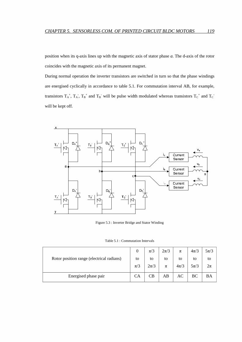
CHAPTER 5. SENSORLESS COM. OF PRINTED CIRCUIT BLDC MOTORS 119
position when its q-axis lines up with the magnetic axis of stator phase a. The d-axis of the rotor
coincides with the magnetic axis of its permanent magnet.
During normal operation the inverter transistors are switched in turn so that the phase windings
are energised cyclically in accordance to table 5.1. For commutation interval AB, for example,
transistors TA+, TA
-, TB+ and TB
- will be pulse width modulated whereas transistors TC+ and TC
-
will be kept off.
Figure 5.3 : Inverter Bridge and Stator Winding
Table 5.1 : Commutation Intervals
Rotor position range (electrical radians)
0
to
π/3
π/3
to
2π/3
2π/3
to
π
π
to
4π/3
4π/3
to
5π/3
5π/3
to
2π
Energised phase pair CA CB AB AC BC BA

CHAPTER 5. SENSORLESS COM. OF PRINTED CIRCUIT BLDC MOTORS 120
As for the equal inductance method presented in chapter 4, bipolar pulse width modulation
(PWM) is assumed. The selected PWM frequency was 20 kHz. This means that a relatively large
number of PWM cycles fits into one commutation interval. During interval AB, TA+ and TB
- are
normally turned on for a longer portion of the PWM period to achieve a positive average for vab.
Conversely during interval BA, TA- and TB
+ are normally turned on for a larger portion of the
PWM period to achieve a negative average value for vab. Voltage vab is defined in figure 5.4.
Assuming conduction takes place through two legs of the inverter, there would be six states that
the inverter could be in. These are labelled a+b-, b+a-, b+c- and c+b-, c+a- and a+c-. For example
during state a+b-, transistors TA+ and TB
- are turned on. Figure 5.4 shows the motor equivalent
circuits for inverter states a+b- and b+a-.
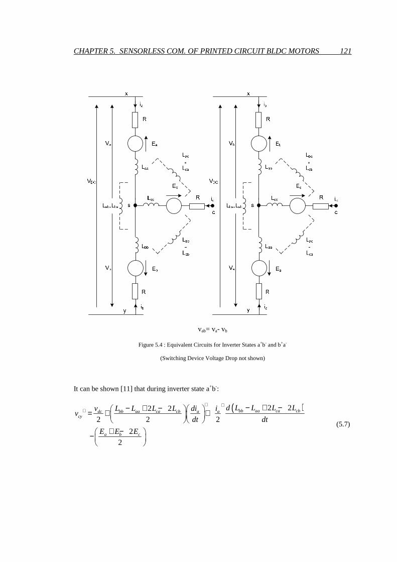
CHAPTER 5. SENSORLESS COM. OF PRINTED CIRCUIT BLDC MOTORS 121
vab= va- vb
Figure 5.4 : Equivalent Circuits for Inverter States a+b- and b+a-
(Switching Device Voltage Drop not shown)
It can be shown [11] that during inverter state a+b-:
( )2 22 2
2 2 2
2
2
bb aa ca cbdc bb aa ca cb a acy
a b c
d L L L Lv L L L L di iv
dt dt
E E E
+ ++ − + −− + − = + +
+ − −
(5.7)
CHAPTER 5. SENSORLESS COM. OF PRINTED CIRCUIT BLDC MOTORS 122
( )
( )
22 2
2
aa bb abdc a a b t a
a
aa bb ab
d L L Lv i E E v i R
dtdi
dt L L L
+ + ++
+ − − − + − −
= + − (5.8)
Similarly during inverter state b+a-:
( )2 22 2
2 2 2
2
2
bb aa ca cbdc bb aa ca cb a acy
a b c
d L L L Lv L L L L di iv
dt dt
E E E
− −− − + −− + − = + +
+ − −
(5.9)
( )
( )
22 2
2
aa bb abdc a a b t a
a
aa bb ab
d L L Lv i E E v i R
dtdi
dt L L L
− − −−
+ − − − − + − −
= + − (5.10)
In equations (5.7) to (5.10), superscript ‘+’ denotes values sampled while the inverter is in state
a+b-whereas superscript ‘-’ denotes values sampled while the inverter is in state b+a-. The values
of currents and voltages referred to in equations (5.7) to (5.10) are sampled within a single PWM
cycle. Total switching device voltage drop is denoted by 2vt+ for inverter state a+b- and by 2vt
-
for inverter state b+a-. It is reasonable to assume that rotational back EMFs Ea, Eb and Ec remain
unchanged during a PWM cycle.
If, as shown in figure 5.5, voltage is sampled at the same level of winding current during inverter
state a+b- and b+a-, we can deduce, from equation (5.7) to (5.10), that:
2 2
2bb aa ca cb
cy cy dcaa bb ab
L L L Lv v v
L L L+ − − + −− = + −
(5.11)

CHAPTER 5. SENSORLESS COM. OF PRINTED CIRCUIT BLDC MOTORS 123
( ) ( ) ( )
( ) ( )
2 2 2 2
0 0 0 2 2 2
5 22 3 2 cos 2 2 cos 2
6 3
22 2 2 cos 2 cos 2
3 3
dc so mo s m s m
cy cy
s m s s m s
v L L L L L L
v v
L L L L L L
π πθ θ
π πθ θ
+ −
∆ + ∆ + + + − ∆ + ∆ + − =
+ + ∆ + + + − ∆ +
(5.12)
Equation (5.11) is based on the reasonable assumption that |vt+- vt
-| is much smaller than vdc.
Also inspection of equation (5.7) and (5.10) reveals that, theoretically, making ia+ equal to ia
-
results in complete insensitivity of the measured voltage difference to phase resistance.
Figure 5.5 : Voltage Sampling Instants (ts+ and ts
-)
Figure 5.5 illustrates the fundamental difference between the equal inductance method
introduced in chapter 4, and the method proposed in this chapter. Voltage vcy is first sampled at
time instant ts+ during inverter state a+b-. The current ia
+, also sampled at ts+, is termed the
threshold current. In practice, to avoid errors associated with ringing caused by parasitic

CHAPTER 5. SENSORLESS COM. OF PRINTED CIRCUIT BLDC MOTORS 124
capacitances and inductances, ts+ must be sufficiently delayed from the instant that the inverter
changes state. Voltage vcy is then sampled at ts-, at which instant current ia must be equal to the
threshold value recorded at ts+. In contrast, with the equal inductance method, ts
+ and ts- were
chosen to be in the middle of the applied voltage pulses, the implicit assumption being that the
winding current was practically equal at those two instants. This assumption is only true if the
winding time constant is long compared with the PWM period.
In practice identification of ts- is carried out by continuous sampling of vcy and the winding
current before the latter crosses the threshold current. Each current sample is compared with the
threshold current. When the sampled current goes below the threshold current, sampling is
stopped, ts- is deemed to have been identified and vcy
- is taken to be equal to the average of the
last two samples of vcy.
While equations (5.11) and (5.12) are applicable when phase c is idle, equations (5.13) and
(5.14) apply when phase a is idle and equations (5.15) and (5.16) apply when phase b is idle.
2 2
2cc bb ab ac
ay ay dcbb cc bc
L L L Lv v v
L L L+ − − + −− = + −
(5.13)
( ) ( ) ( )
( ) ( ) ( )
2 2 2 2
0 0 0 2 2 2
22 3 2 cos 2 2 cos 2
2 3
22 2 2 cos 2 cos 2
3
dc so mo s m s m
ay ay
s m s s m s
v L L L L L L
v v
L L L L L L
π πθ θ
πθ θ
+ −
−∆ − ∆ + + − + ∆ + ∆ + − =
+ + ∆ − + − ∆ +
(5.14)
2 2
2aa cc bc ba
by by dccc aa ca
L L L Lv v v
L L L+ − − + −− = + −
(5.15)

CHAPTER 5. SENSORLESS COM. OF PRINTED CIRCUIT BLDC MOTORS 125
( )
( ) ( )
2 2
0 0 0 2 2 2
3 2 cos 26
2 2 2 2 2 cos 23
dc s m
by by
s m m s m m
v L Lv v
L L L L L L
πθ
πθ
+ −
+ + − =
+ − ∆ + + − ∆ −
(5.16)
It is now shown that there are unique relationships between the phase voltage differences defined
by equations (5.12), (5.14) and (5.16) and the commutation positions given in figure 5.6.
Figure 5.6 : Relationship between Voltage Zero Crossings and Commutation Positions
Equation (5.16) will be considered first. With vby+ equal to vby
- we have:
cos 2 06
πθ + =
(5.17)
0 pi/2 pi 3/2*pi 2*pi-6
-5
-4
-3
-2
-1
0
1
2
3
Rotor Position θ [el. rad]
Vol
tage
[V
]
v+by-v-
by theoretical
v+ay-v-
ay theoretical
v+cy-v-
cy theoretical
C+A - C+B- A+B- A+C- B+C- B+A-
Commutation
α β α β δ δ

CHAPTER 5. SENSORLESS COM. OF PRINTED CIRCUIT BLDC MOTORS 126
Within the range from 0° to 360°, the solutions to equation (5.17) are 30°, 120°, 210° and 300°.
Those four solutions appear in figure 5.6. It is clear that two of the solutions, θ=120° and
θ=300°, are not applicable to the detection of the commutation instant because at these positions
vby is not being measured. On the other hand, as shown in figure 5.6, vby is being measured
during commutation intervals CA or AC. The points at which vby+ equals vby
- occur in the middle
of those intervals respectively at θ=30° and at θ=210°. This means that by monitoring the
voltage of the b-phase while the other two phases are energised, the next commutation instants
can be determined. It is clear from figure 5.6 that if the motor is going through commutation
interval CA and AC, the next commutation position is thirty electrical degrees away from the
position when (vby+ - vby
-) is equal to zero. It is interesting to note that the position at which vby+
is equal to vby- is also the position where Laa is equal to Lcc. This is due to the fact that the middle
phase, which is the b-phase, is symmetrically positioned relative to the other two phase
windings. So detection of commutation positions while outer phases a and c are energised
resembles the standard equal inductance method (chapter 4).
Determination of commutation positions at the end of commutation intervals AB and BA is
based on the solution to equation (5.12). Samples of voltage vcy are taken until vcy+ is found to be
equal to vcy-. Under that condition equation (5.12) reduces to:
( ) ( ) ( )2 2 2 2
5 22 3 2 cos 2 2 cos 2 0
6 3so mo s m s mL L L L L Lπ πθ θ ∆ + ∆ + + + − ∆ + ∆ + =
(5.18)

CHAPTER 5. SENSORLESS COM. OF PRINTED CIRCUIT BLDC MOTORS 127
The solution to equation (5.18) is given by:
( )( ) ( ) ( ) ( )
( ) ( )
( ) ( )
1
2 2
2 2 2 2 2 2 2 2
2 2 2 2
1
2 2 2 2
2sin
2 2 3 2 23
2 2
2
3 2 2
2tan
2 23
2
2
so mo
s m s m s m s m
s m s m
s m s m
L L
L L L L L L L L
L L L L
L L L L
θ δ
−
−
−∆ − ∆ − + + ∆ + ∆ − + + ∆ + ∆ + = =
− + + ∆ + ∆ − + + ∆ + ∆ −
(5.19)
Similarly determination of commutation positions at the end of commutation intervals CB or BC
is based on the solution to equation (5.14). Samples of voltage vay are taken until vay+ is found to
be equal to vay-. Under that condition equation (5.14) reduces to:
( ) ( ) ( )2 2 2 2
22 3 2 cos 2 2 cos 2 0
2 3so mo s m s mL L L L L Lπ πθ θ −∆ − ∆ + + − + ∆ + ∆ + =
(5.20)
The solution to equation (5.20) is given by:

CHAPTER 5. SENSORLESS COM. OF PRINTED CIRCUIT BLDC MOTORS 128
( )
( ) ( ) ( )
( )
( ) ( )
1
2 2
2 2 2 22 2
2 2
1
2 22 2
2sin
2 23 2
2 2
2
2
2tan2
3 22
2
so mo
s m s ms m
s m
s ms m
L L
L L L LL L
L L
L LL L
θ β
−
−
+∆ + ∆ ∆ + ∆ ∆ + ∆ + − + − = =
∆ + ∆ − ∆ + ∆ + − −
(5.21)
The angular positions at which equations (5.18) and (5.20) are satisfied are shown on figure 5.6.
Equations (5.19) and (5.21) emphasize that those positions are independent of operating
conditions. Since the positions at which equations (5.18) and (5.20) are satisfied are fixed,
measurements of vay and vcy can be used to determine commutation positions. Referring to figure
5.6, during commutation interval AB or BA, the commutation controller can be programmed to
carry out the next commutation (Π/3 - δ) or β radians from the instant when equation (5.18) is
satisfied. Similarly during interval BC or CB, the commutation controller can be programmed to
carry out the next commutation (Π/3- β) or δ radians from the instant when equation (5.20) is
satisfied.

CHAPTER 5. SENSORLESS COM. OF PRINTED CIRCUIT BLDC MOTORS 129
5.4 Initial Position Detection
Determination of initial position by the equal inductance method (presented in chapter 4) is
entirely based on on-line measurements. The controller does not have to rely on stored motor
data. However a basic assumption is that motor is symmetrical. In the case of a motor that is not
symmetrical it is impossible to determine the initial rotor position solely from measured voltages
such as those defined by equations (5.12), (5.14) and (5.16). One solution to the problem is to
pre-load five motor constants into the controller memory.
These are:
( )( )
2 21
0 0 0
3 2
2 2 2s m
s m m
L Lk
L L L
+=
+ − ∆; (5.22)
( )( )
2 22
0 0 0
3 2
2 2s m
s m s
L Lk
L L L
+=
+ + ∆ ; (5.23)
( )( )
2 23
0 0 0
2
2 2s m
s m s
L Lk
L L L
∆ + ∆=
+ + ∆ ; (5.24)
( )( )
0 04
0 0 0
2
2 2s m
s m s
L Lk
L L L
∆ + ∆=
+ + ∆ and (5.25)
5k β= which is defined in figure 5.6. (5.26)
Motor constants k1 to k4 are coefficients from the right hand side of equations (5.12), (5.14) and
(5.16). They are derived under the assumption that the cosine terms in the denominator of those
equations are negligible. Figure 5.7 compares waveforms calculated using equations (5.12),
(5.14) and (5.16) with and without the cosine terms in the denominator.

CHAPTER 5. SENSORLESS COM. OF PRINTED CIRCUIT BLDC MOTORS 130
Figure 5.7 : Voltage Difference Waveforms (full equations and simplified)
It has been found that neglecting the cosine term leads to a maximum starting position
estimation error of 4 electrical degrees. It does not however contribute to any error in the
determination of commutation positions after start-up, since at the “zero crossing” positions, the
error disappears. There is a possibility to avoid this error, by implementing bi-dimensional look-
up tables representing equations (5.12), (5.14) and (5.16) in discrete from. If the acquired
voltage samples are properly scaled, they define the indices to directly access the look-up tables.
Doing this the method will lose some flexibility but would still keep the computation burden to
an acceptable level. However the pre-operative operations to generate and link the look-up tables
will be significant. This possibility has also been tested, but not further considered, due to the
above mentioned drawbacks.
0 pi/2 pi 3/2*pi 2*pi
-6
-5
-4
-3
-2
-1
0
1
2
3
4
Rotor Position θ [el. rad]
Vol
tage
[V
]
v+by-v-
by, o (constant denominator)
v+ay-v-
ay, + (constant denominator)
v+cy-v-
cy, x (constant denominator)

CHAPTER 5. SENSORLESS COM. OF PRINTED CIRCUIT BLDC MOTORS 131
Motor constants k1, k2 and k3 are coefficients of the cosine terms in equations (5.16), (5.12) and
(5.14) respectively. Motor constant k4 is the first bracketed term of equation (5.12). The
determination of constants k1 to k5 off-line and their pre-loading into the digital controller greatly
reduces the computational burden during on-line calculations. Experimental methods to
determine the motor constants are presented in chapter 7. Sensitivity analysis can be carried out
based on differences between predicted values and measured values.
Assuming the rotor is initially at standstill, start-up would consist of the following steps:
a) Determine, by solving any two of equations (5.12), (5.14) and (5.16), the two possible
values for θi, the rotor initial position.
b) Identify the phase pair that on energisation will provide the maximum driving torque.
c) Energise the selected phase pair until θi changes by a small (typically less than one
mechanical degree) but measurable amount.
d) Depending on whether θi is increased or decreased in step (c), determine the actual value of
θi.
e) Identify the phase pair and polarity that will provide maximum driving torque for rotation in
the desired direction.
f) Energise the phase pair identified in step (e) and initiate commutation to the next phase pair
when the value of the measured voltage difference reaches the value specified in table 5.2.
g) Activate the normal commutation algorithm straight after initiation of the first commutation
event.

CHAPTER 5. SENSORLESS COM. OF PRINTED CIRCUIT BLDC MOTORS 132
Table 5.2: Value of sensed Voltage Differences at First Commutation Positions
Phase pair
first energised
as per step (e)
Voltage
difference
sensed
Voltage value at first
commutation position
(forward)
Voltage value at first
commutation position
(reverse)
CA or AC by by
dc
v v
v
+ −− 1
5sin
6k
π
1 sin
6k
π
CB or BC ay ay
dc
v v
v
+ −− 4 1 3
5cos
6k k k
π − + +
4 1 3
2cos cos
6 3k k k
π π − + −
AB or BA cy cy
dc
v v
v
+ −− 4 1 3
5 2cos cos
6 3k k k
π π + −
4 1 3cos
6k k k
π − + −
As in the case of the standard equal inductance method, step (a) requires at least two phase pair
energisations to be carried out with 50 percent PWM duty cycle to avoid rotation. Any two of
the six possible phase pair combinations could be used. A third one can be used for verification
purposes. If, for example, phase pair AB and BC were used equations (5.12) and (5.14) would
apply and we would have:
1tan sd
c
P
Pθ −
=
(5.27)
( )( )
1
42 3 2 3
2 3 3 4
5 2 5 2sin sin cos cos
sin 2 6 3 6 3
cos 2 2 2sin cos
3 3
cy cy
dcs i
c i ay ay
dc
v vkk k k k
vP
P v vk k k k
v
π π π πθθ π π
− + −
+ −
− −− + − = = − − +
(5.28)

CHAPTER 5. SENSORLESS COM. OF PRINTED CIRCUIT BLDC MOTORS 133
Equations (5.27) and (5.28) define a unique value for θd in the zero to 360 electrical degree
range. The initial rotor position θi, however is either equal to θd/2 or (θd+2π)/2. The purpose of
steps (b), (c) and (d), listed above, is to determine whether θi is equal to θd/2 or (θd+2π)/2.
The phase pair combination to be selected in step (b) should be:
CA if 0 /32dθ π≤ < ;
CB if / 3 2 / 32dθπ π≤ < ; and
AB if 2 /32dθπ π≤ < .
Step (c) requires the PWM duty ratio to be deviated from 50% just enough to allow a small but
measurable change in rotor position. It can be deduced that θi = θd/2 if θ increases, otherwise θi =
(θd+2π)/2.
Step (e) is about the choice of the first phase pair to be energised. This can be done with the help
of table 5.2. For example, if the rotor initial position is between 120° and 180° and backward
rotation was desired, then the phase pair to be energised should be BA. The first commutation
event is performed according to step (f) above and subsequent commutation is carried out as
described in section 5.3.
The procedure for the determination of the initial position has, by design, very much the same
structure as the one presented in the previous chapter.
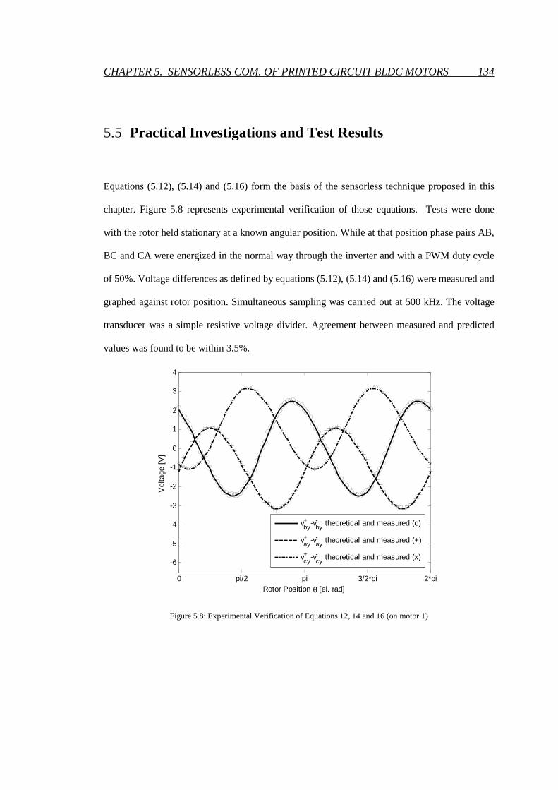
CHAPTER 5. SENSORLESS COM. OF PRINTED CIRCUIT BLDC MOTORS 134
5.5 Practical Investigations and Test Results
Equations (5.12), (5.14) and (5.16) form the basis of the sensorless technique proposed in this
chapter. Figure 5.8 represents experimental verification of those equations. Tests were done
with the rotor held stationary at a known angular position. While at that position phase pairs AB,
BC and CA were energized in the normal way through the inverter and with a PWM duty cycle
of 50%. Voltage differences as defined by equations (5.12), (5.14) and (5.16) were measured and
graphed against rotor position. Simultaneous sampling was carried out at 500 kHz. The voltage
transducer was a simple resistive voltage divider. Agreement between measured and predicted
values was found to be within 3.5%.
Figure 5.8: Experimental Verification of Equations 12, 14 and 16 (on motor 1)
0 pi/2 pi 3/2*pi 2*pi
-6
-5
-4
-3
-2
-1
0
1
2
3
4
Rotor Position θ [el. rad]
Vol
tage
[V
]
v+by
-v-by
theoretical and measured (o)
v+ay
-v-ay
theoretical and measured (+)
v+cy
-v-cy
theoretical and measured (x)
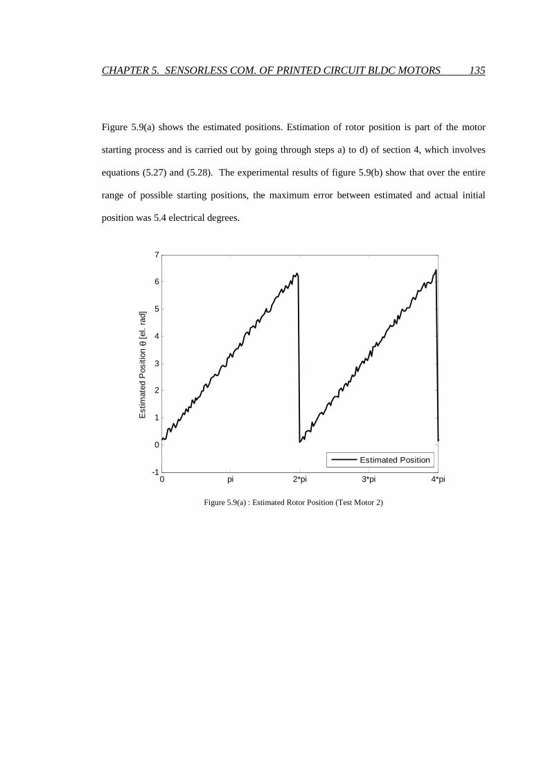
CHAPTER 5. SENSORLESS COM. OF PRINTED CIRCUIT BLDC MOTORS 135
Figure 5.9(a) shows the estimated positions. Estimation of rotor position is part of the motor
starting process and is carried out by going through steps a) to d) of section 4, which involves
equations (5.27) and (5.28). The experimental results of figure 5.9(b) show that over the entire
range of possible starting positions, the maximum error between estimated and actual initial
position was 5.4 electrical degrees.
Figure 5.9(a) : Estimated Rotor Position (Test Motor 2)
0 pi 2*pi 3*pi 4*pi-1
0
1
2
3
4
5
6
7
Est
imat
ed P
ositi
on θ
[el
. ra
d]
Estimated Position
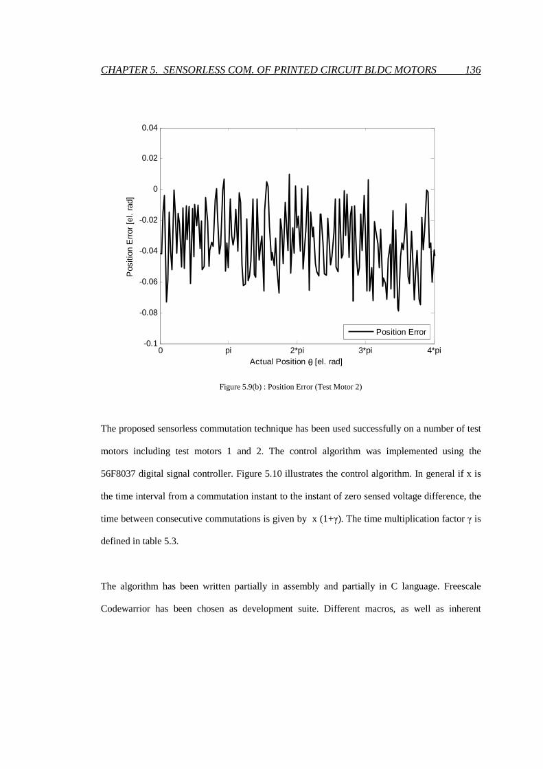
CHAPTER 5. SENSORLESS COM. OF PRINTED CIRCUIT BLDC MOTORS 136
Figure 5.9(b) : Position Error (Test Motor 2)
The proposed sensorless commutation technique has been used successfully on a number of test
motors including test motors 1 and 2. The control algorithm was implemented using the
56F8037 digital signal controller. Figure 5.10 illustrates the control algorithm. In general if x is
the time interval from a commutation instant to the instant of zero sensed voltage difference, the
time between consecutive commutations is given by x (1+γ). The time multiplication factor γ is
defined in table 5.3.
The algorithm has been written partially in assembly and partially in C language. Freescale
Codewarrior has been chosen as development suite. Different macros, as well as inherent
0 pi 2*pi 3*pi 4*pi-0.1
-0.08
-0.06
-0.04
-0.02
0
0.02
0.04
Actual Position θ [el. rad]
Pos
ition
Err
or [
el.
rad]
Position Error

CHAPTER 5. SENSORLESS COM. OF PRINTED CIRCUIT BLDC MOTORS 137
functionalities of the Freescale 56F8XXX DSC family, have been used, for example to access
the ad converter module.
Figure 5.11 shows the waveforms of the current of phase b captured while the test motors were
operating at 750 rpm. The current waveform provides evidence of correct operation of the
proposed sensorless technique with commutation events taking place every 60 electrical degrees.
Figure 5.11 also shows the relationship between actual commutation instants and the instants of
detecting of zero voltage differences. Note that tα, tβ and tδ corresponds respectively to angles α,
β and δ of figure 5.6. The higher ripple content in the current waveform of test motor 1 is a
reflection of its lower inductance.

CHAPTER 5. SENSORLESS COM. OF PRINTED CIRCUIT BLDC MOTORS 138
Figure 5.10 : Commutation Control Algorithm

CHAPTER 5. SENSORLESS COM. OF PRINTED CIRCUIT BLDC MOTORS 139
a)
b)
Figure 5.11 : Commutation under Load at 750 rpm, a) Motor 1, b) Motor 2
0 5 10 15 20 25 30 35 40 45Time [ms]
Phase Current (ib, 5A/div)
Zero Crossing A (v+ay-v-
ay, 5V/div)
Zero Crossing B (v+by-v-
by, 5V/div)
Zero Crossing C (v+cy-v-
cy, 5V/div)
0 5 10 15 20 25 30 35 40 45Time [ms]
Phase Current (ib, 5A/div)
Zero Crossing A (v+ay-v-
ay, 5V/div)
Zero Crossing B (v+by-v-
by, 5V/div)
Zero Crossing C (v+cy-v-
cy, 5V/div)
C+A- C+B- A+B-
A+C-
B+C- B+A-
tβ
tα tδ
C+A-
C+A- C+B- A+B-
A+C-
B+C- B+A-
tβ
tα tδ
C+A-

CHAPTER 5. SENSORLESS COM. OF PRINTED CIRCUIT BLDC MOTORS 140
Table 5.3 : Commutation Time Multiplier γ 3
πβ δ = −
Commutation interval CA or AC CB or BC AB or BA
γ forward rotation 1 δβ
βδ
γ reverse rotation 1 βδ
δβ
It is important to mention that the first commutation is much easier than a commutation during
the running mode because the commutation take place immediately after the pre-loaded voltage
threshold (table 5.2) is reached. This is done in hardware by a dedicated interrupt subroutine,
called automatically after crossing of the pre-loaded voltage threshold value.
While successful commutation and start-up were obtained with both test motor 1 and test motor
2, it was noted that test motor 1, because of its lower inductance and resistance presented a
higher burden on the inverter and power supply during start-up. The technique used to determine
initial position relies on the application of what is essentially a square wave to winding pairs
(essentially an R-L circuit) and this results in a non-sinusoidal AC component in the winding
current (rising and falling exponential). Figure 5.12 presents the waveform on motor 1 during
start-up. There is a need to ensure that the inverter transistors and the DC source are rated to
supply this AC current component.

CHAPTER 5. SENSORLESS COM. OF PRINTED CIRCUIT BLDC MOTORS 141
Figure 5.12 : Motor 1 Waveforms
5.6 Practical Considerations
5.6.1 Motor Stiction
BLDC sensorless control strategies are useful and justified in applications where no holding
torque at 0 speed is required for example in the case of fans and pumps. During the first two
steps of the start-up procedure, the proposed method is not sensitive to the load conditions, since
a 50% duty cycle is applied, which does not result in any rotation. However in step c), if the load
-40 -20 0 20 40Time [µs]
Applied Phase Voltage (vab, 5V/div)
Sensed Voltage (vcy, 2V/div)
Phase Current (ia, 5A/div)

CHAPTER 5. SENSORLESS COM. OF PRINTED CIRCUIT BLDC MOTORS 142
is too heavy, the rotor will not move. In order to prevent serious damage to the inverter, a fault /
warning signal (over current) will be automatically generated.
5.6.2 Power Semiconductor Voltage Drops Compensation
Equation (5.11) which is obtained from equations (5.7) to (5.10), shows that voltage drop across
power switches do not have any significant influence as long as the difference in voltage drop
across the power switches during the two states of a PWM cycle is small compared to the DC
supply voltage. However, a part of the control algorithm is dedicated to a direct compensation of
these voltage drops, regardless of their amplitude.
The coreless nature of the machine being considered means they have relatively short time
constants. Consequently the current in the outgoing phase decays to zero in the first few PWM
pulses after commutation. Generally speaking, after commutation, the first few pulses can be
discarded without influencing the drive performance, since the PWM frequency is much higher
than the phase winding commutation frequency. The choice of the PWM frequency is not only
important for that aspect but also from a point of view of the sampling resolution, since, as
introduced above, the simultaneous sampling frequency is 500 kHz. If the selected PWM
frequency is too high, the resolution could significantly decrease, affecting drive performance.
The sampling frequency of 500 kHz is limited by the bandwidth of the DSC analog to digital
converter. Simultaneous sampling is fundamental in order to have time consistent data to
process.

CHAPTER 5. SENSORLESS COM. OF PRINTED CIRCUIT BLDC MOTORS 143
The following list introduces the main sampling characteristics:
• Sampling enabled 3.75 µs (approximately 7.5% of PWM period) after commutation to
avoid “ringing”
• Three values are acquired simultaneously (for example: ia, vab and vcy)
• Per definition, in the “first pulse”, the samples are acquired “only” at time instant = 5 µs
(10% of PWM period)
• The acquired value of ia sets the “current threshold” for “second pulse” acquisition
• In the “second pulse”, samples are taken every 2 µs (max. sampling rate)
• Sampling is stopped once the sampled (actual) ia crosses the “current threshold”; values
of actual sampling instant and of (instant-1) are considered and linearly interpolated to
increase precision
• Special hardware functionalities of the DSC are used. They notably accelerate data
processing, e.g. automatic interrupt ISR call on threshold value crossing.
After having introduced the sampling characteristics, the focus is set back to the voltage drop
cancellation strategy.
Consider figure 5.13: in every pulse (tON or tOFF of the applied PWM pulse) two different
intervals can be distinguished:
a) Current fast (forced) decaying through the free-wheeling diodes. During this interval the
voltage level at motor phase terminals are pushed above / below (symmetrically) the dc-
rails references voltages because of the freewheeling diodes voltage drops. As the
current decays the voltage shift is reduced following the diode’s characteristics.
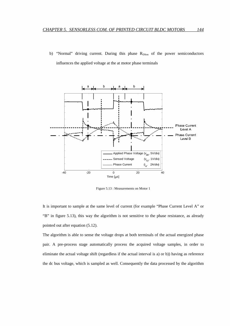
CHAPTER 5. SENSORLESS COM. OF PRINTED CIRCUIT BLDC MOTORS 144
b) “Normal” driving current. During this phase RDSon of the power semiconductors
influences the applied voltage at the at motor phase terminals
-40 -20 0 20 40Time [µs]
Applied Phase Voltage (vab, 5V/div)
Sensed Voltage (vcy, 1V/div)
Phase Current (ia, 2A/div)
Figure 5.13 : Measurements on Motor 1
It is important to sample at the same level of current (for example “Phase Current Level A” or
“B” in figure 5.13), this way the algorithm is not sensitive to the phase resistance, as already
pointed out after equation (5.12).
The algorithm is able to sense the voltage drops at both terminals of the actual energized phase
pair. A pre-process stage automatically process the acquired voltage samples, in order to
eliminate the actual voltage shift (regardless if the actual interval is a) or b)) having as reference
the dc bus voltage, which is sampled as well. Consequently the data processed by the algorithm

CHAPTER 5. SENSORLESS COM. OF PRINTED CIRCUIT BLDC MOTORS 145
are consistent with the value computed with the dc-bus voltage as a reference. Due to this easy
pre-processing step there is no need to modify any of the presented equations, giving full system
stability also if a low cost semiconductor presenting a large value of RDSon is used.
If the voltage shifts (on the motor terminals) are be considered as dc-bus voltage ripple, the pre-
process stage can be considered as a dc-bus ripple cancellation stage.
5.6.3 Computation Burden and Speed Range
During rotation, multiplication factor γ is used (Table 5.3 and Figure 5.11). This way the DSC is
not loaded with “heavy” computations, since the multiplication factors are determined off-line
based on equations (5.19) and (5.21). An online computation would not be possible with the
proposed DSC, since the MIPS (Million instructions per second) value is too low. Solution of
equation (5.28) is relatively easy and is performed on-line only at start-up when there is ample
time to do so. It has been proven that the method works well from zero speed to hundreds of
rpm. Beyond a few hundreds of rpm, there is always the option of shifting to the back EMF zero
crossing method.
The constants k1 to k5 (equations (5.22) to (5.26)) and the different discrete trigonometric
functions (as indexed look-up tables) are as well preloaded onto the controller. As stated above,
equations (5.12), (5.14) and (5.16) are definitely too heavy to be solved in a closed form (also
during the initial position detection, where there are no timing problems). The author was forced
to find a way to substantially reduce the computational effort. The simplification can be seen in

CHAPTER 5. SENSORLESS COM. OF PRINTED CIRCUIT BLDC MOTORS 146
Equation (5.28). This way the computation burden is reduced to the minimum (not far from what
is needed in the method presented in the previous chapter).
5.7 Conclusions
Whereas the previously proposed equal inductance method for sensorless commutation of BLDC
motors is restricted to machines that are designed to be symmetrical, the sensorless technique
presented in this chapter has been proven to work very effectively for an increasingly important
class of non-symmetrical motors. These are multi-layered printed circuit or wound axial flux
motors, with ironless stators, where the three separate single phase layers are stacked so that they
are located at slightly different axial positions. In the case of the equal inductance method,
commutation control, except for the assumption of three-phase symmetry and relatively high
phase winding time constant, does not rely on any knowledge of the motor parameters or the
value of DC supply voltage and current. In contrast, the more general technique being proposed
requires values for the DC supply voltage and current and five other dimensionless constants
which are known functions of the motor self and mutual inductances. The dimensionless
constants have to be pre-loaded into the motor controller and this is a disadvantage compared to
the case of the equal inductance method used with symmetrical motors. It is also assumed that
the preloaded dimensionless values remain constant throughout the operating life of the motor.
This is a reasonable assumption for mechanically and thermally well designed motors that
operate within their ratings since the pre-loaded values are only dependent on motor geometry
and the magnetic and electric properties of the rotor.

CHAPTER 5. SENSORLESS COM. OF PRINTED CIRCUIT BLDC MOTORS 147
In common with the equal inductance method, the commutation position determined by the
proposed technique is insensitive to operational parameters such as load current and circuit
parameters such as phase resistance. The technique is also cost competitive and it offers
commutation and starting performance equal to that obtained with Hall sensors.
148
Chapter 6
Stator Eddy Current Losses in Printed
Circuit Brushless Motors
6
6.1 Introduction
Eddy-current losses in the conducting tracks of printed circuit stators of brushless motors may be
significant for cases where tracks are relatively wide and speed is high. This chapter presents a
numerical technique that will allow estimation of losses due to eddy currents flowing within the
tracks of a printed circuit stator. It is based on a hybrid between 3-D finite elements analysis and
2-D finite difference. Estimation of this component of power loss is an important part of the
stator design process especially if high speed operation is intended. Stator power loss, of which
eddy current loss may be a significant part, determines the stator operating temperature which

CHAPTER 6. STATOR EDDY CURRENT LOSSES IN PRINTED CIRCUIT BLDCs 149
has to be kept below a safe level to avoid thermally induced damage and life reduction.
Experimental validation of the proposed model is based on measurement of the parasitic braking
caused by the induced currents. This validated technique is fast, reasonably accurate and its
computing resource requirements are very modest.
6.2 Characteristics of Test Motors
A prototype three-phase motor rated at about 20 watts per krpm was used to validate the
electromagnetic model specially developed for prediction of eddy current losses in the stator. An
exploded view of the motor was shown in chapter 3, figure 3.6. Axial lengths of the rotor disks,
permanent magnets and mechanical air-gaps are respectively 4 mm, 4mm and 0.3mm. The stator
is made up of a stack of three printed circuit boards. The printed coil shape that designers can
choose includes, for example, the rhomboidal coil and the mixed parallel and radial coil. It will
be clear in the next section that the numerical model being suggested for working out eddy
current loss is applicable to any printed coil shape. The coil shape used for the machine’s stator
is shown in figure 6.1.
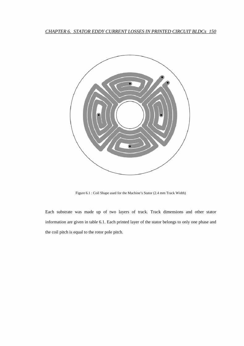
CHAPTER 6. STATOR EDDY CURRENT LOSSES IN PRINTED CIRCUIT BLDCs 150
Figure 6.1 : Coil Shape used for the Machine’s Stator (2.4 mm Track Width)
Each substrate was made up of two layers of track. Track dimensions and other stator
information are given in table 6.1. Each printed layer of the stator belongs to only one phase and
the coil pitch is equal to the rotor pole pitch.

CHAPTER 6. STATOR EDDY CURRENT LOSSES IN PRINTED CIRCUIT BLDCs 151
Table 6.1 : Test Motor Details (inner radius = 8 mm, outer radius = 25 mm)
Track Width
(Base Cu = 35 µm)
[mm]
Stator Axial Thickness
[mm] Comments
1 1.6 Single phase test
1 4.8 Full stator test
2.4 1.6 Single phase test
2.4 3.2 Dual phase test
2.4 4.8 Full stator test
3.7 1.6 Single phase test
3.7 4.8 Full stator test
The presented eddy current modelling method is applicable whether printed circuit layers are
shared among phases or belong to a single phase. In this test motor the two printed layers
making up one phase reside on one substrate. Similarly printed layers belonging to the other two
phases reside on two other separate substrates. The three substrates are nominally identical.
However they are displaced circumferentially so that their magnetic axes are separated by 120
electrical degrees. The printed circuit test motor can be operated as a brushless DC motor or as a
synchronous motor.

CHAPTER 6. STATOR EDDY CURRENT LOSSES IN PRINTED CIRCUIT BLDCs 152
6.3 Eddy Current Modelling
This section presents a formal definition, based on Maxwell laws, of the eddy current problem
being investigated. The simplifying assumptions that were necessary to arrive at a practical
solution to the problem are explained. The mains aspects of the proposed solution procedure are
also presented.
6.3.1 Formulation of the Eddy Current Problem
In general the determination of eddy currents is regarded as a quasi-static problem and requires
the simultaneous solution of three of Maxwell’s equations together with the constitutive
equations for each material within the domain of interest. The equations to be solved are given
below.
curl H=J (6.1)
div B=0 (6.2)
curl E=B
t
∂−∂
(6.3)
B=µH (6.4)
J=Jm+ Je + Ji (6.5)
Je=σE (6.6)
Jm= curl M (6.7)
where:
H is magnetic flux intensity;

CHAPTER 6. STATOR EDDY CURRENT LOSSES IN PRINTED CIRCUIT BLDCs 153
J is current density;
E is the electric field induced within printed tracks;
B is magnet flux density;
Ji is the imposed current density;
Je is the induced current density;
Jm is the magnetisation current density;
µ is magnetic permeability;
σ is electric conductivity; and
M is magnetisation of permanent magnets.
The problem of determining eddy current loss distribution in the stator would be excessively
complex if reasonable simplifying assumptions are not made. The main reasons are the complex
geometries involved and the aspect ratios of important sub-domains such as airgaps and copper
tracks. An important assumption on which the proposed model is based is that the inductive
effect of the eddy currents is insignificant. In other words the induced eddy currents have
practically no effect on the flux density distribution set up by the permanent magnets. In
mathematical terms Je is being removed from the right hand side of equations (6.5) and (6.1)
because the effect of Je on B or H is insignificant compared to that of Jm. Very little flux results
from the induced eddy currents because in general they are restricted to loop within a track
thickness.
Neglecting the inductive effect of eddy currents decouples equation (6.3) from equations (6.1)
and (6.2). This greatly simplifies the problem of determination of eddy current loss distribution
since equations (6.1) and (6.2), together with constitutive relations (6.4) and (6.7), can be solved

CHAPTER 6. STATOR EDDY CURRENT LOSSES IN PRINTED CIRCUIT BLDCs 154
as a magnetostatic problem. The magnetostatic solution can then be used, together with
equations (6.3) and (6.6), to determine the induced current distribution.
6.3.2 Determination of Magnetic Flux Density Distribution
A three dimensional magnetostatic solution for the test machine was arrived at based on the
finite element method (FEM). As shown in figure 6.2, symmetry planes allowed the full 3-D
problem to be reduced and only one sixteenth of the full geometry needed to be considered,
following the same approach adopted in chapter 3.
Figure 6.2 : FEMLAB® Model of the Rotor (Half Pole Pitch, inner Radius of Permanent Magnet = 11 mm)
Y position [m]
Z position [m]
X position [m] 0
0
0.01
0.02
0.03
0
0.01
0.02 0.03
0.05 0.04
0.01 0.02
0.03

CHAPTER 6. STATOR EDDY CURRENT LOSSES IN PRINTED CIRCUIT BLDCs 155
The ironless nature of the stator allowed a single magnetostatic solution to be used for the entire
eddy current evaluation procedure. In other words armature reaction is neglected and the flux
density distribution set up by the permanent magnets is assumed to be undisturbed by rotor
movement or stator currents. Equation (6.8) expresses this assumption mathematically in terms
of spatial co-ordinates r, θ and z.
B(r, θ, z, t) = B(r, θ-ωt, z, 0) (6.8)
where:
B(r, θ, z, t) = flux density seen, at time t, by an observer fixed to the stator at location (r, θ, z)
ω = speed of the rotor in mechanical radians per second
Equation (6.8) is justified by the fact that the stator is ironless. It is also a consequence of the
assumption that flux due to eddy currents is negligible.

CHAPTER 6. STATOR EDDY CURRENT LOSSES IN PRINTED CIRCUIT BLDCs 156
6.3.3 Induced Current Evaluation
It is well-known that if a magnetic field is static and a straight conductor of length 1 metre
moves relative to the magnetic field then the induced electromagnetic force (EMF) across that
conductor is given by:
E = Bzvsin(λ) (6.9)
where:
Bz is the component of flux density that is normal to the plane in which the conductor lies;
v= ωr = relative speed between the magnetic field and the conductor; and
λ is the angle between the conductor and the direction of relative motion.
Equation (6.9) can be used to find the induced voltage around a conducting loop as a result of
relative movement between the conducting loop and a static magnetic field. In order to do this,
the conducting loop should be discretised into sufficiently small elements. Equation (6.9) can
then be applied to each of the elements. The sum of the calculated induced voltages will be equal
to the loop EMF. The loop current flowing as a result of the induced voltage can be assumed to
be equal to the induced voltage divided by the loop resistance. The preceding sentence is based
on the following assumptions:
(a) The induced current does not significantly influence the magnetic field causing the
induced voltage.
(b) The effect of the conducting loop inductance is negligible compared to the effect of its
resistance.
(c) The conducting loop is not electrically connected to anything else.

CHAPTER 6. STATOR EDDY CURRENT LOSSES IN PRINTED CIRCUIT BLDCs 157
The proposed eddy current evaluation procedure is based on the basic idea presented in the
previous paragraph. However, while for the purposes of eddy current evaluation, the stator
printed tracks may be regarded as a large number of conducting loops, those loops are
interconnected which means that assumption (c) above is not valid. It will be shown that, by
application of standard circuit theory to the collection of interconnected loops representing the
stator printed coil, assumption (c) becomes unnecessary.
The validity of assumption (a) relies on the fact that the induced currents are resistively limited.
The eddy currents within the printed copper tracks may, to a first approximation, be assumed to
experience a resistance which is at least twice the resistance seen by normal load currents. Thus
the eddy current path resistance would be of the order of tens of milliohms per metre. Similarly
the inductance of the eddy current paths within a track may be taken to be approximately equal
to the loop inductance of a two-wire transmission line where the two wires are in very close
proximity. Based on this, the eddy current loop inductance would be of the order of one
microhenry per metre. With an estimated eddy current loop time constant of about 0.1
millisecond, the assumption of resistively limited eddy currents would be valid well beyond 15
krpm, which is outside the speed range of the type of machine being considered.
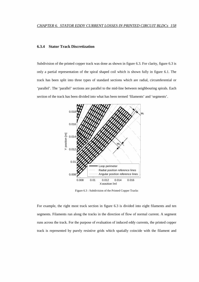
CHAPTER 6. STATOR EDDY CURRENT LOSSES IN PRINTED CIRCUIT BLDCs 158
6.3.4 Stator Track Discretization
Subdivision of the printed copper track was done as shown in figure 6.3. For clarity, figure 6.3 is
only a partial representation of the spiral shaped coil which is shown fully in figure 6.1. The
track has been split into three types of standard sections which are radial, circumferential or
‘parallel’. The ‘parallel’ sections are parallel to the mid-line between neighbouring spirals. Each
section of the track has been divided into what has been termed ‘filaments’ and ‘segments’.
Figure 6.3 : Subdivision of the Printed Copper Tracks
For example, the right most track section in figure 6.3 is divided into eight filaments and ten
segments. Filaments run along the tracks in the direction of flow of normal current. A segment
runs across the track. For the purpose of evaluation of induced eddy currents, the printed copper
track is represented by purely resistive grids which spatially coincide with the filament and
0.008 0.01 0.012 0.014 0.016
0.008
0.01
0.012
0.014
0.016
0.018
X position [m]
Y p
ositi
on [
m]
Loop perimeter
Radial position reference linesAngular position reference lines
ws
wf

CHAPTER 6. STATOR EDDY CURRENT LOSSES IN PRINTED CIRCUIT BLDCs 159
segment boundaries. The resistance of each of the branches forming a grid is determined
according to equations (6.10) and (6.11).
Ria= ws/(σtcwf)= Rea/2 (6.10)
Rib= wf/(σtcws)= Reb/2 (6.11)
where:
Ria= resistance of internal branch along the track;
Rea= resistance of branch along the track on the grid edge;
Rib= resistance of internal branch across the track;
Reb= resistance of branch across the track on the edge of the grid;
ws = width of segment;
wf = width of filament;
tc = track thickness; and
σ= electrical conductivity of track;
As long as the number of filaments and segments are sufficiently large, the replacement of the
actual printed coil by a number of resistive grids is considered to be a reasonable approximation.
As shown in figure 6.3, in the neighbourhood of the edges of the grids there are small sections of
tracks that are not directly represented. However any error arising because of this non-
representation is insignificant because only a relatively small part of the track is involved and for
each non-represented area there is an approximately equal area in the same neighbourhood that
is doubly represented. Node pairs at the edges of adjacent grids are considered to be electrically
connected.

CHAPTER 6. STATOR EDDY CURRENT LOSSES IN PRINTED CIRCUIT BLDCs 160
The model that is being suggested is only a two dimensional representation of the printed circuit
coil. In other words the assumption is that induced current density is uniform within the printed
track in the axial direction. This assumption is justified because:
(a) track thicknesses that are being considered are no greater than 100 µm whereas the track
widths are typically greater than 1 mm;
(b) there is practically no change in the axial component of the flux density due to the
permanent magnet over a distance of 100 µm in the neighbourhood of the printed coil;
and
(c) the highest track thickness that is of interest is much smaller than one skin depth at the
highest relevant eddy current frequency.
The question of sufficiency of number of filaments (nf) and number of segments (ns) needed to
be addressed. Generally higher values of nf and ns leads to better accuracy but at the expense of
higher memory requirement and computation time. One basic requirement is to ensure that nf
and ns are chosen such that both ws and wf are significantly smaller than one skin depth at the
highest eddy current frequency of interest. It has been quite easy to meet this requirement while
staying well under computer memory limitations. Sufficiency of number of filaments and
segments were verified by comparing solutions obtained using nominal values for nf and ns with
those obtained when significantly higher values are used.

CHAPTER 6. STATOR EDDY CURRENT LOSSES IN PRINTED CIRCUIT BLDCs 161
6.3.5 Determination of Eddy Current Loss Distribution
According to the proposed model induced eddy currents within the stator printed tracks are
approximated by currents flowing in the resistive grids of figure 6.3. For clarity, it may be
assumed that the stator winding is open-circuited. The grid currents can be determined by
standard loop analysis which is based on the following matrix equation.
I loop=( Rloop)-1Eloop (6.12)
where:
I loop is the array of loop currents;
Eloop is array of loop EMFs; and
Rloop is the loop resistance matrix
Examples of loops and the adopted loop numbering system are shown in figure 6.4. It is well
known that construction of the loop resistance matrix is based on Kirchhoff’s voltage law.
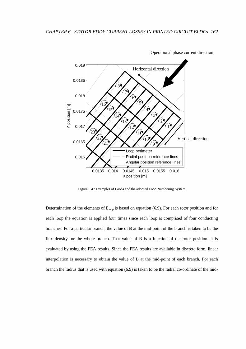
CHAPTER 6. STATOR EDDY CURRENT LOSSES IN PRINTED CIRCUIT BLDCs 162
Figure 6.4 : Examples of Loops and the adopted Loop Numbering System
Determination of the elements of Eloop is based on equation (6.9). For each rotor position and for
each loop the equation is applied four times since each loop is comprised of four conducting
branches. For a particular branch, the value of B at the mid-point of the branch is taken to be the
flux density for the whole branch. That value of B is a function of the rotor position. It is
evaluated by using the FEA results. Since the FEA results are available in discrete form, linear
interpolation is necessary to obtain the value of B at the mid-point of each branch. For each
branch the radius that is used with equation (6.9) is taken to be the radial co-ordinate of the mid-
0.0135 0.014 0.0145 0.015 0.0155 0.016
0.016
0.0165
0.017
0.0175
0.018
0.0185
0.019
X position [m]
Y p
ositi
on [
m]
Loop perimeter
Radial position reference linesAngular position reference lines
10
Operational phase current direction
Horizontal direction
Vertical direction
1 2
3 4
5 6
7 8
11 12
13 14
15 16
9 21 22
23

CHAPTER 6. STATOR EDDY CURRENT LOSSES IN PRINTED CIRCUIT BLDCs 163
point of the branch. Any element of Eloop is the sum of four values calculated using equation
(6.9) taking into consideration the polarity of the calculated EMFs.
For each rotor position Iloop can be determined by using equation (6.10). Branch currents can be
deduced from loop currents by using the loop to branch incidence matrix A. Equation (6.13)
expresses the relationship between loop currents and branch currents. Ibranch is the array of branch
currents.
Ibranch= AI loop (6.13)
The spatial distribution of eddy current loss can be determined by evaluating the resistive loss
for each resistive branch. Summation of the resistive losses of all the branches of the resistive
grids representing a printed coil gives the total eddy current loss for that printed coil.
6.4 Theoretical Predictions
6.4.1 Effect of Track Width and Number of Turns
Figure 6.5 represents calculated eddy current loss for three printed stator substrates that were
made for the test motor of figure 3.6, chapter 3. The three printed stators were nominally
identical in all respects except for the track widths and the number of turns per spiral.

CHAPTER 6. STATOR EDDY CURRENT LOSSES IN PRINTED CIRCUIT BLDCs 164
Figure 6.5 : Calculated Eddy Current Loss for Different Track Widths
(for the Middle Phase at 1000 rpm)
With the widest track of 3.7 mm only 2 turns per spiral are able to be accommodated on the
substrate. The number of turns per spiral for the other two stator substrates were respectively 6
(1 mm track) and 3 (2.4 mm track). As expected the eddy current loss was found to be a strong
function of track width. The induced EMF that drives the eddy current within the active section
of each track is, to a first approximation, proportional to track width. The eddy current loss is
proportional to the square of that induced EMF and inversely proportional to the track resistance.
0 pi/2 pi 3/2*pi 2*pi0
0.01
0.02
0.03
0.04
0.05
0.06
0.07
0.08
0.09
0.1
Actual Position θ [el. rad]
Edd
y C
urre
nts
Loss
[W
]
3.7 mm Track Width
2.4 mm Track Width
1.0 mm Track Width
CHAPTER 6. STATOR EDDY CURRENT LOSSES IN PRINTED CIRCUIT BLDCs 165
Thus a wider track suffers more from eddy currents because its induced EMF is higher and its
resistance is lower.
Figure 6.5 shows that there is variation in the level of eddy current loss as the rotor position
changes. This is specially the case when the number of turns is small. Each turn in the spiral may
be considered to have a component of eddy current loss that is independent of rotor position and
a ripple component. The spatial frequencies present in the ripple component result from the
spatial harmonic frequencies in the air-gap flux density distribution set up by the rotor
permanent magnets. The total eddy current loss for a spiral is the sum of eddy current loss of the
individual turns making up that spiral. The ripple components in the eddy current loss of
individual turns of a spiral may not be in phase and may cancel or partially cancel each other as
a result of summation. These two important statements find their justification in a turn by turn
analysis. All presented cases from 1 mm to 3.7 mm have been analysed turn by turn and results
are presented in figures 6.6 to 6.8. Since the spiral turns have a different pitch, the axial flux
density experienced by every turn is different. In cases where the circumferential displacement
between coil sides is large enough, complete phase reversal of the ripple component appears.
The reversal can clearly be observed in all analysed track widths. In the 3.7 mm case, with only
two turns on the substrate, ripple cancellation is small but still significant. With decreasing track
width, there is a smoother transition, because of the gradual change in position of the spiral
turns. In the 1 mm case this transition is very visible. It is interesting to point out, that in cases
where the turn span is close to half-pitch, the waveform, except for the ripple caused by the
spatial harmonics, is quite flat (for example turn 3 in the 1 mm case or turn 2 in the 2.4 mm
case).
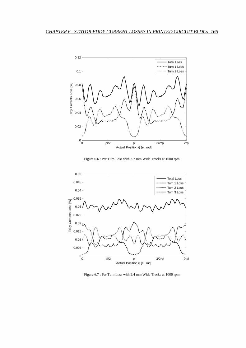
CHAPTER 6. STATOR EDDY CURRENT LOSSES IN PRINTED CIRCUIT BLDCs 166
Figure 6.6 : Per Turn Loss with 3.7 mm Wide Tracks at 1000 rpm
Figure 6.7 : Per Turn Loss with 2.4 mm Wide Tracks at 1000 rpm
0 pi/2 pi 3/2*pi 2*pi0
0.02
0.04
0.06
0.08
0.1
0.12
Actual Position θ [el. rad]
Edd
y C
urre
nts
Loss
[W
]
Total Loss
Turn 1 Loss
Turn 2 Loss
0 pi/2 pi 3/2*pi 2*pi0
0.005
0.01
0.015
0.02
0.025
0.03
0.035
0.04
0.045
0.05
Actual Position θ [el. rad]
Edd
y C
urre
nts
Loss
[W
]
Total Loss
Turn 1 Loss
Turn 2 Loss
Turn 3 Loss

CHAPTER 6. STATOR EDDY CURRENT LOSSES IN PRINTED CIRCUIT BLDCs 167
Figure 6.8 : Per Turn Loss with 1 mm Wide Tracks at 1000 rpm
Summarizing, based on figures 6.5, the ripple in eddy current loss curves is less prominent in the
case of the narrower tracks. There are two reasons for this. Firstly the ripple component of eddy
current losses, just like the rotor position independent component of eddy current losses, is
strongly dependent on track width. Secondly, as illustrated in figure 6.8, a higher number of
turns in a spiral makes cancellation of the ripple components more likely.
0 pi/2 pi 3/2*pi 2*pi0
0.001
0.002
0.003
0.004
0.005
0.006
0.007
0.008
0.009
0.01
Actual Position θ [el. rad]
Edd
y C
urre
nts
Loss
[W
]
Total LossTurn 1 Loss
Turn 2 Loss
Turn 3 Loss
Turn 4 Loss
Turn 5 LossTurn 6 Loss
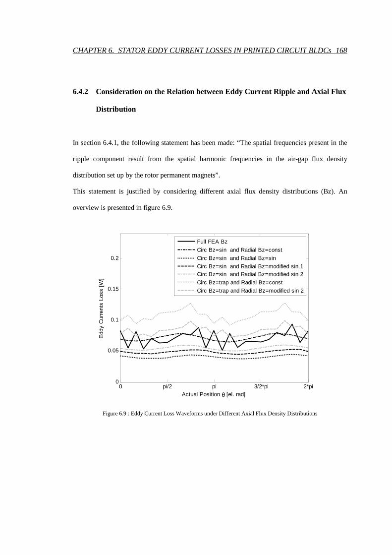
CHAPTER 6. STATOR EDDY CURRENT LOSSES IN PRINTED CIRCUIT BLDCs 168
6.4.2 Consideration on the Relation between Eddy Current Ripple and Axial Flux
Distribution
In section 6.4.1, the following statement has been made: “The spatial frequencies present in the
ripple component result from the spatial harmonic frequencies in the air-gap flux density
distribution set up by the rotor permanent magnets”.
This statement is justified by considering different axial flux density distributions (Bz). An
overview is presented in figure 6.9.
Figure 6.9 : Eddy Current Loss Waveforms under Different Axial Flux Density Distributions
0 pi/2 pi 3/2*pi 2*pi0
0.05
0.1
0.15
0.2
Actual Position θ [el. rad]
Edd
y C
urre
nts
Loss
[W
]
Full FEA Bz
Circ Bz=sin and Radial Bz=const
Circ Bz=sin and Radial Bz=sin
Circ Bz=sin and Radial Bz=modified sin 1Circ Bz=sin and Radial Bz=modified sin 2
Circ Bz=trap and Radial Bz=const
Circ Bz=trap and Radial Bz=modified sin 2

CHAPTER 6. STATOR EDDY CURRENT LOSSES IN PRINTED CIRCUIT BLDCs 169
The model, considering a track width of 3.7 mm and a mechanical speed of 1000 rpm, has been
run with seven different axial flux density distribution (Bz). The first waveform, which
represents the reference, was obtained using Bz resulting directly from FEMLAB®, without any
modifications. For the next four waveforms, Bz is assumed to be sinusoidal in the
circumferential direction. The following four variations in the radial direction have been
considered:
• Bz kept constant from the inner radius towards the outer radius
• Bz varies sinusoidally from the inner radius to the outer radius; the resulting Bz is
presented in figure 6.10.
Figure 6.10 : Bz with Sinusoidal Variation in both Directions.
• Radial Bz varies quasi sinusoidally, since the waveform is slightly flat topped. The
resulting Bz is presented in figure 6.11.
0pi/2
pi3/2*pi
2*pi
00.005
0.010.015
0.020.025
0.03-1
-0.5
0
0.5
1
Rotor Position Θ [electrical radian]Arc-length [m]
Mag
netic
flu
x de
nsity
[T
]

CHAPTER 6. STATOR EDDY CURRENT LOSSES IN PRINTED CIRCUIT BLDCs 170
Figure 6.11 : Bz with modified Sinusoidal (flat topped) Variation in Radial Direction.
• Radial Bz varies approximately similarly to the radial variation of the full Bz resulting
from FEMLAB. The resulting Bz is presented in figure 6.12.
Figure 6.12 : Bz with modified Sinusoidal (approximately as Bz from FEMLAB) Variation in Radial Direction.
0pi/2
pi3/2*pi
2*pi
00.005
0.010.015
0.020.025
0.03-1
-0.5
0
0.5
1
Rotor Position Θ [electrical radian]Arc-length [m]
Mag
netic
flu
x de
nsity
[T
]
0pi/2
pi3/2*pi
2*pi
00.005
0.010.015
0.020.025
0.03-1
-0.5
0
0.5
1
Rotor Position Θ [electrical radian]Arc-length [m]
Mag
netic
flu
x de
nsity
[T
]
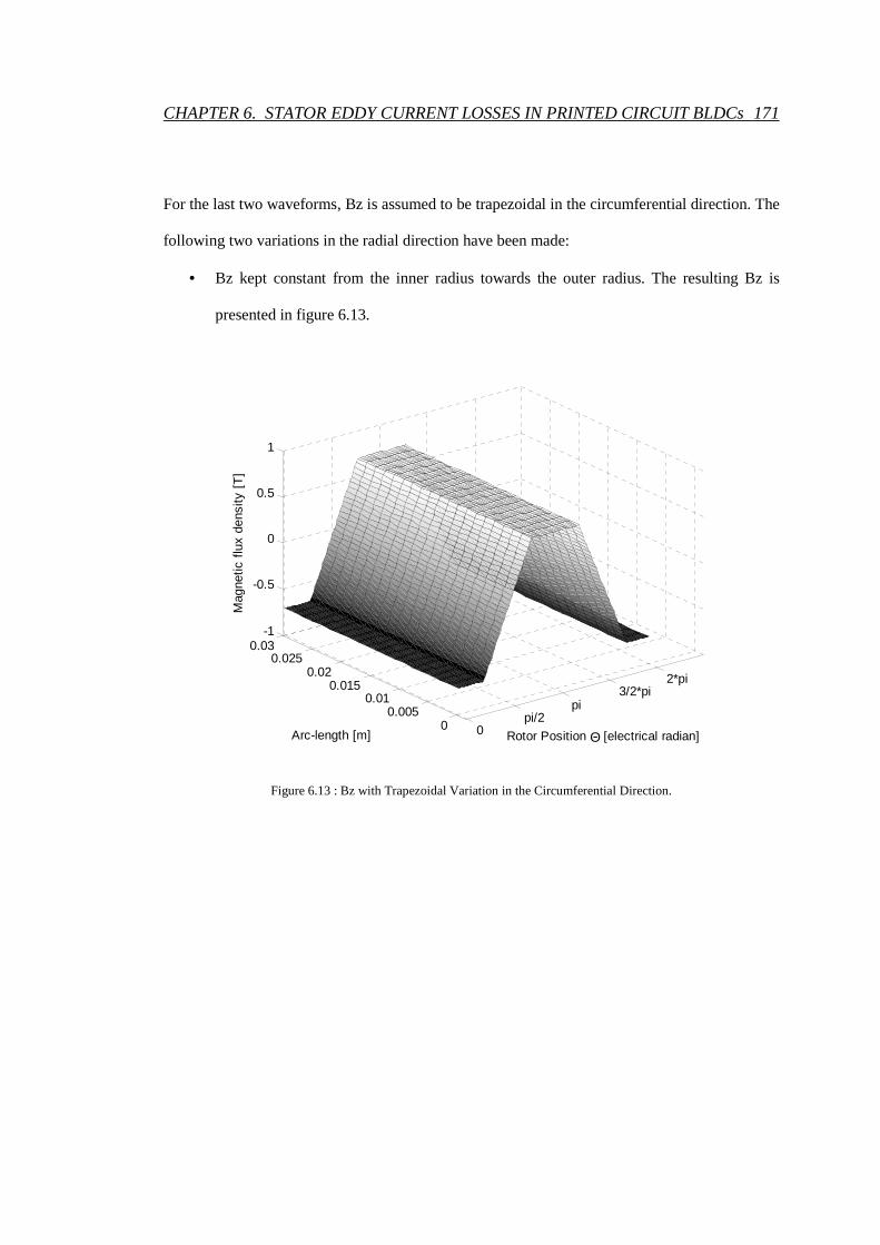
CHAPTER 6. STATOR EDDY CURRENT LOSSES IN PRINTED CIRCUIT BLDCs 171
For the last two waveforms, Bz is assumed to be trapezoidal in the circumferential direction. The
following two variations in the radial direction have been made:
• Bz kept constant from the inner radius towards the outer radius. The resulting Bz is
presented in figure 6.13.
Figure 6.13 : Bz with Trapezoidal Variation in the Circumferential Direction.
0pi/2
pi3/2*pi
2*pi
00.005
0.010.015
0.020.025
0.03-1
-0.5
0
0.5
1
Rotor Position Θ [electrical radian]Arc-length [m]
Mag
netic
flu
x de
nsity
[T
]
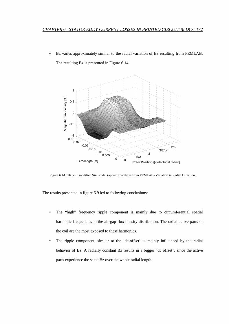
CHAPTER 6. STATOR EDDY CURRENT LOSSES IN PRINTED CIRCUIT BLDCs 172
• Bz varies approximately similar to the radial variation of Bz resulting from FEMLAB.
The resulting Bz is presented in Figure 6.14.
Figure 6.14 : Bz with modified Sinusoidal (approximately as from FEMLAB) Variation in Radial Direction.
The results presented in figure 6.9 led to following conclusions:
• The “high” frequency ripple component is mainly due to circumferential spatial
harmonic frequencies in the air-gap flux density distribution. The radial active parts of
the coil are the most exposed to these harmonics.
• The ripple component, similar to the ‘dc-offset’ is mainly influenced by the radial
behavior of Bz. A radially constant Bz results in a bigger “dc offset”, since the active
parts experience the same Bz over the whole radial length.
0pi/2
pi3/2*pi
2*pi
00.005
0.010.015
0.020.025
0.03-1
-0.5
0
0.5
1
Rotor Position Θ [electrical radian]Arc-length [m]
Mag
netic
flu
x de
nsity
[T
]
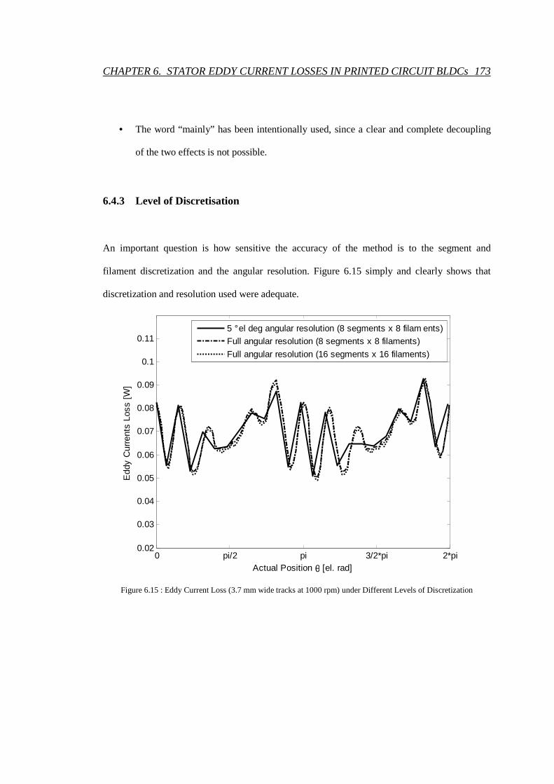
CHAPTER 6. STATOR EDDY CURRENT LOSSES IN PRINTED CIRCUIT BLDCs 173
• The word “mainly” has been intentionally used, since a clear and complete decoupling
of the two effects is not possible.
6.4.3 Level of Discretisation
An important question is how sensitive the accuracy of the method is to the segment and
filament discretization and the angular resolution. Figure 6.15 simply and clearly shows that
discretization and resolution used were adequate.
Figure 6.15 : Eddy Current Loss (3.7 mm wide tracks at 1000 rpm) under Different Levels of Discretization
0 pi/2 pi 3/2*pi 2*pi0.02
0.03
0.04
0.05
0.06
0.07
0.08
0.09
0.1
0.11
Actual Position θ [el. rad]
Edd
y C
urre
nts
Loss
[W
]
5 ° el deg angular resolution (8 segments x 8 filam ents)
Full angular resolution (8 segments x 8 filaments)
Full angular resolution (16 segments x 16 filaments)

CHAPTER 6. STATOR EDDY CURRENT LOSSES IN PRINTED CIRCUIT BLDCs 174
6.4.4 Effect of Substrate Position
Figure 3.6 has shown that the stator of the test machine has its outer phases closer to the rotor
magnets compared to the middle phase. As illustrated in figure 6.16 this gives rise to
significantly higher eddy current losses in the outer phases. The substrates closer to the magnet
are exposed to a higher flux density which gives rise to higher induced EMFs. Even a small
difference in induced EMF leads to a relatively large difference in eddy current loss because the
loss is a function of the square of the induced EMF.
Figure 6.16 : Calculated Eddy Current Loss for different Phases (at 1000 rpm)
0 pi/2 pi 3/2*pi 2*pi0
0.01
0.02
0.03
0.04
0.05
0.06
Actual Position θ [el. rad]
Edd
y C
urre
nts
Loss
[W
]
Top Phase 2.4 mm Track Width
Middle Phase 2.4 mm Track Width

CHAPTER 6. STATOR EDDY CURRENT LOSSES IN PRINTED CIRCUIT BLDCs 175
6.4.5 Eddy Current Paths
This section focuses on spatial distribution of the induced eddy currents. Before going into
details definition of directions have to be made. Figure 6.17 presents the reference directions.
The arrow is always taken as reference in order to define positive / negative horizontal and
vertical currents, but it does not represent any eddy current path.
-0.015 -0.01 -0.005 0 0.005 0.01 0.0150.006
0.008
0.01
0.012
0.014
0.016
0.018
0.02
0.022
0.024
X position [m]
Y p
ositi
on [
m]
Loop perimeter
Figure 6.17 : Direction Definitions
Figures 6.18 and 6.20 present the eddy currents inside the spiral at two different rotor positions.
The line width of each “branch-line” (horizontal and vertical) depends on the amplitude of the

CHAPTER 6. STATOR EDDY CURRENT LOSSES IN PRINTED CIRCUIT BLDCs 176
eddy current flowing in this particular branch. The color of the “branch-line” depends on the
sign of the eddy current: dark-gray represents positive currents, light-grey negative ones.
Figure 6.18 : Eddy Current Distribution at Position 0° (both rotor and stator axis are aligned)
To avoid misinterpretation of figures 6.18 and 6.20, it is important to present details on the
boundaries, where the track changes from radial to circumferential. At first it could appear that
there is break in the eddy current paths. That is not the case (would not be possible from an
electrical point of view). This is only due to the adopted geometric model. Figure 6.19 presents
how the broken lines are ‘mathematically’ connected. This connection is depicted by the dashed
lines.
-0.015 -0.01 -0.005 0 0.005 0.01 0.0150.006
0.008
0.01
0.012
0.014
0.016
0.018
0.02
0.022
0.024

CHAPTER 6. STATOR EDDY CURRENT LOSSES IN PRINTED CIRCUIT BLDCs 177
Figure 6.19 : Tracks Boundaries between Different Sections
Figures 6.18 and 6.20 clearly show how the eddy currents flow in “concentric loops” and mainly
in “vertical” direction. There are also horizontal currents, mainly where the loops “end” (they are
like “end-part connections” for the concentric loops). It is interesting to observe that a portion of
the “arc”-sections can be part of the “concentric loops”, since there is no insulation and the eddy
currents will flow there to “close” the loop. At this point it is important to mention, that eddy
currents can also be induced in the arc sections, since two of the four loop edges (discretization
loops) are still in the “active” direction. This can be seen in figure 6.20, where stator coil axis is
aligned with rotor q-axis.

CHAPTER 6. STATOR EDDY CURRENT LOSSES IN PRINTED CIRCUIT BLDCs 178
Figure 6.20 : Eddy Current Distribution at Position 90° electrical Degrees
6.4.6 Co-existence of Eddy and Load Currents
In practice the eddy currents induced in the printed coils will be superimposed onto normal load
current flowing in those coils. An important question is whether this co-existence leads to
additional losses. In order to analyse this question it is assumed that the normal load current
flows through the grid branches totally along the printed track and not though the grid branches
across the track. This means that if R is the resistance of a track section, I is the motor current
and Ie is the eddy current then total resistive loss, to a first approximation, is given by:
2(I/2+Ie)2R+2(I/2- Ie)
2R = I2R + 4(Ie)2R = loss due to normal current+eddy current loss (6.14)
-0.015 -0.01 -0.005 0 0.005 0.01 0.0150.006
0.008
0.01
0.012
0.014
0.016
0.018
0.02
0.022
0.024

CHAPTER 6. STATOR EDDY CURRENT LOSSES IN PRINTED CIRCUIT BLDCs 179
Equation (6.14) predicts that the co-existence of normal machine currents and induced eddy
currents within printed tracks does not cause additional losses.
In practice eddy currents will be induced simultaneously in all phases of the motor. As shown in
figure 6.21, the eddy current loss for the stator is the sum of the eddy current loss of the three
individual substrates. As expected this summation results in significant reduction in the ripple
content of the eddy current losses. Indeed if the number of turns is high enough total eddy
current losses can be assumed to be independent of rotor position.
Figure 6.21 : Calculated Eddy Current Loss for Different Track Widths (full 3 Phase Machine at 1000 rpm)
0 pi/2 pi 3/2*pi 2*pi0
0.05
0.1
0.15
0.2
0.25
0.3
0.35
Actual Position θ [el. rad]
Edd
y C
urre
nts
Loss
[W
]
3.7 mm Full Machine Loss
2.4 mm Full Machine Loss
1.0 mm Full Machine Loss

CHAPTER 6. STATOR EDDY CURRENT LOSSES IN PRINTED CIRCUIT BLDCs 180
6.5 Experimental Validation
The method of experimental validation is based on the fact that it is mechanical energy coming
from the rotor that gets converted to eddy current losses. The preceding statement remains true
irrespective of whether the brushless printed circuit machine operates as a motor or as a
generator. For convenience tests were performed with the machine running as a generator.
a)
b)
Figure 6.22 : a) Ceramic Bearing for Stator Support; b) Arrangement for Force Measurement
Motor Shaft (coupled with the driving motor)
Scale Base Plate
Rotor disk
Torque Arm
Substrates Stack
Permanent Magnet
Motor Shaft (coupled with the driving motor)
Permanent Magnet
Rotor Disk
Ceramic Bearing (with shoulder to hold the
substrates stack)

CHAPTER 6. STATOR EDDY CURRENT LOSSES IN PRINTED CIRCUIT BLDCs 181
The arrangement illustrated in figure 6.22 (b) was used to carry out specially designed tests. The
printed circuit machine under test was motor driven. The stator of the machine was bearing
mounted (figure 6.22 (a)) onto the shaft effectively allowing the overall system to operate as a
dynamometer. As shown in figure 6.22 a torque arm attached to the stator was made to rest on an
electronic scale which had a resolution of 0.1 gram. The length of the torque arm was 0.050 m.
An eddy current loss of Pe watts requires a rotor driving torque of Te which is given by Pe/ω
where ω is the rotor speed. This torque is measurable on the electronic scale as a force given by:
Fe = Pe/(Laω) (6.15)
where La is the length of the torque arm.
Assuming that the stator is open circuited, the actual measurement on the electronic scale will be
due to a combination of bearing friction torque (FrLa) and the driving torque needed to generate
the eddy currents. Special low friction ceramic bearings were used to mount the stator onto the
shaft. Pre-tests were performed on the bearing to determine Fr at 1000 rpm and at 1600 rpm.
The pre-tests were performed with the bearing mounted on the shaft without the stator and with
the torque arm mounted on the outer race of the bearing. Subsequent tests on a number of
different stators were performed at 1000 rpm and at 1600 rpm. It was assumed that Fr remains
constant if speed remains constant. Fe was taken to be the difference between the reading on the
electronic weighing scale and Fr whose value was 1.1 gram at 1000 rpm and 1.3 gram at 1600
rpm.

CHAPTER 6. STATOR EDDY CURRENT LOSSES IN PRINTED CIRCUIT BLDCs 182
Table 6.2 shows good agreement between measured values of Fe and those predicted using the
method described in section 6.4. The percentage discrepancy is less than 6% for the two wider
tracks. For the 1 mm track the error is larger because the force being measured falls within the
resolution of the electronic scale.
Table 6.2 : Force Measurements width Different Track Widths (Base Cu = 35 µm)
Track Width [mm]
Speed [rpm]
Middle Phase Full stator
Measured [g]
Simulated [g]
Error [%]
Measured [g]
Simulated [g]
Error [%]
3.7 1000 1.4 1.363 2.64 5.2 5.097 1.98
1600 2.3 2.181 5.17 8.4 8.155 2.92
2.4 1000 0.6 0.597 0.50 2.3 2.270 1.30
1600 1.0 0.955 4.50 3.8 3.632 4.42
1.0 1000 0.1 0.096 4.00 0.4 0.368 8.00
1600 0.2 0.153 23.50 0.6 0.588 2.00
Additional tests were performed to confirm the validity of equation (6.14) which states that co-
existence of eddy-currents and normal operating currents does not result in increased stator loss
beyond the sum of the separately calculated losses. Those tests were performed with the printed
circuit machine running as a resistively loaded generator. Prediction for instantaneous phase
EMFs was based on equation (6.9). From instantaneous phase EMFs, average power consumed
by the resistive loads was evaluated and converted to an equivalent braking force as presented in
figure 6.23. Table 6.3 shows that there is reasonable agreement between the measured total
braking Ft and total force that was predicted using equation (6.14). The fundamental reason for

CHAPTER 6. STATOR EDDY CURRENT LOSSES IN PRINTED CIRCUIT BLDCs 183
insignificant additional loss due to co-existence of eddy-currents and load current is the small
ratio of width to length of the copper tracks.
Table 6.3 : Force Measurements (two substrates mounted, 2.4 mm track width)
Speed [rpm]
Load Resistance not Connected Load Resistance (0.66 ohm) Connected
Measured [g]
Predicted [g]
Error [%]
Measured [g]
Predicted [g]
Error [%]
1000 1.5 1.433 4.47 8.3 8.034 3.25
1600 2.3 2.292 0.35 13.3 12.854 3.38
Figure 6.23 : Braking Force of the Middle and Top Phase at 1000 rpm
0 pi/2 pi 3/2*pi 2*pi0
1
2
3
4
5
6
7
Actual Position θ [el. rad]
For
ce [
g]
Top Phase
Middle Phase

CHAPTER 6. STATOR EDDY CURRENT LOSSES IN PRINTED CIRCUIT BLDCs 184
6.6 Comparison between I2R and Eddy Current Loss
As for the optimization algorithm introduced in chapter 3, the phase EMF at a nominally fixed
mechanical speed of 1000 rpm + / - 10% has been chosen as reference, in order to make
meaningful comparisons. The axial length of the permanent magnet has been adapted for all
cases in order to have exactly the same axial flux density in the stator air gap. The assumed
phase current is 1 A.
1 mm track width (6 turns)
Phase I2R Losses = 1.22W
Phase Eddy Current Loss = 0.0048 W
Ratio= Eddy Loss / I2R = 0.39 %
2.4 mm track width (3 turns)
Phase I2R Losses = 0.5484W
Phase Eddy Current Loss = 0.060W
Ratio = Eddy Loss / I2R= 10.94 %
3.7 mm track width (2 turns)
Phase I2R Losses = 0.3027W
Phase Eddy Current Loss = 0.208W
Ratio= Eddy Loss / I2R= 68.71 %

CHAPTER 6. STATOR EDDY CURRENT LOSSES IN PRINTED CIRCUIT BLDCs 185
From the above, it is clear that eddy current loss rises sharply with track width. Every
application should be considered on its own merit when a decision on maximum track width is
being made. Eddy current loss becomes an increasingly important consideration as speed
increases. For the purpose of this thesis, as specified in table 3.2, track width was limited to
2.5mm.
6.7 Conclusion
During normal operation of a motor with a printed circuit stator, eddy currents are induced
within the stator tracks. The significance of such currents depends mainly on speed and on the
track width. A computationally efficient numerical method has been developed to evaluate eddy
current losses within the stators of printed circuit brushless motors. The theoretical basis of the
proposed technique has been presented. The technique has been experimentally validated by
specially designed tests. It was found stator eddy current loss is independent of the flow of
normal stator current.
186
Chapter 7
Prediction of Inductances of Printed
Circuit Motors
7
7.1 Introduction
The variation of stator inductances with rotor position plays a crucial role in BLDC motor
commutation control systems that are based on the equal inductance method. If a BLDC motor is
being designed and the intention is to use the equal inductance method for sensorless
commutation of that motor, then there is a need to ensure right at the design stage that the motor
will have sufficient inductive saliency. While prototypes could be built and tested to determine
inductances, it is much more economical and convenient to carry out theoretical predictions.
However, the method of prediction should be accurate, easy to use and cost effective. This

CHAPTER 7. PREDICTION OF IND. OF PRINTED CIRCUIT MOTORS 187
chapter is about the development of such a method. The requirement for relatively high accuracy
ruled out purely analytical methods. Consequently the adopted method was numerical. In this
chapter the theoretical basis behind the method is explained and test results are presented which
confirm its validity.
Stator inductance may also be required to estimate the size of current ripple at a particular PWM
frequency. For this purpose, a first order estimation may be sufficient. A closed form formula for
first order estimation of the stator inductance is given in appendix C.
7.2 Basic Principles
By definition the self inductance of a circuit is equal to the flux linking that circuit per ampere of
current flowing through it with all other circuits, to which it is magnetically coupled, open-
circuited. At first the impossibility of open-circuiting eddy current loops within the permanent
magnets and the rotor iron appears to be a difficulty. But this is conveniently resolved by an
alternative, but more appropriate, definition of stator self inductance. The inductance of a
particular stator phase is defined, at a particular frequency, as flux linkage per ampere of
sinusoidal current flowing through that phase with the other two phases open-circuited. This
definition is appropriate for the application being looked at because the self-inductance
evaluated or measured is based on flux distribution that closely resembles the one which would
exist under normal operating conditions. The selected frequency is taken to be the PWM
frequency that the BLDC motor drive would use.

CHAPTER 7. PREDICTION OF IND. OF PRINTED CIRCUIT MOTORS 188
Based on the above definition, the requirement for inductance calculation would be knowledge
of the flux distribution in the BLDC motor when sinusoidal current flows in one of its phase
windings. That flux distribution is influenced by eddy currents flowing in the magnets as well as
in the rotor. Therefore the quasi static solution to Maxwell’s equations is required. Due to the
complexity of the geometry an analytical solution is not possible. A number of numerical
techniques have been developed to solve the quasi-static form of Maxwell’s equations. These
include the finite element method (FEM), the finite difference time domain method, the coupled
network method and the assumed flux path method. Each of those methods has advantages and
disadvantages. For example the FEM has the advantage of giving accurate results, but it requires
expensive software that can be hard to use and computation times can be long. The assumed flux
path method is good as a first approximation, it is computer resource efficient and processing
time is small. Its main disadvantages are that customised software has to be written for each
problem and that good prior knowledge of the main flux paths is necessary. The technique being
used is a combination the assumed flux path method and the coupled network method.
A number of simplifications were necessary to arrive at a solution that is satisfactory in terms of
computer resource requirements, processing time, software development effort and accuracy.
The actual geometry of the problem is represented in figure 7.1. The main difficulty is the three
dimensional nature of the problem. It has been possible to reduce the actual problem to what is
effectively a two dimensional problem by making three reasonable assumptions. These are:
(a) The stator coils which are in reality spirals, as shown in figure 7.2(a), have been
replaced by a number of separate turns, as shown in figure 7.2(b).

CHAPTER 7. PREDICTION OF IND. OF PRINTED CIRCUIT MOTORS 189
(b) Throughout the region of interest the magnetic flux density component along the
direction of the conductors shown in figure 7.2(b) is equal to zero.
(c) Phase inductances are made up of an offset component and a sinusoidal component with
extrema at locations where the magnetic axis of the phase winding aligns with the rotor
direct and quadrature axes.
Figure 7.1 : Overall Problem Geometry
Rotor disks
Permanent Magnets
Y position [m]
0.01
0
-0.01
-0.02
-0.03
0.02 0
0.01
0.02
-0.01
-0.02
0
0.02
-0.02
Shaft Substrates
Z position [m]
X position [m]

CHAPTER 7. PREDICTION OF IND. OF PRINTED CIRCUIT MOTORS 190
As a consequence of the last assumption the inductance at any rotor position may be deduced
from two inductance values evaluated at two different rotor positions. The chosen rotor
positions for inductance evaluation give the direct axis inductances and the quadrature axis
inductances.
7.3 Prediction of Direct Axis Inductances
7.3.1 The Coupled Network Model
As shown in figure 7.2(b), the phase winding has been replaced by a set of infinitely thin
conductors.
a)
-0.015 -0.01 -0.005 0 0.005 0.01 0.015
0.005
0.01
0.015
0.02
0.025
[m]
[m]

CHAPTER 7. PREDICTION OF IND. OF PRINTED CIRCUIT MOTORS 191
b)
Figure 7.2(a) : Actual Spiral, (b): Current Loop Approximation
The coupled network method is essentially about replacing a physical electromagnetic structure
by a reluctive network which is mutually coupled with a resistive network. In general the
reluctive network is made up of a set of nodes with reluctive branches connecting neighbouring
nodes. The diagram in figure 7.3 includes a layer of magnetic nodes that are just above the
conductors representing the stator coils. There are layers of nodes in equally spaced planes
parallel to the coil plane. In particular there is a plane of nodes just below the plane of the stator
coil. Every plane has the same number of nodes and the nodes line up in the axial direction. Note
that there are no magnetic nodes on the plane of the coil.
-0.015 -0.01 -0.005 0 0.005 0.01 0.015
0.005
0.01
0.015
0.02
0.025
[m]
[m]
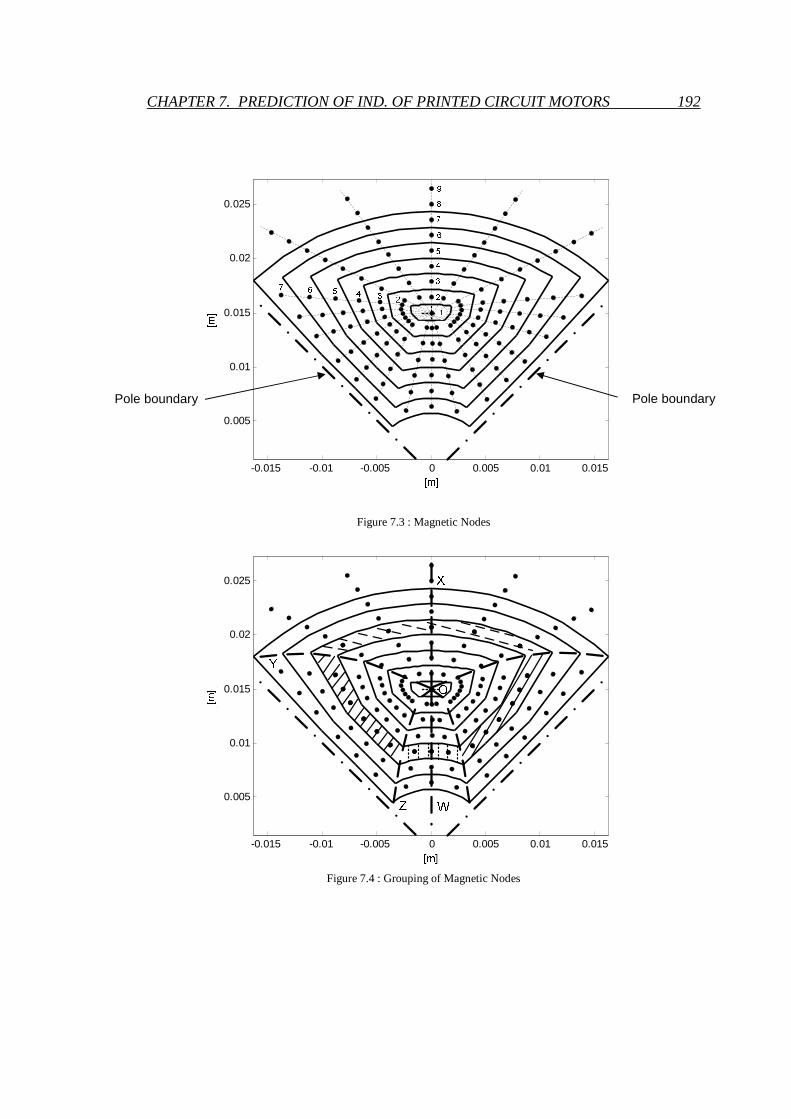
CHAPTER 7. PREDICTION OF IND. OF PRINTED CIRCUIT MOTORS 192
-0.015 -0.01 -0.005 0 0.005 0.01 0.015
0.005
0.01
0.015
0.02
0.025
[mm]
[mm
]
Figure 7.3 : Magnetic Nodes
-0.015 -0.01 -0.005 0 0.005 0.01 0.015
0.005
0.01
0.015
0.02
0.025
[mm]
[mm
]
Figure 7.4 : Grouping of Magnetic Nodes
Pole boundary Pole boundary
CHAPTER 7. PREDICTION OF IND. OF PRINTED CIRCUIT MOTORS 193
Assumption (b) in section 7.2 states that there is zero flux along branches between neighbouring
nodes that lie between two conductors and that fall in the same plane. For example there is no
flux in the branches joining neighbouring pairs of the nodes that are shown in the shaded area of
figure 7.4. This means that those nodes are at the same magnetic potential and therefore they can
be joined together to form single nodes. As shown in figure 7.5, the nodes have been joined to
form three planar networks. In section 7.3.1, it is shown that the use of three networks rather
than a single one allows flexibility in setting realistic boundary conditions. All the nodes
between 0W and 0Z in figure 7.4 have been joined appropriately to form the planar network in
figure 7.5(a). For example all nodes between those lines have been joined to form nodes a1, a2,
a3, a4, a5, a6 and a7.

CHAPTER 7. PREDICTION OF IND. OF PRINTED CIRCUIT MOTORS 194
Figure 7.5(a) : Planar Reluctive Network
Similarly all nodes shown between 0Z and 0Y in figure 7.4 have been joined to form the planar
network in figure 7.5(b).

CHAPTER 7. PREDICTION OF IND. OF PRINTED CIRCUIT MOTORS 195
Figure 7.5(b) : Planar Reluctive Network
For example all nodes between those lines have been joined to form nodes b1, b2, b3, b4, b5, b6
and b7 in the planar network of figure 7.5(b).

CHAPTER 7. PREDICTION OF IND. OF PRINTED CIRCUIT MOTORS 196
All nodes between 0Y and 0X in figure 7.4 have been joined appropriately to form the planar
network in figure 7.5(c).
Figure 7.5(c) : Planar Reluctive Network

CHAPTER 7. PREDICTION OF IND. OF PRINTED CIRCUIT MOTORS 197
It has been assumed that electric currents, whether imposed or induced, flow only in planes
parallel to the stator coil plane. Electric circuits link the magnetic network as shown in figures
7.3 and 7.5. Both imposed and induced currents are represented in figure 7.5. The imposed
current is the current flowing through one phase of the stator, the other two phase windings
being open circuited. Currents are induced in the magnets and in the rotor iron.
7.3.2 Branch Reluctance and Loop Resistances
The reluctance in the axial direction Rz up to the outer edge of the rotor iron, is given by:
zz
z
LR
Aµ= (7.1)
where:
Lz = axial separation (defined in figure 7.5)
Az = area between conductor loops (as defined for each network in figure 7.4)
µ = permeability of material
The reluctance in the radial direction Rr , is given by
rr
r
LR
Aµ= (7.2)
where:
Lr = mean separation between inter-conductors mid-lines as shown in figure 7.6
Ar = (conductor perimeter) x ( axial separation)

CHAPTER 7. PREDICTION OF IND. OF PRINTED CIRCUIT MOTORS 198
-6 -4 -2 0 2 4 6
x 10-3
0.011
0.012
0.013
0.014
0.015
0.016
0.017
0.018
0.019
[mm]
[mm
]
Figure 7.6 : Definition of ‘radial’ Length Lr
Note:
a) The same formulae are used for calculation of reluctances in the stator region, air-gap
region, magnet region or iron region. For the first three regions a relative permeability of one
was used. For the iron region the value of permeability was based on flux density
distribution in the iron due to the magnets. The flux density distribution was obtained from a
3-D non-linear magnetostatic solution generated by FEA.
b) Equations similar to (7.1) and (7.3) were used for branch reluctances of network 7.5(c)
which fall in the region beyond the outer radius of the machine.
The resistance of the stator current loops are not required because stator currents are imposed
currents. Resistance values are required for the loops representing eddy current paths in the

CHAPTER 7. PREDICTION OF IND. OF PRINTED CIRCUIT MOTORS 199
magnet and in the rotor iron. As shown in figure 7.5, the magnet and the rotor iron are sliced in
layers parallel to the stator coil. Each layer has its own set of current loops. Figure 7.7 shows the
magnet profile superimposed on the stator conductor loops. For all the magnet and rotor iron
conducting loops except for the outermost ones in the magnet,
conductor
r z
perimeterR
L Lσ= (7.3)
where:
σ = conductivity of the magnet.
The outermost eddy current loop has a perimeter that is equal to the average of the perimeter of
the stator conductor that falls fully within the magnet profile and the perimeter of the magnet.
Equation (7.3) is still used to calculate the resistance of the loop but with cross-sectional area
equal to Lz times the average of Lx. As shown in figure 7.7, Lx is the weighted average of all
discrete distances between the last stator conductor that falls fully within the magnet profile and
the edge of the magnet.

CHAPTER 7. PREDICTION OF IND. OF PRINTED CIRCUIT MOTORS 200
-0.015 -0.01 -0.005 0 0.005 0.01 0.015
0.005
0.01
0.015
0.02
0.025
[mm]
[mm
]
Figure 7.7 : Calculation of Eddy Current Loop Resistances
7.3.3 Boundary Conditions
At the centre of the spiral it is assumed that the flux density is purely axial. Hence, as shown the
right hand side in figure 7.5, a zero flux or magnetic insulation condition is assumed. The left
hand side of figure 5(a) and 5(b) corresponds to the outer periphery of the stator coil. The
reluctive branches on that side represents magnetic paths back to the magnetic zero potential
plane which is the plane separating neighbouring stator coils or neighbouring rotor magnets.

CHAPTER 7. PREDICTION OF IND. OF PRINTED CIRCUIT MOTORS 201
That plane also contains the quadrature axis. In calculating the reluctance of those branches
equation 7.2 has been used. The radial lengths were arrived at as follows:
a) For network b), a weighted average ‘radial’ distance has been used as shown in figure 7.8
b) For network c), the radial length was assumed to be made up of two sections as shown in
figure 7.8
-0.015 -0.01 -0.005 0 0.005 0.01 0.015
0.005
0.01
0.015
0.02
0.025
[mm]
[mm
][m
]
Figure 7.8 : Calculation of radial Distance at Boundary

CHAPTER 7. PREDICTION OF IND. OF PRINTED CIRCUIT MOTORS 202
The left hand side of figure 7.5(c) represents the boundary conditions at the outer arc shown in
figure 7.3.
The network in figure 7.5(c) was extended sufficiently enough in the radial direction so that it
did not matter whether the adopted boundary condition at the radial boundary was a magnetic
short-circuit or a magnetic open-circuit.
7.3.4 Magnetic Circuit Loop Analysis
Ampère’s Law states that:
Hdl enclosed current=∫ (7.4)
The above equation is analogous to Kirchhoff’s voltage law for electric circuits. It states that the
summation of magnetic potential drops around a loop in a magnetic network is equal to the
current enclosed by that loop.
Magnetic potential drop = Reluctance x Branch Flux (7.5)
Branch flux is related to loop flux in exactly the same way that branch currents and loop currents
in an electrical circuit are related to each other. Examples of flux loops are given in figure 7.9.
Magnetic loop analysis results in the following matrix equation:
aa ab ac ad a a
ba bb bc bd b b
ca cb cc cd c c
da db dc dd d d
M M M M I
M M M M I
M M M M I
M M M M I
φφφφ
=
(7.6)
or M Iφ =

CHAPTER 7. PREDICTION OF IND. OF PRINTED CIRCUIT MOTORS 203
where:
Maa, Mbb, Mac, …, Mcb and Mcc are n x n submatrices
Mad, Mbd, Mcd are n x m submatrices
Mda, Mdb, Mdc are m x n submatrices
Mdd is m x m matrix
, , a b cφ φ φ are n x 1 loop flux vectors
dφ is an m x 1 loop flux vectors
Ia, Ib, Ic are n x 1 imposed current vectors
Id is an m x 1 imposed current vector
M is an (n+m) x (n+m) matrix
n, equal to nr x nl is the number of loops in network 5(a) or 5(b), made up of nr loops in the radial
direction and nl loops in the axial direction.
(n+m), equal to (nr + mr) x nl, is the number of loops in network 5(c).
TT T T Ta b c dφ φ φ φ φ =
TT T T Ta b c dI I I I I =
The loop flux vectors are unknowns that need to be determined. The imposed currents are
assumed to be known. The real part of the diagonal elements of Maa, Mbb, Mcc and Mdd is equal to
the sum of reluctances around the loop corresponding to that element. The imaginary part of the
diagonal elements of Maa, Mbb and Mcc is equal to j
R
ωwhere R is the loop resistance calculated
using equation 7.3. If a magnetic loop is not linked by an induced current loop, the
corresponding diagonal entry for this loop will have an imaginary part equal to zero. For

CHAPTER 7. PREDICTION OF IND. OF PRINTED CIRCUIT MOTORS 204
example the diagonal matrix entry for loop x in figure 7.9 is (Rm1 + Rm2 + Rm3 + Rm4 + x
j
R
ω)
whereas the diagonal entry for loop y is (Rm5 + Rm6 + Rm7 + Rm4). The imaginary part of the
diagonals elements of Mdd is equal to zero.
Each off-diagonal element of Maa, Mbb, Mcc and Mdd is a function of the spatial relation between
the two corresponding loops. If the two loops are neighbours then the corresponding matrix
entry is equal to –Rm where Rm is the branch reluctance common to the two loops. If the two
loops are not neighbours then the corresponding matrix entry is equal to zero.
1φ
2φ
3φ
4φ
3mφ
Figure 7.9 : Example of Loop Equations

CHAPTER 7. PREDICTION OF IND. OF PRINTED CIRCUIT MOTORS 205
For example for loop x and loop y the corresponding matrix entry is –Rm4. For loop y and loop z
the corresponding matrix is zero.
The loops have been numbered so that the imaginary part of Maa(i,i) is equal to the imaginary
part of Mbb(i,i) and Mcc(i,i). The real parts of all entries of Mab, Mac, Mba, Mbc, Mca and Mcb are
equal to zero. The imaginary part of Mab(i,i), Mac(i,i), Mba(i,i), Mbc(i,i), Mca(i,i), Mcb(i,i) are all
equal to the imaginary part of Maa(i,i). All entries of Mad, Mbd, Mcd, Mda, Mdb, Mdc are equal to
zero.
For a magnetic loop that is not linked by an imposed current, the corresponding entry in the
imposed current vector will be zero. For example for loop x in figure 7.9, the entry in the
imposed current vector will be zero, whereas for loop u it will be equal to Iu. In equation 7.6:
Ia(i)=Ib(i)=Ic(i).
All the entries of Id are equal to zero.
From equation 7.6 we have:
1
a
b
c
d
M I
φφ
φφφ
−
= =
(7.7)
Once loop fluxes have been obtained from equation 7.7, branch flux, if needed can be easily
deduced. From example branch flux 3mφ in figure 7.9 is equal to ( )1 3φ φ− .
By definition inductance is equal to the flux linkage per ampere. All imposed currents in the
model of figure 7.5 are equal to 1 A. Therefore:
Coil inductance = T Iφ (7.8)

CHAPTER 7. PREDICTION OF IND. OF PRINTED CIRCUIT MOTORS 206
Phase inductance = Number of coils x coil inductance x coupling factor (7.9)
The value of the coupling factor is 0.96. This value was found empirically. It represents the
magnetic coupling between co-axial spirals on different layers of the printed circuit. This
coupling factor may be considered constant for a wide range of stator design.
7.4 Prediction of Quadrature Inductances
Figure 7.10 gives a set of self-inductance measurements made on a prototype machine. All
measurements were carried out at 20 kHz with the rotor at standstill.
Figure 7.10 : Self Inductance Measurements carried out at 20 kHz with Different Machine Configurations
6.5
7
7.5
8
8.5
Sel
f In
duct
ance
s [ µ
H]
Full Machine without PM
Full Machine @ Q-Axis
Wood Rotor Disk (PM mounted) @ Q-AxisSubstrate in free space
Wood Rotor Disk (PM mounted) @ D-Axis
Full Machine @ D-Axis

CHAPTER 7. PREDICTION OF IND. OF PRINTED CIRCUIT MOTORS 207
Two of those measurements were carried out with the iron rotor replaced by a wooden rotor. The
normal q-axis inductance (with iron rotors) and the machine inductance without permanent
magnets (but with iron rotors) are respectively 8.03 µH and 8.25 µH. These values illustrate that
the presence of the permanent magnet has relatively less effect on the q-axis phase inductance.
The reason for this is the air-gap between neighbouring magnets. While the magnets still form
part of eddy current loops, there are no current loops that are totally within magnets as in the
case when stator coils are directly aligned with the rotor direct axis. As shown in figure 7.11 an
eddy current loop section that is through a magnet is connected to the rest of the loop, which is
within a neighbouring magnet, by loop sections within the rotor iron. The current flowing in
loops such as the one shown in figure 7.11 tends to be small compared with the current that
would flow in a loop that is totally within a permanent magnet. The reason for this is the high
resistance of the loop sections within the iron. Resistance in the iron is higher because of the skin
effect. Figure 7.12 illustrates the coupled network model that has been used to evaluate q-axis
inductances. The model is technically the same as the one used for the d-axis model as shown in
figure 7.5. The same solution procedure was followed. The conductive effect of the magnet was
transferred to the current paths representing eddy currents in the rotor.
Figure 7.11 : Q-Axis Eddy Current Paths (for graphical clarity only two loops show)
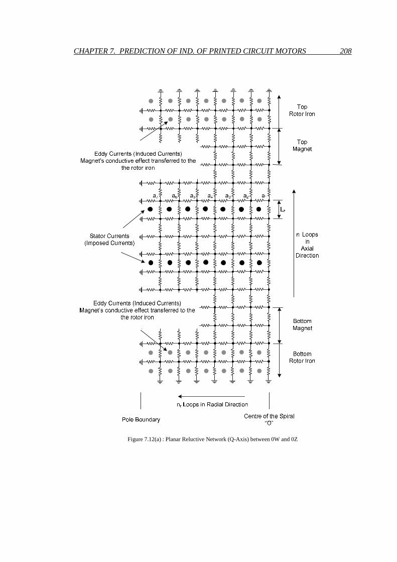
CHAPTER 7. PREDICTION OF IND. OF PRINTED CIRCUIT MOTORS 208
Figure 7.12(a) : Planar Reluctive Network (Q-Axis) between 0W and 0Z

CHAPTER 7. PREDICTION OF IND. OF PRINTED CIRCUIT MOTORS 209
Figure 7.12(b) : Planar Reluctive Network (Q-Axis) between 0Z and 0Y
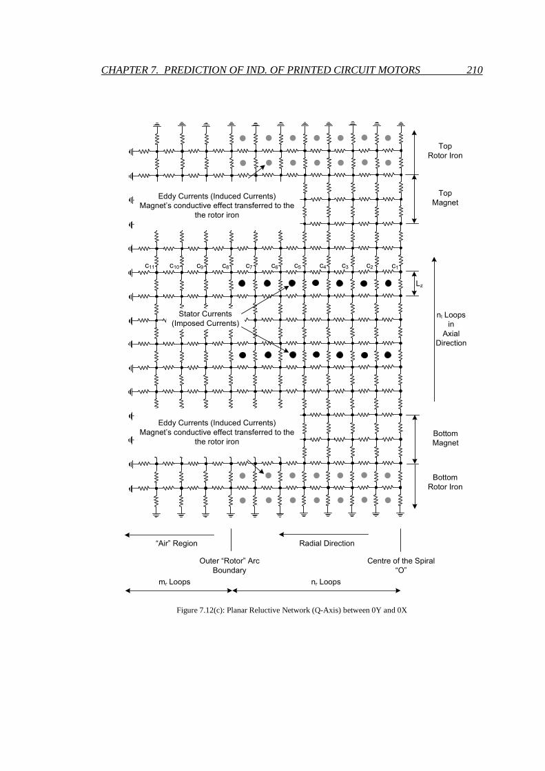
CHAPTER 7. PREDICTION OF IND. OF PRINTED CIRCUIT MOTORS 210
Figure 7.12(c): Planar Reluctive Network (Q-Axis) between 0Y and 0X
c1c2c3c4c5c6c7
Lz
nl Loops
in
Axial
Direction
Radial Direction
Top
Magnet
Top
Rotor Iron
Bottom
Magnet
Bottom
Rotor Iron
Centre of the Spiral
“O”
Outer “Rotor” Arc
Boundary
c10c11 c8c9
“Air” Region
Stator Currents
(Imposed Currents)
mr Loops nr Loops
Eddy Currents (Induced Currents)
Magnet’s conductive effect transferred to the
the rotor iron
Eddy Currents (Induced Currents)
Magnet’s conductive effect transferred to the
the rotor iron

CHAPTER 7. PREDICTION OF IND. OF PRINTED CIRCUIT MOTORS 211
This was done by distributing the conductance of the current path through the magnet equally to
the assumed rotor eddy current paths. Clearly, this constitutes an approximation. But the error
due to this approximation is not greater than about 1.5%.
7.5 Calculation of Mutual Inductances
The procedure to determine mutual inductance consists of two steps. Assuming the mutual
inductance between phase ‘a’ and phase ‘b’ is to determined, flux density distribution due to a
current of 1 A flowing through the ‘a’ phase winding is first determined. The next step consists
of evaluating the flux linking the ‘b’ phase winding.
Figure 7.13 : Determination of Mutual Inductance

CHAPTER 7. PREDICTION OF IND. OF PRINTED CIRCUIT MOTORS 212
Refer to figure 7.13. The dotted lines, radial and circumferential, define cells. A value of axial
flux density is assigned to each cell. This value is calculated by using the loop flux results from
sections 7.3 or 7.4. Flux for each axial branch is obtained in the normal manner. For example in
figure 7.9, branch flux 3mφ in figure 7.9 is equal to ( )1 3φ φ− .
Corresponding branch fluxes, one from each of the three networks (figure 7.5 or figure 7.12) are
summed to obtain the total flux for the area between neighbouring closed conducting loops.
These areas have been termed ‘sectors’ in figure 7.14. Axial flux density for each cell is defined
according to the following rules:
If, as shown in figure 7.14, the cell is not ‘cut’ by a sector boundary:
Axial flux density through cell = Sector Sector
Sector Sector
Flux
Area A
φ= (7.10)
If, as shown in figure 7.14, the cell is ‘cut’ by a sector boundary:
Axial flux density through cell =
2 32 3
2 3
Sector SectorCellFractionSector CellFractionSector
Sector Sector
Cell
A AA A
A
φ φ +
(7.11)

CHAPTER 7. PREDICTION OF IND. OF PRINTED CIRCUIT MOTORS 213
Figure 7.14 : Flux Density Distribution
Once cell flux density due to current in the ‘a’ phase winding has been determined, mutual
inductance can be computed. This is done by first calculating the flux linking each turn of the
phase winding. Summation of the flux linkage for all turns making up the ‘b’ phase winding
gives the mutual inductance between phase ‘a’ and phase ‘b’. The flux linkage for a turn is the
total axial flux enclosed by that turn. The total axial flux is computed using the flux density
values of each cell that fall within the turn. A cell that is ‘cut’ by the turn contributes an amount
of flux that is proportional to its area that falls within the turn.
Fraction of the cell area inside sector 2
Sector 2
Turn 1 (closed loop)
Turn 2 (closed loop)
Sector 3
Fraction of the cell area inside sector 3
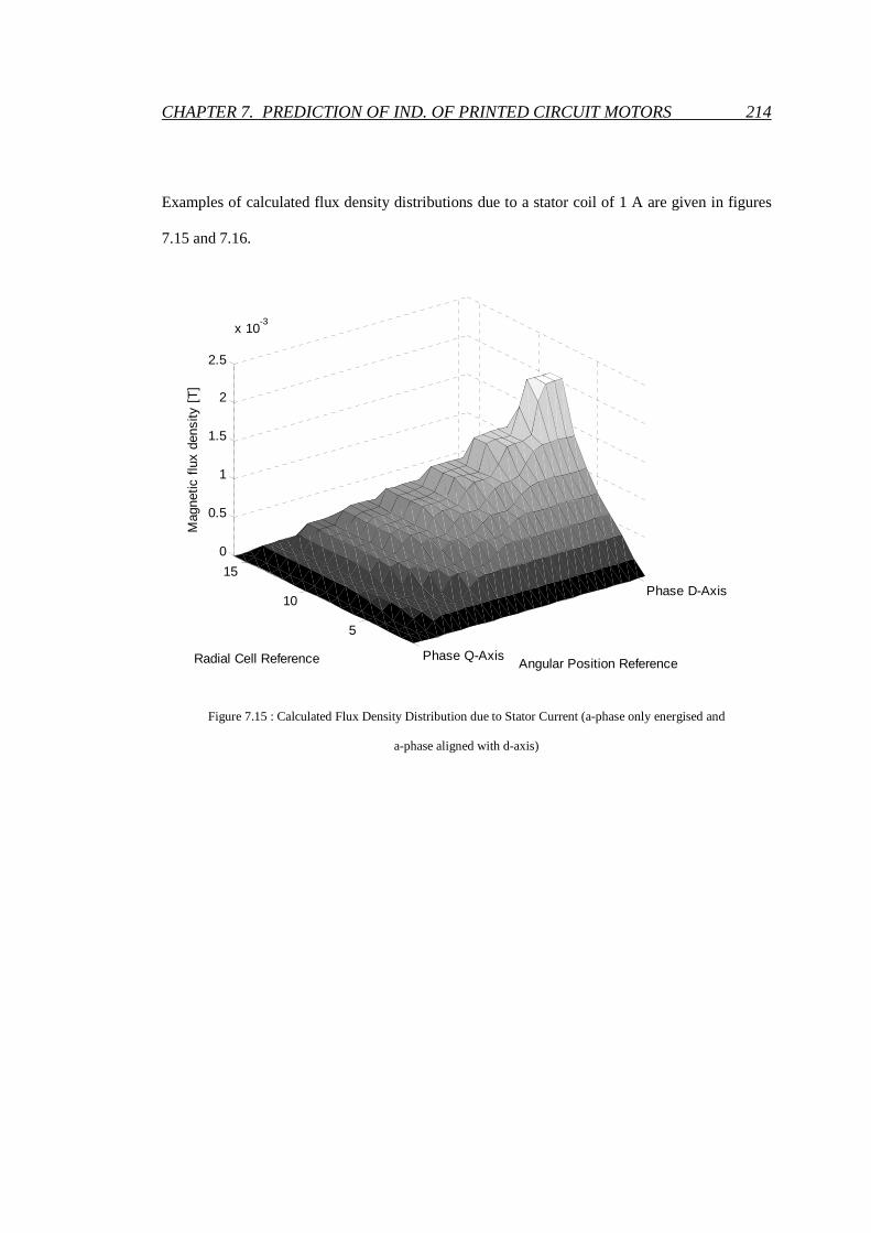
CHAPTER 7. PREDICTION OF IND. OF PRINTED CIRCUIT MOTORS 214
Examples of calculated flux density distributions due to a stator coil of 1 A are given in figures
7.15 and 7.16.
Figure 7.15 : Calculated Flux Density Distribution due to Stator Current (a-phase only energised and
a-phase aligned with d-axis)
Phase Q-Axis
Phase D-Axis
5
10
15
0
0.5
1
1.5
2
2.5
x 10-3
Angular Position ReferenceRadial Cell Reference
Mag
netic
flu
x de
nsity
[T
]

CHAPTER 7. PREDICTION OF IND. OF PRINTED CIRCUIT MOTORS 215
Figure 7.16 : Calculated Flux Density Distribution due to Stator Current (a-phase only energised and
a-phase aligned with q-axis)
Phase Q-Axis
Phase D-Axis
5
10
15
0
0.5
1
1.5
2
2.5
x 10-3
Angular Position ReferenceRadial Cell Reference
Mag
netic
flu
x de
nsity
[T
]

CHAPTER 7. PREDICTION OF IND. OF PRINTED CIRCUIT MOTORS 216
7.6 Experimental Validation
As stated in chapter 5, the assumption is that self and mutual inductances satisfy the following
equation:
( )0 2 cos 2aa s sL L L θ= + (7.12)
( ) ( )0 0 2 2
2cos 2
3bb s s s sL L L L Lπθ = + ∆ + − ∆ +
(7.13)
0 2
2cos 2
3cc s sL L Lπθ = + −
(7.14)
0 2
2cos 2
3ab ba m mL L L Lπθ = = − + −
(7.15)
( )0 2 cos 2bc cb m mL L L L θ= = − + (7.16)
( ) ( )0 0 2 2
2cos 2
3ca ac m m m mL L L L L Lπθ = = − − ∆ + − ∆ +
(7.17)
It can be deduced, based on the above assumption, that four self-inductance and four mutual
inductance values are needed to fully describe the stator’s inductance behaviour as rotor position
changes. The chosen four self-inductances are Lda, Ldb, Lqa and Lqb which are respectively the
direct and quadrature axis self-inductances of phase ‘a’ and ‘b’. The chosen mutual inductances
Mbd, Mcd, Mbq and Mcq which are respectively mutual inductances when phase ‘a’ is aligned with
the rotor direct axis and quadrature axis. Table 7.1 and 7.2 give measured and predicted values
for Lda, Ldb, Lqa, Lqb, Mbd, Mcd, Mbq and Mcq. The measured and predicted values correlate within
less than 3%.

CHAPTER 7. PREDICTION OF IND. OF PRINTED CIRCUIT MOTORS 217
Measurements were carried out at 20 kHz which is the switching frequency of the PWM voltage
applied to the test motor during normal operation. A commercial instrument was used to
measure self inductances. Based on the rated accuracy of the instrument the estimated maximum
error in the measured self-inductance is ± 0.05 µH.
The mutual inductances were measured were determined by energising one phase with a known
(measured) current and measuring the voltages induced in the other windings. The estimated
maximum error due to instrument inaccuracies is ± 0.1 µH.
Table 7.1: Measured and Predicted Self Inductances
Magnet Pitch [°]
70 60
Lda [µH] Measured 6.58 6.89
Predicted 6.64 6.99
Ldb [µH] Measured 6.78 7.09
Predicted 6.82 7.17
Lqa [µH] Measured 8.06 8.19
Predicted 7.99 8.08
Lqb [µH] Measured 7.97 8.13
Predicted 7.92 8.04

CHAPTER 7. PREDICTION OF IND. OF PRINTED CIRCUIT MOTORS 218
Table 7.2: Measured and Predicted Mutual Inductances
Magnet Pitch 70 [°]
Mbd [µH] Measured -1.52
Predicted -1.56
Mcd [µH] Measured -2.26
Predicted -2.30
Mbq [µH] Measured -2.75
Predicted -2.72
Mcq [µH] Measured -3.68
Predicted -3.64
Machine constants k1, k2, k3, k4 and k5 which were defined in chapter 5, need to be pre-loaded
into memory of the BLDC motor controller. As per equations (5.22) to (5.26), constants are
expressed in terms of Ls0, Ls2, Lm0, Lm2, ∆Ls0, ∆Ls2, ∆Lm0 and ∆Lm2 which are deduced by using:
( )0 2
da qa
s
L LL
+= (7.18)
( )2 2
qa da
s
L LL
−= (7.19)
( ) ( )0 2 2
db qb da qa
s
L L L LL
+ +∆ = − (7.20)
( ) ( )2 2 2
qa da qb db
s
L L L LL
− −∆ = − (7.21)

CHAPTER 7. PREDICTION OF IND. OF PRINTED CIRCUIT MOTORS 219
( )0 2
bd bq
m
M ML
+= − (7.22)
( )2 2
bq bd
m
M ML
−= − (7.23)
( ) ( )0 2 2
cd cq bd bq
m
M M M ML
+ +∆ = − (7.24)
( ) ( )2 2 2
cq cd bq bd
m
M M M ML
− −∆ = − (7.25)
Table 7.3 presents a comparison between values of machine constants k1 to k5 based on
theoretical prediction and those based on measurements.

CHAPTER 7. PREDICTION OF IND. OF PRINTED CIRCUIT MOTORS 220
Table 7.3: Comparison between Values of k1 to k5
k1
Measured 0.1978
Predicted 0.1846
k2 Measured 0.1813
Predicted 0.1692
k3
Measured 0.0162
Predicted 0.0148
k4 Measured 0.0836
Predicted 0.0832
k5
Measured 0.2856
Predicted 0.3035
There is reasonable agreement between measured and predicted values. It should be noted that
expected values of k3 and k4 are relatively small. This means that the percentage discrepancy
between predictions and measured values could be large. The error values in table 7.3 are useful
in that they provide designers with some idea of the expected range within which the actual
values of k1 to k5 are likely to be. Sensitivity analysis can be carried out to ensure that operation
in the sensorless mode will be satisfactory over the expected range of k1 to k5.

CHAPTER 7. PREDICTION OF IND. OF PRINTED CIRCUIT MOTORS 221
7.7 Concluding Remarks
As expected, this chapter is based on well-known equations that define the inductances of
electrical machines. However the techniques that have been developed to evaluate those
inductances are new. The techniques are based on representation of the machine by a coupled
network model. The main advantages of the proposed network are computational efficiency and
its flexibility. Difficulties arise with traditional finite element methods because of geometric
complexities and large aspect ratios of components such as air-gaps and tracks. With the
proposed method computation mesh resolution did not have to be greater than 0.04 mm and
computation times were less than 75 seconds.

222
Chapter 8
Conclusions
8
8.1 Thesis Project Achievements
The aim of this thesis project was to develop low cost systematic methods that will allow design
optimisation of sensorless axial field printed circuit brushless DC motors. In achieving this aim a
number of design tools have been developed and experimentally validated. Also a new
sensorless technique, based on inductive saliency, has been developed and tested. A summary of
the innovative features of the design tools and the sensorless technique are given below.
(d) Design equations have been derived based on geometric analyses which allow the
number of turns per printed stator coil to be maximised for commonly used coil shapes.
The coil shapes considered were the rhomboidal coil, the parallel coil and the radial coil.

CHAPTER 8. CONCLUSIONS 223
A mixed track shape, partly radial and partly parallel was developed and was found to be
the most effective shape from the point of view of torque production. The design
equations require stator inner radius, stator outer radius, clearance between tracks and
track width need to be specified. The raw calculated value for maximum number of
turns is generally a non-integer which needs to be rounded down to the nearest integer.
This provides an opportunity to increase the track width to a value higher than the
original specification.
(e) The design equations mentioned in (a) above were used to develop an algorithm and a
computer program which automatically plots the spiral shaped stator coil tracks. The
electronic version of the track plots can and have been used as input to the PCB
manufacturing process.
(f) The track plots were also used as input to another computer program which predicts
instantaneous winding EMFs and compares torque capability of alternative coil stator
designs. The program imports flux density distribution data from a 3-D non-linear
magnetostatic finite element (FEM) model of the motor. FEMLAB® was used for the
FEM model. The non-linearity results from the magnetic behaviour of the rotor being
represented by its measured magnetic saturation curve. The program uses the flux
density information to evaluate instantaneous phase EMFs at a given rotational speed.
Using the track plot it also evaluates the per phase resistance. For a given maximum
allowable resistive power loss, the torque capability of a motor is proportional to its
phase back EMF and inversely proportional to the square root of the phase resistance.

CHAPTER 8. CONCLUSIONS 224
The program can therefore be used for objective comparison of motor designs using
different track shapes. It was deduced, by using the program that the mixed track shape
results in highest torque capability for given stator dimensions. The program can also be
used to select rotor, magnet and stator axial dimensions that would result in the highest
torque rating for a given motor space envelope.
(g) The track width determined by the program described in (c) above needs to be
constrained to avoid excessive eddy current losses induced in the stator copper. A
numerical model for prediction of stator eddy current distribution has been developed.
The model, which has been validated by test results, is based on the assumption that the
eddy currents are resistively limited. In other words the inductive effects of the eddy
currents are neglected. This greatly simplifies the algorithm for determination of the
eddy current distribution. The computer program that determines the stator eddy current
loss distribution imports flux density distribution data from the 3-D non-linear
magnetostatic finite element (FEM) model described in (c) above. The copper tracks are
represented by two dimensional resistive grids. The voltage induced in each loop of the
grids at a given rotor speed is determined by using Faraday’s Law. The currents in each
branch of the grid are then determined by using loop analysis. Once the branch currents
are known, eddy current loss distribution and parasitic torque due to the eddy currents
are calculated. It was found that for the prototype machines, whose tracks were 1 mm
wide, stator eddy current loss was negligible compared to the full load stator I2R loss.
CHAPTER 8. CONCLUSIONS 225
(h) The adopted sensorless commutation technique is based on the previously reported equal
inductance method which is based on the existence of stator inductive saliency. The
advantage of the equal inductance method over the very widely used back EMF zero
crossing method is that it is effective down to zero speed. The back EMF zero crossing
method does not work below a certain level of back EMF, which means that it is useless
at low speeds. The equal inductance method is very suitable as a complement the back
EMF method. As part of this thesis project the originally proposed commutation
algorithm, based on the equal inductance method, was enhanced to achieve motor start-
up with practically zero back rotation. The enhancement consists of detection of the
motor’s initial position and energising of correct phase pair so that rotation takes place
in the desired direction.
The previously proposed equal inductance method was based on the assumption of stator
three phase symmetry. The printed circuit motors considered in this thesis project,
because of the axial position of their stators phases, exhibit significant phase asymmetry.
As a result, the equal inductance method had to be generalised to make it applicable to
those motors. Test results confirmed the effectiveness of the generalised equal
inductance method.
(i) In the case of symmetrical motors, except for a check that there is sufficient saliency, no
quantitative information on motor inductances are needed in order to implement the
equal inductance method. In the case of asymmetrical motors, stator inductance values
are needed. Those values can be obtained by measurement. However, there may be a
CHAPTER 8. CONCLUSIONS 226
need to check suitability of the equal inductance method at the design stage when
physical prototypes are not available. In that case inductance values have to be
theoretically determined. Predicted values of stator inductance are also useful for the
theoretical determination of peak stator current which can be relatively high during the
initial rotor position detection since the algorithm relies on application of bipolar PWM
with duty cycle near 50 per cent.
The rotor position estimated by the equal inductance method is proportional to the
difference between quadrature and direct axis inductances. This difference is typically of
the order of 10 to 20 percent of the average of the quadrature and direct axis
inductances. Therefore theoretical assessment of suitability of the equal inductance
method for a particular motor should be based on values of inductances that have been
determined with an accuracy of better than two or three per-cent.
An electromagnetic model, based on a hybrid of the coupled network method and the
assumed flux path method, has been developed to evaluate d-axis and q-axis phase self-
inductances and mutual inductances for printed circuit motors. Tests performed on
prototype motors gave results that were within three per-cent of values predicted from
the model. Predictions of the proposed model can be used to pre-determine the machine
constants necessary for practical implementation of sensorless commutation control
based on the equal inductance method.

CHAPTER 8. CONCLUSIONS 227
8.2 Future Work
This thesis project has focussed on the electromagnetic design and performance analysis of the
printed circuit axial flux brushless DC motor. There is a need for further investigations into the
mechanical and thermal aspects of the motor.
Accelerated aging tests need to be carried out to ensure that the stators of motors used in
practical environments remain in good condition over the design life of the motor. In particular
there is a need to find out whether mechanical and thermal stress lead to early failure resulting
from buckling of the FR4 substrate.
Only stator power losses have been investigated in this thesis project. Rotor power losses are
likely to be low, but this needs confirmation. Electromagnetic analysis is required to determine
permanent magnet and rotor iron eddy current loss. This could be based on models similar to the
ones described in (f) above. Some measure of rotor bearing and aerodynamic loss may also be of
interest to those interested in prediction of overall motor efficiency.
Prediction of thermal performance of the motor requires knowledge of heat transfer coefficients.
These are functions of rotor design, outer case design, rotor speed and the operating
environment. Modelling of air-flow inside the motor needs to be carried out to help determine
the necessary heat transfer coefficients.

CHAPTER 8. CONCLUSIONS 228
The equal inductance method requires sensing of the voltage at the terminal of the un-energised
phase of the BLDC motor. The resolution achieved by the method would theoretically allow
sensorless control of brushless motors operating in synchronous mode.
However, further research work is necessary to adapt the equal inductance method to this class
of motors because they have all three phases energised simultaneously .
It was found that the prototype motors had back emfs that were very close to sinusoidal (less
than 2% distortion). This implies that the motors are suitable for operation in synchronous mode.
If the inverter injects sinusoidal currents into phase windings, torque ripple will be minimal. The
fact that the back emf waveforms are closer to sinusoidal than trapezoidal means that torque
ripple will be present during operation of the motor in brushless DC mode. It is expected that the
motors will operate satisfactorily in the BLDC mode for most applications. Detailed
investigation aiming at minimising torque ripple in brushless DC mode remains to be done.
229
References
[1] Miller T.J.E., ‘Brushless Permanent-Magnet and Reluctance Motor Drives’, Oxford
University Press, Oxford, 1989
[2] Ahfock A. and Gambetta D., ‘Technique for Sensorless Commutation of Brushless DC
Motors ’, Swiss Institute of Intellectual Property, Bern, Patent Application Number
00342/05, 2005.
[3] Gambetta D., ‘Sensorless Technique for BLDC Motors’, MPhil Dissertation, University
of Southern Queensland, Australia, 2006
[4] Baudot J.H., ‘Rotating Electric Machines with Printed Circuit Windings’, United States
Patent Office, patent number 3144574, Aug 11, 1964.
[5] Swiggett R.L., ‘Printed Circuit Armature’, United States Patent Office, patent number
2970238, patented Jan 31, 1961.

REFERENCES 230
[6] Jang G.H. and Chang J.H., ’Development of Dual Air Gap Printed Coil BLDC Motor’,
IEEE Transaction On Magnetics, Vol. 35, No. 3, May 1999, pp. 1789-1792
[7] Tsai M. and Hsu L., ‘Design of a Miniature Axial-Flux Spindle Motor with Rhomboidal
PCB Winding’, IEEE Transactions On Magnetics, Vol 42, No. 10, October 2006, pp.
3488-3490.
[8] Jang G.H. and Chang J.H., ‘Development of an Axial-Gap Spindle Motor for Computer
Hard Disk Drives Using PCB Winding and Dual Air Gaps’, IEEE Transactions On
Magnetics, vol 38, No. 5, September 2002, pp. 3297-3299.
[9] Low T.S., Jabbar M.A. and Tan T.S., ‘Design Aspects and Performance of Slotless PM
Motor for Hard Disk Drives’, Magnetic Technology Centre, National University of
Singapore, Singapore
[10] Takano H., Ito T., Mori K. and Sakuta A., ‘Optimum Values for Magnet and Armature
Winding Thickness for Axial Field Permanent Magnet Brushless DC Motors’,
Department of Electrical Engineering, University of Osaka Prefecture, Sakai, Osaka
591, Japan
[11] Walker A.M and Pullen K.R., ‘An axial flux machine design with an airgap winding
using flat conductors’, 3rd IET International Conference on Power Electronics, Machines
and Drives (PEMD 2006), Dublin, Ireland, 4-6 April 2006, pp 221-225
REFERENCES 231
[12] Wang R and Kamper M. J., ‘Evaluation of Eddy Current Losses in Axial Flux
Permanent Magnet (AFPM) Machine with an Ironless Stator, Proceedings of IAS
Annual Meeting, 37th IEEE Industry Applications Conference IAS ’02, pp. 1289 1294
[13] Prokop L., ‘3-phase BLDC motor control with sensorless back-EMF ADC zero crossing
detection using the 56F805, Designer reference manual’ , Motorola Czech System
Laboratories, Roznov pod Radhostem, Czech Republic, 2003
[14] Bolognani S., Oboe R. and Zigliotto M., ‘Sensorless full-digital PMSM drive with EKF
estimation of speed and rotor position’, IEEE Transaction On Industrial Electronics,
Volume 46, Issue 1, 1999, pp. 184-191
[15] Kim S. and Sul S, ‘New approach for high-performance PMSM drives without
rotational position sensors’, IEEE Transaction On Power Electronics,Volume 12, Issue
5, 1997, pp. 904-911
[16] Petrovic V., Stankovic A. and Blasko V., ‘Position estimation in salient PM
synchronous motors based on PWM excitation transients’, IEEE Transaction On
Industry Applications, Volume 39, Issue 3, 2003, pp. 835-843
[17] Robeischl E. and Schroedl M., ‘Optimized INFORM measurement sequence for
sensorless PM synchronous motor drives with respect to minimum current distortion’,
IEEE Transaction On Industry Applications, Volume 40, Issue 2, 2004, pp. 591-598
REFERENCES 232
[18] Schmidt P., Gasperi M., Ray, G. and Wijenayake A., ‘Initial rotor angle detection of a
non-salient pole permanent magnet synchronous machine’, IEEE Industry Applications
Society Annual Meeting, New Orleans, 1997
[19] Shouse K. and Taylor D., ‘Sensorless velocity control of permanent-magnet synchronous
motors’, IEEE Transaction Control System Technology, Volume 6, Issue 3, 1998, pp.
313-324
[20] Wang L. and Lorenz R., ‘Rotor Position Estimation for Permanent Magnet Synchronous
Motor Using Saliency-Tracking Self-Sensing Method’, Proceedings of IEEE IAS Annual
Meeting, Rome, Italy, 2000, pp. 445-450
[21] Ueki Y., ‘Detection of relative position between magnetic pole and drive coil in
brushless dc motor’, United State Patent, Patent Number 5,159,246,1992
[22] Weiss W., ‘Artificial heart with sensorless motor’, United State Patent, Patent Number
5,751,125, 1998
[23] Lawrenson P.J. and Agu I.A., ‘Theory and performance of polyphase reluctance
machine’, ibid, 111, (8) , 1964, pp. 1435-1445
[24] ‘IEEE test procedures for synchronous machines’, IEEE publication 115, 1965, p. 52

REFERENCES 233
[25] Jones C.V., ‘The unified theory of electrical machines’, Butterworths, 1967
[26] Prescott J.C. and El-Kharashi A.K., ’A method of measuring self inductance applicable
to large electrical machines’, Proc. IEE, 106A, 1959, pp. 169-173
[27] Kaminosono H. and Uyeda K., ’New measurement of synchronous machine quantities’,
IEEE Trans., PAS-87, 1968, pp. 1908-1918
[28] Carter G.W., Leach W.I. and Sudworth J., ‘The inductance coefficients of a salient pole
alternator in relation to two-axis theory’, Proc. IEE, 108A, 1961, pp. 263-269
[29] Ahfock A. and Hart B., ‘New method for measuring Xd and Xq based on the P-Q
diagram of the lossy salient-pole machine’, IEEE Proceedings, Vol. 131, Pt. B, No. 6,
November 1984
[30] Salon S., ‘Finite Element analysis of Electrical Machines, Kluwer Academic
Publishers’, 101 Philip Drive, Assinippi Park, Norwell, Massachusetts 02061, 1995
[31] Abdel-Razek A., Coulomb J., Feliachi, M. and Sabbonnadierre, J., ‘Conception of an
air-gap element for the dynamic analysis of the electromagnetical field in electric
machines’, IEEE Transactions On Magnetics MAG-18(2) , 1982, pp. 655-659

REFERENCES 234
[32] DeBortoli M., Lee M., Salon S. and Lee K., ‘Coupling finite elements and analytical
solution in the airgap of electric machines’, IEEE Transactions On Magnetics 27(5) ,
1991, pp. 3955-3957
[33] Hewitt A. J. and Ahfock A., ‘Sub-domain scaling for finite element analysis of electrical
machines’, IEE Proceedings – Electrical Power Applications 152(2) , 2005, pp. 149-156
[34] Feliachi M., Coulomb J. and Mansir H., ‘Second order air-gap element for the dynamic
finite-element analysis of the electromagnetic field in electric machines’, IEEE
Transactions On Magnetics MAG-19(6) , 1983, pp. 2300-2303
[35] Guerin C., Tanneau G., Meunier G., Brunotte X. and Albertini J., ‘Three dimensional
magnetostatic finite elements for gaps and iron shells using magnetic scalar
potentionals’, IEEE Transactions On Magnetics 30(5) , 1994, pp. 2885-2888
[36] Bödrich, Th. Roschke, A, ‘Magnetic Library for Modelica’, Proceedings of the 4th
International Modelica Conference, Hamburg, March 7-8, 2005, Gerhard Schmitz
(editor)
[37] Petrinchenko D., Hecquet M, Brochet P., Kuznetsov V. and Laloy D., ‚Design and
Simulation of Turbo-Alternators Using a Coupled Permeance Network Model‘, IEEE
Transactions On Magnetics, Vol. 42, No. 4, 2006, pp. 1259-1262
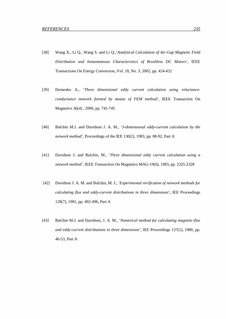
REFERENCES 235
[38] Wang X., Li Q., Wang S. and Li Q:,‘Analytical Calculation of Air-Gap Magnetic Field
Distribution and Instantaneous Characteristics of Brushless DC Motors‘, IEEE
Transactions On Energy Conversion, Vol. 18, No. 3, 2002, pp. 424-432
[39] Demenko A., ‘Three dimensional eddy current calculation using reluctance-
conductance network formed by means of FEM method’, IEEE Transaction On
Magnetics 36(4) , 2000, pp. 741-745
[40] Balchin M.J. and Davidson J. A. M., ‘3-dimensional eddy-current calculation by the
network method’, Proceedings of the IEE 130(2), 1983, pp. 88-92, Part A
[41] Davidson J. and Balchin, M., ‘Three dimensional eddy current calculation using a
network method’, IEEE Transaction On Magnetics MAG-19(6), 1983, pp. 2325-2328
[42] Davidson J. A. M. and Balchin, M. J., ‘Experimental verification of network methods for
calculating flux and eddy-current distributions in three dimensions’, IEE Proceedings
128(7), 1981, pp. 492-496, Part A
[43] Balchin M.J. and Davidson, J. A. M., ‘Numerical method for calculating magnetic-flux
and eddy-current distributions in three dimensions’, IEE Proceedings 127(1), 1980, pp.
46-53, Part A
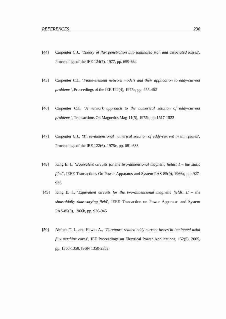
REFERENCES 236
[44] Carpenter C.J., ‘Theory of flux penetration into laminated iron and associated losses’,
Proceedings of the IEE 124(7), 1977, pp. 659-664
[45] Carpenter C.J., ‘Finite-element network models and their application to eddy-current
problems’, Proceedings of the IEE 122(4), 1975a, pp. 455-462
[46] Carpenter C.J., ‘A network approach to the numerical solution of eddy-current
problems’, Transactions On Magnetics Mag-11(5), 1975b, pp.1517-1522
[47] Carpenter C.J., ‘Three-dimensional numerical solution of eddy-current in thin plates’,
Proceedings of the IEE 122(6), 1975c, pp. 681-688
[48] King E. I., ‘Equivalent circuits for the two-dimensional magnetic fields: I – the static
filed’, IEEE Transactions On Power Apparatus and System PAS-85(9), 1966a, pp. 927-
935
[49] King E. I., ‘Equivalent circuits for the two-dimensional magnetic fields: II – the
sinusoidally time-varying field’, IEEE Transaction on Power Apparatus and System
PAS-85(9), 1966b, pp. 936-945
[50] Ahfock T. L. and Hewitt A., ‘Curvature-related eddy-current losses in laminated axial
flux machine cores’, IEE Proceedings on Electrical Power Applications, 152(5), 2005,
pp. 1350-1358. ISSN 1350-2352

REFERENCES 237
[51] Hewitt, A., ‘The effects of curvature on axial flux machine cores’, PhD Dissertation,
2005, University of Southern Queensland, Australia
[52] Guo, Y. and Zhu, J., ‘Magnetic field calculation of claw pole permanent magent
machines using magnetic network method’, Journal of Electrical and Electronics
Engineering 22(1), 2002, pp. 69-75
[53] Stöcker H., ‘Taschenbuch der Physik’, Harri Deutsch, 1998
[54] Gieras J.; Wang R-J.; Kamper M., ‘Axial Flux Permanent Magnet Brushless Machines’,
Kluwer Academic Publishers, 2004
[55] Grover F.W., ‘Inductance Calculations – Working Formulas and Tables”, 1946, D. Van
Nostrand Co., Inc.
[56] Wheeler H. A., ‘Inductance formulas for circular and square coils’ Proc. IEEE, vol. 70,
pp. 1449-1450, 1982.
[57] Miller H. C., ‘Inductance formulas for a single layer circular coil’ Proc. IEEE, vol. 75,
Issue 2, 1982.
[58] Cheng K.W.E., Chan H.L. and Sutanto D., ‘Power Electronics and Variable Speed
Drives’, 18-19 September 2000, Conference Publication No. 475, IEE 2000

238
Appendix A
First Order Magnetic Model
A.1 The model
The airgap flux density in equation (3.11) has been computed using the model geometry
presented in figure A.1.

APPENDIX A: FIRST ORDER MAGNETIC MODEL 239
mα
Figure A.1 : Model Geometry
Figure A.2 introduces the electromagnetic model relative to the geometry presented in figure A.1

APPENDIX A: FIRST ORDER MAGNETIC MODEL 240
rφ
rφ rφ
rφ
2lφ
1lφ
1dφ
2dφ
1gφ 2gφ
Figure A.2 : Model Geometry
By neglecting the leakage flux between neighbouring permanent magnets, figure A.2 can be
simplified as shown in figure A.3:
rφ
rφ rφ
rφ
gφ
Figure A.3 : Simplified Model Geometry

APPENDIX A: FIRST ORDER MAGNETIC MODEL 241
By re-arranging and grouping the various reluctances and flux sources, the model can be further
simplified as presented in figure A.4:
rφ
gφ
Figure A.4 : Further Simplified Model Geometry
A.2 Reluctance Computation
0 _
mm
r pm m
tR
Aµ µ= (A.1)
where:
( )2 2
2o i
m m
R RA
π πα
π−
= (A.2)
2
0.72m
P
π
α
= (0.7 is the clearance factor between two magnets) (A.3)
Inserting (A.2) and (A.3) in (A.1):
( )2 20 _1.4
mm
r pm o i
t PR
R Rµ µ π π=
− (A.4)

APPENDIX A: FIRST ORDER MAGNETIC MODEL 242
0g
g
gR
Aµ= (A.5)
where:
g mA A= (A.6)
Inserting (A.6) in (A.5):
( )2 201.4
g
o i
gPR
R Rµ π π=
− (A.7)
0 _
diskdisk
r disk disk
lR
Aµ µ= (A.8)
where:
( )2
22
2
o i
rdisk
R R
tl
P
π+
= +
(A.9)
( )disk o i rA R R t= − (A.10)
( )
( )0 _
22
22
o i
r
diskr disk o i r
R R
t
PR
R R t
π
µ µ
+
+ =
− (A.11)

APPENDIX A: FIRST ORDER MAGNETIC MODEL 243
A.3 Flux Density Computation
Based on figure A.4:
( )4
4 2 2m
g r
m disk g
R
R R Rφ φ=
+ + (A.12)
where:
r r mB Aφ = (Br from permanent magnet datasheet) (A.13)
( )4 1
4 2 2g m
g rg gm disk g
RB
A AR R R
φφ
= = + +
(A.14)
Assuming _r disku = ∞ and _ 1r pmu = :
2
r mg
m
B tB
gt
= +
(A.15)

244
Appendix B
First Order Stator Eddy Current
Model
B.1 The model
At first the total volume of copper winding in each track width case has been computed. Results
are presented in table B.1.

APPENDIX B: FIRST ORDER STATOR EDDY CURRENTS MODEL 245
Table B.1: Total Volume of Copper Windings (per layer)
Track
Width
[mm]
Base Cu
Thickness
[µm]
Radial+Parallel
Parts Length
[m]
Total Spiral
Length
[m]
Radial+Parallel
Parts Volume
[mm3]
Total Spiral
Volume
[mm3]
1.0 35 0.1124 0.3088 3.93 10.81
2.4 35 0.0565 0.1461 4.75 12.27
3.7 35 0.0385 0.0943 4.99 12.21
In [54] a first order model is presented, which doesn’t consider end-windings. The author knows
that at certain rotor positions eddy current are also induced in the end-winding, but for a first
estimation of the eddy current losses, this approximation is applicable and as shown, the results
are acceptable.
2 22 2 2 2 2 2
3 3e con mz con mzP f a m B f a V Bπ σ π σ
ρ∆ = = (B.1)
where:
σ = Electric conductivity = 47e6 S/m
f = Frequency (electrical) at 1000 rpm = 33.33 Hz
a = Track width = 1e-3 / 2.4e-3 / 3.7e-3 m
Vcon = Conductor volume without end-winding = 3.93e-9 / 4.75e-9 / 4.99e-9 m3

APPENDIX B: FIRST ORDER STATOR EDDY CURRENTS MODEL 246
Bmz = Peak Axial flux density = 0.7 T
The formula assumes a sinusoidal flux density distribution (no distortion)
Table B.2: Predicted Loss per Phase
Track Width
[mm]
Total Eddy Current Loss
[mW]
1.0 3.8
2.4 26.4
3.7 65.6
Agreement with results presented in chapter 6 is within 20%.

247
Appendix C
First Order Self Inductance Model
C.1 The model
Different publications are available on inductance computation of single layer and spiral coils. A
very interesting handbook on inductance calculations has been published by [55]. This book
represents a nice short cut for engineers or designers. An analytical formula for the self-
inductance of a single layer circular coil of any lenght
diameterratio has been given by Wheeler [56]:
2 2N rL K
c
µ π= (C.1)
where:

APPENDIX C: FIRST ORDER SELF INDUCTANCE MODEL 248
( ) ( ) ( )2
1 4 8
3
dc d rK F k E k E k
r c cπ = − − −
r = radius of the coil
c = axial length of the coil
d = 2 24r c−
N = number of turns
K = 2r
d
F(k), E(k) = Elliptic integrals of first and second order
A closed solution of the elliptic integrals is not immediate. Miller [57] introduced an iterative
method to determine F(k) and E(k). The primary objective of the intended first order model is a
fast estimation of the motor phase self inductance. This is useful for first evaluation of control
possibilities of the planned machines. Therefore the formula should not contain iterative loops,
which would require significant computational effort.
Chan, Cheng and Sutanto [58] introduced a simplification of the Neumann’s Formula. In this
case the elliptic integrals are approximated by a logarithmic function.
To overcome difficulties with elliptic integrals, Wheeler [56] published different approximate
formulae, which are nowadays well diffused. In one particular case he derived an approximation
for a spirally shaped coplanar coil, by collapsing the coplanar turns in one “mean” turn under
assumption that the conductor width is much larger than the clearance between each conductor.

APPENDIX C: FIRST ORDER SELF INDUCTANCE MODEL 249
This is a reasonable assumption also in the case of printed circuit spiral. The flat spiral air-core
coil inductance by Wheeler [56] can be easily computed by:
( )2 2
52 2.8 10 g
N rL k
r d=
+ (C.2)
where:
r = mean radius of the coil
c= axial length of the coil
d= outer coil radius (ro) - outer coil radius (ri)
and,
2 ps opsg
cs
l lk P
l
−= ⋅ , where:
P= number of stator poles
lcs= length of the circular spiral (used by equation (2)) 2r Nπ≅
lps= length of the phase spiral (real track shape from algorithm).
lps= length of the outer arcs of the spiral (real track shape from algorithm).
The inductance computed by (C.2) is in free space. This condition is not reflected in the motor.
By measurements presented in figure 7.10, the coil q-axis inductance is near to the coil
inductance in free space.
The first order model delivers a value which is closer to the q-axis inductance, within 25%.

250
Appendix D
Photo Gallery
D.1 Photos of Hardware
Figure D.1 : The Motor Prototype
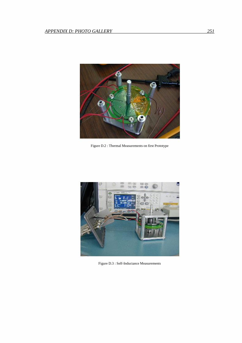
APPENDIX D: PHOTO GALLERY 251
Figure D.2 : Thermal Measurements on first Prototype
Figure D.3 : Self-Inductance Measurements