slide 1

Neural Networks

Xiaojin Zhu

jerryzhu@cs.wisc.edu

Computer Sciences Department

University of Wisconsin, Madison

slide 2

Terminator 2 (1991)

JOHN: Can you learn? So you can be... you know. More human. Not such a

dork all the time.

TERMINATOR: My CPU is a neural-net processor... a learning computer.

But Skynet presets the switch to "read-only" when we are sent out alone.

…

TERMINATOR Basically. (starting the engine, backing out) The Skynet

funding bill is passed. The system goes on-line August 4th, 1997. Human

decisions are removed from strategic defense. Skynet begins to learn, at a

geometric rate. It becomes self-aware at 2:14 a.m. eastern time, August 29.

In a panic, they try to pull the plug.

SARAH: And Skynet fights back.

TERMINATOR: Yes. It launches its ICBMs against their targets in Russia.

SARAH: Why attack Russia?

TERMINATOR: Because Skynet knows the Russian counter-strike will

remove its enemies here.

We’ll learn how to set the neural net

slide 3

Outline

• A single neuron

Linear perceptron

Non-linear perceptron

Learning of a single perceptron

The power of a single perceptron

• Neural network: a network of neurons

Layers, hidden units

Learning of neural network: backpropagation

The power of neural network

Issues

• Everything revolves around gradient descent

slide 4

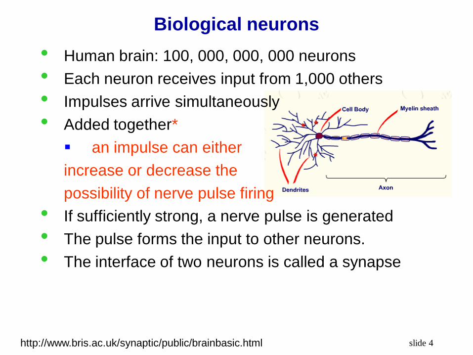
Biological neurons

• Human brain: 100, 000, 000, 000 neurons

• Each neuron receives input from 1,000 others

• Impulses arrive simultaneously

• Added together*

an impulse can either

increase or decrease the

possibility of nerve pulse firing

• If sufficiently strong, a nerve pulse is generated

• The pulse forms the input to other neurons.

• The interface of two neurons is called a synapse

http://www.bris.ac.uk/synaptic/public/brainbasic.html

slide 5

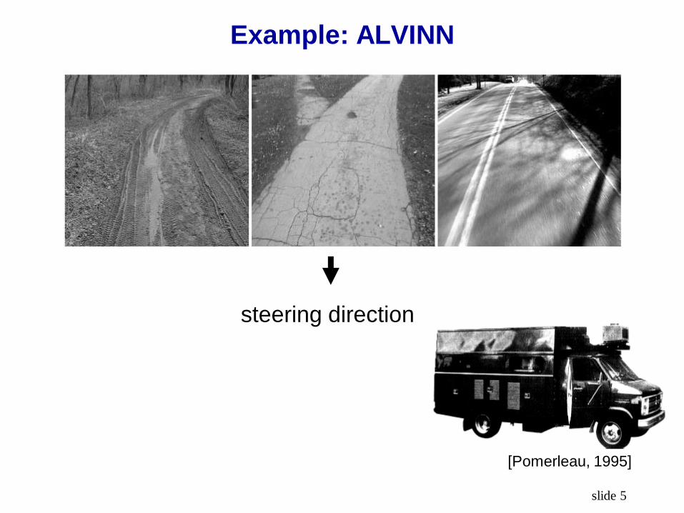
Example: ALVINN

[Pomerleau, 1995]

steering direction

slide 6

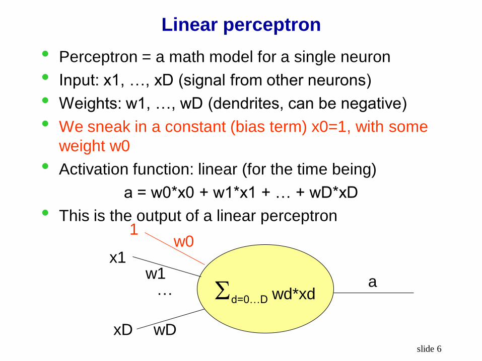
Linear perceptron

• Perceptron = a math model for a single neuron

• Input: x1, …, xD (signal from other neurons)

• Weights: w1, …, wD (dendrites, can be negative)

• We sneak in a constant (bias term) x0=1, with some

weight w0

• Activation function: linear (for the time being)

a = w0*x0 + w1*x1 + … + wD*xD

• This is the output of a linear perceptron

d=0…D wd*xd … w1

wD

w0 1

x1

xD

a

slide 7

Learning in linear perceptron

• Regression. Training data {(X1, y1), …, (XN, yN)}

• X1 is a vector: (x11, …, x1D), so are X2…XN

• y1 is a real-valued output

• Goal: learn the weights w0…wD, so that given input

Xi, the output of the perceptron ai is close to yi

• Define “close”:

E = ½ i=1..N (ai-yi)2

• E is the “error”. Given the training set, E is a function

of w0…wD.

• Minimize E: unconstrained optimization. Variables

w0…wD.

slide 8

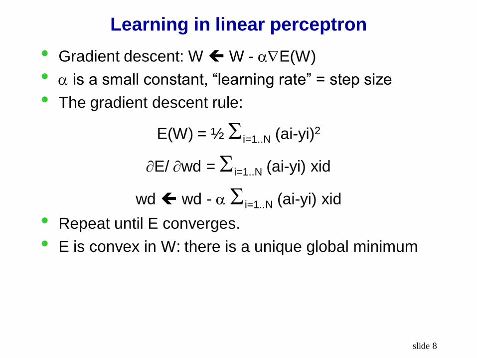
Learning in linear perceptron

• Gradient descent: W W - E(W)

• is a small constant, “learning rate” = step size

• The gradient descent rule:

E(W) = ½ i=1..N (ai-yi)2

E/ wd = i=1..N (ai-yi) xid

wd wd - i=1..N (ai-yi) xid

• Repeat until E converges.

• E is convex in W: there is a unique global minimum

slide 9

The (limited) power of linear perceptron

• Linear perceptron is just

a=W’X

• where X is the input vector, augmented by x0=1

• It can represent any linear function in D+1

dimensional space… but that’s it

• In particular, it won’t be a nice fit to binary

classification (y=0 or y=1)

1

slide 10

Non-linear perceptron

• Change the activation function: use a step function

a = g(w0*x0 + w1*x1 + … + wD*xD)

• g(h)=0, if h < 0; g(h)=1 if h0

• Can you see how to make logic AND, OR, NOT with

such a perceptron?

g(d=0…D wd*xd) … w1

wD

w0 1

x1

xD

a

slide 11

Linear Threshold Unit (LTU):

Our first non-linear perceptron • Change the activation function: use a step function

a = g(w0*x0 + w1*x1 + … + wD*xD)

• g(h)=0, if h < 0; g(h)=1 if h0

• AND: w1=w2=1, w0= -1.5

• OR: w1=w2=1, w0= -0.5

• NOT: w1= -1, w0= 0.5

g(d=0…D wd*xd) … w1

wD

w0 1

x1

xD

a

Now we see the reason

for bias terms

slide 12

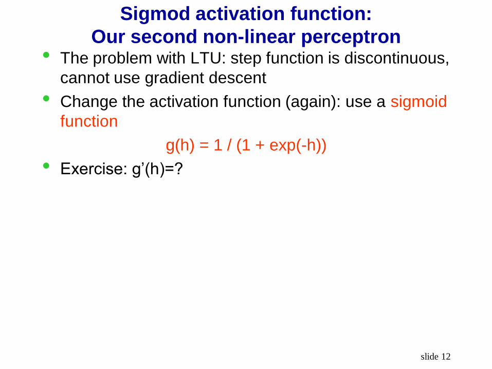
Sigmod activation function:

Our second non-linear perceptron • The problem with LTU: step function is discontinuous,

cannot use gradient descent

• Change the activation function (again): use a sigmoid

function

g(h) = 1 / (1 + exp(-h))

• Exercise: g’(h)=?

slide 13

• The problem with LTU: step function is discontinuous,

cannot use gradient descent

• Change the activation function (again): use a sigmoid

function

g(h) = 1 / (1 + exp(-h))

• Exercise: g’(h)= g(h) (1-g(h))

Sigmod activation function:

Our second non-linear perceptron

slide 14

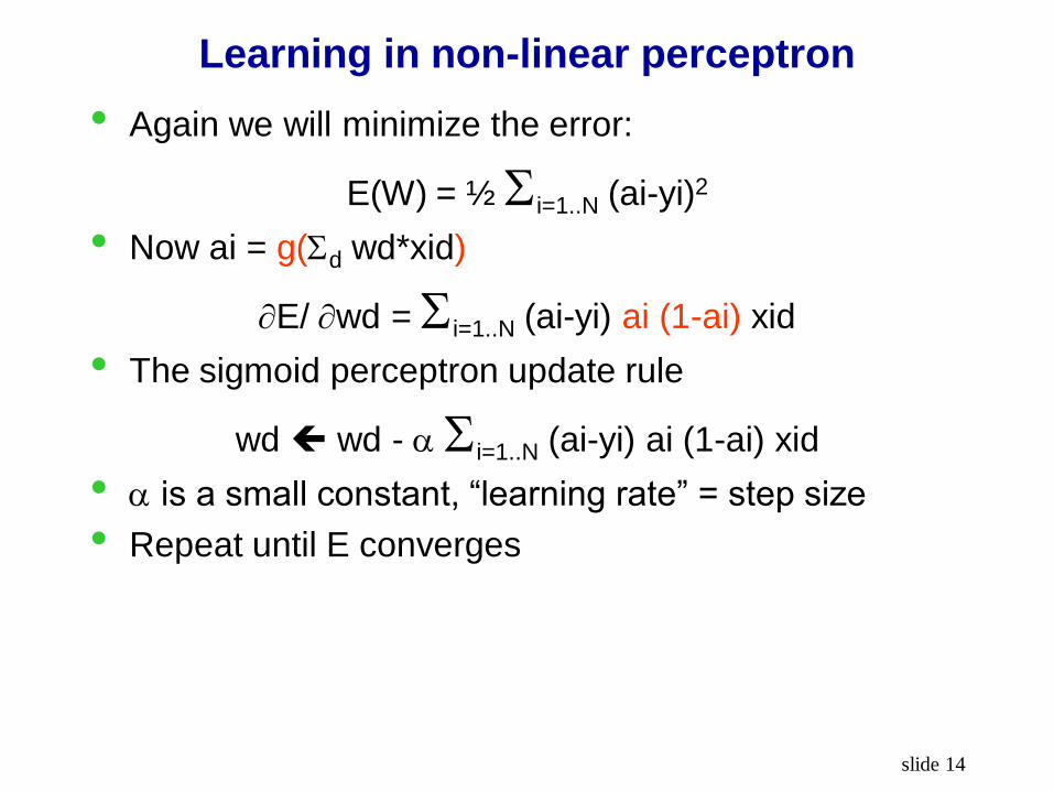
Learning in non-linear perceptron

• Again we will minimize the error:

E(W) = ½ i=1..N (ai-yi)2

• Now ai = g(d wd*xid)

E/ wd = i=1..N (ai-yi) ai (1-ai) xid

• The sigmoid perceptron update rule

wd wd - i=1..N (ai-yi) ai (1-ai) xid

• is a small constant, “learning rate” = step size

• Repeat until E converges

slide 15

The (limited) power of non-linear perceptron

• Even with a non-linear sigmoid function, the decision

boundary a perceptron can produce is still linear

• AND, OR, NOT revisited

• How about XOR?

slide 16

The (limited) power of non-linear perceptron

• Even with a non-linear sigmoid function, the decision

boundary a perceptron can produce is still linear

• AND, OR, NOT revisited

• How about XOR?

• This contributed to the first AI winter

slide 17

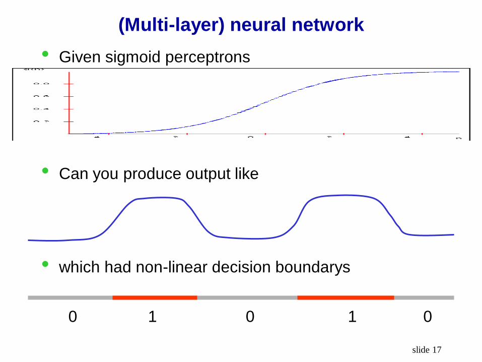
(Multi-layer) neural network

• Given sigmoid perceptrons

• Can you produce output like

• which had non-linear decision boundarys

0 1 0 1 0

slide 18

Multi-layer neural network

• There are many ways to connect perceptrons into a

network. One standard way is multi-layer neural nets

• 1 Hidden layer: we can’t see the output; 1 output

layer

HIDN

k

kkvWg1

Out

INS

INS

INS

N

k

kk

N

k

kk

N

k

kk

xwgv

xwgv

xwgv

1

33

1

22

1

11

x1

x2

w11

w21

w31

w1

w2

w3

w32

w22

w12

[from Andrew Moore]

slide 19

The (unlimited) power of neural network

• In theory

we don’t need too many layers:

1-hidden-layer net with enough hidden units can

represent any continuous function of the inputs

with arbitrary accuracy

2-hidden-layer net can even represent

discontinuous functions

slide 20

Neural net for K-way classification

• Use K output units. During training, encode a label y

by an indicator vector with K entries:

class1=(1,0,0,…,0), class2=(0,1,0,…,0) etc.

• During test (decoding), choose the class

corresponding to the largest output unit

HIDN

k

kkvWg1

Out

INS

INS

INS

N

k

kk

N

k

kk

N

k

kk

xwgv

xwgv

xwgv

1

33

1

22

1

11

x1

x2

HIDN

k

kkvWg1

Out

…

out 1

out K

slide 21

Example Y encoding

[Pomerleau, 1995]

slide 22

Obtaining training data

[Pomerleau, 1995]

slide 23

Learning in neural network

• Again we will minimize the error (K outputs):

E(W) = ½ i=1..N c=1..K (oic-Yic)2

• i: the i-th training point

• oic: the c-th output for the i-th training point

• Yic: the c-th element of the i-th label indicator vector

• Our variables are all the weights w on all the edges

Apparent difficulty: we don’t know the ‘correct’

output of hidden units

It turns out to be OK: we can still do gradient

descent. The trick you need is the chain rule

The algorithm is known as back-propagation

slide 24

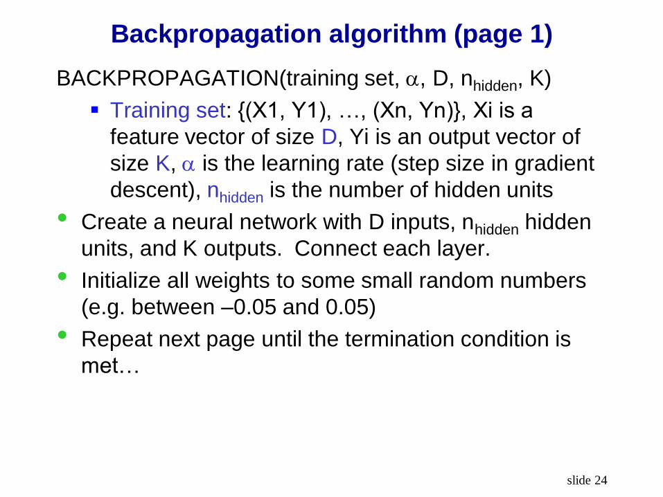
Backpropagation algorithm (page 1)

BACKPROPAGATION(training set, , D, nhidden, K)

Training set: {(X1, Y1), …, (Xn, Yn)}, Xi is a

feature vector of size D, Yi is an output vector of

size K, is the learning rate (step size in gradient

descent), nhidden is the number of hidden units

• Create a neural network with D inputs, nhidden hidden

units, and K outputs. Connect each layer.

• Initialize all weights to some small random numbers

(e.g. between –0.05 and 0.05)

• Repeat next page until the termination condition is

met…

slide 25

Backpropagation algorithm (page 2)

For each training example (X, Y):

• Propagate the input forward through the network

Input X to the network, compute output ou for every unit u in the network

• Propagate the errors backward through the network

for each output unit c, compute its error term c

for each hidden unit h, compute its error term h

update each weight wji

• where xji is the input from unit i into unit j (oi if i is a hidden unit; Xi if i is an input)

• wji is the weight from unit i to unit j

)1()( ccccc ooyo

)1()(

hh

hsucci

iihh oow

jijjiji xww

slide 26

Derivation of backpropagation

• For simplicity we assume online learning (as oppose

to batch learning): 1-step gradient descent after

seeing each training example (X,Y)

• For each (X,Y), the error is

E(W) = ½ c=1..K (oc-Yc)2

oc: the c-th output unit (when input is X)

Yc: the c-th element of the label indicator vector

• Use gradient descent to change all the weights wji to

minimize the error. Separate two cases:

Case 1: wji when j is an output unit

Case 2: wji when j is a hidden unit

slide 27

Case 1: weights of an output unit

oc: the c-th output unit (when input is X)

Yc: the c-th element of the label indicator vector

• gradient descent: to minimize error, run away from

the partial derivative

j

oj

i

yj

wji

xji jijjjj

ji

j

m

jmjm

ji

jj

ji

xooyo

w

yxwg

w

yo

w

Error

)1()(

))((2

1)(

2

1 22

jijjjjji

ji

jiji xooyoww

Errorww )1()(

slide 28

Case 2: weights of a hidden unit

j

oj

c

yc

wji

xji

oc

jijjcjcc

jsuccc

cc

ji

n

jnjn

cm

m

cmcm

jsuccc

cc

ji

j

j

c

jsuccc c

c

ji

xoowooyo

w

xwg

x

xwg

yo

w

o

o

o

o

E

w

Error

)1()1()(

)()(

)(

)(

)(

)(

slide 29

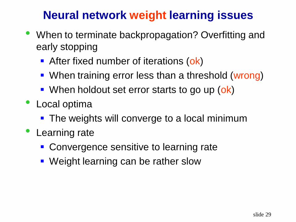
Neural network weight learning issues

• When to terminate backpropagation? Overfitting and

early stopping

After fixed number of iterations (ok)

When training error less than a threshold (wrong)

When holdout set error starts to go up (ok)

• Local optima

The weights will converge to a local minimum

• Learning rate

Convergence sensitive to learning rate

Weight learning can be rather slow

slide 30

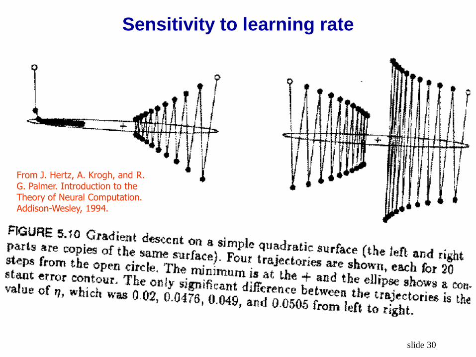
Sensitivity to learning rate

From J. Hertz, A. Krogh, and R. G. Palmer. Introduction to the Theory of Neural Computation. Addison-Wesley, 1994.

slide 31

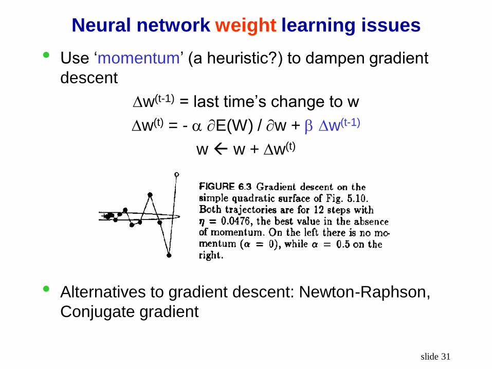
Neural network weight learning issues

• Use ‘momentum’ (a heuristic?) to dampen gradient

descent

w(t-1) = last time’s change to w

w(t) = - E(W) / w + w(t-1)

w w + w(t)

• Alternatives to gradient descent: Newton-Raphson,

Conjugate gradient

slide 32

Neural network structure learning issues

• How many hidden units?

• How many layers?

• How to connect units?

• Cross validation