Perceptrons and Neural Networkspages.cs.wisc.edu/~bgibson/cs540/handouts/neural.pdf · Outline I Perceptron: a single neuron I Linear perceptron I Non-linear perceptron I Learning

ML (cont.): Perceptrons and Neural Networks

CS540 Bryan R Gibson University of Wisconsin-Madison

Slides adapted from those used by Prof. Jerry Zhu, CS540-1

1 / 25

slide 2

Terminator 2 (1991)

JOHN: Can you learn? So you can be... you know. More human. Not such a dork all the time.

TERMINATOR: My CPU is a neural-net processor... a learning computer. But Skynet presets the switch to "read-only" when we are sent out alone.

«

TERMINATOR Basically. (starting the engine, backing out) The Skynet funding bill is passed. The system goes on-line August 4th, 1997. Human decisions are removed from strategic defense. Skynet begins to learn, at a geometric rate. It becomes self-aware at 2:14 a.m. eastern time, August 29. In a panic, they try to pull the plug.

SARAH: And Skynet fights back.

TERMINATOR: Yes. It launches its ICBMs against their targets in Russia.

SARAH: Why attack Russia?

TERMINATOR: Because Skynet knows the Russian counter-strike will remove its enemies here.

:H¶OO�OHDUQ�KRZ�WR�set the neural net

Outline

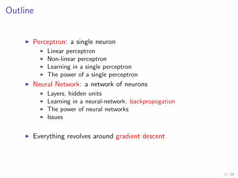
I Perceptron: a single neuronI Linear perceptronI Non-linear perceptronI Learning in a single perceptronI The power of a single perceptron

I Neural Network: a network of neuronsI Layers, hidden unitsI Learning in a neural-network: backpropogationI The power of neural networksI Issues

I Everything revolves around gradient descent

2 / 25

Biological Neurons

I Human brain: around a hundred trillion neurons

I Each neuron receives input from 1,000’s of others

I Impulses arrive simultaneouslyI Then they’re added together

I an impulse can either increase or decrease the possibility of anerve pulse firing

I If sufficiently strong, a nerve pulse is generated

I The pulse becomes and input to other neurons

3 / 25

slide 5

Example: ALVINN

[Pomerleau, 1995]

steering direction

Linear PerceptronI Perceptron: a math model for a single neuronI Input: x1, . . . , xd (signals from other neurons)I Weights: w1, . . . , wd (dendrites, can be negative!)I We sneak in a constant (bias term) x0, with weight w0

I Activation function: linear (for now)

a = w0x0 + w1x1 + . . .+ wdxd

I This a is the output of a linear perceptron

x1

x2

. . .

xd

1

∑dj=0wjxj

a

w1

w2

wd

w0

4 / 25

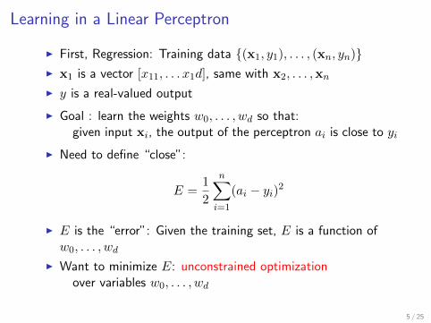
Learning in a Linear Perceptron

I First, Regression: Training data {(x1, y1), . . . , (xn, yn)}I x1 is a vector [x11, . . . x1d], same with x2, . . . ,xn

I y is a real-valued output

I Goal : learn the weights w0, . . . , wd so that:given input xi, the output of the perceptron ai is close to yi

I Need to define “close”:

E =1

2

n∑i=1

(ai − yi)2

I E is the “error”: Given the training set, E is a function ofw0, . . . , wd

I Want to minimize E: unconstrained optimizationover variables w0, . . . , wd

5 / 25

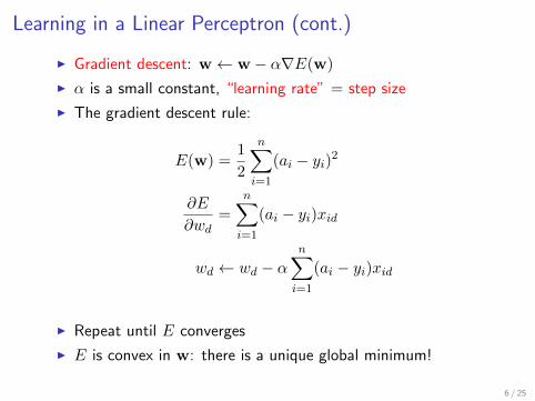
Learning in a Linear Perceptron (cont.)

I Gradient descent: w← w − α∇E(w)

I α is a small constant, “learning rate” = step size

I The gradient descent rule:

E(w) =1

2

n∑i=1

(ai − yi)2

∂E

∂wd=

n∑i=1

(ai − yi)xid

wd ← wd − αn∑

i=1

(ai − yi)xid

I Repeat until E converges

I E is convex in w: there is a unique global minimum!

6 / 25





E(w) =1

2

n∑i=1

(ai − yi)2

∂E

∂wd=

n∑i=1

(ai − yi)xid


i=1

(ai − yi)xid



6 / 25





E(w) =1

2

n∑i=1

(ai − yi)2

∂E

∂wd=

n∑i=1

(ai − yi)xid


i=1

(ai − yi)xid



6 / 25





E(w) =1

2

n∑i=1

(ai − yi)2

∂E

∂wd=

n∑i=1

(ai − yi)xid


i=1

(ai − yi)xid



6 / 25





E(w) =1

2

n∑i=1

(ai − yi)2

∂E

∂wd=

n∑i=1

(ai − yi)xid


i=1

(ai − yi)xid



6 / 25





E(w) =1

2

n∑i=1

(ai − yi)2

∂E

∂wd=

n∑i=1

(ai − yi)xid


i=1

(ai − yi)xid



6 / 25





E(w) =1

2

n∑i=1

(ai − yi)2

∂E

∂wd=

n∑i=1

(ai − yi)xid


i=1

(ai − yi)xid



6 / 25

The (Limited) Power of a Linear Perceptron

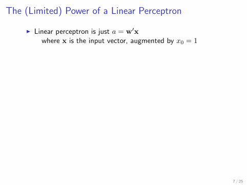
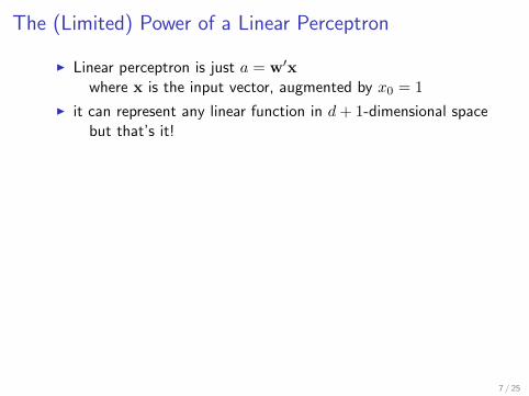
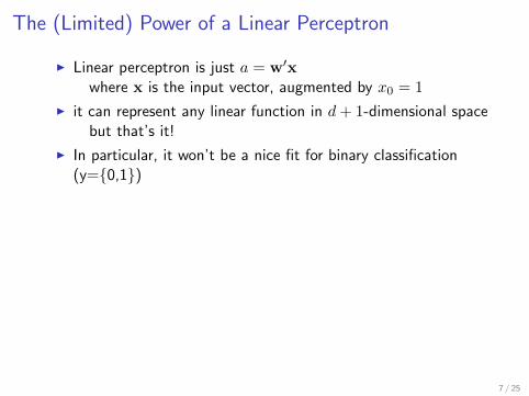
I Linear perceptron is just a = w′xwhere x is the input vector, augmented by x0 = 1

I it can represent any linear function in d+ 1-dimensional spacebut that’s it!

I In particular, it won’t be a nice fit for binary classification(y={0,1})

1

?

7 / 25





1

?

7 / 25





1

?

7 / 25





1

?

7 / 25





1

?

7 / 25





1

?

7 / 25

Non-Linear Perceptron

I Change the activation function: use a step function

a = g(w0x0 + w1x1 + . . .+ wdxd)

g(h) = 1{h ≥ 0}

I This is called a Linear Threshold Unit (LTU)

x1

x2

. . .

xd

1

g(∑d

j=0wjxj

)a

w1

w2

wd

w0

I Can you see how to make logical AND, OR, NOT functionsusing this perceptron?

8 / 25

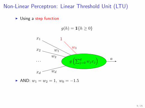
Non-Linear Perceptron: Linear Threshold Unit (LTU)

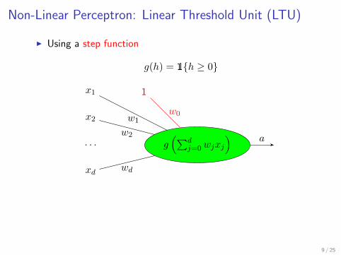
I Using a step function

g(h) = 1{h ≥ 0}

x1

x2

. . .

xd

1

g(∑d

j=0wjxj

)a

w1

w2

wd

w0

I AND: w1 = w2 = 1, w0 = −1.5

I OR: w1 = w2 = 1, w0 = −0.5

I NOT: w1 = −1, w0 = 0.5

9 / 25



g(h) = 1{h ≥ 0}

x1

x2

. . .

xd

1

g(∑d

j=0wjxj

)a

w1

w2

wd

w0

I AND: w1 = w2 = 1, w0 = −1.5

I OR: w1 = w2 = 1, w0 = −0.5

I NOT: w1 = −1, w0 = 0.5

9 / 25



g(h) = 1{h ≥ 0}

x1

x2

. . .

xd

1

g(∑d

j=0wjxj

)a

w1

w2

wd

w0

I AND: w1 = w2 = 1, w0 = −1.5

I OR: w1 = w2 = 1, w0 = −0.5

I NOT: w1 = −1, w0 = 0.5

9 / 25



g(h) = 1{h ≥ 0}

x1

x2

. . .

xd

1

g(∑d

j=0wjxj

)a

w1

w2

wd

w0

I AND: w1 = w2 = 1, w0 = −1.5

I OR: w1 = w2 = 1, w0 = −0.5

I NOT: w1 = −1, w0 = 0.5

9 / 25

Non-Linear Perceptron: Sigmoid Activation Function

I The problem with LTU: step function is discontinuous,cannot use gradient descent!

I Change the activation function (again): use a sigmoid function

g(h) =1(

1 + e(−h))

I Exercise: g′(h) = ?

I Exercise: g′(h) = g(h) (1− g(h))

−6 −4 −2 2 4 6

0.2

0.4

0.6

0.8

1

10 / 25

Non-Linear Perceptron: Sigmoid Activation Function

I The problem with LTU: step function is discontinuous,cannot use gradient descent!

I Change the activation function (again): use a sigmoid function

g(h) =1(

1 + e(−h))

I Exercise: g′(h) = g(h) (1− g(h))

−6 −4 −2 2 4 6

0.2

0.4

0.6

0.8

1

10 / 25

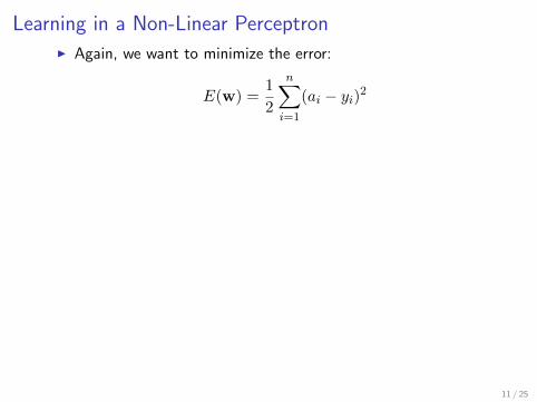
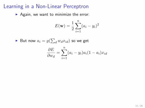
Learning in a Non-Linear PerceptronI Again, we want to minimize the error:

E(w) =1

2

n∑i=1

(ai − yi)2

I But now ai = g(∑

dwdxid) so we get

∂E

∂wd=

n∑i=1

(ai − yi)ai(1− ai)xid

I The sigmoid perceptron update rule is then


i=1


I Again, α is a small constant, the step size or learning rateI Repeat until E converges

11 / 25


E(w) =1

2

n∑i=1

(ai − yi)2


dwdxid) so we get

∂E

∂wd=

n∑i=1




i=1



11 / 25


E(w) =1

2

n∑i=1

(ai − yi)2


dwdxid) so we get

∂E

∂wd=

n∑i=1




i=1



11 / 25


E(w) =1

2

n∑i=1

(ai − yi)2


dwdxid) so we get

∂E

∂wd=

n∑i=1




i=1



11 / 25


E(w) =1

2

n∑i=1

(ai − yi)2


dwdxid) so we get

∂E

∂wd=

n∑i=1




i=1



11 / 25


E(w) =1

2

n∑i=1

(ai − yi)2


dwdxid) so we get

∂E

∂wd=

n∑i=1




i=1



11 / 25


E(w) =1

2

n∑i=1

(ai − yi)2


dwdxid) so we get

∂E

∂wd=

n∑i=1




i=1



11 / 25

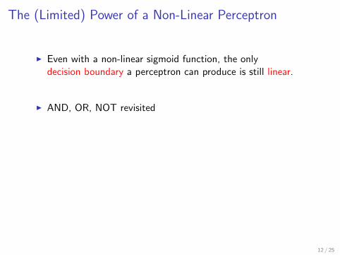
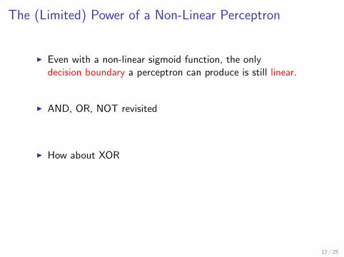
The (Limited) Power of a Non-Linear Perceptron

I Even with a non-linear sigmoid function, the onlydecision boundary a perceptron can produce is still linear.

I AND, OR, NOT revisited

I How about XOR

I This contributed to the first AI winter

12 / 25




I How about XOR


12 / 25




I How about XOR


12 / 25




I How about XOR


12 / 25

(Multi-Layer) Neural Networks

I Given sigmoid perceptrons . . .

−6 −4 −2 2 4 6

0.2

0.4

0.6

0.8

1

I can you produce output like . . .

−7 −6 −5 −4 −3 −2 −1 0 1 2 3 4 5 6 7

I which has a non-linear decision boundary?

+ - + - +

13 / 25

Mulit-Layer Neural Networks

I There are many ways to make a network of perceptrons.

I One standard way is multi-layer neural nets.

I 1 hidden layer (we can’t see the output); 1 output layer

x1

x2

v1 = g (∑nin

k=1 w1kxk)

v2 = g (∑nin

k=1 w2kxk)

v3 = g (∑nin

k=1 w3kxk)

o = g (∑nhidden

k=1 wkvk)

w11

w21

w31

w12

w22

w32

w1

w2

w3

14 / 25

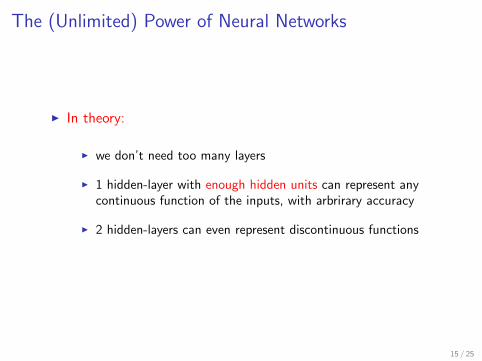
The (Unlimited) Power of Neural Networks

I In theory:

I we don’t need too many layers

I 1 hidden-layer with enough hidden units can represent anycontinuous function of the inputs, with arbrirary accuracy

I 2 hidden-layers can even represent discontinuous functions

15 / 25

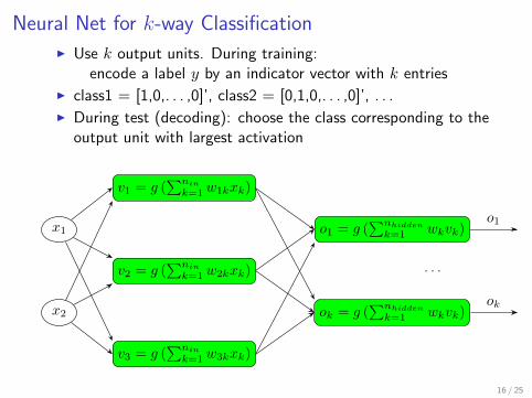
Neural Net for k-way Classification

I Use k output units. During training:encode a label y by an indicator vector with k entries

I class1 = [1,0,. . . ,0]’, class2 = [0,1,0,. . . ,0]’, . . .

I During test (decoding): choose the class corresponding to theoutput unit with largest activation

x1

x2

v1 = g (∑nin

k=1 w1kxk)

v2 = g (∑nin

k=1 w2kxk)

v3 = g (∑nin

k=1 w3kxk)

o1 = g (∑nhidden

k=1 wkvk)

. . .

ok = g (∑nhidden

k=1 wkvk)

o1

ok

16 / 25

slide 21

Example Y encoding

[Pomerleau, 1995]

slide 22

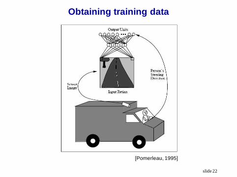
Obtaining training data

[Pomerleau, 1995]

Learning in a Neural Network

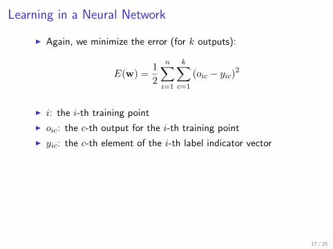
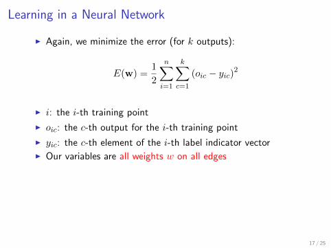
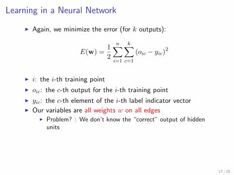
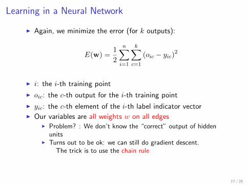
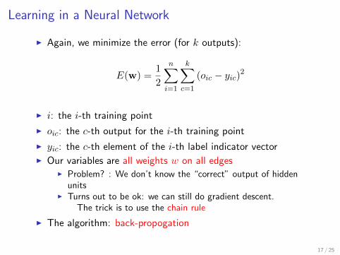
I Again, we minimize the error (for k outputs):

E(w) =1

2

n∑i=1

k∑c=1

(oic − yic)2

I i: the i-th training point

I oic: the c-th output for the i-th training point

I yic: the c-th element of the i-th label indicator vectorI Our variables are all weights w on all edges

I Problem? : We don’t know the “correct” output of hiddenunits

I Turns out to be ok: we can still do gradient descent.The trick is to use the chain rule

I The algorithm: back-propogation

17 / 25



E(w) =1

2

n∑i=1

k∑c=1

(oic − yic)2







17 / 25



E(w) =1

2

n∑i=1

k∑c=1

(oic − yic)2







17 / 25



E(w) =1

2

n∑i=1

k∑c=1

(oic − yic)2



I yic: the c-th element of the i-th label indicator vector

I Our variables are all weights w on all edgesI Problem? : We don’t know the “correct” output of hidden

unitsI Turns out to be ok: we can still do gradient descent.

The trick is to use the chain rule


17 / 25



E(w) =1

2

n∑i=1

k∑c=1

(oic − yic)2







17 / 25



E(w) =1

2

n∑i=1

k∑c=1

(oic − yic)2







17 / 25



E(w) =1

2

n∑i=1

k∑c=1

(oic − yic)2







17 / 25



E(w) =1

2

n∑i=1

k∑c=1

(oic − yic)2







17 / 25

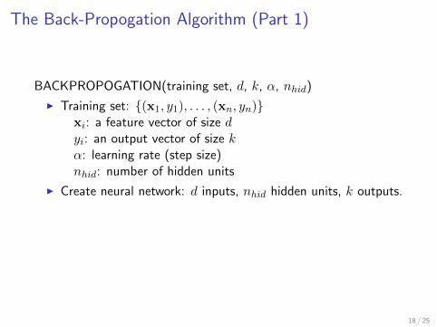
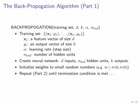
The Back-Propogation Algorithm (Part 1)

BACKPROPOGATION(training set, d, k, α, nhid)

I Training set: {(x1, y1), . . . , (xn, yn)}xi: a feature vector of size dyi: an output vector of size kα: learning rate (step size)nhid: number of hidden units

I Create neural network: d inputs, nhid hidden units, k outputs.

I Initialize weights to small random numbers (e.g. in [−0.05, 0.05])

I Repeat (Part 2) until termination condition is met . . .

18 / 25







18 / 25







18 / 25







18 / 25

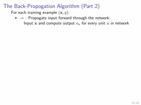
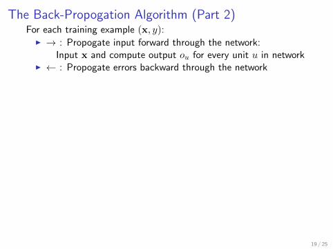
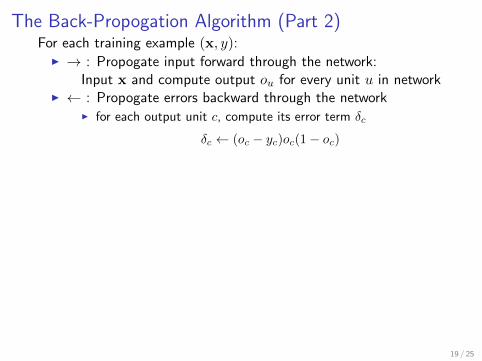
The Back-Propogation Algorithm (Part 2)For each training example (x, y):

I → : Propogate input forward through the network:Input x and compute output ou for every unit u in network

I ← : Propogate errors backward through the networkI for each output unit c, compute its error term δc

δc ← (oc − yc)oc(1− oc)

I for each hidden unit h, compute its error term δh

δh ←

∑i∈succ(h)

wihδi

oh(1− oh)

I update each weight wji

wji ← wji − αδjxji

I xji: input from unit i into j(oi if i is hidden unit; xi if i is an input)

I wji: weight from unit i to unit j

19 / 25



I ← : Propogate errors backward through the network

I for each output unit c, compute its error term δc



δh ←

∑i∈succ(h)

wihδi

oh(1− oh)





19 / 25






δh ←

∑i∈succ(h)

wihδi

oh(1− oh)





19 / 25






δh ←

∑i∈succ(h)

wihδi

oh(1− oh)





19 / 25






δh ←

∑i∈succ(h)

wihδi

oh(1− oh)





19 / 25






δh ←

∑i∈succ(h)

wihδi

oh(1− oh)




I wji: weight from unit i to unit j19 / 25

Derivation of Back-Propagation

I For simplicity, assume online learning (vs. batch learning):1-step grad. descent after seeing ea. training example (x, y)

I For each (x, y) the error is

E(w) =1

2

k∑c=1

(oc − yc)2

I oc: the c-th output unit (when input is x)I yc: the c-th element of label indicator vector

I Use grad. descent to change all weights wji to minimize error.I Separate into two cases:

I Case 1: wji when j is output unitI Case 2: wji when j is hidden unit

20 / 25

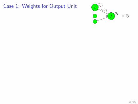
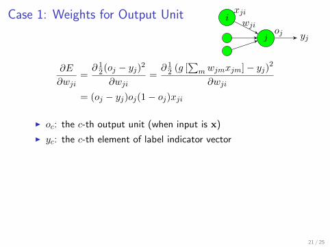
Case 1: Weights for Output Unit ixji

joj yj

wji

∂E

∂wji=∂ 12(oj − yj)2

∂wji=∂ 12 (g [

∑mwjmxjm]− yj)2

∂wji

= (oj − yj)oj(1− oj)xji

I oc: the c-th output unit (when input is x)

I yc: the c-th element of label indicator vector

I grad. descent: to min. error, head away from part. derivative:

wji ← wji − α∂E

∂wji= wji − α(oj − yj)oj(1− oj)xji

21 / 25


joj yj

wji

∂E

∂wji=∂ 12(oj − yj)2

∂wji=∂ 12 (g [

∑mwjmxjm]− yj)2

∂wji







21 / 25


joj yj

wji

∂E

∂wji=∂ 12(oj − yj)2

∂wji=∂ 12 (g [

∑mwjmxjm]− yj)2

∂wji







21 / 25


joj yj

wji

∂E

∂wji=∂ 12(oj − yj)2

∂wji=∂ 12 (g [

∑mwjmxjm]− yj)2

∂wji







21 / 25


joj yj

wji

∂E

∂wji=∂ 12(oj − yj)2

∂wji=∂ 12 (g [

∑mwjmxjm]− yj)2

∂wji







21 / 25

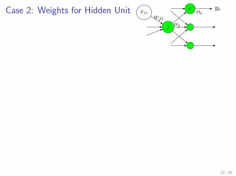
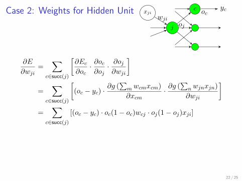
Case 2: Weights for Hidden Unit ycc oc

j

xji

ojwji

∂E

∂wji=

∑c∈succ(j)

[∂Ec

∂oc· ∂oc∂oj· ∂oj∂wji

]

=∑

c∈succ(j)

[(oc − yc) ·

∂g (∑

mwcmxcm)

∂xcm·∂g (

∑nwjnxjn)

∂wji

]=

∑c∈succ(j)

[(oc − yc) · oc(1− oc)wcj · oj(1− oj)xji]

22 / 25


j

xji

ojwji

∂E

∂wji=

∑c∈succ(j)

[∂Ec


]

=∑

c∈succ(j)

[(oc − yc) ·

∂g (∑

mwcmxcm)

∂xcm·∂g (

∑nwjnxjn)

∂wji

]=

∑c∈succ(j)


22 / 25


j

xji

ojwji

∂E

∂wji=

∑c∈succ(j)

[∂Ec


]

=∑

c∈succ(j)

[(oc − yc) ·

∂g (∑

mwcmxcm)

∂xcm·∂g (

∑nwjnxjn)

∂wji

]

=∑

c∈succ(j)


22 / 25


j

xji

ojwji

∂E

∂wji=

∑c∈succ(j)

[∂Ec


]

=∑

c∈succ(j)

[(oc − yc) ·

∂g (∑

mwcmxcm)

∂xcm·∂g (

∑nwjnxjn)

∂wji

]=

∑c∈succ(j)


22 / 25

Neural Network Learning Issues: Weights

I When to terminate back-prop.? Overfitting and early-stoppingI After fixed number of iterations (ok)I When training error less than a threshold (not ok!)I When holdout set error starts to go up (ok)

I Local Optima:I Weights will converge to local minimum

I Learning Rate:I Convergence sensitive to learning rateI Weight learning can be slow

23 / 25

slide 30

Sensitivity to learning rate

From J. Hertz, A. Krogh, and R. G. Palmer. Introduction to the Theory of Neural Computation. Addison-Wesley, 1994.

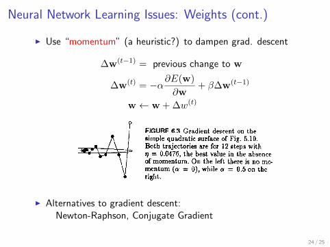
Neural Network Learning Issues: Weights (cont.)

I Use “momentum” (a heuristic?) to dampen grad. descent

∆w(t−1) = previous change to w

∆w(t) = −α∂E(w)

∂w+ β∆w(t−1)

w← w + ∆w(t)

I Alternatives to gradient descent:Newton-Raphson, Conjugate Gradient

24 / 25

Neural Network Learning Issues: Structure

I How many hidden units?

I How many layers?

I How to connect units?

I Cross validation

25 / 25

Documents

Perceptrons and Neural Networkspages.cs.wisc.edu/~bgibson/cs540/handouts/neural.pdf · Outline I Perceptron: a single neuron I Linear perceptron I Non-linear perceptron I Learning