Neural Networks for Classifying Probability Distributions

NIST Technical Note 2152

Neural Networks for Classifying Probability Distributions

Siham KhoussiAlan Heckert

Abdella BattouSaddek Bensalem

This publication is available free of charge from: https://doi.org/10.6028/NIST.TN.2152

NIST Technical Note 2152

Neural Networks for Classifying Probability Distributions

Siham KhoussiAbdella Battou

Advanced Network Technologies DivisionInformation Technology Laboratory

Alan HeckertStatistical Engineering Division

Information Technology Laboratory

Saddek BensalemUniversity of Grenoble Alpes (UGA)

Grenoble, France


April 2021

U.S. Department of CommerceGina M. Raimondo, Secretary

National Institute of Standards and TechnologyJames K. Olthoff, Performing the Non-Exclusive Functions and Duties of the Under Secretary of Commerce

for Standards and Technology & Director, National Institute of Standards and Technology

Certain commercial entities, equipment, or materials may be identified in this document in order to describean experimental procedure or concept adequately. Such identification is not intended to imply

recommendation or endorsement by the National Institute of Standards and Technology, nor is it intended toimply that the entities, materials, or equipment are necessarily the best available for the purpose.

National Institute of Standards and Technology Technical Note 2152 Natl. Inst. Stand. Technol. Tech. Note 2152, 20 pages (April 2021)

CODEN: NTNOEF


Abstract

Probability distribution fitting of an unknown stochastic process is an important prelim-inary step for any further analysis in science or engineering. However, it requires somebackground in statistics, prior considerations of the process or phenomenon under studyand familiarity with several distributions. As such, this paper presents an alternative ap-proach which doesn’t require prior knowledge of statistical methods nor previous assump-tion on the available data. Instead, using Deep Learning, the best candidate distribution isextracted from the output of a neural network that was previously trained on a large suitabledatabase in order to classify an array of observations into a matching distributional model.We find that our classifier can perform this task comparably to using maximum likelihoodestimation with an Anderson-Darling goodness of fit test.

Key words

Deep Learning; neural networks; distribution fitting; data normalization.

1

______________________________________________________________________________________________________ This publication is available free of charge from

: https://doi.org/10.6028/NIST.TN

.2152

Table of Contents1 Introduction 12 Related work 23 Methodology 3

3.1 Data collection 33.2 Neural networks 53.3 Evaluation 7

4 Results 75 Conclusion 116 Limitations 137 Future work 13References 14

List of TablesTable 1 Confusion matrix for the large category: NN vs maximum likelihood/Anderson-

Darling (MLE-AD) 11Table 2 Confusion matrix for the moderate category: NN vs maximum likelihood/Anderson-

Darling (MLE-AD) 12Table 3 Confusion matrix for the small category: NN vs maximum likelihood/Anderson-

Darling (MLE-AD) 12

List of FiguresFig. 1 Traditional approach of conducting distribution fitting 1Fig. 2 DEX mean plot for small sample sizes 9Fig. 3 DEX mean plot for moderate sample sizes 10Fig. 4 DEX mean plot for large sample sizes 10

2



.2152

1. Introduction

Many problems in both science and engineering require fitting a distributional model to auni-variate dataset. That is, data consisting of a set of N empirical observations obtainedby measuring a certain system, provided that the measurements are independent and comefrom the same distribution.

Distributional modeling can be used in several contexts. Statistical tests typically de-pend on certain assumptions with regards to the underlying distribution (e.g., many testsare based on the assumption of normality). Appropriate distributional models are also usedto more accurately assess uncertainty and, in particular, to assess the uncertainty over thefull range of the data. Although a poorly chosen distributional model may suffice for mea-suring and assessing the uncertainty of averages, this will not be the case for tails of thedistribution. In many applications (e.g., reliability), accurate assessment of the tail behavioris more critical than the average. Obtaining an appropriate distributional model can be anexhaustive process that takes time, patience and requires previous knowledge of statisticsand is, therefore, a difficult task for some analysts.

Fig. 1. Traditional approach of conducting distribution fitting

Figure 1 presents the traditional approach to obtaining an appropriate distributionalmodel. This approach consists of four steps: The first step is to assess whether the data isin fact independent. This can be done via standard statistical tests for randomness or auto-correlation (e.g., runs test, Ljung-Box test). It can also be assessed graphically (e.g., a lagplot or an auto-correlation plot). The second step is to identify potential distributional mod-els. Typically, histograms or kernel density plots are used to help identify the basic shapeof the underlying distribution as well as certain properties such as the skewness and thepresence of multiple modes in the data. Identifying good potential models from these plotstypically requires some degree of statistical knowledge, experience and familiarity with

1



.2152

several distributions. The third step is to estimate the parameters of the chosen distributionvia methods like maximum likelihood. The fourth and final step is to assess the goodnessof fit of the proposed distributional model via one of the many goodness of fit tests suchas the Anderson-Darling test, the Kolmogorov-Smirnov test, the Cramer-Von Mises test orinformation criteria such as AIC and BIC.

This research focuses on the use of Deep Learning (DL) to assist in identifying thebest distributional model among a fixed set of candidate models (step 2) in order to helpanalysts who are not equipped with sufficient statistical background easily map a set ofempirical observations obtained from an experiment to an appropriate distributional model.DL is a sub-field of machine learning that applies neural network architectures to learnfeatures of the object to be classified. It has become more popular in recent years dueto its high accuracy, its capacity to deal with massive data and larger neural networks aswell as its capability to deduce data features automatically. Although DL neural networkstake a longer duration to train and usually require high performance servers with graphicprocessing units (GPU) which are expensive, it is still considered an efficient and effectiveapproach for object classification.

The approach proposed here exploits the strengths of Deep Learning for classificationof distributional models. We restrict ourselves to the case of continuous measurementswhere the data is not binned, censored or truncated. Moreover, we do not consider patho-logical distributions (e.g. Cauchy distribution). In this paper, we train a feed forward neuralnetwork to recognize patterns in an input dataset then predict the ”best” candidate modelfrom nine commonly used distributions that are widely encountered. The distributions con-sidered in this study are: uniform, normal, logistic, exponential, half normal, half logistic,gumbel max, gumbel min and double exponential. Note that once the DL has identifiedthe ”best” distributional model (step 2 according to Figure 1), the parameter estimation andthe goodness of fit assessment still need to be applied using traditional statistics. Although,in this study a limited list of distributions is examined, it is covering the most encoun-tered models. Moreover, this paper is intended to serve as a proof of concept to prove theviability of our method then increase the number of the distributions later on.

In this paper, we present similar related works in section 2. We explain our methodol-ogy and evaluation metrics in section 3. The results of our analysis are shown in section 5.We also discuss the limitations of this work in section 6 and finally preview our ongoingand future research in Section 7.

2. Related work

There have been several attempts to automate the distributional modeling process by cre-ating software and packages that let the user know the “best” candidate distribution thatmatches their inputs. Generally, most of them use traditional statistical techniques to pre-process data and run some goodness of fit tests in order to rank and identify a good repre-sentation of the data. Similar tools and packages include [1], [2] and [3], etc. All of themhave the same goal which is to guide and help analysts regardless of their knowledge of

2



.2152

statistics, pin down the best candidate distribution matching their data and avoid using thewrong distribution while saving them time.

Other researchers in the literature investigated the use of neural network for conductingparameter estimation of probability density functions which corresponds to step 3 fromFigure 1. Similar papers include [4], [5] and [6]. Others have discussed conditional densityestimation using artificial intelligence such as [7] and [8]. Additionally, [9] presented thebest practices for conditional density estimation for finance applications, specifically, andusing neural networks. Finally, [10] used an ensemble of mixture density networks topredict the probability density function of the surf height in order to know if it will fallwithin a given ‘surfable’ range. However, at the time of this writing, there has been nowork involving the use of neural network to tackle step 2 of Figure 1 and create a classifierfor distributional models based on a set of independent empirical observations. In fact, thistask is the most important since one it is completed and the exact distribution model hasbeen identified, it becomes extremely easy to estimate the parameters of the distributionand formulate the probability density function (PDF).

3. Methodology

3.1 Data collection

In this paper, we collected data in two stages. The first stage was to create the datasets fortraining and validating the neural networks.

Probability distributions are characterized by three types of parameters: a location,a scale and one or more shape parameters. The standard form of the distribution is thecase where the location parameter is zero and the scale parameter is one. Given a graphof the standard form of the probability density function, the effect of a non-zero locationparameter is to shift the graph left (for negative location values) or right (for positive lo-cation values) on the horizontal axis. The effect of a scale parameter is to either stretchthe graph on the horizontal axis (for scale parameters greater than one) or to compress thegraph on the horizontal axis (for scale parameters less than one). Chapter one from theNIST/SEMATECH e-Handbook [11] shows examples of this for the normal distribution.The relationship of the probability density function of a general form of the distribution(i.e., location and scale not equal to zero and one) is:

f (x;a,b) =f ( (x−a)

b ;0,1)b

(1)

where a and b are the location and scale parameters, respectively. Any parameter that isnot either a location or scale (or a parameter that is a function of the location and scaleparameters only) is considered a shape factor. Shape parameters allow a distribution totake a variety of different shapes. By shape, we mean properties such as skewness andkurtosis (peakedness). Location and scale parameters have no effect on these properties.For this study, we only considered distributions without shape parameters and keep the ones

3



.2152

with the location and scale factors. Since the shape of the distribution does not depend onthe location and scale parameters, the training data only utilized the standard form of thedistributions (location = 0, and scale = 1).

For each of the nine distributions considered in this study, 10,000 datasets were gener-ated for the standard form of the distributions at different sample sizes (30, 50, 100, 250,500, 750, 1,000 and 10,000). The random numbers were generated with the Dataplot soft-ware [12]. And a congruential-Fibonnaci [13] generator was used with a different seedfor each distribution/sample size configuration. For each set of random numbers, a kerneldensity plot was generated with Dataplot using the Silverman algorithm [14]. The kerneldensity plot is a graphical estimate of the underlying probability density function and isconsidered a typical technique by statisticians to conduct exploratory analysis of data in or-der to identify the shape of the underlying distributional model. Furthermore, the intuitionbehind the choices of the sample sizes is based on the fact that the smoothness of the kerneldensity plot increases with the increase of the number of available data points. In this study,several experiments were conducted to assess and select the correct sample sizes prior totraining the neural networks that will eventually determine if the underlying distributioncan be recognized from the kernel density plot.

The kernel density estimate, fn(x), of a set of n points from a density f is defined as:

fn(x) =∑

nj=1 K (x−X j)

h nh

(2)

where K is the kernel function and h is the smoothing parameter or window width. TheSilverman algorithm uses a Gaussian kernel function. This down weights points smoothlyas the distance from x increases. We used Silverman’s default recommendation for the hparameter:

0.9min(s, IQ/1.34)n−1/5 (3)

with s, IQ, and n denoting the sample standard deviation, the sample interquartile rangeand the sample size, respectively. The kernel density plot was generated at 256 points.The input for the neural networks is the y-axis coordinates of the kernel density plot. Theimplicit x-axis coordinates are 1, 2, ..., 256.

The second stage was to create datasets for testing. Typically, real world data willhave location and scale values, so we generated random numbers for each distribution withseveral different location and scale parameters. Specifically, datasets were generated withsample sizes of 50, 100, 250, 500, 750, 1,000 and 10,000. For each sample size, datasetswere generated with location values: 20, 60 and 100 and scale values: 10, 30 and 50. Thisadds up to a total of nine different combinations of location and scale parameters. Then,we generated 1,000 datasets for each distribution/sample size/location/scale combination.

As with the training data, kernel density plots were generated for each dataset. And thealgorithm used for creating the kernel density plots in the training data, was also used forthis set.

4



.2152

One question of interest is whether an appropriate normalization can address the issuesintroduced by the location and scale parameters. The training and the validation data wasgenerated for standard forms of the distributions (location parameter = 0, scale parameter =1) while the testing data was generated with non-standard values of the location and scaleparameters. The y-coordinate (height) of the kernel density plots is used for the input to theneural networks (NN) which gives an implicit x-coordinate scale of 1 to 256. The locationparameter does not change the height of the kernel density. However, the scale parameterdoes change the height of the kernel density plot.

Using an implicit x-axis scale of 1 to 256 for both the training and testing data shouldminimize the effects of the location parameter. However, since the scale parameter changesthe height of the kernel density plot, there is a need to transform the kernel density heightsso that the testing data can be more effectively compared to the training and validation data.

In this study, we experimented with several transformation algorithms on both the train-ing/validation and the testing data. But, only two yielded promising results:

1. The U-score, also referred to as the Min-Max normalization. The u-score algorithmtransforms the kernel density heights to a (0,1) scale according to the following math-ematical formulation:

u score =x−min(x)

max(x))−min(x)(4)

where x is the original value, u score is the normalized value, min(x) and max(x) arerespectively the minimum and maximum values of each dataset x.

2. The kernel density normalization transforms the kernel density heights to integrateto 1 on the 1 to 256 x-coordinate scale:

k score =x

∑256i=1 xi

(5)

where x is the original value and k score is the normalized value.

3.2 Neural networks

An initial attempt at producing a single solid neural network model to classify an arbitrarynumber of data points (N) to a matching probability density function (PDF) has not yieldedpromising results especially when N is small. The intuition behind the misclassificationcould be interpreted as follows: our approach relies on building a kernel density estimator(KDE) from a set of independent empirical observations. This KDE tends to be noisyfor small N and becomes increasingly smooth as N gets larger. Thus, models trained onthe larger sample sizes perform poorly on the smaller sample sizes and models trained onsmaller sample sizes perform poorly for larger sample sizes.

To improve performance, we consider 20+ models. The data collected is generatedusing eight sample sizes: N=30, N=50, N=100, N=250, N=500, N=750, N=1,000 and

5



.2152

N=10,000 and each model is trained on a specific sample size range. The idea is to eval-uate the models individually and collectively to deduce which ones work best for small,moderate and large sample sizes. Examples of the considered models include: Model 1(N ∈ [30,100]), Model 2 (N ∈ [100,750]), Model 3 (N ∈ [750,10000]), etc.

All the models have the same input and output layers. However, their hidden layersdiffer in size and width. The input layer has 256 unit representing the Y-Axis coordinatesfor a kernel density plot whereas the output layer has 9 points which refer to the one hotencoding of the 9 distributional models considered in this paper. For each interval, westarted with a very simple Feed Forward Neural Network (FNN) that overfits. We thenproceeded to handle the overfiting by tuning FNN parameters to achieve the lowest lossand highest accuracy. We found that the following work best:

1. 20% of the training data was allocated for the validation;

2. All models use Softmax as the activation function for the output layer and Relu forthe hidden layers;

3. The choice of the loss function was Categorical cross-entropy (CAT) for larger inter-vals and Mean squared error (MSE) for smaller intervals;

4. The ADAM optimizer was used when the loss function was set to CAT and RMSpropfor MSE;

5. The learning rate is set to 1e-6 or 1e-5 in most cases;

6. The batch size is set to 200 for most models;

7. Each model was run for an average epoch of 500;

8. The weights were initialized using the ’He uniform’ distribution;

9. The bias was enabled in the hidden layers and disabled in the output layer;

10. The depth of each NN model was 40, while the width was either 512 or 1024 nodesper layer;

11. Early stopping was deployed;

12. Regularized and dropout were used.

The models were all implemented using Python and Keras with Tensorflow as a back-end and the experiment was run on our testbed with with 1 GPU and 40 CPU cores.

6



.2152

3.3 Evaluation

After the training and validation steps of the neural networks were complete, additionaldatasets were used to test the models (stage 2 from section 3.1). Furthermore, to deter-mining the viability and effectiveness our approach, the models’ accuracy results werecompared against the results of a conventional statistical approach as follows:

• The data is fit to each distribution using maximum likelihood (MLE). The one ex-ception is that the half-logistic distribution is fit using the method of moments.

• After estimating the parameters with maximum likelihood, the distributions are rankedbased on the Anderson-Darling (AD) goodness of fit statistic [15]. The AD test isa refinement of the Kolmogorov-Smirnov (KS) statistic that puts more weight in thetails of the distribution. The AD test is generally considered to have more power thanthe the KS test.

Given an ordered set of data Yi and a cumulative distribution function F , the Anderson-Darling test statistic is defined as

A2 =−N−N

∑i=1

(2i−1)N

[lnF(Yi)+ ln(1−F(YN+1−i))] (6)

There are a variety of estimation methods and goodness of fit statistics that could beused for this approach. However, the combination of MLE estimation and ranking bythe AD goodness of fit test provides a reasonable benchmark for assessing the results ofthe neural networks. Moreover, it is important to mention that both approaches (neuralnetworks and MLE-AD) were compared based on the same data.

4. Results

Our primary metric of success was the percentage of times that the correct distributionwas accurately identified. For the mis-classified cases, we also identify which distributionswere chosen instead. The following factors are examined while analyzing the results:

• There are two different normalization algorithms considered. These are referred toas the u-score and the kernel density normalization, respectively (section 3.1);

• There were eight different sample sizes used for the testing datasets. We groupedthese into three categories: ”small”, that is datasets with 30 or 50 or 100 observations;”moderate”, that is datasets with 100, 250, 500 or 750 observations; and ”large”, thatis datasets with 750, 1,000 or 10,000 observations. Note that these categories containoverlaps in order to create three intervals: small [30,100], moderate [100,750] andlarge [750,10000]. These intervals are useful because real world data is not confinedto these particular eight sizes;

7



.2152

• This study considered nine distinct distributions. These distributions allow for loca-tion and scale parameters, but none of them have shape parameters;

• There were 20+ training models considered;

• There were nine combinations of location/scale parameters for each distribution/samplesize cell.

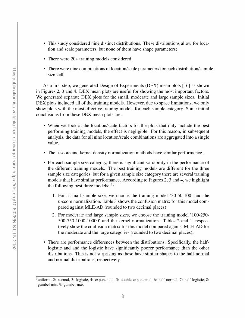
As a first step, we generated Design of Experiments (DEX) mean plots [16] as shownin Figures 2, 3 and 4. DEX mean plots are useful for showing the most important factors.We generated separate DEX plots for the small, moderate and large sample sizes. InitialDEX plots included all of the training models. However, due to space limitations, we onlyshow plots with the most effective training models for each sample category. Some initialconclusions from these DEX mean plots are:

• When we look at the location/scale factors for the plots that only include the bestperforming training models, the effect is negligible. For this reason, in subsequentanalysis, the data for all nine location/scale combinations are aggregated into a singlevalue.

• The u-score and kernel density normalization methods have similar performance.

• For each sample size category, there is significant variability in the performance ofthe different training models. The best training models are different for the threesample size categories, but for a given sample size category there are several trainingmodels that have similar performance. According to Figures 2, 3 and 4, we highlightthe following best three models: 1:

1. For a small sample size, we choose the training model ’30-50-100’ and theu-score normalization. Table 3 shows the confusion matrix for this model com-pared against MLE-AD (rounded to two decimal places);

2. For moderate and large sample sizes, we choose the training model ’100-250-500-750-1000-10000’ and the kernel normalization. Tables 2 and 1, respec-tively show the confusion matrix for this model compared against MLE-AD forthe moderate and the large categories (rounded to two decimal places);

• There are performance differences between the distributions. Specifically, the half-logistic and and the logistic have significantly poorer performance than the otherdistributions. This is not surprising as these have similar shapes to the half-normaland normal distributions, respectively.

1uniform, 2: normal, 3: logistic, 4: exponential, 5: double-exponential, 6: half-normal, 7: half-logistic, 8:gumbel-min, 9: gumbel-max

8



.2152

• As expected, performance improves as the sample size increases. According to theDEX mean plots, for the small category, the overall performance was approximately70%, for the moderate category the overall performance was close to 85%, and forthe large category the overall performance was about 98%. The latter means thatwith a large number of observations, our NN can identify ”the correct” distribution.

Distribution TrainingMethod

NormalizationMethod

uscore kernel

Location Scale

30

40

50

60

70

80

90

100

Dex Mean Plot for Small Sample Sizes (50, 100), Best Training Models

ME

AN

PE

RC

EN

T C

OR

RE

CT

CL

AS

SIF

ICA

TIO

N

Training Models

30-50

30-50-100

50-100-250

30-50-100-250

50-100-250-500

100-250

50-100-250

50-100-250-500-750-1000-10000

100-250-500-750-1000-10000

ML-AD

Distributions

Double Exponential

Exponential

Half-Logistic

Half-Normal

Logistic

Gumbel (Max)

Gumbel (Min)

Normal

Uniform

Fig. 2. DEX mean plot for small sample sizes

9



.2152


NormalizationMethod

uscore kernel

Location Scale

60

70

80

90

100

Dex Mean Plot for Moderate Sample Sizes (100, 250, 500, 750), Best Training Models

ME

AN

PE

RC

EN

T C

OR

RE

CT

CL

AS

SIF

ICA

TIO

N

Training Models

50-100-250

30-50-100-250

50-100-250-500

100-250

50-100-250

250-500-750-1000-10000

50-100-250-500-750-1000-10000

100-250-500-750-1000-10000

ML-AD

Distributions

Double Exponential

Exponential

Half-Logistic

Half-Normal

Logistic

Gumbel (Max)

Gumbel (Min)

Normal

Uniform

Fig. 3. DEX mean plot for moderate sample sizes


NormalizationMethod

uscore kernel

Location Scale

93

94

95

96

97

98

99

100

Dex Mean Plot for Larger Sample Sizes (750, 1000, 10000), Best Training Models

ME

AN

PE

RC

EN

T C

OR

RE

CT

CL

AS

SIF

ICA

TIO

N

Training Models

1000-10000

750-1000-10000

500-750-1000-10000

250-500-750-1000-10000

50-100-250-500-750-1000-10000

100-250-500-750-1000-10000

ML-AD

Distributions

Double Exponential

Exponential

Half-Logistic

Half-Normal

Logistic

Gumbel (Max)

Gumbel (Min)

Normal

Uniform

Fig. 4. DEX mean plot for large sample sizes

10



.2152

Table 1. Confusion matrix for the large category: NN vs maximum likelihood/Anderson-Darling(MLE-AD)

Selected distributionTrue

Distribution Approach 1 2 3 4 5 6 7 8 9

NN 100.00 0.00 0.00 0.00 0.00 0.00 0.00 0.00 0.00Uniform MLE-AD 99.99 0.00 0.00 0.00 0.00 0.00 0.00 0.00 0.00

NN 0.00 96.77 3.20 0.00 0.00 0.00 0.00 0.01 0.02Normal MLE-AD 0.00 96.38 3.62 0.00 0.00 0.00 0.00 0.00 0.00

NN 0.00 1.87 96.94 0.00 1.13 0.00 0.00 0.03 0.03Logistic MLE-AD 0.00 0.79 99.08 0.00 0.12 0.00 0.00 0.00 0.01

NN 0.00 0.00 0.00 98.93 0.00 0.00 1.07 0.00 0.00Exponential MLE-AD 0.00 0.00 0.00 99.93 0.00 0.00 0.06 0.01 0.00

NN 0.00 0.00 0.30 0.00 99.70 0.00 0.00 0.00 0.00Double Exponential MLE-AD 0.00 0.00 0.34 0.00 99.64 0.00 0.00 0.01 0.00

NN 0.00 0.00 0.00 0.00 0.00 96.45 3.55 0.00 0.00Half Normal MLE-AD 0.00 0.00 0.00 0.00 0.00 99.57 0.34 0.00 0.09

NN 0.00 0.00 0.00 2.32 0.00 2.47 95.21 0.00 0.00Half Logistic MLE-AD 0.00 0.00 0.00 0.81 0.00 5.70 93.48 0.00 0.01

NN 0.00 0.00 0.00 0.00 0.00 0.00 0.00 100.00 0.00Gumbel Min MLE-AD 0.00 0.00 0.00 0.00 0.01 0.00 0.00 99.99 0.00

NN 0.00 0.00 0.00 0.01 0.00 0.00 0.01 0.00 99.98Gumbel Max MLE-AD 0.00 0.00 0.00 0.00 0.00 0.00 0.00 0.01 99.99

For evaluation purposes, we also provide confusion matrices for MLE-AD in the sametables as the output of the Neural Networks (NN) (tables 1, 2 and 3). Theses tables indicatesthat neural networks perform comparably to MLE-AD and give better performance in amajority, but not all, of the cases, than the MLE-AD method. In fact:

• For the small category, DL outperforms MLE-AD for 6 out of 9 distributions andthey perform essentially the same for the half-logistic distribution;

• For the moderate category, DL outperforms MLE-AD for 6 out of the 9 distributionsand they perform essentially the same for the Gumbel max distribution;

• For the large category, ML-AD performs slightly better for 3 distributions, DL per-forms slightly better for one distribution and for the remaining 5 distributions theyperform essentially the same.

5. Conclusion

In this empirical study, we investigated the use of neural networks for distributional mod-els classification. Given a set of independent empirical observations obtained from anunknown process or phenomenon, we show that a neural network classifier is capable ofidentifying which distributional model is best fitted for the input data.

11



.2152

Table 2. Confusion matrix for the moderate category: NN vs maximumlikelihood/Anderson-Darling (MLE-AD)



NN 99.95 0.03 0.00 0.00 0.00 0.00 0.00 0.02 0.01Uniform MLE-AD 73.78 15.48 0.07 0.00 0.00 0.94 0.00 5.30 4.43

NN 0.10 91.01 7.08 0.00 0.34 0.00 0.00 0.74 0.72Normal MLE-AD 0.00 79.27 18.55 0.00 0.38 0.00 0.00 0.93 0.86








Table 3. Confusion matrix for the small category: NN vs maximum likelihood/Anderson-Darling(MLE-AD)



NN 97.44 0.89 0.00 0.01 0.00 0.73 0.02 0.58 0.33Uniform MLE-AD 3.72 52.00 0.64 0.00 0.00 2.68 0.01 21.72 19.24

NN 1.99 64.13 17.94 0.00 4.04 0.46 0.00 5.89 5.54Normal MLE-AD 0.00 51.72 31.96 0.00 3.07 0.00 0.00 6.81 6.44








12



.2152

We chose two neural networks models depending on the number of available data points(small, moderate and large) and apply a suitable normalization technique (kernel densitynormalization or u-score normalization) then run the points through the neural networks topredict the ”best fitted” distributional model.

We validated the results by comparing them to a traditional statistical approach: pa-rameter estimation by maximum likelihood with subsequent goodness of fit ranking byAnderson-Darling (MLE-AD) and showed that this approach outperforms MLE-AD in amajority of cases.

6. Limitations

In this study we proposed the use of deep learning to build a classifier for distributionalmodeling. This classifier takes as input a set of data points and provides a distribution labelthat matches one of nine most common distributions.

This approach is not a complete replacement of the traditional statistical methodol-ogy that statisticians have been following to analyze and fit the data. However, it is analternative to step 2 from Figure 1 (Exploratory analysis) which usually requires a goodbackground of statistical knowledge as well as a familiarity with several distributions to beable to recognize a good potential distribution from a set of empirical observations. Thisis typically done via histograms or kernel density plots to help pin down the basic shapeof the underlying distribution and find properties such as the skewness and the presence ofmultiple modes in the data.

Moreover, this paper considers uni-variate non-censored and non-truncated data anddoesn not consider families of distributions with the shape parameters or noisy data whichis generally a mixture distributions. In this research, We consider a limited number of dis-tributions that correspond to the most commonly used models that are widely encountered.The reason behind our decision is that we hope to provide an initial working prototype thatcan prove the viability and applicability of our methodology.

7. Future work

In future work, we will extend the training set beyond the nine currently supported distri-butions. In particular, this will include commonly used families of distributions such asthe Weibull, lognormal and gamma distributions. These families can generate a variety ofshapes based on the value of their shape parameter. For this reason, we plan to incorporatethe ability to make more specific classifications (e.g., distinguish between a Weibull or alognormal distribution) and compare this to approaches such as the likelihood ratio test[17], [18].

Furthermore, we are currently building a tool that automates the distributional fittingprocess for uncensored and unbinned uni-variate data that deploys our trained neural net-works to identify the best candidate model from the distributions presented in this study.

13



.2152

This tool takes empirical observation of any size and computes the kernel density estima-tion on behalf of the user, then runs the classifier to predict the best fit distribution.

In addition to that, we are also deploying traditional statistical techniques to estimatethe parameters of the fitted distribution and assess it’s goodness of fit by comparing thepredictions to Anderson Darling, Kolmogorov-Smirnov and the probability plot correlationcoefficient tests as well as information criteria (AIC, BIC).

Moreover, we include in the tool an interactive module to clean and pre-process the databefore starting the NN classifier. This module will contain a step by step guide to help usersidentify and eventually remove outliers prior to running the neural network classification.It is very important because outlier identification is for the purpose of identifying bad datain the sense of being erroneous (e.g., data is mis-coded or there is an assignable cause forwhy the observation is in error). Furthermore, statistical classification of an observationas an outlier is dependent on the underlying distribution of the data, which is what we aretrying to determine, so simply being an ”extreme” observation is not sufficient justificationfor removing it.

References

[1] Delignette-Muller M, Dutang C (2015) fitdistrplus: An R Package for Fitting Distri-butions. Journal of Statistical Software 64(4):1–34.

[2] Law AM, McComas MG (2011) How the ExpertFit distribution-fitting software canmake your simulation models more valid. Proceedings of the Winter Simulation Con-ference 1:199–204.

[3] Schittkowski K (2002) EASY-FIT: a software system for data fitting in dynamicalsystems. Structural and Multidisciplinary Optimization 23:153–169.

[4] Reyneri L, Colla V, Vannucci M (2011) Estimate of a probability density functionthrough neural networks 6691(1):57–64.

[5] Likas A (2001) Probability density estimation using artificial neural networks. Com-puter Physics Communications 135:167–175.

[6] Nakamura Y, Hasegawa O (2017) Non parametric density estimation based on self-organizing incremental neural network for large noisy data. IEEE Transactions onNeural Networks and Learning Systems 28(1):8–17.

[7] Kobyz GV, Zamyatin AV (2015) Conditional probability density estimation using ar-tificial neural network :441–445.

[8] Wesley Tansey KP, Scott JG (2016) Better Conditional Density Estimation for NeuralNetworks Available at https://arxiv.org/abs/1606.02321.

[9] Rothfuss J, Ferreira F, Walther S, Ulrich M (2019) Conditional Density Estimationwith Neural Networks: Best Practices and Benchmarks Available at http://arxiv.org/abs/1903.00954.

[10] Carney CP Michael, Dowling J, Lee C (2005) Predicting probability distributions forsurf height using an ensemble of mixture density networks :113–120.

[11] Filliben JJ (2003) NIST/SEMATECH e-Handbook of Statistical Methods,

14



.2152

https://arxiv.org/abs/1606.02321

http://arxiv.org/abs/1903.00954

http://arxiv.org/abs/1903.00954

Chapter 1 (National Institute of Standards and Technology), . Available athttp://web.archive.org/web/20191213225442/https://www.itl.nist.gov/div898/handbook/eda/section3/eda364.htm.

[12] Filliben JJ, Heckert AN (1978) Dataplot (National Institute of Standards and Tech-nology), . Available at http://web.archive.org/web/20190819195854/https://www.itl.nist.gov/div898/software/dataplot/.

[13] David Kahaner GEFSNMAM Cleve B Moler (1988) Numerical Methods and Soft-ware, . Available at https://books.google.com/books/about/Numerical Methods and Software.html?id=jipEAQAAIAAJ.

[14] Silverman BW (1982) Kernel Density Estimation Using the Fast Fourier Transform,. Available at https://rss.onlinelibrary.wiley.com/doi/epdf/10.2307/2347084.

[15] Stephens MA (1974) EDF Statistics for Goodness of Fit and Some Comparisons.Journal of the American Statistical Association 69(347):730.

[16] Filliben JJ (2003) Mean Plot (National Institute of Standards and Technology),. Available at http://web.archive.org/web/20180217195200/http://www.itl.nist.gov/div898/handbook/eda/section3/dexmeanp.htm.

[17] Dumonceaux R, Antle CE, Haas G (1973) Likelihood Ratio Test for discriminationbetween two models with unknown scale and location parameters. Technometrics15(1):19.

[18] Dumonceaux R, Antle CE (1973) Discrimination Between the Log-Normal and theWeibull Distributions. Technometrics 15(4):923–926.

15



.2152

http://web.archive.org/web/20191213225442/https://www.itl.nist.gov/div898/handbook/eda/section3/eda364.htm

http://web.archive.org/web/20191213225442/https://www.itl.nist.gov/div898/handbook/eda/section3/eda364.htm

http://web.archive.org/web/20190819195854/https://www.itl.nist.gov/div898/software/dataplot/

http://web.archive.org/web/20190819195854/https://www.itl.nist.gov/div898/software/dataplot/

https://books.google.com/books/about/Numerical_Methods_and_Software.html?id=jipEAQAAIAAJ

https://books.google.com/books/about/Numerical_Methods_and_Software.html?id=jipEAQAAIAAJ

https://rss.onlinelibrary.wiley.com/doi/epdf/10.2307/2347084

http://web.archive.org/web/20180217195200/http://www.itl.nist.gov/div898/handbook/eda/section3/dexmeanp.htm

http://web.archive.org/web/20180217195200/http://www.itl.nist.gov/div898/handbook/eda/section3/dexmeanp.htm

Documents

Neural Networks for Classifying Probability Distributions