Neural Networks for Time Series

Processing

Georg Dor�ner

Dept� of Medical Cybernetics and Arti�cial Intelligence

University of Vienna

and Austrian Research Institute for Arti�cial Intelligence

Abstract

This paper provides an overview over the most common neural network types for

time series processing� i�e� pattern recognition and forecasting in spatio�temporal

patterns� Emphasis is put on the relationships between neural network models

and more classical approaches to time series processing� in particular� forecasting�

The paper begins with an introduction of the basics of time series processing� and

discusses feedforward as well as recurrent neural networks� with respect to their

ability to model non�linear dependencies in spatio�temporal patterns�

� Introduction

The world is always changing� Whatever we observe or measure � be it aphysical value such as temperature or the price of a freely traded good � isbound to be di�erent at di�erent points in time� Classical pattern recogni�tion� and with it a large part of neural network applications� has mainly beenconcerned with detecting systematic patterns in an array of measurementswhich do not change in time �static patterns�� Typical applications involvethe classi�cation of input vectors into one of several classes �discriminantanalysis�� or the approximate description of dependencies between observ�ables �regression�� When changes over time are also taken into account�an additional� temporal dimension is added� Although to a large extentsuch a problem can still be viewed in classical pattern recognition terms�several additional important aspects come into play� The �eld of statisticsconcerned with analysing such spatio�temporal data �i�e� data that has aspatial and temporal dimension� is usually termed time series processing�This paper aims at introducing the fundamentals of using neural net�

works for time series processing� As a tutorial article it naturally can only

�

scratch the surface of this �eld and leave many important details untouched�Nevertheless� it provides an overview of the most relevant aspects whichform the basis of work in this �eld� Throughout the paper� references aregiven as a guide to further� more detailed literature� Basic knowledge aboutneural networks� architectures� and learning algorithms is assumed�

� Time series processing

��� Basics

In formal terms� a time series is a sequence of vectors� depending on time t

�x�t�� t �� �� ��� ���

The components of the vectors can be any observable variable� such as� forinstance

� the temperature of air in a building

� the price of a certain commodity at a given stock exchange

� the number of births in a given city

� the amount of water consumed in a given community

Theoretically� �x can be seen as a continuous function of the time variable t�For practical purposes� however� time is usually viewed in terms of discretetime steps� leading to an instance of �x at every end point of a � usually�xed�size � time interval� This is why one speaks of a time sequence orseries� The size of the time interval usually depends on the problem athand� and can be anything from millseconds� hours to days� or even years�In many cases� observables are available only at discrete time steps �e�g�

the price of a commodity at each hour� or day� naturally giving rise to atime series� In other cases �e�g� the number of births in a city�� valueshave to be accumulated or averaged over a time interval �e�g� to lead to thenumber of births per month� to obtain the series� In domains where time isindeed continuous �e�g� when temperature in a given place is the observable�one must measure the variable at points given through the chosen timeinterval �e�g� measuring the temperature at every full hour� to obtain aseries� This is called sampling� The sampling frequency� i�e� the numberof points measured resulting from the chosen time interval� is a crucialparameter in this case� since di�erent frequencies can essentially change themain characteristics of the resulting time series�

It should be noted that there is another �eld very closely related to timeseries processing� namely signal processing� Examples are speech recogni�tion� detection of abnormal patterns in electrocardiograms �ECGs�� or theautomatic staging of sleep�electroencephalograms �EEGs�� A signal� whensampled into a sequence of values at discrete time steps� constitutes a timeseries as de�ned above� Thus there is no formal distinction between signaland time series processing� Di�erences can be found in the type of prevalentapplications �e�g� recognition or �ltering in signal processing� forecasting intime series processing�� the nature of the time series �the time interval ina sampled signal is usually a fraction of a second� while in time series pro�cessing the interval often is from hours upwards��� etc� But this is only anobservation in terms of prototypical applications� and no clear boundarycan be drawn� Thus� time series processing can pro�t from exploring meth�ods from signal processing� and vice versa� An overview of neural networkapplications in signal processing can be found� among others� in ��� �����

If the vector �x contains only one component� which is the case in manyapplications� one speaks of a univariate time series� otherwise it is a multi�variate one� It depends very much on the problem at hand whether a uni�variate treatment can lead to results with respect to recognizing patternsor systematicities� If several observables in�uence each other � such as theair temperature and the consumption of water � a multivariate treatment� i�e� an analysis based on several observables �more than one componentin �x� � would be indicated� In most of the discussions that follow I willnevertheless concentrate on univariate time series processing�

��� Types of processing

Depending on the goal of time series analysis� the following typical applica�tions can be distinguished

�� forecasting of future developments of the time series

�� classi�cation of time series� or a part thereof� into one of several classes

�� description of a time series in terms of the parameters of a model

�� mapping of one time series onto another

Application type � is certainly the most wide�spread and imminent inliterature� From econometrics to energy planning a large number of timeseries problem involve the prediction of future values of the vector �x �e�g� in order to decide upon a trading strategy or in order to optimize

�The latter reference is given as one example of an IEEE proceedings series� resulting

from an annual conference on neural networks for signal processing�

production� Formally� the problem is described as follows Find a functionF Rk�n�l � Rk �with k being the dimension of �x� such as to obtain an

estimate ��x�t� d� of the vector �x at time t� d� given the values of �x up totime t� plus a number of additional time�independent variables �exogenousfeatures� �i

��x�t� d� F��x�t�� �x�t� ��� � � � � ��� � � � � �l� ���

d is called the lag for prediction� Typically� d �� meaning that the sub�sequent vector should be estimated� but can take any value larger than ��as well �e�g� the prediction of energy consumption � days ahead�� For thesake of simplicity� I will neglect the additional variables �i throughout thispaper� We should keep in mind� though� that the inclusion of such features�e�g� the size of the room a temperature is measured in� can be decisive insome applications�Viewed this way� forecasting becomes a problem of function approxi�

mation� where the chosen method is to approximate the continuous�valuedfunction F as closely as possible� In this sense� it can be compared to func�tion approximation or regression problems involving static data vectors�and many methods from that domain can be applied here� as well �see� forinstance� ���� for an introduction�� This observation will turn out to beimportant when discussing the use of neural networks for forecasting�Usually the evaluation of forecasting performance is done by comput�

ing an error measure E over a number of time series elements� such as avalidation or test set

E NXi��

e���x�t� i�� �x�t� i�� ���

e is a function measuring a single error between the estimated �forecast� andactual sequence element� Typically� a distance measure �Euclidean or other�is used here� but depending on the problem� any funtion can be used �e�g� afunction computing the cost resulting from forecasting �x�t�d� incorrectly��

In many forecasting problems� the exact value of ��x�t�d� is not required�only an indication of whether �x�t � d� will be larger �rising� or smaller�falling� than �x�t�� or remain approximately the same� If this is the case�the problem turns into a classi�cation problem� mapping the sequence �ora part thereof� onto the classes rising or falling �and perhaps constant��In more general terms� classi�cation of time series �application type �

above� can be expressed as the problem of �nding a function Fc Rk�n�l �

Bk assigning one out of several classes to a time series

Fc ��x�t�� �x�t� ��� � � � � ��� � � � � �l�� �ci � C ���

where C is the set of available class labels� Formally� there is no essentialdi�erence to the function approximation problem �equation ��� In otherwords� classi�cation can be viewed as a special case of function approxima�tion� where the function to be approximated maps continuous vectors ontobinary�valued ones� A di�erence comes from the way in which the problemis viewed �i�e� a separation of vectors is sought rather than an approxima�tion of the dependencies between them� � which can have an in�uence onwhat method to derive the function is used � and from the way performanceis evaluated� Typically� an error function takes on the form

E ���

N

NXi��

��ci�ci ���

expressing the percentages of inputs whch are not correctly assigned thedesired class� �ij is the Kronecker symbol� i�e� �ij � i� i j� and �otherwise� ci is the known class label of input i� Again� this distinctionbetween approximation �regression� and classi�cation �discrimination� is thesame as in pattern recognition of vectors without temporal dimension� Thus�a large number of results and methods from that domain can be used fortime series classi�cation� as well� Another di�erence in the domain of timeseries processing is that classi�cation �with the exception of a classi�cationinto rising�falling� usually is retrospective � i�e� there is no time lag for theestimated output � rather than prospective �forecast into the future��Application type � � modeling of time series � is implicitly contained in

most instances of � �forecasting� and � �classi�cation�� The function F inequation � can be considered as a model of the time series which is capableof generating the series� by successively substituting inputs by estimates� Tobe useful� a model should have fewer parameters �degrees�of�freedom in theestimation of F� than elements in the time series� Since the latter number ispotentially in�nite� this basically means that the function F should dependonly on a �nite and �xed number of parameters �which� as we will seebelow� does not mean that it can only depend on a bounded number of pastsequence elements�� Besides its use in forecasting and classi�cation� a modelcan also be used as a description of the time series� its parameters beingviewed as a kind of features of the series� which can be used in a subsequentanalysis �e�g� a subsequent classi�cation� together with time�independentfeatures�� This can be compared with the process of modeling with the aimof compressing data vectors in the purely spatial domain �e�g� by realisingan auto�associative mapping with a neural network� �����Finally� while modeling is a form of mapping a time series onto itself �i�e�

�nding model parameters based on the time series in order to reproducethe series�� the mapping of one time series onto another� di�erent� oneis conceivable as well �application type ��� A simple example would be

forecasting the value of one series �e�g� the price of oil� given the valuesof another �e�g� interest rates�� More complex applications could involvethe separate modeling of two time series and �nding a functional mappingbetween them� Since in its simplest form� mapping between time series is aspecial case of mulivariate time series processing �discussed above�� and inthe more complex case it is not very common� this application type will notbe discussed further� State�space models� however �to be discussed below��can be viewed in this context�In what follows� I will mainly discuss forecasting problems� while keeping

in mind that the other application types are very closely related to this type�

��� Stochasticity of time series

The above considerations implicitly assume that theoretically an exact modelof a time series can be found �i�e� one that minimizes the error measure toany desired degree�� For real�world applications� this assumption is not re�alistic� Due to measuring errors and unknown or uncontrollable in�uencingfactors� one almost always has to assume that even the most optimal modelwill lead to a residual error � which cannot be erased� Usually� this error isassumed to be the result of a noise process� i�e� produced randomly by anunknown source� Therefore� equation � has to be extended as following

�x�t� d� F��x�t�� �x�t� ��� ���� � ���t� ���

This noise ���t� cannot be included into the model explictly� However� manymethods assume a certain characteristic of the noise �e�g� Gaussian whitenoise�� the main describing parameters of which �e�g� mean and standarddeviation� can be included in the modeling process� By doing this in fore�casting� for instance� one cannot only give an estimate of the forecast value�but also an estimate of how much this value will be disturbed by noise� Thisis the focus of so�called ARCH models ���

��� Preprocessing of time series

In only a few cases it will be appropriate to use the measured observablesimmediatly for processing� In most cases� it is necessary to pre�analyze�as well as preprocess the time series to ensure an optimal outcome of theprocessing� One one hand� this has to do with the method employed� whichcan usually extract only certain kinds of systematicities �i�e� usually thosethat are expressed in terms of vector similarities�� On the other hand�it is necessary to remove known systematicities which could hamper theperformance� An example are clear �linear or non�linear� trends� i�e� thephenomenon that the average value of sequence elements is constantly rising

Figure � A time series showing a close�to�linear falling trend� The seriesconsists of tick�by�tick currency exchange rates �Swiss franc � US��� Sourceftp��ftp�cs�colorado�edu�pub�Time�Series�SantaFe

or falling �see �gure �� taken from ����� By replacing the time series �x�t�with a series �x��t�� consisting of the di�erences between subsequent values�

�x��t� �x�t�� �x�t� �� ���

a linear trend is removed �see �gure ��� This di�erencing process corre�sponds to di�erentiation of continuous functions� Similarly� seasonalities�i�e� periodic patterns due to a periodic in�uencing factor �e�g� day of theweek in product sales�� can be eliminated by computing the di�erences be�tween corresponding sequence elements

�x��t� �x�t�� �x�t� s� ���

�e�g� s � if the time interval are days� and corresponding days of the weekshow similar patterns��Identifying trends and seasonalities� when they are a clearly visible prop�

erty of the time series� lead to prior knowledge about the series� Like for anystatistical problem� such prior knowledge should be handled explicitely �bydi�erencing� and summation after processing to obtain the original values��Otherwise any forecasting method will mainly attempt to model these per�spicuous characteristics� leaving little or no room for the more �ne�grainedcharacteristics� �Thus a naive forecaster� e�g� �forecast today�s value plus aconstant increment� will probably fare equally well�� For non�linear trends�usually a parametric model �e�g� an exponential curve� is assumed andetsimated� based on which an elimination can be done� as well�Another reason for eliminating trends and seasonalities �or� for that mat�

ter� any other clearly visible or well�known pattern� is that many methods

Figure � The time series from the previous �gure� after di�erencing

require stationarity of the time series �more on this below��

� Neural nets for time series processing

Several authors have given an overview of di�erent types of neural networksfor use in time series processing� ���� for instance� distinguishes di�erentneural networks according to the type of mechanism to deal with temporalinformation� Since most neural networks have previously been de�ned forpattern recognition in static patterns� the temporal dimension has to besupplied in an appropriate way� ��� distinguishes the following mechanisms

� layer delay without feedback �or time windows�

� layer delay with feedback

� unit delay without feedback

� unit delay with feedback �self�recurrent loops�

��� bases his overview on a distinction concerning the type of memorydelay �akin to time windows and delays�� exponential �akin to recurrentconnections� and gamma �a memory model for continuous time domains��I would like to give a slightly di�erent overview� Given the above dis�

cussion of time series processing� the use of neural networks in this �eldcan mainly be seen in the context of function approximation and classi��cation� In the following� the main neural network types will be introducedand discussed along more traditional ways of sequence processing�Other introductions can be found in ���� ���� ���� and ���� Extensive

treatments of neural networks for sequence processing are the book by ���

� Mulilayer perceptrons and radial basis

function nets� autoregressive models

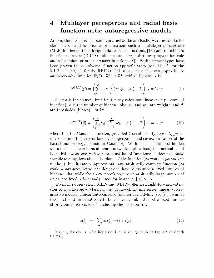
Among the most wide�spread neural networks are feedforward networks forclassi�cation and function approximation� such as multilayer perceptrons�MLP� hidden units with sigmoidal transfer functions� ���� and radial basisfunction networks �RBFN� hidden units using a distance propagation ruleand a Gaussian� or other� transfer functions� ���� Both network types havebeen proven to be universal function approximators �see ��� ��� for theMLP� and ��� ��� for the RBFN�� This means that they can approximateany reasonable function F��p� Rn �Rm arbitrarily closely by

FMLP ��p�

�� kXj��

vjl��nXi��

wijpi � �j�� �l

�A � l ���m ���

� where � is the sigmoid function �or any other non�linear� non�polynomialfunction�� k is the number of hidden units� vjl and wij are weights� and �iare thresholds �biases� � or by

FRBF ��p�

�� kXj��

vjl��nXi��

�wij � pi���� �l

�A � l ���m ����

where � is the Gaussian function� provided k is su ciently large� Approxi�mation of non�linearity is done by a superposition of several instances of thebasis function �e�g�� sigmoid or Gaussian�� With a �xed number of hiddenunits �as is the case in most neural network applications� the method couldbe called a semi�parametric approximation of functions It does not makespeci�c assumptions about the shape of the function �as would a parametricmethod�� but it cannot approximate any arbitrarily complex function �ascould a non�parametric techniqu� note that we assumed a �xed number ofhidden units� while the above proofs require an arbitrarily large number ofunits� not �xed beforehand� � see� for instance� ��� or ���From this observation� MLPs and RBFNs o�er a straight�forward exten�

sion to a wide�spread classical way of modeling time series linear autore�gressive models� Linear autoregresive time series modeling �see ��� assumesthe function F in equation � to be a linear combination of a �xed numberof previous series vectors�� Including the noise term ��

x�t� pXi��

�ix�t� i� � ��t� ����

�for simpli�cation� a univariate series is assumed� by replacing the vectors �x with

scalars x

FL�x�t� ��� � � � � x�t� p�� � ��t� ����

If p previous sequence elements are taken� one speaks of an AR p� modelof the time series �autoregressive model of order p�� Finding an appro�priate AR p� model means choosing an appropriate p and estimating thecoe cients �i� e�g� through a least squares optimization procedure �see ��for an extensive treatment of this topic�� This technique� although ratherpowerful� is naturally limited� since it assumes a linear relationship amongsequence elements� Most importantly� it also assumes stationarity of thetime series� meaning that the main moments �mean� standard deviation� donot change over time �i�e� mean and standard deviation over a part of theseries are independent of where in the series this part is extracted��It becomes clear from equations � and �� �or �� and ��� respectively�

that an MLP or RBFN can replace the linear function FL in equation �� byan arbitrary non�linear function FNN �with NN being eitherMLP or RBF�

x�t� FNN�x�t�� � � � � x�t� p�� � ��t� ����

This non�linear function can be estimated based on samples from the series�using one of the well�known learning or optimization techniques for thesenetworks �e�g� backpropagation� conjugent gradient� etc��� Making FNN

dependent on p previous sequence elements is identical to using p inputunits being fed with p adjacent sequence elements �see Fig� ��� This inputis usually refered to as a time window �see section ��� since it provides alimited view on part of the series� It can also be viewed as a simple way oftransforming the temporal dimension into another spatial dimension�Non�linear autoregressive models are potentially more powerful than lin�

ear ones in that

� they can model much more complex underlying characteristics of theseries

� they theoretically do not have to assume stationarity

However� as in static pattern recognition� they require much more care andcaution than linear methods in that they

� require large numbers of sample data� due to their large number ofdegrees�of�freedom

� can run into a variety of problems� such as over�tting� sub�optimalminima as a result of estimation �learning�� etc�� which are more severethan in the linear case �where over�tting can come about by chossingtoo high a value for the parameter p� for instance�

�����

�����

x^(t)

x(t � p)x(t � 3)x(t � 2)x(t � 1)

FNN(x(t � 1), ...)

Figure � A feedforward neural net with time window as a non�linear ARmodel

� do not necessarily include the linear case in a trivial way

Especially the �rst point is important for many real�world applicationswhere only limited data is available� A linear model might still be preferablein many cases� even if the dependencies are non�linear� The second pointconcerns the learning algorithm employed� Backpropagation very often isnot the most appropriate choice to obtain optimal models�Examples of feedforward neural networks in forecasting are �� ��� ��� ���

and numerous other papers in ��� and �����

��� Time�delay neural networks

Another mechanism to supply neural networks with �memory� to deal withthe temporal dimension is the introduction of time delays on connections�In other words� through delays� inputs arrive at hidden units at di�erentpoints in time� thus being �stored� long enough to in�uence subsequent in�puts� This approach� called a time�delay neural network �TDNN� has beenextensively employed in speech recognition� for instance� by ���� Formally�time delays are identical to time windows and can thus be viewed as au�toregressive models� as well� An interesting extension is the introduction oftime delays also on connections between hidden and output units� providingadditional� more �abstract� memory to the network�

� �Jordan� nets� moving average models

An alternative approach to modeling time series is to assume the series beinggenerated through a linear combination of q �noise� signals �see� again� ���

�This� again� is one example of a proceedings series� resulting from the annual con�

ference �Neural Networks and the Capital Markets�� providing an excellent overview of

work on forecasting with neural networks in the �nancial domain�

x�t� �

qXi��

i��t� i� � ��t� ����

FL���t� ��� � � � � ��t� q�� � ��t� ����

This is refered to as a moving average �or MA q�� model ��of order q��� Theapproach seems paradoxical at �rst a non�random time series is modeledas the linear combination of random signals� However� when viewing thelinear combination as a discrete �lter of the noise signal� the MA q� modelcan be viewed as thus A noise process usually has a frequency spectrumcontaining all or a large number of frequencies ��white� noise�� A �lter �like the MA q� model � can thus cut out any desired frequency spectrum�within the bounds of linearity�� leading to a speci�c� non�random timeseries�A combination of AR and MA components is given in the so�called

ARMA p�q� model

x�t� pXi��

�ix�t� i��qX

i��

i��t� i� � ��t� ����

FL�x�t� ��� � � � � x�t� p�� ��t� ��� � � � � ��t� q�� � ��t� ����

MA q� and ARMA p�q� models� like AR p� models� are again rather limitedgiven their linearity� and also their requirement of stationarity� Thus� anextension to the non�linear case using neural networks seems appropriatehere� as well� ��� introduce such a possibility� The most important questionto answer is this What values of �i should be taken! A common approachin MA modeling is to use the di�erence between actual and estimated �fore�cast� value as an estimate of the noise term at time t� This is justi�ed bythe following observation� Assume that the model is already near�optimal interms of forecasting� Then the di�erence between forecast and actual valuewill be close to the residual error � the noise term in equation �� Thus� thisdi�erence can be used as an estimate �� for the noise term � in equation ���

���t� x�t�� �x�t� ����

Figure � depicts a neural network realizing this assumption for the univari�ate case ���� The output of the network� which is identical to the estimateof �x�t� ��� is fed back to an additional input layer� each unit of which alsoreceives a negative version of the corresponding actual value x�t��� �avail�able at the subsequent time step� to form the desired di�erence� If a timewindow �or time delay at the input layer� is introduced� as well� the networkforms an arbitrarily non�linear ARMA p�q� model of the time series

x^(t)

x(t � 1)

x^(t � 1)–

FNN(x(t � 1), ...)

copy

Figure � A neural network with output layer feedback� realizing a non�linear ARMA model�

x�t� FNN�x�t� ��� � � � � x�t� p�� ���t� ��� � � � � ���t� q�� � ��t� ����

Simliar observations as with respect to the non�linear AR p� model in section�� must be made� As a non�linear model� the network is potentially morepowerful than traditional ARMA models� However� this must again beconsidered with care� due to the large numbers of degrees�of�freedom andthe potential limitations of the learning algorithms� A further complicationcomes from the fact that at the beginning of the sequence� no estimates �xare available� One possible way to overcome this problem is to start with �values and update the network until su cient estimates are computed� Thisrequires a certain number of cycles before the learning algorithm can beapplied� �wasting� a number of sequence elements which cannot be used fortraining� This is especially important when one wants to randomize learningby always choosing an arbitrary window from the time series� instead ofstepping thorugh the series sequentially�The network in �gure � can be considered a special case of the recurrent

network type in �gure �� usually called Jordan network after ���� It consistsof a multilayer perceptron with one hidden layer and a feedback loop fromthe output layer to an additional input �or context� layer� In addition� ���introduced self�recurrent loops on each unit in the context layer� i�e� eachunit in the context layer is connected with itself� with a weight vi smallerthan �� Without such self�recurrent loops� the network forms a non�linearfunction of p past sequence elements and q past estimates

�x�t� FNN�x�t� ��� � � � � x�t� p�� �x�t� ��� � � � � �x�t� q�� ����

The non�linear ARMA p�q� model discussed above can be said to be implic�itly contained in this network by reformulating equation �� �with the helpof equation � and �p �x�t� ��� � � � � x�t� p�� �x�t� ��� � � � � �x�t� q�� as

copy

Figure � The �Jordan� network�

�x�t� kX

j��

vjl��pXi��

�wij �x�t� i�� �x�t� i��� �z ����t�i�

��wi�p�j � wij��x�t� i�� �j�� �l

FNN�x�t� ��� � � � � x�t� p�� ���t� ��� � � � � ���t� q�� ����

l � ����

provided� p q �a similar derivation can be made for q p�� However�conventional learning algorithms for MLPs cannot trivially recogize di�er�ences between input values �in terms of them being the relevant invariances��Therefore� the explicit calculation of the di�erences in �gure � can be viewedas the inclusion of essential pre�knowledge and thus the above network seemsto be more well�suited for the implementation of a clean non�linear ARMAmodel� Nevertheless� the Jordan network can also be used for time seriesprocessing� extending the ARMA family of models by one realizing a func�tional dependency between sequence elements and estimates one one hand�and the to�be�forecast value on the other� Examples of applications with�Jordan� networks are ��� ����The self�recurrent loops in the Jordan network are another deviation of

the standard ARMA�type of models� With their help� past estimates aresuperimposed onto each other in the following way

aCi �t� f�aCi �t� �� � vi�xi�t� ��� ����

where f is the activation function� typically a sigmoid� This means thatthe activations aCi of the units in the context layer are recursively com�puted based on all past estimates �x� In other words� each such activationis a function of all past estimates and thus contains information about apotentially unlimited previous history� This property has often given riseto the argument that recurrent networks can exploit information beyond alimited time window �p or q past values�� However� in practice this cannotreally be exploited� If vi is close to �� the unit �if it uses a sigmoid transfer

function� quickly saturates to maximum activation� where additional inputshave little e�ect� If vi �� the in�uence of past estimates quickly goes to �through several applications of equation ��� So� in fact� context layers withself�recurrent loops are also rather limited in representing past information�In addition� �exibility in including past information is paid by the loss ofexplicitness of that information� since past estimates are accumulated intoone activation value�Another way of employing self�recurrent loops will be discussed below�

� Elman networks and state space models

Another common method for time series processing are so�called �linear�state space models ���� The assumption is that a time series can be de�scribed as a linear transformation of a time�dependent state � given througha state vector �s

�x�t� C�s�t� � ���t� ����

where C is a transformation matrix� The time�dependent state vector isusually also desribed by a linear model

�s�t� A�s�t� �� �B���t� ����

where A and B are matrices� and ���t� is a noise process� just like ���t� above�The model for the state change� in this version� is basically an ARMA ����process� The basic assumption underlying this model is the so�calledMarkovassumption� meaning that the next sequence element can be predicted bythe state a system producing a time series is in� no matter how the state wasreached� In other words� all the history of the series necessary for producinga sequence element can be expressed by one state vector� Since this vector��s� is continuous�valued� all possible state vectors form a Euclidean vectorspace in Rn� This model ��� can be viewed as a time series modeled interms of another one �related to the mapping between time series discussedin section �����If we further assume that the states are also dependent on the past

sequence vector �an assumption� which is common� for instance� in signalprocessing � see ����� and neglect the moving average term B���t�

�s�t� A�s�t� �� �D�x�t� �� ����

then we basically obtain an equation describing a recurrent neural networktype� known as Elman network �after ����� depicted in �gure �� The Elmannetwork is an MLP with an additional input layer� called the state layer�receiving as feedback a copy of the activations from the hidden layer atthe previous time step� If we use this network type for forecasting� and

copy

Figure � The �Elman� network as an instantiation of the state�space model�

equate the activation vector of the hidden layer with �s� the only di�erenceto equation �� is the fact that in an MLP a sigmoid activation function isapplied to the input of each hidden unit

�s�t� ��A�s�t� �� �D�x�t� ��� ����

where ���a� refers to the application of the sigmoid �or logistic� function�����exp��ai�� to each element ai of �a� In other words� the transformationis not linear but the application of a logistic regressor to the input vectors�This leads to a restriction of the state vectors to vectors within a unit cube�with non�linear distortions towards the edges of the cube� Note� however�that this is a very restricted non�linear transformation function and doesnot represent the general form of non�linear state space models �see below��The Elman network can be trained with any learning algorithm for

MLPs� such as backpropagation or conjugent gradient� Like the Jordan net�work� it belongs to the class of so�called simple recurrent networks �SRN� ����Even though it contains feedback connections� it is not viewed as a dynam�ical system in which activations can spread inde�nitly� Instead� activationsfor each layer are computed only once at each time step �each presentationof one sequence vector��Like above� the strong relationship to classical time series processing can

be exploited to introduce �new� learning algorithms� For instance� in ���the Kalman �lter algorithm� developed for the original state space model isapplied to general recurrent neural networks�Similar observations can be made about the Elman recurrent network as

with respect to the Jordan net Here� too� a number of time steps is neededuntil � after starting with � activations � suitable activations are availablein the state layer� before learning can begin� Standard learning algorithmslike backpropagation� although easy to apply� can cause problems or lead tonon�optimal solutions� Finally� this type of recurrent net also cannot reallydeal with an arbitrarily long history� for similar reasons as above �see� forinstance� ��� cited in ��� or ����� Examples of applications with �Elman�networks are ��� ��� ����

copyMLP or RBFN

MLP or RBFN

Figure � An extension of the �Elman� network as realization of a non�linearstate�space model

As hinted upon above� a general non�linear version of the state spacemodel is conceivable� as well� By replacing the linear transformation inequations �� and �� by an arbitrary non�linear function� one obtains

�x�t� F���s�t�� � ���t� ����

�s�t� F���s�t� ��� � ���t� ����

Like in the previous sections on non�linear ARMA models� these non�linearfunctions F� and F� could be modeled by an MLP or RBFN� as well� Theresulting network is depicted in �gure �� An example of the application ofsuch a network is ����

��� Multi�recurrent networks

���� and ���� has given an extensive overview of additional types of recur�rencies� time�windows and time delays in neural networks� By combiningseveral types of feedback and delay one obtains the general multirecurrentnetwork �MRN�� depicted in �gure �� First� feedback from hidden and out�put layers are permitted� From the discussions in sections �� � and � itbecomes clear that his can be viewed as a state space model� where thestate transition is modeled as a kind of ARMA ���� process� reintroducingthe B���t� term in equation ��� This view is not entirely correct� though�

Using the estimates ��x as additional inputs implicitly introduces estimatesfor the noise process ��t� in equation ��� and not for ��t� in equation ���Secondly� all input layers �the actual input� the state and the context

layer� are permitted to be extended by time�delays� such as to introduce timewindows over past instances of the corresponding vectors� This essentiallymeans that the involved processes are AR p� and ARMA p�q�� respectively�with p and q larger than ��

Output Layer

Hidden Layer

Input Layer

Context Layer

1

2

3

4In- and Output

Forward Propagation

Layer Copy

5

2

Figure � The multi�recurrent network from Ulbricht �������

Thirdly� like in the Jordan network� self�recurrent loops in the statelayer can be introduced� The weights of these loops� and the weights ofthe feedback copies resulting from the recurrent one�to�one connections�are chosen such as to scale the theoretically maximum input to each unitin the state layer to �� and to give more or less weight to the feedbackconnections or self�recurrent loops� respectively� If� for instance� �� " ofthe total activation of a unit in the state layer comes from the hidden layerfeedback� and �� " comes from self�recurrency� the state vector will tendto change considerably at each time step� If� on the other hand� only ��" come from the hidden layer feedback� and �� " from the self�recurrentloops the state vector will tend to remain similar to the one at the previoustime step� ��� speaks of �exible and sluggish state spaces� respectively� Byintroducing several state layers with di�erent such weighting schemes� thenetwork can exploit both the information of rather recent time steps and akind of average of several past time steps� i�e� a longer� averaged history�It is clear that a full��etched version of the MRN contains a very large

number of degrees�of�freedom �weights� and requires even more care thanthe other models discussed above� Several empirical studies ��� ��� haveshown� however� that for real�world applications� some versions of the MRNcan signi�cantly outperform most other� more simple� forecasting methods�The actual choice of feedback� delays and weightings still depends largelyon empirical evaluations� but similar iterative estimation algorithms as weresuggested by �� �for obtaining appropriate parameter values for ARMAmodels� appear applicable here� too�Another advantage of self�recurrent loops becomes evident in applica�

tions where patterns in the time series can vary in time scale� This phe�nomenon is called time warping� and is especially known in speech recog�nition� where di�erent speech patterns can vary in length and relationshipsbetween segments dependent on speaking speed and intonation ���� In au�toregressive models with �xed time windows� such distorted patterns leadto vectors that do not share su cient similarities to be classi�ed correctly�This is sometimes called the temporal invariance problem � the problem of

Figure � A simple network with a time�dependent weight matrix� producedby a second neural net�

recognizing temporal patterns independent of their duration and temporaldistortion� In a state space model� implemeted as a recurrent network withself�recurrent loops such invariances can be dealt with� especially when slug�gish state spaces are employed� If states in the state space model are forcedto be similar at subsequent time steps� events can be treated equally �orsimilarly� even when the are shifted along the temporal dimension� Thisproperty is discussed extensively in ����

Neural nets producing weight matrices�

timedependent state transitions

The original state space model approach �equations �� and ��� left openthe possibility of making all matrices A through C time�dependent as well�This allows for the modeling of non�stationary time series and series wherethe variance of the noise process changes over time� In neural network termsthis would mean the introduction of time�varying weight matrices� ��� introduced a small neural network model that can be viewed in the

context of time�dependent transition matrices� It consist of two feedforwardnetworks � one mapping an input sequence onto an output� and another oneproducing the weight matrix for the �rst network ��gure ��� Even thoughnot a state�space model but rather a AR �� model of the input sequence�it realizes a mapping with a variable matrix �the weight matrix of the �rstnetwork�� This network was used to learn formal languages� such as parityor others� A similar example can be found in ����In this context� other approaches to inducing �nite�state automata into

neural networks should be mentioned �e�g� ����� A �nite state automatonis another classical model to describe time series� although on a more ab�stract level � the level of categories instead of continuous�valued input� If acategorization process is assumed before the model is applied it can also beused for time series as the ones discussed above� An automaton is de�nedas a set of states �discrete and �nite� so there is no concept of state space

�By �time�varying� I mean varying on the time�scale of the series� Weight changes due

to learning are not considered here�

a

b

a

b

a,b

Figure �� A �nite state automaton for modeling time series

in this model� with arcs between them corresponding to state transitionstaken dependent on the input� For instance� in �gure ��� if � starting fromthe left�most state �node� � an #a� is encountered� the automaton wouldjump to state �� while if a #b� is encountered� it would remain in state ��Depending on what types of arcs emanate from a state� a prediction canbe made with respect to what input element must follow� provided thatthe input is �grammatical�� i�e� corresponds to the grammar the automatonimplements� This is especially useful for sequences in speech or language� ��� have shown that a neural network can be set or trained such as

to implement such an automaton� While this concept cannot directly beapplied to real�world sequences like the ones above� it points to anotheruseful application of neural networks� especially when going from �nite�discrete states to continuous state spaces� This is exactly what an Elmannetwork or the model by ��� realizes�

� Other topics

The story does not end here� There are many more important topics con�cerning time series processing and the use of neural networks in this �eld�Some topics that could not be covered here� but are of equal importance asthe ones that were� are the following�

� many time series applications are tackled with fully recurrent net�works� or networks with recurrent architectures di�erent from the onesdiscussed �e�g� ����� Special learning algorithms for arbitrary recur�rent networks have been devised� such as backpropagation in time ���and real�time recurrent learning �RTRL� ����

� many authors use a combination of neural networks with so�calledhidden Markov models �HMM� for time series and signal processing�HMMs are related to �nite automata and describe probabilities forchanging from one state to the other� See� for instance� �� or thetreatment in ���

� unsupervised neural network learning algorithms� such as the self�organizing feature map� can also be applied in time series processing�both in forecasting �� and classi�cation ���� The latter applicationconstitutes an instance of so�called spatio�temporal clustering� i�e� theunsupervised classi�cation of time series into clusters � in this casethe clustering of sleep�EEG into sleep stages�

� a number of authors have investigated the properties of neural net�works viewed as dynamical systems� including chaotic attractor dy�namics� Examples are ��� and ����

The focus of this paper was to introduce the most widely used architecturesand their close relationships to more classical approaches to time seriesprocessing� The approaches presented herein can be viewed as startingpoints for future research� since the potential of neural networks � especiallywith respect to dynamical systems � is by far not fully exploited yet�

� Conclusion

As mentioned initially� this overview of neural networks for time series pro�cessing could only scratch the surface of a very lively and important �eld�The paper has attempted to introduce most of the basics of this domain�and to stress the relationship between neural networks and more tradi�tional statistical methodologies� It underlined one important contributionof neural networks � namely their elegant ability to approximate arbitrarynon�linear functions� This property is of high value in time series processingand promises more powerful applications� especially in the sub�eld of fore�casting� in the near future� However� it was also emphasized that non�linearmodels are not without problems� both with respect to their requirementfor large data bases and careful evaluation and with respect to limitationsof learning or estimation algorithms� Here� the relationship between neuralnetworks and traditional statistics will be essential� if the former is to liveup to the promises that are visible today�

Acknowledgments

The Austrian Research Institute for Arti�cial Intelligence is supported bythe Austrian Federal Ministry of Science� Research� and the Arts� I partic�ularly thank Claudia Ulbricht� Adrian Trapletti and the research group ofProf� Manfred Fischer� the cooperation with which has been the basis forthis work� for valuable comments on this manuscript�

References

��� Baumann T�� Germond A�J�� Application of the Kohonen Network to Short�Term Load Forecasting� in Proc� PSCC� Avignon� Aug �� � Sep �� ���

�� Bengio Y�� Simard P�� Frasconi P�� Learning long�term dependencies withgradient descent is di�cult� IEEE Trans� Neural Networks ����� �� ��������

��� Bengio Y�� Neural Networks for Speech and Sequence Recognition� Thomson�London� ���

��� Bera A�K�� Higgins M�L�� ARCH models� properties� estimation and testing�Journal of Economic Surveys ����� �� ����� ���

��� Bishop C�� Neural Networks for Pattern Recognition� Clarendon Press� Ox�ford� ���

��� Bourlard H�� Morgan N�� Merging Multilayer Perceptrons and HiddenMarkov Models� Some Experiments in Continuous Speech Recognition� Int�Computer Science Institute �ICSI�� Berkeley� CA� TR������ ���

� � Box G�E�� Jenkins G�M�� Time Series Analysis� Holden�Day� San Francisco�� ��

��� Broomhead D�S�� Lowe D�� Multivariable Functional Interpolation andAdaptive Networks� Complex Systems ��������� ����

�� Chakraborty K�� Mehrotra K�� Mohan C�K�� Ranka S�� Forecasting the Be�havior of Multivariate Time Series Using Neural Networks� Neural Networks����� ��� �� ��

���� Chappelier J��C�� Grumbach A�� Time in Neural Networks� in SIGART BUL�LETIN� ACM Press ����� ���

���� Chat�eld C�� The Analysis of Time Series � An Introduction� Chapman andHall� London� �th edition� ���

��� Connor J�� Atlas L�E�� Martin D�R�� Recurrent Networks and NARMA Mod�eling� in Moody J�E�� et al��eds��� Neural Information Processing Systems ��Morgan Kaufmann� San Mateo� CA� pp��������� ��

���� Cottrell G�W�� Munro P�W�� Principal components analysis of images viabackpropagation� Proc�Soc�of Photo�Optical Instr� Eng�� ����

���� Cybenko G�� Approximation by Superpositions of a Sigmoidal Function�Math Control Signals Syst� ���������� ���

���� Debar H�� Dorizzi B�� An Application of a Recurrent Network to an Intru�sion Detection System� in IJCNN International Joint Conference on NeuralNetworks� Baltimore� IEEE� pp�� ������ ��

���� DeCruyenaere J�P�� Hafez H�M�� A Comparison Between Kalman Filtersand Recurrent Neural Networks� in IJCNN International Joint Conferenceon Neural Networks� Baltimore� IEEE� pp�� ���� ��

�� � Dor�ner G�� Leitgeb E�� Koller H�� Toward Improving Exercise ECG forDetecting Ischemic Heart Disease with Recurrent and FeedForward NeuralNets� in Vlontzos J�� et al��eds��� Neural Networks for Signal Processing IV�IEEE� New York� pp� ������ ���

���� Duda R�O�� Hart P�E�� Pattern Classi�cation and Scene Analysis� John Wi�ley � Sons� N�Y�� � ��

��� Elman J�L�� Finding Structure in Time� Cognitive Science ������ � ������

��� Giles C�L�� Miller C�B�� Chen D�� Chen H�H�� Sun G�Z�� Lee Y�C�� Learningand Extracting Finite State Automata with Second�Order Recurrent NeuralNetworks� Neural Computation ����� ������� ��

��� Gordon A�� Steele J�P�H�� Rossmiller K�� Predicting Trajectories Using Re�current Neural Networks� in Dagli C�H�� et al��eds��� Intelligent Engineer�ing Systems through Arti�cial Neural Networks� ASME Press� New York�pp������ �� ���

�� Girosi F�� Poggio T�� Networks and the Best Approximation Property� Bio�logical Cybernetics ������� �� ���

��� Hertz J�A�� Palmer R�G�� Krogh A�S�� Introduction to the Theory of NeuralComputation� Addison�Wesley� Redwood City� CA� ���

��� Ho T�T�� Ho S�T�� Bialasiewicz J�T�� Wall E�T�� Stochastic Neural Adap�tive Control Using State Space Innovations Model� in International JointConference on Neural Networks� IEEE� pp��������� ���

��� Hornik K�� Stinchcombe M�� White H�� Multi�layer Feedforward Networksare Universal Approximators� Neural Networks �� ������� ���

��� Jordan M�I�� Serial Order� A Parallel Distributed Processing Approach�ICS� UCSD� Report No� ����� ����

� � Kamijo K�� Tanigawa T�� Stock Price Pattern Recognition� A RecurrentNeural Network Approach� in Trippi R�R� � Turban E��eds��� Neural Net�works in Finance and Investing� Probus� Chicago� pp��� �� �� ���

��� Kolen J�F�� Exploring the Computational Capabilities of Recurrent NeuralNetworks� Ohio State University� ���

�� Kolen J�F�� Pollack J�B�� The Observers� Paradox� Apparent ComputationalComplexity in Physical Systems� Journal of Exp� and Theoret� Arti�cialIntelligence ����� ���

���� Kurkova V�� Universal Approximation Using Feedforward Neural Networkswith Gaussian Bar Units� in Neumann B��ed��� Proceedings of the TenthEuropean Conference on Arti�cial Intelligence �ECAI��� Wiley� Chichester�UK� pp���� � � ��

���� Lee C�H�� Park K�C�� Prediction of Monthly Transition of the CompositionStock Price Index Using Recurrent Back�propagation� in Aleksander I� �Taylor J��eds��� Arti�cial Neural Networks �� North�Holland� Amsterdam�pp���� ���� ��

��� Morgan D�P�� Sco�eld C�L�� Neural Networks and Speech Processing� KluwerAcademic Publishers� Boston� ���

���� Mozer M�C�� Neural Net Architectures for Temporal Sequence Processing�Predicting the Future and Understanding the Past� in A� Weigend and N�Gershenfeld �Eds��� Time Series Prediction Forecasting the Future and Un�derstanding the Past� Addison�Wesley Publishing� Redwood City� CA� ���

���� Pollack J�B�� The Induction of Dynamical Recognizers� Machine Learning������ ��� ���

���� Port R�F�� Cummins F�� McAuley J�D�� Naive time� temporal patterns� andhuman audition� in Port R�F�� van Gelder T� �eds��� Mind as Motion� MITPress� Cambridge� MA� ���

���� Refenes A�N�� Azema�Barac M�� Chen L�� Karoussos S�A�� Currency ex�change rate predicition and neural network design strategies� Neural Com�puting and Applications ����� ���

�� � Refenes A�N��ed��� Neural Networks in the Capital Markets� Proceedings ofthe �rst International Workshop on Neural Networks in the Capital Markets�London� Nov ����� ���

���� Refenes A�N�� Zapranis A�� Francis G�� Stock Performance Modeling UsingNeural Networks� A Comparative Study with Regression Models� NeuralNetworks ����� � ������ ���

��� Rementeria S�� Oyanguren J�� Marijuan G�� Electricity Demand Predic�tion Using Discrete�Time Fully Recurrent Neural Networks� Proceedings ofWCNN���� CA� USA� ���

���� Roberts S�� Tarassenko L�� The Analysis of the Sleep EEG using a Multi�layer Neural Network with Spatial Organisation� IEE proceedings Part F���� ������ ��

���� Rohwer R�� The Time Dimension of Neural Network Models� SIGART BUL�LETIN� ACM Press ������ ���

��� Rumelhart D�E�� Hinton G�E�� Williams R�J�� Learning Internal Representa�tions by Error Propagation� in Rumelhart D�E� � McClelland J�L�� ParallelDistributed Processing� Explorations in the Microstructure of Cognition� Vol�� Foundations� MIT Press� Cambridge� MA� ����

���� Schmidhuber J�� A Local Learning Algorithm for Dynamic Feedforward andRecurrent Networks� Connection Science ����� ������� ���

���� Trippi R�R�� Turban E��eds��� Neural Networks in Finance and Investing�Probus� Chicago� ���

���� Ulbricht C�� Dor�ner G�� Canu S�� Guillemyn D�� Marijuan G�� Olarte J��Rodriguez C�� Martin I�� Mechanisms for Handling Sequences with Neu�ral Networks� in Dagli C�H�� et al��eds��� Intelligent Engineering Systemsthrough Arti�cial Neural Networks� Vol� � ASME Press� New York� ��

���� Ulbricht C�� Multi�Recurrent Networks for Tra�c Forecasting� in Proceed�ings of the Twelfth National Conference on Arti�cial Intelligence� AAAIPress�MIT Press� Cambridge� MA� pp��������� ���

�� � Ulbricht C�� State Formation in Neural Networks for Handling TemporalInformation� Institut fuer Med�Kybernetik u� AI� Univ� Vienna� Dissertation����

���� Ulbricht C�� Dor�ner G�� Lee A�� Forecasting fetal heartbeats with neu�ral networks� to appear in� Proceedings of the Engineering Applications ofNeural Networks �EANN� Conference� ���

��� Weigend A�S�� Rumelhart D�E�� Huberman B�A�� Back�Propagation�Weight� Elimination and Time Series Prediction� in Touretzky D�S�� etal��eds��� Connectionist Models� Morgan Kaufmann� San Mateo� CA� pp��������� ���

���� Weigend A�S�� Gershenfeld N�A� �eds��� Time Series Prediction Forecastingthe Future and Understanding the Past� Reading� MA� Addison Wesley� ���

���� Vlontzos J�� Jenq�Neng H�� Wilson E��eds��� Neural Networks for SignalProcessing IV� IEEE� New York� ���

��� Waibel A�� Consonant Recognition by Modular Construction of LargePhonemic Time�delay Neural Networks� in Touretzky D��ed��� Advances inNeural Information Processing Systems� Morgan Kaufmann� Los Altos� CA�pp������ ���

���� White H�� Economic Prediction Using Neural Networks� The Case of IBMDaily Stock Returns� in Trippi R�R� � Turban E��eds��� Neural Networks inFinance and Investing� Probus� Chicago� pp�������� ���

���� Widrow B�� Stearns S�D�� Adaptive Signal Processing� Prentice�Hall� Engle�wood Cli�s� NJ� ����

���� Williams R�J�� Zipser D�� Experimental Analysis of the Real�time RecurrentLearning Algorithm� Connection Science ����� � ����� ���

���� Williams R�J�� Training Recurrent Networks Using the Extended KalmanFilter� in International Joint Conference on Neural Networks� Baltimore�IEEE� pp������� ��