Embed Size (px)
Citation preview
Design of Large Scale Transportation Service
Networks with Consolidation: Models,
Algorithms and Applications
by
Niranjan Krishnan
Submitted to the Department of Civil and EnvironmentalEngineering
in partial fulfillment of the requirements for the degrees of
Master of Science in Operations Research
and
Master of Science in Transportation
at the
MASSACHUSETTS INSTITUTE OF TECHNOLOGY
February 1998
@ Massachusetts Institute of Technology 1998. All rights reserved.
A uthor .............. .... ...... . .........................Department of Civil and Environmental Engineering
Jan 9, 1998
Certified by......:...... ..........................................Cynthia Barnhart
Associate Professor. Thesis Supervisor
Accepted by.........Joseph M. Sussman
Chairman, Departrmental Committee on Graduate Students
Accepted by ...................Robert M. Freund
Codirector, Operations Research Center

Design of Large Scale Transportation Service Networks
with Consolidation: Models, Algorithms and Applications
by
Niranjan Krishnan
Submitted to the Department of Civil and Environmental Engineeringon Jan 9, 1998, in partial fulfillment of the
requirements for the degrees ofMaster of Science in Operations Research
andMaster of Science in Transportation
Abstract
The primary focus of our research has been to develop models and algorithms tooptimize large scale service network design problems for transportation providers.Service network design problems arise at airlines (passenger and cargo), truckingcompanies, railroads, etc., wherever there is a need to determine cost minimizingroutes and schedules, given constraints on resource availability and level of service.We have developed models and a novel decomposition technique to solve large scaleservice network design problems with time windows and demand consolidation. Weapply our models and algorithms to design the service network of a key player in theexpress shipment delivery industry. Our approach results in savings in total operatingcosts and provides a valuable tool for making decisions at strategic and tactical levels.
Thesis Supervisor: Cynthia BarnhartTitle: Associate Professor

Biographical Note
Niranjan Krishnan (b.1973)
Niranjan Krishnan joined Indian Institute of Technology - Madras, in 1991 to
study Civil Engineering. He graduated from the Institute's undergraduate program
with top honors in 1995. The basic focus of Krishnan's work at MIT has been on
applying OR/MS techniques for modeling transportation and logistics systems. At
MIT, Krishnan worked as the Teaching Assistant to a core graduate course in Trans-
portation Systems Analysis in the Fall of 1997. Krishnan's primary research interests
include network algorithms, large scale optimization techniques, transportation and
logistics analysis, and Wodehousian analysis of aristocracy in Edwardian England.
Acknowledgments
Firstly, I am pleased to have this opportunity to thank Prof. Cynthia Barnhart forbeing a wonderful research advisor and a good friend. I am amazed by Cindy's enthu-siasm for research and her patience with students. I thank in particular, her effortsin improving the clarity of the thesis.
I am obliged to Dr. Keith Ware and Mr. Greg Reinhardt of UPS Airlines for theirhelp throughout. I appreciate all the administrative help from Lisa Bleheen, MariaMarangiello, Sydney Miller, Cindy Stewart and Paulette Mosley. Many thanks to thefaculty and students of CTS for an excellent experience and to Prof. Joseph Sussmanfor his inimitable style of teaching 1.201, which was such a unique course for me.
It is a privilege to express my gratitude towards IIT Madras, my alma mater, forthe training and the intangible qualities I acquired, and most of all, for the four mem-orable years. I am extremely thankful to Prof. P. Srinivasa Rao, my undergraduateadvisor and guru, for all his help, advice and inspiration.
A special word of appreciation for my friends and fellow occupants of 5-012: DaekiKim, for his insights and help especially in the form of code, Francisco Jauffred, thewizard of project workstations, Hong Jin, for useful exchange of ideas, and AndyArmacost, for his unbridled enthusiasm on the project. I acknowledge the veteranIIT-Mafia (sic) in CTS, Shenoi, Sudhir, Ashok and not to mention Hari, for alwayslending an ear.
I am grateful to my buddies who, knowingly or unknowingly, have helped me inso many ways:
Kishore, the crown-prince of Vizag, for those discussions on everything under thesun, Rajagopal, especially for being a such a fine fellow and allowing unrestrictedapplication of his automotive assets, Sivakumar, for his lively narratives, Gautam,for re-creating those A-3 days back again, and Anil, for the sponsored dinners andhis clearly biased, nevertheless amusing, diatribe on Azhar.
Anand, Mukundan, Jennifer, and members of aloo-gobi fan club, Sanjay and Pay-man, for being terrific friends.
O.P.Agarwal, the politician's antidote to Humphrey Appleby, especially for hisIIT-M tales of yore, over cups of coffee.
Venkat, Partees: Chandra, Subbu and Sreeram, and Mathew, for all the fun atMIT.
Handy, Narada, Mux, Money Order, Casual, Mama, PG, Gopal, Ben, PK, RMS,Rugby, and Ramki for the much needed dose of insanity and sanity (sometimes) fromtime to time.
I do not find enough words when I want to thank my mother and brothers,Prasanna, Ravi, Sashi and Karthi, for everything.
Dedication
To the memory of two people whose company I will miss for eternity:
My father, for more reasons than I could possible accomodate on a thesis
and,
Annu, my mentor, whom I could always turn to.
Contents
1 Introduction
1.1 Network Design Problem . . . . . . . . . . . . . . . . .
1.1.1 Baseline Network Design Problem Formulation.
1.1.2 Literature . . . . . . . . . . . . . . . . . . . . .
1.2 Contributions ..... ... .. ... ... .. .. .. .
1.3 Outline of the Thesis ...................
2 Transportation Service Network Design
2.1 Problem Description ...................
2.2 Service Network Design Problem Formulations . . . . .
2.2.1 Node-Arc Formulation ..............
2.2.2 Path Formulation .................
2.2.3 Tree Formulation .................
2.2.4 Comparison of Formulations . . . . . . . . . . .
2.3 Literature . . . . . . . . . . . . . . . . . . . . . . . . .
2.4 Decomposition Solution Approach . . . . . . . . . . . .
2.4.1 Decomposition Algorithm . . . . . . . . . . . .
2.4.2 Shipment Flow Model Description . . . . . . . .
3 Routing for Transportation Service Network Design:
Solutions
3.1 Valid Inequalities ......................
3.1.1 Chvatal-Gomory Cuts ...............
Models and
34
... ... . 34
... ... . 35
12
. . . . . . . . 12
. . . . . . . . 13
. .... ... 14
. .... ... 16
.. ... ... 18
20
... ... .. 20
. . . . . . . . 21
... ... .. 21
... ... .. 22
... ... .. 24
. . . . . . . . 25
... ... .. 26
. . . . . . . . 29
. . . . . . . . 30
. . . . . . . . 31

3.1.2 Cutset Inequalities .................
3.2 The Approximate Service Network Design Cutset Model
3.2.1 Approximate SNDP Formulations . . . . . . . . .
3.3 Literature . . . . . . . . . . . . . . . . . . . . . . . . . .
3.4 Solution Approach .....................
3.4.1 LP solution . . . . . . . . . . . . . . . . . . . . .
3.4.2 IP solution . . . . . . . . . . . . . . . . . . . . . .
. ..... . 35
. . . . . . . 36
. . . . . . . 37
. ..... . 38
.. .... . 38
.. .... . 38
.. .... . 40
4 Shipment Flow Problem: Models and Applications 44
4.1 Baseline Multicommodity Flow Problem Formulation . ........ 44
4.2 Applications of Multicommodity Flow Models . ............ 45
4.2.1 Transportation and Logistics . .................. 45
4.2.2 Other Applications ...................... .. 47
4.3 Multicommodity Flow Solution Techniques . .............. 48
4.4 Integer Multicommodity Flow Problems . ............... 50
4.4.1 Integer MCF Applications .................... 50
4.4.2 Integer MCF Solution Techniques . ............... 50
4.5 Location Elimination Model (LEM) . ............... . . . 51
4.5.1 LEM Path Formulation. . .................. .. 52
4.5.2 LEM Tree Formulation ................... ... 54
4.6 LEM LP Relaxation Solution ...................... 55
4.6.1 Solution to the Path Formulation LP . ............. 55
4.6.2 Solution to the Tree Formulation LP . ............. 56
4.7 LEM IP Solution ............................. 57
5 Service Network Design for Express Shipment Delivery: A Case
Study 58
5.1 Express Shipment Delivery Operation . ................. 58
5.1.1 Problem Description ....................... 59
5.1.2 The Planning Process ...................... 60
5.2 Express Shipment Service Network Design . .............. 62

5.2.1 Design Variables ......................... 62
5.2.2 Side Constraints ......................... 63
5.3 Routing Model for Express Shipment Delivery . ............ 65
5.3.1 Cutset Inequalities ................ ........ 66
5.3.2 ESSNDP-Approx Model ................ ..... 66
5.3.3 ESSNDP-Approx Solution Algorithm . ............. 67
5.4 Decomposition Solution Algorithm for Express Shipment Delivery . 68
5.5 Computational Results .......................... 69
5.5.1 Data Description ........................ 69
5.5.2 R esults . . . . . . . . . . . . . . . . . . . . . . . . . . . . .. . 69
5.5.3 Scenario Analysis ......................... 75
6 Closure 82
6.1 Conclusions . . . . . . . . . . . . . . . . . . . ... . . . . . .. . . .. 82
6.2 Future Research Directions ........................ 82
A Notations 84
A .1 SE T S . . . . . . . . . . . . . . . . . . . . . . . . . . . . . . .. .. . 84
A.2 PARAMETERS .............................. 85
A.3 INDICATOR VARIABLES ....................... 85
A.4 DECISION VARIABLES ......................... 86
B Model Formulations 87
B.1 Baseline Network Design Problem Formulation . ............ 87
B.2 Service Network Design Problem Formulations . ............ 88
B.2.1 Node-Arc Formulation ...................... 88
B.2.2 Path Formulation ......................... 88
B.2.3 Tree Formulation ......................... 89
B.3 The Approximate Service Network Design Cutset Model ....... 90
B.3.1 Node-Arc Formulation ...................... 90
B.3.2 Route Formulation ........................ 90
B.4 Shipment Flow Models .......................... 91
B.4.1 Baseline Multicommodity Flow Problem Formulation .... . 91
B.4.2 Location Elimination Model Path Formulation ........ . 91
B.4.3 Location Elimination Model Tree Formulation ........ . 92
B.5 Routing Model for Express Shipment Delivery . ............ 93

List of Tables
2.1 Comparison of SNDP Formulations . . . . . . . .
5.1
5.2
5.3
5.4
5.5
5.6
5.7
5.8
5.9
5.10
5.11
5.12
Data Description (before ground consolidation)
Data Description (after ground consolidation)
R esults . . . . . . . . . . . . . . . . . . . . . . .
Analysis for DS3 .................
Cost Distribution for DS3 ............
Aircraft Arrival Pattern at the Hubs for DS3 . .
Results of Scenario Analysis . . . . . . . . . . .
Cost Distribution for Scenario 1 . . . . . . . . .
Cost Distribution for Scenario 2 . . . . . . . . .
Cost Distribution for Scenario 3 . . . . . . . . .
Cost Distribution for Scenario 4 . . . . . . . . .
Cost Distribution for Scenario 5 . . . . . . . . .
5.13 Cost Distribution for Scenario 6
. . . . . . . . . . 70
. . . . . . . . . . 70
. ..... ... . 72
. ..... ... . 72
. ..... ... . 73
. . . . . . . . . . 73
. . . . . . . . . . 80
. . . . . . . . . . 80
. . . . . . . . . . 80
. . . . . . . . . . 81
. . . . . . . . . . 81
. . . . . . . . . . 81

List of Figures
2-1 Decomposition Algorithm ........................ 32
3-1 Illustration: Synchronized Colummn and Row Generation ....... . 41
3-2 Illustration: Branch-and-Price ...................... 43
5-1 Illustration for Disproportionate Demand Distribution ......... 74
Chapter 1
Introduction
1.1 Network Design Problem
Network Design Problem requires the determination of facility locations and the rout-
ing of demand on the network of facilities such that the sum of fixed cost associated
with locating the facilities facilities and the variable cost associated with the flow of
demand is minimized. We motivate the Network Design Problem with an example of
supply chain planning (see Sheffi [82]). In a typical supply chain operation, different
raw materials from suppliers are fed into different plants, which manufacture prod-
ucts for consumption (commodities). The products from manufacturing plants are
stored in regional warehouses or distribution centers (DCs) that cater to the needs of
different customer zones. In designing such a system the questions that arise are:
* How many facilities such as suppliers for raw materials, plants and DCs are
needed, where should they be located and at which capacity should they oper-
ate?
* How much of each product from each plant should be routed through each DC
to each customer zone so that all the demand is met ?
The overall objective of such a planning exercise is to minimize total cost, that is a
sum of fixed costs and variable costs. Such a planning problem belongs to a general
class of mixed integer programming problems called the Network Design Problem
(NDP). We present below a mathematical formulation of NDP and a survey of recent
literature on this subject.
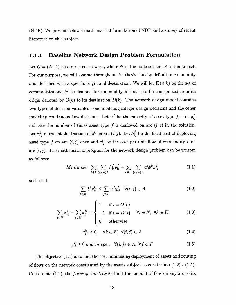
1.1.1 Baseline Network Design Problem Formulation
Let G = (N, A) be a directed network, where N is the node set and A is the arc set.
For our purpose, we will assume throughout the thesis that by default, a commodity
k is identified with a specific origin and destination. We will let K(3 k) be the set of
commodities and bk be demand for commodity k that is to be transported from its
origin denoted by O(k) to its destination D(k). The network design model contains
two types of decision variables - one modeling integer design decisions and the other
modeling continuous flow decisions. Let u1 be the capacity of asset type f. Let y:
indicate the number of times asset type f is deployed on arc (i, j) in the solution.
Let xi represent the fraction of bk on arc (i, j). Let hf be the fixed cost of deploying
asset type f on arc (i, j) once and ci be the cost per unit flow of commodity k on
arc (i, j). The mathematical program for the network design problem can be written
as follows:
Minimize Z h~y + CI .kI ,(1.1)kfEF (i,j)EA kEK (i,j)EA
such that:
bZ ufy V(i,j) E A (1.2)kEK fEF
1 if i = O(k)E xi - E zi = -1 ifi=D(k) Vi E N, Vk E K (1.3)
jEN jEN0 otherwise
xk >0, Vk E K, V(i,j) EA (1.4)
y. 2 0 and integer, V(i,j) E A, Vf E F (1.5)
The objective (1.1) is to find the cost minimizing deployment of assets and routing
of flows on the network constituted by the assets subject to constraints (1.2) - (1.5).
Constraints (1.2), the forcing constraints limit the amount of flow on any are to its
capacity, as determined by the value of design variables. Constraints (1.3) are the
flow conservation constraints that ensure that each commodity is fully serviced from
its origin to destination. Constraints (1.4) ensure non-negativity of commodity flows
and constraints (1.5) ensure the integrality and non-negativity of design variables.
1.1.2 Literature
A survey of literature on network design can be found in Minoux [66], Magnanti and
Wong [64] and Kim [52]. For a course on the design of survivable networks under
connectivity constraints in telecommunications, we refer the reader to Stoer [84]. We
outline some of the recent research in the area below:
* Magnanti et al. [63] demonstrate how to tailor Benders' decomposition to
the uncapacitated network design problem. The uncapacitated network de-
sign problem is a variant of the general network design problem where there are
no forcing constraints (1.2).
* Gendron and Crainic [38] analyze classical relaxation methods applied to several
formulations of a fixed charge multicommodity network design problem using
resource-decomposition based solution techniques.
* Clarke and Gong [24] contrast link-based and path-based formulations of the
capacitated telecommunication network design problem. They strengthen the
model using valid inequalities developed by Magnanti et al. [62] and propose
SOS constraints to take advantage of SOS branching in MINTO (the Mixed
INTeger Optimizer [69]).
* Li et al. [57] consider the computational complexity of point-to-point delivery
problems and closely related point-to-point connection problems. They prove
that all variations of both the problems are NP -hard, but there are polynomial
algorithms for special cases.
* Medhi and Tipper [65] present different solution approaches to a multi-hour
communication network design problem. They compare the approaches based
on a genetic algorithm and Lagrangean relaxation.
* Balakrishnan et al. ([5] and [6]) present models and algorithms for the multi-
level network design problem that addresses topological design trade-offs in
hierarchical networks.
* Balakrishnan et al. [8] develop and test a decomposition algorithm to gener-
ate cost-effective expansion plans with performance guarantees, for local access
networks.
* Magnanti et al. ([61] and [62]) study two core subproblems of a specialized ca-
pacitated network design problem called the Network Loading Problem (NLP).
They develop families of facets and completely characterize the convex hull of
feasible solutions to the integer programming formulation of the problems.
* Balakrishnan et al. [7] study a class of models, called overlay optimization
problems, composed of "base" and "overlay" subproblems, linked by the re-
quirement that the overlay solution be contained in the base solution. They
describe a heuristic procedure and establish worst-case performance guarantees
for the uncapacitated multicommodity network design problem.
Some of the recent developments in the area have been in approximation algorithms.
* Goemans and Williamson [40] demonstrate how the primal-dual method of solv-
ing linear programs can be modified to provide good approximation algorithms
for a wide variety of NP-hard problems. They also provide a good summary
of developments in primal-dual approximation algorithms for network design
problems.
* Agrawal, Klein and Ravi [2] introduce the use of approximation schemes for
network design problems without reference to linear programming.
* Goemans and Williamson [41] expand the approach of Agrawal, Klein and Ravi
[2] and make explicit use of linear programming to provide an approximation
scheme for network design problems.

* Williamson et al. [88] present the first polynomial-time algorithm for a class of
network design problems including the Steiner network problem (see Ahuja et
al. [3]) and the survivable network design problem (see Stoer [84] for details)
that arises in telecommunication.
* Gabow et al. [37] improve the approximation algorithm presented by Williamson
et al. [88] for the survivable network design problem.
* Goemans et al. [39] study a class of network design problems where one needs
to find a minimum cost network satisfying certain connectivity requirements
and present an approximation algorithm with a performance guarantee that is
harmonic with respect to the requirement function.
* Hochbaum and Naor [46] use the results of Goemans et al. [39] and provide an
approximation scheme for network design problems with some special connec-
tivity requirements.
The major disadvantage of approximation algorithms has been the fact that the
bounds given by approximation schemes are very loose and the analyses done to
arrive at the bounds are usually very tight. Also the treatment of approximation
algorithms in the literature has been rather theoretical in nature and there is a dearth
of computational testing on practical applications.
1.2 Contributions
The contributions of our research are three-fold:
Modeling Contributions
We have developed an iterative modeling framework for large scale transporta-
tion service network design problems with time windows. Within our frame-
work, we divide the problem into two subproblems. The first subproblem in-
volves routing decisions and the second involves shipment flow decisions. We
use an approximate service network design model for routing decisions. For

the shipment flow decisions, we have developed a novel variant of mixed integer
multicommodity flow models called the Location Elimination Model (LEM). We
present two equivalent formulations of LEM based on path-based and tree-based
definition of flow variables. LEM enables the overall framework to provide in-
sight out of an infeasible routing plan and enables decisions to be made that
subsequently increase the ease of subproblem solution future iterations. Since
the amount of memory needed is the key stumbling block, the exactness of
the modeling framework increases if the memory availability is increased or if
the problem size is reduced, thereby making apparent the trade-off between
computer memory and exactness of the solution.
Algorithmic Contributions
We have contributed a decomposition solution algorithm for service network de-
sign that is particularly amenable for large scale problems. The overall solution
algorithm involves solution of two kinds of subproblems, one for each type of
decision variable. The route generation subproblem is a large scale general inte-
ger program and is solved using a Branch-and-Price-and-Cut approach, where
both route variables and violated constraints are generated on an "as needed"
basis. We use a Branch-and-Price strategy to solve the shipment flow subprob-
lem, LEM, where the shipment flow variables are generated on an "as needed"
basis by solving a series of shortest path subproblems.
We provide a proof-of-concept of the efficacy of our solution approach by
solving the service network design problem of a large carrier in the express
shipment delivery industry. We are unable to generate optimal IP solutions due
to the huge size of the carrier's operations and NP-completeness that typifies
service network design problems. However, our solution approach provides IP
feasible solutions that result in annual cost savings measuring in tens of millions
of dollars, with run times acceptable for strategic planning.
Applied Contributions
We have developed a modeling framework and a decomposition solution ap-
proach for service network design problems that arise at airlines, trucking com-
panies, railroads, supply chains, etc. The common characteristic of these service
network design problems is the need to determine cost minimizing routes and
schedules, given constraints on resource availability and level of service. De-
pending on the specific operating characteristics of the application, additional
constraints may be necessary. For our express shipment delivery application,
we illustrate how to model fleet balance constraints, fleet size constraints, fleet
capacity constraints, hub landing capacity constraints and connectivity con-
straints. These specific constraints may be either relaxed or interpreted differ-
ently for other applications. For example, the hubs in the express shipment
delivery operations are analogous to distribution centers (DCs) in supply chain
operations in that they serve the same purpose of demand consolidation. Hence
hub capacity constraints can be envisaged as constraints on storage space at
DCs and the landing capacity constraints would similarly correspond to the
limitations on number of vehicles in the loading/unloading area.
Our decomposition approach for service network design has the capability
to solve large scale real-life problems in a reasonable time frame, and thereby
supplanting cumbersome manual planning processes. As a decision support sys-
tem, it enables planners to focus on analyzing relevant scenarios at strategic and
tactical levels, and translating the results into recommendations for operations
planning.
1.3 Outline of the Thesis
The rest of the thesis is outlined as follows:
In Chapter 2, we describe the Transportation Service Network Design Problem
and present three equivalent model formulations. We review the literature specific to
the Service Network Design Problem and motivate the need for our solution approach.
We also present a high-level description of our decomposition solution approach. In
Chapter 3, we present routing models for Service Network Design and outline solution
techniques for large scale problems. In Chapter 4, we detail shipment flow models
and their applications. In Chapter 5, we apply our models and algorithms to solve the
Service Network Design Problem of a large carrier in the express shipment delivery
industry. In Chapter 6, we conclude the thesis with some final remarks and directions
for future research.
Chapter 2
Transportation Service Network
Design
2.1 Problem Description
In a typical transportation service operation, the service provider carries customer
demand from origins to destinations using the assets that are deployed on various
transportation legs. The Service Network Design Problem (SNDP) requires the de-
termination of a set of routes for the assets, that satisfies all customer demand at a
minimum cost without violating the capacities of the service legs. The SNDP has an
added degree of complexity over the Network Design Problem (NDP) described in
Chapter 1 in that, the assets need to be balanced at the end of the planning period
for continuity in the service cycle. Such problems include the following:
* Less - than - Truckload (LTL) Operations Planning. Motor carriers carry
freight from origin end - of - line (EOL) terminals to destination EOL termi-
nals, through consolidation centers (CCs), on a daily basis. The objective is to
determine minimum cost routes and schedules for tractors and trailers so that
all the demand can be conveyed with the available fleet size and capacity. The
tractors and trailers must reach their starting terminal at the end of the day,
to be available for service the following day.
* Airline Scheduling. Airlines need to determine a revenue maximizing set of
routes and schedules for their fleet of aircraft. Since passengers are flown on a
daily basis, aircraft must be repositioned to allow repetition of the schedule on
the following day.
* Express Package Delivery. This is similar to airline scheduling where pack-
ages, instead of passengers are transported from origins to destinations on a
daily basis. Timing constraints are more stringent in this case, since level of
service guarantees are often in place.
2.2 Service Network Design Problem
Formulations
In this section we present three equivalent models for the service network design prob-
lem. The models may differ in the number of variables and the number of constraints
they contain.
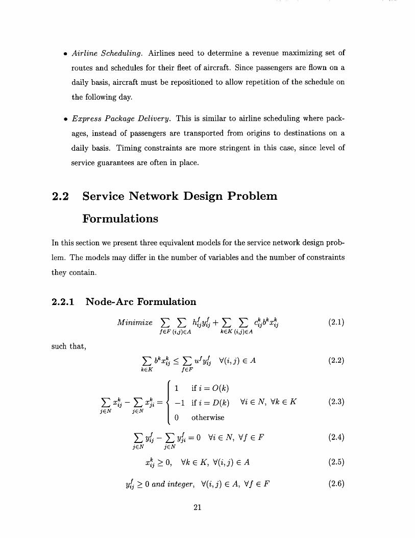
2.2.1 Node-Arc Formulation
Minimize h -y~y + c b k. (2.1)fEF (i,j)EA keK (i,j)EA
such that,
Z bkxk <k ufy V(i,j) E A (2.2)keK fEF
1 if i = O(k)
xi - x i = -1 if i= D(k) Vi E N, Vk E K (2.3)jEN jEN
0 otherwise
yi - yfi 0 Vi E N, V f F (2.4)jEN jEN
xi 0, Vk E K, V(i,j) c A (2.5)
y > 0 and integer, V(i,j) E A, Vf E F (2.6)
The objective (2.1) is to find the cost minimizing deployment of assets and routing
of flows on the network constituted by the assets subject to constraints (2.2) - (2.6).
Constraints (2.2), the forcing constraints limit the amount of flow on any are to the
capacity of that arc, as determined by the value of design variables. Constraints (2.3)
are the flow conservation constraints that ensure that each commodity is fully ser-
viced from its origin to destination. Constraints (2.4) are design balance constraints
that distinguish service network design problems from conventional network design
problems. Constraints (2.5) ensure non-negativity of commodity flows and constraints
(2.6) ensure the integrality and non-negativity of design variables.
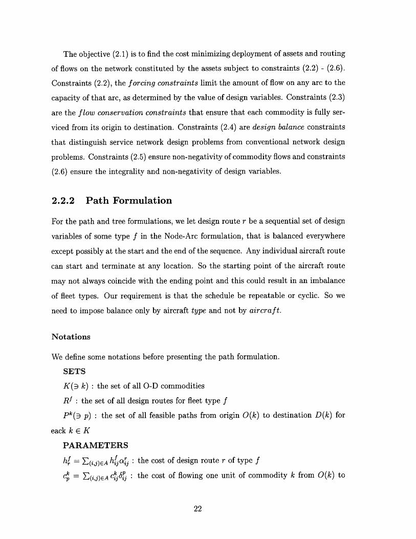
2.2.2 Path Formulation
For the path and tree formulations, we let design route r be a sequential set of design
variables of some type f in the Node-Arc formulation, that is balanced everywhere
except possibly at the start and the end of the sequence. Any individual aircraft route
can start and terminate at any location. So the starting point of the aircraft route
may not always coincide with the ending point and this could result in an imbalance
of fleet types. Our requirement is that the schedule be repeatable or cyclic. So we
need to impose balance only by aircraft type and not by aircraft.
Notations
We define some notations before presenting the path formulation.
SETS
K(3 k) : the set of all O-D commodities
Rf : the set of all design routes for fleet type f
pk(3 p) : the set of all feasible paths from origin O(k) to destination D(k) for
eack k E K
PARAMETERS
hf = E(i,j)CA hja : the cost of design route r of type f
c = E(i,j)EA ci6j : the cost of flowing one unit of commodity k from O(k) to

D(k) along path p E pk
INDICATOR VARIABLES
S 1 if design variable for (i, j) is included in design route r
0 otherwise
1 if i E N is the start node of design route r
i - 1 if i E N is the end node of design route r
0 otherwise
6? = 1 if arc (i, j) belongs to path p{ 0 otherwise
DECISION VARIABLES
yf : number of assets of type f deployed on design route r
z : fraction of bk on path p E pk for all k E K
With these notations we present the path formulation below (see Ahuja et al. [3]
for demonstration of equivalence between Node-Arc and Path formulations).
SNDP-Path
Minimize hf y + (ckbk )x k (2.7)rERf kEK pEPk
such that,
E S (bk)x < ufyfa , V(i,j) E A (2.8)kEKpEPk fEF rERf
x=1 , Vk E K (2.9)pEP
C yf = 0 , Vi E N, VfE F (2.10)rERI
xk > 0 Vp E P k, Vk E K (2.11)
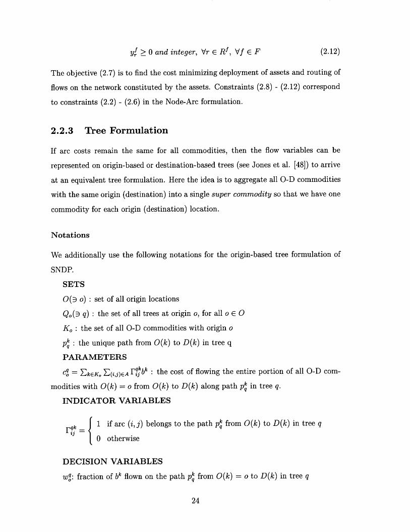
y{ > 0 and integer, Vr E Rf, Vf E F
The objective (2.7) is to find the cost minimizing deployment of assets and routing of
flows on the network constituted by the assets. Constraints (2.8) - (2.12) correspond
to constraints (2.2) - (2.6) in the Node-Arc formulation.
2.2.3 Tree Formulation
If arc costs remain the same for all commodities, then the flow variables can be
represented on origin-based or destination-based trees (see Jones et al. [48]) to arrive
at an equivalent tree formulation. Here the idea is to aggregate all O-D commodities
with the same origin (destination) into a single super commodity so that we have one
commodity for each origin (destination) location.
Notations
We additionally use the following notations for the origin-based tree formulation of
SNDP.
SETS
O(E o) : set of all origin locations
Qo (3 q) : the set of all trees at origin o, for all o E O
Ko : the set of all O-D commodities with origin o
pk : the unique path from O(k) to D(k) in tree q
PARAMETERS
cq = -kEKo (i,j)EA Fqkbk : the cost of flowing the entire portion of all O-D com-
modities with O(k) = o from O(k) to D(k) along path pq in tree q.
INDICATOR VARIABLES
1 if arc (i, j) belongs to the path pk from 0(k) to D(k) in tree q
0 otherwise
DECISION VARIABLES
wtq: fraction of bk flown on the path pk from O(k) = o to D(k) in tree q
(2.12)

SNDP-Tree
Minimize Z h y! + ~ cqw q (2.13)rERI oEO qEQo
such that,
{ (E I w _bk yf uy , V(i,j) E A (2.14)oEO qEQo kEKo fEF rERf
w g = 1, VoEO (2.15)qEQo
Z yf =0 , Vi E N, Vf E F (2.16)rERI
wq 2 0, Vq E Q, Vo E O (2.17)
yf 0 and integer, Vr E Rf, Vf E F (2.18)
The objective (2.13) is to find the cost minimizing deployment of assets and rout-
ing of flows on the network constituted by the assets. Constraints (2.14) - (2.18)
correspond to constraints (2.2) - (2.6) in the Node-Arc formulation.
2.2.4 Comparison of Formulations
Compared to SNDP - Node - Arc the number of flow conservation constraints in
SNDP - Path is reduced from INI x |KI to IKI. In the tree formulation this number
is further reduced to 101, the number of origin locations. The reduction in the number
of constraints makes the path and tree formulations particularly amenable to large
scale problems. We refer the reader to Ahuja et al. [3], Jones et al. [48] and Kim [52]
for a discussion on the advantages of path and tree formulations over the node-arc
formulation. However, the number of variables increases exponentially in the path
and tree formulations. In Chapter 3, we outline some solution methods for problems
with a large number of decision variables. Table (2.1) summarizes the differences in
the number of flow conservation constraints and the number of decision variables
among the three formulations.
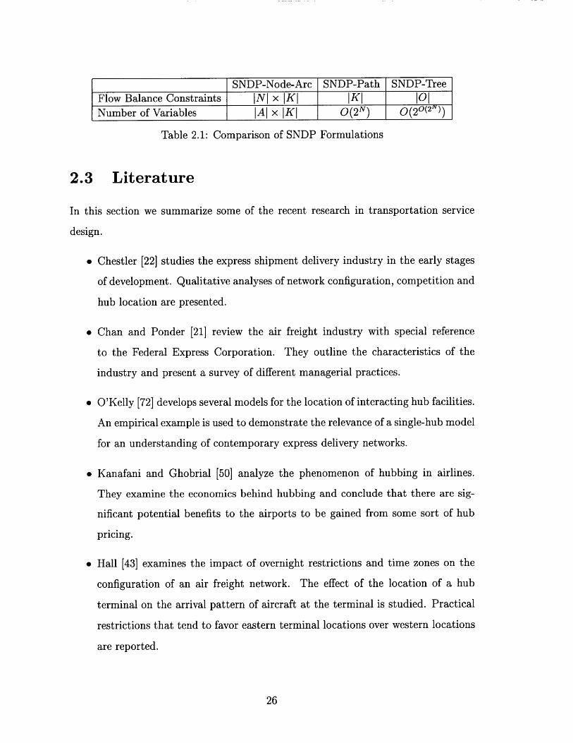
SNDP-Node-Arc SNDP-Path SNDP-TreeFlow Balance Constraints INI x IKI IKI 101Number of Variables JAl x IKI O( 2N) O(20(2"))
Table 2.1: Comparison of SNDP Formulations
2.3 Literature
In this section we summarize some of the recent research in transportation service
design.
* Chestler [22] studies the express shipment delivery industry in the early stages
of development. Qualitative analyses of network configuration, competition and
hub location are presented.
* Chan and Ponder [21] review the air freight industry with special reference
to the Federal Express Corporation. They outline the characteristics of the
industry and present a survey of different managerial practices.
* O'Kelly [72] develops several models for the location of interacting hub facilities.
An empirical example is used to demonstrate the relevance of a single-hub model
for an understanding of contemporary express delivery networks.
* Kanafani and Ghobrial [50] analyze the phenomenon of hubbing in airlines.
They examine the economics behind hubbing and conclude that there are sig-
nificant potential benefits to the airports to be gained from some sort of hub
pricing.
* Hall [43] examines the impact of overnight restrictions and time zones on the
configuration of an air freight network. The effect of the location of a hub
terminal on the arrival pattern of aircraft at the terminal is studied. Practical
restrictions that tend to favor eastern terminal locations over western locations
are reported.
* Kuby and Gray [54] compare the cost-effectiveness of hub-and-spoke networks
with stopovers and feeders to that of pure hub-and-spoke networks and present
a case study on Federal Express. They assume a single sorting hub and a
relatively small market covering only the western United States and develop a
mixed integer program to design the least-cost air network.
* Barnhart and Schneur [18] develop a model and algorithm for an express ship-
ment service network design problem. In their model, (1) there is only one hub,
(2) transfer of shipments between aircraft at gateways in disallowed and (3)
only one type of aircraft is allowed to serve each gateway location. The upshot
is that shipment routings are completely determined by aircraft routes.
* Kamoun and Hall [49] analyze the express mail delivery problem for the courier
services industry. These companies operate like taxi companies, but transport
mail and packages instead of people. Kamoun and Hall propose two new de-
signs without using linear programming techniques and provide results based
on simulation.
* Kim [52] develops generic models and algorithms for large-scale transportation
service network design problems and illustrates an application in the express
package delivery industry. By exploiting special problem structure and applying
novel problem reduction techniques, a dramatic decrease in problem size is
achieved without compromising exactness of the model.
* If we consider the NDP with a single source node e and a fixed capacity uij = U
on all arcs and add assignment constraints,
y,= 1 ,ViEN\ {e}jEN
Yij= 1 ,Vj E N\{e}iEN
as well as the constraint,
SYej < n,iEN
the NDP becomes a vehicle routing problem (VRP) for a homogeneous fleet of n
vehicles each domiciled at depot e and each having a capacity U. Comprehensive
surveys by Magnanti [59], Magnanti and Wong [64], Golden and Assad [42]
Desauliniers et al. [30] and Desrosiers et al. [32] summarize the developments
in this field.
* Talluri and Gopalan [85] survey various mathematical models in airline schedule
planning. Barnhart et al. [17] and Shenoi [83] present integrated models and
solution techniques for airline planning including integrated fleet assignment and
maintenance routing, and integrated crew scheduling and deadhead selection.
Daskin and Panayotopoulos [29] analyze the probem of assigning aircraft to
scheduled routes to maximize profits in passenger hub and spoke networks. A
Lagrangian relaxation of the formulation is outlined together with heuristics for
converting Lagrangian solutions into primal solutions and for improving on the
solutions.
* In the railroad industry, Ziarati et al. [91] develop models for assigning loco-
motives to trains to operate a given schedule. They solve the models using a
Dantzig-Wolfe decomposition technique, where subproblems are formulated as
constrained or unconstrained shortest path problems. Newton [71] and Barn-
hart et al. [14] study network design problem with budget constraints with an
application to railroad blocking problems.
* Powell [74] models the load planning problem for Less-Than-Truckload (LTL)
motor carriers as a Service Network Design Problem. A local improvement
heuristic is proposed which adds and drops links to and from the network in
an intelligent sequence. After each change, the routing of freight over the net-
work is approximately reoptimized. Farvolden and Powell [33] present local-
improvement heuristics for a SNDP encountered in LTL common carrier appli-
cations. The add/drop heuristics are based upon subgradients derived from the
optimal dual variables of the shipment routing subproblem that is modeled as a
multicommodity network flow problem. The basis of the multicommodity net-

work flow problem is partitioned to facilitate the calculation of dual variables,
reduced costs and subgradients (see Farvolden et al. [34]). Powell and Sheffi
[75] also use add/drop heuristics for LTL motor carrier applications.
Wong [89] raises some algorithmic and computational questions in transporta-
tion network research. Possible advances in improving the quality of solutions,
increasing the size of problems that can be handled and use of approximate
procedures are suggested.
Most of the previously developed models and solution techniques have been used to
solve small and medium scale real-life problems (see Kim [52] for details). In the next
section we identify the needs to solve very large scale real-life problems and present
an overview of our solution approach.
2.4 Decomposition Solution Approach
We recall that the service network design problem has two kinds of decision variables,
one for the deployment of transportation assets onto network paths and the other
for the routing of shipments over the network. Simultaneous solution for both these
types of variables for many transportation applications requires hardware capabilities
that are far greater than those available to most transportation service providers. As
the size of the problem increases, it might take hours of runtime just to discover that
there is not enough memory in the system to solve the problem. This time consuming
process often yields very little insight into the problem. Hence there is a pressing need
for a procedure that allows us to solve very large-scale transportation applications.
Our solution approach strives to satisfy this need by using two models, each dealing
with a subproblem for one kind of decision variable, in an iterative framework that
integrates results from both the models. We use an approximate service network
design model, called SNDP-Approx, to generate routes for transportation assets and
a variant of integer multicommodity flow models, called LEM, to generate shipment
flows.

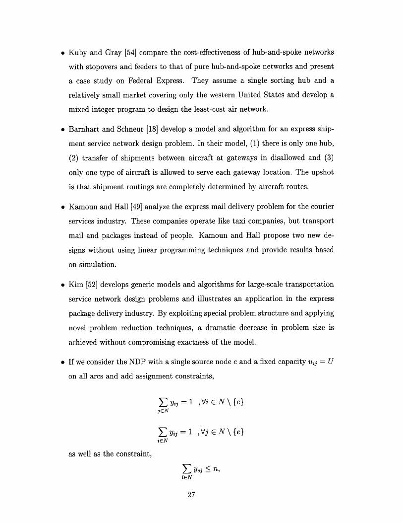
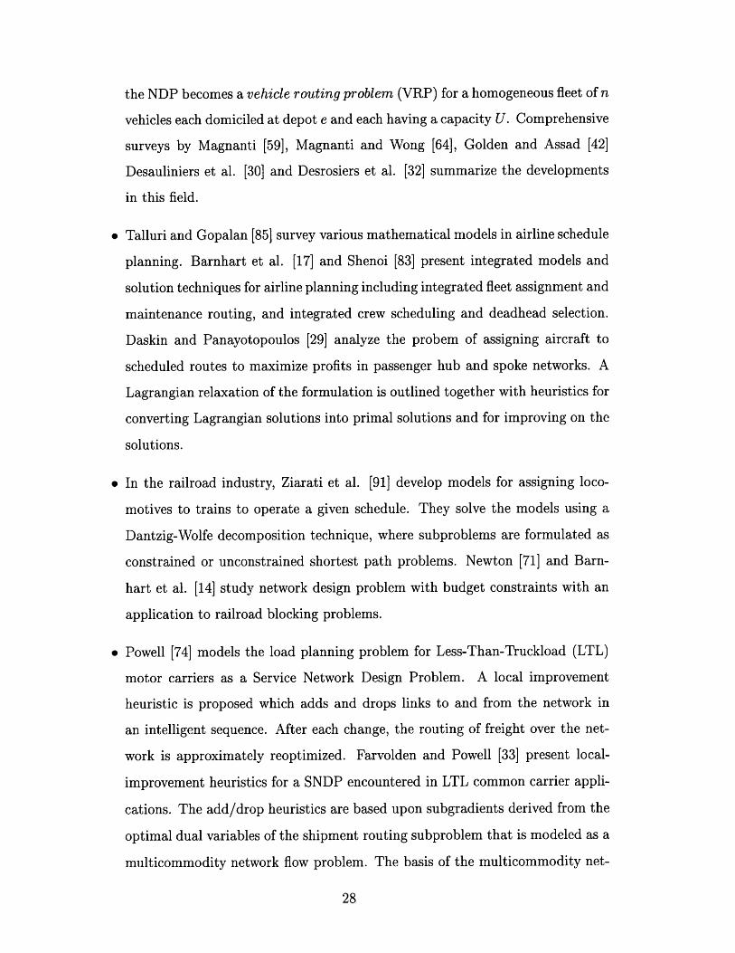
2.4.1 Decomposition Algorithm
We first generate routes for transportation assets by using the route generation model,
SNDP - Approx. On the network constructed from these routes, we flow shipments
in an intelligent manner using the shipment flow model, LEM, and based on these
shipment flows we fix some of the routes and strip out the shipments that can be
serviced by the routes selected so far. We repeat this procedure with the shipments
remaining to be serviced. This way the number of shipments that need to be serviced
is successively reduced so that in the end we either have a set of selected routes
that have enough capacity to service all the shipments or a small enough number of
shipments that the problem can be solved using exact models without computational
burden.
Our solution approach can be outlined as follows:
0. Initial Input: Input all commodity demand data, locations, ca-
pacities, costs and initialize the set of selected routes to a null-set. Go to
Step 1.
1. Route Generation: Solve the model SNDP - Approx with the
input set of commodities and generate "promising" routes for transporta-
tion assets.
2. Shipment Flow Generation: Solve LEM and arrive at a set
of commodity flows over the service network generated in the Route
Generation step.
3. Variable Fixing : Augment the set of selected routes by fixing
some of the promising routes generated in the Route Generation step.
The selected routes are those that are very likely to be in the optimal
solution and are identified based on the flows from the Shipment Flow
Generation step. We provide more details in Chapter 5.
4. Feasibility Check: Verify using LEM if the service network
formed by the current set of selected routes has enough capacity to carry
all demand. If yes, STOP; else go to the Problem Size Reduction step.

5. Problem Size Reduction: Eliminate commodities that can be
moved on the service network formed by the set of selected routes. If the
service design problem for the remaining commodities is small enough to
solve exactly with available hardware, solve using the service network de-
sign model (detailed in Section 2). Otherwise, go to the Route Generation
step with the remaining set of commodities as input.
A key idea of our approach is that we keep selecting routes and flowing commodi-
ties at each step until the size of the problem with the remaining commodities is small
enough to be solved exactly with current memory availability or we have a feasible
solution. This greatly enhances the tractability of our solution technique. The flow
chart corresponding to our algorithm is shown in Figure 2-1.
2.4.2 Shipment Flow Model Description
We now introduce a variant of integer multicommodity flow models called the Location
Elimination Model (LEM) to flow shipments in such a way as to reduce the size of
the subproblem at the next iteration. In Chapter 4, we describe LEM in detail.
The motivation for LEM arises from the fact that the routes generated in the Route
Generation step of our solution approach may not have enough capacity to move the
entire demand for shipments from their origins to their destinations. Hence there is a
need for a model that can flow some of the shipments on such a network that does not
have enough capacity and aid the overall solution algorithm in making some decisions
based on the shipment flow patterns. LEM establishes a set of commodity flows on
the fleet network that maximizes the number of origin and destination locations for
which all demand originating at or destined for that location, as the case may be, is
assigned to network paths. If all origin and destination locations do not have their
entire demands assigned to the network, we can fix only the fleet routes that carry
the entire demand of origin or destination locations they visit. This results in the
following:
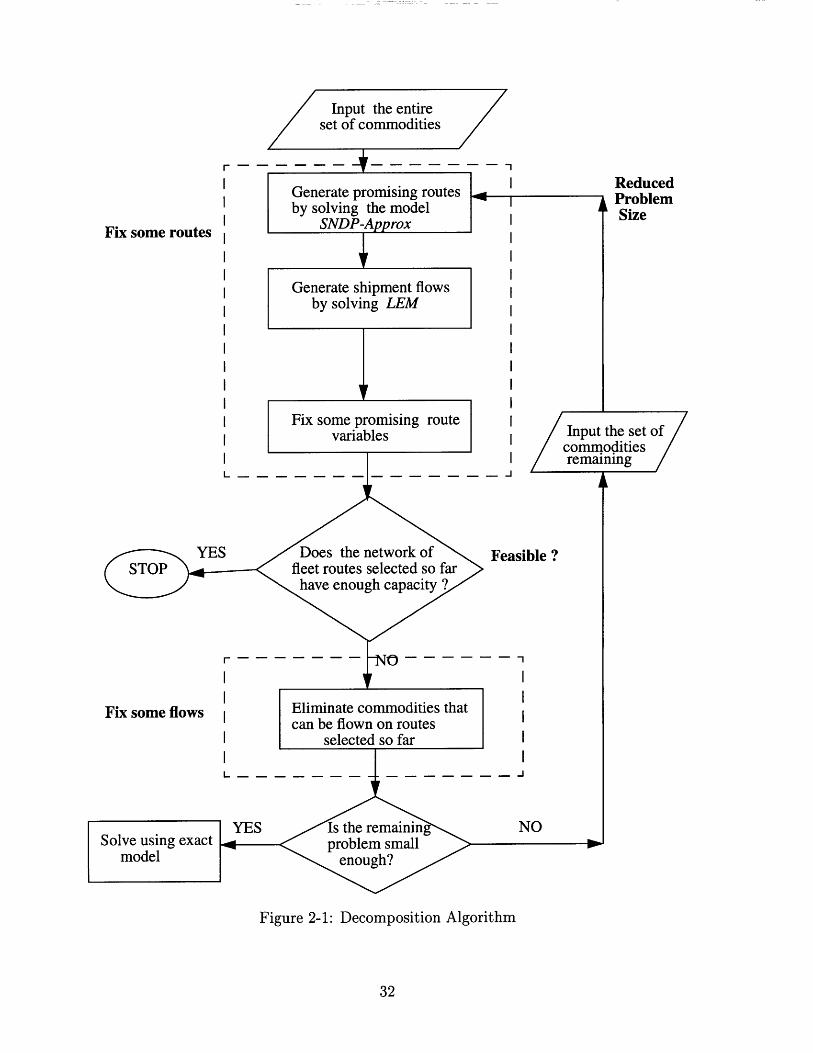
Input the entireset of commodities
----------- ----
Fix some routes
Generate promising routesby solving the model
SNDP-Approx
Generate shipment flowsby solving LEM
Fix some promising routevariables
ReducedProblemSize
Input the set ofcommoditiesremainingI I/
YES Does the network of Feasible ?STOP fleet routes selected so far
have enough capacity ?
r - - - - - - - - - - - - -
Fix some flows Eliminate commodities thatcan be flown on routes
selected so farI IL - - - - - - - - - - - - - - j
YES Is the remaining NOSolve using exact problem small
model enough?
Figure 2-1: Decomposition Algorithm
* The number of O-D commodities, whose demand is satisfied is reduced. This
translates into a reduction in the size of input data for the Route Generation
problem in the next iteration.
* There is an elimination of some origin and destination locations whose demand
has been entirely moved. This results in a corresponding reduction in the size
of the fleet network in the Route Generation step.
LEM can be used either in a stand-alone fashion or embedded in an iterative
framework for solving large scale problems. If all origin and destination locations
have their entire demands assigned to the network, we can infer that there is enough
capacity in the network to carry all O-D demand. Thus LEM can be used as a
stand-alone model to check the feasibility of any solution to the NDP with respect to
demand.
The elimination of some origin and destination locations might result in a consid-
erable reduction in the size of the fleet network in the Route Generation step, since
many transportation applications involve time as a factor and every single physical
location will correspond to multiple nodes in a network in space and time. Thus LEM
is intelligent because it flows shipments in a way that reduces problem size for future
consideration.

Chapter 3
Routing for Transportation
Service Network Design:
Models and Solutions
In this chapter we describe the first type of subproblem that deals with arriving at
a routing plan for the transportation assets or fleet. We use approximate service
network design models to solve this problem. We first present approximate SNDP
models after providing some necessary background. We then present a brief review
of literature followed by some solution techniques for solving large scale problems.
3.1 Valid Inequalities
Given some values for the design variables y, thereby determining the capacities on
the arcs, the SNDP has a feasible flow of bk from O(k) to D(k) only if the capacity of
every O(k) - D(k) cutset is at least bk. In general, for any feasible solution to SNDP,
the aggregate capacity across the cutset must be no less than the demand across the
cutset. These aggregate capacity demand inequalities (see Magnanti et al. [62]) are
expressed as:
E Uf YT DS,T , for all O - D cutsets {S,T} (3.1)fEf
where we define cutset {S, T} to be a partition of the node set N into two mutually
exclusive and collectively exhaustive non-empty subsets S and T = N \ S. We letYf = (ij)6A Y in the Node-Arc formulation and Yf f -rE (i,) {ST}nr Y in
S,T =(ij)EA Yij 'T =ErERf Z(ij)ES,T}flr yi
the route-based formulation. We let DS,T be the total demand of all commodities
with origin in subset S, i.e. O(k) E S and destination in subset T (D(k) E T).
Inequalities (3.1) are knapsack inequalities that can be strengthened in many ways.
One way is to use rounding that results in Chv&tal - Gomory cuts. Alternatively we
could generate cutset inequalities as explained in Magnanti et al. ([62] and [61]) and
Magnanti and Mirchandani [60]. Also see Stoer [84] for details on valid inequalities.
3.1.1 Chvatal-Gomory Cuts
The aggregate capacity demand inequalities (3.1) can be lifted by applying simple
integer rounding to produce Chvatal - Gomory (C-G) cuts. If we let I be a particular
asset or service type then the following C-G cuts are valid for each O-D cutset {S, T}.
S ] YS,[T > 1 ,V 1 E F, for all 0 - D cutsets {S,T} (3.2)
We refer the reader to Nemhauser and Wolsey [70] for further details. The difficulty
in using C - G cuts is that there are exponentially many. For instance, in the case of
N origin locations and F fleet types, the total number of C - G cuts including the
aggregate capacity demand inequalities is { 2 (2N - 1)} x (IFI + 1).
3.1.2 Cutset Inequalities
The aggregate capacity demand inequalities (3.1) can be alternatively strengthened
by using cutset inequalities. Cutset inequalities, extensively researched by Magnanti,
Mirchandani and Vachani ([62] and [61]) and Magnanti and Mirchandani [60], may
provide tighter LP bounds than C-G cuts. We assume that there are only two service
or asset types for ease of exposition. However, they can be generated for more than
two types. The cuts (3.1) can be written as:
uLYJT + U2 S2T > DS,T (3.3)
and the two types of cutset inequalities can be written as:
1T 2 , (3.4),T + r(Ds,T,U1 ) u (3.4)
1 1 YV > ](3.5)r(Ds,T, 2) S,T S,T - (3.5)
where r(Ds,T, u) DS,T - ( )The generalized version of cutset inequalities can be found in Magnanti et al.
[62]. As with the C - G cuts, the number of cutset inequalities grows exponentially
with the number of locations. For example, in the case of N origin locations and F
fleet types, the total number of cutset inequalities including the aggregate capacity
demand inequalities is { 2 (2N - 1)} x (IF+ 1), which is the same as that for C-G cuts.
3.2 The Approximate Service Network Design
Cutset Model
When the costs of flow variables are negligible compared to fixed design variable
costs, we can approximate the network design problem without considering flows
explicitly. When there is only one commodity, we can show using a max - flow min -
cut argument that aggregate capacity demand inequalities are both necessary and
sufficient, to guarantee a feasible single-commodity solution (see Ahuja et al. [3] for
details). For multicommodity problems, aggregate capacity demand inequalities are
a necessary, but not a sufficient, condition to guarantee a feasible multicommodity
flow solution (for example, see Mirchandani [67]). Because SNDP involves multiple
commodities, we approximate SNDP with SNDP-Approx. Correspondingly we call
the approximation of SNDP - Node - Arc as SNDP - Approx - Node - Arc and that
the approximation of SNDP - Path and SNDP - Tree as SNDP - Approx - Route.
SNDP-Approx models enable us to solve SNDP approximately, considering only the
design variables and ignoring the huge number of flow variables and large number of
constraints (flow balance and forcing constraints) associated with the flow variables.
3.2.1 Approximate SNDP Formulations
We present below the approximate node-arc and route-based formulations.
SNDP-Approx-Node-Arc
Minimize C hfyfj (3.6)fEF (i,j)EA
such that
SUf Y!T, > DS,T , V O - D cutsets {S, T} (3.7)fef
y - yf = 0 Vi E N, V f F (3.8)jEN jEN
yf. > 0 and integer, V(i, j) E A, Vf E F (3.9)
SNDP-Approx-Route
Minimize 5 h{yf (3.10)rERf
such that
SufYsT', DS,T , V 0 - D cutsets {S, T} (3.11)fEf
Pryf = 0 , Vi E N, Vf E F (3.12)rERf
yf o0 and integer, Vr E Rf, Vf E F (3.13)

3.3 Literature
Cutset based formulations have been used in the literature to model variants of NDP
such as the survivable network design problem, Steiner tree problems, location-design
and location-routing problems, point-to-point routing problems etc. Goemans and
Williamson [40] outline several of these problems and summarize the research in
approximation algorithms for solution to these problems. Stoer [84] presents a study
on existing cutset models, decomposition solution techniques, valid inequalities and
lifting theorems for the design of survivable networks. In transportation, Kim [52]
presents an application of cutset models for express shipment delivery.
3.4 Solution Approach
In this section we present a generic solution to large-scale integer programs with a
prohibitively huge number of variables and constraints. Direct solution to these prob-
lems is usually not possible even with state-of-the-art LP/IP solvers (such as CPLEX
[26] , MINTO [69] , OSL [47]). We first present a solution technique for large-scale
linear programs that is based on variable restriction and constraint relaxation. We
then present a solution technique for integer programs that is based on variable re-
striction and constraint relaxation embedded within a Branch-and-Bound framework.
We provide details of specific techniques for our application in Chapter 5.
3.4.1 LP solution
Column Generation
When a linear program contains an exponential number of variables (or columns)
rendering a direct solution very difficult, we resort to Dantzig-Wolfe decomposition
[28] or Column Generation solution techniques. The key idea is to start with a very
small number of decision variables from the original formulation called the Master
Problem (MP) to form a smaller problem called the Restricted Master Problem
(RMP), that is solved to optimality. To check the optimality of a solution to RMP
with respect to MP, a subproblem called the pricing problem is solved. The result is
that either optimality is proved or new variables whose inclusion into the RMP might
improve the solution quality are identified. If such variables are found, the RMP is
re-optimized. The entire process is repeated until optimality of the MP is proved.
The ease with which the pricing subproblem is solved determines tractability of the
column generation procedure. Column generation can be either implicit or explicit.
Implicit column generation refers to solving the pricing subproblem without evalu-
ating all variables (e.g., by solving an optimization problem of some kind such as
the shortest path problem), whereas explicit column generation refers to solving the
pricing subproblem by calculating the reduced cost of all variables.
Row Generation
Row generation is the dual analogue of column generation for LPs with a huge num-
ber of constraints. The idea is to start with a very small number of constraints from
the MP to form a smaller problem called the relaxed problem (RP), that is solved to
optimality. To check the optimality of a solution to RP with respect to MP, a sub-
problem called the separation problem is solved, that identifies violated constraints
(rows) to add to the current RP. If such constraints are found, the RP is re-optimized.
The entire process is repeated until no violated constraints are found. Row generation
can be either explicit or implicit. Explicit row generation is necessary when there is
no efficient algorithm to solve the separation problem and violated constraints may
be identified by evaluating each constraint. Implicit row generation refers to the case
when there is an algorithm to solve the separation problem.
When there is a single commodity, the task of identifying the most violated cut-
set inequalities, called the cutset separation problem, by max-flow min-cut duality,
reduces to identifying the min-cut. For the case with multiple commodities, there is
no efficient procedure to solve the cutset separation problem (see Balakrishnan et al.
[5]). Leighton and Rao [56] present an approximate max-flow min-cut theorem for a
special kind of multicommodity flow problem called the uniform multicommodity
flow problem. Linial et al. [58] present an approximate max-flow min-cut theorem

for a general multicommodity flow problem and provide an approximation algorithm
for the cutset separation problem. They use the technique of embedding metrics for
the multicommodity cut problem. Williamson et al. [88] and Gabow et al.[37] solve a
cutset separation problem as an intermediate step in an approximation algorithm for
the survivable network design problem. They demonstrate how to solve the separation
problem efficiently for special cases that could arise in telecommunication.
Synchronized Column and Row Generation
To solve LPs with both a huge number of variables and a huge number of constraints,
it may be necessary to use both column and row generation. The idea is to start with
a small number of columns (variables) and rows (constraints) from the original master
problem MP, to form the RMP. One approach is to perform column generation until
all columns have non-negative reduced costs. Then this is followed by row generation
until no violated constraints are identified. After completing row generation, the
entire process is repeated. The algorithm terminates when there are both no columns
and no violated constraints to add. The challenge in implementing such a procedure is
in adding constraints that do not change the structure of the pricing subproblem and
adding columns that do not change the structure of the separation subproblem. This
is averted however, if we use explicit column generation and explicit row generation.
The difficulty is that explicit generation may be computationally expensive or even,
impractical. The growth of the size of RMP is illustrated in Figure 3-1.
3.4.2 IP solution
Branch-and-Bound is a divide-and-conquer solution technique (refer to Cormen
et al. [25]) to solve IPs by solving a series of LP subproblems (see Nemhauser and
Wolsey [70] and Bradley et al. [20]). When the problem contains a huge number of
decision variables, a technique called Branch - and - Price that integrates features
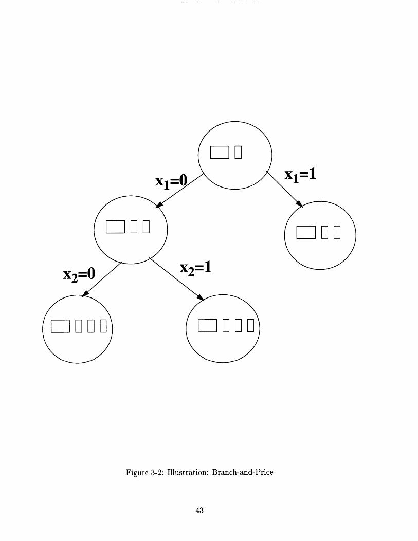
of both Column Generation and Branch-and-Bound, is used (see Figure 3-2). The
major challenge of Branch-and-Price is to devise branching rules that maintain an

5
Figure 3-1: Illustration: Synchronized Colummn and Row Generation
efficient structure of the pricing subproblem (see Barnhart et al. [16]). We refer the
reader to Parker and Ryan [73], Desrosiers et al. [32], Vance et al. [87], Barnhart
et al. [16] and Desrochers and Soumis [31] for alternative branching strategies for
different types of problems.
When the problem contains a huge number of constraints, a Branch - and -
Cut technique can used. Branch-and-Cut integrates Branch-and-Bound and Row
Generation by using Row Generation (or Cut Generation) in solving LPs at each
node of the Branch-and-Bound tree. Branching occurs when no violated constraints
are found. The difficulty is in developing an algorithm to solve the separation problem.
For problems with huge number of both columns and rows, Branch-and-Price and
Branch-and-Cut can be integrated to form a Branch - and - Price - and - Cut
solution technique. However, incompatibility between row and column generation
steps often make it difficult to solve IPs using Branch-and-Price-and-Cut. Barnhart
et al. [16] present heuristic approaches that may be able to provide a good integer
solution.
X1
x2=1
Figure 3-2: Illustration: Branch-and-Price
Xl=1
X2:
Chapter 4
Shipment Flow Problem:
Models and Applications
In this chapter we describe the second type of sub-problem that deals with the decision
of commodity routing over a given fleet network with finite arc capacities. Such
problems belong to a general class of network flow problems called Multicommodity
Flow (MCF) problems. Because of their interesting mathematical properties and
wide applicability, MCF problems have been extensively studied. We first outline
some generalities of the MCF problem before presenting our model.
4.1 Baseline Multicommodity Flow Problem
Formulation
The multicommodity flow problem is a subproblem embedded in the Network Design
Problem. When the design variables in the NDP model (as presented in Chapter
1) are fixed, only decisions on the flow variables remain and the problem reduces to
finding a minimum cost routing of commodities from their origins to destinations over
the network formed by design variables. If we assume uij to be the capacity on arc
(i, j) E A after fixing the design variables, then the resulting MCF problem can be
formulated as:

Minimize E EC cbkx (4.1)kEK (i,j)EA
such that
Sbkx. u ij V(i, j) E A (4.2)kEK
1 if i = O(k)
xj - ji= -1 if i= D(k) Vi E N, Vk E K (4.3)jEN jEN
0 otherwise
x > 0, Vk E K, V(i,j) E A (4.4)
The objective (4.1) is to find a minimum cost routing of commodities from their origins
to destinations over the network. Constraints (4.2) are called bundle constraints
that limit the amount of flow on any arc to its capacity. Constraints (4.3) are flow
conservation constraints that ensure that each commodity is fully serviced from
origin to destination. Constraints (4.4) guarantee non-negativity of flow variables.
4.2 Applications of Multicommodity Flow
Models
Multicommodity flow problems have a number of applications in various areas like
transportation, logistics, telecommunication, production, etc. Some of the applica-
tions are presented in this section.
4.2.1 Transportation and Logistics
Some applications of MCF problems in transportation and logistics are described
below.
* Routing vehicles in Traffic networks(Dynamic Traffic Assignment). This
involves the determination of minimum delay routes for vehicles from their ori-
gins to their respective destinations over the traffic network. The allowable
congestion levels determine the arc capacities. Alternatively, there are no ca-
pacities but the cost on an arc is a function of the amount of flow on the arc.
* Airline Fleet Assignment. Given a time table of flight arrivals and departures,
the expected demand on the flights and a set of aircraft, the objective is to arrive
at a minimum cost assignment of aircraft to the flights. This problem has been
extensively studied (see Abara [1] and Hane et al. [44]).
* Aircraft Maintenance Routing. Given an assignment of flights to fleets, the
task is to determine a sequence of flights, or routes, starting and ending at
maintenance stations or to find rotations (cycles) in the network, to be flown
by individual aircraft so that all the flight legs are covered. This problem has
been studied by Barnhart et al. [11] Clarke et al. [23], Shenoi [83] and Feo and
Bard [35].
* Airline Crew Scheduling. This problem deals with minimum cost pairing of
crews and aircraft. Factors such as aircraft type compatibility, hours of work
limitations and Federal Aviation Administration (FAA) regulations must be
taken into account while solving the problem. For an in-depth study the reader
is referred to Anbil et al. [4] and Barnhart et al. [15].
* Distribution systems planning. In this problem there are different commodi-
ties produced at several plants with known production capacities. Each com-
modity has a certain demand in each customer zone. The demand is satisfied by
shipping via regional distribution centers (DCs) with finite storage capacities.
The problem of routing the commodities from the manufacturing plants to the
customer zones through the DCs can be formulated as a MCF problem.
* Import and export models. One of the factors that may affect export is handling
capacity at ports. Barnett, Binkley and McCarl [9] uses a MCF model to analyze
the effect of US port capacities on the export of wheat, corn and soybean.
* Optimization of freight operations. Crainic, Ferland and Rousseau [27] de-
velop a MCF-based routing and scheduling optimization model that considers

the planning issues for the railroad industry. More recently, Newton [71] and
Barnhart et al. [14] study the railroad blocking problem using multicommodity
based formulations.
* Freight Assignment in the Less - than Truck load(LTL) industry. An LTL
carrier has to consolidate many shipments to make economic use of the vehicles.
This requires the establishment of a large number of terminals to sort freight.
Trucking companies use forecasted demands to define routes for each vehicle to
carry freight to and from the terminals. Once the routes are fixed, the problem
is to deliver all the shipments with minimum total service time or cost. This
problem can be formulated as a MCF problem.
* Express Shipment Delivery. Kim [52] models the shipment delivery problem
faced by express carriers like Federal Express, Unites States Postal Service,
United Parcel Service etc. as a MCF problem on a network in space and time.
4.2.2 Other Applications
We present below some other applications of MCF models:
* Routing messages in a communication or computer network. The network
consists of transmission lines. Each message request is a commodity. The
problem is to route the messages from origins to the respective destinations at
a minimum cost.
* Long - term hydro - generation optimization. The task in this case is to
determine the amount of hydro-generation at a reservoir in an interval of time,
that minimizes the expected cost of power generation over a period of time,
divided into several intervals. Nabonna [68] showed that this problem can be
modeled as a MCF problem with inflows given as probabilistic density functions.
* Forest Management. For each planning period, forest managers have to make
decisions concerning the land areas to be harvested, the volume of timber to
be harvested from these areas, the land areas to be developed for recreation

and the road network to be built and maintained in order to support both the
timber haulers and recreationists. This problem has been formulated as a MCF
problem by Helgason, Kennington [51] and Wong [45].
* Street planning. Foulds [36] introduced this problem and modeled it as a MCF
problem. The objective is to identify a set of two-way streets such that making
these streets one-way minimizes the total congestion cost in the network.
* Spatial price equilibrium(SPE) problem. This problem requires modeling con-
sumer flows within a general network. The SPE problem determines the op-
timum levels of production and consumption at each market and the optimal
flows satisfy the equilibrium property. Segall [81] models and solves the SPE
problem as a MCF problem.
For a more comprehensive description of applications we refer the reader to Schneur
[79], Ahuja et al. [3] and Kennington [51].
4.3 Multicommodity Flow Solution Techniques
The linear MCF problem is the most studied instance of MCF problems. A fairly
comprehensive survey of linear multicommodity flow models and solution methods is
presented in Ahuja et al. [3]. We describe below some of the recent results in this
area.
* Saviozzi [78] uses subgradient techniques on the Lagrangean relaxation of the
bundle constraints and proposes a method of arriving at an advanced start-
ing basis for the minimum cost multicommodity flow problem. Depending on
whether the basis is primal feasible or dual feasible, further iterations can be
carried out with primal or dual simplex method, as the case may be.
* Barnhart and Sheffi [19] present a network-based heuristic solution strategy in
a primal-dual framework for MCF problems. This procedure is designed for
large-scale problems, whose size is excessive for the simplex or barrier methods.
* Barnhart et al.[13] present a cycle-based formulation of the MCF problems.
They also describe a partitioning solution procedure for large-scale MCF prob-
lems based on both column generation and constraint relaxation.
* Schneur [79] describes a procedure that uses the concepts of C-optimality (see
Ahuja et al. [3]) and scaling, together with a quadratic penalty function for the
capacity constraint, to solve the linear MCF problems.
* Barnhart [10] provides a dual-ascent heuristic for MCF problems that gives a
valid lower bound on the optimal primal objective value and an advanced start-
ing solution for primal-based solution methodologies. A heuristic to generate
an approximate primal-optimal solution is also described.
* Jones et al. [48] compare and contrast the different formulations of MCF prob-
lems. They present empirical evidence that the path-based formulation by de-
composition yields lower CPU times than the equivalent tree-based formulation.
* Radzik [76] considers one kind of MCF problem called the maximum concurrent
flow problem, where the objective is to design a set of commodity flows with
minimum possible congestion. The congestion of a given flow of commodities
is defined as the minimum number having the property that the flow is feasible
when all edge capacities are multiplied by this number. Radzik demonstrates
how approximate solutions to this problem can be computed deterministically
using a number of single-commodity minimum cost flow computations.
* Klein et al. [53] develop approximation algorithms for the concurrent flow prob-
lem with uniform capacities. Leighton et al. [55] present generalized algorithms
that are valid for problems with arbitrary capacities.
* Interior Point methods provide polynomial time algorithms for the MCF prob-
lems. The best time bound is due to Vaidya [86].
* Schultz and Meyer [80] provide an interior point method with massive parallel
computing to solve multicommodity flow problems.

* Zenios [90] presents an algorithm for nonlinear optimization problems with mul-
ticommodity flow constraints. Empirical results for a parallel implementation
are reported for quadratic programs with approximately 10 million columns and
100,000 rows.
4.4 Integer Multicommodity Flow Problems
4.4.1 Integer MCF Applications
In many applications of MCF models, each commodity is identified with a specific
origin and destination. In many cases, the demand for any commodity cannot be split
and assigned to multiple paths. Since MCF problems do not obey the integrality
property (see Ahuja et al. [3]), unlike pure network flow problems, it is necessary
to impose integrality requirements. These applications include the following (see
Barnhart et al. [16]):
* Bandwidth packing. This involves optimal allocation of bandwidth in telecom-
munication networks and routing of calls from their points of origins to their
destinations. In case of video teleconferencing, calls cannot be split and all O-D
demand should be routed on a single path.
* Express Package Delivery. In this problem that is mentioned before, often
it is desirable for all O-D demand to be routed on a single path to facilitate
operational ease and satisfy all the level of service requirements.
* Aircraft Maintenance Routing. In this problem mentioned before, each air-
craft is a commodity and aircraft should be assigned to paths such that each
flight is covered by exactly one aircraft.
4.4.2 Integer MCF Solution Techniques
Barnhart et al. [16] present a general solution strategy called Branch-and-Price, for
solving large-scale IPs. Branch-and-Price involves features from both Branch-and-
Bound and Column Generation. Researchers have tailored Branch-and-Price solution
techniques for solving different integer multicommodity flow models as follows:
* Barnhart et al. [12] study the large-scale Integer Multicommodity Flow Problem
in which the entire demand of any commodity is to be assigned to the same
path. They present a column generation model and Branch-and-Price-and-Cut
algorithm with specialized branching rules.
* Parker and Ryan [73] describe a Branch-and-Price algorithm for the bandwidth
packing problem in telecommunication networks. Bandwidth packing involves
the selection of a set of commodities to maximize revenue.
* Ziarati et al. [91] consider the problem of assigning railway locomotives to
trains. They model the problem as an integer multicommodity flow problem
with side constraints and solve using a Dantzig-Wolfe decomposition technique,
where subproblems are formulated as constrained or unconstrained shortest
path problems.
* Raghavan and Thompson [77] illustrate the use of randomized algorithms to
solve some integer multicommodity flow problems. They use randomized round-
ing procedures that give provably good solutions in the sense that they have a
very high probability of being close to optimality.
4.5 Location Elimination Model (LEM)
In this section we present a variant of a mixed integer multicommodity flow model,
called the Location Elimination Model (LEM), that was introduced in the context of
our decomposition solution approach in Chapter 2. We recall that LEM establishes
a set of commodity flows on the fleet network that maximizes the number of origin
and destination locations such that all demand originating at or destined for those
locations, as the case may be, is assigned to network paths. We let G = (N, A) be
the given fleet network over which commodities are to be flown, O the set of all
origin locations and D the set of all destination locations. Again, each commodity is
identified by a specific origin and destination pair. We let y, be a zero-one variable
for each origin o E O, that is equal to 1 if all the O-D commodities with O(k) = o are
assigned to network paths and equal to zero otherwise. Similarly we let Zd be a zero-
one variable for each destination d E D, that is equal to 1 if all the origin-destination
(O-D) commodities with D(k) = d are assigned to network paths and equal to zero
otherwise. The objective is to maximize
EoEo yo + EdED Zd
As with the multicommodity flow problem, the flow variables can be represented
on arcs and paths. Since we will be dealing with commodity independent arc costs,
we can also represent the flows on origin-based or destination-based trees, as has been
demonstrated by Jones et al. [48]. Since an arc based formulation has huge memory
requirements, we will consider only path-based and tree-based formulations.
4.5.1 LEM Path Formulation
Notations
Before presenting the path formulation, we first define some notations.
SETS
K(E k) : the set of all O-D commodities
pk(D p) : the set of all feasible paths from origin O(k) to destination D(k) for
eack k E K
Ko : the set of all O-D commodities with origin o
Kd : the set of all O-D commodities with destination d
Od : the set of all origins o such that there exists a commodity with O(k) = o and
D(k) = d, for each d E D
Do : the set of all destinations d such that there exists a commodity with O(k) = o
and D(k) = d, for each o E 0

PARAMETERS
bk : the demand for commodity for each k E K
uij : the capacity of arc (i, j) E A
INDICATOR VARIABLES
= 1 if arc (i, j) belongs to path p
0 otherwise
DECISION VARIABLES
x : fraction of bk on path p E pk for all k E K
The path formulation is as follows:
Maximize E Yo + E Zd (4.5)oEO dED
such that,
x k - yo|Do| > 0, Vo EO (4.6)keKo pEPk
SZxk - zdOd > , Vd ED (4.7)kEKd pEPk
k < 1, VkcK (4.8)pEPk
x k S x(6bk) < ui,, V(i,j) E A (4.9)kEK pEPk
zk > O (4.10)
yo, Zd E {0, 1} (4.11)
Constraints (4.6) ensure that a location cannot have all of its originating de-
mand served unless each commodity originating there is fully assigned to an origin-
destination path. Similarly we have constraints (4.7) for the destination locations.
Constraints (4.8) are generalized upper bounding constraints to ensure that the total
flow of any commodity k from O(k) to D(k) does not exceed its demand. Constraints
(4.9) represent the arc capacity constraints. Constraints (4.10) ensure that the path-
flows are non-negative. Constraints (4.11) imply that a location has either all of its
commodities served or it does not.
4.5.2 LEM Tree Formulation
Notations
Before presenting the tree formulation, we first define some more notations.
SETS
Qo(E q) : the set of all trees at origin o, for all o E O
Od : the set of all origins o such that there exists a commodity with O(k) = o and
D(k) = d, for each d E D
k : the unique path from O(k) to D(k) in tree q
INDICATOR VARIABLES
1 if arc (i, j) belongs to the path pk from O(k) to D(k) in tree q2 3 0 otherwise
DECISION VARIABLES
wq: fraction of bk flown on the path pk from O(k) = o to D(k) in tree q
The tree formulation is as follows:
Maximize Yo + E Zd (4.12)oEO dED
such that,
w - yo 0, Vo EO (4.13)qEQo
S wg - Zd IOd l _ O, Vd ED (4.14)oEOd qEQo
w q < l , VoEO (4.15)qEQo
{ ( r bk)W} < uij, V(i,j) E A (4.16)oEO qEQ kEKo
wg> , Vq E Qo, Vo E O (4.17)
Yo, Zd E {0, 1} (4.18)
Constraints (4.13) through (4.18) in the tree formulation correspond to constraints
(4.6) through (4.11) in the path formulation.
4.6 LEM LP Relaxation Solution
We will first consider solution to the linear programming relaxation of LEM. Our
approach to both the path and tree formulations will be based on Dantzig-Wolfe
decomposition [28] or Column Generation. The general approach is to start with
an initial subset of variables and generate more variables as needed by solving a
pricing subproblem. In our case, since the Yo and Zd variables are not too many in
number, we will start with all of them and generate only the flow variables by solving
the pricing subproblem.
4.6.1 Solution to the Path Formulation LP
We will generate the path flow variables x 's by solving the pricing problem. In
order to formulate the pricing problem, we will use the following vectors for the dual
variables:
A : duals corresponding to constraints (4.6)
p : duals corresponding to constraints (4.7)
a : duals corresponding to constraints (4.8)
7r : duals corresponding to constraints (4.9)
The pricing problem then can be written as follows:
p* = max{-Ao(k) - tD(k) - k ~- (6jbk)7r, }, Vk E K (4.19)pEpk (i,j)EA
or equivalently,
= - min{ AO(k) + D(k) + k + (6jb k)r},ppk (i,j)EA
Vk E K (4.20)
The reduced costs of all the path variables are non-positive if the following set of
conditions is satisfied:
- {AO(k) + I-lD(k) + 0 k + E (J6jbk)-i 0,(i,j)EA
Vp E pk, Vk e K (4.21)
Equivalently, optimality is reached if the following set of conditions is satisfied:
Vk e K (4.22)
The problem of determining the path that minimizes E(i,j)A (6 Jbk ) rij is a shortest
path problem for each k E K over the fleet network with modified arcs costs of 7rij (see
Ahuja et al [3]). That is, the pricing problem for the path formulation is solved by
finding a solution to an origin-destination shortest path problem for each commodity
k E K.
4.6.2 Solution to the Tree Formulation LP
We use the same notation for duals as the path formulation. The pricing problem is
formulated as:
p* = max{-A -qEQo SPd - -
dEDo,
Vo E 0 (4.23)E (K (ij)eA kkEK, (ij)EA
or equivalently,
p=- min{Ao + -d o+ Eo + E IqEQo dEDo kEKo (i,j)EA
min{ E (6jbk)irij} > -O(Aok) + ID(k) + 0k),PEPk (i,j)EA
(4.24)Vo E O.
Optimality is reached if the following set of conditions is satisfied:
S bk(min (F)rj}) -(A + d + ao) ,Vo e O. (4.25)qEQo --
kEK, (i,j)EA dEDo
The problem of finding the path that minimizes E(i,j)EA(FPq)7rij over all trees
q E Qo is a shortest path problem for each origin o E O and for each commodity
k E Ko over the fleet network with modified arcs costs of 7rij. That is, the pricing
problem for the tree formulation is solved by finding a solution to a single-origin
single-destination shortest path problem for the combination of each origin o E O
and each O-D commodity k E K,.
4.7 LEM IP Solution
Although integer multicommodity flow problems have been studied by many re-
searchers (see section 4.4), LEM is a very different kind of integer MCF problem
in that the demand for any commodity can be split between paths. Hence previously
developed Branch-and-Price techniques do not apply. We will use a variant of Branch-
and-Price in which simple branching is done on origin and destination variables, yo
and Zd, and the shortest path pricing subproblem is solved for the generation of flow
variables (xk and wg).
Chapter 5
Service Network Design for
Express Shipment Delivery:
A Case Study
In this chapter we demonstrate a successful application of our models and solution
techniques in the express shipment delivery industry, where consolidation occurs when
shipments are sorted at the hubs. We first describe the express shipment delivery
operation and the practical constraints that need to be considered while modeling
the decision problem. We then present a routing model and solution algorithm and
describe how we use our decomposition technique to solve this service network design
problem. We conclude this chapter with computational results.
5.1 Express Shipment Delivery Operation
In this section we describe the service network design problem of a large carrier in the
express shipment delivery industry. Our description is abstracted from Kim [52]. The
objective is to determine the cost minimizing movement of shipments (or packages)
from their origins to their destinations using a limited amount of resources, such that
all level of service (LOS) requirements are satisfied. There are multiple products
or service types, depending on the LOS requirements. Premium service that occurs
overnight is referred to as Next Day Service, while guaranteed service within 48
hours is called Second Day Service and service within 3-5 days is called Deferred
Service.
5.1.1 Problem Description
This service network design problem, like others, can be envisaged to consist of two
types of decisions: the first is to determine the service network formed by the routes
of transportation assets and the second is to determine shipment flows over the
service network. The service network is defined by the movements in space and time
of the transportation assets, in this case, aircraft and ground vehicles. The routes for
individual shipments from origins to destinations determine the flows on each link in
the service network.
Service Network and Shipment Flows
Shipments originate and terminate at locations, that could either be airports called
gateways or non-airport all ground locations, where they are loaded, unloaded and
transferred between aircraft and/or ground vehicles. From its initial gateway, a ship-
ment may be flown to at most one additional gateway before it is flown to a hub. Hubs
are specialized gateways or all ground locations, where shipments are consolidated as
they are sorted based on their respective destinations. At a hub, a shipment is un-
loaded from an inbound vehicle, sorted and loaded on an outbound vehicle. Again
it may be flown to at most one intermediate gateway before being flown to its final
destination.
Associated with the gateways are earliest pickup times (EPT's) and latest
delivery times (LDT's). An EPT denotes the time at which shipments will be avail-
able for pickup at a gateway. Each gateway's EPT is scheduled as late as possible
to allow customers enough time to prepare their shipments, but early enough so that
delivery service standards can be met. A gateway's LDT denotes the time by which
all shipments must be delivered to the location in order to satisfy delivery standards.

In setting EPTs and LDTs, we also consider hub sort capacities and time windows
designating the start and end sort times. An aircraft route can be decomposed into
two distinct components, a pickup route and a delivery route. A pickup route typi-
cally departs from some gateway in the early evening and is restricted to contain at
most one intermediate stop before its final stop at a hub. A delivery route begins at
a hub, typically departing in the early morning, and stops at most at two gateways.
The number of stops on a pickup or delivery route is restricted to three to limit the
potential of schedule problems arising in this hub-and-spoke network. Fewer take-offs
and landings result in a reduction in the expected schedule slippage. Given the time
sensitive nature of the express shipment delivery operation, robustness of operation
is critical.
Costs
The costs of an express shipment operation can be expressed as the sum of vehiucle
costs and shipment handling costs. For a given flight leg and aircraft type, aircraft
operating costs are the sum of associated fuel cost, crew cost, cycle cost (cost of
take-off and landing), maintenance cost, etc. Depending on the nature of the model,
aircraft ownership cost may or may not be included. Ownership cost is not included
for near-term planning because the company already owns the aircraft, however a fixed
cost per aircraft is included if the model is to be used in a more strategic context, e.g.,
if the model is to be used to determine future fleet composition. Shipment handling
costs are expressed per unit of shipment for each gateway and hub location.
5.1.2 The Planning Process
For most express package operations, there are four types of planning activities, char-
acterized by their time horizon. The first, termed, strategic planning looks several
years into the future. This type of planning is focused on problems of aircraft ac-
quisition, hub capacity expansion, new facility location, etc. The planners are not
constrained by existing resources. As a matter of fact, determining the required
resources under future operating conditions is one of the objectives of this type of
planning activity. Although the data used in this type of planning exercise are often
imprecise, relying heavily on forecasts, the planners must construct an operating plan
to assess various scenarios.
The second type of planning is tactical planning. This planning activity, that
considers anything from one month to several months into the future, generates a
plan to be executed in the operation. Components of short-range operations planning
such as flight crew planning and maintenance planning are based on the output of
this process. In tactical planning, the freedom to change existing resources is very
limited. However, it is common to use these models to analyze different scenarios,
like determining the incremental operating costs for a set of volume changes. The
results are used to direct marketing efforts over the next one to two years. We call
this type of analysis market planning.
The other type of planning activity called contingency planning includes prepar-
ing the system to adapt to sudden volume changes, recovering from weather disrup-
tions, etc.
While our primary objective is to facilitate strategic planning, we design our
models to be also applicable for tactical planning, operations planning and market
planning as well.
In the case of the company we study, planning is still done primarily manually,
with limited automation. In the case of tactical planning, a database system is used to
generate reports to compare operations and plan, but no automated decision support
per se is available. As a result, it takes an entire year to develop a long range plan.
The models we develop will shorten this planning cycle and allow extensive analyses
to be performed.
Scope of the Problem
The focus of our research is on solving the next day problem over a single day planning
horizon. We determine both the service network and the shipment flows over the
service network. The output specifies the schedule of every vehicle route, the vehicle
type assigned to each route and the shipment routings in the resulting network.
The model inputs include shipment movement requirements, a network of po-
tential ground movements (called legs), fleet composition and characteristics, and
sort capabilities and characteristics. The fleet composition is given with an option
available to lease additional aircraft. All aircraft, gateway and hub operating charac-
teristics, such as range, speed, runway length, sort capacity, etc. are assumed fixed.
Although we have a myopic focus on a shortened planning horizon and only one
kind of product, our approaches allows us to develop modeling techniques and de-
composition solution algorithms for the ultimate problem by solving relatively smaller
self-contained problems.
5.2 Express Shipment Service Network Design
5.2.1 Design Variables
In the case of the Express Shipment Service Network Design Problem (ESSNDP),
the design variables in the general SNDP presented before represent the movement
of vehicles (aircraft and trucks) and the flow variables represent the movement of
shipments. We use route-based design variables for the following reasons (see Kim
[52]):
1. Fixed costs and nonlinearities in the cost structure can be captured since each
vehicle is assigned to one design variable.
2. Complicated restrictions on vehicles and shipment routes cannot be represented
using other types of design variables.
3. The node-arc formulation could result in a problem size prohibitively large to
solve.

5.2.2 Side Constraints
The SNDP must be tailored to represent the constraints under which express carriers
operate, including fleet balance, fleet capacity, hub sort capacity, hub landing capacity
and network connectivity (see Kim [52]).
Fleet Balance
Fleet balance constraints force the number of routes into a gateway location for each
fleet type f E F to be equal to the number out of it:
Y P =0, Vi E N, Vf e F (5.1)rER4URf
where O/ is equal to 1 if route r ends at node i, is equal to -1 if route r begins at
i, and is equal to zero otherwise.
Fleet Size
There is a limitation on the number of vehicles available for each fleet type. We model
this by restricting the number of pickup routes or the number of delivery routes for
fleet type f to be less than the fleet size nf, for all f E F:
S yf _ nf , Vf E F (5.2)rERfp
or,
Sy{ <n f , Vf E F (5.3)rERfD
There is no need to impose both sets of constraints because fleet balance is ensured
by constraints (5.1).
Hub Sort Capacity
Each hub can sort only a limited number of shipments per unit time. To model
these hub sort capacity constraints, we divide the total time during which sorting is
performed into equal intervals t = {1, 2, ..., T}. We let Pt to be the set of package
routes with the earliest arrival time at hub i, that is at or after the start time of
the interval t E {1, 2, .. , T} and e be the sort capacity of hub i during the interval
m E T. Then the hub sort capacity constraints are written as follows:
* Path Formulation
T
bkx < e , ViEH, Vt c {1, 2, ..T} (5.4)kEK pEpkP 1t m=t
* Tree Formulation
T
Sk J{ < 6'bk}w e , Vi E H, Vt E {1,2,..T} (5.5)oEOqEQo kEKpEpknpit m=t
Hub Landing Capacity
Each hub cannot have more than a certain number of aircraft land in an interval of
time. The hub landing capacity constraint for each hub i is modeled by dividing the
total time during which aircraft arrive, into equal intervals t = {1, 2, ..., T}. We let
L be the set of pickup routes with earliest arrival time at hub i no earlier than the
start time of interval t and aT be the number of aircraft that can land at hub i during
interval m E T. Then the hub landing capacity constraints are represented as follows:
T
S Yf< E am , ViEH, Vt {1,2,..T} (5.6)fEF rERf nLL m=t
Network Connectivity
Many carriers offering express delivery services operate with a major hub and one
or more regional hubs. For example Federal Express has a major hub at Memphis,
United Parcel Service at Louisville and Airborne Express at Wilmington. For oper-
ational reasons, some carriers require all-point service to and from their regional
hubs. Hence there should be one pickup route from each origin location to the major
hub and one delivery route from the major hub to each destination location. We let
Vp be the set of pickup routes ending at the major hub and VD be the set of delivery
routes beginning at the major hub. The Network Connectivity constraints or the
all-point service constraints are represented as follows:
Sy 1 y l, ViEN (5.7)fEF rERfnVp
yf > 1Y , ViE N. (5.8)fEF rERfDnVD
5.3 Routing Model for Express Shipment
Delivery
In this section we present a routing model that is used in our decomposition approach
for solving the ESSNDP. Since the routing model is only a part of the decomposition
approach and not an end in itself, we will only use an approximate model. Since we
would like to consider only the routes and not the flows, we will not impose hub sort
capacity constraints. However, we will impose hub landing capacity constraints to
serve as a kind of proxy for hub sort capacity constraints.
Since do not consider shipment flows, we do not explicitly include flow conser-
vation constraints in our model. We use cutset inequalities to model the capacity
requirements in our problem.
5.3.1 Cutset Inequalities
The motivation behind these inequalities is the requirement that the total capacity
provided by the design variables must be greater than or equal to the total demand,
for any O-D cutset {S, T}. An O-D cutset {S, T} is defined as a partition of the node
set N into two mutually exclusive and collectively exhaustive non-empty subsets S
and T such that S contains o and T contains d for some shipment commodity k with
origin O(k) = o and destination D(k) = d. Arc (i, j) belongs to O-D cutset {S, T} if
nodes i and j belong to different sets S and T. We will let Ds,T be the total demand
of all commodities with origin in subset S and destination in subset T. Assuming
S, T = ErERfURf (i, (i,j)e{S,T}nr y, the aggregate capacity demand inequalities are
written as follows:
UfY ,T > DS,T , forall 0 - D cutsets {S, T}. (5.9)fEf
We strengthen the inequalities (5.9) by lifting and creating Chv6ital - Gomory cuts
or cutset inequalities as illustrated in Chapter 2. We let inequalities (5.9) represent
both the original aggregate capacity demand inequalities plus the lifted inequalities
and we refer to them collectively as cutset inequalities.
5.3.2 ESSNDP-Approx Model
For the route generation step in our decomposition, we would ideally like to consider
only the route decision variables and not the shipment flows, to limit problem size.
Hence we do not impose hub sort capacity constraints. However, we do impose hub
landing capacity constraints to serve as a proxy for hub sort capacity constraints.
The approximate model is written as follows:
Minimize C hyf (5.10)rERfURfP D
such that:
Syfy = 0, Vi E N, V f F (5.11)rERf URf
yf < n, Vf c F (5.12)ER4
T
S Y -f am a', Vi E H, Vt E {1,2,..T} (5.13)fEF rERR fLt m=t
S yf >1, Vi EN (5.14)fEF rERf nVp
Sy I>, Vi EN (5.15)fEF rERf nVD
S ufYT > DS,T , V 0 - D cutsets {S, T} (5.16)fEf
y > 0 and integer, Vr E Rf U Rf, Vf E F. (5.17)
5.3.3 ESSNDP-Approx Solution Algorithm
We solve ESSNDP-Approx by applying synchronized column and row generation (the
procedure is described in Chapter 3) as follows:
Step 1: Solve the LP relaxation of ESSNDP-Approx, given a fixed
set of constraints, using explicit column generation of route variables.
Step 2: Arrive at a feasible IP solution for ESSNDP-Approx, given a
fixed set of variables (columns) and constraints, using branch-and-bound.
Step 3: Explicitly generate violated inequalities, given the current
feasible IP solution. If any violated inequalities are found, add them to
the current basis and go to Step 1. Otherwise, go to Step 4.
Step 4: Collect all the positive route variables in the current
ESSNDP-Approx IP solution. These routes will be input to LEM.
5.4 Decomposition Solution Algorithm for Express
Shipment Delivery
We use the decomposition solution algorithm outlined in Chapter 2 to solve the
ESSNDP. We can outline the solution approach in the context of the ESSNDP as
follows:
0. Initial Input: Input all commodity demand data, locations, ca-
pacities, costs and initialize the set of selected routes to a null-set. Go to
Step 1.
1. Route Generation: Solve the cutset model ESSNDP - Approx
with the input set of commodities and generate "promising" routes.
2. Shipment Flow Generation: Solve LEM and arrive at a set
of commodity flows over the service network generated in the Route
Generation step.
3. Variable Fixing : Augment the set of selected routes by fixing
some of the promising routes generated in the Route Generation step.
We use the following rule to fix the routes:
If any pickup (delivery) route generated in the Route Generation
step carries all the flow out of (into) the locations it visits, fix this route
and add it to the set of selected routes.
4. Feasibility Check: Verify using LEM if the service network
formed by the current set of selected routes has enough capacity to carry
all demand. If yes, STOP; else go to the Problem Size Reduction step.
5. Problem Size Reduction: Eliminate commodities that can be
moved on the service network formed by the set of selected routes. If
the service design problem for the remaining commodities is small enough
to solve exactly with available hardware, solve using the service network
design model. Otherwise, go to the Route Generation step with the re-
maining set of commodities as input.
5.5 Computational Results
5.5.1 Data Description
We use three different data sets provided by the express shipment delivery company
to test our solution procedure (Table 5.1). DS3 represents the company's entire
operation while DS1 and DS2 represent portions of their operation. We use DS1 and
DS2 primarily for computational testing and for gaining insight about the larger DS3
problem. For DS3, we have eight fleet types, including one type for ground vehicles
and eight sorting hubs including one all ground hub, meaning the hub can service
only ground vehicles.
We utilize the following characteristic of the company's cost structure to reduce
the size of the data set:
The cost of transporting shipments using ground vehicles is negligible when com-
pared to the cost of transport using aircraft. Also, the number of ground vehicles
available is very large (on the order of hundreds of thousands) when compared to the
number of available aircraft (less than 200). So if any shipment can be transported
from its origin to its destination through the all ground hub, using only ground trans-
port without violating any of the LOS requirements, we will do so and fix these vehicle
and shipment routes a priori. Also, we will ground feed the demand originating at
an all ground location to the gateway nearest the origin and similarly ground feed the
demand destined for an all ground location to the gateway nearest the destination.
This results in reductions in the size of input data for our decomposition solution ap-
proach. The size of the input data after this ground consolidation is given in Table
5.2.
5.5.2 Results
We implemented our decomposition algorithm on a SGI Power Challenge workstation,
using CPLEX 4.0 [26] with 2 processors and 256 MBs RAM. Recall that the number of
cutset inequalities in the route generation model are exponentially many (see Chapter
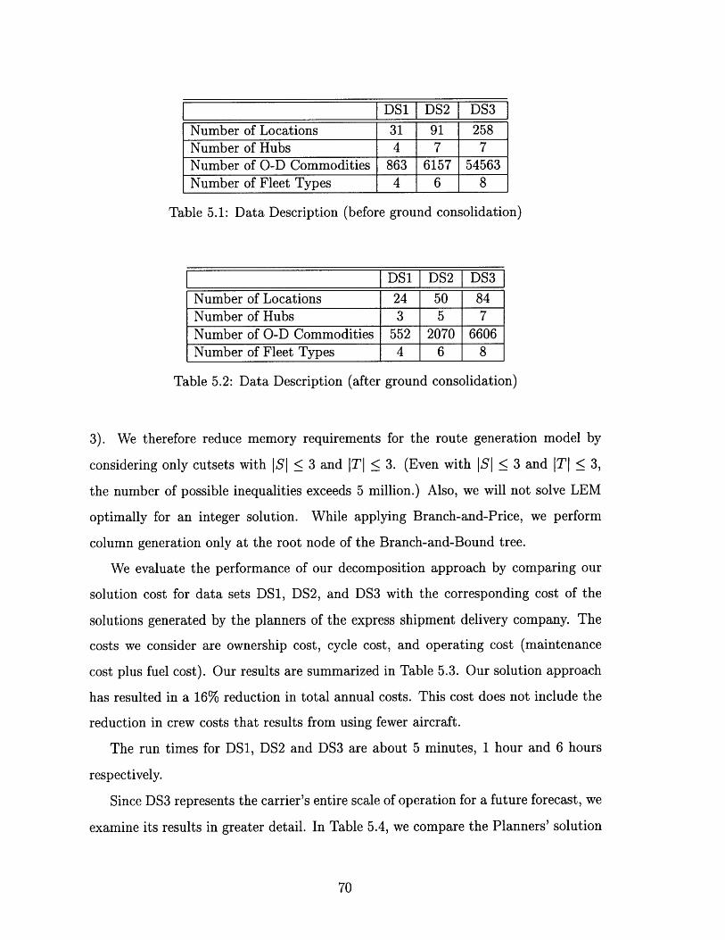
DS1 DS2 DS3Number of Locations 31 91 258Number of Hubs 4 7 7Number of O-D Commodities 863 6157 54563Number of Fleet Types 4 6 8
Table 5.1: Data Description (before ground consolidation)
DS1 DS2 DS3
Number of Locations 24 50 84Number of Hubs 3 5 7Number of O-D Commodities 552 2070 6606Number of Fleet Types 4 6 8
Table 5.2: Data Description (after ground consolidation)
3). We therefore reduce memory requirements for the route generation model by
considering only cutsets with ISI 5 3 and ITI 3. (Even with |SI 3 and ITI 3,
the number of possible inequalities exceeds 5 million.) Also, we will not solve LEM
optimally for an integer solution. While applying Branch-and-Price, we perform
column generation only at the root node of the Branch-and-Bound tree.
We evaluate the performance of our decomposition approach by comparing our
solution cost for data sets DS1, DS2, and DS3 with the corresponding cost of the
solutions generated by the planners of the express shipment delivery company. The
costs we consider are ownership cost, cycle cost, and operating cost (maintenance
cost plus fuel cost). Our results are summarized in Table 5.3. Our solution approach
has resulted in a 16% reduction in total annual costs. This cost does not include the
reduction in crew costs that results from using fewer aircraft.
The run times for DS1, DS2 and DS3 are about 5 minutes, 1 hour and 6 hours
respectively.
Since DS3 represents the carrier's entire scale of operation for a future forecast, we
examine its results in greater detail. In Table 5.4, we compare the Planners' solution
with our solution, contrasting the number of legs flown by aircraft, distance traveled
and aircraft utilization. The comparison of individual cost components, distance,
number of legs, and the number of aircraft for each fleet type is given in Table 5.5.
The figures corresponding to the Planners' solution are given in parentheses. From
these results, we observe the following:
* When compared to the Planners' solution, our solution uses more legs. However,
fewer aircraft are used resulting in a considerable reduction in aircraft ownership
costs that more than offset the increase in the leg-based cycle costs. The reason
we have fewer aircraft is that in our solution, aircraft do a lot of double stopping
because the model has intelligently identified two-legged routes that satisfy LOS
requirements.
* Our solution utilizes cheaper fleet types more effectively. That is, cheaper fleet
types, especially type 4, fly more legs and a longer distance. In our solution,
aircraft of type 4 fly 231 legs and 98,481 miles whereas, in the Planners' solution,
they fly only 165 legs and 76,277 miles. Our solution, with more legs per aircraft
on average, results in a higher utilization of aircraft capacity. The capacity
utilization for our solution is about 66%, compared to 58% for the Planners'
solution.
* In our solution, aircraft do not always trace back their pickup routes on the
delivery side, unlike the Planners' solution. The possible reason for this is
that the shipment demand originating at any gateway location need not be
proportional to that destined for that location and sometimes it is more cost-
effective to use different routes for pickup and delivery. Consider the following
example in which there are two types of aircraft, the first with 200 units of
capacity and the second with 100 units. Supposing we have two locations (1
and 2) with 50 units of demand to be sent from 1 to 2 and 130 units of demand to
be sent from 2 to 1. If the aircraft trace back their pickup routes on the delivery
side, in the best solution, the first aircraft would travel four legs: location 1 to
location 2, location 2 to hub, hub to location 2, and location 2 to location 1.
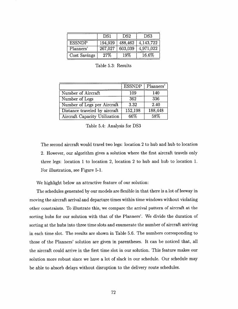
DS1 DS2 DS3
ESSNDP 194,929 488,462 4,143,722Planners' 267,027 603,039 4,971,022
Cost Savings 27% 19% 16.6%
Table 5.3: Results
ESSNDP Planners'
Number of Aircraft 109 140Number of Legs 362 336Number of Legs per Aircraft 3.32 2.40Distance traveled by aircraft 152,198 188,448Aircraft Capacity Utilization 66% 58%
Table 5.4: Analysis for DS3
The second aircraft would travel two legs: location 2 to hub and hub to location
2. However, our algorithm gives a solution where the first aircraft travels only
three legs: location 1 to location 2, location 2 to hub and hub to location 1.
For illustration, see Figure 5-1.
We highlight below an attractive feature of our solution:
The schedules generated by our models are flexible in that there is a lot of leeway in
moving the aircraft arrival and departure times within time windows without violating
other constraints. To illustrate this, we compare the arrival pattern of aircraft at the
sorting hubs for our solution with that of the Planners'. We divide the duration of
sorting at the hubs into three time slots and enumerate the number of aircraft arriving
in each time slot. The results are shown in Table 5.6. The numbers corresponding to
those of the Planners' solution are given in parentheses. It can be noticed that, all
the aircraft could arrive in the first time slot in our solution. This feature makes our
solution more robust since we have a lot of slack in our schedule. Our schedule may
be able to absorb delays without disruption to the delivery route schedules.
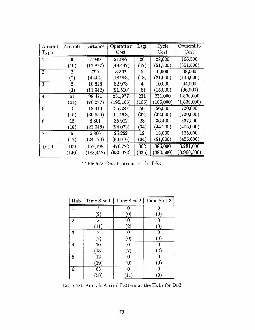
Aircraft Aircraft Distance Operating Legs Cycle OwnershipType Cost Cost Cost
1 9 7,949 21,987 26 28,600 166,500(19) (17,877) (49,447) (47) (51,700) (351,500)
2 2 790 3,362 5 6,000 38,000(7) (4,454) (18,953) (18) (21,600) (133,000)
3 2 10,828 82,973 4 10,000 64,000(3) (11,942) (91,510) (6) (15,000) (96,000)
4 61 98,481 251,977 231 231,000 1,830,000(61) (76,277) (195,165) (165) (165,000) (1,830,000)
5 15 18,443 55,329 56 56,000 720,000(15) (30,656) (91,968) (32) (32,000) (720,000)
6 15 8,801 35,922 28 36,400 337,500(18) (23,048) (94,073) (34) (44,200) (405,000)
7 5 6,866 25,222 12 18,000 125,000(17) (24,194) (88,876) (34) (51,000) (425,000)
Total 109 152,198 476,722 362 386,000 3,281,000(140) (188,448) (630,022) (336) (380,500) (3,960,500)
Table 5.5: Cost Distribution for DS3
Hub Time Slot 1 Time Slot 2 Time Slot 3
1 7 0 0
(9) (0) (0)2 8 0 0
(11) (2) (0)3 7 0 0
(9) (0) (0)4 10 0 0
(13) (7) (2)5 12 0 0
(19) (0) (0)6 63 0 0
(58) (11) (0)
Table 5.6: Aircraft Arrival Pattern at the Hubs for DS3
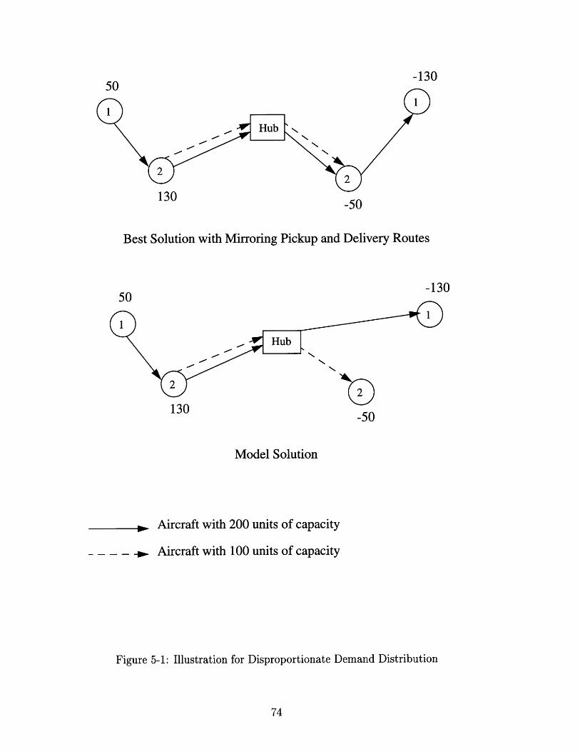
-13050
130 -50
Best Solution with Mirroring Pickup and Delivery Routes
-13050
-50-50
130
Model Solution
Aircraft with 200 units of capacity
S- - - . Aircraft with 100 units of capacity
Figure 5-1: Illustration for Disproportionate Demand Distribution
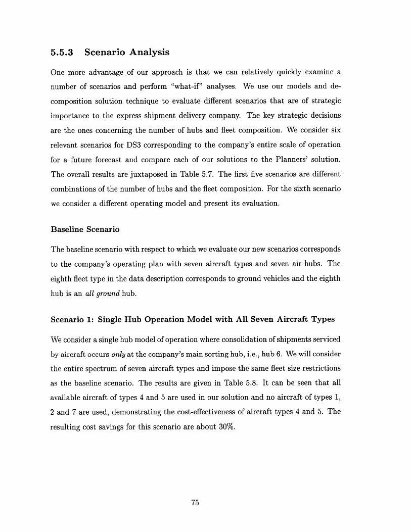
5.5.3 Scenario Analysis
One more advantage of our approach is that we can relatively quickly examine a
number of scenarios and perform "what-if" analyses. We use our models and de-
composition solution technique to evaluate different scenarios that are of strategic
importance to the express shipment delivery company. The key strategic decisions
are the ones concerning the number of hubs and fleet composition. We consider six
relevant scenarios for DS3 corresponding to the company's entire scale of operation
for a future forecast and compare each of our solutions to the Planners' solution.
The overall results are juxtaposed in Table 5.7. The first five scenarios are different
combinations of the number of hubs and the fleet composition. For the sixth scenario
we consider a different operating model and present its evaluation.
Baseline Scenario
The baseline scenario with respect to which we evaluate our new scenarios corresponds
to the company's operating plan with seven aircraft types and seven air hubs. The
eighth fleet type in the data description corresponds to ground vehicles and the eighth
hub is an all ground hub.
Scenario 1: Single Hub Operation Model with All Seven Aircraft Types
We consider a single hub model of operation where consolidation of shipments serviced
by aircraft occurs only at the company's main sorting hub, i.e., hub 6. We will consider
the entire spectrum of seven aircraft types and impose the same fleet size restrictions
as the baseline scenario. The results are given in Table 5.8. It can be seen that all
available aircraft of types 4 and 5 are used in our solution and no aircraft of types 1,
2 and 7 are used, demonstrating the cost-effectiveness of aircraft types 4 and 5. The
resulting cost savings for this scenario are about 30%.
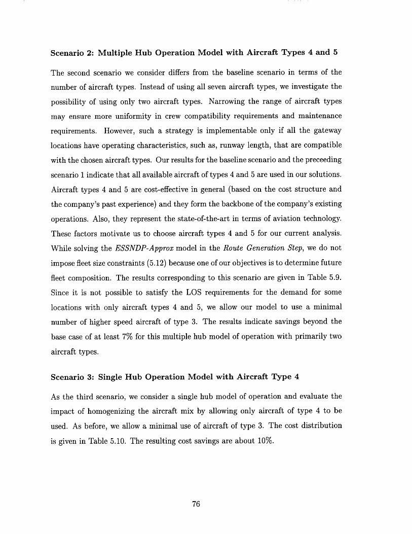
Scenario 2: Multiple Hub Operation Model with Aircraft Types 4 and 5
The second scenario we consider differs from the baseline scenario in terms of the
number of aircraft types. Instead of using all seven aircraft types, we investigate the
possibility of using only two aircraft types. Narrowing the range of aircraft types
may ensure more uniformity in crew compatibility requirements and maintenance
requirements. However, such a strategy is implementable only if all the gateway
locations have operating characteristics, such as, runway length, that are compatible
with the chosen aircraft types. Our results for the baseline scenario and the preceeding
scenario 1 indicate that all available aircraft of types 4 and 5 are used in our solutions.
Aircraft types 4 and 5 are cost-effective in general (based on the cost structure and
the company's past experience) and they form the backbone of the company's existing
operations. Also, they represent the state-of-the-art in terms of aviation technology.
These factors motivate us to choose aircraft types 4 and 5 for our current analysis.
While solving the ESSNDP-Approx model in the Route Generation Step, we do not
impose fleet size constraints (5.12) because one of our objectives is to determine future
fleet composition. The results corresponding to this scenario are given in Table 5.9.
Since it is not possible to satisfy the LOS requirements for the demand for some
locations with only aircraft types 4 and 5, we allow our model to use a minimal
number of higher speed aircraft of type 3. The results indicate savings beyond the
base case of at least 7% for this multiple hub model of operation with primarily two
aircraft types.
Scenario 3: Single Hub Operation Model with Aircraft Type 4
As the third scenario, we consider a single hub model of operation and evaluate the
impact of homogenizing the aircraft mix by allowing only aircraft of type 4 to be
used. As before, we allow a minimal use of aircraft of type 3. The cost distribution
is given in Table 5.10. The resulting cost savings are about 10%.

Scenario 4: Single Hub Operation Model with Aircraft Type 5
The fourth scenario is similar to the third except that we allow the use of aircraft
of type 5 instead of type 4. The cost distribution for this scenario is given in Table
5.11. The resulting cost savings are about 20%. The savings resulting from the use
of only type 5 aircraft are about twice as much as those resulting from the use of
only type 4 aircraft. A possible explanation based on the fact that aircraft of type 5
have a higher capacity than those of type 4, is that there are significant economies
of scale resulting from the use of aircraft of type 5. The total distance traveled, the
total number of legs, and the total number of aircraft are all less when compared
to Scenario 3 resulting in an overall reduction in costs. This is because the total
capacity of aircraft in our solution is 1,012,516 units which is less when compared to
1,041,404 units of capacity for Scenario 3 implying a lesser degree of unused capacity
in the system. Also, the average number of legs per aircraft is higher resulting in an
effective use of two leg routes. For type 5 aircraft, it is possible to have more legs
per aircraft and yet satisfy LOS requirements because, they have higher speed when
compared to type 4 aircraft.
Scenario 5: Single Hub Operation Model with Aircraft Types 4 and 5
We consider a single hub operating model as in the two preceeding scenarios. However,
instead of homogenizing the aircraft mix, we allow the use of two aircraft types
(types 4 and 5). The results for this strategy are shown in Table 5.12. We can
see that for the single hub modus operandi, the strategy allowing the use of both
type 4 and type 5 aircraft is more economical. The reason for this phenomenon
is that the distribution of demand between locations is not uniform and hence two
different aircraft capacities are more effectively used to accomodate these differences
in demand. The total distance traveled, the total number of legs, and the total
number of aircraft are all less when compared to Scenario 3 but they are more when
compared to Scenario 4. The average number of legs per aircraft is greater than that
for Scenario 3 but less than that for Scenario 4. This is because the average aircraft
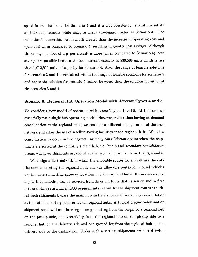
speed is less than that for Scenario 4 and it is not possible for aircraft to satisfy
all LOS requirements while using as many two-legged routes as Scenario 4. The
reduction in ownership cost is much greater than the increase in operating cost and
cycle cost when compared to Scenario 4, resulting in greater cost savings. Although
the average number of legs per aircraft is more (when compared to Scenario 4), cost
savings are possible because the total aircraft capacity is 886,500 units which is less
than 1,012,516 units of capacity for Scenario 4. Also, the range of feasible solutions
for scenarios 3 and 4 is contained within the range of feasible solutions for scenario 5
and hence the solution for scenario 5 cannot be worse than the solution for either of
the scenarios 3 and 4.
Scenario 6: Regional Hub Operation Model with Aircraft Types 4 and 5
We consider a new model of operation with aircraft types 4 and 5. At the core, we
essentially use a single hub operating model. However, rather than having no demand
consolidation at the regional hubs, we consider a different configuration of the fleet
network and allow the use of satellite sorting facilities at the regional hubs. We allow
consolidation to occur in two degrees: primary consolidation occurs when the ship-
ments are sorted at the company's main hub, i.e., hub 6 and secondary consolidation
occurs whenever shipments are sorted at the regional hubs, i.e., hubs 1, 2, 3, 4 and 5.
We design a fleet network in which the allowable routes for aircraft are the only
the ones connecting the regional hubs and the allowable routes for ground vehicles
are the ones connecting gateway locations and the regional hubs. If the demand for
any O-D commodity can be serviced from its origin to its destination on such a fleet
network while satisfying all LOS requirements, we will fix the shipment routes as such.
All such shipments bypass the main hub and are subject to secondary consolidation
at the satellite sorting facilities at the regional hubs. A typical origin-to-destination
shipment route will use three legs: one ground leg from the origin to a regional hub
on the pickup side, one aircraft leg from the regional hub on the pickup side to a
regional hub on the delivery side and one ground leg from the regional hub on the
delivery side to the destination. Under such a setting, shipments are sorted twice,

once at each regional hub.
We first heuristically design the fleet network described above and fix some of the
shipment flows. Then, we use our decomposition approach to design the network for
the shipment demand remaining to be serviced. The cost figures for this new modus
operandi are given in Table 5.13. We see that the cost savings are about 45% more
than the best single hub model as in scenario 5.
Summary
We summarize below the results of our scenario analyses:
* In general, a single hub model of operation is more cost-effective than a mul-
tiple hub model because maximum possible degree of demand consolidation is
attained. The savings from using a single hub model of operation are enhanced
if a new model consisting of main hub consolidation and regional hub consoli-
dation is adopted.
* Aircraft types 4 and 5 are indeed cost-effective. This inference follows from
the fact that all available aircraft of these two types are used by our solutions
in both the baseline scenario corresponding to a multiple hub model and the
second scenario corresponding to a single hub model.
* For the single hub model, using a heterogeneous aircraft mix with two types
(with different capacities) is less expensive than using a homogeneous aircraft
mix because the service network can be more effectively tailored to account for
non-uniform distribution of demand between locations.
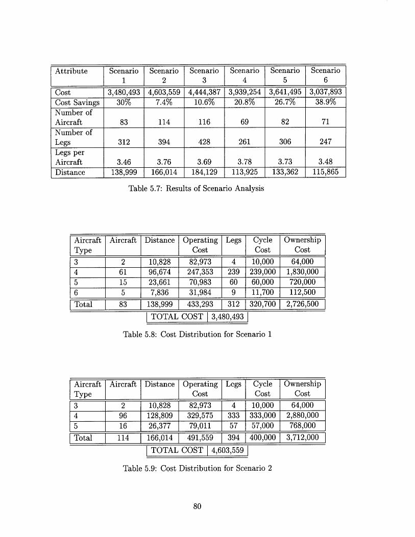
Attribute Scenario Scenario Scenario Scenario Scenario Scenario1 2 3 4 5 6
Cost 3,480,493 4,603,559 4,444,387 3,939,254 3,641,495 3,037,893Cost Savings 30% 7.4% 10.6% 20.8% 26.7% 38.9%Number ofAircraft 83 114 116 69 82 71Number ofLegs 312 394 428 261 306 247Legs perAircraft 3.46 3.76 3.69 3.78 3.73 3.48Distance 138,999 166,014 184,129 113,925 133,362 115,865
Table 5.7: Results of Scenario Analysis
Aircraft Aircraft Distance Operating Legs Cycle OwnershipType Cost Cost Cost
3 2 10,828 82,973 4 10,000 64,0004 61 96,674 247,353 239 239,000 1,830,0005 15 23,661 70,983 60 60,000 720,0006 5 7,836 31,984 9 11,700 112,500
Total 83 138,999 433,293 312 320,700 2,726,500
TOTAL COST 3,480,493
Table 5.8: Cost Distribution for Scenario 1
Aircraft Aircraft Distance Operating Legs Cycle OwnershipType Cost Cost Cost
3 2 10,828 82,973 4 10,000 64,0004 96 128,809 329,575 333 333,000 2,880,0005 16 26,377 79,011 57 57,000 768,000
Total 114 166,014 491,559 394 400,000 3,712,000
TOTAL COST 4,603,559
Table 5.9: Cost Distribution for Scenario 2
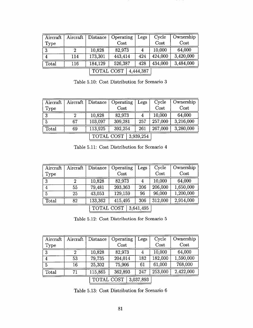
Aircraft Aircraft Distance Operating Legs Cycle OwnershipType Cost Cost Cost
3 2 10,828 82,973 4 10,000 64,0004 114 173,301 443,414 424 424,000 3,420,000
Total 116 184,129 526,387 428 434,000 3,484,000
TOTAL COST 4,444,387
Table 5.10: Cost Distribution for Scenario 3
Aircraft Aircraft Distance Operating Legs Cycle OwnershipType Cost Cost Cost
3 2 10,828 82,973 4 10,000 64,0005 67 103,097 309,281 257 257,000 3,216,000
Total 69 113,925 392,254 261 267,000 3,280,000
TOTAL COST 3,939,254
Table 5.11: Cost Distribution for Scenario 4
Aircraft Aircraft Distance Operating Legs Cycle OwnershipType Cost Cost Cost
3 2 10,828 82,973 4 10,000 64,0004 55 79,481 203,363 206 206,000 1,650,0005 25 43,053 129,159 96 96,000 1,200,000
Total 82 133,362 415,495 306 312,000 2,914,000
TOTAL COST 3,641,4951
Table 5.12: Cost Distribution for Scenario 5
Aircraft Aircraft Distance Operating Legs Cycle OwnershipType Cost Cost Cost
3 2 10,828 82,973 4 10,000 64,0004 53 79,735 204,014 182 182,000 1,590,0005 16 25,302 75,906 61 61,000 768,000
Total 71 115,865 362,893 247 253,000 2,422,000
TOTAL COST 3,037,893 1
Table 5.13: Cost Distribution for Scenario 6

Chapter 6
Closure
6.1 Conclusions
In this thesis, we present an iterative modeling framework and a decomposition so-
lution algorithm for large scale transportation service network design problems with
time windows. We provide a proof-of-concept of the efficacy of our solution approach
by solving the service network design problem of a large carrier in the express ship-
ment delivery industry.
6.2 Future Research Directions
We present below some directions for future research:
* The immediate task is to evaluate more thoroughly the solutions generated by
our models and arrive at a better quantification of the benefits. For instance,
in our express shipment delivery application we did not measure the savings in
crew costs resulting from our solution.
* The models we have developed are deterministic in nature and assume a con-
stant market demand. However, the demand varies cyclically with the day of
the week as well as stochastically. There is a need to test the robustness of our
solution with respect to changing demand patterns. The usage of our models
and algorithms within a stochastic optimization framework should be explored
to consider variations in demand.
* We need to develop efficient branching strategies for use within a Branch-and-
Price-and-Cut solution framework for the Route Generation problem.
* Finding an efficient, or an approximate, algorithm for the cutset separation
problem would lessen the computational burden of solving the Route Generation
problem.
* While there exist approximation algorithms for telecommunication network de-
sign, approximation schemes that exploit the hub-and-spoke structure of trans-
portation service network design problems need to be developed so that feasible
integer solutions with theoretically known bounds can be achieved.
* From an applied perspective, we need to enhance our models to consider service
differentiation. For the express shipment delivery application, we need to plan
for different levels of service such as the Next Day Service, Second Day Service,
Deferred Service and so on.
Appendix A
Notations
A.1 SETS
N(3 i) : the set of all nodes in the service network
A(3 (i, j)) : the set of all arcs in the service network
G = (N, A) : the service network with set of nodes N and set of arcs A
K(3 k) : the set of all O-D commodities
F(3 f) : the set all asset types available
Rf (3 r) : the set of all design routes for fleet type f
Rf (3 r):the set of all design pickup routes for fleet type f
Rf (9 r):the set of all design delivery routes for fleet type f
pk( 3 p) : the set of all feasible paths from origin O(k) to destination D(k) for eack
keK
0(3 o) : set of all origin locations
D(3 d) : set of all destination locations
Qo (3 q) : the set of all trees at origin o, for all o E 0
Ko : the set of all O-D commodities with origin o
Kd : the set of all O-D commodities with destination d
Od : the set of all origins o such that there exists a commodity with O(k) = o and
D(k) = d, for each d E D
Do : the set of all destinations d such that there exists a commodity with O(k) = o
and D(k) = d, for each o E O
pk : the unique path from O(k) to D(k) in tree q
A.2 PARAMETERS
bk : the demand for commodity for each k E K
uij : the capacity of arc (i, j) E A
hf = E(i,j)EA hij j: the cost of design route r of type f
c = E(i,j)EA cjfj : the cost of flowing one unit of commodity k from O(k) to D(k)
along path p E pk
cq = EkgEKo Z(i,j)EA Ikk : the cost of flowing the entire portion of all O-D commodi-
ties with O(k) = o from O(k) to D(k) along path pk in tree q.
A.3 INDICATOR VARIABLES
1 if arc (i, j) belongs to the path pk from 0(k) to D(k) in tree q
0 otherwise
1 if design variable for (i, j) is included in design route r0 otherwise
1
# = -1
if i E N is the start node of design route r
if i E N is the end node of design route r
otherwise
if arc (i, j) belongs to path p
otherwise
A.4 DECISION VARIABLES
yf : number of assets of type f deployed on design route r
x : fraction of bk on path p E Pk for all k E K
wq: fraction of bk flown on the path pk from O(k) = o to D(k) in tree q
{ 1 if if all the O-D commodities with O(k) = o are assigned to network paths
0 otherwise
Zd= {0
if if all the O-D commodities with D(k) = d are assigned to network paths
otherwise
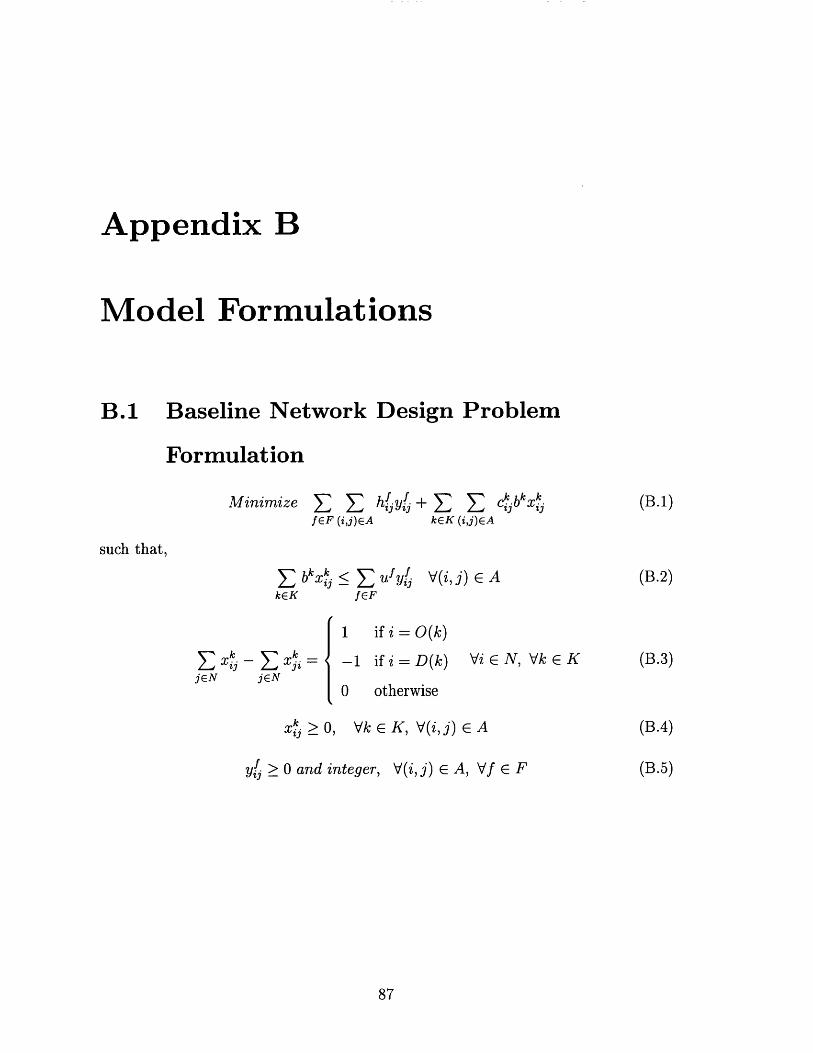
Appendix B
Model Formulations
B.1 Baseline Network Design Problem
Formulation
Minimize j y + k ckb k.
ffEE (i,j)EA keK (i,j)EA
such that,
bk kX
kEKfE ufyfEF
V(i, j) E A
1 if i = O(k)
-1 if i= D(k)
0 otherwisejEN
Vi E N, Vk E K
xijk >, Vk E K, V(i,j) E A
y41 > 0 and integer,
(B.1)
jEjeN
(B.2)
(B.3)
(B.4)
(B.5)V(i,j) E A, Vf E F
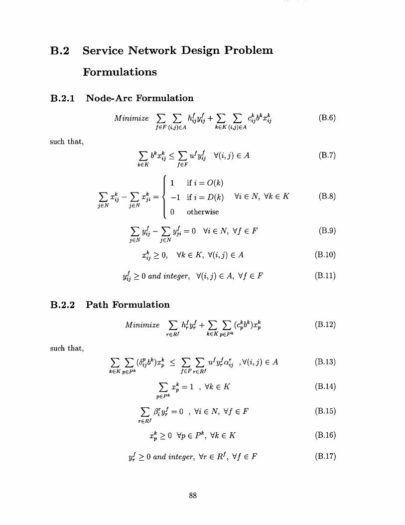
B.2 Service Network Design Problem
Formulations
B.2.1 Node-Arc Formulation
Minimize EfEF
such that,
E bkkEK
(i,j)EA
f EF
.C k bk k~+ E cijb ijkeK (i,j)EA
V(i,j) e A
if i = O(k)
if i = D(k)
otherwise
Vi E N, Vk E K
Vi E N, Vf E F
x > 0,X3
y2 > 0 and integer,
Vk e K, V(i,j) E A
V(i,j) E A, Vf E F
B.2.2 Path Formulation
Minimize E hyf + C (ckbk)zrERf kEKpEPk
such that,
fEF rERf
, V(i, j) E A
x 2 1 , Vk e KpEpk
Py r= 0 , Vi E N, V f E FrERf
xk 0 Vp E P k , Vk E K
yf > 0 and integer, Vr E RI , Vf E F
(B.6)
xjNjEN
1
- -1
0
- ENjEN
(B.7)
jENjEN
(B.8)
-ENf =jEN
(B.9)
(B.10)
(B.11)
EE p bk <
kEK pEP k
(B.12)
(B.13)
(B.14)
(B.15)
(B.16)
(B.17)
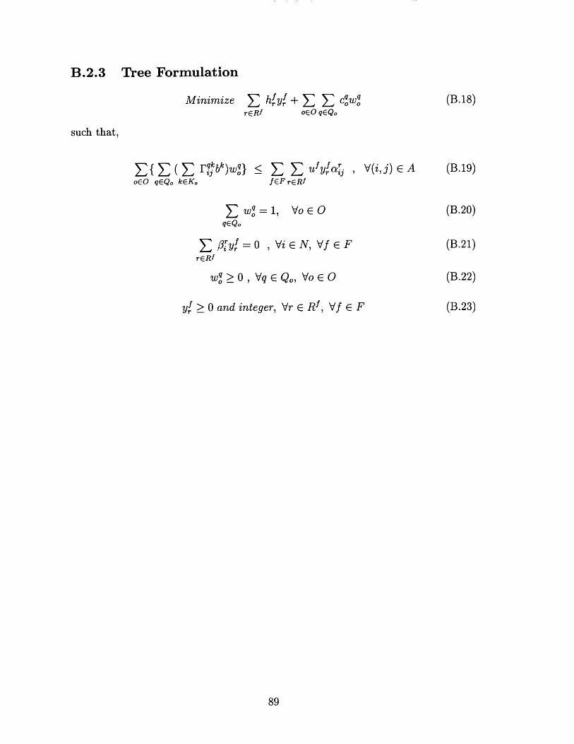
B.2.3 Tree Formulation
Minimize ErERf
hf Yl + EE q C q
oEO qEQo
f< E uryERffEF rERf
wg = 1, Vo E OqEQo
O ry = 0 , Vi E N, Vf E FrERI
w , Vq e Qo, Vo E O
y/ _ 0 and integer, Vr E R f , Vf E F
such that,
(B.18)
E{ ( E Q bkK,oCO qCQo keKo
, V(i,j) E A (B.19)
(B.20)
(B.21)
(B.22)
(B.23)

B.3 The Approximate Service Network Design
Cutset Model
B.3.1 Node-Arc Formulation
(B.24)Minimize y hyfEF (i,j)EA
such that
E UfYSf, T DS,T ,fef
y! - E y =jEN jEN
yt 2> 0 and integer,
S0 - D cutsets {S, T}
0 Vi E N, Vf E F
V(i,j) E A, Vf e F
E Uf YST DS,TfEf
Pry f = 0rERI
SV 0- D cutsets {S, T}
, Vi N, Vf F
(B.25)
(B.26)
(B.27)
B.3.2 Route Formulation
such that
Minimize hf yfrERf
(B.28)
y 0 and integer, Vr E R f , Vf E F
(B.29)
(B.30)
(B.31)
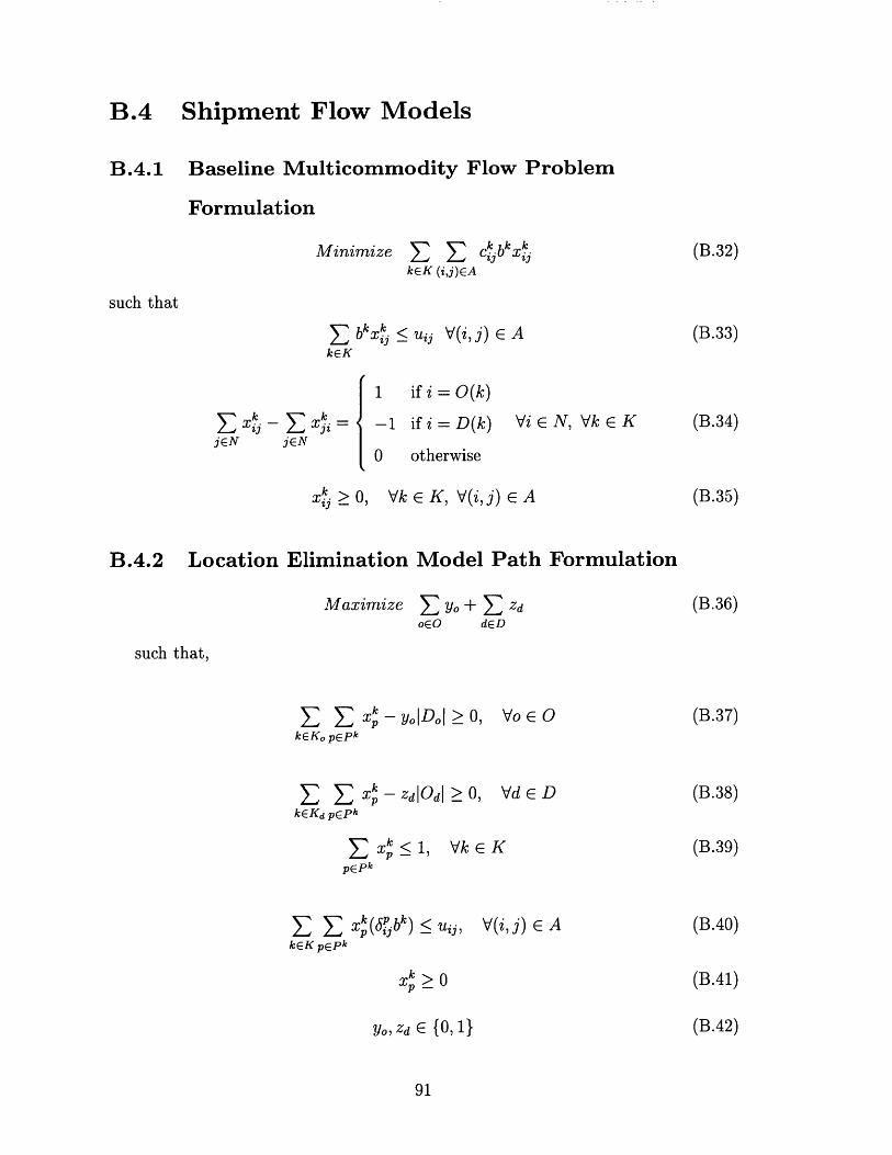
B.4 Shipment Flow Models
B.4.1 Baseline Multicommodity Flow Problem
Formulation
(B.32)Minimize c kk 2kEK (i,j)EA
Sbkx < uij V(i,j) E AkEK
(B.33)
if i = O(k)
1 if i= D(k)
otherwise
Vi e N, Vk E K
xi >O, Vk E K, V(i,j) E A
B.4.2 Location Elimination Model Path Formulation
Maximize Z Yo + Z ZdoEO dED
xp - yolDol > 0,kEKo pEPk
x - zdjOd > 0,kEKd pEPk
p k < 1,pEpk
X b(6jb k) _ ui,kEK pEPk
S1>O
yo, zd E {0, 1}
V(i,j) E A
such that
1
0jEN jEN
(B.34)
(B.35)
such that,
(B.36)
Vo E O
Vd E D
(B.37)
(B.38)
(B.39)Vk E K
(B.40)
(B.41)
(B.42)
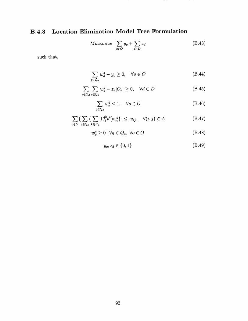
B.4.3 Location Elimination Model Tree Formulation
Maximize 1 yo + E Zd (B.43)oEO dED
such that,
Swq - yo > O, Vo ( O (B.44)qEQo
S w q - ZdiOdl O, Vd ED (B.45)oEOd qCQo
wq < 1 Vo GO (B.46)qEQo
{ ( L ~bk)wq} uij, V(i,j) c A (B.47)oEO qEQo kEKo
w > O, VqE Qo, Vo E O (B.48)
Yo, Zd E {0, 1} (B.49)
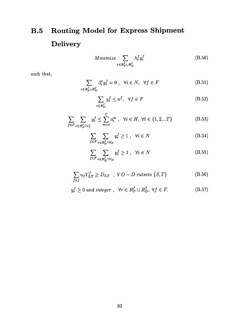
B.5 Routing Model for Express Shipment
Delivery
(B.50)Minimize ZreRfURfP D
ViEN, Vf cF~Ryf =0 ,
P D
SYf nf, Vf E F
T
< y E am , ViEH, VtE(1,2,..T}
Zy Z y>I, Vi ENfEF rER, nVp
S 1yf > Vi ENfcF rER nVD
SUf YIT > DS,T , V 0 - D cutsets {S, T}f1f
Vr Rf U Rf, Vf E F.yrf > 0 and integer ,
such that,
(B.51)
(B.52)
(B.53)
(B.54)
(B.55)
(B.56)
(B.57)
h yfr gr

References
[1] J. Abara. Applying integer linear programming to the fleet assignment problem.
Interfaces, 19, 1989.
[2] A. Agrawal, P. Klein, and R. Ravi. When trees collide: An approximation
algorithm for the generalized steiner problem on networks. SIAM Journal on
Computing, 24, 1995.
[3] R.K. Ahuja, T.L. Magnanti, and J.B. Orlin. Network Flows: Theory, Algorithms
and Applications. Prentice Hall, 1993.
[4] R. Anbil, E. Gelman, B. Petty, and R. Tanga. Recent advances in crew-pairing
optimization at American Airlines. Interfaces, 21(1), 1991.
[5] A. Balakrishnan, T.L. Magnanti, and P. Mirchandani. A Dual-Based Algorithm
for Multi-level Network Design. Managament Science, 40(5), 1994.
[6] A. Balakrishnan, T.L. Magnanti, and P. Mirchandani. Modeling and Heuris-
tic Worst-case Performance Analysis of the Two-level Network Design Problem.
Management Science, 40(7), 1994.
[7] A. Balakrishnan, T.L. Magnanti, and P. Mirchandani. Heuristics, LPs, and Trees
on Trees: Network Design Analyses. Operations Research, 44(3), 1996.
[8] A. Balakrishnan, T.L. Magnanti, and R. T. Wong. A Decomposition Algorithm
for Local Access Telecommunications Network Expansion Planning. Operations
Research, 43(1), 1995.
[9] D. Barnett, J. Binkley, and B McCarl. The effects of U.S. port capacity con-
straints on national and world grain shipments. Technical paper, Purdue Uni-
versity, 1982.
[10] C. Barnhart. Dual-Ascent Methods for Large-Scale Multicommodity Flow Prob-
lems. Naval Research Logistics, 40, 1993.
[11] C. Barnhart, N. L. Boland, L. W. Clarke, E. L. Johnson, G. L. Nemhauser, and
R. G. Shenoi. Flight String Models for Aircraft Fleeting and Routing. Trans-
portation Science. To appear.
[12] C. Barnhart, C.A.Hane, and P.H.Vance. Integer Multicommodity Flow Prob-
lems. Operations Research. To appear.
[13] C. Barnhart, C. A. Hane, E. L. Johnson, and G. Sigismondi. A Column Gener-
ation and Partitioning Approach for Multicommodity Flow Problems. Telecom-
munication Systems, 3, 1995.
[14] C. Barnhart, H. Jin, and P. H. Vance. Railroad Blocking: A Network Design
Application. Working paper, Center for Transportation Studies, MIT, 1997.
[15] C. Barnhart, E. L. Johnson, R. Anbil, and L. Hatay. A Column Generation
Technique for the Long-Haul Crew-Assignment Problem. In T. A. Ciriani and
R. C. Leachman, editors, Optimization in Industry, volume 2. 1991.
[16] C. Barnhart, E. L. Johnson, G. L. Nemhauser, M. W. F. Salvelsbergh, and
P. H. Vance. Branch-and-Price: Column Generation for Solving Huge Integer
Programs. Operations Research. To appear.
[17] C. Barnhart, F. Lu, and R. Shenoi. Integrated Airline Scheduling, volume 9
of Operations Research in the Air Industry, International Series in Operations
Research in Management Science. Kluwer Academic Publishers, 1997.
[18] C. Barnhart and R.R. Schneur. Air Network Design for Express Shipment Ser-
vice. Operations Research, 44(6), 1996.
[19] C. Barnhart and Y. Sheffi. A Network Based Primal-Dual Heuristic for the
Solution of Multicommodity Network Flow Problems. Transportation Science,
27(2), 1993.
[20] S. P. Bradley, A. C. Hax, and T. L. Magnanti. Applied Mathematical Program-
ming. Addison-Wesley Publishing Company, 1977.
[21] Y. Chan and R. J. Ponder. The Small Package Air Freight Industry in the United
States: A Review of the Federal Express Experience. Transportation Research -
A, 13A, 1979.
[22] L. Chestler. Overnight Air Express: Spatial Pattern, Competition and the Future
in Small Package Delivery Services. Transportation Quarterly, 39(1), 1985.
[23] L. W. Clarke, E. L. Johnson, G. L. Nemhauser, and Z. Zhu. The aircraft rotation
problem. Annals of OR: Mathematics of Industrial Systems, 2. To appear.
[24] L. W. Clarke and Gong. P. Capacitated network design with column generation.
LEC-96-06, Report Series Librarian, The Logistics Institute, Research Division,
School of Industrial and Systems Engineering, Georgia Institute of Technology,
1995.
[25] T. H. Cormen, C. L. Leiserson, and R. L. Rivest. Introduction to Algorithms.
MIT Press and McGraw Hill, 1990.
[26] CPLEX Optimization Inc. Using the CPLEX Callable Library, version 4.0.
CPLEX Optimization, Inc., 1995.
[27] T. Crainic, J. A. Ferland, and J. M. Rousseau. A tactical planning model for
Rail freight transportation. Transportation Science, 18, 1984.
[28] G. B. Dantzig and P. Wolfe. Decomposition Principle for Linear programs. Op-
erations Research, 8, 1960.
[29] M. S. Daskin and N. D. Panayotopoulos. A Lagrangian Relaxation Approach
to Assigning Aircraft to Routes in Hub and Spoke Networks. Transportation
Science, 23(2), 1989.
[30] G. Desauliniers, J. Desrosiers, I. Ioachim, M. Solomon, and F. Soumis. A unified
framework for deterministic time constrained vehicle routing and crew scheduling
problems. Working Paper, GERAD, 1994.
[31] M. Desrochers and F. Soumis. A Column Generation Approach to the Urban
Transit Crew Scheduling Problem. Transportation Science, 23, 1989.
[32] J. Desrosiers, Y. Dumas, M. Solomon, and F. Soumis. Time Constrained Routing
and Scheduling. North Holland. To appear.
[33] J. M. Farvolden and W. B. Powell. Subgradient Methods for the Service Network
Design Problem. Transportation Science, 28(4), 1986.
[34] J. M. Farvolden, W. B. Powell, and I. J. Lustig. A Primal Partitioning Solution
for the Arc-Chain Formulation of a Multicommodity Network Flow Problem.
Operations Research, 4(4), 1993.
[35] T. A. Feo and J. F. Bard. Flight scheduling and maintenence base planning.
Management Science, 35, 1989.
[36] L. R. Foulds. A multicommodity network design problem. Transportation Re-
search(B), 15(4), 1981.
[37] H. N. Gabow, M. X. Goemans, and D. P. Williamson. An efficient approximation
algorithm for the survivable network design problem. In Proc. of the 3rd MPS
Conference on Integer Programming and Combinatorial Optimization, 1993.
[38] B. Gendron and T. G. Crainic. Relaxations for multicommodity capacitated
network design problems. Working Paper, Centre de recherche sur les transports
- Publication #965, Universite de Montreal, 1994.
[39] M. X. Goemans, A. V. Goldberg, S. A. Plotkin, D. B. Shmoys, E. Tardos, and
D. P. Williamson. Improved approximation algorithms for network design prob-
lems. In Proceedings of 5th ACM-SIAM Symposium on Discrete Algorithms,
Arlington, Virginia, 1994.
[40] M. X. Goemans and D. P. Williamson. The Primal-Dual method for approxima-
tion algorithms and its application to network design problems. In Hochbaum,
editor, Approximation Algorithms. To Appear.
[41] M. X. Goemans and D. P. Williamson. A general approximation technique for
constrained forest problems. SIAM Journal on Computing, 24, 1995.
[42] B. L. Golden and A. A. Assad. Vehicle Routing: Methods and Studies. Studies
in Management Science and Systems. North-Holland, 1988.
[43] R. W. Hall. Configuration of an Overnight Package Sir Network. Transportation
Research - A, 23A(2), 1989.
[44] C. A. Hane, C. Barnhart, E. L. Johnson, R. E. Marsten, G. L. Nemhauser,
and G. Sigismondi. The fleet assignment problem: solving a large-scale integer
program. Mathematical Programming, 70, 1995.
[45] R. Helgason, J. Kennington, and P. Wong. An application of network program-
ming for national forest planning. Technical Report OR 81006, Department of
Operations Research, Southern Methodist University, Dallas, 1981.
[46] D. S. Hochbaum and J. S. Naor. Approximation Algorithms for Network Design
Problems on Bounded Subsets. Journal of Algorithms, 21, 1996.
[47] International Business Machines Corp. IBM Optimization Subroutine Library
(OSL) Guide and Reference, volume 31. IBM Systems Journal, SC23-0519, 1992.
[48] K. L. Jones, I. J. Lustig, J. M. Farvolden, and W. B. Powell. Multicommod-
ity network flows: The impact of formulation on decomposition. Mathematical
Programming Study, 26, 1986.
[49] M. Kamoun and R. W. Hall. Design of Express Mail Services for Metropolitan
Regions. Journal of Business Logistics, 17(2), 1996.
[50] A. Kanafani and A. A. Ghobrial. Airline Hubbing - Some Implications for Airport
Economics. Transportation Research - A, 19A(1), 1985.
[51] J. L. Kennington. A Survey of Linear Multicommodity Network Flows. Opera-
tions Research, 26, 1978.
[52] D. Kim. Large Scale Transportation Service Network Design: Models, Algorithms
and Applications. PhD dissertation, Massachusetts Institute of Technology, De-
partment of Civil Engineering, June 1997.
[53] P. Klein, S. Plotkin, C. Stein, and E. Tardos. Faster approximation algorithms
for the unit capacity concurrent flow problem with applications to routing and
sparse cuts. SIAM Journal on Computing, 23, 1994.
[54] M. J. Kuby and R. G. Gray. The Hub Network Design Problem with Stopovers
and Feeders: The Case of Federal Express. Transportation Research - A, 27A(1),
1993.
[55] T. Leighton, F. Makedon, S. Plotkin, C. Stein, E. Tardos, and S. Tragoudas.
Fast approximation algorithms for multicommodity flow problems. Journal of
Computer and System Sciences, 50, 1995.
[56] T. Leighton and S. Rao. An Approximate Max-Flow Min-Cut Theorem for
Uniform Multicommodity Flow Problems with Application to Approximation
Algorithms. In 29th Annual Symposium on Foundations of Computer Science,
1988.
[57] C. Li, S. T. McCormick, and D. Simchi-Levi. The point-to-point delivery and
connection problems: complexity and algorithms. Discrete Applied Mathematics,
36, 1992.
[58] N. Linial, E. London, and Y. Rabinovich. The geometry of graphs and some of its
algorithmic applications. In Proc. of the 35th Annual Symposium on Foundations
of Computer Science, 1994.
[59] T.L. Magnanti. Combinatorial Optimization and Vehicle Fleet Planning: Per-
spectives and Prospects. Networks, 11, 1981.
[60] T.L. Magnanti and P. Mirchandani. Shortest Paths, Single Origin-Destination
Network Design and Associated Polyhedra. Networks, 23, 1993.
[61] T.L. Magnanti, P. Mirchandani, and R. Vachani. The Convex Hull of Two Core
Capacitated Network Design Problems. Mathematical Programming, 60, 1993.
[62] T.L. Magnanti, P. Mirchandani, and R. Vachani. Modeling and Solving the Two-
Facility Capacitated Network Loading Problem. Operations Research, 43(1),
1995.
[63] T.L. Magnanti, P. Mireault, and R.T. Wong. Tailoring Benders Decomposition
for Uncapacitated Network Design Problem. Mathematical Programming Study,
26, 1986.
[64] T.L. Magnanti and R.T. Wong. Network Design and Transportation Planning:
Models and Algorithms. Transportation Science, 18(1), 1984.
[65] D. Medhi and D. Tipper. On some approaches to solving a multi-hour commu-
nication network design problem. Working Paper, Computer Science Telecom-
munications, University of Missouri - Kansas City, 1995.
[66] M. Minoux. Network Synthesis and Optimum Network Design Problems: Mod-
els, Solution Methods and Applications. Network, 19, 1989.
[67] P. Mirchandani. Polyhedral Structure of the Capacitated Network Design Prob-
lem with an Application to the Telecommunication Industry. PhD dissertation,
Massachusetts Institute of Technology, 1989.
100
[68] N. Nabonna. Multicommodity network flow model for long term hydro-
generation optimization. IEEE transactions on power systems, 8, 1993.
[69] G. L. Nemhauser, M. W. P. Salvelsbergh, and G. C. Sigismondi. MINTO, A
Mixed INTeger Optimizer. Operations Research Letters, 15, 1994.
[70] G. L. Nemhauser and L. A. Wolsey. Integer and Combinatorial Optimization.
John Wiley and Sons, Inc., 1988.
[71] H. N. Newton. Network Design Under Budget Constraints with Application to
the Railroad Blocking Problem. PhD dissertation, Auburn University, Alabama,
1996.
[72] M. E. O'Kelly. The Location of Interacting Hub Facilities. Transportation Sci-
ence, 20(2), 1986.
[73] M. Parker and J. Ryan. A column generation algorithm for bandwidth packing.
Telecommunications Systems. To appear.
[74] W. B. Powell. A Local Improvement Heoristic for the Design of Less-than-
Truckload Motor Carrier Networks. Transportation Science, 20(3), 1994.
[75] W. B. Powell and Y. Sheffi. Design and Implementation of an Interactive Opti-
mization System for Network Design in the Motor Carrier Industry. Operations
Research, 39, 1989.
[76] T. Radzik. Fast deterministic approximation for the multicommodity flow prob-
lem. Mathematical Programming, 78(1), 1997.
[77] P. Raghavan and C.D.Thompson. Randomized Rounding: A Technique for
Provably Good Algorithms and Algorithmic Proofs. Combinatorica, 4, 1987.
[78] G. Saviozzi. Advanced Start for the Multicommodity Network Flow Problem.
Mathematical Programming Study, 26, 1986.
101
[79] R. R. Schneur. Scaling Algorithms for Multicommodity Flow Problems and Net-
work Problems with Side Constraints. PhD dissertation, Massachusetts Institute
of Technology, Department of Civil Engineering, June 1991.
[80] G. L. Schultz and R. R. Meyer. An Interior Point Method for Block Angular
Optimization. SIAM Journal on Optimization, 1(4), 1991.
[81] R. S. Segall. Mathematical modeling of spatial price equilibrium for multicom
modity consumer flows of large markets using variational inequalities. Applied
Mathematical Modeling, 9, 1995.
[82] Y. Sheffi. Transportation and Logistics Analysis. MIT Course Notes, 1997.
[83] R. G. Shenoi. Integrated Airline Schedule Optimization: Models and Solution
Methods. PhD dissertation, Massachusetts Institute of Technology, Department
of Civil Engineering, 1996.
[84] M. Stoer. Design of Survivable Networks. Lecture Notes in Mathematics 1531.
Springer-Verlag, 1992.
[85] K. T. Talluri and R. Gopalan. Mathematical Models in Airline Scheduling Plan-
ning: A Survey. Working Paper, USAir, Operations Research Department, Ar-
lington, VA.
[86] P. M. Vaidya. Speeding Up Linear Programming Using Fast Matrix Multiplica-
tion. Proceedings of the 30th Annual Symposium on Foundations of Computer
Science, 1989.
[87] P. H. Vance, C. Barnhart, E. L. Johnson, and G. L. Nemhauser. Solving Bi-
nary Cutting Stock Problems by Column Generation and Branch-and-Bound.
Computational Optimization and Applications. To appear.
[88] D. P. Williamson, M. X. Goemans, M. Mihail, and V. V. Vazirani. A primal-dual
approximation algorithm for generalized Steiner network problems. In Proc. of
the 25th ACM Symposium on Theory of Computing, 1993.
102
[89] R. T. Wong. Transportation and Network Research: Algorithmis and Compu-
tational Questions. Transportation Research - A, 19A(5/6), 1985.
[90] S. A. Zenios. On the Fine-Grain Decomposition of Multicommodity Transporta-
tion Problems. SIAM Journal on Optimization, 1(4), 1991.
[91] K. Ziarati, F. Soumis, J. Desrosiers, S. Gelinas, and A. Saintonge. Locomotive
Assignment with Heterogeneous Consists at CN North America. Working Paper,
GERAD and Ecole Polytechnique de Montreal, 1995.
103