Embed Size (px)
Citation preview

Algorithms for Self-Healing Networks
Trehan, A. (2010, May). Algorithms for Self-Healing Networks. https://arxiv.org/abs/1305.4675
Document Version:Other version
Queen's University Belfast - Research Portal:Link to publication record in Queen's University Belfast Research Portal
Publisher rights© 2010 The Author
General rightsCopyright for the publications made accessible via the Queen's University Belfast Research Portal is retained by the author(s) and / or othercopyright owners and it is a condition of accessing these publications that users recognise and abide by the legal requirements associatedwith these rights.
Take down policyThe Research Portal is Queen's institutional repository that provides access to Queen's research output. Every effort has been made toensure that content in the Research Portal does not infringe any person's rights, or applicable UK laws. If you discover content in theResearch Portal that you believe breaches copyright or violates any law, please contact [email protected].
Download date:14. Dec. 2021

Algorithms for Self-Healing Networks
by
Amitabh Trehan
B.Sc., Biology, Punjab University, 1994
M.C.A., Indira Gandhi National Open University, 2000
M.Tech., Indian Institute of Technology Delhi, 2002
DISSERTATION
Submitted in Partial Fulfillment of the
Requirements for the Degree of
Doctor of Philosophy
Computer Science
The University of New Mexico
Albuquerque, New Mexico
May, 2010
arX
iv:1
305.
4675
v1 [
cs.D
S] 2
0 M
ay 2
013

c©2013, Amitabh Trehan
iii

Dedication
To the sun, the moon
and the intrepid spirit,
To my family
who made this journey possible.
The question walks
the length of pages,
rain drops on roof.
iv

Acknowledgments
If this were an Oscar awards ceremony, my list of thank yous would have had themusic director going crazy trying to hound me off the stage. There are many manyto thank for the journey responsible for this document. My foremost gratitude goestowards my advisor, Professor Jared Saia, for his constant enthusiastic guidance.He has patiently ironed out a multitude of rough edges that I, as a scientist, havepresented, and has taught the virtues of discipline and mathematical rigour. Myacademic collaborator and committee member Professor Thomas Hayes has been asource of constant inspiration. I am thankful to my dissertation committee (Pro-fessors Saia, Hayes, Cris Moore and Tanya-Beger Wolf) who have provided me withmuch insight and guidance. I am thankful to all my close friends, who have beenwith me through good times and bad, especially Navin Rustagi and Vaibhav Mad-hok (their lively discussions have lit up many evenings!). I am thankful to the USeducational system, for its support of quality graduate education and research. I owea debt of gratitude to all my teachers and friends in India, and to the Art of Livingfoundation and it’s founder Sri Sri Ravi Shankar, for Sudershan Kriya, the medita-tion and the satsangs . Finally, I have to thank my biggest inspiration: my mother,and my family: my late father, my step-father, my brothers, my sister-in-laws, mynieces and my nephew, without whose support and love I would never have been ableto pursue the path around the world and in my academic world that I have.
v

Algorithms for Self-Healing Networks
by
Amitabh Trehan
ABSTRACT OF DISSERTATION
Submitted in Partial Fulfillment of the
Requirements for the Degree of
Doctor of Philosophy
Computer Science
The University of New Mexico
Albuquerque, New Mexico
May, 2010

Algorithms for Self-Healing Networks
by
Amitabh Trehan
B.Sc., Biology, Punjab University, 1994
M.C.A., Indira Gandhi National Open University, 2000
M.Tech., Indian Institute of Technology Delhi, 2002
Ph.D., Computer Science, University of New Mexico, 2013
Abstract
Many modern networks are reconfigurable, in the sense that the topology of the
network can be changed by the nodes in the network. For example, peer-to-peer,
wireless and ad-hoc networks are reconfigurable. More generally, many social net-
works, such as a company’s organizational chart; infrastructure networks, such as an
airline’s transportation network; and biological networks, such as the human brain,
are also reconfigurable. Modern reconfigurable networks have a complexity unprece-
dented in the history of engineering, resembling more a dynamic and evolving living
animal rather than a structure of steel designed from a blueprint. Unfortunately, our
mathematical and algorithmic tools have not yet developed enough to handle this
complexity and fully exploit the flexibility of these networks.
We believe that it is no longer possible to build networks that are scalable and
never have node failures. Instead, these networks should be able to admit small, and
vii

maybe, periodic failures and still recover like skin heals from a cut. This process,
where the network can recover itself by maintaining key invariants in response to
attack by a powerful adversary is what we call self-healing.
Here, we present several fast and provably good distributed algorithms for self-
healing in reconfigurable dynamic networks. Each of these algorithms have different
properties, a different set of gaurantees and limitations. We also discuss future
directions and theoretical questions we would like to answer.
viii

Contents
List of Figures xiii
List of Tables xviii
1 Introduction 1
1.1 Naive self-healing . . . . . . . . . . . . . . . . . . . . . . . . . . . . . 4
1.2 Model of self-healing . . . . . . . . . . . . . . . . . . . . . . . . . . . 4
1.3 Healing by Reconstruction Trees . . . . . . . . . . . . . . . . . . . . . 8
1.4 Our Results . . . . . . . . . . . . . . . . . . . . . . . . . . . . . . . . 9
1.5 Related Work . . . . . . . . . . . . . . . . . . . . . . . . . . . . . . . 12
1.5.1 Self-healing and Self-* properties . . . . . . . . . . . . . . . . 13
1.6 Structure of the document . . . . . . . . . . . . . . . . . . . . . . . . 14
2 DASH 16
2.1 Introduction . . . . . . . . . . . . . . . . . . . . . . . . . . . . . . . . 17
2.2 DASH: An Algorithm for Self-Healing . . . . . . . . . . . . . . . . . 20
ix

Contents
2.2.1 DASH: Degree Assisted Self-Healing . . . . . . . . . . . . . . 20
2.2.2 Towards the proof of Theorem 2.1 . . . . . . . . . . . . . . . . 22
2.2.3 The Record Breaking Problem . . . . . . . . . . . . . . . . . . 32
2.2.4 Proof of Theorem 2.1 . . . . . . . . . . . . . . . . . . . . . . . 34
2.3 Lower bounds on Locality-aware algorithms . . . . . . . . . . . . . . 34
2.3.1 Necessity of Component tracking for healing strategies . . . . 34
2.3.2 A lower bound on healing by Degree-bounded locality-aware
healing algorithms . . . . . . . . . . . . . . . . . . . . . . . . 35
2.3.3 A general lower bound on healing by locality-aware algorithms 40
2.4 Experiments . . . . . . . . . . . . . . . . . . . . . . . . . . . . . . . . 45
2.4.1 Methodology . . . . . . . . . . . . . . . . . . . . . . . . . . . 46
2.4.2 Attack Strategies . . . . . . . . . . . . . . . . . . . . . . . . . 46
2.4.3 Healing strategies . . . . . . . . . . . . . . . . . . . . . . . . . 47
2.4.4 Connectivity . . . . . . . . . . . . . . . . . . . . . . . . . . . . 48
2.4.5 Degree increase . . . . . . . . . . . . . . . . . . . . . . . . . . 48
2.4.6 Messages . . . . . . . . . . . . . . . . . . . . . . . . . . . . . . 48
2.4.7 Heuristics and experiments involving Stretch . . . . . . . . . . 50
2.5 Conclusions and future work . . . . . . . . . . . . . . . . . . . . . . . 52
3 Forgiving Tree 55
3.1 Introduction . . . . . . . . . . . . . . . . . . . . . . . . . . . . . . . . 56
x
Contents
3.2 Delete and Repair Model . . . . . . . . . . . . . . . . . . . . . . . . . 59
3.3 The Forgiving Tree algorithm . . . . . . . . . . . . . . . . . . . . . . 60
3.3.1 Distributed implementation . . . . . . . . . . . . . . . . . . . 63
3.4 Results . . . . . . . . . . . . . . . . . . . . . . . . . . . . . . . . . . . 74
3.4.1 Upper Bounds . . . . . . . . . . . . . . . . . . . . . . . . . . . 74
3.4.2 Lower Bounds . . . . . . . . . . . . . . . . . . . . . . . . . . . 78
3.5 Conclusion . . . . . . . . . . . . . . . . . . . . . . . . . . . . . . . . . 79
4 Forgiving Graph 88
4.1 Introduction . . . . . . . . . . . . . . . . . . . . . . . . . . . . . . . . 89
4.2 Node Insert, Delete and Network Repair Model . . . . . . . . . . . . . 91
4.3 The Forgiving Graph algorithm . . . . . . . . . . . . . . . . . . . . . 96
4.4 Half-full Trees (“HAFTS”) . . . . . . . . . . . . . . . . . . . . . . . . 98
4.4.1 Operations on Hafts . . . . . . . . . . . . . . . . . . . . . . . 101
4.5 FG: Distributed implementation . . . . . . . . . . . . . . . . . . . . . 104
4.5.1 Representative mechanism . . . . . . . . . . . . . . . . . . . . 111
4.6 Real graph from the Forgiving Graph . . . . . . . . . . . . . . . . . . 114
4.7 Results . . . . . . . . . . . . . . . . . . . . . . . . . . . . . . . . . . . 116
4.7.1 Upper Bounds . . . . . . . . . . . . . . . . . . . . . . . . . . . 116
4.7.2 Lower Bounds . . . . . . . . . . . . . . . . . . . . . . . . . . . 123
4.8 Conclusion . . . . . . . . . . . . . . . . . . . . . . . . . . . . . . . . . 124
xi

Contents
5 Future Directions 131
5.1 Empirical study of self-healing algorithms beyond assumptions . . . . 131
5.2 Routing in Self-healing structures . . . . . . . . . . . . . . . . . . . . 132
5.3 Load balanced Self-healing . . . . . . . . . . . . . . . . . . . . . . . . 132
5.4 Self-healing in Sensor Networks . . . . . . . . . . . . . . . . . . . . . 133
5.5 Self-healing/ Behavioral robustness in Social Networks . . . . . . . . 134
5.6 Self-* problems . . . . . . . . . . . . . . . . . . . . . . . . . . . . . . 135
5.7 Evolution of social and computer networks
and study of group formation . . . . . . . . . . . . . . . . . . . . . . 135
5.8 Byzantine agreement: Distributed computing in presence of byzantine
faults . . . . . . . . . . . . . . . . . . . . . . . . . . . . . . . . . . . . 136
References 139
xii

List of Figures
1.1 A sequence of 3 deletions and healings using a naive algorithm. A
node marked red is deleted by the adversary. The neighbors of the
deleted node reconnect (golden edges) to maintain connectivity. No-
tice node v increases its degree by 3. . . . . . . . . . . . . . . . . . . 5
1.2 The general distributed Node Insert, Delete and Network Repair Model. 7
1.3 Graphs at time T. G′T : The graph of initial nodes and insertions over
time, GT : The actual healed graph. . . . . . . . . . . . . . . . . . . 8
1.4 Deleted node x (in red, crossed) replaced by a Reconstruction Tree,
which is a structure formed by its neighbors (a, b, c, d, j). . . . . . . 8
1.5 A timeline of deletions and self healing in a network with 100 nodes.
The gray edges are the original edges and the red edges are the new
edges added by our self-healing algorithm. . . . . . . . . . . . . . . . 10
2.1 W (T (v,m)) ≥ rem(v). . . . . . . . . . . . . . . . . . . . . . . . . . 25
2.2 node v is the root, with 2 children . . . . . . . . . . . . . . . . . . . 27
2.3 Internal node v with 1 child . . . . . . . . . . . . . . . . . . . . . . . 29
2.4 Internal node v with 2 children . . . . . . . . . . . . . . . . . . . . . 29
xiii

List of Figures
2.5 Steps in Prune(v,x). Leaf nodes are deleted at each step. . . . . . . 36
2.6 An internal node in a 3-node line reconnection suffers a degree increase. 36
2.7 M+2 -ary Tree . . . . . . . . . . . . . . . . . . . . . . . . . . . . . . 38
2.8 Strategy-1 . . . . . . . . . . . . . . . . . . . . . . . . . . . . . . . . 41
2.9 A timeline of deletions and self healing in a network with 100 nodes.
The gray edges are the original edges and the red edges are the new
edges added by our self-healing algorithm. . . . . . . . . . . . . . . . 49
2.10 Maximum Degree increase: DASH vs other algorithms . . . . . . . . 50
2.11 ID changes for nodes . . . . . . . . . . . . . . . . . . . . . . . . . . 51
2.12 Number of messages exchanged for Component(ID) information main-
tenance . . . . . . . . . . . . . . . . . . . . . . . . . . . . . . . . . . 52
2.13 Stretch for various algorithms . . . . . . . . . . . . . . . . . . . . . . 54
3.1 Deleted node v replaced by its Reconstruction Tree. The nodes in the
oval are helper nodes. Regular helper nodes are depicted by circles
and the heir helper node by a rectangle. . . . . . . . . . . . . . . . . 62
3.2 The leftmost column shows a small segment of the network. The
RT(x) corresponding to this figure is shown. Every neighbor of node
x stores the portion of RT(x) relevant to it. Each rectangular box is
labelled with a neighbor and shows the portions and the value of the
corresponding fields . . . . . . . . . . . . . . . . . . . . . . . . . . . 65
3.3 An illustrative sequence of deletions and healings. . . . . . . . . . . 66
3.4 The states of a node with respect to helper duties: Waiting, Ready
and Deployed . . . . . . . . . . . . . . . . . . . . . . . . . . . . . . 69
xiv

List of Figures
3.5 Various cases of Leaf deletions . . . . . . . . . . . . . . . . . . . . . 72
3.6 Deletion of the central node v of a star leads to an increase in the
diameter. Here, the healing algorithm increases the degree of any
node by at most α. . . . . . . . . . . . . . . . . . . . . . . . . . . . 79
4.1 The Node Insert, Delete and Network Repair Model – Distributed
View. . . . . . . . . . . . . . . . . . . . . . . . . . . . . . . . . . . . 94
4.2 Graphs at time T. G′T : The graph of initial nodes and insertions over
time, GT : The actual healed graph. . . . . . . . . . . . . . . . . . . 95
4.3 Comparing degrees: In the figure the degree of node v in graph of
only original and inserted nodes is 3, and in the actual healed network
it is 5. The nodes in red (dark gray in grayscale) were deleted by the
adversary and the golden (light shaded) edges were the ones added
by the healing algorithm. . . . . . . . . . . . . . . . . . . . . . . . . 95
4.4 Comparing distances: In the figure nodes u and w have their distance
increased to 5 in the actual healed network compared to their distance
of 3 in the graph of only original and inserted nodes. The nodes in red
(darker in grayscale) were deleted by the adversary and the golden
edges (lighter shade) are the ones added by the healing algorithm . . 96
4.5 Deleted node v replaced by its Reconstruction Tree. The triangle
shaped nodes are ’virtual’ helper nodes simulated by the ’real’ nodes
which are in the leaf layer. . . . . . . . . . . . . . . . . . . . . . . . 96
4.6 haft (half-full tree) . . . . . . . . . . . . . . . . . . . . . . . . . . . . 99
xv

List of Figures
4.7 Deletion of a node and its helper nodes lead to breakup of RT into
components. The Strip operation or a simple variant (for non-hafts)
returns a set of complete trees, which can then be merged. . . . . . . 103
4.8 Merging three hafts. The vertices in the square boxes are the new
isolated vertices used to join the complete The square shaped vertices
are the isolated vertices used to join the complete trees. Merging is
analogous to binary number addition, where the number of leaves are
represented as binary numbers. . . . . . . . . . . . . . . . . . . . . . 104
4.9 Effect of 3 deletions on a graph. The RT for each deleted node
consists of the helper nodes, plus the neighbors of the deleted node
which form the leaves of the tree. In this example, the deleted nodes
form an independent set, so the structure of the RTs does not depend
on the deletion order. . . . . . . . . . . . . . . . . . . . . . . . . . . 105
4.10 Equivalent Representations of a RT. . . . . . . . . . . . . . . . . . . 106
4.11 On deletion of a node v, The RTfragments to be merged are con-
nected by a binary tree BTv. The leaf RTfragments merge with their
parents till a single RT is left. The solid circles are the primary roots.
The (red color) nodes in the square boxes are spine nodes removed
at each step. . . . . . . . . . . . . . . . . . . . . . . . . . . . . . . . 108
4.12 The underlined node d and corresponding helpers are deleted. This
leads to the graph breaking into components which are then merged
using BTd (the binary tree of anchors) and the primary roots in the
components. The dashed edges show the representative for that node. 109
xvi
List of Figures
4.13 Merging with representatives: Two singleton hafts of real nodes a and
b merge. Here a creates the parent helper node, and this helper node
inherits the representative of its right child (b) as its representative.
Notice b is the unique real node in a.helper’s subtree that is not
simulating a helper node. With regard to merging, the root nodes
representatives are ’active’ (shown in pink, dashed outline), while
others are ’dormant’ (shown in green, dotted outline). . . . . . . . . 112
4.14 Reusing representative information: RTs split into complete trees on
deletion of node a. A node always has a representative assigned to it
at birth and it never changes its representative. In the figure, node c′
has d as its representative:- ’dormant’ before the split (green, dotted
outline), ’active’ afterwards (pink, dashed outline). . . . . . . . . . . 114
4.15 The actual graph G (on the right) is a homomorphic image of the
Forgiving Graph FG (left) where the helper nodes are mapped to the
nodes simulating them. Note both the node degrees and distances
between nodes in the real graph cannot be more than those in the
Forgiving Graph. . . . . . . . . . . . . . . . . . . . . . . . . . . . . . 115
4.16 Proof by contradiction: Case 1. Two helper nodes in different RTs. . 117
4.17 Proof by contradiction: Case 2(a). Two helper nodes in same RT,
but in different subtrees. . . . . . . . . . . . . . . . . . . . . . . . . 117
4.18 Proof by contradiction: Case 2(b). Two helper nodes in the same
subtree. . . . . . . . . . . . . . . . . . . . . . . . . . . . . . . . . . . 118
4.19 Deletion of the central node v of a star leads to an increase in the
stretch. Here, the healing algorithm can increase the degree of any
node by at most a factor of α. . . . . . . . . . . . . . . . . . . . . . 123
xvii

List of Tables
1.1 Comparison of our self-healing Algorithms. d is the degree of an
individual node, ∆ is the maximum degree of a node in the graph,
and δ is the degree of the deleted node. . . . . . . . . . . . . . . . . 12
3.1 The fields maintained by a node v . . . . . . . . . . . . . . . . . . . 64
4.1 The fields maintained by a processor v for edge(v, x), which is an
edge in G′, the graph of only original nodes and insertions. Here RT
refers to the reconstruction tree of which v : edge(v, x) is a part. . . 107
xviii

Chapter 1
Introduction
Begin at the beginning and go on till
you come to the end: then stop.
The king of hearts
Alice in Wonderland
Networks in the modern age have grown by leaps and bounds, both in size and
complexity. The size of some networks spans nations and even the globe. Networks
provide a multitude of services using a wide variety of protocols and components to
the extent that they have now begun to resemble self-governed living entities. The
Internet is the obvious example but there are others too like cellular phone networks.
There are networks which have always been around but which only now have been
scrutinized by tools of computer science, such as the social networks. Most networks
are dynamic since nodes can enter the network or be removed by choice, failure or
attack. We are also fortunate that we live in a time where we can observe and inuence
the evolution of a dynamic network like the Internet. Due to the scale and nature of
design of modern networks, it may simply not be practical to build robustness into
the individual nodes or into the structure of the initial network itself.
1
Chapter 1. Introduction
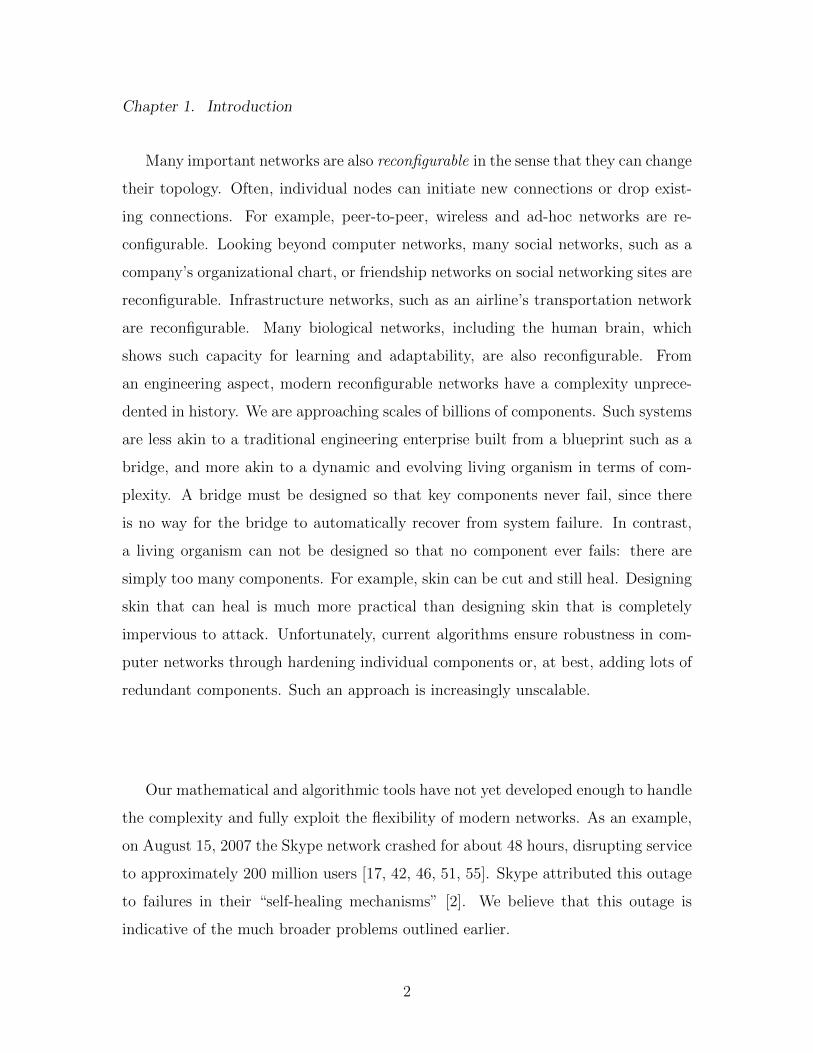
Many important networks are also reconfigurable in the sense that they can change
their topology. Often, individual nodes can initiate new connections or drop exist-
ing connections. For example, peer-to-peer, wireless and ad-hoc networks are re-
configurable. Looking beyond computer networks, many social networks, such as a
company’s organizational chart, or friendship networks on social networking sites are
reconfigurable. Infrastructure networks, such as an airline’s transportation network
are reconfigurable. Many biological networks, including the human brain, which
shows such capacity for learning and adaptability, are also reconfigurable. From
an engineering aspect, modern reconfigurable networks have a complexity unprece-
dented in history. We are approaching scales of billions of components. Such systems
are less akin to a traditional engineering enterprise built from a blueprint such as a
bridge, and more akin to a dynamic and evolving living organism in terms of com-
plexity. A bridge must be designed so that key components never fail, since there
is no way for the bridge to automatically recover from system failure. In contrast,
a living organism can not be designed so that no component ever fails: there are
simply too many components. For example, skin can be cut and still heal. Designing
skin that can heal is much more practical than designing skin that is completely
impervious to attack. Unfortunately, current algorithms ensure robustness in com-
puter networks through hardening individual components or, at best, adding lots of
redundant components. Such an approach is increasingly unscalable.
Our mathematical and algorithmic tools have not yet developed enough to handle
the complexity and fully exploit the flexibility of modern networks. As an example,
on August 15, 2007 the Skype network crashed for about 48 hours, disrupting service
to approximately 200 million users [17, 42, 46, 51, 55]. Skype attributed this outage
to failures in their “self-healing mechanisms” [2]. We believe that this outage is
indicative of the much broader problems outlined earlier.
2

Chapter 1. Introduction
In the following chapters, we will propose some algorithms for self-healing. Infor-
mally, we define self-healing to be maintenance of certain properties within desirable
bounds by the nodes in a network suffering from failures or under attack. As the
name implies, self-healing has to be initiated and executed by the nodes themselves.
As such, the algorithms we have proposed here are fully distributed. Equivalenty we
can say that a self-healing system, when starting from a correct state, can only be
temporarily out of a correct state i.e. it recovers to a correct state, in presence of
attacks. Self-healing is one of the so called ‘Self-*’ properties which systems such as
autonomic systems may be required to have. Section 1.5.1 has a brief discussion on
these properties.
One approach towards self-healing is to add additional capacity or rerouting in
anticipation of failures. There has been plenty of work which has followed this
approach. However, there are obvious limitations including wastage of resources and
limitations on additional capacity. In this Dissertation, we have adopted a responsive
approach. Our approach is responsive in the sense that it responds to an attack
(or component failure) by changing the topology of the network. This approach
works irrespective of the initial state of the network, and is thus orthogonal and
complementary to traditional non-responsive techniques.
Informally, the model we adopt in this work is as follows. We assume that the
network is initially a connected graph over n nodes. An adversary repeatedly attacks
the network. This adversary knows the network topology and our algorithm, and it
has the ability to delete arbitrary nodes from the network or insert a new node in
the system which it can connect to any subset of the nodes currently in the system.
However, we assume the adversary is constrained in that in any time step it can only
delete or insert a single node. Following that, the self-healing algorithm has a short
time to reconfigure and heal the network by adding edges between remaining nodes
before the next act of the adversary. Our model captures what can happen when a
3

Chapter 1. Introduction
worm or software error propagates through the population of nodes. This model is
described in more detail Section 1.2.
1.1 Naive self-healing
Even in a very simple setting, we need to be smart about reconfiguring. Suppose
we are trying to maintain a property such as connectivity of the network but our
algorithm is not very sophisticated. Then, it may be very easy for the adversary to
force the algorithm to cause high degree increase (which may lead to overload and
eventual network breakdown) or increase in distances between nodes (which may
lead to poor communication). Figure 1.1 shows a naive algorithm attempting to heal
the network by using only a small number of edges at each timestep. However, node
v in the figure ends up increasing its degree by 3 over a course of 3 deletions. Thus,
a naive algorithm could yield a degree increase as high as θ(n).
1.2 Model of self-healing
Our general model of self-healing is shown in Figure 1.2. The specific models used
in our algorithms are special cases of this model, differing mainly in the way the
success metrics of the graph properties are presented. This model is very similar
to the model described in Figure 3.2.1. Let G = G0 be an arbitrary graph on
n nodes, which represent processors in a distributed network. In each step, the
adversary either deletes or adds a node. After each deletion, the algorithm gets to
add some new edges to the graph, as well as deleting old ones. At each insertion,
the processors follow a protocol to update their information. The algorithm’s goal
is to maintain the chosen graph properties within the desired bounds. At the same
time, the algorithm wants to minimize the resources spent on this task. Initially,
4

Chapter 1. Introduction
v
(a) First deletion
v
(b) Neighbors detect dele-tion
v
(c) Reconnection: v in-creases degree
v
(d) Second deletion
v
(e) Detection
v
(f) v’s degree increases by 2
v
(g) Third deletion
v
(h) Detection
v
(i) v’s degree increases by 3
Figure 1.1: A sequence of 3 deletions and healings using a naive algorithm. A nodemarked red is deleted by the adversary. The neighbors of the deleted node reconnect(golden edges) to maintain connectivity. Notice node v increases its degree by 3.
each processor only knows its neighbors in G0, and is unaware of the structure of
the rest of G0. After each deletion or insertion, only the neighbors of the deleted or
inserted vertex are informed that the deletion or insertion has occured. After this,
processors are allowed to communicate by sending a limited number of messages to
5

Chapter 1. Introduction
their direct neighbors. We assume that these messages are always sent and received
successfully. The processors may also request new edges be added to the graph. The
only synchronicity assumption we make is that no other vertex is deleted or inserted
until the end of this round of computation and communication has concluded. To
make this assumption more reasonable, the per-node communication cost should be
very small in n (e.g. at most logarithmic).
We also allow a certain amount of pre-processing to be done before the first attack
occurs. This may, for instance, be used by the processors to gather some topological
information about G0, or perhaps to coordinate a strategy. Another success metric
is the amount of computation and communication needed during this preprocessing
round. For our success metrics, we compare the graphs at time T : the actual graph
GT to the graph G′T which is the graph with only the original nodes (those at G0)
and insertions without regard to deletions and healing. This is the graph which
would have been present if the adversary was not doing any deletions and (thus) no
self-healing algorithm was active. This is the natural graph for comparing results.
Figure 1.3 shows an example of G′T and a corresponding GT . The figure also shows,
in G′T , the nodes and edges inserted and deleted, and in GT , the edges inserted by
the healing algorithm, as the network evolved over time.
6

Chapter 1. Introduction
Figure 1.2: The general distributed Node Insert, Delete and Network Repair Model.
Each node of G0 is a processor.Each processor starts with a list of its neighbors in G0.Pre-processing: Processors may exchange messages with their neighbors.for t := 1 to T do
Adversary deletes a node vt from Gt−1 or inserts a node vt into Gt−1, formingHt.if node vt is inserted then
The new neighbors of vt may update their information and exchange mes-sages with their neighbors.
end ifif node vt is deleted then
All neighbors of vt are informed of the deletion.Recovery phase:Nodes of Ht may communicate (asynchronously, in parallel) with their im-mediate neighbors. These messages are never lost or corrupted, and maycontain the names of other vertices.During this phase, each node may add edges joining it to any other nodesas desired. Nodes may also drop edges from previous rounds if no longerrequired.
end ifAt the end of this phase, we call the graph Gt.
end for
Success metrics: Minimize the following “complexity” measures:Consider the graph G′ which is the graph consisting solely of the original nodesand insertions without regard to deletions and healings. Graph G′t is G′ attimestep t (i.e. after the tth insertion or deletion).
1. Graph properties/invariants.The graph properties/ invariants we are trying to preserve. e.g. Degreeincrease: maxv∈G degree(v,GT )/degree(v,G′T )
2. Communication per node. The maximum number of bits sent by asingle node in a single recovery round.
3. Recovery time. The maximum total time for a recovery round, assumingit takes a message no more than 1 time unit to traverse any edge and wehave unlimited local computational power at each node.
7

Chapter 1. Introduction
(a) G′T : Nodes in red (dark gray ingrayscale) deleted, and nodes in green(patterned) inserted, by the adver-sary.
(b) GT : The actual graph. Edgesadded by the healing algorithmshown in gold (light shaded ingrayscale) color.
Figure 1.3: Graphs at time T. G′T : The graph of initial nodes and insertions overtime, GT : The actual healed graph.
1.3 Healing by Reconstruction Trees
h
RTda
j
x
f ge h
cb
e f g
Figure 1.4: Deleted node x (in red, crossed) replaced by a Reconstruction Tree, whichis a structure formed by its neighbors (a, b, c, d, j).
Our algorithms (DASH,ForgivingTree,ForgivingGraph) use the same basic prin-
ciple: when a node is deleted, replace it by a tree based structure formed from its
8

Chapter 1. Introduction
neighbors, as shown in Figure 1.4. This structure we call the Reconstruction Tree
(RT), and thus, we can also call these algorithms Reconstruction Tree healing algo-
rithms. It turns out that trees are a natural choice for the graph properties we have
tried to maintain. A balanced tree is a structure which has low distance between
nodes (at most 2 log2 n for a balanced binary tree) while each node has a small degree
(at most 3 for a binary tree). At the same time, coming up with the suitable RTs
and maintaining them over the run of the algorithm is quite a significant challenge.
1.4 Our Results
In our algorithms, we have focused on some fundamentally important properties:
maintaining connectivity, ensuring low degree increase for all nodes, and simultane-
ously, in later algorithms, ensuring low increase of diameter (or a stronger property,
the stretch) of the network. Figure 1.4 (repeated as Figure 2.9) shows a series of
snapshots from a simulation of our algorithm called DASH (Chapter 2). Notice that
the network stays connected, and no individual node gets a large number of extra
edges during healing.
We have developed three different distributed self-healing algorithms, whose re-
sults are optimal (i.e. with a matching lower bound) for their particular objectives.
All of them fulfill the objectives of maintaining connectivity in the network in face of
adverserial attacks, and low degree increase for individual nodes. These algorithms
were presented at reputed conferences and have been well received by the academic
community. These algorithms are:
• DASH: Degree Assisted Self Healing : DASH guarantees network connectivity
and degree increase of at most 2 log n, where n is the number of nodes initially
in the network. DASH is locality-aware i.e. only the immediate neighbors of a
9

Chapter 1. Introduction
(a) single deletion (b) 10 deletions (c) 30 deletions
(d) 40 deletions (e) 50 deletions (f) 60 deletions
(g) 70 deletions (h) 80 deletions (i) 90 dele-tions
Figure 1.5: A timeline of deletions and self healing in a network with 100 nodes. Thegray edges are the original edges and the red edges are the new edges added by ourself-healing algorithm.
10

Chapter 1. Introduction
deleted node are involved in reconstruction. Also, the healing algorithm always
adds in less edges than the adversary has removed from the system. Empirical
results show that DASH performs well in practice on power-law networks. This
is joint work with Jared Saia. An earlier version [53] was presented at the
conference IEEE International Parallel & Distributed Processing Symposium
2008.
• ForgivingTree: This algorithm efficiently maintains a special spanning tree
which guarantees at worst a constant additive degree increase and diameter
increase of only a log ∆ factor, where ∆ is the maximum degree of a node in
the original network, by a system of inheritance and wills. This is work jointly
done with Tom Hayes, Navin Rustagi and Jared Saia. An earlier version [24]
was presented at the conference ACM Principles of Distributed Computing
2008.
• ForgivingGraph: This algorithm efficiently maintains a general graph of the
network, handling both deletions and insertions, while guaranteeing at worst
a constant multiplicative degree increase and the simultaneously challenging
property of a low (log n) factor stretch (maximum distance increase between
any two nodes). Also, we introduce a novel mergable data structure called
half-full trees(haft) having a one-to-one correspondence with binary numbers,
with the merge corresponding to binary addition. This is joint work with Tom
Hayes and Jared Saia. An earlier version [23] was presented at the conference
ACM Principles of Distributed Computing 2009.
Table 1.1 gives a comparison of these self-healing algorithms with regards to
various criteria including methods of adverserial attack, properties maintained, and
costs of the algorithm. Many important open questions remain and there are many
promising directions towards which our work can be extended. Some of these are
discussed in the last chapter (Chapter 5).
11

Chapter 1. Introduction
Adversarial Attack Property boundedDeletion Insertion Connec-
tivityDegree(orig: d)∗
Diameter(orig: D)∗
Stretch
DASH X X X d+ 2 log n — —Forgiving Tree X × X d+ 3 D log ∆ —Forgiving Graph X X X 3d D log n log n∗ ‘orig:’ the original value of the property in the graph (i.e. the value in the graph
G′ in our model)
CostsRepair time # Msgs per dele-
tionMsg size match
lowerbound‡
locality(hops)]
DASH O(log n) † O(δ log n+ log2 n) † O(log n) X 1Forgiving Tree O(1) O(δ) O(log n) X 2
Forgiving Graph O(log δ log n) O(δ log n) O(log2 n) X log n† with high probability, and amortized over O(n) deletions.‡ The lower bounds differ according to the properties being bounded.] Number of hops from the deleted node to nodes involved in repair.
Table 1.1: Comparison of our self-healing Algorithms. d is the degree of an individualnode, ∆ is the maximum degree of a node in the graph, and δ is the degree of thedeleted node.
1.5 Related Work
There have been numerous papers that discuss strategies for adding additional ca-
pacity or rerouting in anticipation of failures [3, 15, 18, 29, 49, 58, 61]. Results
that are responsive in some sense include the following. Medard, Finn, Barry, and
Gallager [44] propose constructing redundant trees to make backup routes possible
when an edge or node is deleted. Anderson, Balakrishnan, Kaashoek, and Morris [1]
modify some existing nodes to be RON (Resilient Overlay Network) nodes to detect
failures and reroute accordingly. Some networks have enough redundancy built in
so that separate parts of the network can function on their own in case of an at-
12

Chapter 1. Introduction
tack [20]. In all these past results, the network topology is fixed. In contrast, our
algorithms add or deletes edges as node failures occur. Moreover, our algorithms do
not dictate routing paths or specifically require redundant components to be placed
in the network initially.
There has also been recent research in the physics community on preventing
cascading failures. In the model used for these results, each vertex in the network
starts with a fixed capacity. When a vertex is deleted, some of its “load” (typically
defined as the number of shortest paths that go through the vertex) is diverted to the
remaining vertices. The remaining vertices, in turn, can fail if the extra load exceeds
their capacities. Motter, Lai, Holme, and Kim have shown empirically that even a
single node deletion can cause a constant fraction of the nodes to fail in a power-
law network due to cascading failures[25, 48]. Motter and Lai propose a strategy
for addressing this problem by intentional removal of certain nodes in the network
after a failure begins [47]. Hayashi and Miyazaki propose another strategy, called
emergent rewirings, that adds edges to the network after a failure begins to prevent
the failure from cascading[22]. Both of these approaches are shown to work well
empirically on many networks. However, unfortunately, they perform very poorly
under adversarial attack.
A responsive approach was followed by the authors in [9, 10], which proposed a
simple line algorithm for self-healing to maintain network connectivity. This algo-
rithm has obvious drawbacks with regard to properties such as diameter maintenance
but has served as a useful starting point for our research.
1.5.1 Self-healing and Self-* properties
The importance of self-healing in systems is worth mentioning. As an example, self-
healing is one of the main components of IBM’s autonomic systems initiative [27, 28].
13

Chapter 1. Introduction
Autonomic computing itself is one of the building blocks of pervasive computing, an
anticipated future computing model in which tiny - even invisible - computers will
be all around us, communicating through increasingly interconnected networks [60].
Self-healing forms one of the eight crucial elements in IBM’s autonomic computing
vision. Self-healing is one of the self-* properties that a system can possess, where
the ‘*’ in self-* is a wildcard character that can take on many different forms. IBM’s
vision often refers to an autonomic computing system as a self-managing system that
has the so-called self-CHOP properties: self-configuring, self-healing, self-optimizing,
and self-protecting. Often, self-management is a generic term which implies the sys-
tem has at least one of the other self-* properties i.e. it has some desired autonomic
behavior [8].
In the distributed systems world, perhaps the most well-known self-* property
is self-stabilization [12, 13, 14, 57]. Self-stabilization was introduced by Djikstra in
1974 [12]. A self-stabilizing system is a system which, starting from an arbitrary
state and being affected by adversarial transient failures, can, in finite time, recover
to a correct state. Often, self-stabilization does not take code corruption (byzantine
behavior) or fail-stop failures (node crashes) into account. A self-healing system,
when starting from a correct state, can only be temporarily out of a correct state
i.e. it recovers to a correct state, in presence of some adversarial attacks including
node removal. Other self-* properties, often broadly defined, include self-scaling,
self-repairing (similar to self-healing), self-adjusting (similar to self-managing), self-
aware/self-monitoring, self-immune, self-containing [8].
1.6 Structure of the document
The next three chapters are self-contained presentations of the three algorithms with
an occasional reference to the Introduction. Chapter 2 presents DASH, chapter 3
14

Chapter 1. Introduction
describes ForgivingTree, chapter 4 presents ForgivingGraph. Chapter 5 sketches
some open problems and possible directions. For chapter 2 of this dissertation, we
gratefully acknowledge the help of Iching Boman, Dr. Deepak Kapur and his class
Introduction to Proofs, Logic and Term-rewriting, and the UNM Computer Science
Theory Seminar.
15

Chapter 2
DASH
But he said what mattered most of
all was the dash between those years
The Dash Poem
Linda Ellis
This chapter presents the first of our self-healing algorithms called DASH (short
for Degree Assisted Self-Healing, which first appeared at IEEE International Parallel
& Distributed Processing Symposium 2008 [53] To recap, we consider the problem of
self-healing in networks that are reconfigurable in the sense that they can change their
topology during an attack. Our goal is to maintain connectivity in these networks,
even in the presence of repeated adversarial node deletion, by carefully adding edges
after each attack. We present a new algorithm, DASH which provably ensures that:
1) the network stays connected even if an adversary deletes up to all nodes in the
network; and 2) no node ever increases its degree by more than 2 log n, where n is the
number of nodes initially in the network. DASH is fully distributed; adds new edges
only among neighbors of deleted nodes; and has average latency and bandwidth
costs that are at most logarithmic in n. DASH has these properties irrespective
of the topology of the initial network, and is thus orthogonal and complementary
16

Chapter 2. DASH
to traditional topology-based approaches to defending against attack. The detailed
model used in DASH and its relation to the general model we described in Section 1.2
is given in Section 2.1.
We also prove lower-bounds showing that DASH is asymptotically optimal in
terms of minimizing maximum degree increase over multiple attacks. Finally, we
present empirical results on power-law graphs that show that DASH performs well in
practice, and that it significantly outperforms naive algorithms in reducing maximum
degree increase.
2.1 Introduction
Earlier in Chapter 1, we have made a case for better “self-healing mechanisms” and
of the need for using responsive approaches for maintaining robust networks. There
are many desirable invariants to maintain in the face of an attack. Here we focus only
on the simplest and most fundamental invariants: maintaining network connectivity
and ensuring low node degree increase.
Our Model: We now describe our model of attack and network response. We
assume that the network is initially a connected graph over n nodes. We assume
that every node knows not only its neighbors in the network but also the neighbors
of its neighbors i.e. neighbor-of-neighbor (NoN) information. In particular, for all
nodes x,y and z such that x is a neighbor of y and y is a neighbor of z, x knows
z. There are many ways that such information can be efficiently maintained, see
e.g. [43, 50].
We assume that there is an adversary that is attacking the network. This ad-
versary knows the network topology and our algorithm, and it has the ability to
delete carefully selected nodes from the network. However, we assume the adversary
17

Chapter 2. DASH
is constrained in that in any time step it can only delete a small number of nodes
from the network1. We further assume that after the adversary deletes some node
x from the network, that the neighbors of x become aware of this deletion and that
they have a small amount of time to react.
When a node x is deleted, we allow the neighbors of x to react to this deletion
by adding some set of edges amongst themselves. We assume that these edges can
only be between nodes which were previously neighbors of x. This is to ensure
that, as much as possible, edges are added which respect locality information in the
underlying network. We assume that there is very limited time to react to deletion
of x before the adversary deletes another node. Thus, the algorithm for deciding
which edges to add between the neighbors of x must be fast and localized.
This model can be seen as a special case of our general model (Section 1.2). We
do not explicitly discuss node insertions in our further treatment but assume we
begin with a connected graph of n vertices. DASH can easily handle insertions in
a natural way, and thus, as long as the number of insertions are O(n), our bounds
hold. Also, for the same reason, for our bounds, we need only compare our graph
properties in the present graph at timestep t (Gt), to the initial graph G0 which has
n vertices (notice n is the maximum number of nodes the network will have in this
model).
Our Results: We introduce an algorithm for self-healing of reconfigurable networks,
called DASH (an acronym for Degree Assisted Self-Healing). DASH is locality-aware
in that it uses only the neighbors of the deleted node for reconnection. We prove
that DASH maintains connectivity in the network, and that it increases the degree
of any node by no more than O(logn). During reconnection of nodes, our algorithm
1Throughout this chapter, for ease of exposition, we will assume that the adversarydeletes only one node from the network before the algorithm responds. However, our mainalgorithm, DASH, can easily handle the situation where any number of nodes are removed,so long as the neighbor-of-neighbor graph remains connected.
18

Chapter 2. DASH
uses only local information, therefore, it is scalable and can be implemented in a
completely distributed manner. Algorithm DASH is described as Algorithm 2.2.1
in Section 2.2. The main characteristics of DASH are summarized in the following
theorem that is proved in Section 2.2.
Theorem 2.1. DASH guarantees the following properties even if up to all the nodes
in the network are deleted:
• The degree of any vertex is increased by at most 2 log n.
• The number of messages any node of initial degree d sends out and receives is
no more than 2(d+ 2 log n) lnn with high probability2 over all node deletions.
• The latency to reconnect is O(1) after attack; and the amortized latency to
update the state of the network over θ(n) deletions is O(log n) with high prob-
ability.
We also prove (in Section 2.3) the following lower bound that shows that DASH is
asymptotically optimal.
Theorem 2.2. Consider any locality-aware algorithm that increases the degree of
any node after an attack by at most a fixed constant. Then there exists a graph and a
strategy of deletions on that graph that will force the algorithm to increase the degree
of some node by at least log n.
We also present empirical results (in Section 2.4) showing that DASH performs
well in practice and that it significantly outperforms naive algorithms in terms of
reducing the maximum degree increase. Finally (in Section 2.4) we describe SDASH,
a heuristic based on DASH that we show empirically both keeps node degrees small
and also keeps shortest paths between nodes short.
2Throughout this text, we use the phrase with high probability (w.h.p) to mean withprobability at least 1− 1/nC for any fixed constant C.
19

Chapter 2. DASH
In this chapter, we build on earlier work done in [9, 10], which proposed a simple
line algorithm for self-healing to maintain network connectivity.
Table of Contents: The rest of this chapter is organized as follows. Section 2.2
describes the algorithm DASH, and its theoretical properties. Section 2.3 gives a
lower bound on locality-aware algorithms. Section 2.4 gives empirical results for
DASH, and several other simple algorithms on random power-law networks. It also
describes and gives results for SDASH. We conclude and give areas for future work
in Section 2.5.
2.2 DASH: An Algorithm for Self-Healing
In this Section, we describe DASH and prove certain properties about it. In brief,
when a deletion occurs, DASH asks the neighbors of the deleted node to reconnect
themselves into a certain kind of complete binary tree. Then messages are propagated
so that the nodes can keep track of which connected component they belong to.
Let the actual network at a particular time step be G(V,E). Let Eh be the edges
(i.e. healing edges), that have been added by the algorithm up to that time step
(note Eh ⊆ E). Let Gh = (V,Eh). We show that Gh is a forest in Lemma 2.1.
2.2.1 DASH: Degree Assisted Self-Healing
As the acronym suggests, DASH employs information of previous degree increase
to control further degree increase for a node. When a deletion occurs, we assume
the neighbors of the deleted node are able to detect the deletion. Then they em-
ploy DASH to heal. To maintain connectivity, DASH connects the neighbors of a
deleted node as a binary tree. The tree is structured so that the vertices which
20

Chapter 2. DASH
have incurred the maximum degree increase previously get to be leaves and thus not
increase their degree in this round. Notice that at least half the vertices in a binary
tree are leaves. The nodes maintain information about the virtual network and their
connected component in this network. The algorithm tries to use only a single node
from each component during reconnection and thus adds only a low number of new
edges during healing.
To describe DASH we give some definitions. Let N(v,G) be the neighbors of
vertex v in the graph G representing the real network. Let N(v,Gh) be the neighbors
of vertex v in graph Gh consisting of the edges added by the healing algorithm. Let
δ(v) be the degree increase of the vertex v compared to its initial degree. Note that
this is not the same as the degree of v in Gh.
When a node v is deleted, partition on the basis of their ID all the neighbors
of v in G (not having the same ID as v). Let UN(v,G) (Unique Neighbors) be the
set having one representative from each of the partitions. If there is more than one
node as a possible representative from a partition, we include the one with the lowest
initial ID.
Note that UN(v,G) ∩N(v,Gh) = φ and UN(v,G) ∪N(v,Gh) ⊆ N(v,G) . The
ID of a node allows us to keep track of which connected component in Gh it belongs
to. The lowest ID of any node in that component is broadcast and all the nodes in
the component take on this ID.
Our main results about DASH are stated in Theorem 2.1.
Theorem 2.1. DASH is a distributed algorithm with the following properties:
• The degree of any vertex is increased by at most 2 log n.
• The latency to reconnect is O(1).
21

Chapter 2. DASH
1: Init: for given network G(V,E), Initialize each vertex with a random number
ID between [0,1] selected uniformly at random.
2: while true do
3: If a vertex v is deleted, do
4: Nodes in UN(v,G)∪N(v,Gh) are reconnected into a complete binary tree. To
connect the tree, go left to right, top down, mapping nodes to the complete
binary tree in increasing order of δ value.
5: Let MINID be the minimum ID of any node in UN(v,G)∪N(v,Gh). Prop-
agate MINID to all the nodes in the tree of UN(v,G)∪N(v,Gh) in Gh. All
these nodes now set their ID to MINID.
6: end while
Algorithm 2.2.1: DASH: Degree-Based Self-Healing
• The number of messages any node of degree d sends out and receives is no more
than (2d+ 2 log n) lnn with high probability over all node deletions.
• The amortized latency for ID propagation is O(logn) with high probability
over all node deletions.
2.2.2 Towards the proof of Theorem 2.1
For analysis, we use the following definitions:
• Let T (x, y) be the tree in Gh − y that contains x.
• Each vertex v will have a weight, w(v). The weight of a vertex will start at
1 and may increase during the algorithm. If v is deleted, w(v) is added to an
arbitrarily chosen neighbor in Gh.
• Let W (S) =∑v∈V
w(v), for a graph S(V,E) i.e. the sum of the weights of all
vertices in S.
22

Chapter 2. DASH
• For vertex v, let rem(v) =
∑u∈N(v,Gh)
W (T (u, v)) − maxu∈N(v,Gh)
(W (T (u, v))) + w(v).
We will show that as the degree of a vertex increases in our algorithm, so will
the rem value of that vertex. Intuitively rem(v) is large when removing v from
its tree in Gh gives rise to many connected components with large weight.
Lemma 2.1. The edges added by the algorithm, Eh, form a forest.
Proof. We prove this by induction on the number of nodes deleted.
Base Case: Initially, Gh is a forest because Eh is empty.
We note that Eh and Gh change only when a deletion occurs. Consider the ith
deletion and let v be the node deleted.
Let v belong to tree Tv in Gh just prior to the deletion of v. Now, for all x, y ∈
N(v,Gh) x and y are not connected in Eh since that would have implied the existence
of a cycle through v contradicting the Inductive Hypothesis. Note also that for all
z ∈ UN(v,G), z /∈ Tv. Since we select only 1 node from each tree Ti in which v
had a neighbor, no pair of nodes in UN(v,G) ∪ N(v,Gh) are connected in Gh. We
reconnect all the nodes in UN(v,G) ∪N(v,Gh) in a Binary Tree and propagate the
minimum ID. Since we are adding edges between nodes which previously were in
separate connected components in Gh, no cycles are introduced. Hence, Gh remains
a forest.
23

Chapter 2. DASH
Lemma 2.2. For any vertex v, rem(v) is non-decreasing over any vertex deletion
where v has not been deleted.
Proof. By Lemma 2.1, every vertex v in Gh belongs to some tree, which we will call
Tv. For every Tv in Gh, W (Tv) is the sum of the weights of all vertices in Tv.
By definition, rem(v) =
∑u∈N(v,Gh)
W (T (u, v)) − maxu∈N(v,Gh)
(W (T (u, v))) + w(v).
Therefore,
rem(v) = W (Tv)− maxu∈N(v,Gh)
W (T (u, v))
Observe first that W (Tv) cannot decrease even when there is a deletion in Tv
because the deleted vertex’s weight is not “lost”, but added to some member of Tv.
Since W (Tv) cannot decrease, rem(v) can only decrease if the maximum subtree
weight increases more than W (Tv). Since the maximum subtree is a subset of the
tree, Tv, any increases or decreases in the maximum subtree is also counted in W (Tv).
Thus, rem(v) cannot decrease.
24

Chapter 2. DASH
Lemma 2.3. For any node v, for all nodes q ∈ N(v,Gh) , W (T (v, q)) ≥ rem(v).
m
r
l
v
Figure 2.1: W (T (v,m)) ≥ rem(v).
Proof. For all nodes q,
W (T (v, q)) =∑
u∈N(v,Gh)u6=q
W (T (u, v)) + w(v)
≥∑
u∈N(v,Gh)
W (T (u, v))
− maxu∈N(v,Gh)
W (T (u, v)) + w(v)
= rem(v)
For example, in figure 2.1, W (T (V,M)) = W (T (L, V )) + W (T (R, V )) + w(v) ≥
rem(v).
25

Chapter 2. DASH
Lemma 2.4. For any node v, rem(v) ≥ 2δ(v)/2, where δ(v), as defined earlier, is the
degree increase of the vertex v in G.
Proof. Let t be the number of rounds of healing where a round is a single adversarial
deletion followed by self-healing by DASH. We prove this lemma by induction on t.
Let Ght, remt(v) and δt(v) be Gh, rem(v) and δ(v) respectively at time t.
Base Case: t = 0: In this case, all nodes v have δ(v) = 0; rem(v) = 1. Thus,
rem(v) ≥ 20.
Inductive Step: Consider the network at round t. We assume by the inductive
hypothesis that for all nodes v in Gh, remt−1(v) ≥ 2δt−1(v)/2. Our goal is to show
that remt(v) ≥ 2δt(v)/2.
Suppose node x was deleted at round t. According to our algorithm, some or all
of the neighbors of x will be reconnected as a binary tree. Let us call this tree RT
(short for Reconstruction Tree). Let T (x, y) be the tree in Gh(t−1) − y that contains
x, and T ′(x, y) be the tree in Ght − y that contains x.
Consider a surviving vertex v. If v is not a part of RT, then by a simple application
of lemma 2.2, our induction holds. If v is a part of RT, there are 3 possibilities:
1. v is a leaf node in RT
The degree of v did not change. Thus, δt(v) = δt−1(v). By Lemma 2.2,
remt(v) ≥ remt−1(v). Thus, using the induction hypothesis, remt(v) ≥ 2δt(v)/2.
2. v is the root of RT
If v has only one child in RT, then this is the same as the previous case with the
parent and child role reversed and the induction holds. Let us consider the case
26

Chapter 2. DASH
w1
w2v
z
x
H
v
z
w1 w2
H’
Figure 2.2: node v is the root, with 2 children
when v has two children in RT. Now, δt(v) has increased by 1. Let z be the
neighbor of v such thatW (T (z, v)) is the largest among all neighbors of v except
x. Note that W (T ′(z, v)) = W (T (z, v)), since this subtree was not involved
in the reconstruction. Consider the possibly empty subtree of v rooted at z.
Let the two children of v in RT be w1 and w2, as illustrated in figure 2.2. By
our algorithm, we know that δt−1(w1) ≥ δt−1(v) and δt−1(w2) ≥ δt−1(v). Thus,
using the inductive hypothesis and lemma 2.3, we have that W(T(w1, x)) ≥
remt−1(w1) ≥ 2δt−1(w1)/2 and W(T(w2, x)) ≥ remt−1(w2) ≥ 2δt−1(w2)/2. By
lemma 2.2, this implies that in Ght,
W (T′(w1, v)) ≥ 2δt−1(w1)/2 ≥ 2δt−1(v)/2
W (T′(w2, v)) ≥ 2δt−1(w2)/2 ≥ 2δt−1(v)/2
Assume without loss of generality that W(T′(w1, v)) ≤ W(T′(w2, v)). There
are two cases:
(a) W(T(z, v)) < W(T′(w1, v))
In this case remt−1(v) did not include W(T(x, v)). But remt(v) will
include W(T′(w1, v)) Hence,
27

Chapter 2. DASH
remt(v) ≥ remt−1(v) + W(T′(w1, v))
≥ 2δt−1(v)/2 + 2δt−1(v)/2
= 2(δt−1(v)+2)/2
= 2(δt(v)+1)/2
(b) W(T(z, v)) ≥W(T′(w1, v))
In this case remt(v) will include W(T′(w1, v)) and the smaller of
W(T′(w2, v)) and W(T′(z, v)). Note that by Lemmas 2.3 and 2.2, the in-
ductive hypothesis, and the fact that δt−1(w1) ≥ δt−1(v), W(T ′(w1, v)) ≥
remt(w1) ≥ remt(w1) ≥ 2δt−1(w1)/2 ≥ 2δt−1(v)/2.
Also, since by assumption W(T ′(w2, v)) ≥ W(T ′(w1, v)), we know that
W(T ′(w2, v)) ≥ 2δt−1(v)/2.
Further, since W(T ′(z, v)) = W(T (z, v)) ≥ W(T ′(w1, v)) we know that
W(T ′(z, v)) ≥ 2δt−1(v)/2.
Hence,
remt(v) ≥ 2δt−1(v)/2 + 2δt−1(v)/2
= 2(δt−1(v)+2)/2
= 2(δt(v)+1)/2
3. v is an internal node in T ′
For node v to become an internal node, the deleted neighbor x must have at
least three other neighbors. Three neighbors of x are shown as C1, C2 and P
in the figures 2.3 and 2.4. Also, now v’s degree can increase by 1, as illustrated
in figure 2.3, or by 2, as illustrated in figure 2.4. Let us consider these cases
separately:
(a) δt(v) = δt−1(v) + 1
28

Chapter 2. DASH
vx
H H’
c1
c2
p
c1
p
c2
p2v
Figure 2.3: Internal node v with 1 child
vx
c1
c2
p
c1
v
p
c2
H H’
Figure 2.4: Internal node v with 2 children
This can only happen when v has a parent and a single child in RT as in
figure 2.3. Let P be the parent of v and C1 the child of v. C1 has to be
a leaf node since the tree is complete and v has only one child. Observe
that there exists at least one leaf node besides C1 in the tree, accessible
to v only via P . Let this node be C2 and let P2 be its parent. Note that
P2 and P may even be the same node. In our algorithm, any leaf node
in RT has a δ value no less than the δ value of any internal node. Thus,
δt−1(C1) ≥ δt−1(v); and
δt−1(C2) ≥ δt−1(v)
29

Chapter 2. DASH
These inequalities, Lemmas 2.2 and 2.3, and the Inductive Hypothesis,
imply that
W(T′(C1, v)) ≥ remt(C1)
≥ remt−1(C1)
≥ 2δt−1(v)/2;
W(T′(C2, P2)) ≥ remt(C2)
≥ remt−1(C2)
≥ 2δt−1(v)/2;
W(T(v, x)) ≥ remt(v)
≥ remt−1(v)
≥ 2δt−1(v)/2.
Since remt(v) can exclude at most one of W (T ′(C1, v)), W (T ′(C2, P2))
and W (T (v, x)),
remt(v) ≥ 2δt−1(v)/2 + 2δt−1(v)/2
= 2(δt(v)+1)/2
(b) δt(v) = δt−1(v) + 2
In this case v has two children in RT, C1 and C2, as illustrated in figure
2.4. The analysis is similar to the case above. The value remt(v) can
exclude at most one of W (T ′(C1, v)), W (T ′(C2, v)) and W (T (v, x)) and
we can show that all three of these values are at least 2δt−1(v)/2. Thus,
remt(v) ≥ 2(δt(v))/2.
Hence, the induction holds.
30

Chapter 2. DASH
Lemma 2.5. For all vertices v, rem(v) is always no more than n.
Proof. No vertex is counted twice in a rem value since the subtrees of a vertex
are disjoint. Since the number of vertices in the subtrees cannot be more than the
number of vertices remaining, the rem value is always no more than the sum of the
weights of all undeleted vertices in Gh.
Define W ∗ to be the sum of weights of all undeleted vertices in Gh. After initial-
ization, W ∗ = n, since there are n vertices. At each step of the algorithm, W ∗ = n
, since the weight of the deleted vertex is added to one of the remaining vertices.
Thus, for node v, rem(v) ≤ n.
Lemma 2.6. DASH increases the degree of any vertex by at most O(log n).
Proof. Every vertex v starts with rem(v) = w(v) = 1. We know that rem(v) ≥ 2δ(v)/2
by Lemma 2.4. since rem(v) is at most n, 2δ(v)/2 ≤ n . Taking log of both sides,
δ(v)/2 ≤ log n. Solving for δ(v) gives δ(v) ≤ 2 log n.
Lemma 2.7. The latency to reconnect the network in DASH is O(1).
Proof. During the reconnection process, DASH requires communication only between
nodes one hop away, thus, the latency is just O(1).
31

Chapter 2. DASH
Lemma 2.8. The number of messages any node of initial degree d sends out and
receives is no more than 2(d + 2 log n) lnn with high probability over all node dele-
tions.
Proof. In DASH, after the reconnections have been made, messages are sent out by
nodes when the minimum ID has to be propagated. With similarity to the record
breaking problem [19](Section 2.2.3), it is easily shown that w.h.p., a node has its
ID reduced no more than 2 lnn times, where the record is the node’s ID. These
are the only messages the node needs to transmit or receive. Each time its ID
changes, the node sends this message to all its neighbors, Thus, it sends or receives
O((d+ log n) lnn) messages, since the final degree of the node is at most d+ 2 log n.
Lemma 2.9. The amortized latency for ID propagation is O(log n) with high prob-
ability over all node deletions.
Proof. Again, with similarity to the record breaking problem, a node sends messages
to its neighbors (neighbors, by definition, are a single hop away) only O(log n) times
with high probability. Thus, messages are transmitted O(n log n) times over all the
nodes. Over O(n) deletions, this implies that the amortized latency for messages
(involving ID propagation) is only O(log n) .
2.2.3 The Record Breaking Problem
Here we recap the well known record breaking problem. Given a sequence of deleted
vertices, v1, v2, ..., vn, we define id(vj) (j ≤ n) to be a record value if id(vj) < id(vi)
for all 1 ≥ i < j.
32

Chapter 2. DASH
Let X1, X2, ..., Xn be indicator random variable:
Xj =1 if id(vj) is a record
0 otherwise
The probability that vj is a record is Pj = (j−1)!j!
= 1j. Therefore: E[Xj] = 1/j.
Let X =n∑j=1
Xj.
By linearity of expectation:
E[X] =n∑j=1
E[Xj] =n∑j=1
1/j = θ(ln(n))
The variance for Xj is V ar(Xj) = E[X2j ]−E[Xj]
2. We calculate E[X2j ] from the
second derivative of the moment generating function for Xj.
M ′′(t) = E[X2j e
tXj ]
=∑j
X2j e
tXjPj
= (1)(et(1))(1/j) + 0
= et/j
V ar(Xj) = E[X2j ]− (E[Xj])
2
= M ′′(0)− (1/j)2
= 1/j − 1/j2
= (j − 1)/j2
33

Chapter 2. DASH
2.2.4 Proof of Theorem 2.1
The proof of Theorem 2.1 now follows immediately from Lemmas 2.6, 2.7, 2.8 and
2.9.
2.3 Lower bounds on Locality-aware algorithms
To begin with, we give an insight as to why a healing strategy might need to keep
track of connected components.
2.3.1 Necessity of Component tracking for healing strategies
Lemma 2.10. For a tree, deletion of a node of degree d increases the sum total of
degrees of its neighbors by d− 2 for a locality-aware acyclic healing strategy.
Proof. A locality-aware acyclic healing strategy will reconnect the neighbors of a
deleted node without creating any cycles. If there were no cycles in the original graph
involving the neighbors and not involving the deleted node, then such a strategy can
only reconnect these neighbors as a tree to maintain their connectivity.
A node of degree d has d neighbors. Since it was part of a tree, this node and
its neighbors also constitute a tree. Let us call this the immediate subtree. The
immediate subtree had d edges and a total of 2d degrees. These d neighbors are now
reconnected as a tree with d− 1 edges and 2(d− 1) degrees. Each of these neighbors
lost a single degree due to the deletion of their edge to the deleted node. Thus, the
total degrees gained on reconstruction are 2(d− 1)− d = d− 2.
34

Chapter 2. DASH
It is reasonable to assume that an efficient healing algorithm adds close to the
minimum possible edges at each step to maintain connectivity of the neighbors of the
deleted node. In Gh, if a deleted node v had two neighbors which had an alternate
path between themselves not involving v, then the algorithm may need to use only
one of them for reconnection to other nodes. By extension, if there were many
neighbors which had alternate connections between them, the algorithm may need
to use only one of these nodes. This is equivalent to stating that the algorithm may
need to use only one node from a connected component. Knowing that certain nodes
are in the same component would allow the algorithm to do this. Gh is comprised
only of edges added by the healing algorithm, and is always a forest. If the adversary
mainly deletes nodes with degree greater than 2 and the algorithm does not use the
component information, the sum total of degrees of the neighbors of the deleted nodes
will increase by (d − 2) i.e. at least 1, at each step. After many (O(n)) deletions,
only a few nodes will be left, and these will have O(n) degree increase.
2.3.2 A lower bound on healing by Degree-bounded locality-
aware healing algorithms
We prove a result regarding the lower bounds for degree-bounded locality-aware
algorithms in Theorem 2.2. We also show a lower bound which shows that any
locality-aware healing algorithm (not necessarily degree-bounded) will increase node
degree by at least log2 log3 n in Section 2.3.3.
Our lower bound occurs on graphs that are originally trees. To state the proof,
we need to prove some other lemmas.
First, we define the following operation that the adversary can perform on trees,
where we assume self-healing is applied after every deletion:
35

Chapter 2. DASH
Prune (r,s) : For a node r and its subtree headed by node s, the Prune operation
on s leads to deletion of all the nodes in that subtree including s. This operation
can be accomplished by repeatedly deleting leaf nodes in the subtree till all the
nodes including s are deleted.
d
v
c
h b
a
xv
a
x
dd
v
x
Figure 2.5: Steps in Prune(v,x). Leaf nodes are deleted at each step.
Lemma 2.11. Deletion of a node with degree at least 3 increases the degree of at
least one node by degree 1, no matter how the healing occurs.
3
2
1 4 3 1 2
Figure 2.6: An internal node in a 3-node line reconnection suffers a degree increase.
Proof. Any reconnection of more than two nodes has a 3-node line (as in figure 2.6)
as a subgraph. Here the internal node has a degree increase of 1. Thus, at least one
node increases it’s degree by at least 1.
36

Chapter 2. DASH
For further discussion, we define the following:
Degree-bounded / M-degree-bounded : A healing algorithm is degree-bounded
or M-degree-bounded if any node can increase its degree by at most M in a
single round of deletion and healing.
Lemma 2.12. Consider a M-degree-bounded locality-aware healing algorithm used
on a tree. In such a situation, deletion of a node v with degree at least M+3 leads to
degree increase for at least two neighbors of v.
Proof. Node v has M+3 neighbors. By Lemma 2.10, the sum total of degree increase
of neighbors is M + 1, when the graph is a tree. Since one node can get a maximum
degree increase of M , at least one node has to incur the rest of the degree increase.
Thus, at least two nodes have to increase their degrees.
1: Consider an (M+2)-ary tree T of depth D with levels numbered 0 to D, the root
being at level 0.
2: i← D − 1
3: while i ≥ 0 do
4: for each node v at level i do
5: if v has c > M + 2 children remove the excess c− (M + 2) nodes by deleting
those with least degree increases and their subtrees by using the Prune
operation, so that v now has M + 2 children.
6: delete v.
7: end for
8: i← i− 1
9: end while
Algorithm 2.3.1: LevelAttack: level-by-level attack on a (M+2)-ary tree
37

Chapter 2. DASH
I + 211 2
Figure 2.7: M+2 -ary Tree
Here, we introduce a new attack strategy:
LevelAttack: This strategy is described in Algorithm 2.3.1. In brief, the adver-
sary deletes nodes one level at a time beginning one level above the leaves of
a M + 2-ary complete tree going up to the root. The reasoning behind the
strategy is the following: If the adversary deletes a node of degree M + 3 in a
tree, this ensures that a degree increase of at least 1 is passed to its children.
What the adversary must do is to ensure that logn of these degree increases
are credited to the same node.
Lemma 2.13. Assume a (M+2)−ary tree T , a degree-bounded locality-aware healing
algorithm and the LevelAttack adversarial strategy. Then, when LevelAttack
deleted a node at level i, 0 < i < D some leaf node of the original tree increases its
degree by at least D − i.
38

Chapter 2. DASH
Proof. The proof is by induction.
Base case: In the LevelAttack strategy, the nodes at level D − 1 are deleted
first. Thus, a deletion of a node at D − 1 is our base case. A node at level D − 1
has M + 3 neighbors. By lemma 2.12, there is at least one leaf node that increases
its degree by 1 or more. Thus, the base case holds.
Inductive step: Assume the hypothesis holds for nodes at level i + 1. We now
show that it holds for nodes at level i. Consider a node, say X at level i ≥ 0 . It had
M +2 children at level i+1. By the inductive hypothesis, each of these deletions led
to at least one node with degree D− (i+ 1). Moreover, X is not among these M + 2
nodes. Moreover, all of these are now neighbors of X, since X itself was involved
in each of these deletions. The Prune algorithm in step 5 retains only these M + 2
as children of X. Each of these children has degree increase D − (i + 1) and was
originally a leaf node of T . The adversary now deletes X. By lemma 2.12, at least
one of these children incurs a degree increase.
Theorem 2.2. Consider any locality-aware algorithm that increases the degree of
any node after an attack by at most a fixed constant. Then there exists a graph and a
strategy of deletions on that graph that will force the algorithm to increase the degree
of some node by at least log n.
Proof. It is sufficient to give a graph and an attack strategy such that any degree-
bounded locality-aware healing algorithm will have to increase a particular node’s
degree by log n. Let M be the constant degree increase that is the maximum that
the healing algorithm can impose on any one node in the graph. Then, for a graph
which is a full (M+2)-ary tree ( Figure 2.7), the adversary uses LevelAttack.
39

Chapter 2. DASH
Consider a (M+2)-ary tree T of depth D with levels numbered 0 to D. By lemma
2.13, after the last deletion in the adversary strategy, which is the deletion of the
root of T i.e. the node at level 0 there is at least one node left which has a degree
increase of D. Since D is O(logn), this adversary strategy achieves a degree increase
of at least O(logn).
2.3.3 A general lower bound on healing by locality-aware
algorithms
For the discussion that follows, consider the following structure: Let T be a top-level
3-level complete subtree, as illustrated in figure 2.8(a). Top-level subtree implies that
the root node has no parent but each of the leaf node may themselves have other
subtrees hanging off them. There are three levels labeled from 0 to 2. Let δ(v) be
the increase in degree experienced by node v.
We also define another operation called Graft, which uses the previously defined
operation Prune.
Graft (r,s) : Given a node r and another node s in a subtree of r, the Graft
operation makes r and s neighbors without changing the degree increase of
either of them. This can be accomplished as follows: Take a node x on the
path between r and s. Prune all subtrees of x except those containing r and s,
then delete x. Repeat this process for all nodes on the path between r and s.
Lemma 2.14. For a top-level 3-level complete ternary subtree, for any locality aware
algorithm, the adversary strategy Algorithm 2.3.2 forces some node to increase it’s
degree by 2.
40

Chapter 2. DASH
1: If, at any point, any node has its degree increased by 2, stop.
2: Delete all nodes at level 1.
3:
4: for Root Node r (Level 0) do
5: while there is a neighbor v′ where δ(v′) = 0 do
6: delete v′
7: end while
8: end for
9: delete the Root Node (level 0).
Algorithm 2.3.2: (Root Node): Increase degree by 2 for a 3-level ternary subtree
L1
L0
L2(a) 3-Level complete ternary subtree T
L2+1+1 +1
+1
+1 +1
L0
L1
(b) T after round1
L2+1+1 +1
+1
+1 +1
L0
L1
(c) T after strategic deletion
L2+1+1 +1 +1+2
(d) T after round 2
Figure 2.8: Strategy-1
41

Chapter 2. DASH
Proof. Let T be the top-level 3-level ternary subtree depicted in figure 2.8(a). There
are 3 levels labeled 0 to 2. The adversary strategy Algorithm 2.3.2 consists of 3
possible rounds of deletions. As expected, a locality-aware self-healing algorithm
does self-healing after every node deletion. In the following, the steps refer to the
steps of the algorithm 2.3.2.
• Round 1; step 2: The adversary deletes all nodes at level 1. By lemma 2.11,
at least one neighbor of the deleted node would get a degree increase of 1.
Moreover, this node will now be a neighbor of the parent of the deleted node,
at level 0. This is shown in figure 2.8(b).
• Round 2; step4: If no node got degree increase of 2 in the previous round, round
2 and 3 are initiated. In this round, the adversary will delete all neighbors v′
of the root node (level 0), where δ(v′) = 0, if any. Now each neighbor of 0 has
degree increase of 1.
• Round 3; step 9: After the previous round, the root node will have 3 neighbors,
each with degree increase of 1. The adversary now deletes the root node at
level 0. On Self-healing, one of the nodes will get a degree increase of 2.
42

Chapter 2. DASH
1: Init: Let δ(v) be the increase in degree experienced by node v. Let virgin subtrees
be subtrees none of whose nodes have been involved in a deletion/self-healing
process yet.
2: if i = 0 then
3: V ′ = Strategy-1 (V )
4: end if
5: for Each of the 3 virgin subtrees of V do
6: V ′ ← root of virgin subtree.
7: while δ(V ′) < i do
8: V ′ ← DegreeUp (V ′, δ(V ′))
9: Graft(V, V ′)
10: end while
11: end for
12: Prune subtrees of V not involved above.
13: delete V .
14: return node (ex-neighbor of V ) with highest degree increase.
Algorithm 2.3.3: DegreeUp(V,i): Recursive Procedure to get a node of degree
increase i+ 1
Theorem 2.3. There exists a graph G such that for any locality aware algorithm on
G there exists an adversary strategy that forces some node to increase it’s degree by
log log n, where n is the number of nodes in G.
Proof. It is sufficient to give example of a graph and an attack strategy such that
any healing algorithm will have to increase a particular node’s degree by log log n.
Such a graph G is complete ternary tree with L levels where L is 3.2a, where a ≥ 0 .
The adversary strategies are described in Algorithms 2.3.2 and 2.3.4. The intu-
ition behind the adversary strategy is that the strategy has to force any locality-aware
43

Chapter 2. DASH
1: Init: Let G be a complete ternary tree of L levels, where L is 3.2a, where a ≥ 0,
and n is the total number of nodes . Let δ(v) be the increase in degree experienced
by node v. Let virgin subtrees be subtrees none of whose nodes have been
involved in a deletion/self-healing process yet.
2: i← 0
3: V = Strategy-1 (Root of G)
4: while δ(V ) < log2log3n do
5: V ← DegreeUp (V, δ(V ))
6: end while
Algorithm 2.3.4: Increase degree of a node by log log n, for a 3.2a-level ternary
tree, where a ≥ 0
self-healing strategy to have a degree increase. In particular, the adversary strat-
egy wants to avoid the possibility of a node surrogating all the other neighbors of
its deleted neighbor. Notice that if a node had four neighbors, three of which had
a degree increase of 2, and the fourth has no degree increase, this fourth neighbor
could simply connect to the three i.e. surrogate them and incur a degree increase of
only 2. Moreover, the resulting geometry makes it difficult to construct a strategy.
The way around this in Algorithm 2.3.4 is that for a node which is about to be
deleted, have a parent with a degree increase higher or equal to that of it’s three
children. This forces some neighbor to register the required degree increase on self-
healing. Algorithm 2.3.2 gives a method to get a degree increase of 2 for a node in
a 3-level ternary tree. Algorithm 2.3.4 uses this as a recursive subroutine and the
idea of a high-degree parent to obtain a certain node with degree increase of at least
O(log log n) .
Consider the following cases for G:
1. L = 3
The adversary applies Algorithm 2.3.2.
44

Chapter 2. DASH
2. L > 3
The adversary applies Algorithm 2.3.4. To begin with, Algorithm 2.3.4 calls
Algorithm 2.3.2 to obtain a top-level node x with degree increase of 2. To get
a degree increase of 3, Algorithm 2.3.4 calls the algorithm DegreeUp for each
of its three children to get a child of degree increase 2 in each of these subtrees,
using 3 more levels. Using the graft operation, these nodes are attached to x.
The prune operation removes any other subtrees of x. Now x has exactly three
neighbors of degree increase 2 each, and deletion of x leads to a node of degree
increase 3. To get a degree increase of 4, the strategy uses the same strategy
described above recursively for three virgin children of this node, using 6 more
levels. This will give it three children with degree increase 3 and now we can
obtain a node with degree increase 4. Notice, each subsequent degree increase
involves exponentially larger number of levels in G.
Thus,
degree increase = O(log2(number of levels in)G)
= O(log2 log3 n)
2.4 Experiments
We carried out a number of experiments to ascertain the performance of various
healing algorithms. We used a number of attack strategies to measure how different
healing strategies performed with regard to degree increase and stretch, where stretch
is the maximum ratio of distance increase in the healed network compared to the
original network, over all pairs of nodes. Our empirical results on stretch and a
heuristic for maintaining low stretch are described in Section 2.4.7.
45

Chapter 2. DASH
2.4.1 Methodology
Most of our experiments were conducted on random graphs. These graphs were
generated by the Preferential Attachment model proposed by Barabasi [4, 5]. The
experimental approach was the following:
• For each graph size, for a particular deletion and healing strategy, repeat for
30 random instances of the graph:
– Repeat while there are nodes in the graph:
∗ delete a single node according to the deletion strategy.
∗ repair according to the self-healing strategy.
∗ measure the statistics (e.g. maximum change of degree for any node)
for the graph.
• average the statistics for each graph size.
2.4.2 Attack Strategies
The aim of the adversary is to collapse the network by trying to overload a node be-
yond it’s maximum capacity. There are many possible attack strategies. One strategy
is to delete the node with the maximum degree. We call this the MaxNodestrategy.
It would seem that a strategy that leads to additional burden on an already high bur-
den node would be a good strategy. For the adversary, one good adversarial strategy
is to continuously attack/delete a randomly chosen neighbor of the highest degree
node in the network. We call this the NeighborofMaxStrategy(NMS). This would
also seem plausible as in a real network or the kind of networks we are looking at,
it would be reasonable that the hubs or the high degree nodes would be more well
protected and resilient to attack while their less significant neighbors should be easy
to take down.
46

Chapter 2. DASH
2.4.3 Healing strategies
We attempted various locality-aware healing strategies, some of which are the fol-
lowing:
• Graph heal : On each deletion, we reconnect the neighbors of the deleted node
in a binary tree regardless of whether we introduced any cycles in the graph
formed by the new edges introduced for healing. This seems to be a naive algo-
rithm since the nodes use more edges than what are required for maintaining
connectivity.
• Binary tree heal : On each deletion, we reconnect the neighbors of the deleted
node in a binary tree being careful not to introduce any cycles in the graph
formed by the new edges introduced for healing. This is done using random
IDs which can then be used to identify which tree a particular node belongs
to. This is an improvement on the previous algorithm but still naive since it
does not take into consideration the previous degree increase suffered by nodes
during healing.
• DASH (Degree Assisted binary tree heal): DASH is smarter than the previous
algorithms as borne out by the results of the experiments. The DASH algorithm
has been earlier described in Section 2.2.1 and stated as Algorithm 2.2.1.
• SDASH (Surrogate Degree Assisted binary tree heal): (described in Section
2.4.7) A heuristic based on DASH that tries to both keep node degrees and
path lengths small.
47

Chapter 2. DASH
2.4.4 Connectivity
Figure 2.9 shows a series of snapshots from a simulation of DASH showing that the
network stays connected, and no individual node seems to be getting a large number
of healing edges during healing.
2.4.5 Degree increase
The NeighborofMaxStrategy consistently resulted in higher degree increase, hence,
we report results for only this attack strategy. Our experimental results clearly show
that DASH and SDASH are good healing strategies. It performed well against both
adversary strategies. Figure 2.10 shows that DASH and SDASH have much lower
degree increase than the other more naive strategies. Also, this degree increase was
less than log n, which is consistent with our theoretical results. SDASH has the
additional nice property that it keeps path lengths small over multiple adversarial
deletions.
2.4.6 Messages
Figure 2.11 shows that the number of time a nodes ID changes is less than log n,
as expected, for all healing strategies. Figure 2.12 shows the maximum number
of messages a node sent out for the different strategies. Note that the number of
messages a node sends out has to be less than or equal to the number of times a
node changes ID times the degree of the node. Thus, algorithms with higher degree
increase perform poorly.
48

Chapter 2. DASH
(a) single deletion (b) 10 deletions (c) 30 deletions
(d) 40 deletions (e) 50 deletions (f) 60 deletions
(g) 70 deletions (h) 80 deletions (i) 90 dele-tions
Figure 2.9: A timeline of deletions and self healing in a network with 100 nodes. Thegray edges are the original edges and the red edges are the new edges added by ourself-healing algorithm.
49

Chapter 2. DASH
Figure 2.10: Maximum Degree increase: DASH vs other algorithms
2.4.7 Heuristics and experiments involving Stretch
Stretch is an important property we would also like our self-healing algorithms to
minimize. The stretch for any two nodes is the ratio between their distance in the new
healed network and their distance in the original network. Stretch for the network
is the maximum stretch over all pairs of nodes. Stretch is also closely related to the
diameter of the network. In some sense, maintaining low degree increase and low
stretch are contradictory aims since a high-degree node will lead to shorter paths
and possibly lower stretch in the network.
SDASH: a strategy with good empirical results
SDASH is an algorithm we have devised which empirically has both low degree
increase and low stretch. During self-healing, we say a node surrogates if it replaces
50

Chapter 2. DASH
Figure 2.11: ID changes for nodes
its deleted neighbor in the network. i.e. it takes all the connections of the deleted
neighbor to itself. Surrogation never increases stretch since the paths never increase
in length. In certain situations, it turns out that surrogation can be done without
degree increase. In such situations, SDASH does surrogation else it simply applies
DASH. SDASH is described in Algorithm 2.4.1.
As can be seen in the figures that follow, SDASH seems to allow a degree increase
up to O(log n) and stretch up to O(log n). We are working on proving theoretical
properties of this algorithm.
Stretch: empirical results
Figure 2.13 shows the performance of some of our algorithms for stretch. We deter-
mined that the MaxNodestrategy is most effective for the adversary when trying to
51

Chapter 2. DASH
Figure 2.12: Number of messages exchanged for Component(ID) information main-tenance
maximize stretch and so our results in Figure 2.13 are against that adversarial strat-
egy. The more naive degree-control healing strategies do a good job of minimizing
stretch. However, it is important to keep in mind that these more naive algorithms
increase the node degrees to a point where they are unlikely to be useful for many
applications. In contrast, our experiments show that SDASH does a good job of
minimizing both stretch and degree increase.
2.5 Conclusions and future work
In this chapter, we have studied the problem of self-healing in networks that are
reconfigurable in the sense that new edges can be added to the network. We have
described DASH, a simple, efficient and localized algorithm for self-healing, that
52

Chapter 2. DASH
1: Init: for given network G(V,E), Initialize each vertex with a random number
ID between [0,1] selected uniformly at random.
2: while true do
3: If a vertex v is deleted, do
4: Let m ∈ UN(v,G)∪N(v,Gh) be the node with Maximum degree increase (δ)
of all nodes in UN(v,G) ∪N(v,Gh).
5: if w ∈ UN(v,G) ∪ N(v,Gh) and δ(w) + |UN(v,G) ∪ N(v,Gh)| − 1 ≤ δ(m)
then
6: connect all nodes in UN(v,G) ∪N(v,Gh) to w.
7: else
8: Nodes in UN(v,G) ∪N(v,Gh) are reconnected into a complete binary tree.
To connect the tree, go left to right, top down, mapping nodes to the com-
plete binary tree in increasing order of δ value.
9: end if
10: Let MINID be the minimum ID of any node in UN(v,G)∪N(v,Gh). Prop-
agate MINID to all the nodes in the tree of UN(v,G)∪N(v,Gh) in Gh. All
these nodes now set their ID to MINID.
11: end while
Algorithm 2.4.1: SDASH: Surrogate Degree-Based Self-Healing
provably maintains network connectivity, even while increasing the degree of any
node by no more than O(log n). We have shown that DASH is asymptotically op-
timal in terms of minimizing the degree increase of any node. Further, we have
presented empirical results on power-law networks showing that DASH significantly
outperforms the naive algorithms for this problem.
Several interesting problems remain open including the following: Can we not
only maintain connectivity, but also provably ensure that lengths of shortest paths
in the graph do not increase by too much? Can we remove the need for propagating
53

Chapter 2. DASH
Figure 2.13: Stretch for various algorithms
IDs in order to maintain connected component information, or is such information
strictly necessary to keep the degree increase small? Can we use the self-healing idea
to protect invariants for combinatorial objects besides graphs? For example, can we
provide algorithms to rewire a circuit so that it maintains essential functionality even
when multiple gates fail?
54

Chapter 3
Forgiving Tree
My roots are strong
My branches free, But only because
I’m a forgiving tree.
The Forgiving Tree
Cheryl Merriweather
In this chapter, we present the algorithm ForgivingTree which first appeared in
Principles of Distributed Computing 2008 [24]. We consider the problem of self-
healing in peer-to-peer networks that are under repeated attack by an omniscient
adversary. We assume that the following process continues for up to n rounds where
n is the total number of nodes initially in the network: the adversary deletes an
arbitrary node from the network, then the network responds by quickly adding a
small number of new edges.
We present a distributed data structure that ensures two key properties. First,
the diameter of the network is never more than O(log ∆) times its original diameter,
where ∆ is the maximum degree of the network initially. We note that for many
peer-to-peer systems, ∆ is polylogarithmic, so the diameter increase would be a
55

Chapter 3. Forgiving Tree
O(log log n) multiplicative factor. Second, the degree of any node never increases
by more than 3 over its original degree. Our data structure is fully distributed, has
O(1) latency per round and requires each node to send and receive O(1) messages per
round. The data structure requires an initial setup phase that has latency equal to
the diameter of the original network, and requires, with high probability, each node v
to send O(log n) messages along every edge incident to v. Our approach is orthogonal
and complementary to traditional topology-based approaches to defending against
attack.
3.1 Introduction
In Chapter 1, we have made a case highlighting the need of using responsive ap-
proaches for maintaining robustness and self-healing in networks.
In this chapter, we focus on a new, responsive approach for maintaining robust
reconfigurable networks. Our approach is responsive in the sense that it responds
to an attack (or component failure) by changing the topology of the network. Our
approach works irrespective of the initial state of the network, and is thus orthog-
onal and complementary to traditional non-responsive techniques. There are many
desirable invariants to maintain in the face of an attack. Here we focus only on the
simplest and most fundamental invariants: ensuring the diameter of the network and
the degrees of all nodes do not increase by much.
Our Model: We now describe our model of attack and network response. We
assume that the network is initially a connected graph over n nodes. An adversary
repeatedly attacks the network. This adversary knows the network topology and
our algorithms, and it has the ability to delete arbitrary nodes from the network.
However, we assume the adversary is constrained in that in any time step it can only
56
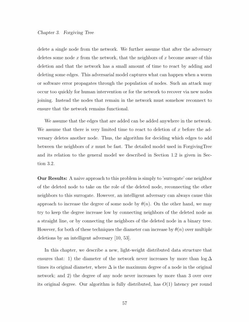
Chapter 3. Forgiving Tree
delete a single node from the network. We further assume that after the adversary
deletes some node x from the network, that the neighbors of x become aware of this
deletion and that the network has a small amount of time to react by adding and
deleting some edges. This adversarial model captures what can happen when a worm
or software error propagates through the population of nodes. Such an attack may
occur too quickly for human intervention or for the network to recover via new nodes
joining. Instead the nodes that remain in the network must somehow reconnect to
ensure that the network remains functional.
We assume that the edges that are added can be added anywhere in the network.
We assume that there is very limited time to react to deletion of x before the ad-
versary deletes another node. Thus, the algorithm for deciding which edges to add
between the neighbors of x must be fast. The detailed model used in ForgivingTree
and its relation to the general model we described in Section 1.2 is given in Sec-
tion 3.2.
Our Results: A naive approach to this problem is simply to ’surrogate’ one neighbor
of the deleted node to take on the role of the deleted node, reconnecting the other
neighbors to this surrogate. However, an intelligent adversary can always cause this
approach to increase the degree of some node by θ(n). On the other hand, we may
try to keep the degree increase low by connecting neighbors of the deleted node as
a straight line, or by connecting the neighbors of the deleted node in a binary tree.
However, for both of these techniques the diameter can increase by θ(n) over multiple
deletions by an intelligent adversary [10, 53].
In this chapter, we describe a new, light-weight distributed data structure that
ensures that: 1) the diameter of the network never increases by more than log ∆
times its original diameter, where ∆ is the maximum degree of a node in the original
network; and 2) the degree of any node never increases by more than 3 over over
its original degree. Our algorithm is fully distributed, has O(1) latency per round
57

Chapter 3. Forgiving Tree
and requires each node to send and receive O(1) messages per round. The formal
statement and proof of these results is in Section 4.7.1. Moreover, we show (in
Section 4.7.2) that in a sense our algorithm is asymptotically optimal, since any
algorithm that increases node degrees by no more than a constant must, in some
cases, cause the diameter of a graph to increase by a log ∆ factor.
The algorithm requires a one-time setup phase to do the following two tasks.
First, we must find a breadth first spanning tree of the original network rooted at an
arbitrary node. In the synchnronous communication model, this can be done with
latency equal to the diameter of the original network, and, with high probability,
each node v sending O(log n) messages along every edge incident to v, as in the
algorithm due to Cohen [11]. The second task required is to set up a simple data
structure for each node that we refer to as a will. This will, which we will describe
in detail in the Section 3.3, gives instructions for each node v on how the children
of v should reestablish connectivity if v is deleted. Creating the will requires O(1)
messages to be sent along the parent and children edges of the global breadth-first
search tree created in the first task.
Related Work:
In this chapter, we build on earlier work in [10, 53].
There have been numerous papers on dealing with adversarial atttacks in net-
works. Kuhn et al [37, 38] describe efficient algorithms that provably ensure that
node degree and network diameter stay small even in the case where an adversary can
either add or delete up to a fixed number of nodes in any time step. They describe
algorithms for the hypercube [38] and pancake topology [37] and suggest how their
approach can apply to any recursively defined peer-to-peer topology. In contrast, our
algorithm does not handle adversarial insertions, but it is immediately applicable to
any arbitrary reconfigurable network, even those that are not recursively defined.
58

Chapter 3. Forgiving Tree
3.2 Delete and Repair Model
We now describe the details of our delete and repair model. Let G = G0 be an
arbitrary graph on n nodes, which represent processors in a distributed network.
One by one, the Adversary deletes nodes until none are left. After each deletion,
the Player gets to add some new edges to the graph, as well as deleting old ones.
The Player’s goal is to maintain connectivity in the network, keeping the diameter
of the graph small. At the same time, the Player wants to minimize the resources
spent on this task, in the form of extra edges added to the graph, and also in terms
of the number of connections maintained by each node at any one time (the degree
increase). We seek an algorithm which gives performance guarantees under these
metrics for each of the n! possible deletion orders.
Unfortunately, the above model still does not capture the behaviour we want,
since it allows for a centralized Player who ignores the structure of the original
graph, and simply installs and maintains a complete binary tree, using a leaf node
to substitute for each deleted node.
To avoid this sort of solution, we require a distributed algorithm which can be
run by a processor at each node. Initially, each processor only knows its neighbors
in G0, and is unaware of the structure of the rest of the G0. After each deletion
(forming Ht), only the neighbors of the deleted vertex are informed that the deletion
has occurred. After this, processors are allowed to communicate by sending a limited
number of messages to their direct neighbors. We assume that these messages are
always sent and received successfully. The processors may also request new edges
be added to the graph to form Gt. The only synchronicity assumption we make is
that the next vertex is not deleted until the end of this round of computation and
communication has concluded. To make this assumption more reasonable, the per-
node communication should be O(log n) bits, and should moreover be parallelizable
59

Chapter 3. Forgiving Tree
so that the entire protocol can be completed in O(1) time if we assume synchronous
communication.
We also allow a certain amount of pre-processing to be done before the first
deletion occurs. This may, for instance, be used by the processors to gather some
topological information about G0, or perhaps to coordinate a strategy. Another
success metric is the amount of computation and communication needed during this
preprocessing round. Our full model is described as Model 3.2.1.
This model can be seen as a special case of our general model (Section 1.2). We
assume we begin with a connected graph of n vertices and do not explicitly discuss
node insertions in ForgivingTree. Since only deletions happen, n can only decrease.
For this reason, for our bounds, we need only compare our graph properties in the
present graph at timestep t (Gt), to the initial graph G0 which has n vertices.
3.3 The Forgiving Tree algorithm
At a high level, our algorithm works as follows. We begin with a rooted spanning
tree T , which without loss of generality may as well be the entire network.
Each time a non-leaf node v is deleted, we think of it as being replaced by a
balanced binary tree of “virtual nodes,” with the leaves of the virtual tree taking
v’s place as the parents of v’s children. Depending on certain conditions explained
later, the root of this “virtual tree” or another virtual node (known as v’s heir—this
will be discussed later) takes v’s place as the child of v’s parent. This is illustrated
in figure 4.5. Note that each of the virtual nodes which was added is of degree 3,
except the heir, if present.
When a leaf node is deleted, we do not replace it. However, if the parent of the
deleted leaf node was a virtual node, its degree has now reduced from 3 to 2, at
60

Chapter 3. Forgiving Tree
Each node of G0 is a processor.
Each processor starts with a list of its neighbors in G0.
Pre-processing: Processors may send messages to and from their neighbors.
for t := 1 to n do
Adversary deletes a node vt from Gt−1, forming Ht.
All neighbors of vt are informed of the deletion.
Recovery phase:
Nodes of Ht may communicate (in parallel) with their immediate neighbors.
These messages are never lost or corrupted, and may contain the names of other
vertices.
During this phase, each node may insert edges joining it to any other nodes as
desired. Nodes may also drop edges from previous rounds if no longer required.
At the end of this phase, we call the graph Gt.
end for
Success metrics: Minimize the following “complexity” measures:
1. Degree increase. maxt<n
maxv
degree(v,Gt)− degree(v,G0)
2. Diameter stretch. maxt<n
diam(Gt)/diam(G0)
3. Communication per node. The maximum number of bits sent by a single
node in a single recovery round.
4. Recovery time. The maximum total time for a recover round, assuming
it takes 1 bit no more than 1 time unit to traverse any edge and unlimited
local computational power at each node.
Model 3.2.1: The Delete and Repair Model – Distributed View.
61

Chapter 3. Forgiving Tree
dda b f g hc e
v
P
bd
ef
g
h
P
ca
ba c e g hf
Figure 3.1: Deleted node v replaced by its Reconstruction Tree. The nodes in theoval are helper nodes. Regular helper nodes are depicted by circles and the heirhelper node by a rectangle.
which point we consider it redundant and “short-circuit” it, removing it from the
graph, and connecting its surviving child directly to its parent. This helps to ensure
that, except for heirs, every virtual node is of degree exactly 3.
After a long sequence of such deletions, we are left with a tree which is a patchwork
mix of virtual nodes and original nodes. We note that the degrees of the original
nodes never increase during the above procedure. Also, because the virtual trees are
balanced binary trees, the deletion of a node v can, at worst, cause the distances
between its neighbors to increase from 2 to 2dlog de, where d is the degree of v. This
ensures that, even after an arbitrary sequence of deletions, the distance between any
pair of surviving actual nodes has not increased by more than a dlog ∆e factor, where
∆ is the maximum degree of the original tree.
Since our algorithm is only allowed to add edges and not nodes, we cannot really
add these virtual nodes to the network. We get around this by assigning each virtual
node to an actual node, and adding new edges between actual nodes in order to
allow “simulation” of each virtual node. More precisely, our actual graph is the
homomorphic image of the tree described above, under a graph homomorphism which
fixes the actual nodes in the tree and maps each virtual node to a distinct actual
node which is “simulating” it. The existence of such a mapping is a consequence of
62

Chapter 3. Forgiving Tree
the fact that all the virtual nodes have degree 3, except heirs, which have degree 2
(and there are not too many of these), and will be proved later. Note that, because
each actual node ever simulates at most one virtual node at a time, and virtual
nodes have degree at most 3, this ensures that the maximum degree increase of our
algorithm is at most 3.
The heart of our algorithm is a very efficient distributed algorithm for keeping
track of which actual node is assigned to simulate each virtual node, so that the
replacement of each deleted node by its virtual tree can be done in O(1) time. We
accomplish this using a system of “wills,” in which each vertex v instructs each of
its children (or their “heirs”) in the event of v’s deletion, how to simulate the virtual
tree replacing v, and also the virtual node v was simulating (if any).
This will is prepared in advance, before v’s deletion, and entrusted to v’s children
or their surviving heirs. An example of this is shown in figure 3.2. Certain events,
such as the deletion of one of v’s children, or a change in which virtual node v is
simulating, may cause v to revise its will, informing the affected children or their
surviving heirs. As shall be seen, the total number of messages and node IDs which
must be sent is O(1) per deleted vertex; the number of bits sent is thus O(log n).
In addition, there is a startup cost for communicating the initial wills: this is O(1)
latency; and O(1) messages and O(log n) bits per edge in the original network.
3.3.1 Distributed implementation
To begin with, in Table 4.1 we list the data kept by each real node v required for
the ForgivingTree algorithm. We have four main classes of fields, according to the
way they are used by the node. ‘Current fields’ give a node’s present configuration
and status in the tree. ‘Reconstruction fields’ hold the data needed for a node to
reconstruct connections when one of its neighbors gets deleted. ‘Helper fields’ hold
63

Chapter 3. Forgiving Tree
information with regard to the helper node being simulated by this node. Each
node also stores some special flags with regard to its helper or heir status. In the
description that follows, we shall refer directly to these fields.
Current fields Fields having information about a node’s current neigh-bors.
parent(v) Parent of v.children(v) Children of v.SubRT(v) Stores the Reconstruction Tree (RT) of v minus a pos-
sible helper node simulated by heir(v). This tree ofhelper and real nodes shall replace v if v is deleted.
heir(v) The heir of v.Helper fields Fields specifying a node’s role as a helper node.hparent(v) Parent of the helper node v may be simulating.hchildren(v) Children of the helper node v may be simulating.Reconstruction fields Fields used by a node to reconstruct its connections
when its neighbor is deleted.nextparent(v) The node which will be the next parent of v.nexthparent(v) The node which will be the next hparent of v.nexthchildren(v) The node(s) which will be the next hchildren of v.Flags Specifying a node’s helper or heir status.ishelper(v) (boolean field). True if v is simulating a helper node,
false otherwise.isreadyheir(v) (boolean field). True if v is simulating an heir in ready
state, false otherwise (wait or deployed state).
Table 3.1: The fields maintained by a node v
At the top level, our algorithm is specified as Algorithm 4.5.1 : Forgiving tree.
Algorithm 4.5.1 uses Algorithms 2 to 9, which will be described at the appropriate
places. As referred to earlier, Forgiving tree works on a tree which may be
obtained from the original graph during a preprocessing phase. The next stage is an
initialisation phase in which the appropriate data structures are setup. Once these
are setup, the network is ready to face the adversarial attacks as and when they
happen.
64

Chapter 3. Forgiving Tree
h
h
RT(x)
p
a b
ab
c h
c
PP
h.hnextparent=p
c
p
x
a b h b
a
h
c
b
h
p
a
a
b
b
nextparent: c
nexthparent: p
nexthchildren: b
nextparent: a
nexthparent: b
nexthchildren: a,b
nextparent: a
c
c
h
ba
h
b
c
c
nexthparent: h
nexthchildren: a,c
nextparent: c
nexthparent: b
nexthchildren: c,h
h
a
a
b
a
c
c
Figure 3.2: The leftmost column shows a small segment of the network. The RT(x)corresponding to this figure is shown. Every neighbor of node x stores the portionof RT(x) relevant to it. Each rectangular box is labelled with a neighbor and showsthe portions and the value of the corresponding fields .
The Initialization phase
This phase is specified in Algorithm 4.5.2 : Init(). We assume each node v has a
unique identification number which we call ID(v). Every node in the tree initializes
the fields we have listed in Table 4.1. In our descriptions if no data is available or
appropriate for a field, we set it to EMPTY. Since no deletion has happened yet
and there are no helper nodes in the system, the helper fields are set to EMPTY.
The current fields parent(v) and children(v) are assigned pointers to the parent and
children of v. Of course, if v is a leaf node children(v) is EMPTY and if v is the root
of the tree parent(v) is EMPTY.
As stated earlier, the heart of our algorithm is the system of wills created by
nodes and distributed among its neighbors. The will of a node, v, has two parts:
firstly, a Reconstruction Tree (SubRT(v)), which will replace v when it is deleted by
65

Chapter 3. Forgiving Tree
m n o
m n o
r
j
p
i k
g
h
fca
b d
e
a gfedcb
h
r
v
c
j
p
ab
d e
i k
gf
h
gc e
m n o
h
p
ga
ji k
fedcb
r
i
i j
k
r
k
hj
h
fa
b d
a gfedcb
m n o
m n o
ga hfedcb
r
i j k
g
h
fea
b
a
c
gfeb
k
r
i
ih
j
j k
c
m n o
hb c ga fe
r
i j k
m n o
io
j
e
j k
gfe
f gab
a b
c
i
c
k
r
n o
m
m
n
self healing. The network after all the deletions and
om n
r
fe gc
j
a b
ki
.
.
Turn 1: Adversary deletes v. Vertices a through h take over helper nodes in RT(v).h is v’s heir and connectsthe real graph now contains a
Turn 2: Adversary
deletes p. Vertices h, i, j, and k take over helpernodes in RT(p). h takes over the helperi. k is p’s heir and connects to both h and parent(p)
Turn 3: Adversary deletes d. The original helper node of c is made
nodes formerly held by d.
Turn 4: Adversary deletes h. Vertices m, n and o take over helper nodes
Note that since the number of children of h was not a power of 2, not all the leaves of RT(h) are at the same depth.
cycle, (b, c, d)
redundant by the deletion of d and so is
of RT(h). o is heir of h and takes over h’s
bypassed. c takes over the helper
to both p and q. Note that
role of v in RT(p). d attaches to
and takes over h’s helper role.
Figure 3.3: An illustrative sequence of deletions and healings.
66

Chapter 3. Forgiving Tree
the Adversary, and secondly, the delegation of v’s helper responsibilities (if any) to
a child node, heir(v). For concreteness, we initially designate the child of v with the
highest ID as heir(v). In the event that heir(v) is deleted, its role will be taken over
by its heir, if any. If heir(v) is a leaf when it is deleted, then v will designate its new
heir to be the surviving child whose helper node has just decreased in degree from 3
to 2.
Algorithm 3.3.5: GenerateSubRT computes SubRT(v). If the node v has
no helper responsibilities, as is during this phase, RT(v) is simply SubRT(v) with a
helper node simulated by heir(v) appended on as the parent of the root of SubRT(v).
Figure 4.5 and Turn 1 in Fig 3.3 depict such Reconstruction Trees. If the node v has
helper responsibilities RT(v) is the same as SubRT(v). Node v uses Algorithm 3.3.5
to compute SubRT(v) as follows: All the children of v are arranged as a single layer
in sorted (say, ascending) order of their IDs. Then a set of helper nodes - one node
for each of the children of v except the heir are arranged above this layer so as to
construct a balanced binary search tree ordered on their IDs.
The last step of the initialization process is to finalize the will and transmit it to
the children. Each child is given only the portion of the will relevant to it. Thus,
only this portion needs to be updated whenever a will changes. The division of RT
into these portions is shown in figure 3.2. There are fundamentally two different
kinds of wills : one prepared by leaf nodes who have helper responsibilities and the
other by non-leaf nodes. Obviously, during the initialization phase, only the second
kind of will is needed. This is finalized and distributed as shown in Algorithm
3.3.6: MakeWill. The children of v initialize their reconstruction fields with the
values from SubRT(v). If later v gets deleted these values will be copied to present
and helper fields such that RT(v) is instantiated. Notice that the role the heir will
assume is decided according to whether v is a helper node or not. Since v cannot be
a helper node in this phase, the heir node simply sets its reconstruction fields so as
67

Chapter 3. Forgiving Tree
to be between the root of SubRT(v) and parent(v). In this case when RT(v) will be
instantiated, the helper node simulated by heir(v) shall have only one child: we will
say that heir(v) is in the ready phase (explained later) and set the flag isreadyheir(v)
to true. In the initialization phase both the isreadyheir and ishelper flags will be set
to false.
This completes the setup and initialization of the data structure. Now our net-
work is ready to handle adversarial attacks. In the context of our algorithm, there
are two main events that can happen repeatedly and need to be handled differently:
Deletion of an internal node
The healing that happens on deletion of a non-leaf node is specified in Algorithm
4.5.3: FixNodeDeletion. In our model, we assume that the failure of a node is
only detected by its neighbors in the tree, and it is these nodes which will carry out
the healing process and update the changes wherever required. If the node v was
deleted, the first step in the reconstruction process is to put RT into place according
to Algorithm 4.5.8: makeRT. Note that all children of v have lost their parent. Let
us discuss the reconstruction performed by non-heir nodes first. They make an edge
to their new parent (pointer to which was available as nextparent()) and set their
current fields. Then they take the role of the helper nodes as specified in RT(v) and
Algorithm 3.3.9: MakeHelper and make the required edges and field changes to
instantiate RT(v).
To understand what the heir node does in this case, it will be useful here to have
a small discussion on the states of a regular/heir node:
States of a heir/regular node: Consider a node v and its heir h. From the point
of view of h, we can imagine h to be in one of three states which we call wait, ready
68

Chapter 3. Forgiving Tree
READY
WAIT DEPLOYED
Figure 3.4: The states of a node with respect to helper duties: Waiting, Ready andDeployed
and deployed. These states are illustrated in figure 3.4. For ease of discussion, let
us call the helper node that a node is simulating helper(node). In brief, a node is
considered to be in the wait state when it has no helper responsibilities, in the ready
state when helper(node) with one child, and in the deployed state when helper(node)
has two children (which is the maximum possible). Notice that the node can be in
the wait state only when v has not been deleted and thus, h has assumed no helper
responsibilities. It only has the will of v and is in limbo with regard to helper duties.
Now consider the case when v gets deleted. Following are the possibilities:
• node v had no helper responsibilities : This happens when v’s original parent
was not deleted. Thus, v could be a regular child or a heir in the wait state.
On v’s deletion h moves to the ready state and sets its flag isreadyheir to
True. This is the state in which helper(h) has only one child i.e. the root of
SubRT(v). This happens when h executes its portion of the will of v using
Algorithm 4.5.8: makeRT. Note that this may not be the final state for the
helper node of h, and is thus called the ready state.
69

Chapter 3. Forgiving Tree
• node v had helper responsibilities : There are two further possibilities:
– helper(v) had one child : This can only happen when v was a heir node
in the ready state. Thus, v’s flags ishelper and isreadyheir were both set
to True. Node h will take over the helper responsibilities of v and thus,
in turn, h will now have one child i.e. will be in the ready state and will
set its flags ishelper and isreadyheir to True. Notice that if v was an heir,
h will now also take over those responsibilities, and on future deletions
of v’s ancestors could move further up the tree either as an heir in ready
state or in a deployed state become a full helper node.
– helper(v) had two children: Node v could be a regular child or heir. h
will fully take over the helper responsibilities of v, and thus helper(h)
shall acquire two children and move on to the deployed state. Notice that
previously h could have been in either wait or ready state. Since it is now
not in the ready state, it will set its isreadyheir flag to False and ishelper
flag to True.
It is easy to see that a regular i.e. non-heir node can be in either wait or deployed
state.
Here we also define the following operation, which is used in Algorithms 3.3.4
and 4.5.8:
bypass(x): Precondition: |hchildren(x)| = 1 i.e the helper node has a single child.
Operation: Delete helper(x) i.e. hparent(x) and hchildren(x) remove their
edges with x and make a new edge between themselves.
hparent(x)← EMPTY; hchildren(x)← EMPTY.
70

Chapter 3. Forgiving Tree
We can now easily see how the heir of v, h takes part in the reconstruction
according to Algorithm 4.5.8: makeRT. Node h can be either in wait state or ready
state. If it is in the wait state it simply takes its helper responsibilities according
to Algorithm 3.3.9: MakeHelper, as in turn 1 of figure 3.3 . Note that here h
checks if it has moved to the ready state and sets its isreadyheir flag accordingly.
If h was already in ready state, it relinquishes its present helper role and moves on
to the new helper role. To relinquish its present role, node h intimates hparent(h)
and hchildren(h), and together they accomplish this as specified by the operation
bypass(h). Turn 2 in Fig 3.3 illustrates this.
Once RT(v) is in a place, there may be a need for the parent of v to recompute
its will. This happens only when v did not already have a helper role or equivalently
when heir(v) moves to a ready state. Lines 2 to 6 of Algorithm 4.5.3 deals with this
situation. Node parent(v) simply replaces v by heir(v) in its will and retransmits it.
At the end of this healing process, the children of the deleted nodes check if they
need to leave the second kind of will, which we call a LeafWill. This will is required
only for those nodes which are leaves in our tree and have virtual responsibilities.
Since they have no children to take over their helper responsibilities they leave this
responsibility to their parent. We will discuss this in greater detail in the next
section.
Deletion of a leaf node
If the adversary removes a leaf node from the system, the healing is accomplished
by its neighbors as specified in Algorithm 3.3.4: FixLeafDeletion. Let v be the
deleted leaf node and p be its parent. Let us consider the simple case first. This
is when the deleted node had no helper responsibility. This also implies its original
parent did not suffer a deletion. Node p simply removes v from the list of its children
and then recomputes and redistributes its will.
71
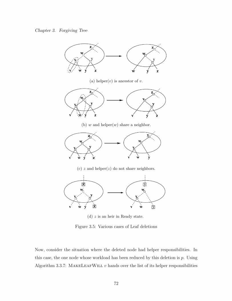
Chapter 3. Forgiving Tree
(a) helper(v) is ancestor of v.
(b) w and helper(w) share a neighbor.
(c) z and helper(z) do not share neighbors.
(d) z is an heir in Ready state.
Figure 3.5: Various cases of Leaf deletions
Now, consider the situation where the deleted node had helper responsibilities. In
this case, the one node whose workload has been reduced by this deletion is p. Using
Algorithm 3.3.7: MakeLeafWill v hands over the list of its helper responsibilities
72

Chapter 3. Forgiving Tree
to p. Here, a special case may arise when v is simulating a helper node which has
v itself as one of its hchildren. Recall that parent(v) is v’s ancestor closest to v
in the tree. This implies that parent(v) = hparent(v) = p. The only thing that
p needs to do if v is deleted is to remove v from its hchildren and add itself (for
consistency). This is the will conveyed by v to p. When v is deleted, p simply
updates its helper fields. For other cases, v simply sends its helper fields to p to be
copied to p’s helper reconstruction fields. In this situation, when v is actually deleted
the following happens: the helper node that p is simulating is deleted and bypassed
by the bypass operation defined earlier. Node p now simulates a new helper node
that has the same helper responsibilities previously fulfilled by v. In case the deleted
leaf node was itself an heir in ready state, p detects this and sets its flags accordingly.
Again at the end of the reconstruction, the leaf nodes reconstruct their wills. An
example of such a leaf deletion is the deletion of node d at Turn 3 as shown in figure
3.3.
Important Note: When implementing the pseudocode for Algorithm 3.3.6
(MakeWill), it is important to bear in mind that when RT(v) is being updated
due to a node deletion, most of SubRT(v) will be unchanged. In fact, only O(1)
nodes will need to have their fields updated. These can be found and updated more
efficiently by a more detailed algorithm based on case analysis.
73

Chapter 3. Forgiving Tree
3.4 Results
3.4.1 Upper Bounds
Before considering the main theorem, we shall prove a couple of lemmas.
Lemma 3.1. In the Forgiving Tree, a real node can simulate at most one helper node
at a time.
Proof. A node simulates a new helper node if and only if its parent is deleted (Sec-
tion 3.3.1) or a sibling that is a leaf node in the Forgiving Tree is deleted (Sec-
tion 3.3.1). We will show that whenever either of the above events happens and the
node has to simulate a new helper node, it no longer needs to simulate the helper
node it was simulating prior to these events occuring and thus it always simulates at
most one helper node at a time. Let us consider the cases in more detail. Consider
a node v and it’s parent node p.
• Parent node p is deleted: There are three possibilities:
– Node v is in Wait state (i.e. no previous helper role): Node v will now take
over the role of exactly one helper node as specified for RT(p) (Figure 4.5).
– Node v is in Ready heir: Node v will remove its previous helper node
using operation bypass(v), and be redeployed in the Ready state or as a
Deployed node (Figure 3.4). An example is node h at turn 2 in Figure 3.3.
– Node v is in Deployed state: By construction and by definition of parent in
the Forgiving Tree (Line 4, Algorithm 3.3.6:MakeWill), p is the parent
of v through helper(p). This implies that v’s parent in the Forgiving Tree
is helper(p) (not p itself). Thus v does not feature in the will of p and will
not simulate a new helper node on deletion of p.
74
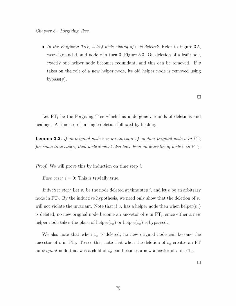
Chapter 3. Forgiving Tree
• In the Forgiving Tree, a leaf node sibling of v is deleted: Refer to Figure 3.5,
cases b,c and d, and node c in turn 3, Figure 3.3. On deletion of a leaf node,
exactly one helper node becomes redundant, and this can be removed. If v
takes on the role of a new helper node, its old helper node is removed using
bypass(v).
Let FTi be the Forgiving Tree which has undergone i rounds of deletions and
healings. A time step is a single deletion followed by healing.
Lemma 3.2. If an original node x is an ancestor of another original node v in FTi
for some time step i, then node x must also have been an ancestor of node v in FT0.
Proof. We will prove this by induction on time step i.
Base case: i = 0: This is trivially true.
Inductive step: Let vx be the node deleted at time step i, and let v be an arbitrary
node in FTi. By the inductive hypothesis, we need only show that the deletion of vx
will not violate the invariant. Note that if vx has a helper node then when helper(vx)
is deleted, no new original node become an ancestor of v in FTi, since either a new
helper node takes the place of helper(vx) or helper(vx) is bypassed.
We also note that when vx is deleted, no new original node can become the
ancestor of v in FTi. To see this, note that when the deletion of vx creates an RT
no original node that was a child of vx can becomes a new ancestor of v in FTi.
75

Chapter 3. Forgiving Tree
Let ∆ be its maximum degree of a node in FT0.
Lemma 3.3. Let danci(v) be the number of ancestors of v in FT0 that have been
deleted by time step i.
For all nodes v,
depthi(v) ≤ depth0(v) + log ∆× danci(v)
Proof. We shall prove this by induction on time i.
Base case: i = 0: This is trivial since there have been no deletions so far.
Inductive step: Let vi be the node deleted at the ith deletion. Consider an
arbitrary original node v in FTi. First, observe that the removal of helper(vi), if it
exists (helper(vi) will be removed on deletion of node vi), never increases the depth
of any node. This is because the helper node is either replaced by another helper
node or it is removed in the bypass operation, which will never increase the depth of
any node. We now consider the deletion of the original node vi. There are two cases
for node v:
• Node v is not in the subtree rooted at vi: Here,
depthi(v) ≤ depthi−1(v) and thus the induction holds.
• Node v is in the subtree rooted at vi: By lemma 3.2, node vi must have been
an ancestor of v in FT0. Since Algorithm 4.5.3 replaces vi with RT(vi), which
is a balanced binary tree, we know that,
depthi(v) ≤ depthi−1(v) + log ∆
Also, by the Inductive hypothesis,
depthi−1(v) ≤ depth0(v) + log ∆× danci−1(v)
76

Chapter 3. Forgiving Tree
These two equations imply that
depthi(v) ≤ depth0(v) + log ∆× danci−1(v) + log ∆
≤ depth0(v) + log ∆× danci(v)
Now, we prove our main theorem. Let FT0 be the original tree, and let D be its
diameter.
Theorem 3.1. The Forgiving Tree has the following properties:
1. The Forgiving Tree increases the degree of any vertex by at most 3.
2. The Forgiving Tree always has diameter O(D log ∆).
3. The latency per deletion and number of messages sent per node per deletion is
O(1); each message contains O(1) node IDs and thus O(log n) bits.
Proof. Parts 1 and 3 follow directly by construction of our algorithm. For part 1,
we note that for a node v, any degree increase for v is imposed by its edges to
hparent(v) and hchildren(v). By lemma 3.1, node v can play the role of at most one
helper node at any time and the number of hchildren is never more than 2, because
the reconstruction trees are binary trees. Thus the total degree increase is at most 3.
Part 3 also follows directly by the construction of our algorithm, noting that, because
the virtual nodes all have degree at most 3, healing one deletion results in at most
O(1) changes to the edges in each affected reconstruction tree. In fact, the changes
to RT(w) for an affected node w do not require new information, which allows these
messages to be computed and distributed in parallel.
77

Chapter 3. Forgiving Tree
We next show Part 2, that the diameter of the Forgiving Tree is always O(D log ∆).
Consider the Forgiving Trees FT0 and FTi. Let their respective heights be h and hi.
Consider a node x in FTi which has the maximum depth, equal to hi. By lemma 3.3,
hi ≤ depth0(x) + log ∆× danci(x)
≤ h + log ∆× danci(x)
Since, node x can have at most h ancestors,
hi ≤ h + log ∆× h
≤ log ∆× (h+ 1)
Since the diameter of a tree can at most be twice the height of the tree, the
diameter of FTi is at most 2(h + 1) log ∆, or O(D log ∆).
3.4.2 Lower Bounds
Theorem 3.2. Consider any self-healing algorithm that ensures that: 1) each node
increases its degree by at most α, for some α ≥ 3; and 2) the diameter of the graph
increases by a multiplicative factor of at most β. Then for any positive ∆, for some
initial graph with maximum degree ∆, it must be the case that β ≥ 12[logα+1 ∆− 1].
Proof. Let G be a star on ∆ + 1 vertices, where x is the root node, and x has ∆
edges with each of the other nodes in the graph. Let G′ be the graph created after
the adversary deletes the node x. Consider a breadth first search tree, T , rooted at
some arbitrary node y in G′. We know that the self-healing algorithm can increase
the degree of each node by at most α, thus the root node in T can have at most α+1
78

Chapter 3. Forgiving Tree
α + 1
Degree(v) =
y
α
Δx
y
Figure 3.6: Deletion of the central node v of a star leads to an increase in thediameter. Here, the healing algorithm increases the degree of any node by at mostα.
children, and other nodes can have at most α children. Let h be the height of T .
Then we know that 1 + (α + 1)∑h−1
i=0 αi ≥ ∆. This implies that (α + 1)h+1 ≥ ∆ for
α ≥ 3, or h+ 1 ≥ logα+1 ∆. Since the diameter of G is 2, we know that β ≥ h/2, and
thus 2β+ 1 ≥ logα+1 ∆. Rearranging, we get β ≥ 12[logα+1 ∆− 1]. This is illustrated
in figure 3.6.
We note that this lower-bound compares favorable with the general result achieved
with our data structure. The Forgiving Tree can be modified so that it ensures that
1) the degree of any node increases by no more than α for any α ≥ 3; and that the
diameter increases by no more than a multiplicative factor of β ≤ 2 logα ∆ + 2.
3.5 Conclusion
In this chapter, we have presented a distributed data structure that withstands
repeated adversarial node deletions by adding a small number of new edges after each
deletion. Our data structure ensures two key properties, even when up to all nodes
in the network have been deleted. First, the diameter of the network never increases
by more than O(log ∆) times its original diameter, where ∆ is the maximum original
79

Chapter 3. Forgiving Tree
degree of any node. For many peer-to-peer systems, ∆ is at most polylogarithmic,
and so the diameter would increase by no more than a O(log log n) multiplicative
factor. Second, no node ever increases its degree by more than 3 over its original
degree.
Several open problems remain. For example, how do we extend our model and
algorithm to handle insertions of nodes and multiple deletions? Can we protect
other invariants? Can we extend our distributed data structure to ensure that the
stretch between any pair of nodes increases by no more than a certain amount? Can
we design our algorithms so they can work directly on graphs instead of spanning
trees of those graphs? We have some preliminary positive results answering the
above questions that build on this work. We can also consider extending self-healing
beyond our present model. For example, Can we design algorithms for less flexible
networks such as sensor networks? Can we extend the concept of self-healing to other
objects besides graphs? For example, can we design algorithms to rewire a circuit so
that it maintains its functionality even when multiple gates fail? Can our approach
be used to better understand self-healing in biological systems such as the human
brain?
80

Chapter 3. Forgiving Tree
1: Given a tree T (V,E)
2: Init(T).
3: while true do
4: if a vertex x is deleted then
5: if children(x) is EMPTY then
6: FixLeafDeletion(x)
7: else
8: FixNodeDeletion(x)
9: end if
10: end if
11: end while
Algorithm 3.3.1: Forgiving tree: The main function.
Require: each node of T has a unique ID
1: for each node v ∈ T do
2: children(v)← children of v.
3: parent(v)← if v is root of T then EMPTY else parent of v.
4: isreadyheir(v)← false.
5: ishelper(v)← false.
6: hparent(v)← EMPTY.
7: hchildren(v)← EMPTY.
8: heir(v)← if v is a leaf node then EMPTY else child of v with highest ID.
9: SubRT(v)← generateSubRT(v).
10: MakeWill(v, SubRT(v)).
11: end for
Algorithm 3.3.2: Init(T): initialization of the Tree T
81

Chapter 3. Forgiving Tree
1: MakeRT(children(v), parent(v)).
2: let h = heir(v).Let p = parent(v)
3: if isreadyheir(h) = true then
4: hparent(h) replaces v by h in SubRT(hparent(h)).
5: MakeWill(hparent(h), SubRT(hparent(h))).
6: end if
7: for each node y ∈ children(v) do
8: if children(y) is EMPTY then
9: MakeLeafWill(y).
10: end if
11: end for
Algorithm 3.3.3: FixNodeDeletion(v): Self-healing on deletion of internal node
82

Chapter 3. Forgiving Tree
1: let p = parent(v)
2: if ishelper(p) = false then
3: p removes v from children(p)
4: SubRT (p)← GenerateSubRT(p)
5: MakeWill(p)
6: else
7: Let z = parent(v).
8: if z 6= hparent(v) then
9: bypass(z).
10: end if
11: z makes edges with nexthparent(z),nexthchildren(z).
12: hparent(z)← nexthparent(z).
13: hchildren(z)← nexthchildren(z).
14: if |hchildren(z)|=1 then
15: isreadyheir(z) = true
16: end if
17: end if
18: for each node y ∈ children(v) do
19: if children(y) is EMPTY then
20: MakeLeafWill(y).
21: end if
22: end for
Algorithm 3.3.4: FixLeafDeletion(v): Self-healing on deletion of leaf node
83

Chapter 3. Forgiving Tree
1: Let Lset be a set of vertices representing all members of children(v), and Iset be
another set of vertices. representing all members of children(v) except the one
with the highest ID.
2: Arrange Lset in ascending order of their IDs.
3: Using the arranged Lset as leaves and Iset as the internal nodes construct a
Balanced Binary Search Tree SubRT ordered on the nodes ID.
4: return SubRT
Algorithm 3.3.5: GenerateSubRT(v): Computes the Reconstruction Tree (RT)
of v minus a possible helper node simulated by heir(v).
84

Chapter 3. Forgiving Tree
1: Let p = parent(v). Let rv be root of SubRT(v).
2: for each node y ∈ children(v) do
3: let ly be the leaf vertex representing y in SubRT(v). Let hy be the internal
node in SubRT representing y.
4: If hy is ly’s parent in SubRT(v) then nextparent(y)← parent of hy in SubRT
else nextparent(y)← parent of ly in SubRT.
5: if y 6= heir(v) then
6: nexthchildren(y)← children of hy in SubRT.
7: nexthparent(y)← parent of hy in SubRT.
8: else
9: if ishelper(v) = true then
10: nexthchildren(y)← hchildren(v).
11: nexthparent(y)← hparent(v).
12: nexthparent(rv)← p.
13: else
14: nexthchildren(y)← rv.
15: nexthparent(y)← p.
16: nexthparent(rv)← y.
17: end if
18: end if
19: end for
Algorithm 3.3.6: MakeWill(v, SubRT(v)): Makes and distributes the will of v
85

Chapter 3. Forgiving Tree
1: let z = parent(v).
2: if z = hparent(v) then
3: nexthparent(z)← hparent(v).
4: nexthchildren(z)← hchildren(z)/v ∪ z. // z will take on itself as a child
of its helper node.
5: else
6: nexthparent(z)← hparent(v).
7: nexthchildren(z)← hchildren(v).
8: end if
Algorithm 3.3.7: MakeLeafWill(v): Leaf node leaves a will for its parent.
1: for each node x ∈ children(v) do
2: if isreadyheir(x) = true then
3: bypass(x). // hparent(x) and hchildren(x) bypass x and connect them-
selves.
4: MakeHelper(x).
5: else
6: x makes edge between itself and nextparent(x).
7: parent(x)← nextparent(x).
8: MakeHelper(x).
9: end if
10: end for
Algorithm 3.3.8: makeRT(children(v),parent(v)): Replace the deleted node
by its RT
86

Chapter 3. Forgiving Tree
1: v makes edges between itself and nexthchildren(v), and nexthparent(v).
2: hparent(v)← nexthparent(v).
3: hchildren(v)← nexthchildren(v).
4: ishelper(v) = true.
5: if |hchildren(v)| = 1 then
6: isreadyheir(v) = true. // Only an ’unemployed’ heir has a single child.
7: end if
Algorithm 3.3.9: MakeHelper(v): v takes over helper node responsibilities
87

Chapter 4
Forgiving Graph
The weak can never forgive.
Forgiveness is the attribute of the
strong.
Mahatma Gandhi.
In this chapter, we present the final of our algorithms discussed in this Disser-
tation. To recap, we consider the problem of self-healing in peer-to-peer networks
that are under repeated attack by an omniscient adversary. Here, we will assume
that, over a sequence of rounds, an adversary either inserts a node with arbitrary
connections or deletes an arbitrary node from the network. The network responds
to each such change by quick “repairs,” which consist of adding or deleting a small
number of edges.
These repairs essentially preserve closeness of nodes after adversarial deletions,
without increasing node degrees by too much, in the following sense. At any point
in the algorithm, nodes v and w whose distance would have been ` in the graph
formed by considering only the adversarial insertions (not the adversarial deletions),
will be at distance at most ` log n in the actual graph, where n is the total number of
88

Chapter 4. Forgiving Graph
vertices seen so far. Similarly, at any point, a node v whose degree would have been
d in the graph with adversarial insertions only, will have degree at most 3d in the
actual graph. Our distributed data structure, which we call the Forgiving Graph,
has low latency and bandwidth requirements.
The Forgiving Graph improves on the Forgiving Tree distributed data structure
from Chapter 3, [24], in the following ways: 1) it ensures low stretch over all pairs of
nodes, while the Forgiving Tree only ensures low diameter increase; 2) it handles both
node insertions and deletions, while the Forgiving Tree only handles deletions; 3) it
does not require an initialization phase, while the Forgiving Tree initially requires
construction of a spanning tree of the network.
4.1 Introduction
In Chapter 1, we have made case for the need of using responsive approaches in
reconfigurable networks for maintaining robustness and self-healing in networks. In
this chapter, we describe a distributed data structure for maintaining invariants in
a reconfigurable network. We note that our approach is responsive in the sense that
it responds to an attack by changing the network topology. Thus, it is orthogonal
and complementary to traditional non-responsive techniques for ensuring network
robustness.
This work builds significantly on results achieved in [24] (Presented in Chapter 3),
which presented a responsive, distributed data structure called the Forgiving Tree for
maintaining a reconfigurable network in the face of attack. Over a complete run of
Forgiving Tree: 1) The diameter of the network can never exceed its original diameter
by more than a multiplicative factor of O(log ∆) where ∆ is the maximum degree in
the graph; and 2) the total increase in the degree of any node can never be more than
3. The Forgiving Tree ensured two invariants: 1) the diameter of the network never
89

Chapter 4. Forgiving Graph
increased by more than a multiplicative factor of O(log ∆) where ∆ is the maximum
degree in the graph; and 2) the degree of a node never increased by more than an
additive factor of 3.
In the following pages, we present a new, improved distributed data structure
called the Forgiving Graph. The improvements of the Forgiving Graph over the For-
giving Tree are threefold. First, the Forgiving Graph maintains low stretch i.e. it
ensures that the distance between any pair of nodes v and w is close to what their
distance would be even if there were no node deletions. It ensures this property even
while keeping the degree increase of all nodes no more than a multiplicative fac-
tor of 3. Moreover, we show that this tradeoff between stretch and degree increase
is asymptotically optimal. Second, the Forgiving Graph handles both adversarial
insertions and deletions, while the Forgiving Tree could only handle adversarial dele-
tions (and no type of insertion). Finally, the Forgiving Graph does not require an
initialization phase, while the Forgiving Tree required an initialization phase which
involved sending O(n log n) messages, where n was the number of nodes initially in
the network, and had a latency equal to the initial diameter of the network. Ad-
ditionally, the Forgiving Graph is divergent technically from the Forgiving Tree, it
makes significant use of a novel distributed data structure that we call a Half-full
Tree or “haft”. hafts are discussed in Section 4.4. Our main algorithm is described
in Section 4.3 and Section 4.5.
Our Model: We remind the reader about the model we have been using in this
work. We assume that the network is initially a connected graph over n nodes.
An adversary repeatedly attacks the network. This adversary knows the network
topology and our algorithm, and it has the ability to delete arbitrary nodes from the
network or insert a new node in the system which it can connect to any subset of the
nodes currently in the system. However, we assume the adversary is constrained in
90

Chapter 4. Forgiving Graph
that in any time step it can only delete or insert a single node. The detailed model
is described in Section 4.2.
Our Results: For a peer-to-peer network that has both insertions and deletions,
let G′ be the graph consisting of the original nodes and inserted nodes without any
changes due to deletions. Let n be the number of nodes in G′. The Forgiving Graph
ensures that: 1) the distance between any two nodes of the actual network never
increases by more than log n times their distance in G′; and 2) the degree of any
node in the actual network never increases by more than 3 times its degree in G′.
Our algorithm is completely distributed and resource efficient. Specifically, after
deletion, repair takes O(log d log n) time and requires sending O(d log n) messages,
each of size O(log n) where d is the degree of the node that was deleted. The formal
statement and proof of these results is in Section 4.7.1.
Related Work: Our work significantly builds on work in [24] as described above.
Our model of attack and repair builds on earlier work in [10, 53] (The later is pre-
sented in Chapter 2).
4.2 Node Insert, Delete and Network Repair Model
We now describe the details of our node insert, delete and network repair model.
Let G = G0 be an arbitrary graph on n nodes, which represent processors in a
distributed network. In each step, the adversary either deletes or adds a node. After
each deletion, the algorithm gets to add some new edges to the graph, as well as
deleting old ones. At each insertion, the processors follow a protocol to update
their information. The algorithm’s goal is to maintain connectivity in the network,
keeping the distance between the nodes small. At the same time, the algorithm
91

Chapter 4. Forgiving Graph
wants to minimize the resources spent on this task, especially keeping node degree
small.
Initially, each processor only knows its neighbors in G0, and is unaware of the
structure of the rest of G0. After each deletion or insertion, only the neighbors of the
deleted or inserted vertex are informed that the deletion or insertion has occurred.
After this, processors are allowed to communicate by sending a limited number of
messages to their direct neighbors. We assume that these messages are always sent
and received successfully. The processors may also request new edges be added to
the graph. The only synchronicity assumption we make is that no other vertex is
deleted or inserted until the end of this round of computation and communication has
concluded. To make this assumption more reasonable, the per-node communication
cost should be very small in n (e.g. at most logarithmic).
We also allow a certain amount of pre-processing to be done before the first attack
occurs. This may, for instance, be used by the processors to gather some topological
information about G0, or perhaps to coordinate a strategy. Another success metric
is the amount of computation and communication needed during this preprocessing
round. Our full model is described in Figure 4.1.
For our success metrics, at any time T , we compare the actual graph GT to
the graph G′T which is the graph with only the original nodes (those at G0) and
insertions without regard to deletions and healing. This is the graph which would
have been present if the adversary was not doing any deletions and (thus) no self-
healing algorithm was active. This is the natural graph for comparing results. Notice
if there were no insertions happening in our model, we could have compared GT to
G0 but since insertions are happening, GT may not even have the same nodes as
G0 rendering a node-based comparison impossible. Figure 4.2 shows an example of
G′T and a corresponding GT . The figure also shows, in G′T , the nodes and edges
inserted and deleted, and in GT , the edges inserted by the healing algorithm, in
92

Chapter 4. Forgiving Graph
different colors, as the network evolved over time. Figure 4.3 shows how the two
graphs compare with regards to degree of a particular node v, and figure 4.4 shows
how the healing algorithm effects the distance between two nodes, u and v. Our
algorithm gaurantees our invariants on the ’complexity’ measures at every time step
that the algorithms is in execution.
93

Chapter 4. Forgiving Graph
Figure 4.1: The Node Insert, Delete and Network Repair Model – Distributed View.
Each node of G0 is a processor.Each processor starts with a list of its neighbors in G0.Pre-processing: Processors may exchange messages with their neighbors.for t := 1 to T do
Adversary deletes a node vt from Gt−1 or inserts a node vt into Gt−1, formingHt.if node vt is inserted thenvt and its new neighbors may update their information and exchange mes-sages with their neighbors.
end ifif node vt is deleted then
All neighbors of vt are informed of the deletion.Recovery phase:Nodes of Ht may communicate (asynchronously, in parallel) with their im-mediate neighbors. These messages are never lost or corrupted, and maycontain the names of other vertices.During this phase, each node may add edges joining it to any other nodesas desired. Nodes may also drop edges from previous rounds if no longerrequired.
end ifAt the end of this phase, we call the graph Gt.
end for
Success metrics: Minimize the following “complexity” measures:Consider the graph G′ which is the graph consisting solely of the original nodesand insertions without regard to deletions and healings. Graph G′t is G′ attimestep t (i.e. after the tth insertion or deletion).
1. Degree increase.maxv∈G
degree(v,GT )/degree(v,G′T )
2. Network stretch. maxx,y∈GT
dist(x,y,GT )dist(x,y,G′T )
, where, for a graph G and nodes x and
y in G, dist(x, y,G) is the length of the shortest path between x and y inG.
3. Communication per node. The maximum number of bits sent by asingle node in a single recovery round.
4. Recovery time. The maximum total time for a recovery round, assumingit takes a message no more than 1 time unit to traverse any edge and wehave unlimited local computational power at each node.
94

Chapter 4. Forgiving Graph
(a) G′T : Nodes in red (dark grayin grayscale) deleted, and nodesin green (patterned) inserted, bythe adversary.
(b) GT : The actual graph. Edgesadded by the healing algorithmshown in gold (light shaded ingrayscale) color.
Figure 4.2: Graphs at time T. G′T : The graph of initial nodes and insertions overtime, GT : The actual healed graph.
v
G’ G
3 v 5
Figure 4.3: Comparing degrees: In the figure the degree of node v in graph of onlyoriginal and inserted nodes is 3, and in the actual healed network it is 5. The nodesin red (dark gray in grayscale) were deleted by the adversary and the golden (lightshaded) edges were the ones added by the healing algorithm.
95

Chapter 4. Forgiving Graph
G’ G
u uw w
Figure 4.4: Comparing distances: In the figure nodes u and w have their distanceincreased to 5 in the actual healed network compared to their distance of 3 in thegraph of only original and inserted nodes. The nodes in red (darker in grayscale) weredeleted by the adversary and the golden edges (lighter shade) are the ones added bythe healing algorithm
ca
v
b c d e f g h fda e
b
df
e gca
hgb
Figure 4.5: Deleted node v replaced by its Reconstruction Tree. The triangle shapednodes are ’virtual’ helper nodes simulated by the ’real’ nodes which are in the leaflayer.
4.3 The Forgiving Graph algorithm
Here, we give a high level description of our algorithm. An adversary can effect the
network in one of two ways: inserting a new node in the network or deleting an
existing node from the network. Node insertion is straightforward and is dependent
on the specific policies of the network. When an insertion happens, our incoming
node and its neighbors update the data structures that are used by our algorithm. We
96

Chapter 4. Forgiving Graph
will also assume that nodes maintain some neighbor-of-neighbor information. There
are many ways to maintain neighbor of neighbor information [43, 50]. Maintaining
neighbor of neighbor information requires regular updates, and may be used for other
purposes such as routing, thus, we do not explicitly include this maintenance cost in
our analysis.
Each time a node v is deleted, we can think of it as being replaced by a Re-
construction Tree (RT(v), for short) which is a haft (defined in Section 4.4) having
“virtual” nodes as internal nodes and neighbors of v (which we call real nodes) as
the leaf nodes. Note that each virtual node has a degree of at most 3. A single
real node itself is a trivial RT with one node. RT(v) is formed by merging all the
neighboring RTs of v using the strip and merge operations from Section 4.4. Thus,
following a deletion, we may have a graph with both real and virtual nodes. After
a long sequence of such insertions and deletions, this graph is a patchwork mix of
virtual nodes and real nodes. Let us call this graph FG (short for ForgivingGraph).
As for the other graphs, FGT is the graph FG at time T .
Also, because the virtual trees (hafts) are balanced binary trees, the deletion of
a node v can, at worst, cause the distances between its neighbors to increase from 2
to 2dlog de by traveling through its RT, where d is the degree of v in G′ (the graph
consisting solely of the original nodes and insertions without regard to deletions and
healings). However, since this deletion may cause many RTs to merge and the new
RT formed may involve all the nodes in the graph, the distances between any pair
of actual surviving nodes may increase by no more than a dlog ne factor.
Since our algorithm is only allowed to add edges and not nodes, we cannot really
add these virtual nodes to the network. We get around this by assigning each virtual
node to an actual node, and adding new edges between actual nodes in order to
allow “simulation” of each virtual node. More precisely, our actual graph is the
homomorphic image of the graph described above, under a graph homomorphism
97

Chapter 4. Forgiving Graph
which fixes the actual nodes in the graph and maps each virtual node to a distinct
actual node which is “simulating” it. Figure 4.15 shows this homomorphism where
the graph FG is mapped to the graph G. We discuss this homomorphism and its
relationship to our results in more detail in Section 4.7 .
Note that, because each actual node simulates at most one virtual node for each
of its deleted neighbors, and virtual nodes have degree at most 3, this ensures that
the maximum degree increase of our algorithm is at most 3 times the node’s degree
in G′.
4.4 Half-full Trees (“HAFTS”)
Is the glass half full, or half empty?
It depends on whether you’re
pouring, or drinking.
Bill Cosby
In this section, we define half-full trees (or hafts, for short), and describe their
most important properties for our present application. This type of tree has been
studied before, by Vaucher [59], who called them “staircase trees.” However, our
presentation will be self-contained.
Half-full tree: A half-full tree, or haft, is a rooted binary tree in which every non-
leaf node v has the following properties:
• v has exactly two children.
• The left child of v is the root of a complete binary subtree that contains
at least half of v’s descendants.
98

Chapter 4. Forgiving Graph
(a) The first seven hafts. The nodes marked by a circle are the primary roots, andthose in boxes are the spine nodes.
kTk−1
TT
1
2T
(b) Structure of a haft. Each Ti is a complete binary tree, with |T1| > |T2| > · · · >|Tk|. The spine nodes are the nodes in red (darker in grayscale). The left child ofeach spine node, and the right child of the rightmost spine node are the primaryroots, shown in green (lighter in grayscale).
Figure 4.6: haft (half-full tree)
Primary root: A primary root is a node in a haft such that:
• It is the root of a complete subtree.
• Its parent, if it has one, is not the root of a complete subtree.
Spine: A spine node is the parent of a primary root. Equivalently, it is a node in
a haft which is not the root of a complete subtree. The spine of a haft is the
set of all spine nodes. We observe that, if non-empty, the spine consists of the
vertices of a path, with the root of the haft as one endpoint.
99

Chapter 4. Forgiving Graph
Figure 4.6(a) shows several examples of hafts. We now give a simple structural
lemma which completely characterizes any haft as a function of the number of its
leaves. This will be useful later when we wish to perform merging operations on the
hafts used by our algorithm.
Lemma 4.1 (Binary representation of Hafts). Let ` be a positive integer. Then
there is a unique haft T having ` leaves. Moreover, let h be the number of ones in
the binary representation of `, and suppose x1 > x2 > · · · > xh are the indices of
these ones, so that
` =∑
2xi .
Then either
• h = 1, and T is a complete tree of depth x1, or
• h ≥ 2, and T consists of h−1 spine nodes s1, . . . sh−1, together with h complete
binary trees T1, . . . , Th, where
– s1 is the root of T ,
– each Ti has depth xi,
– each si has the root of Ti as its left child
– for 1 ≤ i ≤ h− 2, si has si+1 as its right child
– sh−1 has the root of Th as its right child
Corollary 1. Let T be a haft having ` leaves. Then the depth of T equals dlog `e.
Proof of Lemma 4.1. We will prove the detailed structure of T , from which the
uniqueness is apparent.
First, consider the case h = 1 (i.e., ` is a power of 2). If ` = 1, there is nothing to
prove. Assume ` > 1. Now the left subtree of T is complete, and hence has number
100

Chapter 4. Forgiving Graph
of leaves equal to a power of two. Since at least half of the leaves are on the left
subtree, this power of two is at least `/2. Since the root of T has two children, not
all of the leaves are on the left subtree, and hence there are exactly `/2 leaves on
the left subtree, and thus also `/2 leaves on the right subtree. Since it is immediate
from the definition that any subtree of a haft is also a haft, it follows by induction
on ` (being a power of two) that the right subtree is also a complete subtree. Thus,
T is complete.
Now, suppose h ≥ 2. Let us denote the root of T by s1. Because ` is not a power
of two, s1 must be a spine node. Since the left subtree, T1, is complete and contains
between `/2 and ` leaves, it must have depth x1. Since the right subtree is a haft
having number of leaves equal to
`− 2x1 =h∑i=2
2xi
it follows by induction on ` (being any positive integer) that it has the claimed
structure. Thus, T is also as claimed.
4.4.1 Operations on Hafts
We Define the following operations on hafts:
1. Strip: Suppose T is a haft with h ones in its binary representation. The Strip
operation removes h− 1 nodes from T returning a forest of h complete trees.
2. Merge: The Merge operation joins hafts together using additional isolated
single nodes, to create a single new haft.
101

Chapter 4. Forgiving Graph
We now describe these operations in more detail:
Strip
By Lemma 4.1, if we remove the spine from a haft, T , we are left with a forest of h
complete binary trees, where h is the number of ones in the binary representation of
the number of leaves of T . The operation Strip(T ) returns this forest.
The Strip operation works as follows: If T is a complete tree, then return T
itself. Note that the root of the T is the only primary root in this case. If T is
not a complete tree, then F is obtained as follows. Starting from the root of T ,
traverse the direct path towards the rightmost leaf of T . Remove a node if it is not
a primary root. Stop when a primary root or a leaf node (which is a primary root
too) is discovered. In figure 4.6(b) the Strip operation removes the nodes indicated
by the square boxes.
We now give intuition as to why the Strip operation works.
Lemma 4.2. The Strip operation returns the subtrees rooted at all primary roots in
the input haft.
Proof. By the definitions of haft and primary root, if a vertex is not the root of a
complete subtree, its left child is guaranteed to be a primary root. Thus, either the
root of the haft is a primary root or its left child is. If the left child is a primary
root, there can be no other primary root in the left subtree, so we we return the tree
rooted at that child. Recursively applying the same test to the right child, we get
all the primary roots.
102

Chapter 4. Forgiving Graph
e
a b d e b gc
a ab
c
d
e
a
b
c
c
gdd e
Figure 4.7: Deletion of a node and its helper nodes lead to breakup of RT intocomponents. The Strip operation or a simple variant (for non-hafts) returns a set ofcomplete trees, which can then be merged.
Merge
By Lemma 4.1, every haft is completely characterized by its number of leaves. Merg-
ing hafts is analogous to binary addition of these numbers. The new binary number
obtained is the number of leaves in the haft produced by the Merge operation. This
is illustrated in figure 4.8.
The first step of the Merge operation is to apply the Strip operation on the input
trees. This gives a forest of complete trees. These complete trees can be recombined
with the help of extra nodes to obtain a new haft. Let Size(X) be the number of
nodes in a tree X. Consider two complete trees T1 and T2 (Size(T1) > Size(T2)),
with roots r1 and r2 respectively, and an extra node v. To merge these trees, make r1
the left child and r2 the right child of v by adding edges between them. The merged
tree is always a haft. Thus, the merge operation Merge(haft1, haft2, . . .) is as follows:
1. Apply Strip to all the hafts to get a forest of complete trees.
2. Let T1, T2, . . . , Tk be the k complete trees sorted in ascending order of their
size. Traverse the list from the left, let Ti and Ti+1 be the first two adjacent
trees of the same size and v be a single isolated vertex, join Ti and Ti+1 by
103

Chapter 4. Forgiving Graph
making v the parent of the root of Ti and the root of Ti+1, to give a new tree.
Reinsert this tree in the correct place in the sorted list. Continue traversal of
the list from the position of the last merge, joining pairs of trees of equal sizes.
At the end of this traversal, we are left with a sorted list of complete trees, all
of different sizes.
3. Let T1, T2, . . . , Tl be the sorted list of complete trees obtained after the previous
step. Traverse the list from left to right, joining adjacent trees using single
isolated vertices. Let w be a single isolated vertex. Join T1 and T2 by making
the root of T2 the left child and the root of T1 the right child of w, respectively.
This gives a new haft. Join this haft and T3 by using another available isolated
vertex, making the larger tree (T3) its left child. Continue this process till there
is a single haft.
= 1000+0101 0010 + 0001Figure 4.8: Merging three hafts. The vertices in the square boxes are the new isolatedvertices used to join the complete The square shaped vertices are the isolated verticesused to join the complete trees. Merging is analogous to binary number addition,where the number of leaves are represented as binary numbers.
4.5 FG: Distributed implementation
As mentioned earlier, deletion of a node v leads to it being replaced by a Recon-
struction Tree (RT(v), for short) in G (Refer to Table 4.1 for definitions). The RT
is a haft (discussed in Section 4.4) having “virtual” nodes as internal nodes and real
104

Chapter 4. Forgiving Graph
(x,y)
t
v(x,v)
x
u
w
y
z(a) The original graph. Node v attacked.
w’
t u
w
y
z
x’
x
u’
(b) Healed graph. The new nodes insideellipse are helper nodes.
w’
t u
w
y
z
x’
x
u’
(c) Node y attacked.
x’’
t u
w
z
x’
x
u’w’
z’
(d) Healed Graph. Notice two RTs withcommon leaf nodes.
x’’
t u
w
z
x’
x
u’w’
z’
(e) Node w attacked: notice w is a com-mon leaf of both RTs
u’’
t u
x’
u’
zx
x’’
z’
(f) Healed Graph. The RTs have merged.Some of the leaf nodes (x’s, u’s) are iden-tical (so the picture no longer shows theRT resembling a haft. However, refer fig-ure 4.10).
Figure 4.9: Effect of 3 deletions on a graph. The RT for each deleted node consists ofthe helper nodes, plus the neighbors of the deleted node which form the leaves of thetree. In this example, the deleted nodes form an independent set, so the structureof the RTs does not depend on the deletion order.
105

Chapter 4. Forgiving Graph
u’’
t u
x’
u’
zx
x’’
z’
(a) From figure 4.9(f). Nodes x andu have two edges each going into thehaft corresponding to two of theirdeleted neighbors.
t
x’
u’
x’’
z’ u’’
xz
x
u
u
(x,v)
(x,y)
(u,w)
(u,v)
(b) Nodes x and u repeated as leafnodes of RTs with edges correspond-ing to their deleted neighbors. Thisshows the haft structure of the RT.
Figure 4.10: Equivalent Representations of a RT.
neighbors of v as the leaf nodes. The virtual nodes are called helper nodes. Recall
that the graph G′ is the graph consisting of solely the original nodes and insertions
(Table 4.1).
Figure 4.9 shows a small series of deletions and repairs by the ForgivingGraph
algorithm. Notice that after healing on the third deletion some nodes are occuring
as leaf nodes multiple times (figure 4.9(f)). Here, edge information is useful for
differentiating between these nodes. A node takes part in a RT only if one of its
neighbors got deleted. It can only have two edges into a RT if two of its neighbors
have already been deleted. Each edge from a real node into a RT corresponds to a
deleted neighbor. We can imagine this edge never got deleted and just that its other
endpoint got replaced by a helper node. Thus, if there was an edge between nodes x
and y, and node y got deleted, we can keep this edge labelled as (x, y). Alternatively,
the edge is labelled with it’s name in G′, which will always be (x, y) since G′ has
no deletions. For convenience, when a node occurs as a leaf node multiple times
in a RT, we will often consider each occurance as a seperate node and depict it as
such. Figure 4.10 shows this alternate representation. Notice that it is easy to see
the haft structure in this representation and we stay in the realm of trees. Thus,
106

Chapter 4. Forgiving Graph
Processor v: Edge(v,x)Real node fieldsEndpoint The node that represents the other end of the edge.
For edge(v,x) this will be node x if x is alive orRTparent if x is not.
hashelper (boolean field). True if there is a helper node simu-lated by v corresponding to this edge.
RTparent Parent of v in RT. Non NULL only if x has beendeleted.
Representative This is v itself. Field used during merging of RTs.Helper node fields Fields for helper node corresponding to the
edge. Non NULL only if the helper node ex-ists. Sometimes, we will refer to a helper field asedge.helper.field
hparent Parent of helper node.hrightchild Right Child of helper node.hleftchild Left Child of helper node.height Height of the helper node.descendantcount The number of descendants of the helper node.Representative The unique leaf node of the subtree of (v, x).helper in
(v, x).helper’s RT that does not have a helper nodein that subtree. This node is used during merging ofRTs.
Table 4.1: The fields maintained by a processor v for edge(v, x), which is an edgein G′, the graph of only original nodes and insertions. Here RT refers to the recon-struction tree of which v : edge(v, x) is a part.
when we refer to a leaf node of a RT, we will mean a real node augmented with
the edge information. Thus, when we state that there is at most one helper node
corresponding to a leaf node of a RT, this is equivalent to saying that there is at
most one helper node in a RT corresponding to an edge in the graph G′ .
The actual processor or entity in the network in which we are executing the
algorithm is the one which has to keep track of its real nodes, edges and helper
nodes. In Table 4.1, we list the information each processor v requires for each of
107

Chapter 4. Forgiving Graph
its edges in G′ in order to execute the ForgivingGraph algorithm. For node v, the
end point of the edge is stored in the field v.endpoint. For an edge (v, x), if x is a
real node (i.e. not a helper node) then the field v.endpoint is simply the node x.
When one of the nodes of the edge gets deleted, in FG, a helper node from the new
RT may take place of the previous node. We will still refer to this edge as (v, x)
i.e. by its name in G′ but update the fields endpoint and RTparent. Moreover, the
processor may now simulate a helper node corresponding to this edge. Since each
edge is uniquely identified, the real nodes and helper nodes corresponding to that
edge can also be uniquely identified. This identification is used by the processors to
pass messages along the correct paths. The Forgiving graph algorithm is given
in pseudocode form in Algorithm 4.5.1 along with the required subroutines.
Figure 4.11: On deletion of a node v, The RTfragments to be merged are connectedby a binary tree BTv. The leaf RTfragments merge with their parents till a single RTis left. The solid circles are the primary roots. The (red color) nodes in the squareboxes are spine nodes removed at each step.
On deletion of a node, the repair proceeds in two phases. The first phase is a
quick O(1) phase in which the neighbors of the deleted node connect themselves in
the form of a binary tree (Algorithm 4.5.3,Figure 4.11). Consider the effect of the
deletion of v on one of the RTs of which v is a leaf. Removal of this leaf and of
the helper node corresponding to that leaf (if any) splits this RT into connected
components. We select particular nodes which were neighbors of the deleted nodes
from each of these components. Let Nset be the collection of all these nodes together
108

Chapter 4. Forgiving Graph
duplicate e ff
gg
ee
f
ed
f g
de
ee e
fd
eg
ed
f
gg
ee
f ef
e
g
g
short circuit e, gand remove
Figure 4.12: The underlined node d and corresponding helpers are deleted. Thisleads to the graph breaking into components which are then merged using BTd (thebinary tree of anchors) and the primary roots in the components. The dashed edgesshow the representative for that node.
with any undeleted neighbors of v in FG. We shall call a component taking part
in the merge process (irrespective of whether it is a haft or not) as a RTfragment,
to distinguish it from the final RT formed at the end of the merge process. In
phase 2, the RTfragments are merged (Figure 4.11). Before we can reconnect these
RTfragments into a single haft, we need to further break them up into hafts (we
actually break them into complete trees) so that we can merge them. We now go
into details of the communication protocol that achieves this merge. Let v be the
processor deleted. Then, the nodes in Nset connect in the form of a binary tree we
call BTv. We call the nodes forming BTv as anchors. Formally, we define an anchor
as follows:
Anchor : An anchor is a designated node in a RTfragment that takes part in the
binary tree BTv.
The anchors send probe messages to discover the primary roots which head these
complete trees (Algorithm 4). This is similar to the Strip operation described in
Section 4.4.1. The nodes maintain information about their height and number of their
109

Chapter 4. Forgiving Graph
children in their RT or RTfragment. Thus, they are able to identify themselves as
primary roots. At the same time, the nodes outside the complete trees are identified
and marked for removal. It is possible that a RTfragment may appear more than
once in a BTv through multiple nodes acting as anchors. However, we want one
complete tree to take part only once in the merge. This is accomplished as follows:
Every anchor sends probe messages to discover the primary roots in its RTfragment.
Nodes further pass on these probes till they reach a primary node. However, if an
anchor receives a probe message originating from another anchor, it will reject the
message and return it to the sender, which will send it back towards the source
anchor. This ensures that a primary root (thus, a complete tree) will be discovered
by only one anchor. The complete trees are then merged pairwise in a bottomup
fashion till only a single haft remains. This is illustrated in figure 4.11. At each
round, every leaf RT in BTv will merge with its parent RT. This can be done in
parallel, so that the number of rounds of merges will be equivalent to the height of
the tree. For two trees to merge, as shown in the Merge operation (Section 4.4.1), an
additional node is needed that will become the parent of these two trees. This node
must be simulated by a real node that is not already simulating a helper node in the
trees. Since the number of internal nodes in a tree is one less than the leaf nodes,
there is exactly one such leaf node for each tree. The roots of these two trees have the
identity of this node for their tree. This node is called a Representative (of the root
node). For merging, we use an algorithm that we call the representative mechanism.
The formal definition of a representative and details of the representative mechanism
are given in Section 4.5.1. Each node keeps the identity of its representative stored
in the field Representative (Table 4.1).
Now, we briefly describe merging using representatives. When two trees (Note
that a tree may even be a single node) are merged (Algorithm 4.5.8 and Algo-
rithm 4.5.9), the representative of the root of the bigger tree (or of one of the trees,
if they have the same size) instantiates a new helper node, and makes the two roots
110

Chapter 4. Forgiving Graph
its children. To make the new structure a haft, the root of the bigger tree shall be-
come the left child of the new helper node. The new helper node will now inherit as
its representative the representative of the root of its right subtree, since this is the
node in the merged tree that does not have a helper node. An example of merging
using this algorithm is shown in Figure 4.12.
At the end of each round, we have a new set of leaf RTs. Each new leaf is now a
merged haft of the previous leaves and their parent. We need a new anchor for this
haft. We can continue having the anchor of the parent RTfragment as the anchor.
However, this node may be one of the extra nodes marked for removal. In this case,
the anchor designates one of the nodes that was a primary root in its RTfragment as
the new anchor, passes on its links and removes itself. The newly formed leaf hafts
may have primary roots which are different from those of the previous ones. The
new anchor will send probe messages and gather the relevant information and inform
the new primary roots of their role. This process will continue till we are left with a
single RT. This is shown in Figure 4.11.
4.5.1 Representative mechanism
In this section, we discuss representatives and their use in merging in more detail.
Formally, we define a representative as follows:
Representative: In the Forgiving Graph FG, given a node y, the representative of
y is a real node, decided as follows:
• If y is a real node, then y itself.
• If y is a helper node, then the unique leaf node that is a descendant of y
and does not have a helper node in the subtree headed by y.
111

Chapter 4. Forgiving Graph
Recollect that one of our objectives is to maintain an invariant that a real node
simulate at most one helper node. Moreover, this has to happen in the dynamic
environment of nodes getting deleted, inserted, RTs breaking and merging. The
representative mechanism allows us to do this in an efficient manner, as we shall
show. Intuitively, a representative is a real node who we know is not simulating a
helper node yet and so is available for providing a helper node. Each node in the
Forgiving Graph FG has a representative. Formally, for a node y in FG, if y is a
real node, y is its own representative. This makes sense since y is the root of a RT
(a single node RT) and not simulating a real node. If node y is a helper node its
representative is the unique leaf node that is y’s descendant in y’s subtree that is
not simulating a helper node. Notice that there is exactly one such leaf node in
any subtree since the number of internal nodes are one less than the number of the
leaf nodes, and as a consequence of our invariant, all other leaf nodes are simulating
exactly one helper node each in that subtree. Due to the way our merge operations
operate, each helper node gets assigned a representative when the helper node is
created and moreover it never changes its representative during its lifetime. This is
a very useful property as we shall see later.
ba
a b
a’
a b
b
ba
Figure 4.13: Merging with representatives: Two singleton hafts of real nodes a andb merge. Here a creates the parent helper node, and this helper node inherits therepresentative of its right child (b) as its representative. Notice b is the unique realnode in a.helper’s subtree that is not simulating a helper node. With regard tomerging, the root nodes representatives are ’active’ (shown in pink, dashed outline),while others are ’dormant’ (shown in green, dotted outline).
112

Chapter 4. Forgiving Graph
First, let’s see how representatives are used to merge hafts. The simplest exam-
ple is shown in figure 4.13: two real nodes (a real node is a singleton haft) merge
using their representatives. To recollect, when two hafts merge, a new helper node
is needed to become the parent of both. We choose this node to be simulated by the
representative of the root of the bigger haft. If the hafts are of the same size, either
can be selected. The chosen representative is informed: it instantiates a new helper
node and makes the two roots its children. To make the new structure a haft, the
root of the bigger tree shall become the left child of this new helper node. The new
helper node now needs a representative of its own. The obvious choice is the repre-
sentative of its right child, since that leaf node still has not supplied a helper node.
This is consistent with the definition of a representative (this can be verified for the
small example of figure 4.13). This is the conceptual picture. In the distributed
implementation, as described earlier, this communication takes place through the
anchors which exchange information among the merging anchors. This information
consists of the identity of the primary roots, their height and representative infor-
mation. Each anchor is then able to run the merge algorithm in its memory, and it
directly contacts the nodes with which it has to make edges. If this is a new node it
is also provided with the identity of its representative.
What happens when a deletion happens and a RT splits into smaller complete
trees? To merge back, we need to find the representatives of the roots of these
trees. Should we traverse the subtree of these roots to find the representative?
Obviously, this is expensive. Fortunately, the representative mechanism renders this
unnecessary. To recall, merging happens using primary roots, which are the roots
of complete trees. After a split, we are only left with complete trees. Obviously,
complete trees have not had a deletion in their subtree, thus, none of the nodes in
these trees need to change their representatives. Since only the nodes of the complete
trees will be merging (via their roots) we need only worry about their representative
information. This implies that no node need ever change its representative. This is
113

Chapter 4. Forgiving Graph
d
dd
b z
dcb
a’ c’
b’
a
(a,x)
z
a(a,y)
z b zc d
c’
Figure 4.14: Reusing representative information: RTs split into complete trees ondeletion of node a. A node always has a representative assigned to it at birth and itnever changes its representative. In the figure, node c′ has d as its representative:-’dormant’ before the split (green, dotted outline), ’active’ afterwards (pink, dashedoutline).
shown in figure 4.14. As shown in the picture, we can imagine that the representatives
of the primary roots are in an ’active’ state i.e. they will be used for the upcoming
merge, whereas representatives of all internal nodes are in a ’dormant’ state meaning
though they are not required at the present stage, they may be utilized in the future.
4.6 Real graph from the Forgiving Graph
It is easy to see that the Forgiving Graph FG maps to the real graph G in a straight-
forward way: map all the helper nodes to the real nodes simulating them. Figure 4.15
shows an example. More formally, G is a homomorphic image of FG. Consider two
graphs G1 = (V1, E1), and G2 = (V2, E2). In this context, a homomorphism may be
defined as follows: A homomorphism is a function f : V1 → V2 such that if undirected
edge v, w is in E1 (the edge set of G1) this implies that the edge f(v), f(w) is
in E2. Moreover, we say that G2 is the homomorphic image of G1 under f if the
edges of G2 are exactly the images of the edges of G1 under the homomorphism.
We know that, in FG, there can be multiple real and helper nodes corresponding to
114

Chapter 4. Forgiving Graph
d
ba c
a
a b c a ba c dFigure 4.15: The actual graph G (on the right) is a homomorphic image of theForgiving Graph FG (left) where the helper nodes are mapped to the nodes simulatingthem. Note both the node degrees and distances between nodes in the real graphcannot be more than those in the Forgiving Graph.
a processor in the network that performs all the functions required of those nodes.
Each node is identified by its processor and some additional information. For node
v in FG, let Processor(v) be the name of that processor. Also, in the graph G,
there is only one node per processor and consider this node to be labelled with the
name of that processor. Then, our homomorphism H : V (FG) → V (G) is simply
H(v) = Processor(v).
Let us make the following observations about homomorphisms which will be useful
to us in proving our results (Section 4.7).
Observation 4.1. For any graph homomorphism F : G1 → G2, for all nodes u, v in
V , distG2(F (u), F (v)) ≤ distG1(u, v) where distG(x, y) is the distance between two
nodes x and y in a graph G.
Observation 4.2. If the graph G2 is the homomorphic image of graph G1 under
a graph homomorphism F : G1 → G2, then for all nodes v′ in G2, degG2(v′) ≤∑
v∈F−1(v′) degG1(v), where degG(x) is the degree of the node x in a graph G.
115

Chapter 4. Forgiving Graph
4.7 Results
4.7.1 Upper Bounds
As earlier, let G be the graph of the network, FG the Forgiving Graph, and G′
the graph consisting solely of the original nodes and insertions without regard to
deletions and healings. Let GT , FGT and G′T be these graphs at time T .
Lemma 4.3. Given the edge (v, x) in G′T ,
1. There can be at most one helper node in FGT corresponding to (v, x).
2. During the Repair phase, there can be at most two helper nodes corresponding
to the edge (v, x). Moreover, one of these could also be an anchor in BTv.
Proof. There is only one ‘real’ node in FGT corresponding to an edge in G′T (Fig-
ure 4.9). Let us refer to this node as simply v. Moreover, v can only be a leaf node
of a RT, and a helper node can only be an internal node.
We prove part 1 by contradiction. Suppose there are two helper nodes in FGT
corresponding to the real node v. Let us call these nodes v′ and v′′. The following
cases arise:
i. v′ and v′′ belong to different RTs:
This case is depicted in figure 4.16. We assume that both v′ and v′′ exist but
that they are in different RTs. By the representative mechanism, a helper node
is created only if the real node that simulates it is the representative of a node
(e.g. in line 7 in Algorithm 4.5.9). By definition, the representative of a node
is a unique leaf node in the subtree headed by that node in its RT. If both v′
and v′′ exist and belong to different RTs, this implies that node v exists as a leaf
node in two different RTs. This is a contradiction.
116
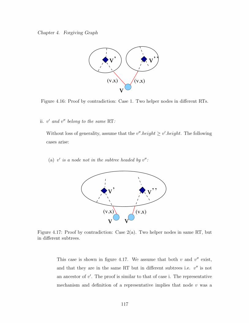
Chapter 4. Forgiving Graph
(v,x)
v’’v’
(v,x)
vFigure 4.16: Proof by contradiction: Case 1. Two helper nodes in different RTs.
ii. v′ and v′′ belong to the same RT:
Without loss of generality, assume that the v′′.height ≥ v′.height. The following
cases arise:
(a) v′ is a node not in the subtree headed by v′′:
v’’v’
(v,x)(v,x)
vvFigure 4.17: Proof by contradiction: Case 2(a). Two helper nodes in same RT, butin different subtrees.
This case is shown in figure 4.17. We assume that both v and v′′ exist,
and that they are in the same RT but in different subtrees i.e. v′′ is not
an ancestor of v′. The proof is similar to that of case i. The representative
mechanism and definition of a representative implies that node v was a
117

Chapter 4. Forgiving Graph
representative in two non-intersecting subtrees in the same RT. This implies
that node v occurs as a leaf twice in that RT. This is not possible.
(b) v′ is a node in the subtree headed by v′′:
v’’
v(v,x)
v’
Figure 4.18: Proof by contradiction: Case 2(b). Two helper nodes in the samesubtree.
This case is shown in figure 4.18. We assume that both v and v′′ exist,
and that they are in the same RT and moreover v′′ is not an ancestor of
v′. Note that by the representative mechanism, when two nodes are to be
joined, the representative of one of them provides the single node that will
be their parent. This new node inherits the other (unused) representative
as its representative. The tree gets built up bottom up with available
representatives propagating upwards. Thus, node v′ will be created before
node v′′. By definition of a representative, neither v′ nor any of its ancestors
can now have v as a representative since v is now already simulating a
helper node. Thus, v′′ was created without any of its children having v as
a representative. However, this is not possible.
Now, we prove part 2. As stated earlier, at each stage of the merge proce-
dure, RTfragments in BTv will merge with their parent. Suppose that v′ is a helper
node simulated by real node v, and v′ is not part of any complete subtree in such a
RTfragment. This means that v′ will be marked red and removed when this stage
118

Chapter 4. Forgiving Graph
of merge is completed (Refer Figure 4.11). Let node y be the root of the com-
plete subtree (i.e. a primary root in that RTfragment) that has v as a leaf node.
Node v′ is an ancestor of node y since v′ cannot be y’s descendant. By definition,
y.Representative = v, since v will be the unique leaf node in y’s subtree not simu-
lating a helper node in that subtree. When the trees are being merged, v may be
asked to create another helper node. Thus, v may have two helper nodes. Also, each
RTfragment has exactly one anchor node. This anchor may be v′ or another node.
Thus, in the repair phase, a real node may simulate at most two helper nodes, and
one of these helper nodes may be an anchor. However, node v′ will be removed as
soon as this stage is completed, and if v′ was an anchor, a new anchor is chosen from
the existing nodes. Since at the end of the merge, BTv collapses to leave one RT,
the extra helper nodes and the edges from the anchor nodes are not present in FGT ,
thus, not contradicting part 1.
Lemma 4.4. After each deletion, the repair phase requires the sending of at most
O(d log n) messages, each of length O(log2n). Moreover, this can be done in parallel
by the neighbors of the deleted node, in time polylog(d, n).
Proof. There are mainly two types of messages exchanged by the algorithm. They
are the probe messages sent by the FindPrRoots() (Algorithm 4.5.5) within a
RT and the messages containing the information about the primary roots exchanged
by the anchors in BTv and among the primary roots themselves (Algorithm 4.5.7:
ComputeHaft()). Let size(BTv) be the number of RTs of BTv. Since a helper
node can split a RT into maximum 3 parts, and there can be at most d helper nodes,
where d is the degree of the deleted node v, size(BTv) ≤ 3d. Now, let us calculate
the number of messages:
• Probe messages (Algorithm 4.5.5): A probe message is generated by an anchor
of a RT. This is similar to the Strip operation (Section 4.4.1). The path that
119

Chapter 4. Forgiving Graph
the probe message follows is the direct path from the originating node to the
rightmost node of the RT. At most 2 messages can be generated for every node
on the way. Each node waits for a reply to its message. If it had a neighbor
as a primary root, it will hear back from it with the root’s identity. If it had
an anchor as a neighbor, it will get an ’end of path’ message. This node will
then reply back to the message it had received from the its neighbor on the
path from the requesting anchor. Thus, each message generated by the request
from the anchor will get a reply back with identities of one or multiple primary
roots or end of path messages. By the property of hafts, each node on this path
will have a primary root as a neighbor, thus, the longest path a message can
take is equal to the diameter of the tree, which is the longest path in the tree.
Let numnodes be the number of nodes and numprobes be number of probe
messages sent in a single RT. The length of the longest path is 2 log numnodes.
Thus,
numprobes ≤ 2.2.2 log numnodes
≤ 8 log n
• Exchange of primary roots lists (Algorithm 4.5.7): At each step of Algo-
rithm 4.5.4 (BottomupRTMerge()), leaves in BTv merge with their par-
ents. Let rtlistmsgs be the number of messages exchanged for every such
merge. The anchors of the leaves of BTv send their primary roots lists to the
parent, which in turn can send both it’s list and the sibling’s list to the child.
Thus, rtlistmsgs = 4. In addition, every anchor will send this list to the pri-
mary roots in its RT, generating at most another log n messages (Let us call
this AtoRmsgs).
As stated earlier, in the BTv, leaves merge with their parents. The number of such
merges before we are left with a single RT is dsize(BTv)/2 − 1e. Also, at most 3
120

Chapter 4. Forgiving Graph
RTs are involved in each merge. Let totmessages be the total number of messages
exchanged. Hence,
totmessages = dsize(BTv)/2− 1e
(3(numprobes+ AtoRmsgs) + rtlistmsgs)
≤ d3d/2− 1e(27 log n+ 4)
∈ O(d log n)
In BTv, leaves and their parents merge. This can be done in parallel such that each
time the level of BTv reduces by one. Within each RT, the time taken for message
passing is still bounded by O(log n) assuming constant time to pass a message along
an edge. Since there are at most dlogde levels, the time taken for passing the mes-
sages is O(log d log n) i.e polylog(d, n). The biggest message exchanged may have
information about the primary roots of upto two RTs. This may be the message
sent by a parent RT in BTv to its children RT. Since there can be at most O(log n)
primary roots, the size of messages containing their ID is O(log2 n).
We now state our main result. Recall that GT is the graph produced after T
steps of our algorithm, while G′T is the graph resulting from the insertions only, with
no deletions or repairs.
Theorem 4.1. The Algorithm ForgivingGraph has the following properties:
1. Degree increase: For any node v in V (GT ), after any number of time steps, T ,
the degree of v in GT is at most 3 times the degree of v in G′T .
2. Stretch: For any nodes x, y in V (GT ), after any number of time steps, T , the
distance between x and y in GT is at most log(n) times the distance in G′T .
121

Chapter 4. Forgiving Graph
3. Cost: After each deletion, the repair phase requires the sending of at most
O(d log n) messages, each of length O(log2n). Moreover, this can be done in
parallel by the neighbors of the deleted node, in time polylog(d, n).
Proof. Part 1 follow directly by construction of our algorithm. Note that for a real
node v in FGT , any degree increase for v is imposed by the edges of its helper node
to hparent(v) and hchildren(v). From lemma 4.3 part 1, we know that, in FGT , node
v can play the role of at most one helper node for any of its neighbors in G′T at any
time (i.e. equal to the degree of v in G′T ). The number of hchildren of a helper node
are never more than 2, because the reconstruction trees are binary trees. Thus the
total degree of v in FGT is at most 3 times its degree in G′T . From observation 4.1
and noting that GT is a homomorphic image of FGT , we can see that the degree of
v in GT is at most 3 times its degree in G′T .
We next show Part 2. We show that the stretch of the Forgiving Graph FGT is
O(D log n), where n is the number of nodes in GT . The distance between any two
nodes x and y cannot increase by more than the factor of the longest path in the
largest RT on the path between x and y. Since the number of nodes in FGT is O(n),
This factor is log n at the maximum. Since there is a homomorphism from the graph
FGT to GT , the result follows directly from observation 4.2.
The proof of Part 3 follows from Lemma 4.4. Note that besides the communica-
tion of the messages discussed, the other operations can be done in constant time in
our algorithm.
122

Chapter 4. Forgiving Graph
4.7.2 Lower Bounds
Theorem 4.2. Let n be a positive integer, α ≥ 3 and β = 12(logα(n− 1)− 1). Then
there exists a graph on n vertices and a vertex deletion such that any way of repairing
this deletion under our model must either increase the degree of some node by more
than a factor of α, or it must increase the distance between some pair of nodes by at
least a factor of β.
Degree(v) = n−1
y
α − 1z
α
y
x
z
Figure 4.19: Deletion of the central node v of a star leads to an increase in thestretch. Here, the healing algorithm can increase the degree of any node by at mosta factor of α.
Proof. Let G be a star on n vertices, where x is the root node, and x has an edge with
each of the other nodes in the graph. The other nodes (besides x) have a degree of
only 1. Let G′ be the graph created after the adversary deletes the node x. Consider
a breadth first search tree, T , rooted at some arbitrary node y in G′. We know that
the self-healing algorithm can increase the degree of each node by at most a factor
of α, thus every node in T besides y can have at most α − 1 children. Let h be the
height of T . Then we know that 1 + α∑h−1
i=0 (α − 1)i ≥ n − 1. This implies that
(α)h+1 ≥ n− 1 for α ≥ 3, or h+ 1 ≥ logα(n− 1). Let z be a leaf node in T of largest
depth. Then, the distance between y and z in G′ is h and the distance between y
and z in G is 2. Thus, β ≥ h/2, and 2β ≥ logα(n− 1)− 1, or β ≥ 12(logα(n− 1)− 1).
This is illustrated in figure 4.19.
123

Chapter 4. Forgiving Graph
Note that the upper bound on the degree increase and stretch of our algorithm is
within a constant factor of matching this lower bound.
4.8 Conclusion
In this chapter, we have presented a distributed data structure that withstands
repeated adversarial node deletions by adding a small number of new edges after
each deletion. Our data structure is efficient and ensures two key properties, even in
the face of both adversarial deletions and adversarial insertions. First, the distance
between any pair of nodes never increases by more than a log n multiplicative factor
than what the distance would be without the adversarial deletions. Second, the
degree of any node never increases by more than a 3 multiplicative factor.
Several open problems remain including the following. Can we design algorithms
for less flexible networks such as sensor networks? For example, what if the only
edges we can add are those that span a small distance in the original network? Can
we extend the concept of self-healing to other objects besides graphs? For example,
can we design algorithms to rewire a circuit so that it maintains its functionality
even when multiple gates fail?
124

Chapter 4. Forgiving Graph
1: given a Graph G(V,E)
Require: each node of G has a unique ID
2: for each node v ∈ G do
3: Init(v)
4: end for
5: while true do
6: if a vertex v is inserted then
7: vertex v and new neighbors add appropriate edges
8: Init(v)
9: else if a vertex v is deleted then
10: DeleteFix(v)
11: end if
12: end while
Algorithm 4.5.1: Forgiving graph: The main function.
1: for each edge(v, x) do
2: (v, x).Representative = v
3: set other fields to NULL
4: end for
Algorithm 4.5.2: Init(v): initialization of the node v
125

Chapter 4. Forgiving Graph
1: Nset =
2: for each edge(v, x) do
3: if (v, x).hashelper = TRUE then
4: Nset = Nset ∪ (v, x).hparent ∪ (v, x).hrightchild
5: end if
6: Nset = Nset ∪ (v, x).endpoint
7: end for
8: Nodes in Nset make new edges to make a balanced binary tree BTv(Nset, Ev)
9: BottomupRTMerge(BTv, v)
10: delete the edges Ev
Algorithm 4.5.3: DeleteFix(v): Self-healing on deletion of a node
126

Chapter 4. Forgiving Graph
1: if BTv has only one node then
2: return
3: end if
4: for y ∈ BTv do
5: if y is a real node then
6: let y.PrRoots← y
7: else if y = (v, x).endpoint then
8: y.PrRoots← FindPrRoots(y, 1, (v, x),TRUE, y )
9: else if y.helper.hparent = v OR y.helper.hleftchild = v OR
y.helper.hrightchild = v then
10: let y.PrRoots← FindPrRoots(y, v.desccount, v.helper,TRUE, y)
11: else
12: let y.PrRoots← FindPrRoots(y, v.desccount, v.helper,FALSE, y)
13: end if
14: end for
15: for all nodes y s.t. node y is a parent of a leaf in BTv do
16: if y has two children in BTv then
17: Haft Merge(y, y ’s left child in BTv, y ’s right child in BTv)
18: else
19: Haft Merge(y, y’s left child, NULL)
20: end if
21: end for
22: BottomupRTMerge(BTv) // New leaf nodes merge again till only one is left.
Algorithm 4.5.4: BottomupRTMerge(BTv, v): The nodes of BTv merge their
RTs starting from the leaves going up forming a new BTv.
127

Chapter 4. Forgiving Graph
1: if y is an Anchor node AND y 6= origin then
2: return NULL // Anchors reject probe messages from other anchors.
3: end if
4: if Breakflag = TRUE AND (sender = y.hrightchild OR sender = y.hleftchild )
then
5: y.desccount = y.desccount - numchild
6: end if
7: if y.desccount = 2y.height then
8: if TestPrimaryRoot(y) = TRUE then
9: return y,FindPrRoots(y.hparent, 0, y, Breakflag, origin)
10: else
11: return FindPrRoots(y.hparent, 0, y, Breakflag, origin) // Node itself
not a primary root but parent maybe.
12: end if
13: else
14: mark node red
15: if exists(y.hleftchild) AND sender 6= y.hleftchild then
16: FindPrRoots(y.hleftchild, y.desccount, y, Breakflag, origin)
17: else if exists(y.hrightchild) AND sender 6= y.hrightchild then
18: FindPrRoots(y.hrightchild, y.desccount, y, Breakflag, origin)
19: else if exists(y.hparent) AND sender 6= y.hparent then
20: FindPrRoots(y.hparent, y.desccount, y, Breakflag, origin)
21: end if
22: end if
Algorithm 4.5.5: FindPrRoots(y, numchild, sender, Breakflag, origin): Find
primary roots in the RTfragment (Section 4.5 of main text) containing node y. If
Breakflag is set, the tree is a RTfragment formed due to the deletion of the node
prior to any merges and the nodes need to adjust their descendant count.
128

Chapter 4. Forgiving Graph
1: if y.desccount = 2y.height then
2: if y.hparent = NULL then
3: return TRUE
4: else if y.hparent.desccount 6= 2y.hparent.height then
5: return TRUE
6: end if
7: end if
8: return FALSE
Algorithm 4.5.6: TestPrimaryRoot(y): Tell if helper node y is a primary root
in RT
1: Nodes p, ` and r exchange p.PrRoots, `.PrRoots(l), PrRoots(r)
2: let RT← MakeRT(PrRoots(p), `.PrRoots, r.PrRoots)
3: if p is marked red then
4: p transfers its edges in BTv to one of p.PrRoots // p needs to be removed, BTv
needs to be maintained
5: end if
6: remove all helper nodes marked red // Some helper nodes marked red may have
been reused and unmarked by MakeRT
Algorithm 4.5.7: Haft Merge(p, `, r): Merge the hafts mediated by anchors p, `
and r
1: for all y ∈ (PRoots1 ∪ PRoots2 ∪ PRoots3) do
2: let T ← ComputeHaft(PRoots1, PRoots2, PRoots3)
3: make helper nodes and set fields and make edges according to T
4: end for
Algorithm 4.5.8: MakeRT(PRoots1, PRoots2, PRoots3): The sets of Primary
roots make a new RT
129

Chapter 4. Forgiving Graph
1: let R = PRoots1 ∪ PRoots2 ∪ PRoots3
2: let L = R sorted in ascending order of number of children, NodeID
3: suppose L is (r1, r2, . . . , rk) where the ri are the k ordered primary roots.
4: set ctr = 1, count = k
5: while ctr < count do
6: if rctr.numchildren = rctr+1.numchildren then
7: Make helper node helper(rctr.Representative). Initialize fields to NULL.
8: make helper(rctr.Representative) the parent of rctr and rctr+1
9: if rctr is a real node then
10: set helper(rctr.Representative).height = 1
11: else
12: set helper(rctr.Representative).height = 2rctr.height
13: end if
14: set helper(rctr.Representative).Representative = rctr+1.Representative
15: remove rctr, rctr+1, insert helper(rctr.Representative) in correct place in L.
16: set ctr ← ctr − 1, count← count− 1
17: end if
18: set ctr ← ctr + 1,
19: end while
20: set ctr = 1
21: while ctr < count do
22: make helper node helper(rctr+1.Representative). Initialise its fields to NULL
23: set helper(rctr+1.Representative).hleftchild = rctr+1
24: set helper(rctr+1.Representative).hrightchild = rctr
25: set helper(rctr+1.Representative).height = rctr+1.height + 1
26: set helper(rctr+1.Representative).Representative = rctr.Representative
27: In L, replace rctr+1 by helper(rctr+1.Representative)
28: end while
Algorithm 4.5.9: ComputeHaft(PRoots1,PRoots2,PRoots3): (Implementation
of Haft Merge) The primary roots compute the new haft
130

Chapter 5
Future Directions
There is no such thing as a failed
experiment, only experiments with
unexpected outcomes
Richard Buckminster Fuller
In this chapter, we point out some related open problems and discuss the future
directions in which this research can be extended.
5.1 Empirical study of self-healing algorithms be-
yond assumptions
How would our algorithms perform beyond the assumptions of the model we have
used? There are certain assumptions our algorithms make and we would like to
know how well our algorithms perform even when those assumptions don’t hold e.g.
our model assumes single failure before each recovery. How would our algorithms
perform if there are multiple failures in close physical or temporal proximity? Akin
to an ecological disaster, we would see how the algorithms perform if a set of nodes
131

Chapter 5. Future Directions
(a clump of species) are simultaneously deleted or there are cascading failures. We
will also place restrictions on the topology of the network and add additional rules
to the algorithm to simulate different networks found in nature. In particular, we
have already begun work on simulating ForgivingGraph for these purposes.
5.2 Routing in Self-healing structures
Can we implement efficient updates to routing tables? Small changes to the network,
e.g., deletion of an edge or a node can lead to major changes in the tables. Can
our algorithms keep track of these? Self-healing routing is an important research
question especially given the dynamic nature of modern networks [30, 21, 45]. We
will like to propose solutions in our framework which incorporate routing in addition
to the invariants we already maintain. This could involve proposing efficient routing
schemes to go with our self-healing structures or developing new structures that help
routing.
5.3 Load balanced Self-healing
Trees are not the best structure for effective load balancing e.g. in a balanced tree,
half of the paths will go through the root. Can we improve the load balancing using a
different self-healing data structure? Good load balancing would be ensured if upon
healing there are not likely to be bottlenecks for communication traffic. There has
been some previous work on load balancing in structured P2P systems [32]. This
may also be related to the earlier question (Section 5.2) on self-healing Routing.
There are many interesting ideas we are looking at out there which may potentially
contribute to a solution that we are looking at e.g. The Chord P2P structure [54],
Skip graphs [54], and Small-world network models [36].
132

Chapter 5. Future Directions
5.4 Self-healing in Sensor Networks
Directional antennas are increasingly becoming important in sensor networks e.g.
[26]. They also allow us to use our concept of self-healing where we have an edge in
the underlying graph for two nodes in communication with each other. In a wireless
ad-hoc network multi-hop connectivity can be easily lost when a transceiver goes
silent and does not relay messages any longer. Successful pairwise communication
occurs in a wireless network only in the absence of interference which is usually
achieved by frequency or time or code division multiplexing, i.e., by assigning non-
interfering channels (colors) to the pairwise links (edges) that are necessary for global
connectivity. Therefore, to restore connectivity after a node failure, it is important
to also restore an interference-free channel assignment for the pairwise links in the
repaired network.
In the disk graph model of a wireless ad-hoc network, there are n transceivers and
the transmission and reception range of a transceiver u is a disk D(u) centered at u
with radius r(u). The transceivers are vertices of a directed graph G = (V,E). The
directed edge u→ v belongs to E if and only if v is in D(u). Two transceivers u and
v can communicate directly (without intermediate hops) if and only if both directed
edges u → v and v → u are present. We say that a pair of transceivers (u, v) are
connected if there exists a path between u and v consisting of bidirectional edges.
Two edges (u, v) and (p, q) may exhibit primary interference if either u ∈ p, q
or v ∈ p, q, i.e., if they have a common vertex. They may exhibit secondary
interference if they share a common edge i.e. there is an edge whose one end-point
is either u or v and the other is either p or q.
The question of maintaining this interference-free communication graph can then
be reduced to maintenance of strong edge coloring where each edge is assigned a color
such that no interfering edge shares a color, in the presence of an adversary. We can
133

Chapter 5. Future Directions
again assume that the adversary removes one node at a time and the neighbors
are alerted of this. One possible approach is to use the self-healing idea such as the
notion of ”wills” (as in Forgiving Tree) to compute an efficient, local way to repair the
network by re-connecting (a subset of) the nodes in the neighborhood of the deleted
vertex. We can then use a distributed, randomized algorithm (i.e., a protocol), a
la Luby [41], to implement the repair. In [6] Barett at al adapted Luby’s algorithm
to the case of distance-2 coloring and showed that it was sufficient for each node to
know the so-called “active degree” to determine its wake-up probability. Much of
the ideas in this section were from discussion with Shripad Thite (Google).
5.5 Self-healing/ Behavioral robustness in Social
Networks
There are some interesting avenues to explore in the context of robustness in social
networks. Some of the questions in this context may involve achieving behavioral
robustness as opposed to topological invariance like we have used so far in our self-
healing work. One of the question we want to explore is the following: Does a
phenomena like the minority game which normally achieves equilibrium achieves
homeostasis even in the presence of an adversary. This has the flavor of behavioral
invariance. In [33], Willemien et al show that a learning process in which players
best-reply to a history of limited length and in which they have a preference for more
recent best replies (”recency bias”) eventually settles down in one of the pure Nash
equilibria (optimal anti-coordination) if the memory length of players is at least 2.
The proof uses the fact that you can construct a path from any initial history to a
state where players play according to a pure Nash equilibrium in each following time
period, and that such a path will occur with probability 1 in the long run. This gives
134

Chapter 5. Future Directions
an algorithm for reaching an anti-coordination equilibrium if players best-reply to
beliefs based on a limited history of play and they have a recency bias.
Our idea is to study what will happen to the equilibrium if an adversary (in the
sense of external perturbations) is introduced into the mix. Will we still achieve the
anti-coordination equilibrium?, and what are the implications?
5.6 Self-* problems
Can we go beyond Self-healing (demand even stronger guarantees)? There is strong
interest in the so-called self-* algorithms. We have earlier discussed these properties
in Section 1.5.1. One such objective is self-stabilization. A distributed system that is
self-stabilizing will end up in a correct state no matter what state it is initialized with.
This is a highly desirable property for distributed systems, and worth investigating.
Another direction would be too look at the network layers themselves. Our work is
based on overlay networks. However, it may be beneficial to consider what happens
below that layer, at the physical layer itself, to come up with practical, efficient and
robust network designs.
5.7 Evolution of social and computer networks
and study of group formation
It is important to study the mechanisms behind the formation and evolution of
networks, particularly, networks like the Internet, and social networks, in particular
with regards to their stability and self-* properties. Techniques from various areas
like game theory can often be profitably applied here. There are many models seeking
to explain network formation e.g. [40]; Some models seek to explain the formation of
135

Chapter 5. Future Directions
networks in a game theoretic manner by having nodes as players making connections
(edges) with other players to maximize their utility function [16].
There is interest in discovering mechanisms for formation of groups. Our at-
tempts at simple toy models suggest this is a difficult problem. However, there has
been interesting research in this area incorporating both theoretical and experimental
(including field observations) work. Dan Rubenstein, an ecologist from Princeton,
collected data on the social structure graphs of the thriving plains zebra and the en-
dangered Grevy’s zebras, from the plains of Africa. He and Tanya Berger-Wolff, from
University of Illinois Chicago, then modeled the Zebra’s group behavior by looking at
the network of their social behavior to find interesting patterns [52, 56]. Jared Saia
and Tanya Berger-Wolff have also proposed mathematical and computational frame-
work that enables analysis of dynamic social networks and that explicitly makes use
of information about when social interactions occur [7]. There are also many inter-
esting data sets e.g. on mobile phone usage patterns [39], which can help investigate
such questions as routing of messages, group formation and social motivation.
There are many interesting questions: How do groups self-heal i.e are groups
sensitive to perturbation, leaving and joinings of agents? What are the mechanisms
that explain formation and dissolution of groups in real networks? Can we propose
such game theoretic cost functions? When agents cooperate to form a group, how
does that influence formation of other groups?
5.8 Byzantine agreement: Distributed computing
in presence of byzantine faults
This section owes itself to discussions with Professor Valerie King. The failure models
we have considered so far ignore byzantine faults (e.g. by adversarial code corrup-
136

Chapter 5. Future Directions
tion), but it is important for the network to be able to function/self-heal in presence
of these faults. A fundamental problem in distributed computing is that of coordi-
nating behavior by processors in the presence of an adversary who controls a constant
fraction of processors. At its most basic, it is formulated as the Byzantine Agreement
Problem. Each of n processors are given an input bit; they execute a protocol, at
the end of which all output the same bit equal to one of their input bits.
This problem, in the asynchronous model (an adversary controls the order in
which messages are delivered), is known to be impossible to solve deterministically
in the full information model, i.e., if the adversary has access to all messages sent
and there are no cryptographic assumptions made. A randomized protocol exists in
which each processor has private random bits but it requires an exponential number of
messages. Both of these results were shown in the 1980’s. Last year, Kapron, Kempe,
King, Saia and Sanwalani [31] showed a polylogarithmic time protocol which succeeds
with high probability for this problem if the choice of corrupt processors is made
independently of the random bits, and the adversary is “non-adaptive”. In addition,
King and Saia showed that O(n3/2) total bits of communication suffice [34]. Without
the assumption, all known Byzantine Agreement protocols in the synchronous model
(where messages are delivered in rounds) and the asynchronous model use Ω(n2)
messages, even with private channels and cryptographic assumptions.
Several intriguing problems remain open, in decreasing order of difficulty:
1. Can we close the gap between the lower bound of n2 and the upper bound
of exponential time for asynchronous Byzantine agreement (with an adaptive
adversary) in the full information model?
2. Can we do Byzantine agreement with cryptography or private channels with
an adaptive adversary in o(n2) bits per processor? Is it possible to prove a
nontrivial lower bound here? Is there a practical protocol for this? (Recently,
137

Chapter 5. Future Directions
King and Saia have published an algorithm which solves this problem in the
synchronous model [35]. Their algorithm assumes private channels and takes
only O(√n) bits per processor and has polylog latency).
3. Can we load balance the Byzantine agreement problem so that no processor
uses more than o(n) bits with the assumption, for the synchronous model? For
the asynchronous model?
4. Can we enhance the protocols designed by King and Saia, so that they are
robust to an adversary who can also remove and insert new nodes, some of
which are corrupt, still in the full information model?
Techniques for proving lower bounds for randomized distributed problems like
this are scarce and may involve techniques from communication complexity. There
is a well known method for deterministic lower bounds in distributed computing
using algebraic topology, but there is no known extension to randomized algorithms.
This would be interesting to explore. Any answer to the first question will be a major
breakthrough in a widely studied problem area that has been open for over 25 years.
138

References
[1] David Andersen, Hari Balakrishnan, Frans Kaashoek, and Robert Morris. Re-silient overlay networks. SIGOPS Oper. Syst. Rev., 35(5):131–145, 2001.
[2] Villu Arak. What happened on August 16, August 2007.http://heartbeat.skype.com/2007/08/what-happened-on-august-16.html.
[3] Baruch Awerbuch, Boaz Patt-Shamir, David Peleg, and Michael Saks. Adaptingto asynchronous dynamic networks (extended abstract). In STOC ’92: Pro-ceedings of the twenty-fourth annual ACM symposium on Theory of computing,pages 557–570, New York, NY, USA, 1992. ACM.
[4] Albert-Laszlo Barabasi and Reka Albert. Emergence of scaling in random net-works. Science, 286:509, 1999.
[5] Albert-Laszlo Barabasi and Eric Bonabeau. Scale-free networks. ScientificAmerican, pages 50–59, 2003.
[6] Christopher L. Barrett, V. S. Anil Kumar, Madhav V. Marathe, Shripad Thite,and Gabriel Istrate. Strong edge coloring for channel assignment in wireless radionetworks. In PERCOMW ’06: Proceedings of the 4th annual IEEE internationalconference on Pervasive Computing and Communications Workshops, page 106,Washington, DC, USA, 2006. IEEE Computer Society.
[7] Tanya Y. Berger-Wolf and Jared Saia. A framework for analysis of dynamicsocial networks. In KDD ’06: Proceedings of the 12th ACM SIGKDD interna-tional conference on Knowledge discovery and data mining, pages 523–528, NewYork, NY, USA, 2006. ACM.
[8] Andrew Berns and Sukumar Ghosh. Dissecting self-* properties. Self-Adaptiveand Self-Organizing Systems, International Conference on, 0:10–19, 2009.
139

References
[9] I-Ching C. Boman. Algorithms for self-healing networks. M.S. Thesis, ComputerScience, University of New Mexico., 2006.
[10] Iching Boman, Jared Saia, Chaouki T. Abdallah, and Edl Schamiloglu. Brief an-nouncement: Self-healing algorithms for reconfigurable networks. In Symposiumon Stabilization, Safety, and Security of Distributed Systems(SSS), 2006.
[11] Edith Cohen. Size-estimation framework with applications to transitive clo-sure and reachability. In Proceedings of the Foundations of Computer Science(FOCS), 1994.
[12] Edsger W. Dijkstra. Self-stabilizing systems in spite of distributed control.Commun. ACM, 17(11):643–644, November 1974.
[13] Shlomi Dolev. Self-stabilization. MIT Press, Cambridge, MA, USA, 2000.
[14] Shlomi Dolev and Nir Tzachar. Empire of colonies: Self-stabilizing and self-organizing distributed algorithm. Theor. Comput. Sci., 410(6-7):514–532, 2009.
[15] Robert D. Doverspike and Brian Wilson. Comparison of capacity efficiency ofdcs network restoration routing techniques. J. Network Syst. Manage., 2(2),1994.
[16] Alex Fabrikant, Ankur Luthra, Elitza Maneva, Christos H. Papadimitriou, andScott Shenker. On a network creation game. In PODC ’03: Proceedings of thetwenty-second annual symposium on Principles of distributed computing, pages347–351, New York, NY, USA, 2003. ACM.
[17] Ken Fisher. Skype talks of ”perfect storm” that caused outage, clarifies blame,August 2007. http://arstechnica.com/news.ars/post/20070821-skype-talks-of-perfect-storm.html.
[18] T. Frisanco. Optimal spare capacity design for various protection switchingmethods in ATM networks. In Communications, 1997. ICC 97 Montreal, ’To-wards the Knowledge Millennium’. 1997 IEEE International Conference on, vol-ume 1, pages 293–298, 1997.
[19] Ned Glick. Breaking records and breaking boards. The American MathematicalMonthly, 85(1):2–26, January 1978.
[20] Sanjay Goel, Salvatore Belardo, and Laura Iwan. A resilient network that canoperate under duress: To support communication between government agenciesduring crisis situations. Proceedings of the 37th Hawaii International Conferenceon System Sciences, 0-7695-2056-1/04:1–11, 2004.
140

References
[21] Chao Gui and Prasant Mohapatra. Short: self-healing and optimizing routingtechniques for mobile ad hoc networks. In In Proceedings of MobiHoc, pages279–290. ACM Press, 2003.
[22] Yukio Hayashi and Toshiyuki Miyazaki. Emergent rewirings for cascades oncorrelated networks. cond-mat/0503615, 2005.
[23] Thomas P. Hayes, Jared Saia, and Amitabh Trehan. The forgiving graph: adistributed data structure for low stretch under adversarial attack. In PODC ’09:Proceedings of the 28th ACM symposium on Principles of distributed computing,pages 121–130, New York, NY, USA, 2009. ACM.
[24] Tom Hayes, Navin Rustagi, Jared Saia, and Amitabh Trehan. The forgivingtree: a self-healing distributed data structure. In PODC ’08: Proceedings of thetwenty-seventh ACM symposium on Principles of distributed computing, pages203–212, New York, NY, USA, 2008. ACM.
[25] Petter Holme and Beom Jun Kim. Vertex overload breakdown in evolving net-works. Physical Review E, 65:066109, 2002.
[26] Zhuochuan Huang, Chien chung Shen, Chavalit Srisathapornphat, and ChaipornJaikaeo. Topology control for ad hoc networks with directional antennas. InProc. IEEE Int. Conference on Computer Communications and Networks, pages16–21, 2002.
[27] IBM. http://www.research.ibm.com/autonomic/manifesto/autonomic comput-ing.pdf.
[28] IBM. http://www.research.ibm.com/autonomic/research/papers/AC VisionComputer Jan 2003.pdf.
[29] Rainer R. Iraschko, M. H. MacGregor, and Wayne D. Grover. Optimal capac-ity placement for path restoration in STM or ATM mesh-survivable networks.IEEE/ACM Trans. Netw., 6(3):325–336, 1998.
[30] M. Lisee J.W. Branch and B.K. Szymanski. Shr: self-healing routing for wirelessad hoc sensor networks. Proc. Int. Symposium on Performance Evaluation ofComputer and Telecommunication Systems SPECTS’07, pages 5–14, 2007.
[31] Bruce Kapron, David Kempe, Valerie King, Jared Saia, and Vishal Sanwalani.Fast asynchronous byzantine agreement and leader election with full informa-tion. In SODA ’08: Proceedings of the nineteenth annual ACM-SIAM sympo-sium on Discrete algorithms, pages 1038–1047, Philadelphia, PA, USA, 2008.Society for Industrial and Applied Mathematics.
141

References
[32] Ananth Rao Karthik, Ananth Rao, Karthik Lakshminarayanan, Sonesh Surana,Richard Karp, and Ion Stoica. Load balancing in structured p2p systems. In2nd International Workshop on Peer-To-Peer Systems (IPTPS), 2003.
[33] W. Kets and M. Voorneveld. Congestion, equilibrium and learning: The minor-ity game. Discussion Paper 2007-61, Tilburg University, Center for EconomicResearch, 2007.
[34] Valerie King and Jared Saia. From almost everywhere to everywhere: Byzantine
agreement with o(n3/2) bits. In DISC, pages 464–478, 2009.
[35] Valerie King and Jared Saia. Breaking the o(n2) bit barrier: Scalable byzantineagreement with an adaptive adversary, 2010. http://arxiv.org/abs/1002.4561.
[36] Jon Kleinberg. The small-world phenomenon: an algorithm perspective. InSTOC ’00: Proceedings of the thirty-second annual ACM symposium on Theoryof computing, pages 163–170, New York, NY, USA, 2000. ACM.
[37] Fabian Kuhn, Stefan Schmid, Joest Smit, and Roger Wattenhofer. A Blueprintfor Constructing Peer-to-Peer Systems Robust to Dynamic Worst-Case Joinsand Leaves. In 14th IEEE International Workshop on Quality of Service(IWQoS), Yale University, New Haven, Connectitut, USA, June 2006.
[38] Fabian Kuhn, Stefan Schmid, and Roger Wattenhofer. A Self-Repairing Peer-to-Peer System Resilient to Dynamic Adversarial Churn. In 4th InternationalWorkshop on Peer-To-Peer Systems (IPTPS), Cornell University, Ithaca, NewYork, USA, Springer LNCS 3640, February 2005.
[39] MIT Media Lab. The reality mining dataset.http://reality.media.mit.edu/dataset.php.
[40] Silvio Lattanzi and D. Sivakumar. Affiliation networks. In STOC ’09: Pro-ceedings of the 41st annual ACM symposium on Theory of computing, pages427–434, New York, NY, USA, 2009. ACM.
[41] M Luby. A simple parallel algorithm for the maximal independent set problem.In STOC ’85: Proceedings of the seventeenth annual ACM symposium on Theoryof computing, pages 1–10, New York, NY, USA, 1985. ACM.
[42] Om Malik. Does Skype Outage Expose P2Ps Limitations?, August 2007.http://gigaom.com/2007/08/16/skype-outage.
[43] Gurmeet Singh Manku, Moni Naor, and Udi Wieder. Know thy neighbor’sneighbor: the power of lookahead in randomized p2p networks. In Proceedingsof the 36th ACM Symposium on Theory of Computing (STOC), 2004.
142

References
[44] Muriel Medard, Steven G. Finn, and Richard A. Barry. Redundant trees forpreplanned recovery in arbitrary vertex-redundant or edge-redundant graphs.IEEE/ACM Transactions on Networking, 7(5):641–652, 1999.
[45] Thomas Meyer, Lidia Yamamoto, and Christian Tschudin. A self-healing multi-path routing protocol. In BIONETICS ’08: Proceedings of the 3rd InternationalConference on Bio-Inspired Models of Network, Information and ComputingSytems, pages 1–8, ICST, Brussels, Belgium, Belgium, 2008. ICST (Institutefor Computer Sciences, Social-Informatics and Telecommunications Engineer-ing).
[46] Matt Moore. Skype’s outage not a hang-up for user base, Au-gust 2007. http://www.usatoday.com/tech/wireless/phones/2007-08-24-skype-outage-effects-N.htm.
[47] Adilson E Motter. Cascade control and defense in complex networks. PhysicalReview Letters, 93:098701, 2004.
[48] Adilson E Motter and Ying-Cheng Lai. Cascade-based attacks on complexnetworks. Physical Review E, 66:065102, 2002.
[49] Kazutaka Murakami and Hyong S. Kim. Comparative study on restorationschemes of survivable ATM networks. In INFOCOM (1), pages 345–352, 1997.
[50] Moni Naor and Udi Wieder. Know thy neighbor’s neighbor: Better routing forskip-graphs and small worlds. In in Proc. of IPTPS, 2004, pages 269–277, 2004.
[51] Bill Ray. Skype hangs up on users, August 2007.http://www.theregister.co.uk/2007/08/16/skype down/.
[52] Julie Rehmeyer. Social networking for zebras.http://www.sciencenews.org/view/generic/id/9150/title/Math Trek SocialNetworking for Zebras.
[53] Jared Saia and Amitabh Trehan. Picking up the pieces: Self-healing in recon-figurable networks. In IPDPS. 22nd IEEE International Symposium on Paralleland Distributed Processing., pages 1–12. IEEE, April 2008.
[54] Ion Stoica, Robert Morris, David Liben-Nowell, David R. Karger, M. FransKaashoek, Frank Dabek, and Hari Balakrishnan. Chord: a scalable peer-to-peerlookup protocol for internet applications. IEEE/ACM Trans. Netw., 11(1):17–32, 2003.
143

References
[55] Brad Stone. Skype: Microsoft Update Took Us Down, August2007. http://bits.blogs.nytimes.com/2007/08/20/skype-microsoft-update-took-us-down.
[56] Chayant Tantipathananandh, Tanya Berger-Wolf, and David Kempe. A frame-work for community identification in dynamic social networks. In KDD ’07:Proceedings of the 13th ACM SIGKDD international conference on Knowledgediscovery and data mining, pages 717–726, New York, NY, USA, 2007. ACM.
[57] Gerard Tel. Introduction to distributed algorithms. Cambridge University Press,New York, NY, USA, 1994.
[58] B. van Caenegem, N. Wauters, and P. Demeester. Spare capacity assignmentfor different restoration strategies in mesh survivable networks. In Communica-tions, 1997. ICC 97 Montreal, ’Towards the Knowledge Millennium’. 1997 IEEEInternational Conference on, volume 1, pages 288–292, 1997.
[59] Jean G. Vaucher. Building optimal binary search trees from sorted values inO(n) time. In Essays in Memory of Ole-Johan Dahl, pages 376–388, 2004.
[60] Whatis.com. http://searchcio-midmarket.techtarget.com/sDefinition/0,,sid183gci906565,00.html.
[61] Yijun Xiong and Lorne G. Mason. Restoration strategies and spare capacityrequirements in self-healing ATM networks. IEEE/ACM Trans. Netw., 7(1):98–110, 1999.
144