Embed Size (px)
Citation preview

Journal of International Economics 48 (1999) 7–35
Networks versus markets in international trade
*James E. RauchDepartment of Economics, University of California, La Jolla, San Diego, CA 92093-0508, USA
Received 27 June 1996; received in revised form 26 August 1997; accepted 29 October 1997
Abstract
I propose a network/search view of international trade in differentiated products. Ipresent evidence that supports the view that proximity and common language/colonial tiesare more important for differentiated products than for products traded on organizedexchanges in matching international buyers and sellers, and that search barriers to trade arehigher for differentiated than for homogeneous products. I also discuss alternativeexplanations for the findings. 1999 Elsevier Science B.V. All rights reserved.
Keywords: Trade; Networks; Markets
JEL classification: F10
1. Introduction
It is well known that very few manufactured (as opposed to primary)commodities are traded on organized exchanges. It is also well understood that theheterogeneity of manufactures along the dimensions of both characteristics andquality interferes with the ability of their prices to signal relative scarcity. I arguethat this uninformativeness of prices prevents ‘globally scanning’ traders fromsubstituting for organized exchanges in matching international buyers and sellersof differentiated products. Instead connections between sellers and buyers aremade through a search process that because of its costliness does not proceed until
*Corresponding author. Tel.: 001-619-534-2405; fax: 001-619-534-7040.E-mail address: [email protected] (J.E. Rauch)
0022-1996/99/$ – see front matter 1999 Elsevier Science B.V. All rights reserved.PI I : S0022-1996( 98 )00009-9
8 J.E. Rauch / Journal of International Economics 48 (1999) 7 –35
the best match is achieved. This search is strongly conditioned by proximity andpreexisting ‘ties’ and results in trading networks rather than ‘markets’.
This paper will explore the consequences of this network /search view at amacro level by examining world trade flows. In a companion paper (Rauch, 1996)I explore the consequences of this view at a micro level by examining tradebehavior, institutions, and policies in a partial equilibrium context. Section 2 ofthis paper expands the argument adumbrated in the previous paragraph sufficientlyto allow for empirical application. Section 3 uses a gravity model of internationaltrade to see if proximity and common language/colonial ties are more importantfor differentiated products than for products traded on organized exchanges inmatching international buyers and sellers. Section 4 examines whether differen-tiated products tend to be less traded than homogeneous products, indicating thatsearch costs are acting as barriers to trade. Section 5 considers alternativeexplanations, not based on the network /search view, for the findings in thepreceding two sections. Conclusions and suggestions for further research arepresented in Section 6.
2. Organized exchanges, reference prices, or neither
In the empirical work below I will divide internationally traded commoditiesinto three groups: those traded on organized exchanges, those not traded onorganized exchanges but nevertheless possessing what I shall call ‘referenceprices’, and all other commodities. In this section I will give the theoreticalmotivation for this tripartite division.
Let us first consider why some commodities are traded on organized exchangesand others are not. The conventional wisdom is that there is a cost to setting up‘markets’ (organized exchanges) that is independent of the volume of transactions,and that this nonconvexity will not allow a market to open if the expected volume
1of transactions at the price expected to prevail in equilibrium is too small. For thesake of concreteness, let us attempt to apply this conventional wisdom to twocommodities at the three-digit level of the Standard International Trade Classifica-tion (SITC), which is the least disaggregated level for which I will attempt tocategorize commodities in the empirical work below. The two commodities areFootwear (SITC 851) and Lead (SITC 685, not to be confused with Lead Ores andConcentrates, SITC 2874). Suppose we use the dollar values of international tradein 1990 between the 63 countries in my sample below to indicate the ‘thickness’ of
1Much to my surprise, I could not find a formalization of this ‘conventional wisdom’ in the literature.The closest I found is Heller (1993). Market formation involves set-up costs in his model, but his focusis on coordination failure where it is mutually profitable to open markets in complementarycommodities but not to open one of them individually.

J.E. Rauch / Journal of International Economics 48 (1999) 7 –35 9
the markets in these commodities, admitting that this is a bad proxy because itexcludes domestic trade and does not account for the average size of transactions.The figures are $27.3 billion for Footwear and $1.3 billion for Lead, of whichnearly 90 percent is Lead and Lead Alloys, Unwrought (SITC 6851) as opposed toLead and Lead Alloys, Worked (SITC 6852). Unwrought lead is traded on theLondon Metal Exchange while footwear is not listed on any organized exchange.This information appears to contradict the conventional wisdom on formation oforganized exchanges. However, one could argue that ‘footwear’ is not a well-defined commodity and needs to be disaggregated into various types of shoes, eachone of which may have a volume of transactions smaller than that of lead. As weknow, in the limit this process of disaggregation leads to shoes for which there isonly one supplier: shoes are ‘branded’ or differentiated products.
Without necessarily endorsing this argument, let us explore it further bycontrasting Footwear with Polymerization and Copolymerization Products (SITC583). 1990 international trade in these chemicals for the 63 countries in my sampleamounted to $47.6 billion. Like Footwear, they are not listed on any organizedexchange, perhaps because they can be disaggregated into types for each of whichthe market is too ‘thin’. Does this mean that Polymerization and CopolymerizationProducts should be treated in the same way as Footwear in the empirical analysisbelow?
The answer is no. Polymerization and Copolymerization Products are not‘branded’: prices can be quoted for these products without mentioning the name ofthe manufacturer, and these ‘reference prices’ are found to be sufficiently useful byindustry actors to be worth listing in trade publications. For example, a price perpound of Polyoxyethylene Sorbitan Monostearate is quoted weekly in ChemicalMarketing Reporter on the basis of surveys of suppliers. Abstracting fromtransportation costs, it is then possible for traders to assess the profitability ofshipping polymerization and copolymerization products between any two countriessolely on the basis of the prices prevailing at the ports of those two countries. Oneor more traders specialized in a given one of these chemicals can keep informed ofits prices around the globe and perform international commodity arbitrage,matching distant buyers and sellers just as would traders on an organizedexchange. As far as empirical analysis of matching international buyers and sellersis concerned, then, the reason to treat commodities traded on organized exchangesdifferently from commodities that only have reference prices is that we know theformer have specialized traders that centralize price information while the same isonly potentially true for the latter.
Shoes, on the other hand, do not have reference prices. Any observed price atanother location must be adjusted for multidimensional differences in characteris-tics, and the adjustment depends on the varieties of shoes available at that locationand the distribution of consumer preferences over varieties at that location. I claimthat these informational demands are too great to permit international commodity
10 J.E. Rauch / Journal of International Economics 48 (1999) 7 –35
2arbitrage, and therefore traders will instead engage in a sequential search forbuyers / sellers that terminates when some ‘reservation match’ is achieved. Thissearch is facilitated by proximity and common language, and by any contacts who‘know the market’. Of course the trader’s network of contacts will also be stronglyinfluenced by proximity and common language, and by preexisting ties such asthose between former colonies and the colonial power. Discussing ‘psychologicalbarriers’ to trade, Nothdurft (1992), pp. 39–40) states, ‘Typically, trade beginsclose to home and then, as experience and confidence grows, expands ‘like rings in
3the water,’ as one official of the Stockholm Chamber of Commerce put it.’For the purposes of the empirical work below, we can summarize the discussion
of this section as follows. Possession of a reference price distinguishes homoge-neous from differentiated products. Homogeneous commodities can be furtherdivided into those whose reference prices are quoted on organized exchanges andthose whose reference prices are quoted only in trade publications. The network /search model should apply most strongly to differentiated products and mostweakly to products traded on organized exchanges, with its applicability to otherhomogeneous products unclear. Thus proximity and common language/colonialties should have the greatest effects on matching international buyers and sellers ofdifferentiated products, and search costs should act as the greatest barrier to tradefor differentiated products. These hypotheses will be examined in Section 3Section 4, respectively.
3. Evidence from a gravity model of trade
3.1. The gravity model
The standard (indeed, the only) empirical framework used to predict howcountries match up in international trade is the gravity model. This model takes itsname from the prediction that the volume of trade between two countries will bedirectly proportional to the product of their economic masses (as measured byGDP or GNP) and inversely proportional to the distance between them. AsHarrigan (1994) and others have pointed out, at least two different theoretical
2Here I find it helpful to have in mind Hahn (1971) definition of markets as activities that transform‘named’ goods into ‘anonymous’ goods. One could argue that the ‘anonymity’ provided by the pricesystem is what makes international commodity arbitrage possible. It is not possible for ‘branded’(named) commodities because they have not been transformed into anonymous commodities by‘markets’ (organized exchanges) or by other means.
3It is tempting to extend this metaphor and suppose that, with the passage of time, the ‘rings in thewater’ will flatten out and disappear. Perhaps this is conceivable in a world where the varieties ofdifferentiated product remain unchanged for long periods. In fact, product life cycles even for‘low-tech’ goods like shoes are quite short so that the search for buyers / sellers is constantly beingrenewed (see, e.g., Gereffi and Korzeniewicz, 1990).
J.E. Rauch / Journal of International Economics 48 (1999) 7 –35 11
foundations can be given for gravity models of trade: the monopolistic competitionmodel and what Harrigan calls the Armington–Heckscher–Ohlin–Vanek model.The careful empirical work of Hummels and Levinsohn (1995) led them toconclude (p. 828) ‘that something other than monopolistic competition may beresponsible for the empirical success of the gravity model,’ but the Armington–Heckscher–Ohlin–Vanek model is not strongly indicated as an alternative.
Rather than discuss its possible microeconomic foundations, I would insteadlike to note that the gravity equation can be derived from the assumption thatevery country consumes its own output and that of every other country inproportion to its share of world demand. This leads immediately to the equation
V 5 s GDP 1 s GDP , (1)ij i j j i
where I have used the notation from Helpman (1987): V ;bilateral volume ofij
trade between country i and country j and s ;share of country n in worldn]] ]]spending. Since under balanced trade s 5 GDP /GDP, where GDP; world grossn n
domestic product, then assuming balanced trade yields]]
V 5 2GDP GDP /GDP . (2)ij i j
This is the basic gravity relationship, minus the inverse dependence of trade ondistance. I would argue that it is most useful to view this relationship as a basic‘null’ or starting point for further analysis of trade rather than as something that
4itself needs to be explained. In other words, it will often be useful for ‘positive’theoretical and empirical work on trade to focus on explaining deviations from thisrelationship, just as normative work takes autarky as its starting point andmeasures gains from trade relative to autarky.
In the empirical work below I will estimate the gravity model separately foreach of the three commodity groups distinguished in the previous section.Following the same reasoning that led to Eq. (1), we write
V 5 s w GDP 1 s w GDP , (3)ijk i jk j j ik i
where w is the commodity k share of country n output. Substituting for s asnk n
before yields]]
V 5 (w 1 w )GDP GDP /GDP . (4)ijk ik jk i j
If w varies across n, due for example to comparative advantage, then w 1w isnk ik jk
not constant for a given k. In the final gravity model specifications below I willassume that w 1w is absorbed into a multiplicative error term.ik jk
Following the usual gravity specification, I assume that factors that aid or resisttrade cause deviations from (4) multiplicatively. In addition to distance and
4Deardorff (1995), p. 9 states, ‘any plausible model of trade would yield something very like thegravity equation, whose empirical success is therefore not evidence of anything, but just a fact of life.’
12 J.E. Rauch / Journal of International Economics 48 (1999) 7 –35
common language /colonial ties, we shall include the other factors aiding orresisting trade that were used by Frankel and coauthors in a series of papers ontrading blocs (e.g., Frankel et al., 1993). Per capita income has become a standardcovariate in gravity models (for example, it is used in the paper by Eaton andTamura, 1994 cited below), and Frankel et al. (1993) included the product of percapita GNPs. (They also used GNPs rather than the GDPs that appear in Eqs.(1)–(4)). They added a dummy variable indicating when two countries areadjacent, which is important since the distance between Chicago and Mexico City,say, is a much less complete measure of the physical separation between theUnited States and Mexico than is the distance between Chicago and London of thephysical separation between the United States and the United Kingdom. Finally,they added dummy variables indicating membership in two preferential tradingblocs, the European Community (EEC) and the European Free Trade Association(EFTA).
I can now state the first gravity model to be estimated in Section 3.3 below:
b g dk k kV 5 a (GNP GNP ) (PGNP PGNP ) DISTANCEijk k i j i j
3 exp(e ADJACENT 1 z LINKS 1h EEC 1u EFTA 1 u ), k 5 1, 2, 3,k k k k ijk
(5)
where k51 denotes organized exchange commodities, k52 denotes referencepriced commodities, and k53 denotes differentiated commodities, and PGNPdenotes per capita GNP, DISTANCE equals the great circle distance between theprincipal cities of countries i and j, ADJACENT takes the value of one if countriesi and j share a land border and zero otherwise, LINKS takes the value of one ifcountries i and j share a language or colonial tie and zero otherwise, EEC andEFTA equal one if countries i and j are members of the European Community andEuropean Free Trade Association, respectively, and zero otherwise, and u is aijk
Gaussian white noise error term associated with the dependent variable V . Takingijk
natural logarithms of both sides yields
ln V 5 ln a 1 b ln(GNP GNP ) 1 g ln(PGNP PGNP ) 1 d ln DISTANCEijk k k i j k i j k
1 e ADJACENT 1 z LINKS 1h EEC 1u EFTA 1 u , k 5 1, 2, 3. (6)k k k k ijk
5Eqs. (6) will be estimated by Ordinary Least Squares (OLS).The dependent variable V is bounded below by zero, and some observationsijk
achieve this bound. Following Eaton and Tamura (1994), I also estimate amodified gravity model in which the right-hand side of Eq. (5) must achieve a
5The reader might note that it is possible to rewrite Eqs. (5) and (6), replacing the product of percapita GNPs with the product of populations, in which case the coefficient on the product of GNPswould equal b 1g and the coefficient on the product of populations would equal 2g .k k k

J.E. Rauch / Journal of International Economics 48 (1999) 7 –35 13
minimum threshold value a before strictly positive values of V occur. In thek ijk
iceberg transportation cost metaphor, we might think of 2a as an amount ofk
‘melting’ that occurs as soon as the trip starts independent of the distance traveled.The second gravity model to be estimated in Section 3.3 below is then
b g dk k kV 5 max[2a 1 a (GNP GNP ) (PGNP PGNP ) DISTANCEijk k k i j i j
3 exp(e ADJACENT 1 z LINKS 1h EEC 1u EFTA 1 u ), 0], k 5 1, 2, 3.k k k k ijk
(7)
Rearranging and taking natural logarithms of both sides yields
ln(a 1V ) 5 max[ln a 1 b ln(GNP GNP ) 1 g ln(PGNP PGNP )k ijk k k i j k i j
1 d ln DISTANCE 1 e ADJACENT 1 z LINKS 1h EECk k k k
1u EFTA 1 u , ln a ], k 5 1, 2, 3. (8)k ijk k
Eqs. (8) will be estimated by maximum likelihood, where the likelihood functionis constructed using what I call a threshold Tobit model. The details of theestimation procedure are given in Eaton and Tamura (1994), pp. 490–492.
Following the discussion in the previous section, the factors resisting or aidingtrade in which we are most interested are DISTANCE and LINKS. We especiallywant to know how the effects of these factors differ across the three commoditygroups: organized exchange, reference priced, and differentiated. However, if thesethree commodity groups differ in their transportability, this will confound ourinterpretation of the differences in their distance effects. Ideally, then, we shouldadd a variable for transportation cost of commodity group k between country i andcountry j. Unfortunately, we shall see in the next subsection that available datadoes not allow us to create such a variable. Instead we will compute a measure oftransportability for each commodity group, and use these to more crudely correctdistance effects for differences in transportability in Section 3.3 below.
Eqs. (6) and (8) will be estimated separately for the years 1970, 1980, and1990 in order to check that the results are not the artifact of any particular timeperiod and to allow for changes in coefficients, especially on DISTANCE andLINKS, that might have taken place due (for example) to changes in transportationand communication technology. In light of the theory presented so far, in each ofthe three years we expect the following relationships to hold among thecoefficients after correcting for differences in transportability across commoditygroups: b 5 1 ;k, ud u , ud u , ud u, and z ,z ,z . The effects of DISTANCE andk 1 2 3 1 2 3
LINKS for reference priced commodities are expected to be intermediate because,with regard to matching international buyers and sellers, their homogeneity makes

14 J.E. Rauch / Journal of International Economics 48 (1999) 7 –35
them like organized exchange commodities but their lack of organized exchangesmakes them like differentiated commodities.
3.2. Data
The sample of countries used in the estimation below is listed in Table 1. Theyare the same 63 countries that were chosen by Frankel and his coauthors. Thisallows me to use their data for all of my right-hand side variables: GNP and percapita GNP (in current dollars), great circle distance between principal cities, and
Table 1List of countries used in gravity equations
Country Main city Country Main city
Algeria Algiers Libya TripoliArgentina Buenos Aires Malaysia Kuala LumpurAustralia Sydney Mexico Mexico City
bAustria Vienna Morocco Casablancaa aBelgium Brussels Netherlands Amsterdam
Brazil Sao Paulo New Zealand WellingtonBolivia La Paz Nigeria Lagos
bCanada Ottawa Norway OsloChile Santiago Pakistan KarachiChina Shanghai Paraguay AsuncionColombia Bogota Peru Lima
aDenmark Copenhagen Philippines ManilaEcuador Quito Poland Warsaw
aEgypt Cairo Portugal LisbonEthiopia Addis Ababa Saudi Arabia Riyadh
bFinland Helsinki Singapore SingaporeaFrance Paris South Africa Pretoria
Ghana Accra South Korea Seoula aGreece Athens Spain Madrid
Hong Kong Hong Kong Sudan KhartoumbHungary Budapest Sweden Stockholm
b bIceland Reykjavik Switzerland GenevaIndia New Delhi Taiwan TaipeiIndonesia Jakarta Thailand BangkokIran Tehran Tunisia Tunis
aIreland Dublin Turkey AnkaraaIsrael Jerusalem United Kingdom London
aItaly Rome United States ChicagoJapan Tokyo Uruguay MontevideoKenya Nairobi Venezuela Caracas
aKuwait Kuwait West Germany BonnYugoslavia Belgrade
aMember of European Community.bMember of European Free Trade Area.

J.E. Rauch / Journal of International Economics 48 (1999) 7 –35 15
dummies for adjacency, common language/colonial links, European Community6membership, and European Free Trade Area membership. Unlike Frankel et al.,
1993, I use the World Trade Database of Statistics Canada as my source forbilateral trade. The World Trade Database is derived from United NationsCOMTRADE data. Its advantages are (1) it is much cheaper, especially importantgiven that data at the 4-digit SITC level are being used, and (2) special care wastaken to insure that trading partners were correctly identified (as opposed to listing
ˆan entrepot as the trading partner), mainly by making careful efforts to insure thatexports of country i to country j of commodity k equal imports of country j from
7country i of commodity k.As discussed in the previous section, commodities are classified into three
categories: organized exchange, reference priced, and differentiated, at the three-and four-digit SITC level. Trade reported at a less disaggregated level wasomitted. Fortunately, this accounted for only 0.1 percent of the total value of tradein my sample in each of the three years. Commodities were classified in thefollowing manner. All commodities at the five-digit SITC level were classified bylooking them up in International Commodity Markets Handbook and The Knight-Ridder CRB Commodity Yearbook (to check for organized exchanges) andCommodity Prices (to check for reference prices, e.g., price quotations publishedin trade journals such as Chemical Marketing Reporter). Classification of the nexthigher level of aggregation was then done according to which of the threecategories accounted for the largest share (almost always more than half) of thevalue of its world trade. Since the World Trade Database does not report worldtrade by five-digit SITC, the sum of 1980 U.S. General Imports and Exports fromthe U.S. Department of Commerce was used for this purpose. Because ambiguitiesarose that were sometimes sufficiently important to affect the classification at thethree- or four-digit level, both ‘conservative’ and ‘liberal’ classifications weremade, with the former minimizing the number of three- and four-digit com-modities that are classified as either organized exchange or reference priced andthe latter maximizing those numbers. An appendix listing all of the commodities
6Frankel et al., 1993 also used dummies for ‘membership’ in the geographic areas East Asia andWestern Hemisphere. Including these dummies in the estimation below shrinks the coefficients onDISTANCE (in absolute value) and LINKS, as one would expect, but does so in a proportional wayacross all product categories so that the comparisons of these coefficients are virtually unchanged. Iprefer to exclude these dummies because they compound the problem of interpretation presented byDISTANCE: when comparing their effects across product categories, one again needs to try to controlfor differences in transportability.
7This method will not catch coordinated false reporting. Rozanski and Yeats (1994), p. 126 note thatfalsification of statistics has been a problem for ‘trade in some products (particularly petroleum orcommodities covered by international quota agreements)’. Since under the ‘conservative’ aggregationdiscussed below Petroleum (SITC 3330) accounts for a low of 22.4 percent (in 1970) and a high of53.0 percent (in 1980) of total trade in organized exchange products in my sample (less under the‘liberal’ aggregation), it seems prudent to see how key results might change if it were omitted. This willbe done in footnotes to the next subsection.

16 J.E. Rauch / Journal of International Economics 48 (1999) 7 –35
Table 2Shares of commodity categories in value of total trade (percent)
1970 1980 1990
Conservative Organized exchange 19.5 27.2 12.6Aggregation Reference priced 24.0 21.3 20.3
Differentiated 56.5 51.5 67.1
Liberal Organized exchange 24.7 31.7 16.0Aggregation Reference priced 21.8 19.5 19.5
Differentiated 53.6 48.9 64.6
Note: Column totals may not sum to 100.0 due to rounding error.
used in the estimation below and their conservative and liberal classifications isavailable on request.
Table 2 gives the shares of organized exchange, reference priced, anddifferentiated commodities in the value of total trade in my sample. Notsurprisingly, differentiated products accounted for most of world trade, and theirshare rose between 1970 and 1990. The temporary fall in 1980 can be explainedby the huge increase in the price of petroleum, an organized exchange product,between 1970 and 1980. The share of organized exchange commodities is ofcourse higher in the liberal than the conservative aggregation and the share ofdifferentiated commodities is lower, while the reference priced share is con-sistently lower although it gains from the differentiated category and loses to theorganized exchange category in the liberal aggregation.
The preferred method of computing commodity transportation costs is to use theratio of the difference between the customs, insurance and freight (c.i.f.) andcustoms values to the customs value for imports. Unfortunately, data for c.i.f. andcustoms values of imports at the four-digit SITC level are readily available only
8for the United States (from the U.S. Department of Commerce). Moreover, theUnited States does not import all commodities from all countries in the sample, thesubset of commodities with positive imports tending to shrink as the volume oftrade with the partner country shrinks. I therefore decided to abandon constructionof a variable measuring transportation cost between country i and country j ofcommodity group k in favor of construction of a measure of ‘transportability’ ofcommodity group k based on transportation costs between the United States andJapan, from which the United States recorded positive General Imports for over 86
9percent of four-digit SITC commodities in 1985. When positive imports fromJapan were not recorded, c.i.f. and customs data for nearby countries or countries a
8I cannot rule out the possibility that a heroic and expensive effort could have uncovered comparabledata for other countries in the sample, at least potentially allowing for computation of a truetransportation cost variable rather than the measure of commodity ‘transportability’ for which I settle.
9In Section 4 this measure of transportability performs quite well in explaining the extent to whichcommodities are traded rather than consumed or supplied domestically.
J.E. Rauch / Journal of International Economics 48 (1999) 7 –35 17
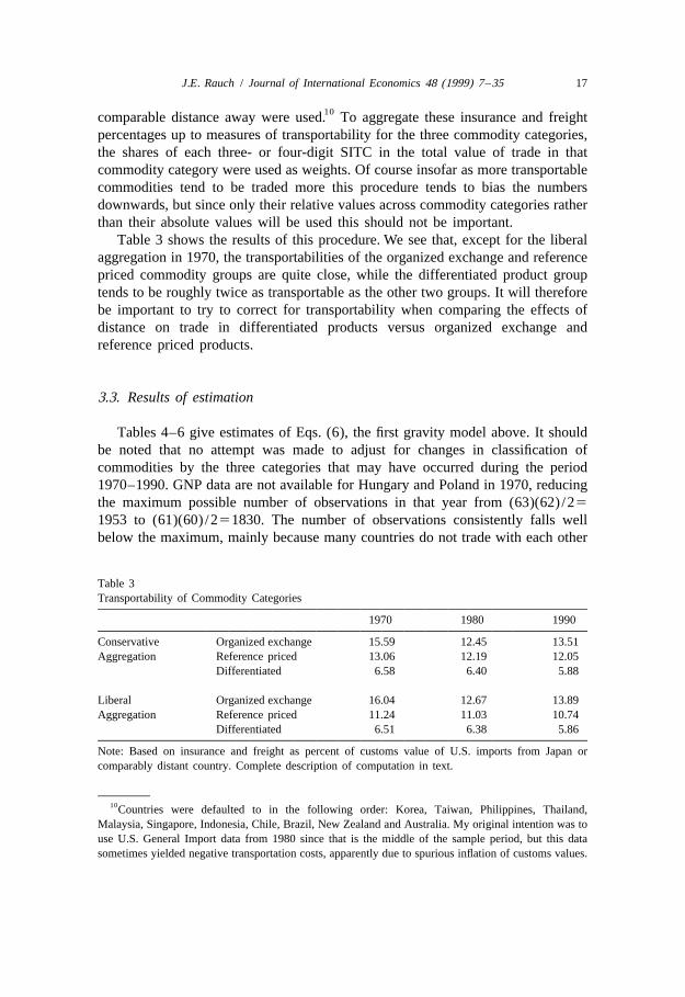
10comparable distance away were used. To aggregate these insurance and freightpercentages up to measures of transportability for the three commodity categories,the shares of each three- or four-digit SITC in the total value of trade in thatcommodity category were used as weights. Of course insofar as more transportablecommodities tend to be traded more this procedure tends to bias the numbersdownwards, but since only their relative values across commodity categories ratherthan their absolute values will be used this should not be important.
Table 3 shows the results of this procedure. We see that, except for the liberalaggregation in 1970, the transportabilities of the organized exchange and referencepriced commodity groups are quite close, while the differentiated product grouptends to be roughly twice as transportable as the other two groups. It will thereforebe important to try to correct for transportability when comparing the effects ofdistance on trade in differentiated products versus organized exchange andreference priced products.
3.3. Results of estimation
Tables 4–6 give estimates of Eqs. (6), the first gravity model above. It shouldbe noted that no attempt was made to adjust for changes in classification ofcommodities by the three categories that may have occurred during the period1970–1990. GNP data are not available for Hungary and Poland in 1970, reducingthe maximum possible number of observations in that year from (63)(62) /25
1953 to (61)(60) /251830. The number of observations consistently falls wellbelow the maximum, mainly because many countries do not trade with each other
Table 3Transportability of Commodity Categories
1970 1980 1990
Conservative Organized exchange 15.59 12.45 13.51Aggregation Reference priced 13.06 12.19 12.05
Differentiated 6.58 6.40 5.88
Liberal Organized exchange 16.04 12.67 13.89Aggregation Reference priced 11.24 11.03 10.74
Differentiated 6.51 6.38 5.86
Note: Based on insurance and freight as percent of customs value of U.S. imports from Japan orcomparably distant country. Complete description of computation in text.
10Countries were defaulted to in the following order: Korea, Taiwan, Philippines, Thailand,Malaysia, Singapore, Indonesia, Chile, Brazil, New Zealand and Australia. My original intention was touse U.S. General Import data from 1980 since that is the middle of the sample period, but this datasometimes yielded negative transportation costs, apparently due to spurious inflation of customs values.
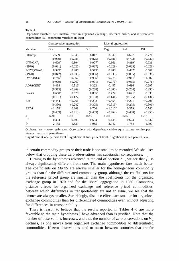
18 J.E. Rauch / Journal of International Economics 48 (1999) 7 –35
Table 4Dependent variable: 1970 bilateral trade in organized exchange, reference priced, and differentiatedcommodities (all continuous variables in logs)
Conservative aggregation Liberal aggregation
Variable Org. Ref. Dif. Org. Ref. Dif.
Intercept 22.509 25.948 28.817 23.340 26.627 28.774(0.939) (0.788) (0.825) (0.881) (0.772) (0.830)
a a a a a aGNP GNP 0.629 0.804 0.927 0.661 0.819 0.931i j
(1970) (0.031) (0.026) (0.027) (0.029) (0.025) (0.028)a a a a a aPGNP PGNP 0.349 0.485 0.573 0.408 0.497 0.567i j
(1970) (0.042) (0.035) (0.036) (0.039) (0.035) (0.036)a a a a a aDISTANCE 20.745 20.962 20.995 20.775 20.961 21.007
(0.079) (0.067) (0.071) (0.075) (0.065) (0.071)c bADJACENT 0.438 0.519 0.323 0.457 0.616 0.297
(0.315) (0.269) (0.288) (0.300) (0.264) 0.290)a a a a a aLINKS 0.650 0.626 0.895 0.724 0.671 0.839
(0.151) (0.127) (0.133) (0.141) (0.125) (0.134)cEEC 20.484 20.261 20.292 20.553 20.201 20.296
(0.330) (0.282) (0.305) (0.315) (0.275) (0.306)b bEFTA 21.178 0.208 0.700 21.010 0.379 0.740
(0.489) (0.418) (0.453) (0.467) (0.408) (0.455)n 1430 1510 1623 1501 1492 1617
2R 0.394 0.603 0.634 0.448 0.624 0.632s 2.135 1.829 1.985 2.042 1.784 1.997
Ordinary least squares estimation. Observations with dependent variable equal to zero are dropped.Standard errors in parentheses.a b cSignificant at one percent level. Significant at five percent level. Significant at ten percent level.
in certain commodity groups or their trade is too small to be recorded. We shall seebelow that dropping these zero observations has substantial consequences.
ˆTurning to the hypotheses advanced at the end of Section 3.1, we see that b isk
always significantly different from one. The main hypotheses fare much better.The coefficients on LINKS are always smaller for the homogeneous commoditygroups than for the differentiated commodity group, although the coefficients forthe reference priced group are smaller than the coefficients for the organizedexchange group in 1970 and for the liberal aggregation in 1980. Comparingdistance effects for organized exchange and reference priced commodities,between which differences in transportability are not an issue, we see that theformer are always smaller. Surprisingly, distance effects are smaller for organizedexchange commodities than for differentiated commodities even without adjustingfor differences in transportability.
There is reason to believe that the results reported in Tables 4–6 are morefavorable to the main hypotheses I have advanced than is justified. Note that thenumber of observations increases, and thus the number of zero observations on Vijk
declines, as one moves from organized exchange commodities to differentiatedcommodities. If zero observations tend to occur between countries that are far

J.E. Rauch / Journal of International Economics 48 (1999) 7 –35 19
Table 5Dependent variable: 1980 bilateral trade in organized exchange, reference priced, and differentiatedcommodities (all continuous variables in logs)
Conservative aggregation Liberal aggregation
Variable Org. Ref. Dif. Org. Ref. Dif.
Intercept 24.220 27.039 29.906 25.458 27.041 210.332(1.027) (0.729) (0.754) (0.928) (0.731) (0.763)
a a a a a aGNP GNP 0.816 0.859 0.918 0.824 0.898 0.915i j
(1980) (0.033) (0.023) (0.024) (0.030) (0.023) (0.024)c a a a a aPGNP PGNP 0.072 0.286 0.400 0.144 0.260 0.414i j
(1980) (0.039) (0.027) (0.028) (0.035) (0.027) (0.028)c a a a a aDISTANCE 20.617 20.809 20.764 20.595 20.874 20.742
(0.076) (0.054) (0.056) (0.069) (0.054) (0.057)a a b a a bADJACENT 0.842 0.658 0.540 0.787 0.616 0.592
(0.319) (0.231) (0.244) (0.292) (0.232) (0.247)a a a a a aLINKS 0.621 0.858 0.938 0.775 0.711 0.960
(0.158) (0.112) (0.115) (0.143) (0.112) (0.116)EEC 20.061 0.194 0.065 20.126 0.152 0.106
(0.333) (0.244) (0.257) (0.308) (0.241) (0.261)c cEFTA 20.676 0.332 0.688 20.362 0.519 0.708
(0.504) (0.369) (0.391) (0.467) (0.364) (0.395)n 1544 1662 1772 1628 1629 1772
2R 0.385 0.631 0.658 0.441 0.646 0.654s 2.215 1.623 1.721 2.053 1.603 1.742
Ordinary least squares estimation. Observations with dependent variable equal to zero are dropped.Standard errors in parentheses.a b cSignificant at one percent level. Significant at five percent level. Significant at ten percent level.
apart and do not share a common language/colonial tie, then omitting them willtend to reduce the estimated effects of DISTANCE and LINKS, and that reductionwill be greatest for organized exchange commodities and least for differentiated
11commodities. With this in mind we turn to Tables 7–9, which give the estimates12of Eqs. (8), the second gravity model above.
I find these estimates to be preferable on two grounds. First, they fit the gravityˆmodels of Section 3.1 better in the sense that b is never significantly differentk
from one in 1990, is significantly different from one only for organized exchangecommodities in 1980, and is not significantly different from one for differentiated
11Observations are missing in these tables because sometimes both country i and country j did notreport trade at all (or did not report trade with each other in the case of China and Taiwan), making itimpossible to reconstruct trade between them. This mainly happened in 1990 due to lags in reporting.
12Because the estimates of the thresholds a are positive (and statistically significant at the onek
percent level), the estimates of the coefficients b , g , and d converge only asymptotically to thek k k
estimated elasticities of the dependent variable with respect to the corresponding independent variablesas the dependent variable approaches infinity. The estimated elasticities evaluated at the mean values of
] ]kˆthe dependent variables can be found by multiplying the coefficient estimates by (a 1V ) /V , aijk ijk
quantity that never exceeds 1.001.

20 J.E. Rauch / Journal of International Economics 48 (1999) 7 –35
Table 6Dependent variable: 1990 bilateral trade in organized exchange, reference priced, and differentiatedcommodities (all continuous variables in logs)
Variable Conservative aggregation Liberal aggregation
Org. Ref. Dif. Org. Ref. Dif.
Intercept 21.417 24.480 28.013 22.124 24.720 28.174(0.932) (0.655) (0.647) (0.842) (0.665) (0.656)
a a a a a aGNP GNP 0.790 0.875 0.960 0.814 0.901 0.954i j
(1990) (0.031) (0.022) (0.021) (0.028) (0.022) (0.022)b a a a aPGNP PGNP 20.066 0.099 0.198 20.031 0.088 0.216i j
(1990) (0.033) (0.023) (0.022) (0.030) (0.023) (0.023)a a a a a aDISTANCE 20.701 20.830 20.754 20.707 20.858 20.765
(0.074) (0.052) (0.052) (0.067) (0.053) (0.053)a a a a a aADJACENT 1.223 1.016 0.945 1.163 1.015 0.952
(0.309) (0.224) (0.225) (0.283) (0.227) (0.228)a a a a a aLINKS 0.425 0.660 0.866 0.598 0.604 0.875
(0.153) (0.108) (0.107) (0.138) (0.110) (0.108)EEC 0.201 0.058 0.030 0.106 0.023 0.039
(0.329) (0.240) (0.241) (0.302) (0.243) (0.244)EFTA 21.148 20.108 0.150 0.110 20.005 0.138
(0.498) (0.362) (0.365) (0.457) (0.368) (0.370)n 1603 1724 1804 1667 1725 1795
2R 0.416 0.668 0.723 0.481 0.670 0.720s 2.175 1.587 1.603 2.000 1.612 1.622
Ordinary least squares estimation. Observations with dependent variable equal to zero are dropped.Standard errors in parentheses.a b cSignificant at one percent level. Significant at five percent level. Significant at ten percent level.
commodities in 1970. Second, the estimates show a consistent, if slight, ‘shrinkingof the globe’ that we would expect to observe given the improvements incommunication and transportation that occurred between 1970 and 1990. All ofthe coefficients on DISTANCE decrease in absolute value from 1970 to 1980 andagain from 1980 to 1990, unlike in Tables 4–6 where they mostly increase in
13absolute value between 1980 and 1990. (In Tables 4–6 four of the sixcoefficients on LINKS are smaller in 1990 than in either 1980 or 1970 while this is
14true for five out of six in Tables 7–9.).
13As distance-sensitive costs fall as a percentage of all costs, elasticity with respect to distance itselffalls (in absolute value).
14On the other hand, all of the coefficients on ADJACENT increase dramatically from 1970 to 1980and again from 1980 to 1990. Another strange aspect of the behavior of the adjacency effects is thatwhen one splits the differentiated commodity group into more and less transportable subgroups, as I dobelow, the distance effect is larger for the less transportable group as expected but the adjacency effectis smaller, leading one to wonder how much transportability really affects the coefficients onADJACENT. Given the erratic behavior of these coefficients I thought it prudent to reestimate Tables7–9 omitting the variable ADJACENT and the (maximum of) 67 country pairs for which it equals one.There were no qualitative changes in any results pertaining to the main hypotheses, and the same‘shrinking of the globe’ is observed.

J.E.
Rauch
/Journal
ofInternational
Econom
ics48
(1999)7
–3521
Table 7Dependent variable: 1970 bilateral trade in organized exchange, reference priced, and differentiated commodities (all continuous variables in logs)
Variable Conservative aggregation Liberal aggregation
Org. Ref. Dif. Org. Ref. Dif.
Intercept 28.523 28.752 29.983 27.981 29.420 29.935(1.056) (0.907) (0.856) (0.999) (0.870) (0.864)
a a a a a aGNP GNP 0.841 0.878 1.034 0.832 0.904 1.038i j
(1970) (0.035) (0.029) (0.030) (0.033) (0.027) (0.030)a a a a a aPGNP PGNP 0.528 0.635 0.558 0.546 0.640 0.557i j
(1970) (0.047) (0.040) (0.039) (0.044) (0.039) (0.040)a a a a a aDISTANCE 20.876 21.075 21.097 20.893 21.087 21.117
(0.083) (0.069) (0.071) (0.078) (0.067) (0.071)ADJACENT 0.458 0.326 20.025 0.320 0.314 20.060
(0.322) (0.304) (0.311) (0.319) (0.301) (0.308)a a a a a aLINKS 1.050 0.851 1.102 1.051 0.799 1.069
(0.155) (0.140) (0.138) (0.144) (0.138) (0.139)a a b a b bEEC 20.688 20.433 20.377 20.757 20.411 20.386
(0.194) (0.172) (0.175) (0.187) (0.170) (0.177)c a c c aEFTA 20.759 0.261 0.961 20.719 0.432 0.996
(0.436) (0.248) (0.196) (0.381) (0.244) (0.198)a a a a a aThreshold 37.561 23.442 12.205 37.040 21.582 11.742
($US Thous.) (4.318) (2.911) (1.687) (4.484) (2.538) (1.618)Log Likelihood 215067.8 215228.0 216571.4 215948.1 214750.9 216440.7
Maximum likelihood estimation of threshold Tobit model.Eicker–White standard errors in parentheses. Number of observations 51829.a b cSignificant at one percent level. Significant at five percent level. Significant at ten percent level.

22J.E
.R
auch/
Journalof
InternationalE
conomics
48(1999)
7–35
Table 8Dependent variable: 1980 bilateral trade in organized exchange, reference priced, and differentiated commodities (all continuous variables in logs)
Variable Conservative aggregation Liberal aggregation
Org. Ref. Dif. Org. Ref. Dif.
Intercept 212.093 211.140 212.540 210.955 211.924 212.891(1.173) (0.812) (0.788) (1.035) (0.830) (0.800)
a a a a a aGNP GNP 1.130 1.000 1.028 1.072 1.038 1.026i j
(1980) (0.038) (0.025) (0.026) (0.034) (0.025) (0.026)a a a a a aPGNP PGNP 0.205 0.383 0.394 0.223 0.401 0.406i j
(1980) (0.047) (0.034) (0.033) (0.043) (0.034) (0.033)a a a a a aDISTANCE 20.852 20.923 20.761 20.806 20.981 20.745
(0.085) (0.062) (0.061) (0.077) (0.061) (0.061)b b bADJACENT 0.754 0.570 0.415 0.653 0.469 20.455
(0.349) (0.302) (0.312) (0.322) (0.319) (0.315)a a a a a aLINKS 1.056 1.040 1.139 1.025 0.948 1.154
(0.179) (0.140) (0.131) (0.163) (0.141) (0.131)c bEEC 20.364 0.010 0.172 20.436 20.049 0.208
(0.214) (0.159) (0.152) (0.197) (0.162) (0.154)b a a aEFTA 0.113 0.548 1.083 0.180 0.677 1.105
(0.512) (0.272) (0.234) (0.415) (0.257) (0.238)a a a a a aThreshold 134.085 114.518 89.170 150.067 112.123 81.416
($US Thous.) (16.387) (13.099) (12.557) (18.503) (12.970) (11.507)Log Likelihood 219323.5 219922.5 221903.8 220503.9 219391.9 221778.8
Maximum likelihood estimation of threshold Tobit model.Eicker–White standard errors in parentheses. Number of observations51951.a b cSignificant at one percent level. Significant at five percent level. Significant at ten percent level.

J.E.
Rauch
/Journal
ofInternational
Econom
ics48
(1999)7
–3523
Table 9Dependent variable: 1990 bilateral trade in organized exchange, reference priced, and differentiated commodities (all continuous variables in logs)
Variable Conservative aggregation Liberal aggregation
Org. Ref. Dif. Org. Ref. Dif.
Intercept 28.245 27.893 29.752 27.656 27.933 210.026(1.012) (0.673) (0.644) (0.903) (0.690) (0.654)
a a a a a aGNP GNP 1.048 0.993 1.025 1.011 1.006 1.030i j
(1990) (0.034) (0.023) (0.022) (0.031) (0.023) (0.023)a a a aPGNP PGNP 20.005 0.115 0.184 0.022 0.117 0.196i j
(1990) (0.036) (0.025) (0.023) (0.033) (0.024) (0.023)a a a a a aDISTANCE 20.784 20.808 20.714 20.743 20.851 20.732
(0.078) (0.055) (0.054) (0.070) (0.057) (0.054)a a a a a aADJACENT 1.761 1.343 1.155 1.609 1.330 1.164
(0.310) (0.246) (0.246) (0.277) (0.254) (0.249)a a a a a aLINKS 0.799 0.869 0.978 0.848 0.783 0.992
(0.169) (0.120) (0.116) (0.153) (0.123) (0.117)EEC 20.167 20.019 0.088 20.186 20.090 0.085
(0.207) (0.162) (0.157) (0.195) (0.160) (0.160)c cEFTA 0.090 0.079 0.351 0.263 0.110 0.359
(0.469) (0.226) (0.208) (0.355) (0.216) (0.214)a a a a a aThreshold 101.649 125.929 110.741 124.413 105.654 106.585
($US Thous.) (12.384) (16.083) (16.624) (15.118) (13.572) (15.576)Log Likelihood 219759.6 221225.8 223019.7 220836.8 221044.3 222794.3
Maximum likelihood estimation of threshold Tobit model.Eicker–White standard errors in parentheses. Number of observations51925.a b cSignificant at one percent level. Significant at five percent level. Significant at ten percent level.

24 J.E. Rauch / Journal of International Economics 48 (1999) 7 –35
Turning to the main hypotheses, the coefficients on LINKS are always less forthe homogeneous commodity groups than for the differentiated commodity group,but the coefficients for the reference priced group are always less than thecoefficients for the organized exchange group, except for the conservative
15aggregation in 1990. The most important change from Tables 4–6 is that thedifferences between the organized exchange group coefficients and the differen-tiated group coefficients are much smaller. Comparing distance effects fororganized exchange and reference priced commodities, we see that as in Tables
164–6 the former are always smaller. Unlike in Tables 4–6, however, distanceeffects are larger for the homogeneous commodity groups than for the differen-tiated commodity group except in 1970.
Since Table 3 indicates that differentiated commodities are roughly twice astransportable as organized market or reference priced commodities, adjustment ofthe distance coefficients for differentiated products is in order. The simplest way todo this is to estimate the sensitivity of these coefficients to differences intransportability within differentiated commodities, and use this estimate tocompute what the coefficients would have been had differentiated commoditiesbeen as transportable as either organized market or reference priced commodities.To avoid greatly increasing the number of observations for which V 50 whenijk
producing this estimate, I simply split differentiated commodities at the medianvalue of transportability into more and less transportable groups, and then estimatethe gravity equation separately for each group. The resulting distance coefficientsare reported in Table 10, where l denotes the less transportable group and mdenotes the more transportable group.
The adjustment of the distance coefficients for differentiated commodities inTables 7–9 then proceeds as follows. Assume that the distance coefficients d areadditively separable functions of search costs and transportation costs. Maintainingthe hypothesis that search costs are equal within a commodity category, d 2dl m
leaves only the difference attributable to less versus more transportability. Nowdenote our measure of transportability by t, and denote measures computed as inTable 3 for the less transportable group of differentiated products (t.median) andthe more transportable group (t#median) by t and t , respectively. If we choosel m
the functional form c ln t for the transportation cost component of d, d 2d yieldsl m
c ln(t /t ) so that only relative values of t will matter in the adjustments. We thusl m
compute our estimate of c, the sensitivity of the distance coefficient fordifferentiated commodities to differences in transportability, using the formula
15Omitting Petroleum from the organized exchange group yields the following coefficients on LINKSfor 1970, 1980, and 1990, reporting the conservative and liberal aggregations respectively: 1.170 and1.150, 1.141 and 1.093, 0.827 and 0.874.
16Omitting Petroleum from the organized exchange group yields the following coefficients onDISTANCE for 1970, 1980, and 1990, reporting the conservative and liberal aggregations respectively:20.678 and 20.730, 20.666 and 20.648, 20.662 and 20.636.

J.E. Rauch / Journal of International Economics 48 (1999) 7 –35 25
Table 10Computation of transportability adjustments for differentiated commodity distance coefficients
1970 1980 1990
Con. Lib. Con. Lib. Con. Lib.
d 21.136 21.126 20.911 20.877 20.855 20.857l
d 21.004 21.044 20.659 20.651 20.643 20.655m
t 9.66 9.45 9.78 9.60 9.51 9.31l
t 4.05 4.03 3.90 3.89 3.81 3.76m
c 20.152 20.096 20.274 20.250 20.232 20.223ˆAdjusted d
for comparison to:organized exchange 21.228 21.204 20.943 20.917 20.907 20.924
[20.876] [20.893] [20.852] [20.806] [20.784] [20.743]reference priced 21.201 21.169 20.938 20.882 20.881 20.867
[21.075] [21.087] [20.923] [20.981] [20.808] [20.851]
Con.5‘Conservative’ aggregation. Lib.5‘Liberal’ aggregation. d 5distance coefficient. t5transportability. l(m)5less (more) transportable differentiated commodity group. c5sensitivity ofdistance coefficient for differentiated commodities to differences in transportability. Bracketedcoefficient estimates are repeated from Tables 7–9 for convenience.
ˆ ˆ(d 2 d / ln(t /t ). We can then compute what the distance coefficients forl m l m
differentiated commodities in Tables 7–9 would have been had their transportabili-ty been equal to that of organized exchange commodities and reference priced
ˆ ˆcommodities, respectively, by adding c ln(t /t ) and c ln(t /t ) to these coeffi-1 3 2 3
cients, where t are the appropriate numbers from Table 3. The results are reportedk
at the bottom of Table 10.With the exception of the liberally aggregated reference priced commodities in
1980, the adjusted distance effects for differentiated commodities are larger thanthe distance effects for the homogeneous commodity groups. Note that byconstruction the differences between the coefficients at the bottom of Table 10 andthe coefficients on DISTANCE in Tables 7–9 for organized exchange commoditiesand reference priced commodities are equal to the differences in the searchcomponents of these coefficients.
While the evidence presented in this section supports the hypotheses thatproximity and common language/colonial ties are more important in matchinginternational buyers and sellers of differentiated products than homogeneousproducts, and also the hypothesis that proximity is least important for homoge-neous products traded on organized exchanges, it does so only weakly. Thedifferences in the coefficients on DISTANCE and LINKS are consistent in sign butsmall in absolute magnitude. Focusing on the conservative aggregation, in absolutevalue the adjusted elasticities of differentiated products trade with respect toDISTANCE reported in Table 10 range from 10.6 percent (in 1980) to 40.0 percent(in 1970) greater than the elasticities of organized exchange product trade andfrom 1.6 percent (in 1980) to 11.7 percent (in 1970) greater than the elasticities of
26 J.E. Rauch / Journal of International Economics 48 (1999) 7 –35
17reference priced product trade. The extent to which LINKS increases bilateraldifferentiated products trade ranges from 5.1 percent (in 1970) to 19.5 percent (in1990) greater than the extent to which it increases bilateral organized exchangeproduct trade and from 10.3 percent (in 1980) to 28.5 percent (in 1970) greaterthan the extent to which it increases bilateral reference priced product trade.
More formally, comparing within each year the coefficients on DISTANCE (asadjusted in Table 10) and LINKS for differentiated products to the correspondingcoefficients for the two homogeneous commodity groups makes a total of sixcomparisons each for DISTANCE and LINKS for a given aggregation. Continuingto focus on the conservative aggregation, a nonparametric sign test rejects thehypothesis that the median of the differences between the six pairs of coefficientsis zero at the five percent level for both the (adjusted) coefficients on DISTANCEand the coefficients on LINKS. On the other hand, it seems unlikely in most casesthat we could reject the hypothesis that the difference between any particular pairof coefficients equals zero. Rather than estimate a nonlinear version of a seeminglyunrelated regressions (SUR) model to verify this statement, for computationalsimplicity we estimate a SUR model for each year using ln(11V ) as theijk
dependent variables. Although of course this yields coefficient estimates differentthan those reported in Tables 7–9, the ratio of the differences between thecoefficients to their standard errors is quite similar. Only for the coefficients onDISTANCE for organized exchange products in 1970 and LINKS for referencepriced products in 1970 can we reject (at the five percent level) the hypothesis thatthe difference from the corresponding coefficient for the differentiated commoditygroup is zero, where the adjustments to the coefficients on DISTANCE for
18differentiated products have been treated as deterministic. The implications ofthis weak evidence in favor of its key predictions for the value of the network /search approach to trade in differentiated products will be discussed in theconcluding section of this paper.
4. Evidence from the OECD COMTAP database
In the previous section we considered evidence for the network/search view oftrade in differentiated products that could be revealed by the contrast between theway countries matched up in international trade in these products versus more
17The correction in footnote 12 was applied in making these computations.18 ˆIf we estimate c in Table 10 using ln(11V ) as the dependent variables we can also reject (at theijk
five percent level) the hypothesis that the difference between the coefficient on DISTANCE forreference priced products in 1970 and the corresponding coefficient for the differentiated commoditygroup is zero.

J.E. Rauch / Journal of International Economics 48 (1999) 7 –35 27
homogeneous products, especially those traded on organized exchanges. This viewalso has implications for the extent to which differentiated versus homogeneousproducts are traded at all, that is, for the shares of production of different productsthat are traded rather than supplied or consumed domestically. Let us consider acommodity that is sufficiently homogeneous to have a reference price, but forwhich no trader is able to keep sufficiently informed of prices around the world toengage in international commodity arbitrage. We suppose therefore that any traderwho wishes to export (import) this commodity must search for a price that issufficiently higher (lower) than the domestic price to cover transportation, tariffs,and so on. I claim that this search will be much less costly than a search for buyers(sellers) of a differentiated product that are good ‘matches’, because prices canvary along only one dimension while product characteristics can vary along many.Hence the barrier to trade in products with reference prices is smaller than thebarrier to trade in differentiated products, ceteris paribus, and we expect a higherproportion of production of the former products to be exported and a higherproportion of their consumption to be imported.
To test this hypothesis we need data on trade that is matched with data onproduction. Unfortunately, trade data is collected according to the StandardInternational Trade Classification while production data is collected according tothe International Standard Industrial Classification (ISIC). The Compatible Tradeand Production Database (see Berthet-Bondet et al., 1988, for a description)converts trade data to an ISIC basis for the period 1970–1985 for the OECD only,and only for manufacturing industries (ISIC codes beginning with 3). Productiondata is disaggregated to the four-digit ISIC level only for 13 of the 22 OECDcountries, which however account for 95.1 percent and 94.0 percent of total OECD
19manufacturing production in 1970 and 1985, respectively. A total of 82 industriesare distinguished, of which one, Metal Scrap from Manufacture of FabricatedMetal Products (ISIC 3801), had to be dropped due to fragmentary data. Theanalysis below is therefore based on the total production, exports, and imports ofthe 13 reporting OECD countries for 81 manufacturing industries.
Using OECD data presents a problem that would not occur if we had data forthe entire world, for which imports are identically equal to exports: it might matterwhether we test the hypothesis that tradedness increases with reference pricingusing the export share of production or the import share of consumption. Inparticular, the OECD tends to have a comparative advantage relative to the rest ofthe world in differentiated manufactures and a comparative disadvantage inhomogeneous manufactures, perhaps because the former are more skill-intensiveor technologically sophisticated, leading to a bias against my hypothesis whentested using the export share of production and in favor of my hypothesis when
19The 13 countries are Australia, Belgium–Luxembourg, Canada, Finland, France, Italy, Japan,Netherlands, Norway, Sweden, United Kingdom, United States, and West Germany.
28 J.E. Rauch / Journal of International Economics 48 (1999) 7 –35
tested using the import share of consumption. I decided to simply use the average20of the export share and the import share as my dependent variable:
SHARE ; [Exports /Production
1 Imports /(Production 1 Imports 2 Exports)] /2 .
The computation of the percentage of each industry’s output that is referencepriced is complicated by the fact that production figures for more disaggregatedlevels of the ISIC are not available. I therefore used the 1979 U.S. Department ofCommerce publication Correlation Between the United States and InternationalStandard Industrial Classifications to match each ISIC to the correspondingfour-digit U.S. SIC(s), and then classified each seven-digit U.S. SIC component asreference priced or not. I then aggregated up from the seven-digit level usingoutput figures from the 1977 U.S. Census of Manufactures to estimate thepercentage of each ISIC’s output that is reference priced, where 1977 was chosenbecause it is the midpoint of the period covered by the COMTAP database. For thepurposes of this section I chose to use this estimate as a continuous explanatory
21variable rather than to classify each industry as reference priced or not.Transportability was estimated using the difference between c.i.f. and customs
values of U.S. imports as in the previous section. Since the U.S. Department ofCommerce does not produce trade data classified by ISIC, the transportabilityestimate for the largest U.S. SIC among those that make up the 4-digit ISIC wasused. Where the largest was not available (e.g., because the Department ofCommerce does not use it to record trade), a judgment was made concerning theSIC that is most representative of the ISIC.
Since our estimates of transportability and reference pricing do not change fromyear to year, estimation will be reported for the beginning and end years of thesample only. (Results are not qualitatively different for other years.) Table 11gives descriptive statistics for transportability (TRANSPORT ), reference pricing(PRICING), and SHARE. Note that the median for reference pricing is less thantwo percent: most manufacturing industries have essentially no reference pricing,indicating that the zero-one classification of commodities as reference priced ornot in the previous section was not such a bad approximation, at least for
20In 1970 the average of the export share of production across 81 commodities was 13.8 percentcompared to 12.6 percent for the import share of consumption. The comparable figures for 1985 were19.0 percent and 18.9 percent. Hence there is no comparative advantage revealed for the OECD relativeto the rest of the world in manufacturing as a whole. However, the average absolute difference betweenthe two shares was 3.3 percent in 1970 and 4.2 percent in 1985. Clearly these figures would be muchlarger if the OECD did not mostly trade with itself.
21As mentioned above, reference pricing is typically based on the availability of price quotations inU.S. trade publications based on surveys of U.S. wholesale markets. It follows that there is minimalscope for ‘reverse causation’, where extensive international trade leads to more price quotation and ahigh estimate of reference pricing.

J.E. Rauch / Journal of International Economics 48 (1999) 7 –35 29
Table 11Descriptive statistics for Table 12
Variable Mean Std Dev Median Min Max
TRANSPORT 0.084 0.045 0.075 0.013 0.289PRICING 0.235 0.335 0.016 0.000 1.0001970 SHARE 0.132 0.107 0.116 0.005 0.7041985 SHARE 0.190 0.131 0.161 0.017 0.757
All variables have 81 observations except 1985 SHARE, which has 80 due to exclusion of ISIC 3232. IfISIC 3232 is excluded from TRANSPORT and PRICING, the mean, standard deviation, and medianrespectively change to 0.238, 0.336, and 0.020 for PRICING, and only change in the fourth decimalplace for TRANSPORT. The minimums and maximums remain unchanged.
manufactured commodities. The minimum and maximum for TRANSPORTcorrespond to Aircraft (ISIC 3845) and Cement, Lime, and Plaster (ISIC 3692),respectively. A comparison of the 1970 and 1985 values of SHARE shows asubstantial increase in OECD openness during this period, as expected. I alsocomputed simple and rank correlation coefficients between TRANSPORT andPRICING, obtaining 0.490 and 0.460, respectively. These results are also in linewith expectations.
22Table 12 reports regressions of SHARE on TRANSPORT and PRICING.Because SHARE can only vary from zero to one but OLS can yield predictionsoutside this range, a logistic transformation of SHARE is used as the dependent
Table 12Dependent variable: Ln [SHARE /(12SHARE)], reporting OECD countries, 4-digit manufacturingISICs
Variable 1970 1970 1985 1985
Intercept 21.199 20.458 20.828 20.080(0.206) (0.425) (0.212) (0.428)
a a a aTRANSPORT 213.32 213.19 210.89 29.593(2.483) (2.901) (2.537) (2.935)
a bPRICING 0.533 1.297 0.133 0.942(0.331) (0.370) (0.338) (0.373)
2-digit ISIC dummies included? NO YES NO YESn 81 81 80 80
2R 0.279 0.464 0.224 0.440s 0.864 0.786 0.882 0.792Dependent mean: 22.186 22.186 21.711 21.711
a bStandard errors in parentheses. Significant at one percent level. Significant at five percent level.
22Use of the logarithm of TRANSPORT leaves the results qualitatively unchanged.

30 J.E. Rauch / Journal of International Economics 48 (1999) 7 –35
23variable. The results in the first and third columns are not favorable to thehypothesis that reference pricing reduces barriers to trade: TRANSPORT has arobustly negative effect on SHARE while the effect of reference pricing isstatistically insignificant. It may be, however, that the effect of reference pricingon tradeability is being masked by industry characteristics that are correlated withreference pricing and affect tradeability but are not picked up by TRANSPORT.For example, concern with ‘freshness’ may act as a barrier to trade forManufacturing of Food, Beverages, and Tobacco (ISIC 31). To account for thispossibility, eight dummy variables for ISIC 31–38 (ISIC 39 is the omittedtwo-digit industry) are included in the second and fourth columns of Table 12.F-tests reject exclusion of these dummies at the one percent level in both 1970 and1985. We see that reference pricing does have a statistically significant effect onSHARE within a two-digit manufacturing industry.
How important is reference pricing in lowering barriers to trade within atwo-digit industry? Holding all other variables (including dummies) at their meanlevels, we can compute the predicted value of SHARE for an industry with zeroreference pricing and one hundred percent reference pricing using the formula
ˆ ˆ ˆexp(y ) / [11exp(y )], where y is the predicted value of the transformed dependentvariable. The results are 0.077 and 0.233 in 1970 and 0.126 and 0.270 in 1985,indicating that a change from no reference pricing to full reference pricing morethan doubles the tradedness of an industry within a two-digit classification. Thedecrease in the effect of reference pricing between 1970 and 1985 is consistentwith the ‘shrinking of the globe’ found in the previous section. A similar decrease(in absolute value) is found for the effect of transportability within a two-digitindustry: the elasticity of SHARE with respect to TRANSPORT, evaluated at themeans, equals 20.96 in 1970 and 20.65 in 1985.
5. Alternative explanations
I have examined evidence at the level of world trade flows in order to determinewhether the theoretical considerations of Section 2 make a difference at theaggregate level. Too often, the effects of imperfect information are discussed onlyat the micro level, with no sense of how or if they aggregate up to somethingobservable at the macro level. Unfortunately, evidence at such an aggregate levelallows for many alternative explanations. This evidence will ultimately have to besupplemented by case studies of trading and marketing practices for different typesof products.
23The transformation is ln[SHARE /(12SHARE)]. In 1985 the value of exports for Fur Dressing andDyeing Industries (ISIC 3232) exceeded the value of production, presumably because of difficulties intranslating from SITC to ISIC. I therefore dropped this industry, leaving 80 observations. Simplysubstituting imports for exports and retaining this observation does not qualitatively change the results.

J.E. Rauch / Journal of International Economics 48 (1999) 7 –35 31
Many of the alternative explanations for the results in Section 3 and Section 424can explain only some of the results. Rather than try to discuss each one (and
knowing that the reader can always think of more), I will discuss one alternativeexplanation that I find particularly compelling because it can explain all of the
25results. Suppose that firms develop their varieties of differentiated products tosuit niches in their home markets. We suppose further that they do this not becausethey know more about their home markets than about foreign markets, whichwould again indicate an incomplete information structure where information aboutbuyers is mediated by distance, but because positive transportation costs make thisthe best decision, ceteris paribus. This could explain why differentiated productstend to be less traded: there is less demand for them outside the country in whichthey are produced. Now suppose further that the similarity of foreign preferencesto those in the home country falls with distance and rises with common language /colonial ties. This could explain why trade in differentiated products decreasesmore with distance and increases more with links than trade in homogeneous
26products: a geographic and linguistic application of the Linder hypothesis.Two pieces of evidence can be brought to bear on the validity of this alternative
explanation. First, recall that the LINKS variable used by Frankel et al. (1993)equals one if a pair of countries shares either a colonial tie or a common language.Comparing colonial ties to common language, it is plausible that the former wouldbe relatively more important as an indicator of preexisting business ties while thelatter would be relatively more important as an indicator of taste similarity.Suppose that we separate LINKS into dummy variables for colonial ties andcommon language. If the alternative explanation has merit, at a minimum wemight expect an increase (decrease) relative to the coefficients on LINKS in theextent to which the coefficients on the common language (colonial ties) dummy
24A good example is based on the natural resource intensity of organized exchange and referencepriced products. It can be argued that this leads these products to be traded more extensively, andacross greater distances (Kuwait and Saudi Arabia should not exchange much petroleum), but thisalternative explanation cannot explain the lower coefficients on LINKS for these product groups. In anycase, this argument should hold most strongly for countries that share a land border, yet the coefficientson ADJACENT in Tables 7–9 are always largest for organized exchange products and smallest fordifferentiated products. The fact that the coefficient on DISTANCE falls (in absolute value) whenpetroleum is omitted from the organized exchange group (see footnote 16) also casts doubt on thisalternative explanation.
25On the other hand, there may be reasons to believe that the results would be stronger in the absenceof certain countervailing influences. For example, we know that there are many preferential tradingagreements for agricultural products based on colonial ties, and these should work to make the linkseffect larger for the homogeneous commodity groups.
26Of course production of similar varieties in nearby countries and countries with a commonlanguage/colonial tie would increase too, but this may just stimulate ‘intraindustry’ trade rather thandecreasing trade. Moreover, this production of similar varieties allows extension of the alternativeexplanation to trade in producer goods as well as consumer goods.

32 J.E. Rauch / Journal of International Economics 48 (1999) 7 –35
are larger for differentiated commodities than for the homogeneous commoditygroups.
A colonial ties dummy variable was constructed on the basis of articles in theEncyclopedia Britannica, 1997. A common language dummy variable wasconstructed by assigning countries to language groups on the basis of Ethnologue
27(Grimes, 1984). (LINKS can be recovered from the two new variables by takingtheir sum and setting its value equal to one whenever it equals two.) The results ofreestimating Tables 7–9 provide surprisingly strong evidence against the alter-native explanation (details are available on request). The coefficients on commonlanguage are never positive and significant except for the conservatively andliberally aggregated reference priced commodities in 1990. The coefficients oncolonial ties are always positive, significant, and largest for the differentiatedcommodity group in every year for both aggregations. The absolute differences ofthe differentiated from the homogeneous commodity group coefficients are greaterthan those reported in Tables 7–9 for LINKS in every case except for the liberallyaggregated reference priced commodities in 1980 and the conservatively aggre-gated organized exchange commodities in 1990.
The second piece of evidence is a clever study by Gould (1994). He finds thatimmigration to the United States increases U.S. bilateral trade with the im-migrants’ countries of origin, that this ‘immigrant-link effect’ is stronger for U.S.exports than for U.S. imports, and that the effect on exports exhausts itself for amuch smaller number of immigrants than does the effect on imports. Takentogether these results indicate that the most important effect of immigration ontrade is through the establishment of business contacts, with a secondary effectthrough increased U.S. preferences for goods produced in the country of origin. Byextension, the argument that preferences are mainly responsible for the findings ofSection 3 and Section 4 is undermined.
If the theory of Section 2 has merit, the immigrant-link effect on trade should begreatest for differentiated products and smallest for homogeneous products tradedon organized exchanges. Gould did in fact disaggregate his dependent variable,U.S. trade in manufactures from 1970 to 1986 (from the OECD COMTAPdatabase used in Section 4 above), into what he called consumer and producergoods. The four-digit industries he lists in the former category tend to be less‘priced’ in the sense of Section 4 than those in the latter category. Gould reports
27Two countries were considered to belong to the same language group if at least ten percent of thepopulation of each country speaks that language at home. While colonial ties and common languageoften went together, in the majority of cases this was not true. For example, Belgium and France sharea common language, but not a colonial tie; Kenya and the UK share a colonial tie, but not a commonlanguage.
J.E. Rauch / Journal of International Economics 48 (1999) 7 –35 33
(p. 310) that, ‘The immigrant information variable does not appear to be important28in the producer imports equation.’
6. Conclusions and suggestions for further research
In Section 3 we saw that the differences in proximity and links effects acrossorganized exchange, reference priced, and differentiated commodities, while in thedirection predicted by the network/search view of trade in differentiated products,were quantitatively small. In Section 4 we saw that the effects of reference pricingon the extent of trade were present only within a two-digit industry. Are theseresults due to a small quantitative importance of networks and search in trade, orto an overestimation of the importance of ‘markets’, leading to networks andsearch being very significant for homogeneous as well as differentiated products?The latter explanation is supported by the fact that the coefficients on LINKSconsistently imply that countries that share a common language/colonial tie tradewith each other products listed on organized exchanges more than twice as much
29as countries that do not. Once again, however, examination of more disaggre-gated data or even case studies of trader behavior will ultimately be needed toanswer this question.
An important aim of this paper is to put networks and search on the agenda forthe study of trade. One advantage of the network/search view of trade indifferentiated products is that it helps to make sense of certain microinstitutionalfeatures of trade. In Rauch (1996) I show that a simple partial equilibrium searchmodel yields economies of scope in search for buyers of differentiated products,which can help us understand the role of ‘social capital’ in international trade andthe viability of general trading companies such as Japan’s sogo shosha. I also notethat if search is subject to free-riding (through unintended information spillover)there may be a rationale for widely observed export promotion policies such assubsidized trade missions. More broadly, the network/search view of trade opensup space for greater consideration of the role of personal contacts and relationship-building in determining the geographic distribution of economic activity. This is
28When Gould uses the logarithm of the immigrant stock as his explanatory variable, yielding aconstant elasticity specification (also used by Head and Ries, 1996, in their work on immigration andtrade for Canada), it is significant in the consumer export equation but not in the equations forconsumer or producer imports or producer exports. It should be noted that Gould’s equations containfixed effects for every U.S. trading partner, so the immigrant stock cannot be acting as a proxy fordistance or common language/colonial ties.
29Since the value of this trade is dominated by grains, oil seeds, fuels, and both mineral andnonmineral raw materials such as metals, a preference-based explanation for this finding is highlyimplausible.

34 J.E. Rauch / Journal of International Economics 48 (1999) 7 –35
the subject of many business press anecdotes but not much systematic economicanalysis (see Egan and Mody, 1992 for an exception).
Foreign Direct Investment (FDI) projects bear the same relationship to portfolioinvestments as differentiated products do to homogeneous products. Unfortunately,as far as I know it is impossible to obtain data on bilateral portfolio investmentflows, making comparisons of the kind performed in Section 3 impossible.Nevertheless, the importance of proximity for bilateral FDI flows could be seen asevidence in favor of the robustness of the network/search view as an approach tounderstanding economic transactions more generally, the transactions being in‘differentiated projects’ rather than differentiated products. Eaton and Tamura(1994) examine U.S. and Japanese bilateral FDI flows. They use regional dummiesrather than distance, and find (p. 4), ‘Taking into account population, income, andfactor endowments, both countries have deeper trade and investment relationshipswith countries in their respective regions than with the rest of the world.’ Thisfinding is especially striking when one considers that most FDI is undertaken withthe aim of penetrating the market of the host country, so that one should expectdistance to have a positive effect on bilateral FDI flows given the proximity-concentration tradeoff.
A long-term goal for future research is formalization of the network/searchview of trade in a general equilibrium model. It is possible that this could lead tomany more empirical applications and more detailed predictions. We may, forexample, be able to improve our analysis of the effects of distance and commonlanguage/colonial ties in mediating the economic impacts of trade liberalization
30agreements.
Acknowledgements
This paper has benefited from discussions with Ross Starr. Comments byJonathan Eaton, Walter Heller, and two anonymous referees have also beenhelpful. I wish to thank James Harrigan and Shang-Jin Wei for generouslysupplying data and Donald McCubbin for outstanding research assistance.Previous drafts were presented at the National Bureau of Economic Research, theWorld Bank, and the following universities: British Columbia, Rice, Texas atAustin, California at Los Angeles, City of New York Graduate Center, Princeton,New York, Maryland at College Park, Harvard, Columbia, Queens College of Cityof New York, and Brown. Financial support was provided by NSF grant [SBR94-15480. I am responsible for any errors.
30Leamer (1993), pp. 60–61, concluded that, ‘NAFTA is not a free trade agreement between Canada,the United States, and Mexico. It is really a free trade agreement between northern Mexico, California,and Texas.’

J.E. Rauch / Journal of International Economics 48 (1999) 7 –35 35
References
Berthet-Bondet, C., Blades, D., Pin, A., 1988. The OECD Compatible Trade and Production Data Base1970–1985. OECD Department of Economics and Statistics, Working Paper No. 60, November.
Deardorff, A.V., 1995. Determinants of bilateral trade: Does gravity work in a neoclassical world?National Bureau of Economic Research, Working Paper No. 5377, December.
Eaton, J., Tamura, A., 1994. Bilateralism and regionalism in Japanese and U.S. trade and direct foreigninvestment patterns. Journal of the Japanese and International Economies 8, 478–510.
Egan, M.L., Mody, A., 1992. Buyer–seller links in export development. World Development 20,321–334.
Encyclopedia Britannica, 1997. Internet Edition.Frankel, J., Stein, E., Wei, S., 1993. Continental trading blocs: Are they natural, or supernatural?
National Bureau of Economic Research, Working Paper No. 4588, December.Gereffi, G., Korzeniewicz, M., 1990. Commodity chains and footwear exports in the semiperiphery. In:
Martin, W. (Ed.), Semiperipheral States in the World Economy. Greenwood, Westport CT, pp.45–68.
Gould, D.M., 1994. Immigrant links to the home country: Empirical implications for U.S. bilateraltrade flows. Review of Economics and Statistics 76, 302–316.
Grimes, B. (Ed.), 1984. Ethnologue: Languages of the world, 11th ed. Summer Institute of Linguistics,Dallas TX.
Hahn, F.H., 1971. Equilibrium with transaction costs. Econometrica 39, 417–439.Harrigan, J., 1994. Scale economies and the volume of trade. Review of Economics and Statistics 76,
321–328.Head, K., Ries, J., 1996. Immigration and trade creation: Econometric evidence from Canada. Faculty
of Commerce, University of British Columbia, March.Heller, W.P., 1993. Equilibrium market formation causes missing markets. University of California, San
Diego, Discussion Paper No. 93-07, February.Helpman, E., 1987. Imperfect competition and international trade: Evidence from fourteen industrial
countries. Journal of the Japanese and International Economies 1, 62–81.Hummels, D., Levinsohn, J., 1995. Monopolistic competition and international trade: Reconsidering the
evidence. Quarterly Journal of Economics 110, 799–836.Leamer, E.E., 1993. U.S. Manufacturing and an emerging Mexico. North American Journal of
Economics and Finance 4, 51–89.Nothdurft, W.E., 1992. Going global: How Europe helps small firms export. Brookings Institution,
Washington D.C.Rauch, J.E., 1996. Trade and search: Social capital, sogo shosha, and spillovers. National Bureau of
Economic Research, Working Paper No. 5618, June.Rozanski, J., Yeats, A., 1994. On the (in)accuracy of economic observations: An assessment of trends
in the reliability of international trade statistics. Journal of Development Economics 44, 103–130.