Network Optimization

Network optimization models:Special cases of linear programming models

Important to identify problems that can be modeledas networks because:

(1) network representations make optimizationmodels easier to visualize and explain

(2) very efficient algorithms are available

Example of (Distribution) Network

8

5

6

4

2

7

3

1

(6)

(3)

(5)

(7)

(4)

(2)

(4)(5)

(5)(6)

(4)

(7)

(6)

(3)

[-150]

[200]

[-300]

[200]

[-200]

[-200]

(2)

(2)

(7)

[-250]

[700]

[external flow] (cost)

lower = 0, upper = 200

1

2 34

5

6 7

108

911

12

13

14 15

16

17

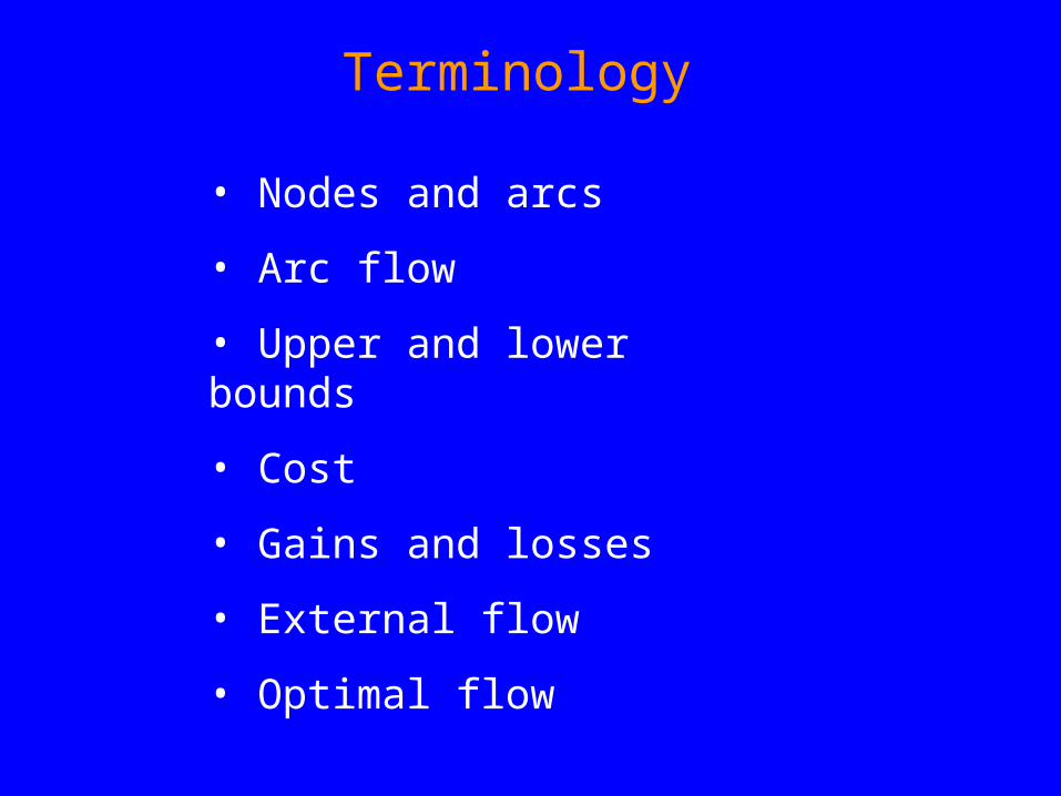
Terminology

• Nodes and arcs

• Arc flow

• Upper and lower bounds

• Cost

• Gains and losses

• External flow

• Optimal flow

Network Flow Problems

Pure Minimum

Cost Flow

Problem

Generalized Minimum

Cost Flow

Problem

Linear Program

Transportation Problem

Assignment Problem

Shortest Path Problem

Maximum Flow Problem

Less general models

More general models

Transportation Problem

We wish to ship goods (a single commodity) from m sources to n destinations at minimum cost.

Warehouse i has si units available i = 1, . . . ,m and destination

j has a demand of dj, j = 1, . . . ,n.

Goal - Ship the goods from sources to destinations at minimum cost.

Example Plants Supply Markets DemandSan Francisco 350 New York 325Los Angeles 600 Chicago 300

Austin 275

Unit Shipping Costs From/To NY Chi AusSF 2.5 1.7 1.8LA -- 1.8 1.4

Total supply = 950, total demand = 900

Transportation problem is defined on a bipartite network

Arcs only go from supply nodes to destination nodesTo handle excess supply create a dummy destination with a demand of 50.

The min-cost flow network for this transportation problem isgiven by:

SF

LA

NY

CHI

AUS

DUM

[350]

[600]

[-50]

[-275]

[-300]

[-325](2.5)

(1.7)

(1.8)

(0)

(M)

(1.8)

(1.4)

(0)

Costs on arcs to dummy destination = 0(In some settings it would be necessary to include a nonzero warehousing cost.)

The objective coefficient on the LA NY arc is M.This denotes a large value and effectively prohibitsuse of this arc (could eliminate arc).

We are assured of integer solutions becausetechnological matrix A is totally unimodular.

(important in some applications)

The LP formulation of the transportation problem with msources and n destinations is given by:

Min

m

i=1

n

j=1

cij xij

s.t.

n

j=1

xij = si i = 1,…,m

m

i=1

xij = dj j = 1,…,n

x ij 0 i = 1,…,m; j = 1,…,n

Shortest Path Problem

• Given a network with “distances” on the arcs our goal is to find the shortest path from the origin to the destination.

• These distances might be length, time, cost, etc, and the values can be positive or negative. (A negative cij can arise if we earn revenue by traversing an arc.)

• The shortest path problem may be formulated as a special case of the pure min-cost flow problem.

Example

[1] [-1]1 6

5

4

3

2

(1)

(3)

(6)

(4)

(2)

(2)

(2)

(1)

(7)

(cij)cost or length

• We wish to find the shortest path from node 1 to node 6.

• To do so we place one unit of supply at node 1 and push it through the network to node 6 where there is one unit of demand.

• All other nodes in the network have external flows of zero.

Network Notation

A = set of Arcs, N = set of nodes

Forward Star for node i: FS(i) = { (i,j) : (i,j) A }

Reverse Star for node i: RS(i) = { (j,i) : (j,i) A }

ii

FS(i) RS(i)

In general, if node s is the source node and node t is the termination node then the shortest path problem may be written as follows.

Min c ij x ij

(i,j)A

s.t. x ij xji =

(i,j)FS(i) (j,i)RS(i)

xij 0, (i,j)A

1, i = s–1, i = t 0, i N \ {s,t}

{

Maximum Flow Problem• In the maximum flow problem our goal is to send the

largest amount of flow possible from a specified source node to a specified destination node subject to arc capacities.

• This is a pure network flow problem (i.e., gij = 1) in which all the (real) arc costs are zero (cij = 0) and at least some of the arc capacities are finite.

1

2

3

4

5

6

(6)

(1)(2)

(2)

(4)

(2)

(1)

(3)

(7)

(uij)arc capacities

Example

1

2

3

4

5

6[xij] (uij)

flow capacities

Maximum flow = 5

Goal for Max Flow Problem

Send as much flow as possible from node 1 to node 6

[2] (2)

[3] (7)

[2] (3)

[2] (2)

[1] (1)

[3] (4)

[2] (6)

Solution

Examples of cuts in the network above are:

S1 = {1} T1 = {2,3,4,5,6}

= {1,2,3} T2 = {4,5,6}

= {1,3,5} T3 = {2,4,6}

The value of a cut V(S,T) is the sum of all the arc capacities that have their tails in S and their heads in T.

V(S1,T1) = 10 V(S3,T3) = 12

Cut: A partition of the nodes into two sets S and T. The origin node must be in S and the destination node must be in T.

S2

S3

V(S2,T2) = 5

Max-Flow Min-Cut Theorem

The value of the maximum flow is equal to the value of the minimum cut.

• In our problem, S = {1,2,3} / T = {4,5,6} is a minimum cut.

• The arcs that go from S to T are (2,4), (2,5) and (3,5).

• Note that the flow on each of these arcs is at its capacity. As such, they may be viewed as the bottlenecks of the system.

Max Flow Problem Formulation

• There are several different linear programming formulations.

• We will use one based on the idea of a “circulation”.

• We suppose an artificial return arc from the destination to the origin with uts = + and cts = 1.

• External flows (supplies and demands) are zero at all nodes.

s t

Maximum Flow ModelMax xts

s.t. xij xji = 0, iN

(i,j)FS(i) (j,i)RS(i)

0 xij uij (i,j)A

Identify minimum cut from sensitivity report:

(i) If the reduced cost for xij has value 1 then arc (i,j) has its tail (i) in S and its head (j) in T.

(ii) Reduced costs are the shadow prices on the simple bound constraint xij uij.

(iii) Value of another unit of capacity is 1 or 0 depending on whether or not the arc is part of the bottleneck

Note that the sum of the arc capacities with reduced costs of 1 equals the max flow value.

Sensitivity Report for Max Flow Problem

Adjustable CellsFinal Reduced Objective Allowable Allowable

Cell Name Value Cost Coefficient Increase Decrease

$E$9 Arc1 Flow 3 0 0 1E+30 0$E$10 Arc2 Flow 2 0 0 0 1$E$11 Arc3 Flow 0 0 0 0 1E+30$E$12 Arc4 Flow 2 1 0 1E+30 1$E$13 Arc5 Flow 1 1 0 1E+30 1$E$14 Arc6 Flow 2 1 0 1E+30 1$E$15 Arc7 Flow 0 0 0 0 1E+30$E$16 Arc8 Flow 2 0 0 0 1$E$17 Arc9 Flow 3 0 0 1E+30 0$E$18 Arc10 Flow 5 0 1 1E+30 1

ConstraintsFinal Shadow Constraint Allowable Allowable

Cell Name Value Price R.H. Side Increase Decrease

$N$9 Node1 Balance 0 0 0 0 3$N$10 Node2 Balance 0 0 0 1E+30 0$N$11 Node3 Balance 0 0 0 0 3$N$12 Node4 Balance 0 1 0 0 2$N$13 Node5 Balance 0 1 0 0 3$N$14 Node6 Balance 0 1 0 0 3

Minimum Cost Flow Problem

•Warehouses store a particular commodity in Phoenix, Austin and Gainesville.

• Customers - Chicago, LA, Dallas, Atlanta, & New York

Supply [ si ] at each warehouse i

Demand [ dj ] of each customer j• Shipping links depicted by arcs, flow on each arc is limited to 200 units.• Dallas and Atlanta - transshipment hubs• Per unit transportation cost (cij ) for each arc

• Problem - determine optimal shipping planthat minimizes transportation costs

Example: Distribution problem

GAINS

8

ATL

5

NY

6

DAL

4

CHIC

2

AUS

7

LA

3

PHOE

1

(6)

(3)

(5)

(7)

(4)

(2)

(4)

(5)

(5)(6)

(4)

(7)

(6)

(3)

[–150]

[200]

[–300]

[200]

[–200]

[–200]

(2)

(2)

(7)

[–250][700]

[supply / demand](shipping cost)

arc lower bounds = 0 arc upper bounds = 200

Distribution Problem

GAINS

ATL

NY

DAL

CHIC

AUS

LA

PHOE

(200)

(200)

(200)

(200)

(50)

(200)

[-150]

[200]

[-300]

[200]

[-200]

[-200]

(50)

(100)

[-250]

[700]

[supply / demand] (flow)

Solution to Distribution Problem

This network flow problem is based on:

Conservation of flow at nodes. At each node flow in = flow out. At supply nodes there is an external inflow (positive)At demand nodes there is an external outflow (negative).

Flows on arcs must obey the arc’s bounds. lower bound & upper bound (capacity)

Each arc has a per unit cost & the goal is to minimize total cost.

Distribution Network

8

5

6

4

2

7

3

1

(6)

(3)

(5)

(7)

(4)

(2)

(4)(5)

(5)(6)

(4)

(7)

(6)

(3)

[-150]

[200]

[-300]

[200]

[-200]

[-200]

(2)

(2)

(7)

[-250]

[700]

[external flow] (cost)

lower = 0, upper = 200

Linear Program Model for Distribution Problem

Minimize z = 6x12 + 3x13 + 3x14 + 7x15 + … + 7x86

Subject to conservation of flow constraints at each node:

Node 1: x12 + x13 + x14 + x15 = 700

Node 2: –x12 – x62 – x52 = –200

Node 3: –x13 – x43 – x73 = –200

Node 4: x42 + x43 + x45 + x46 – x14 – x54 – x74 = –300

. .

. .

. .Node 8: x84 + x85 + x86 = 200

Bounds: 0 ≤ xij ≤ 200 for all (i,j) A