Network Optimization Models - Welcome - The Citadel - …macs.citadel.edu/zhangli/Courses-Taught/F… · PPT file · Web view · 2014-09-11Network consists of a set of points and

© 2015 McGraw-Hill Education. All rights reserved.


Frederick S. Hillier Gerald J. Lieberman

Chapter 10Network Optimization Models


10.1 Prototype Example

• The road system for Seervada Park– Location O: park entrance– Location T: a scenic wonder– Trams transport sightseers from park

entrance to location T and back

2


Prototype Example

• Park management faces three problems– Determine the route with the smallest total

distance• A shortest-path problem

– Determine where telephone lines should be laid

• A minimum spanning tree problem

– Determine how to route tram to maximize number of trips during peak season

• A maximum flow problem3


4

• Network consists of a set of points and a set of lines connecting points

• Node: point (vertex) in the network• Lines: links, arcs, edges, or branches

– Labeled by naming the node at each end• From node precedes the to node

– Have a flow of some type through them• Directed arcs have unidirectional flow• Undirected arcs (links) allow bidirectional flow

10.2 The Terminology of Networks


5

The Terminology of Networks

• Directed network– Network has only directed arcs

• Undirected network– Network has only undirected arcs

• Path between two nodes– A sequence of distinct arcs connecting the

nodes

• Directed path from node i to node j– Sequence of connecting arcs toward node j


6

• Undirected path from node i to node j– Sequence of connecting arcs whose direction

can be with toward or away from node j• Connected network

– Every pair of nodes in the network has at least one undirected path between them

• Tree (spanning tree)– Connected network with no undirected cycles




7



8


9

• Arc capacity– Maximum amount of flow that can be carried

on a directed arc

• Supply node– Flow out exceeds flow in

• Demand node– Flow in exceeds flow out

• Transshipment node– Flow in equals flow out



10.3 The Shortest-Path Problem

• Consider an undirected, connected network– Contains origin and destination nodes– Each link has a nonnegative distance

• The problem– Find the shortest path from origin to

destination

10


The Shortest-Path Problem

• Algorithm– Objective of nth iteration: find the nth nearest

node to the origin• Repeat for n = 1, 2… until destination is reached

– Input for nth iteration: n − 1 nearest nodes to the origin, including shortest path and distance from the origin

• These are called the solved nodes

11



• Algorithm (cont’d.) – Candidates for nth nearest node: unsolved

node with shortest connecting link to the solved node

– Calculation of nth nearest node• For each solved node and its candidate, add the

distance between them and the distance of the shortest path from the origin to this solved node

• Candidate with smallest total distance is the nth nearest node

12


13



• Shortest path for the Seervada park problem– Looking at last column in Table 10.2, two

potential shortest paths exist from the destination to the origin

• T→ D → E → B → A → O or T → D → B → A → O

• Total of 13 miles on either path

14



• Network simplex method– An alternate option for solving shortest-path

problems

• Three categories of applications– Minimize total distance traveled– Minimize total cost of a sequence of activities– Minimize total time of a sequence of activities

15


10.4 The Minimum Spanning Tree Problem

• Given: nodes of a network, potential links, and positive length of each link if it is inserted into the network– Design the network by inserting links– A path must exist between every pair of nodes

• Problem: minimize total length of links inserted into the network

• Network of n nodes requires only n−1 links– Choose the links to form a spanning tree

16


The Minimum Spanning Tree Problem

• Applications– Design of telecommunications networks– Design of a lightly-used transportation

network to minimize cost of providing links– Design network of power transmission lines– Electrical equipment wiring– Piping systems

17



• Algorithm– Select any node arbitrarily and then add a link

to connect it to its nearest node– Identify the unconnected node that is closest

to a connected node, and add a link between them

• Repeat until all nodes have been connected

– Ties may be broken arbitrarily• There may be multiple optimal solutions

18



• Example of graphical approach to implementing the algorithm– Problem: installing telephone lines in

Seervada park– See Pages 384-386 in the text for solution

19


10.5 The Maximum Flow Problem

• General problem description– All flow through a directed, connected network

originates at a source, and terminates at a sink

• Remaining nodes are transshipment nodes

– Flow through an arc is allowed in only one direction (indicated by the arrowhead)

• Maximum flow is given by arc capacity

– Objective: maximize total flow from source to sink

20


The Maximum Flow Problem

• Applications– Maximize flow through company’s distribution

network from factories to customers– Maximize flow through company’s supply

network from vendors to factories– Maximize oil flow through a system of

pipelines– Maximize water flow through aqueducts– Maximize flow of vehicles through a

transportation network21



• Algorithms– Simplex method can be used– Augmenting path algorithm is more efficient

• Residual network– Remaining arc capacities after some flows

have been assigned

• Augmenting path– Directed path from source to sink in residual

network such that every arc on path has positive residual capacity

22



• Algorithm (each iteration follows these steps)– Identify an augmenting path

• If none exists, net flows already constitute an optimal flow pattern

– Identify the residual capacity, c* of this augmenting path

• It will equal the minimum residual capacity of the arcs on this path

– Increase the flow in this path by c* 23



• Algorithm (cont’d.)– Decrease by c* the residual capacity of each

arc on this augmenting path– Increase by c* the residual capacity of each

arc in the opposite direction on this augmenting path

– Return to the first step

• Example: Seervada park transportation problem– See Pages 390-392 in the text

24


10.6 The Minimum Cost Flow Problem

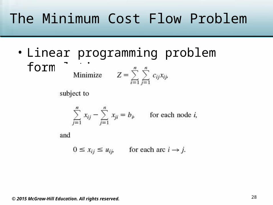
• General description of the minimum cost flow problem– The network is directed and connected– At least one of the nodes is a supply node,

and one of the other nodes is a demand node• All remaining nodes are transshipment nodes

– Flow is only allowed in direction of the arrowhead

• Arc capacity gives maximum allowable flow

25


The Minimum Cost Flow Problem

• General description (cont’d.)– Network has enough arcs with sufficient

capacity to enable all flow generated at supply nodes to reach all demand nodes

– Cost of flow through each arc is proportional to the amount of flow

– Objective: minimize total cost of sending available supply through the network to meet the given demand

26



27



• Linear programming problem formulation

28



• Feasible solutions property

• Integer solutions property– For minimum cost flow problems where every

bi and uij have integer values, all the basic variables in every basic feasible solution also have integer values

29



• Special cases that fit the minimum cost flow problem– The transportation problem– The assignment problem– The transshipment problem– The shortest-path problem– The maximum flow problem

30



• Network simplex method– An alternative method to solving the special

cases when the special-purpose algorithms are not available

31


10.7 The Network Simplex Method

• Streamlined version of the simplex method– Same basic steps

• Finding the entering basic variable• Determining the leaving basic variable• Solving for the new BF solution

• General concepts of the method are covered in the text

32


The Network Simplex Method

• Incorporate the upper bound technique:– To deal with the arc capacity constraints

• Network representation of BF solutions– Basic arcs: arcs corresponding to basic

variables• Key property: they never form undirected cycles

– Nonbasic arcs: arcs corresponding to nonbasic variables

33



• BF solutions can be obtained by solving spanning trees– For arcs not in the spanning tree, set the

corresponding variables (xij or yij) equal to zero

– For arcs in the spanning tree, solve for the corresponding variables (xij or yij) in the system of linear equations provided by the node constraints

34



• Feasible spanning tree– Spanning tree whose solution from the node

constraints also satisfies all the other constraints

• Fundamental theorem for the network simplex method– Basic solutions are spanning tree solutions

(and conversely)– BF solutions are solutions for feasible

spanning trees (and conversely)35


10.8 A Network Model for Optimizing a Project’s Time-Cost Trade-off

• Network based OR techniques developed in the 1950s– PERT (Program Evaluation Review

Technique)– CPM (Critical Path Method)– Both are used in project management

• Concepts have merged into PERT/CPM

• CPM method for time-cost tradeoff– Addresses a project with a specific deadline

36


A Network Model for Optimizing a Project’s Time-Cost Trade-off

• CPM method for time-cost trade-off (cont’d.)– Problem: find optimal plan for expediting

activities to minimize the total cost of completing the project within the deadline

• General approach– Use a network to display the various activities

• And the order in which they need to be performed

– Form optimization model• Solve using linear programming

37



• Prototype example– The Reliable Construction Co. won the

contract to construct a new plant within a time period of 40 weeks

– See Table 10.7

• Project network options– Activity-on-arc (AOA)

• Each activity is represented by an arc• Nodes separate activities from predecessors• Used by original versions of PERT and CPM

38


39



• Project network options (cont’d.)– Activity-on-node (AON)

• Each activity is represented by a node• Arcs show precedence relationships between

activities• Has several advantages over AOA• May become the standard format for project

networks

40



• Path– One of the routes following the arcs from start

to finish

• The critical path– Relevant: length of each path through the

network– Sum of estimated durations of activities on the

path

41



• Estimating the critical path (project duration) for the Reliable Construction Co. example– See Pages 415-417 in the text

• Crashing an activity– Taking special costly measures to reduce an

activity’s duration– Crashing the project involves crashing a

number of activities

42


43


• Example problem: determine least expensive way to crash activities to reduce overall duration to 40 weeks

• Solution methods– Marginal cost analysis

• See Table 10.10 and Table 10.11 on Pages 419 and 420 of the text

– Linear programming• Follow steps on Pages 420-424 of the text


10.9 Conclusions

• Problems addressed with network models– Optimizing an existing network– Designing a new network

• Minimum spanning tree problem

• CPM method of time-cost trade-offs– Powerful way of applying network optimization

to project management

44

Documents

Network Optimization Models - Welcome - The Citadel - …macs.citadel.edu/zhangli/Courses-Taught/F… · PPT file · Web view · 2014-09-11Network consists of a set of points and