Embed Size (px)
Citation preview
USDOT Region V Regional University Transportation Center Final Report
Report Submission Date: October 15, 2009
IL IN
WI
MN
MI
OH
NEXTRANS Project No 012IY01
Sensor Network Design for Multimodal Freight Transportation
Systems
By
Xiaopeng Li Ph.D. student
Civil and Environmental Engineering University of Illinois, Urbana-Champaign
and
Eunseok Choi Undergraduate student
Civil and Environmental Engineering University of Illinois, Urbana-Champaign
and
Yanfeng Ouyang Principal Investigator
Assistant Professor of Civil and Environmental Engineering University of Illinois, Urbana-Champaign

DISCLAIMER
Funding for this research was provided by the NEXTRANS Center, Purdue University under
Grant No. DTRT07-G-005 of the U.S. Department of Transportation, Research and Innovative
Technology Administration (RITA), University Transportation Centers Program. The contents of
this report reflect the views of the authors, who are responsible for the facts and the accuracy
of the information presented herein. This document is disseminated under the sponsorship of
the Department of Transportation, University Transportation Centers Program, in the interest
of information exchange. The U.S. Government assumes no liability for the contents or use
thereof.
USDOT Region V Regional University Transportation Center Final Report
TECHNICAL SUMMARY
NEXTRANS Project No 012IY01Technical Summary - Page 1
IL IN
WI
MN
MI
OH
NEXTRANS Project No 012IY01 Final Report, October 2009
Sensor Network Design for Multimodal Freight Transportation Systems
Introduction The agricultural and manufacturing industries in the US Midwest region rely heavily on the efficiency of
freight transportation systems. While the growth of freight movement far outpaces that of the
transportation infrastructure, ensuring the efficiency and sustainability of the transportation networks
becomes a major challenge. The prominent disbenefit of delay and unreliability highlights the need for
an integrated, systems-level framework that incorporates cutting-edge information technologies and
advanced multimodal network modeling techniques to monitor, manage and plan complex freight
transportation systems. Recent developments in sensing and information technology hold the promise
to allow efficient monitoring, assessment, and management of complex systems.
Findings This project investigated the effect of existing or off-the-shelf sensors on detecting traffic and infrastructure conditions for highway and rail modes. This research project developed an analytical framework to quantify the benefits and costs of deploying sensors for the major freight transportation modes. Specifically, this project developed a new sensor deployment problem in the context of traffic O-D flow surveillance using vehicle ID inspection technologies (e.g., RFID). In addition to traditional flow coverage benefits based on individual sensors, we investigated the path coverage benefits from synthesizing the multiple sensors in transportation networks. We considered possible sensor disruptions that are very common for many sensor technologies, yet not well addressed until very recently. A reliable location design model framework was proposed to optimize sensor deployment benefit. This model considered both flow and path coverage, while allowing for probabilistic sensor failures. A set of efficient algorithms were developed and tested on moderate-size problem instances. We found that the LR-based algorithm had the best performance for the tested problems. The greedy-algorithm can yield good solutions if flow coverage benefit is significant. Then we applied this model to the large-scale Chicago intermodal network, where the highway network, the railroad network and their connections were considered in this study. We extracted detailed input flow data from limited data resources. We examined the qualities of solutions of different algorithms, the best of which (from the LR-based algorithm) are analyzed to draw out managerial insights about sensor deployment. The experiments showed that path coverage benefit is more sensitive to sensor failures and installation budget. It was also found that path coverage tends to spread out sensor locations while high failure probabilities tend to cluster sensors together.

NEXTRANS Project No 012IY01Technical Summary - Page 2
Recommendations Future work can be conducted in several directions. First of all, the proposed model addresses probabilistic sensor failures but assumes known O-D flow paths. This may be reasonable in the freight operation context but a more comprehensive model that encompasses traffic routing and assignment will be desirable. In addition, the current model assumes all sensor failures are independent with equal probability. Yet more complex sensor failure patterns (e.g, site-dependent and correlated failures) are not uncommon in the real world. Additional work that relaxes these two assumptions is needed. Finally, it will be interesting to explore how alternative traffic surveillance benefits would affect the optimal sensor deployment pattern.
Contacts
For more information:
Yanfeng Ouyang Principal Investigator Civil and Environmental Engineering University of Illinois, Urbana-Champaign [email protected] (217) 333-9858 (217) 333-1924 Fax
NEXTRANS Center Purdue University - Discovery Park 2700 Kent B-100 West Lafayette, IN 47906 [email protected] (765) 496-9729 (765) 807-3123 Fax www.purdue.edu/dp/nextrans

USDOT Region V Regional University Transportation Center Final Report
Report Submission Date: October 15, 2009
IL IN
WI
MN
MI
OH
NEXTRANS Project No 012IY01
Sensor Network Design for Multimodal Freight Transportation
Systems
By
Xiaopeng Li Ph.D. student
Civil and Environmental Engineering University of Illinois, Urbana-Champaign
and
Eunseok Choi Undergraduate student
Civil and Environmental Engineering University of Illinois, Urbana-Champaign
and
Yanfeng Ouyang Principal Investigator
Assistant Professor of Civil and Environmental Engineering University of Illinois, Urbana-Champaign

i
ACKNOWLEDGMENTS
The data preparation tasks for the Chicago multimodal network case study was partly
supported through the participation of Eunseok Choi in the 2009 NEXTRANS
Undergraduate Summer Internship Program.

ii
TABLE OF CONTENTS
Page
LIST OF FIGURES ........................................................................................................... iii
CHAPTER 1. INTRODUCTION ....................................................................................... 1
1.1 Background and motivation .................................................................................1
1.2 Literature review and study objectives ................................................................2
1.3 Organization of the research ................................................................................5
CHAPTER 2. MODELING AND SOLUTION TECHNIQUES ....................................... 6
2.1 Model introduction ..............................................................................................6
2.2 Solution approach ..............................................................................................11
2.2.1 Greedy algorithm ...................................................................................... 12
2.2.2 LR-based Algorithm ................................................................................. 13
2.3 Algorithm test ....................................................................................................17
CHAPTER 3. CASE STUDY: THE INDOT-MAINTAINABLE NETWORK .............. 22
3.1 Data preparation .................................................................................................22
3.2 Results ................................................................................................................27
CHAPTER 4. CONCLUSIONS ....................................................................................... 33
4.1 Summary ............................................................................................................33
4.2 Future research directions ..................................................................................34
REFERENCES ................................................................................................................. 35
iii
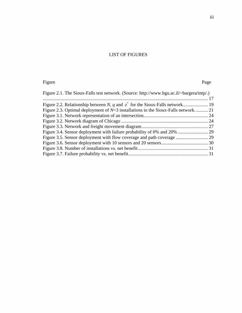
LIST OF FIGURES
Figure Page
Figure 2.1. The Sioux-Falls test network. (Source: http://www.bgu.ac.il/~bargera/tntp/.)........................................................................................................................................... 17 Figure 2.2. Relationship between N, q and for the Sioux-Falls network. .................... 19 *zFigure 2.3. Optimal deployment of N=3 installations in the Sioux-Falls network. .......... 21 Figure 3.1. Network representation of an intersection ...................................................... 24 Figure 3.2. Network diagram of Chicago ......................................................................... 24 Figure 3.3. Network and freight movement diagram ........................................................ 27 Figure 3.4. Sensor deployment with failure probability of 0% and 20% ......................... 29 Figure 3.5. Sensor deployment with flow coverage and path coverage ........................... 29 Figure 3.6. Sensor deployment with 10 sensors and 20 sensors ....................................... 30 Figure 3.8. Number of installations vs. net benefit ........................................................... 31 Figure 3.7. Failure probability vs. net benefit ................................................................... 31
1
CHAPTER 1. INTRODUCTION
1.1 Background and motivation
The US Midwest region generates about 20 percent of the nation's overall gross
domestic product (GDP). The backbone industries (such as agriculture and
manufacturing) and regional economy are heavily dependent of the efficiency of regional
freight transportation systems. While the transportation infrastructure development has
reached a plateau in recent years (approximately one percent increase of lane miles per
year) 1, the volume of freight movement has been growing, and will continue to grow,
dramatically. It is estimated that the number of freight trucks in the Midwest states will
increase by more than 60 percent by 2020 (Meiller 2007). As the demand for freight
transportation infrastructure continues to grow at an increasing pace, ensuring the
efficiency and sustainability of the transportation networks for current and future
generations is a major challenge. Nationwide, after 40 years of steady declination, freight
logistics costs have been rising again in both absolute quantity and percentage GDP. A
significant portion of this cost increase has been attributed to the deterioration of delay
and unreliability in our highly congested freight transportation systems across modes
(highway, rail, ocean waterway). This poses prominent disbenefits to the society and
highlights the need for an integrated, systems-level framework that incorporates cutting-
edge information technologies and advanced multimodal network modeling techniques to
monitor and manage the complex freight transportation systems. Such an integrated
framework will enable decision makers to (1) understand conditions of multiple system
components (traffic, infrastructure, etc.) at various spatial and temporal scales, and (2)
2
identify effective planning and management solutions to achieve desirable operating
conditions and ensure efficient operations of freight transportation across modes.
Recent developments in sensing and information technology and its applications to
the field of transportation hold the promise to allow efficient monitoring, assessment,
management, and planning of complex networks with system-wide interactions among
multiple system components. This is possible by combining information from parallel
sensing systems with integrated multi-scale modeling and decision support. State
transportation agencies have made significant investment in deploying various types of
sensors (e.g., loop detectors, RFID transponders) on state and local highways, which
enable a wide range of fundamental applications in traffic management systems (TMS)
such as traffic condition surveillance (e.g., incident detection), prediction (e.g., travel
time estimation), and control (e.g., freeway ramp metering and traffic diversion). Prior
success on traffic database development and travel time prediction have demonstrated the
benefit of collecting traffic and speed data from loop detectors, radar sensor stations, and
toll collection transponders. The railroads have also invested millions of dollars in
advanced sensing technology (e.g., track-side machine vision devices) to monitor railcar
traffic.
1.2 Literature review and study objectives
Sensor technologies (e.g., loop detectors, surveillance cameras, radio frequency
identifications/RFID) have been widely used on transportation networks. Real-time
traffic information is sampled by these sensors to monitor traffic status and to develop
control strategies. The effectiveness of a traffic surveillance system depends on not only
the accuracy of the sampled information but also the coverage over the transportation
network. However, implementing these new technologies usually requires large
investment. Accuracy and coverage are often two conflicting objectives due to limited
resources: collecting high-quality information usually relies on sophisticated and
expensive technologies and thus limited budget would restrict the number of installations;
on the other hand, due to the limited effective range of most sensors, complete coverage

3
over a network usually requires dense installations. To balance this trade-off, intensive
studies have been conducted to determine efficient and reliable deployment of
surveillance systems. Yang et al. (1991) conducted a robust analysis on the utility of
traffic counting points for traffic O-D flow estimation. Yang and Zhou (1998) proposed a
sensor deployment framework to maximize such utility. This framework has been
extended to accommodate turning traffic information (Bianco et al., 2001), existing
installations and O-D information content (Ehlert et al., 2006), screen line problem (Yang
et al., 2006), time-varying network flows (Fei et al., 2007; Fei and Mahmassani, 2008)
and railcar inspection under potential sensor failures (Ouyang et al., 2009).
Despite numerous studies on O-D flow coverage, research on the usage of sensors
for network O-D travel time estimation has been relatively scarce. To the best of our
knowledge, only Banet al. (2009) developed sensor deployment algorithm for travel time
estimation in a single freeway corridor---little research has addressed the problem in
general networks. Accurate travel time estimation provides important information for
decision support in both private sectors (e.g., tacking fleets for trucking companies,
traveler information provision) and public agencies (e.g., congestion mitigation, accident
management). For a transportation network, we may want to know as much as possible
the real-time travel time between all possible O-D pairs. However, traditional
surveillance technologies (e.g., loop detectors) would encounter significant challenges
due to their inability to accurately capture O-D flows (Kerner and Rehborn, 1996; Li et
al., 2009). New sensor technologies, on the other hand, are able to identify vehicle IDs
and therefore hold the promise to overcome these challenges by synthesizing vehicle ID
information from different sensors. For example, the consecutive time stamps of a vehicle
at two sensor locations would provide an accurate estimate of travel time.
Despite numerous studies on O-D flow coverage, research on the usage of sensors
for network O-D travel time estimation has been relatively scarce. To the best of our
knowledge, only Ban et al. (2009) developed sensor deployment algorithm for travel time
estimation in a single freeway corridor---little research has addressed the problem in
general networks. Accurate travel time estimation provides important information for
decision support in both private sectors (e.g., tacking fleets for trucking companies,
4
traveler information provision) and public agencies (e.g., congestion mitigation, accident
management). For a transportation network, we may want to know as much as possible
the real-time travel time between all possible O-D pairs. However, traditional
surveillance technologies (e.g., loop detectors) would encounter significant challenges
due to their inability to accurately capture O-D flows (Kerner and Rehborn, 1996; Li et
al., 2009). New sensor technologies, on the other hand, are able to identify vehicle IDs
and therefore hold the promise to overcome these challenges by synthesizing vehicle ID
information from different sensors. For example, the consecutive time stamps of a vehicle
at two sensor locations would provide an accurate estimate of travel time.
Like many other IT technologies, most existing sensors are subject to performance
disruptions due to system errors, adverse weather conditions, or intentional sabotages
(Rajagopal and Varaiya, 2007; Carbunar et al., 2005). Intuitively, such failures may
substantially impair the surveillance effectiveness. Potential disruptions need to be
addressed in a reliable design so that the sensor system not only has a good performance
in the normal scenario but also is resilient against possible loss in failure scenarios. In
recent years, reliable facility location problems have been studied in the supply chain
design (Daskin, 1983; Snyder and Daskin, 2005; Cui et al., 2009; Li and Ouyang, 2009)
and railroad defect detection sensor design contexts (Ouyang et al., 2009). However,
despite these recent efforts, few studies in the network traffic surveillance context have
addressed the possibility of sensor failures.
This research aims to fill these gaps. It builds on the reliable facility location
literature and develops a linear integer model to determine optimal locations for vehicle
ID inspection sensors for travel time estimation as well as traffic O-D flow count. The
model allows probabilistic sensor failures in general transportation networks. The
formulated problem is complex by nature, and the real-world instances are generally of
large scale. This imposes prohibitive computational burden if we solve this model with
standard solvers. We therefore propose customized algorithms to solve the problem
efficiently. Case studies are conducted to test the algorithms and to draw insights.

5
1.3 Organization of the research
The remainder of the research is organized as follows. Chapter 2 develops the
mathematical model and proposes different algorithms to solve this problem. The
performance of these algorithms is tested with a moderate-size example. We found the
Lagrangian-relaxation-based algorithm outperforms the others in general. Chapter 3
applies this model to a large-scale real problem, the Chicago intermodal network. A set of
data-processing procedures including heuristics have been taken to extract detailed input
from limited macroscopic data. Managerial insights are drawn from result analysis.
Chapter 5 summarizes the research and provides future research directions.
6
CHAPTER 2. MODELING AND SOLUTION TECHNIQUES
This chapter introduces the model formulation and solution algorithms. Section
2.1 formulates the problem into a mathematical model. Section 2.2 introduces solution
algorithms and analyzes their properties. Section 2.3 tests these algorithms with a
moderate-scale example and discusses their performances.
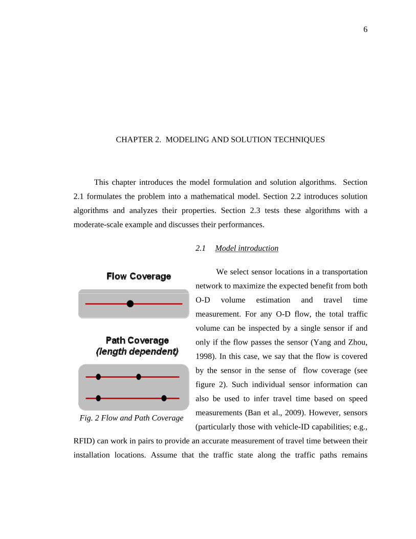
2.1 Model introduction
We select sensor locations in a transportation
network to maximize the expected benefit from both
O-D volume estimation and travel time
measurement. For any O-D flow, the total traffic
volume can be inspected by a single sensor if and
only if the flow passes the sensor (Yang and Zhou,
1998). In this case, we say that the flow is covered
by the sensor in the sense of flow coverage (see
figure 2). Such individual sensor information can
also be used to infer travel time based on speed
measurements (Ban et al., 2009). However, sensors
(particularly those with vehicle-ID capabilities; e.g.,
RFID) can work in pairs to provide an accurate measurement of travel time between their
installation locations. Assume that the traffic state along the traffic paths remains
Fig. 2 Flow and Path Coverage

7
relatively stable during the nominal travel time. 1 Intuitively, accurate travel time
estimation for an O-D path benefits all traffic on this path, while the accuracy depends on
the span of sensors---the wider a pair of sensors span over an O-D path, the larger portion
of the path is measured and the better it helps to estimate travel time of that O-D path.
Thus the travel time surveillance benefit, which we denote by path coverage (see figure
2), depends on not only the inspected traffic volume but also the lengths of covered O-D
paths by sensor pairs. We assume for simplicity that path coverage for an O-D path is
proportional to both its traffic volume and covered length.
Let be the set of O-D paths on the network. Each path i is specified by its
traffic volume
I ∈ I
if , which is assumed to be deterministic and known. Each path passes a
set of candidate locations, , where sensors can be potentially installed. Each candidate
location j on path i has a corresponding mileage, , increasing along the traffic
direction of
i
iJ
ijm
if . The collection of all candidate locations over the network is .
For convenience of notation, let
: ii∀
=∪J J
jI denote the set of paths that pass the same location j.
Note that ∪ . j =j∀
I I
Due to limited budget, no more than N sensors can be built on the network. For
ji∀ ∈I , if is inspected if an operational sensor is located at j. Similar to the traditional
maximal covering models (Yang and Zhou, 1998), if if is inspected by at least one sensor,
the benefit of flow coverage is , where is a nonnegative coefficient. If c ib f cb if passes at
least two sensors, we can record its travel time between the first functioning (head)
sensor it passes, at location hj , and the last functioning (rear) sensor it passes, at
location ej . The benefit of path coverage can be expressed as , where
is also a nonnegative coefficient.
( et i ij ijb f m m− )h tb
1 Without losing generality a path can be divided into multiple short segments to make this assumption reasonable.

8
In the long run, sensors may be disrupted or malfunctional from time to time.
When sensors fail, the flow coverage and path coverage patterns in the network also
change. Hence we consider the expected surveillance benefit across all sensor failure
scenarios in addition to the ideal non-failure scenario. The head (or rear) sensor for each i
may vary over different failure scenarios. In other words, different head (or rear) sensors
are assigned to i according to failure scenarios. Sensors on i can be ranked into different
priority levels according to such head (or rear) assignment such that in any scenario the
sensor with the lowest level among all functioning ones, if available, is the head (or rear)
sensor. In the normal scenario (without any failure), the most upstream sensor on i serves
as the head sensor, and thus it is the level-zero head sensor for i. If this sensor fails, its
immediately downstream sensor takes over to serve i, and thus this second sensor is the
level-one head sensor for i. This process can be repeated to label every installed sensor on
i with a unique head sensor assignment level. Similarly, each sensor on i can be labeled
with a unique rear sensor assignment level that starts from zero for the most downstream
sensor and increases upstream. Supposing that there are sensors installed on path i,
we see that once the locations with installations on i are given (i.e.,
iS
0 1 1{ , ,.., }i
i i iSj j j −
ordered from upstream to downstream), their head and rear assignment levels are
determined by the following simple rule
Definition 1. (valid assignment rule) A sensor at location isj is the level-s head sensor
and the level- ( rear sensor for traffic path i. 1 )iS − − s
Since each sensor installed on i receives a unique head (or rear) assignment level to
i, there are at most : min(| |, )i iR N= J
−
, levels of possible head (or rear) assignment. Let
denote a possible head (or rear) assignment level for a sensor on i. 0,1, , 1ir R=
The primal decision variables : { }jx=x determine where to install sensors, where
1, if a sensor is installed at location ;0, otherwise.j
jx
⎧= ⎨⎩

9
Given , the auxiliary variables x { }ijrh=h and { }ijrh=e decide how sensors are
assigned to paths according to the valid assignment rule; i.e.,
1, if a sensor is installed at and it is assigned to as a level- head sensor;0, otherwise,ijr
j i rh
⎧= ⎨⎩
and
1, if a sensor is installed at and it is assigned to as a level- rear sensor;0, otherwise.ijr
j i re
⎧= ⎨⎩
Assume that each sensor fails independently with an identical probability 0 1q≤ < .
The objective of this two-sensor-covering problem (TSC) is to maximize the expected
total benefit of flow coverage and path coverage for all O-D paths.
1
,0
(TSC) max ( ) : max (1 ) [ ( ) ],i
i
Rr
i j i t ij ijr t ij c ijrr
z q q f b m h b−
∈ ∈=
= − − +∑ ∑ ∑x h ex I J m b e+ (1)
subject to ,j jx N∈ ≤∑ J (2)
1
0, ,
iR
ijr j ir
h x i j−
=
= ∀ ∈ ∀ ∈∑ I J ,
,
(3)
1
0, ,
iR
ijr j ir
e x i j−
=
= ∀ ∈ ∀ ∈∑ I J (4)
1, , 0;ij ijrh i r∈ ≤ ∀ ∈ =∑ J I (5a)
( 1) , , 1, ,i ij ijr j ij r ih h i r R∈ ∈ − 1,≤ ∀ ∈ ∀ = −∑ ∑J J I (5b)
, , 0,1, ,i ij ijr j ijr ie h i r R∈ ∈ 1,≤ ∀ ∈ ∀ = −∑ ∑J J I (6)
, , {0,1}, , , 0,1, , 1j ijr ijr i ix h e i j r R .∈ ∀ ∈ ∀ ∈ ∀ = −I J (7)
Constraint (2) enforces the budget limit, while constraints (3) - (7) postulate the valid
assignment rule. Constraints (3) (or (4)) ensure that each installed sensor is assigned to
each of its corresponding paths at one and only one head (or rear) assignment level.
Constraints (5) and (6) indicate that no more than one head or rear sensor is assigned to

10
each path at each level, and each rear assignment must be accompanied by a head
assignment. Constraints (6) also imply that for each path i, all the implemented head
assignment levels, { | 1}ij ijrr h∈ =∑ J , start from 0 and form a consecutive sequence.
Constraints (7) postulate all decision variables to be binary.
The following proposition reveals the relationship between the above formulation
and the valid assignment rule.
Proposition 1: The optimal solution to the TSC problem (1)-(7) satisfies the valid
assignment.
Proof . Let , , denote the optimal solution to TSC. Again locations with installed
sensors on each path i are indexed with
*x *h *e
0 1 1{ , ,.., }i
i i iSj j j − from upstream to downstream.
Let denote the set of all implemented head assignment levels to i; i.e.,
. Similarly, let
hiR
: { | }hjrR 1ih
ii jr ∈= ∑ J = : { |i
ei jr ∈ 1}ijre= =∑ JR . For the case of 0q = ,
there is no failure and only the level-0 assignment affects the objective value. It is
obvious that the optimal solution enforces all non-trivial assignments (at level-0) to be
consistent with the valid assignment rule.
Now we consider the case with $q>0$. Since each installed sensor on
$i$ corresponds to only one implemented head (or rear) assignment level (from (3) and
(4)) and different sensor cannot have the same head (or rear) assignment level (from (5)
and (6)), it is obvious that | | | |h ei i Si= =R R .
For the head assignment, due to constraints (5), contains a sequence of levels
from 0 to . Due to constraints (6), . Thus
hiR
1iS − ei ⊆R Rh
i {0,1, , 1}h ei i iS= = −R R , and
we denote them by . Therefore on path i, each sensor iR sij is labeled with a unique head
(or rear) assignment level in . At optimality, a more upstream sensor shall have a
lower head assignment level and a higher rear assignment level. Thus
iR
isj corresponds to

11
the level-s head assignment and the level- ( 1 )iS s− − rear assignment to i, which is the
valid assignment rule.
It shall be noted that the TSC modal can be easily adapted for cases where existing
installations are already present (Ehlert et al., 2006). We simply enforce if a sensor
is already installed at location j; the model still has the same structure and complexity.
1jx =
2.2 Solution approach
We have built a linear integer mathematical program that determines sensor
deployment to optimize traffic surveillance benefits from both individual sensor flow
coverage (e.g., for traffic volume statistics) and synthesized sensors (e.g., for travel time
estimation). This model builds on the reliable facility location literature and allows
sensors to be subject to probabilistic failures (e.g., due to technical flaws or
environmental hazards). The formulated problem is complex by nature, which imposes a
prohibitive computational burden on solving this problem with commercial solvers (e.g.,
CPLEX). We therefore propose customized greedy and Lagrangian relaxation algorithms
to solve the problem efficiently. These proposed algorithms are applied to this project to
yield very good results, while CPLEX often has difficulty in solving most of tested
instances. Those who are interested in details are referred to Li and Ouyang (2009).
TSC is NP-hard because the maximal covering problem is a special case of TSC
(with and ). As we will show in Section 4, commercial optimization software
(e.g., CPLEX) would work well only for small-scale instances but it usually runs into
difficulty when problem size increases. We hence propose customized algorithms to
obtain near-optimal solutions for large-scale problems. The first algorithm is based on a
simple greedy heuristic, which can yield good solutions for many realistic applications.
But it does not provide information on how close these solutions are from the true optima.
Hence we propose a second algorithm based on Lagrangian relaxation (LR), which
provides not only good feasible solutions but also optimality gaps.
0tb = 0q =
12
2.2.1 Greedy algorithm
The greedy algorithm for TSC simply selects sensor locations sequentially based
on the best marginal increase of objective (1), until all N installation locations have been
selected. The exact steps are as follows.
Step 0: Initialization. Let the set of selected location indices and the iteration
index . Set ;
:=∅Q
: 1n = 0,jx j= ∀ ∈J
Step 1: Search for the location that will bring the maximum marginal improvement
of objective ; i.e., select
thnthn *
\arg max { ( ) : 1, iff { }}.k jj z x j k∈ ′ ′= = ∈x ∪J Q Q
: ( )n z z
The
corresponding marginal objective improvement is denoted by ( )ρ ′= −x x ,
where *1, { }j iff x j j′ ∪Q= ∈ . Let * 1j
x = and *{ }j= ∪Q Q .
Setp 2: If n=N, stop and return x and the corresponding objective value 1
N
nn
ρ=∑ ;
otherwise, , and go to step 1. 1n n= +
Greedy heuristic is widely applied to many practical problems not only because of
its simplicity but also due to its reasonable practical performance. For example, in case of
the classic maximal covering problem (a special case of TSC where q=0 and bt=0), Feige
(1998) proved that the objective value of any greedy solution is no smaller than
of the true optimum; i.e., the approximation ratio is (1 1/ )e− / ( 1)e e− . More importantly,
no known polynomial-time algorithm can beat the greedy algorithm in terms of this
approximation ratio bound (Feige, 1998). We can obtain a similar approximation ratio for
the maximal covering problem with probabilistic facility failures (a special case of TSC
where and ). 0=tb 0q >
For general TSC, however, the approximation ratio of the proposed greedy
algorithm is not bounded. This can be seen from the following simple example. Suppose
a network has three nodes {1,2,3}=J
0af
, two links {( , and two consecutive O-D
flow paths, i.e., with
1,2), (2,3)}
{ , }a b=I , 1bf= = , and {1,2}a =J and . If {2,3}b =J 0cb = ,

13
0tb > and , a possible solution from the greedy algorithm is , which
yields . Yet the optimal solution is obviously
2N =
) 0=
{1,2}=Q
(z x {2,3}=Q , which gives a positive
objective value. Hence, the proposed greedy algorithm for TSC does not have a
performance bound, and we propose an LR-based algorithm in the next section.
2.2.2 LR-based Algorithm
2.2.2.1 Relaxed subproblems and bounds
We relax constraints (5) and (6), and add them to the objective (1) with
nonnegative Lagrangian multipliers { }irλ λ= and { }irγ=γ , respectively. The relaxed
TSC (RTSC) becomes:
1
, ,0
( , ) : max ( )i
i
R
R i j ijrr
, 0minλ γ 0i ih E(RTSC) ijr ijr ijrz H eλ γ λ−
≥ ∈=
⎡∈ ∈
⎤= + +⎢ ⎥
⎦∑ I
⎣∑ ∑ ∑x h e I J (8)
s.t. (2)-(4) and (7),
where the benefit of an installation at location j as a level-r head sensor for any ji∈I is
( 1)(1 ) , 0 ;(1 ) ,
i t ij ir i r irr
i t ij ir ir
q q f b m rq q f b m
λ λ γλ γ
+− − − + + −− − − +
,1, , 21,i
i
Rr R
== −
r⎧⎪= ⎨⎪⎩
(1rE q
ijrH
ijr
(9)
and the benefit of this installation as a level-r rear sensor is
) ( )i t ij c irq f b m b γ+ − . (10) = −
For any given λ and γ , the exact value of Rz ( , )λ γ provides an upper bound of (1),
and it can be obtained from the following decomposition scheme. When (5) and (6) are
relaxed, assignments are no longer dependent across j. Constraints (3) require that the
hear assignment of each j with sensor installed is conducted at exactly one level for each
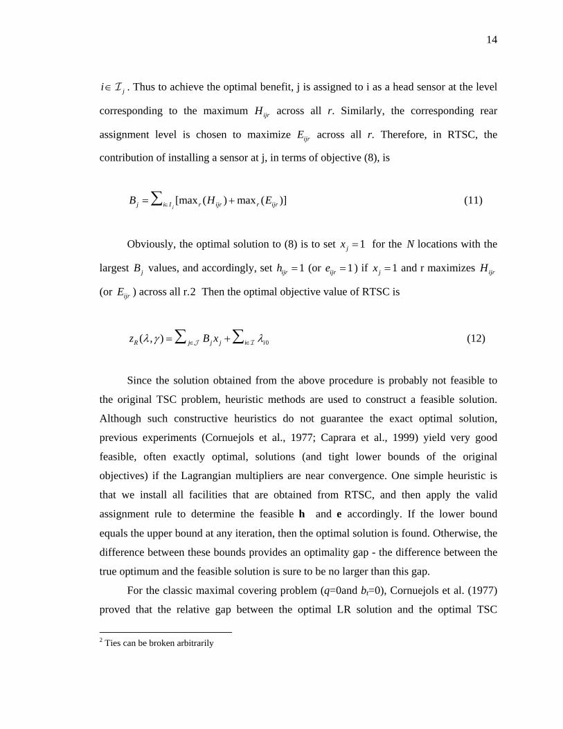
14
ji∈I . Thus to achieve the optimal benefit, j is assigned to i as a head sensor at the level
corresponding to the maximum across all r. Similarly, the corresponding rear
assignment level is chosen to maximize
ijrH
ijrE across all r. Therefore, in RTSC, the
contribution of installing a sensor at j, in terms of objective (8), is
[max ( ) ma )]jj i I r ijrB H∈= +∑ x (r ijrE (11)
Obviously, the optimal solution to (8) is to set 1jx = for the N locations with the
largest jB values, and accordingly, set ijrh 1= (or 1ijre = ) if 1jx = and r maximizes
(or
ijrH
ijrE ) across all r.2 Then the optimal objective value of RTSC is
0ix( , )R j j jz B iλ γ λ∈+∈=∑ ∑J I (12)
Since the solution obtained from the above procedure is probably not feasible to
the original TSC problem, heuristic methods are used to construct a feasible solution.
Although such constructive heuristics do not guarantee the exact optimal solution,
previous experiments (Cornuejols et al., 1977; Caprara et al., 1999) yield very good
feasible, often exactly optimal, solutions (and tight lower bounds of the original
objectives) if the Lagrangian multipliers are near convergence. One simple heuristic is
that we install all facilities that are obtained from RTSC, and then apply the valid
assignment rule to determine the feasible h and accordingly. If the lower bound
equals the upper bound at any iteration, then the optimal solution is found. Otherwise, the
difference between these bounds provides an optimality gap - the difference between the
true optimum and the feasible solution is sure to be no larger than this gap.
e
For the classic maximal covering problem (q=0and bt=0), Cornuejols et al. (1977)
proved that the relative gap between the optimal LR solution and the optimal TSC
2 Ties can be broken arbitrarily

15
solution is bounded by 1/e. This bound holds for more general problems with positive
failure probability q>0.
It should be noted that the computational time for solving the RTSC problem (8)
and for obtaining an feasible solution are bounded by and
, respectively.
( | | | | )i iO N R∈⋅ + ∑ II J
( | |O N ⋅ I )
2.2.2.2 Multiplier updating
Function ( , )Rz λ γ is known to be convex over λ and γ . RTSC can be solved with
an iterative subgradient search. We update λ and γ iteratively to find the tightest upper
bound ,minλ γ 0 ( , )Rz λ γ≥ add subscript k to distinguish variables in iteration k . The
initial values of the multipliers are obtained with heuristics (e.g., the dual solution to the
linear relaxation of the original problem). At the end of each iteration, multipliers are
updated as follows.
. We
−
−
)
( )1 max 0, , , 0,1, , 1,k k k kir ir ir it i r Rλ λ λ+ = + Δ ∀ ∈ ∀ =I
( )1 max 0, , , 0,1, , 1,k k k kir ir ir it i r Rγ γ γ+ = + Δ ∀ ∈ ∀ =I
where the subgradients are
, ( 1)
1, 0:
, otherwisei
i
kir j ijr
j ij r
rh
hλ ∈
∈ −
=⎧⎪Δ = − ⎨⎪⎩
∑ ∑JJ
and . Step size is usually set to : (i
kir j ijr ijre hγ ∈Δ = −∑ J kt
12 2
0
( ( , ) ) ,( ) ( )
i
k k k LBk R
Rk k
i ir irr
z zt μ λ γ
λ γ−
∈=
−=
⎡ ⎤Δ + Δ⎣ ⎦∑ ∑I

16
where kμ is a control scaler, and is the objective value of the best-known feasible
solution. Traditionally, control scaler
LBzkμ is determined by setting and halving 0 2μ =
kμ if (Rz , )k kλ γ
0μ
is not improved after a fixed number of iterations (Fisher, 1981). This
approach is modified by (Fisher, 1981) Caprara et al. (1999) for faster convergence. The
idea is to set , and compare the best and worst values of 0.1= ( ,kRz )kλ γ in every
certain number (e.g., 20) of iterations: decrease kμ if the difference is greater than a
larger threshold (e.g., 1% ) and increase kμ if the difference is less than a smaller
threshold (e.g., 0.1%). In our case study, we use the traditional approach when multipliers
are far from their optimal values and then switch to the second approach near
convergence.
In principle, the LR algorithm is terminated if one of the following conditions is
satisfied: (i) the lower bound equals the upper bound, (ii) the optimality gap stops
reducing, and (iii) the solution time exceeds a reasonable limit. Our experience shows
that condition (ii) terminates the algorithm most of the time. In case that happens, we
may use the following branch and bound procedure to further reduce the optimality gap.
2.2.2.3 Branch and bound
If the aforementioned LR algorithm ends up having a non-zero optimality gap, we
implement the LR algorithm into a branch and bound framework. We branch on variables
in a depth-first manner, and use a greedy heuristic to choose the next variable x jx for
branching: installation at j shall bring in the greatest increase of the objective value (1)
given the variables that have already been branched. We branch each variable first to 1
(enforcing installation) and then to 0 (forbidding installation). At each node, we run the
LR algorithm to determine the lower and upper bounds, while extra constraints for
already-branched variables are exerted. If the upper bound is lower than the best feasible
solution so far, the node no longer has potential and is trimmed. If the current node has
already had N enforced or | | N−J forbidden installations, only one non-trivial feasible

17
solution exists and is returned as both the lower and the upper bounds. At each branching,
the multipliers of a parent node are passed down to its child nodes as their initial
multipliers.
2.3 Algorithm test
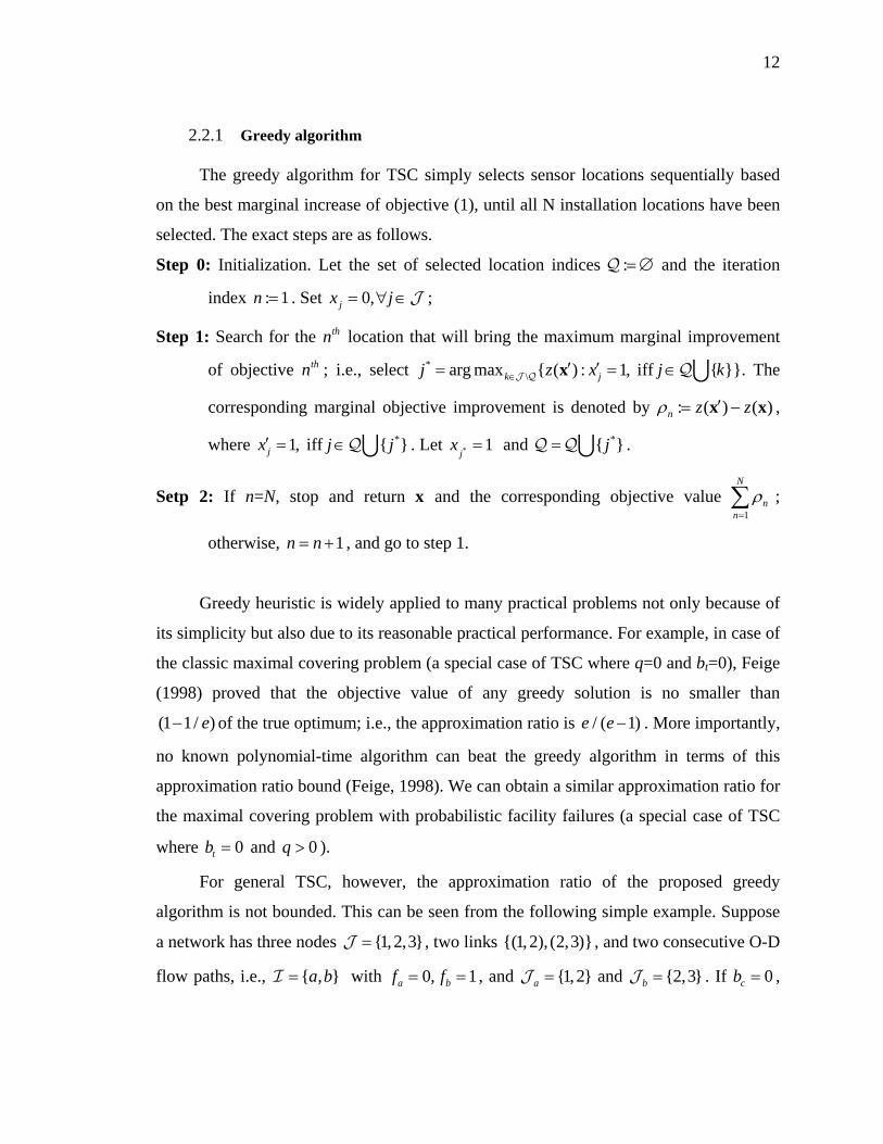
The Sioux-Falls network has 24 vertices and 76 links, as shown in Figure 2.1.
Assume that all the vertices are candidate locations, i.e., | = 24. There are 528 traffic
O-D pairs. For simplicity, we assume that each O-D pair only has one flow path that is
determined by the shortest path algorithm5, and hence | = 528. Assume too that the
sensor at a node can detect all traffic passing that node from different directions.
|J
|I
1
8
4 5 63
2
15 19
17
18
7
12 11 10 16
9
20
23 22
14
13 24 21
3
12
6
8
9
11
5
15
122313
21
16 19
17
2018 54
55
50
48
2951 49 52
58
24
27
32
33
36
7 35
4034
41
44
57
45
72
70
46 67
69 65
25
28 43
53
59 61
56 60
66 62
6863
7673
30
7142
647539
74
37 38
26
4 14
22 47
10 31
Figure 2.1. The Sioux-Falls test network. (Source: http://www.bgu.ac.il/~bargera/tntp/.)
18
The experiments are implemented on a PC with 2.0 GHz CPU and 2 GB memory.
We set a solution time limit of 1800 seconds, and run a series of instances 1tb = ,
, , and {0,1,10}cb ∈ {3,5,7}N ∈ {0,0.05,0.2,0.5}q∈ . The results are summarized in
Table 1. In this table, denote the optimal objective value for the LR-based algorithm by
, the solution time by T, and the optimality gap by ε . The objective value found by the
greedy algorithm by . For comparison, we solve the same instances with commercial
software CPLEX, and let , and be the objective value, the solution time and the
residual optimality gap, respectively. Let
*zGz
zC CT Cε
: / (t tb b )cbα = + be an indicator of the relative
importance of path coverage benefit.3 As we can see, the LR-based algorithm found
optimal solutions for almost all the instances ( 0%=ε ). CPLEX has a comparable
performance only when α is small (i.e., flow coverage dominates). Otherwise, the
performance of CPLEX is significantly worse than the LR-based algorithm: CPLEX
cannot find the optimal solution within 1800 seconds for many instances, and sometimes
it even cannot find a meaningful feasible solution (where 0Cz = or ). The
greedy algorithm finds a good feasible solution (i.e.,
INF%C =ε*Gz z≈ ) when α is small. For most
instances with 1α = , however, the results from the greedy algorithm are quite far from
the optima. This implies that the greedy algorithm does not work as well when path
coverage is the dominating objective. This is probably because a sensor's contribution to
path coverage highly depends on other sensors' locations.
3 Note that once α is fixed, scaling the value of (or ) does not affect the optimal sensor deployment. tb cb
19
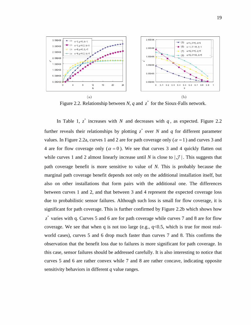
Figure 2.2. Relationship between N, q and for the Sioux-Falls network. *z
In Table 1, increases with and decreases with q , as expected. *z N Figure 2.2
further reveals their relationships by plotting over N and q for different parameter
values. In
*z
Figure 2.2a, curves 1 and 2 are for path coverage only ( 1α = ) and curves 3 and
4 are for flow coverage only ( 0α = ). We see that curves 3 and 4 quickly flatten out
while curves 1 and 2 almost linearly increase until N is close to | . This suggests that
path coverage benefit is more sensitive to value of N. This is probably because the
marginal path coverage benefit depends not only on the additional installation itself, but
also on other installations that form pairs with the additional one. The differences
between curves 1 and 2, and that between 3 and 4 represent the expected coverage loss
due to probabilistic sensor failures. Although such loss is small for flow coverage, it is
significant for path coverage. This is further confirmed by
|J
Figure 2.2b which shows how
varies with q. Curves 5 and 6 are for path coverage while curves 7 and 8 are for flow
coverage. We see that when q is not too large (e.g., q<0.5, which is true for most real-
world cases), curves 5 and 6 drop much faster than curves 7 and 8. This confirms the
observation that the benefit loss due to failures is more significant for path coverage. In
this case, sensor failures should be addressed carefully. It is also interesting to notice that
curves 5 and 6 are rather convex while 7 and 8 are rather concave, indicating opposite
sensitivity behaviors in different q value ranges.
*z
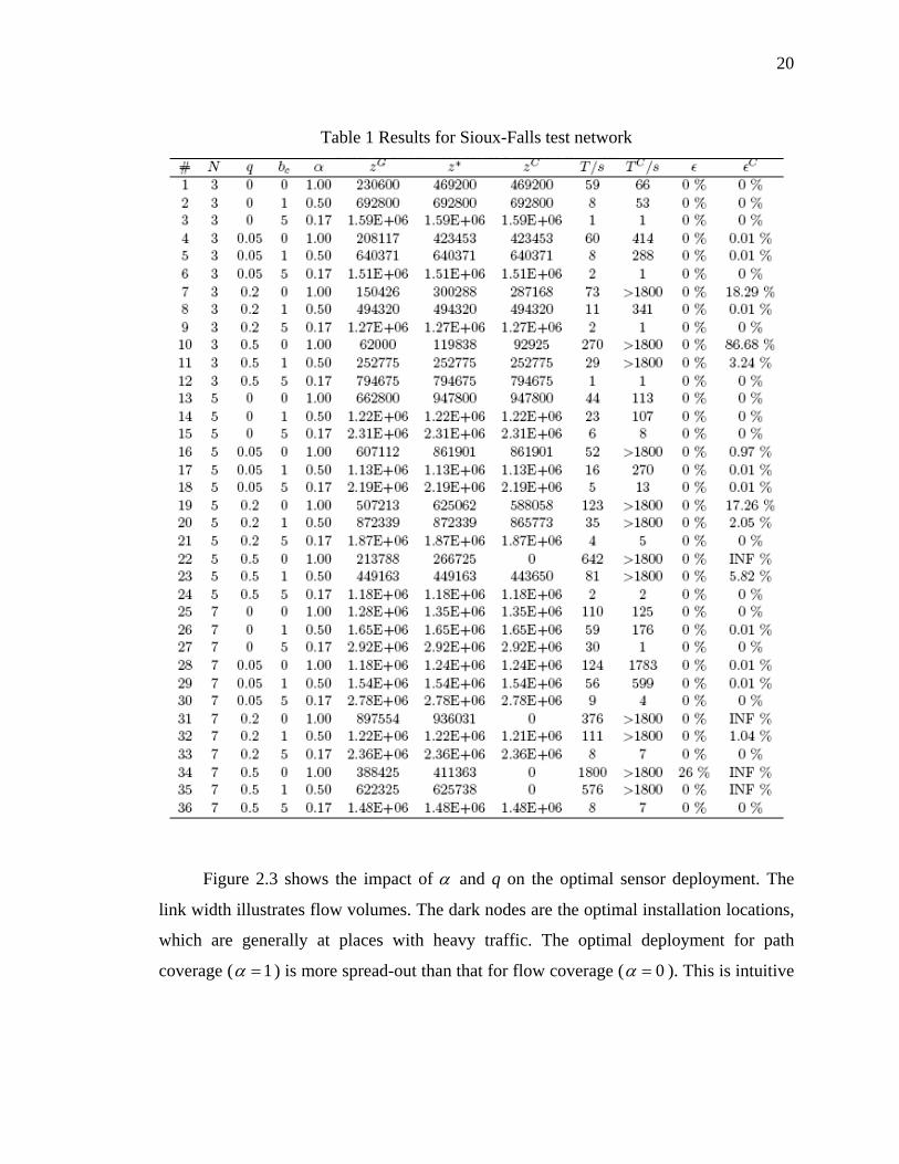
20
Table 1 Results for Sioux-Falls test network
Figure 2.3 shows the impact of α and q on the optimal sensor deployment. The
link width illustrates flow volumes. The dark nodes are the optimal installation locations,
which are generally at places with heavy traffic. The optimal deployment for path
coverage ( 1α = ) is more spread-out than that for flow coverage ( 0α = ). This is intuitive

21
because more scattered sensor pairs can cover longer paths. On the other hand, higher
failure probability generally leads to a higher degree of sensor clustering.
Figure 2.3. Optimal deployment of N=3 installations in the Sioux-Falls network.

22
CHAPTER 3. CASE STUDY: THE INDOT-MAINTAINABLE NETWORK
Chapter 3 discusses the application of the proposed model to a large-scale real
problem, the Chicago intermodal network. Section 3.1 introduces how to obtain input
data by integrating multiple data sources. Heuristics are taken to extract detailed
information from limited data with coarse granularity. Section 3.2 analyzes solutions with
different algorithms for a set of instances. Managerial insights are drawn on how
coverage measure and failure probabilities influence optimal sensor deployment.
3.1 Data preparation
Collecting accurate and quality data is very important to illustrate that the proposed
model and solution techniques can be applied to realistic scenarios. Without data or with
invalid data, the results of the experiments could be misleading. The data preparation
efforts consist of network portion and freight movement portion.
Network
We first had to figure out the network system in a simple and realistic way, and to
transform it in a mathematical representation. In Chicago, intermodal traffic is
transported through two networks: highway and rail. Unlike the highway network system
which is easily recognizable, rail network system is more complicated and harder to
access. Besides, there were simply not enough data available for rail traffic to figure out
complete picture of intermodal traffic movement. Our team decided to focus our network
on highway network and rail terminals where highway and rail interchange occurs. Here
are some of concepts and terms we defined regarding the network.

23
1. Access Point – An access point is an entrance point that connects the highway
network in Chicago and the outside world. There are 8 access points in the
Chicago network, and these points basically define the network boundary.
2. Conjunction – A conjunction is an interchange of two highways. Conjunctions
play an important role in this network as they represent the local population. To
represent Chicago population, we assumed that conjunctions are dominant over
local highway networks meaning conjunctions absorb all local population.
Basically, conjunctions function as local exits as we do not consider any local
exits.
o Sensors will be deployed at conjunctions: Logically, it makes sense to
install sensors at conjunctions rather than in the middle of highway since
traffic only can change their route at conjunctions.
3. Terminals – A terminal is basically a rail yard where freight transition occurs
between rail and truck. There are 17 terminals in Chicago land area, and their
locations are represented at the nearest highway exit for the purpose of not
dealing with local road networks.
4. Network Representation (Sheffi, 1985) – Recalling the limited effectiveness range
of RFID sensors (~31ft), one installation of RFID detection structure can only
cover one travel bound on a highway. In other words, to cover the entire
conjunction with RFID, all four directions of the conjunction needs to be installed
with RFID detection separately. To break down a conjunction, we used the
network representation approach developed by Yosef Sheffi in Urban
Transportation Networks in 1985. Figure 3.1 explains how a conjunction breaks
down into multiple nodes and directions.
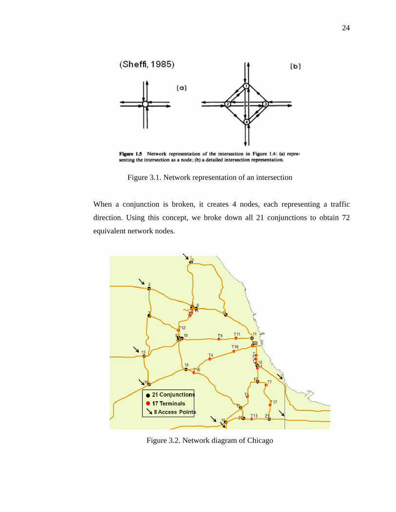
24
Figure 3.1. Network representation of an intersection
When a conjunction is broken, it creates 4 nodes, each representing a traffic
direction. Using this concept, we broke down all 21 conjunctions to obtain 72
equivalent network nodes.
Figure 3.2. Network diagram of Chicago

25
Figure 3.2 is the network diagram of Chicago highway and terminals. It shows all
the locations of conjunctions, terminals, and access points. After the coding of the
network, we obtained 89 total nodes, 353 total links, and 1046 O-D flows.
Freight Movement
Understanding the movement of intermodal freight traffic is a crucial part of the
data preparation efforts. The primary data source we used was from the website of
Bureau of Transportation Statistics.4 Given data that describes only a small portion of
the entire traffic, we had to utilize the data as much as possible to draw the most realistic
picture as possible. The data summary is shown in Table 2.
Table 2. Chicago freight volume table from Bureau of Transportation Statistics
(unit: thousand tons) Inbound Outbound
All Modes 384,554 398,993
Single Mode 371,023 381,750
Truck 312,279 294,611
Truck: Outer States 117,289 87,778
Rail 34,343 43,957
Multi Modes 5,926 9,864
1. Single Mode – Single mode traffic describes the freight traffic that is transported
by truck only and has Chicago as destination or origin. Inbound single mode 4 Commodity Flow Survey: Metropolitan Areas (2002) Retrieved June 20, 2009 from Bureau of Transportation Statistics Website: http://www.bts.gov/publications/commodity_flow_survey/2002/metropolitan_areas/chicago_naperville_michigan_city_il_in_wi_csa_il_part/index.html

26
traffic originates from other states and crosses an access point to enter the
network and ends up at local Chicago exits represented by conjunctions.
Outbound traffic starts at conjunctions and ends up in outer states. These traffic
volumes are obtained at the website of Bureau of Transportation Statistics under
Commodity Flow Survey 2002. The route that single mode traffic chooses is
based on the shortest path between Chicago and the metropolitan city of the state
of origin, and we assign that traffic volume to the access point they cross. After
assigning all the volume to the access points, then we use the gravity model
method to distribute the volume to 21 conjunctions according to nearby
population weights.
2. Intermodal – Intermodal traffic here describes freight traffic that travels on both
rail and highway. Inbound traffic travels by rail and gets dropped off at terminals
within the network. Then they travel from terminals to conjunctions by truck, and
that is the only part we are concerned about.
3. There are several assumptions we made to simplify the difficulty associated with
data scarcity. First, we ignored the traffic that goes through Chicago. Given
limited data, it was almost impossible to distinguish through traffic from others.
Moreover, as we suspected that most of through traffic would take more of
peripheral routes around metropolitan area rather than going through them, we
decided to take them out of the picture. Another area of uncertainty was the rail
terminal transaction freight volumes. Rail freight tonnage numbers are given, but
there is simply no data available for us to track down how the freight is
distributed or which route they take. Thus, we assumed that all rail freight volume
that is transported to the terminal is destined to conjunctions and vice versa.

27
Figure 3.3. Network and freight movement diagram
Figure 3.3 illustrates the Chicago network and the all the freight movements
around the network.
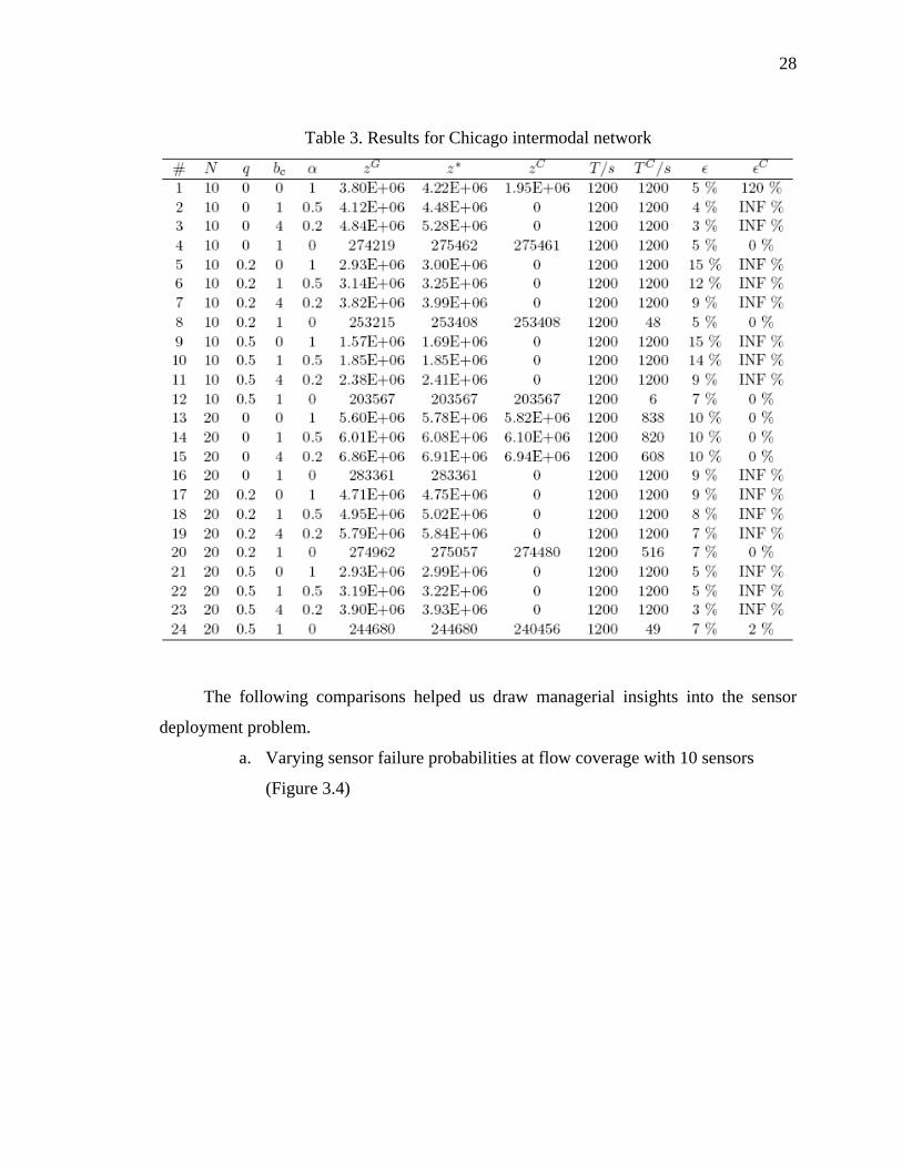
3.2 Results
We conducted a set of experiments on a PC with 2.0 GHz CPU and 2 GB memory
for the greedy algorithm, the LR-based algorithm, and CPLEX. The solution time limit is
set to be 1200 seconds. We have run a series of instances for , ,
, and . The results are summarized in
{0,1}tb ∈ {0,1,4}cb ∈
{10,20,30}N ∈ {0,0.2,0.5}q∈
15%≤
Table 3. Due to the
increased problem size, CPLEX cannot even get a meaningful feasible solution for most
instances. The LR-based algorithm always yields a near-optimum solution with a
reasonable residual gap ( ). From our experiments, the difference between the near-
optimal solution and the optimum is often much smaller than the residual gap. Thus these
solutions are suitable for engineering practice.
28
Table 3. Results for Chicago intermodal network
The following comparisons helped us draw managerial insights into the sensor
deployment problem.
a. Varying sensor failure probabilities at flow coverage with 10 sensors
(Figure 3.4)
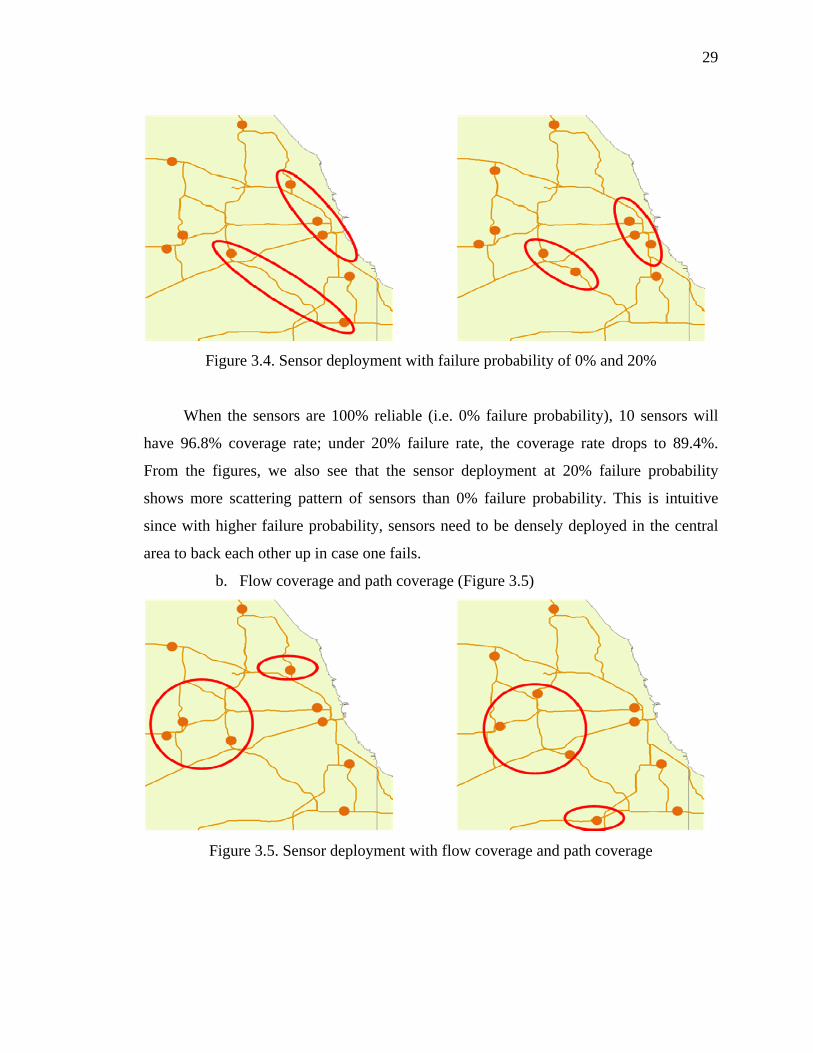
29
Figure 3.4. Sensor deployment with failure probability of 0% and 20%
When the sensors are 100% reliable (i.e. 0% failure probability), 10 sensors will
have 96.8% coverage rate; under 20% failure rate, the coverage rate drops to 89.4%.
From the figures, we also see that the sensor deployment at 20% failure probability
shows more scattering pattern of sensors than 0% failure probability. This is intuitive
since with higher failure probability, sensors need to be densely deployed in the central
area to back each other up in case one fails.
b. Flow coverage and path coverage (Figure 3.5)
Figure 3.5. Sensor deployment with flow coverage and path coverage
30
Then we compared flow and path coverage at 0% failure probability. Path coverage
showed a coverage rate of 67.8% which is a lot less than flow coverage. If we compare
the two big red circles in the diagram above, we see sensors in the path coverage scenario
are more spread apart than ones in flow coverage. Because the nature of path coverage is
to cover as much traffic as possible, path coverage scenario tends to prioritize quantity of
information over the quality of information.
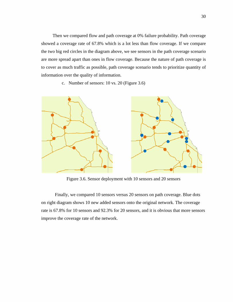
c. Number of sensors: 10 vs. 20 (Figure 3.6)
Figure 3.6. Sensor deployment with 10 sensors and 20 sensors
Finally, we compared 10 sensors versus 20 sensors on path coverage. Blue dots
on right diagram shows 10 new added sensors onto the original network. The coverage
rate is 67.8% for 10 sensors and 92.3% for 20 sensors, and it is obvious that more sensors
improve the coverage rate of the network.

31
Figure 3.7. Failure probability vs. net benefit
Figure 3.8. Number of installations vs. net benefit
Figures 3.7, 3.8 summarize the comparison of flow and path coverage. We
graphed the relationships between net benefit and failure probability and one between net
benefit and number of sensor installations. The general observation is that net benefit
increases at lower sensor probability and higher number of installations. The notable
insight we gain from these graphs is that path coverage benefit is much more sensitive

32
toward any changes in the network. From the graphs, we find that path coverage lines are
steeper than flow coverage lines, and that shows the sensitive nature of path coverage.
33
CHAPTER 4. CONCLUSIONS
This chapter summarizes the research, highlights its contributions, and proposes
directions for future research.
4.1 Summary
This research addresses a new sensor deployment problem in the context of traffic
O-D flow surveillance using vehicle ID inspection technologies (e.g., RFID). In addition
to traditional flow coverage benefits based on individual sensors, we investigated the path
coverage benefits from synthesizing the multiple sensors in transportation networks. We
consider possible sensor disruptions, that are very common for many sensor technologies,
yet not well addressed until very recently.
A reliable location design model framework is proposed to optimize sensor
deployment benefit. This model considers both flow and path coverage, while allowing
for probabilistic sensor failures. A set of efficient algorithms are developed, and tested on
a moderate-size problem. We find that the LR-based algorithm has good performance for
the tested problems. The greedy-algorithm can yield good solutions if flow coverage
benefit is significant.
Then we applies this model to the large-scale Chicago intermodal network. We
study both highway and railroad networks and their connections. We describe our efforts
to extract detailed input flow data from limited data resources. We examine the qualities
of solutions of different algorithms, the best of which (from the LR-based algorithm) are
analyzed to draw out managerial insights about sensor deployment. The experiments
show that path coverage benefit is more sensitive to sensor failures and installation

34
budget. It is also found that path coverage tends to spread out sensor locations while high
failure probabilities tend to cluster sensors together.
4.2 Future research directions
Future work can be conducted in several directions. First of all, the proposed
model addresses probabilistic sensor failures but assumes known O-D flow paths. This
may be reasonable in the freight operation context but a more comprehensive model that
encompasses traffic routing and assignment will be desirable. In addition, the current
model assumes all sensor failures are independent with equal probability. Yet more
complex sensor failure patterns (e.g, site-dependent and correlated failures) are not
uncommon in the real world. Additional work that relaxes these two assumptions is
needed. Finally, it will be interesting to explore how alternative traffic surveillance
benefits would affect the optimal sensor deployment pattern.
35
REFERENCES
Renee Meiller, (2007). Midwest transportation coalition addresses regional freight
challenges. UW-Madison News. http://www.news.wisc.edu/13852.
Ban, X. J., Herring, R., Margulici, J., Bayen, A. M., 2009. Optimal sensor placement for
freeway travel time estimation. Presented at Transportation Research Board 88th Annual
Meeting, Jan 2009.
Bianco, L., Confessore, G., Reverberi, P., 2001. A network based model for traffic sensor
location with implications on O/D matrix estimates. Transportation Science 35 (1), 50-60.
Caprara, A., Fischetti, M., Toth, P., 1999. A heuristic method for the set covering
problem. Operations Research 47 (5), 730-743.
Carbunar, B., Ramanathan, M., Koyuturk, M., Grama, A., Ho®mann, C., 2005.
Redundant-reader elimination in RFID systems. In: Proceedings of the 2nd IEEE
International Conference on Sensor and Ad Hoc Communications and Networks
(SECON). Santa Clara, September 2005.
Cornuejols, G., Fisher, M. L., Nemhauser, G. L., 1977. Location of bank accounts to
optimize float: An analytic study of exact and approximate algorithms. Management
Science 23 (8), 789-810.
Cui, T., Ouyang, Y., Shen, Z. M., 2009. Reliable facility location under the risk of
disruptions. Operations Research (in press).
36
Daskin, M. S., 1983. A maximum expected covering location model: Formulation,
properties and heuristic solution. Transportation Science 17 (1), 48-70.
Ehlert, A., Bell, M. G., Grosso, S., 2006. The optimisation of traffic count locations in
road net-works. Transportation Research Part B 40 (6), 460 - 479.
Fei, X., Mahmassani, H. S., 2008. Two-stage stochastic model for sensor location
problem in a large-scale network. Presented at Transportation Research Board 87th
Annual Meeting, Jan 2008.
Fei, X., Mahmassani, H. S., Eisenman, S. M., 2007. Sensor coverage and location for
real-time traffic prediction in large-scale networks. Transportation Research Record 2039
(1), 1-15.
Feige, U., 1998. A threshold of ln n for approximating set cover. Journal of the ACM 45
(4), 314-318.
Fisher, M. L., 1981. The lagrangian relaxation method for solving integer programming
problems. Management Science 27 (1), 1-18.
Kerner, B., Rehborn, H., 1996. Experimental properties of complexity in tra±c °ow.
Physical Review Letters 53 (5), R4275-R4278.
Li, X., Ouyang, Y., 2009. A continuum approximation approach to reliable facility
location design under correlated probabilistic disruptions. Transportation Research Part B
(in press).
Li, X., Peng, F., Ouyang, Y., 2009. Measurement and estimation of traffic oscillation
properties. Transportation Research Part B (in press).
Ouyang, Y., Li, X., Barkan, C. P. L., Kawprasert, A., Lai, Y.-C., 2009. Optimal locations
of railroad wayside defect detection installations. Computer-Aided Civil and
Infrastructure Engineering, 24 (5), 309{319(11).
37
Rajagopal, R., Varaiya, P., 2007. Health of californias loop detector system. California
PATH Research Report,UCB-ITS-PRR-2007-13.
Sheffi, Y., 1985. Urban Transportation Networks: Equilibrium Analysis with
Mathematical Programming Methods. Prentice-Hall, Inc., Englewood Cliffs, N.J.
Snyder, L. V., Daskin, M. S., 2005. Reliability models for facility location: The expected
failure cost case. Transportation Sciense 39 (3), 400-416.
Yang, H., Iida, Y., Sasaki, T., 1991. An analysis of the reliability of an origin-destination
trip matrix estimated from traffic counts. Transportation Research Part B 25 (5), 351-363.
Yang, H., Yang, C., Gan, L., 2006. Models and algorithms for the screen line-based
traffic-counting location problems. Computers & Operations Research 33 (3), 836-858.
Yang, H., Zhou, J., 1998. Optimal traffic counting locations for origin-destination matrix
estimation. Transportation Research Part B 32 (2), 109-126.